PARTITIONED COUPLING VS. MONOLITHIC BLOCK-PRECONDITIONING APPROACHES FOR SOLVING STOKES-DARCY SYSTEMS

Abstract

We consider the time-dependent Stokes-Darcy problem as a model case for the challenges involved in solving coupled systems. Keeping the model, its discretization, and the underlying numerics for the subproblems in the free-flow domain and the porous medium constant, we focus on different solver approaches for the coupled problem. We compare a partitioned coupling approach using the coupling library preCICE with a monolithic block-preconditioned one that is tailored to different formulations of the problem. Both approaches enable the reuse of already available iterative solvers and preconditioners, in our case, from the $\text{{DuMu}}^{\text{{x}}}$ framework. Our results indicate that the approaches can yield performance and scalability improvements compared to using direct solvers: Partitioned coupling is able to solve large problems faster if iterative solvers with suitable preconditioners are applied for the subproblems. The monolithic approach shows even stronger requirements on preconditioning, as standard simple solvers fail to converge. Our monolithic block preconditioning yields the fastest runtimes for large systems, but they vary strongly with the preconditioner configuration. Interestingly, using a specialized Uzawa preconditioner for the Stokes subsystem leads to overall increased runtimes compared to block preconditioners utilizing a more general algebraic multigrid. This highlights that optimizing for the non-coupled cases does not always pay off.

Jenny Schmalfuss, Cedric Riethmüller, Mirco Altenbernd, Kilian Weishaupt and Dominik Göddeke

1 INTRODUCTION

Coupled systems of free flow adjacent to permeable media have a decisive role in many applications. Examples include the environmental sciences (soil water evaporation), medical contexts (intervascular exchange), material design (optimization of fuel cell water management) or technical applications (drying of perishable goods) to name just a few. Capturing the complex interplay between the two flow domains is essential, however, the governing systems of equations form a coupled problem which can become quite complex to solve. This even holds for single-phase-flow systems, such as a river flowing over its porous bed. In this paper, we deliberately restrict ourselves to a simple, stationary, single-phase-flow problem, i.e., creeping Stokes flow in the free-flow domain, while using Darcy’s law for the porous domain. While limiting the physical complexity of our model, we focus on the numerical solution of the arising coupled system using either fully monolithic coupled schemes or a partitioned, iterative approach.

We build our contribution on the following observation: Practitioners, in particular in the modeling community, often rely on sparse direct solvers for the (linearized) subproblems, e.g., Umfpack, Pardiso and SuperLU, see [4] for an overview. This holds when Matlab’s Backslash operator or its equivalent in SciPy are used, as they translate to one of these sparse direct solvers under the hood. Often this also applies to users of PDE software frameworks like $\text{{DuMu}}^{\text{{x}}}$ [11, 15], whose design is in fact aiming to minimize the users’ burden of having to deal with every single aspect of the simulation pipeline.

Two issues in this context are often overlooked: First, sparse direct methods for the linear(ized) system(s) do not scale well in terms of compute time and memory. Second, the ill-conditioning of a fully assembled monolithic system can lead to severe trustworthiness issues in the solution. Both issues typically only appear after a model and its corresponding simulation pipeline have been set up, i.e., when test problems are exchanged for real-world scenarios. Table 1 exemplarily shows the fill-in factors in Umfpack, when solving the monolithic variant of one of our model problems with the finite volume scheme described in Section 2. While the matrix density increases mostly linearly due to surface-to-volume arguments, the fill-in for the computed sparse LU decomposition is clearly nonlinear in terms of memory. Thus it translates to compute time for generating the decomposition, and subsequently to solving the linear system using the decomposition.

Table 1: Memory requirements for storing the sparse matrix and its decomposition measured as matrix entries per degree of freedom.

DoF	156	1 056	10 100	102 720	1 001 000
Discretization	$6\times 6$	$16\times 16$	$50\times 50$	$160\times 160$	$500\times 500$
System matrix	6.7	7.3	7.6	7.7	7.7
Umfpack	19.9	38.6	78.6	145.7	241.4

In this paper, we demonstrate how carefully devised iterative and thus scalable solvers can alleviate these issues for two different solution strategies for coupled problems: We consider both a partitioned coupling approach where the subproblems are solved alternately, and a monolithic approach that honors the saddle point structure of the system. The former is realized with the coupling library preCICE [5], while the latter is tailored to standard PDE frameworks like $\text{{DuMu}}^{\text{{x}}}$. An important part of our contribution is a thorough comparison of these fundamentally different approaches.

2 MODEL PROBLEM

We consider an instationary, coupled Stokes-Darcy two-domain problem. It comprises a free flow of an incompressible fluid over a porous medium, see Figure 1(a).

(a) Coupled problem illustration.

(b) Boundary conditions.

Figure 1: The instationary Stokes-Darcy problem and its boundary conditions.

We mark quantities that are associated with the free-flow domain with ^ff, and use ^pm to denote the porous medium. The domains are denoted by $\Omega^{\mathrm{ff}}$ and $\Omega^{\mathrm{pm}}$, and share the common boundary $\Gamma$. Boundaries that are not shared are called $\Gamma^{\mathrm{ff}}$ and $\Gamma^{\mathrm{pm}}$. The normal vectors $n^{\mathrm{ff}}$ and $n^{\mathrm{pm}}$ are orthogonal to $\Gamma$ and point outwards their respective domains. The time dependent quantities pressure $p$ and velocity $v$ are used to describe the flow in each domain. We use the transient and incompressible Stokes equations to model the free flow:

$$\frac{\partial v}{\partial t}+\nabla\cdot(-\nu\left(\nabla v^{\mathrm{ff}}+\nabla v^{\mathrm{ff,T}}\right)+\rho^{-1}p^{\mathrm{ff}}I) =0 \text{in }\Omega^{\mathrm{ff}}$$ (1)

$$\nabla\cdot v^{\mathrm{ff}} =0 \text{in }\Omega^{\mathrm{ff}}$$ (2)

Above, $\rho$ and $\nu$ are the fluid density and kinematic viscosity, and $I$ is a suitable identity map. In the porous medium, Darcy’s law and the continuity equation are used:

$$v^{\mathrm{pm}} =-K\mu^{-1}\nabla p^{\mathrm{pm}} \text{in }\Omega^{\mathrm{pm}}$$ (3)

$$\nabla\cdot v^{\mathrm{pm}} =0 \text{in }\Omega^{\mathrm{pm}}$$ (4)

$K$ is the intrinsic permeability of the porous medium and $\mu=\nu\rho$ the dynamic viscosity of the fluid. As coupling conditions [16], we use the continuity of the normal stresses (5), the Beavers-Joseph-Saffman condition [20] in equation (6) and the continuity of the normal mass fluxes (7):

$$n\cdot[(pI-\tau)n]^{\mathrm{ff}} =[p]^{\mathrm{pm}} \text{on }\Gamma$$ (5)

$$[(v+\sqrt{K}(\alpha_{\mathrm{BJ}}\mu)^{-1}\tau n)\cdot t_{\mathrm{ff,pm}}]^{\mathrm{ff}} =0 \text{on }\Gamma$$ (6)

$$[v\cdot n]^{\mathrm{pm}} =-[v\cdot n]^{\mathrm{ff}} \text{on }\Gamma$$ (7)

We use $n$ for the normal of the respective flow component, $\tau$ for the viscous stresses and $\alpha_{\mathrm{BJ}}$ is the Beavers-Joseph coefficient. Further, $t_{\mathrm{ff,pm}}$ is the basis of the tangent plane that describes the interface between $\Omega^{\mathrm{ff}}$ and $\Omega^{\mathrm{pm}}$. To close this system, boundary conditions for the nonshared domain boundaries are illustrated in Figure 1(b). Note that the pressure $p_{\text{in}}$ on the left free-flow boundary changes over time.

The system of equations is discretized with a first-order backward Euler scheme in time, and finite volumes in space [15]. In the Darcy domain, a two-point flux approximation is used for the finite volume approximation of the pressure [12, Chap. 4]. In the Stokes domain, a staggered grid is used for the quantities pressure and velocity, and the fluxes are approximated with an upwind scheme [15, 21]. In summary, the discrete model, to be solved for every time step, has the form

$$Ax=b\quad =\quad\begin{pmatrix}A^{\prime}&B^{\prime}\\ C^{\prime}&D^{\prime}\end{pmatrix}\begin{pmatrix}x^{\mathrm{ff}}\\ p^{\mathrm{pm}}\end{pmatrix}=\begin{pmatrix}b^{\mathrm{ff}}\\ 0\end{pmatrix}$$ (8)

$$=\quad\begin{pmatrix}\begin{bmatrix}V&B\\ C&0\end{bmatrix}&\begin{bmatrix}B^{\prime}_{1}\\ 0\end{bmatrix}\\ \begin{bmatrix}C^{\prime}_{1}&0\end{bmatrix}&D^{\prime}\end{pmatrix}\begin{pmatrix}\begin{bmatrix}v^{\mathrm{ff}}\\ p^{\mathrm{ff}}\end{bmatrix}\\ p^{\mathrm{pm}}\end{pmatrix}=\begin{pmatrix}\begin{bmatrix}g\\ 0\end{bmatrix}\\ 0\end{pmatrix}.$$ (9)

Formulation (8) is denoted as two-domain (td) formulation of the problem, because the matrix blocks correspond to the free-flow and porous-medium phase of the problem. Further, we dub equation (9) the pressure-velocity (pv) formulation, due to the correspondence of the matrix blocks to the variables pressure and velocity.

3 PARTITIONED COUPLING APPROACH

Partitioned coupling approaches are a common strategy to solve coupled problems. In our setting, this means that the flow fields in the two flow domains are calculated separately, and the coupling between the subdomains is ensured by exchanging information over the sharp interface $\Gamma$. The benefit of this approach is that existing, optimized solvers for the subdomains can be used. We rely on $\text{{DuMu}}^{\text{{x}}}$ for the subdomain solvers, and preCICE for the coupling.

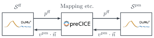
Figure 2: Subdomain coupling scheme implemented with preCICE.

Looking at the two-domain formulation (8), it is clear that boundary conditions on the common interface $\Gamma$ need to be exchanged in order to get a well-defined solution. For this, we use a serial implicit coupling technique [8] where the subdomain problems are solved sequentially and the boundary values for the other domain are written after the solution step is performed. The coupling procedure is depicted in Figure 2 and comprises a Dirichlet-Neumann coupling between the subdomains. We start the coupling by solving the free-flow problem, to determine Dirichlet pressure values on the interface $\Gamma$. The porous-medium-flow solver then determines Neumann velocity values on the interface. Thus, the pressure in the Darcy domain is fixed at the coupling interface $\Gamma$, and the Dirichlet-Neumann coupling leads to a well-defined solution. In more detail, let $k$ be the coupling iteration index and $v_{k}^{\mathrm{pm},\Gamma}$ the normal velocity at the interface $\Gamma$. The free-flow solver $\mathcal{S}^{\mathrm{ff}}$ computes a new flow state, which leads to an updated pressure $p_{k+1}^{\mathrm{ff},\Gamma}$ on the interface. With this updated pressure, the porous-medium-flow solver $\mathcal{S}^{\mathrm{pm}}$ computes a new flow state, which then leads to an updated normal velocity $v_{k+1}^{\mathrm{pm},\Gamma}$ on the interface. When we combine the two interface equations

$$\begin{drcases}\mathcal{S}^{\mathrm{ff}}\left(v_{k}^{\mathrm{pm},\Gamma}\right)&=p_{k+1}^{\mathrm{ff},\Gamma}\\ \mathcal{S}^{\mathrm{pm}}\left(p_{k+1}^{\mathrm{ff},\Gamma}\right)&=v_{k+1}^{\mathrm{pm},\Gamma}\end{drcases}\quad\Leftrightarrow\quad\mathcal{S}^{\mathrm{pm}}\left(\mathcal{S}^{\mathrm{ff}}\left(v_{k}^{\mathrm{pm},\Gamma}\right)\right)=v_{k+1}^{\mathrm{pm},\Gamma},$$ (10)

we can interpret the coupling scheme as an iterative solver for the fixed-point problem

$$\mathcal{S}^{\mathrm{pm}}\left(\mathcal{S}^{\mathrm{ff}}\left(v^{\mathrm{pm},\Gamma}\right)\right)=v^{\mathrm{pm},\Gamma}\quad\Leftrightarrow\quad R\left(v^{\mathrm{pm},\Gamma}\right):=\mathcal{S}^{\mathrm{pm}}\left(\mathcal{S}^{\mathrm{ff}}\left(v^{\mathrm{pm},\Gamma}\right)\right)-v^{\mathrm{pm},\Gamma}=0.$$ (11)

The scheme stops when the interface values converge, i.e., the fixed-point problem is solved to a prescribed accuracy. We emphasize that when the residual $R$ is sufficiently close to zero, we recover the monolithic solution.

Solving the fixed-point problem (11) with a Picard fixed-point iteration is prone to divergence for problems with strong instabilities or oscillations. In order to improve stability and convergence speed, fixed-point acceleration methods enrich the Picard iteration. These methods are applied as a post-processing step that we denote as $\mathcal{I}^{\mathrm{post}}$. Figure 3 illustrates our accelerated fixed-point iteration. Now, the flow update from the porous-medium solver is denoted by $\tilde{v}_{k+1}^{\mathrm{pm},\Gamma}$ (previously: $v_{k+1}^{\mathrm{pm},\Gamma}$), as it is the solution before the improvement by $\mathcal{I}^{\mathrm{post}}$.

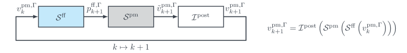
Figure 3: preCICE coupling scheme with enabled post-processing.

The post-processing scheme receives $\tilde{v}_{k+1}^{\mathrm{pm},\Gamma}$ from the porous-medium solver and computes an improved velocity $v_{k+1}^{\mathrm{pm},\Gamma}$. This new velocity depends on the current value and a history of previously calculated values. For our experiments, we choose the inverse least-squares interface quasi-Newton method [9] for the post-processing. This method approximates the inverse Jacobian of the residual operator $R$ of the nonlinear coupling equation, based on input-output relations. Then, it performs Newton-like update steps where a norm minimization is carried out. For more details on post-processing schemes and their implementation, see [8] and [5] respectively. To determine when the iteration can be stopped, we use the relative convergence measures

$$\left\lVert p_{k+1}^{\mathrm{ff},\Gamma}-p_{k}^{\mathrm{ff},\Gamma}\right\rVert_{2}<\varepsilon\left\lVert p_{k+1}^{\mathrm{ff},\Gamma}\right\rVert_{2}\qquad\text{and}\qquad\left\lVert\tilde{v}_{k+1}^{\mathrm{pm},\Gamma}-v_{k}^{\mathrm{pm},\Gamma}\right\rVert_{2}<\varepsilon\left\lVert\tilde{v}_{k+1}^{\mathrm{pm},\Gamma}\right\rVert_{2}.$$ (12)

Our choice of post-processing method and convergence measure is based on [14]. There, it is shown that for a similar model problem, the coupling approach as outlined above is consistent and converges to the monolithic solution. This finding is the basis for our convergence study in Section 5. As solvers $\mathcal{S}^{\mathrm{ff}}$ and $\mathcal{S}^{\mathrm{pm}}$, we use problem specific preconditioned iterative subdomain solvers in order to benefit from their smaller memory footprint, which results in a better numerical scaling with respect to the problem size.

preCICE follows a pure library approach, and is called from within $\text{{DuMu}}^{\text{{x}}}$  by the participating solvers, and not by the general framework. Through the library approach, the coupling is minimally invasive and provides a black-box functionality that allows us to use optimized solvers for the two domains.

4 MONOLITHIC BLOCK PRECONDITIONING

As an alternative to the partitioned approach, we consider a block-preconditioning strategy to iteratively solve the linear system in its entirety, allowing to consider both formulations (8) and (9) separately. The saddle point structure of $A^{\prime}$ implies one of the diagonal matrix blocks to be zero, which prevents the direct application of many preconditioning techniques like simple splitting based schemes [19, Chap. 10.2] or incomplete LU (ILU) preconditioning [17, 13]. To address this, we apply two types of block-preconditioning schemes that use exchangeable preconditioners for the respective matrix blocks. This allows to select the preconditioners for the matrix blocks based on structural or model-based properties of the block. The two considered block-preconditioning approaches are a block-Jacobi $\mathcal{P}_{\mathrm{BJ}}$ and a block-Gauss-Seidel preconditioning scheme $\mathcal{P}_{\mathrm{BGS}}$, which themselves are formulated to regard the linear system either as the $2\times 2$ block matrix (8) or as the $3\times 3$ block matrix (9).

To construct the $\mathcal{P}_{\mathrm{BJ}}$ preconditioners, we consider the block diagonal of the matrices (8) and (9). Additionally incorporating all block lower triangular parts is the basis for the $\mathcal{P}_{\mathrm{BGS}}$ preconditioners. Block-‘inverting’ those reduced block matrices yields the block preconditioners. The procedure to acquire the $\mathcal{P}_{\mathrm{BGS}}$ preconditioner is similar in spirit to [6]. There are two points to note: Firstly, an exact block inversion requires the exact inverses of the diagonal blocks, which is infeasible for preconditioners. We thus replace the inverses of the blocks $A^{\prime}$, $D^{\prime}$ and $V$ with preconditioners for these blocks that approximate the action of the exact inverses on the quantities of interest. We denote these block specific preconditioners by $\mathcal{P}_{A^{\prime}}$, $\mathcal{P}_{D^{\prime}}$ and $\mathcal{P}_{V}$. Secondly, we formally replace the zero block on the diagonal of the reduced matrix (9) with an identity matrix, preventing the ‘inversion’ of the zero block. In our implementation, this means that no preconditioner is applied to this block. We thus obtain general $\mathcal{P}_{\mathrm{BJ}}$ and $\mathcal{P}_{\mathrm{BGS}}$ preconditioner formulations.

In the implementation, a variety of concrete preconditioners for the respective matrix blocks can be used. For the two-domain formulation (8), this yields the two-domain block-Jacobi preconditioner $\mathcal{P}^{\mathrm{td}}_{\mathrm{BJ}}(\mathcal{P}_{A^{\prime}},\mathcal{P}_{D^{\prime}})$ and the two-domain block-Gauss-Seidel preconditioner $\mathcal{P}^{\mathrm{td}}_{\mathrm{BGS}}(\mathcal{P}_{A^{\prime}},\mathcal{P}_{D^{\prime}})$. Both depend on suitable preconditioners $\mathcal{P}_{A^{\prime}}$ and $\mathcal{P}_{D^{\prime}}$ for the blocks $A^{\prime}$ and $D^{\prime}$:

$$\mathcal{P}^{\mathrm{td}}_{\mathrm{BJ}}(\mathcal{P}_{A^{\prime}},\mathcal{P}_{D^{\prime}}) \coloneqq\begin{pmatrix}\mathcal{P}_{A^{\prime}}&0\\ 0&\mathcal{P}_{D^{\prime}}\end{pmatrix}, \mathcal{P}^{\mathrm{td}}_{\mathrm{BGS}}(\mathcal{P}_{A^{\prime}},\mathcal{P}_{D^{\prime}}) \coloneqq\begin{pmatrix}\mathcal{P}_{A^{\prime}}&0\\ -\mathcal{P}_{D^{\prime}}C^{\prime}\mathcal{P}_{A^{\prime}}&\mathcal{P}_{D^{\prime}}\end{pmatrix}$$ (13)

Likewise, we obtain the pressure-velocity block-Jacobi preconditioner $\mathcal{P}^{\mathrm{pv}}_{\mathrm{BJ}}(\mathcal{P}_{V},\mathcal{P}_{D^{\prime}})$ and the pressure-velocity block-Gauss-Seidel preconditioner $\mathcal{P}^{\mathrm{pv}}_{\mathrm{BGS}}(\mathcal{P}_{V},\mathcal{P}_{D^{\prime}})$. They depend on preconditioners $\mathcal{P}_{V}$ and $\mathcal{P}_{D^{\prime}}$ for the blocks $V$ and $D^{\prime}$:

$$\mathcal{P}^{\mathrm{pv}}_{\mathrm{BJ}}(\mathcal{P}_{V},\mathcal{P}_{D^{\prime}}) \coloneqq\begin{pmatrix}\mathcal{P}_{V}&0&0\\ 0&\text{I}&0\\ 0&0&\mathcal{P}_{D^{\prime}}\end{pmatrix}, \mathcal{P}^{\mathrm{pv}}_{\mathrm{BGS}}(\mathcal{P}_{V},\mathcal{P}_{D^{\prime}}) \coloneqq\begin{pmatrix}\mathcal{P}_{V}&0&0\\ -\text{I}C\mathcal{P}_{V}&\text{I}&0\\ -\mathcal{P}_{D^{\prime}}C^{\prime}_{1}\mathcal{P}_{V}&0&\mathcal{P}_{D^{\prime}}\end{pmatrix}$$ (14)

The differences between the four variants directly influence the possible choices of the sub-preconditioners $\mathcal{P}_{A^{\prime}}$, $\mathcal{P}_{D^{\prime}}$ and $\mathcal{P}_{V}$, as well as the computational efficiency of the whole block preconditioner. We begin with the difference between the two-domain $\mathcal{P}^{\mathrm{td}}_{*}$ and pressure-velocity $\mathcal{P}^{\mathrm{pv}}_{*}$ preconditioner formulations. The two-domain block preconditioners treat the saddle point structure of $A^{\prime}$ as one block. This permits specialized saddle point preconditioning techniques $\mathcal{P}_{A^{\prime}}$, like an Uzawa preconditioner [10], which may lead to better results due to their construction for the specific structure. The pressure-velocity formulation explicitly treats the saddle point structure by introducing an identity preconditioner on the critical diagonal block. This allows using a wider range of preconditioning techniques for $\mathcal{P}_{V}$ and $\mathcal{P}_{D^{\prime}}$, like splitting techniques, ILU(p) or algebraic multigrid (AMG) [3, 1] preconditioners. Also, this weakens the prerequisites on the preconditioners and allows using techniques that are not specialized for the problem’s structure.

Comparing the $\mathcal{P}_{\mathrm{BJ}}^{*}$ and $\mathcal{P}_{\mathrm{BGS}}^{*}$ preconditioners, the sparsity pattern of the block-Jacobi matrices suggests that their application requires fewer computational steps. The Gauss-Seidel preconditioners use additional coupling entries below the diagonal. Intuitively, one may expect an improved conditioning with a formulation that makes use of such additional information. However, this comes at the cost of more computation in the preconditioner application and setup. Without numerical experiments it is unclear whether the envisioned improvement of the system’s condition leads to shorter solution times compared to a preconditioner that is cheaper in its application but less capable to improve the systems condition number.

We highlight that preconditioners are commonly implemented as their application to vectors, i.e., for a vector $x$, it is of the form $\mathcal{P}(x)$. If such an implementation is already given, applying the block preconditioners to a blocked vector is a simple block matrix-vector product. This allows using existing preconditioner implementations within the blocked preconditioner. We use the ones available in $\text{{DuMu}}^{\text{{x}}}$ for our experiments.

5 COMPARISON AND RESULTS

We now assess the iterative solution of a coupled Stokes-Darcy system with partitioned coupling and block preconditioning, compared to the direct solver Umfpack [7]. We compare the runtime for solving increasingly large systems, and also comment on the memory requirement for all approaches. In the model problem from Section 2, we set $K=10^{-6}\text{m}^{2}$ and $\alpha_{\text{BJ}}=1.0$. The simulation is stopped at $t_{\text{end}}=50\cdot 10^{5}$s, with a time step size of $\text{d}t=2\cdot 10^{5}$s. A time dependent pressure difference is applied between the left and right boundary, which changes in the form of a half cosine-wave, with a maximum difference of $10^{-9}$Pa. The Stokes domain is a $1\times 3$ rectangle over a $1\times 1$ square for the Darcy domain, see also Figure 1. Each $1\times 1$ square uses the same number of spatial cells.

As solvers, we either use Umfpack, or preconditioned versions of the iterative solvers PD-GMRES [18] or Bi-CGSTAB [22]. As preconditioners we use an AMG method [3, 1], Uzawa-iterations [10] or an ILU(0) factorization [13, 17]. PD-GMRES uses $m_{\text{init}}=m_{\text{min}}=3$ and $m_{\text{step}}=5$, other parameters are chosen according to the original publication. Dune-Istl’s non-smooth aggregation AMG is used as solver or preconditioner, and performs one V-cycle [2, 3]. Pre- and post-smoothing is a single Gauss-Seidel iteration each with $\omega=1$. In our setup, we restrict ourselves to Umfpack  as coarse grid solver, and limit the hierarchy to 3 levels, which results in comparatively large coarse grid problems for the velocity blocks at scale. Our standard Uzawa configuration is an inexact Uzawa that executes one Richardson iteration where the optimal relaxation parameter $\omega_{\text{opt}}$ is estimated via power iteration. In the inexact case, the AMG method as specified above is used as solver, while Umfpack is used for the exact Uzawa iteration ($\text{Uzawa}_{e}$). All simulations are run on a single core of an AMD EPYC 7551P CPU with 2.0 GHz.

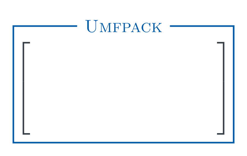
(a) Umfpack

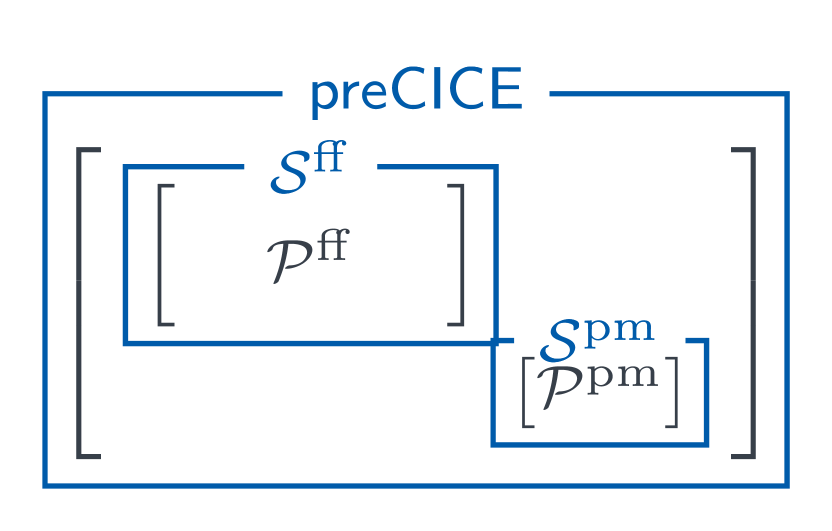
(b) preCICE

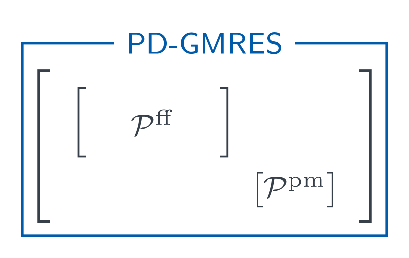
(c) Preconditioner $\mathcal{P}^{\mathrm{td}}$

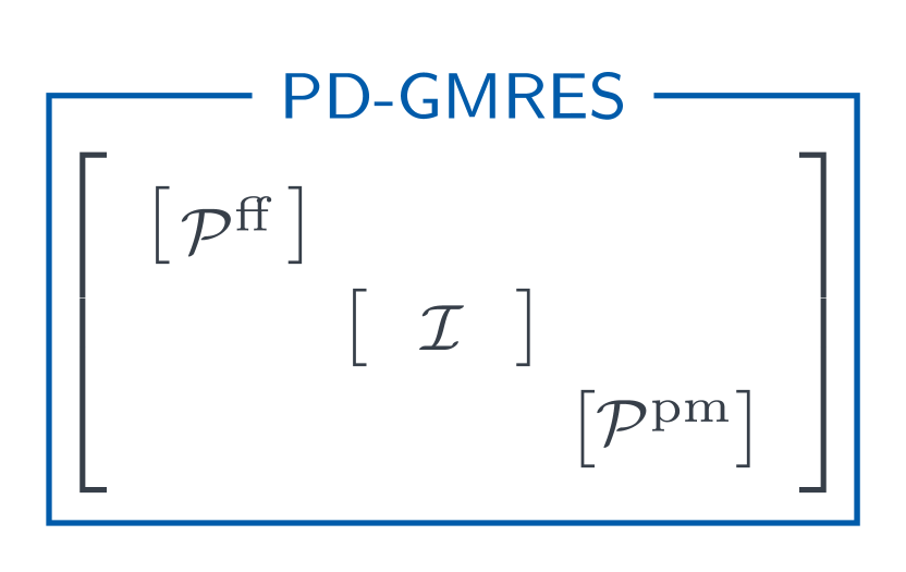
(d) Preconditioner $\mathcal{P}^{\mathrm{pv}}$

Figure 4: Evaluation setup conceptual visualization. Solvers are marked in blue around the matrix block they are applied to, preconditioners $\mathcal{P}$ are marked within their block.

Table 2: Evaluation setup comparison. Cells marked with n.a. are not applicable.

Name	Iterative	Monolithic	Solver			Preconditioner
			System	Stokes	Darcy	System	Stokes	Darcy
Umfpack	✗	✓	Umfpack	n.a.	n.a.	n.a.	n.a.	n.a.
preCICE Umfpack	✓	✗	preCICE	Umfpack	Umfpack	n.a.	n.a.	n.a.
preCICE $\mathcal{P}(\text{Uzawa}_{e},\text{AMG})$	✓	✗	preCICE	PD-GMRES	Bi-CGSTAB	n.a.	Uzawa-exact	AMG
preCICE $\mathcal{P}(\text{Uzawa},\text{AMG})$	✓	✗	preCICE	PD-GMRES	Bi-CGSTAB	n.a.	Uzawa	AMG
PD-GMRES $\mathcal{P}^{\mathrm{pv}}_{\mathrm{BJ}}(\text{AMG},\text{AMG})$	✓	✓	PD-GMRES	n.a.	n.a.	B-Jacobi	AMG	AMG
PD-GMRES $\mathcal{P}^{\mathrm{pv}}_{\mathrm{BGS}}(\text{AMG},\text{AMG})$	✓	✓	PD-GMRES	n.a.	n.a.	B-Gauss-Seidel	AMG	AMG
PD-GMRES $\mathcal{P}^{\mathrm{td}}_{\mathrm{BJ}}(\text{Uzawa},\text{AMG})$	✓	✓	PD-GMRES	n.a.	n.a.	B-Jacobi	Uzawa	AMG
PD-GMRES $\mathcal{P}^{\mathrm{td}}_{\mathrm{BGS}}(\text{Uzawa},\text{AMG})$	✓	✓	PD-GMRES	n.a.	n.a.	B-Gauss-Seidel	Uzawa	AMG
PD-GMRES $\mathcal{P}^{\mathrm{td}}_{\mathrm{BJ}}(\text{Uzawa},\text{ILU(0)})$	✓	✓	PD-GMRES	n.a.	n.a.	B-Jacobi	Uzawa	ILU(0)
PD-GMRES $\mathcal{P}^{\mathrm{td}}_{\mathrm{BGS}}(\text{Uzawa},\text{ILU(0)})$	✓	✓	PD-GMRES	n.a.	n.a.	B-Gauss-Seidel	Uzawa	ILU(0)

Figure 5: Runtime comparison of the direct solver Umfpack and iterative solvers with partitioned coupling and block preconditioning.

Figure 6: Runtime comparison of the best performing solver configurations.

To assess the runtime scaling of our different approaches, we increase the number of degrees of freedom. As baseline, we solve the linear system (9) with the direct solver Umfpack. The evaluations tested for the two iterative schemes are listed in Table 2, and schematically illustrated in Figure 4. The iterative methods are stopped when the residual’s norm is in the same order of magnitude as the Umfpack’s residual.

Figure 5 shows the measured runtime scaling behavior. To allow a comparison between the approaches, we choose the preconditioners for the subsystems to be either AMG or Uzawa. We observe that using iterative methods pays off in terms of runtime already for moderate problem sizes with $10^{4}$ degrees of freedom, benefiting from their better numerical scaling with respect to the problem size $n$. Partitioned coupling with preconditioned iterative solvers is able to outperform Umfpack for large $n$, while using the partitioned coupling approach with Umfpack for both subsystems is not beneficial and always slower than directly applying Umfpack to the monolithic system. The performance of our block-preconditioning approach yields the fastest runtimes for large systems, but varies strongly with the preconditioner configuration. Interestingly, we observe that using the specialized Uzawa preconditioner for Stokes in $\mathcal{P}^{\mathrm{td}}_{*}$ leads to increased runtimes compared to the less specialized $\mathcal{P}^{\mathrm{pv}}_{*}$ block preconditioner with two AMG preconditioners. In general, the $\mathcal{P}_{\mathrm{BJ}}^{*}$ configurations lead to slightly improved runtimes compared to the corresponding $\mathcal{P}_{\mathrm{BGS}}^{*}$ preconditioners.

In Figure 6 we show that tweaking the preconditioner configurations has the potential to further speed up the runtime, especially for the block-preconditioning approaches. While Umfpack scales roughly as $O(n\cdot\log(n))$, our partitioned and block-preconditioned approaches suggest a linear runtime increase with respect to the problem size $n$. In general, this behavior is also expected for the $\mathcal{P}^{\mathrm{pv}}_{*}(\text{AMG},\text{AMG})$ approaches but due to our setup we see an increase in runtime to a level similar to the Umfpack setting. This is caused by our restriction to use Umfpack as coarse grid solver in the preconditioner, and limiting the multigrid hierarchy to 3 levels: The resulting comparatively large coarse grid problems for the velocity blocks start to dominate the overall runtime. Increasing the multigrid hierarchy and/or switching to more efficient iterative solver for the coarse grid problems is expected to reduce the runtimes to or below the level of our $\mathcal{P}^{\mathrm{td}}_{*}(\text{Uzawa},\text{ILU(0)})$ approaches.

In terms of memory requirements both considered approaches are very similar when configured to use the same iterative solver(s) and preconditioners. Then, the memory consumption is dominated by the auxiliary vectors used by the iterative solvers to solve the linear system - in parts or as a whole. If limited memory is an issue, the partitioned coupling approach has the advantage to solve one subsystem at a time, requiring only the memory for solving the current subsystem.

6 CONCLUSION AND FUTURE WORK

Our experiments clearly indicate that both partitioned coupling and block-preconditioning approaches yield superior performance compared to using a sparse direct solver. This holds already for moderate problems sizes in single-threaded computations, and we expect the benefits to be substantially larger in parallel computations. Our implementation in $\text{{DuMu}}^{\text{{x}}}$ is very general, and can in principle also be applied for the nonlinear Navier-Stokes case, or for coupled flows involving more physics. Initial experiments show that our sophisticated coupling/preconditioning techniques are then obligatory, as simple monolithic iterative schemes fail due to the severe ill-conditioning.

7 ACKNOWLEDGEMENTS

This work was financially supported by the German Research Foundation (DFG), within the Collaborative Research Center on Interface-‐Driven Multi-‐Field Processes in Porous Media (SFB 1313, Project Number 327154368).

References

- [1] Peter Bastian, Markus Blatt and Robert Scheichl “Algebraic multigrid for discontinuous Galerkin discretizations of heterogeneous elliptic problems” In Numerical Linear Algebra with Applications 19.2 Wiley Online Library, 2012, pp. 367–388
- [2] Markus Blatt and Peter Bastian “The Iterative Solver Template Library” In International Workshop on Applied Parallel Computing, 2006, pp. 666–675 Springer
- [3] Markus Blatt, Olaf Ippisch and Peter Bastian “A Massively Parallel Algebraic Multigrid Preconditioner Based on Aggregation for Elliptic Problems with Heterogeneous Coefficients”, 2012
- [4] Matthias Bollhöfer, Olaf Schenk, Radim Janalík, Steve Hamm and Kiran Gullapalli “State-of-the-Art Sparse Direct Solvers”, https://arxiv.org/abs/1907.05309, 2019
- [5] Hans-Joachim Bungartz, Florian Lindner, Bernhard Gatzhammer, Miriam Mehl, Klaudius Scheufele, Alexander Shukaev and Benjamin Uekermann “preCICE – A fully parallel library for multi-physics surface coupling” Advances in Fluid-Structure Interaction In Computers and Fluids 141 Elsevier, 2016, pp. 250–258 DOI: https://doi.org/10.1016/j.compfluid.2016.04.003
- [6] Mingchao Cai, Mo Mu and Jinchao Xu “Preconditioning Techniques for a Mixed Stokes/Darcy Model in Porous Media Applications” In Journal of Computational and Applied Mathematics 233.2, 2009, pp. 346–355 DOI: 10.1016/j.cam.2009.07.029
- [7] Timothy A. Davis “UMFPACK User Guide” In Website: http://www.suitesparse.com, 2018
- [8] Joris Degroote “Partitioned Simulation of Fluid-Structure Interaction” In Archives of Computational Methods in Engineering 20, 2013, pp. 185–238 DOI: 10.1007/s11831-013-9085-5
- [9] Joris Degroote, Klaus-Jürgen Bathe and Jan Vierendeels “Performance of a new partitioned procedure versus a monolithic procedure in fluid-structure interaction” Fifth MIT Conference on Computational Fluid and Solid Mechanics In Computers & Structures 87.11, 2009, pp. 793–801 DOI: https://doi.org/10.1016/j.compstruc.2008.11.013
- [10] Howard C. Elman and Gene H. Golub “Inexact and Preconditioned Uzawa Algorithms for Saddle Point Problems” In SIAM Journal on Numerical Analysis 31.6, 1994, pp. 1645–1661 DOI: 10.1137/0731085
- [11] B. Flemisch, M. Darcis, K. Erbertseder, B. Faigle, A. Lauser, K. Mosthaf, S. Müthing, P. Nuske, A. Tatomir, M. Wolff and R. Helmig “DuMux: DUNE for Multi-{Phase, Component, Scale, Physics, …} Flow and Transport in Porous Media” In Advances in Water Resources 34.9 Elsevier, 2011, pp. 1102–1112
- [12] Christoph Grüninger “Numerical Coupling of Navier–Stokes and Darcy Flow for Soil-Water Evaporation” Eigenverlag des Instituts für Wasser- und Umweltsystemmodellierung der Universität Stuttgart, 2017 URL: http://elib.uni-stuttgart.de/handle/11682/9674
- [13] David Hysom and Alex Pothen “Level-Based Incomplete LU Factorization: Graph Model and Algorithms” In SIAM Journal on Matrix Analysis and Applications SIAM, 2002
- [14] A. Jaust, K. Weishaupt, M. Mehl and B. Flemisch “Partitioned Coupling Schemes for Free-Flow and Porous-Media Applications with Sharp Interfaces” In Finite Volumes for Complex Applications IX - Methods, Theoretical Aspects, Examples Springer, 2020, pp. 605–613 DOI: 10.1007/978-3-030-43651-3˙57
- [15] Timo Koch, Dennis Gläser, Kilian Weishaupt, Sina Ackermann, Martin Beck, Beatrix Becker, Samuel Burbulla, Holger Class, Edward Coltman and Simon Emmert “DuMux 3—An Open-Source Simulator for Solving Flow and Transport Problems in Porous Media with a Focus on Model Coupling” In Computers & Mathematics with Applications 81 Elsevier, 2021, pp. 423–443
- [16] William J. Layton, Friedhelm Schieweck and Ivan Yotov “Coupling Fluid Flow with Porous Media Flow” In SIAM Journal on Numerical Analysis 40.6 SIAM, 2002, pp. 2195–2218
- [17] J.. Meijerink and H.. Vorst “An Iterative Solution Method for Linear Systems of Which the Coefficient Matrix Is a Symmetric M-matrix” In Mathematics of Computation 31, 1977, pp. 148–162
- [18] Rolando Cuevas Núñez, Christian E. Schaerer and Amit Bhaya “A Proportional-Derivative Control Strategy for Restarting the GMRES(m) Algorithm” In Journal of Computational and Applied Mathematics 337, 2018, pp. 209–224 DOI: j.cam.2018.01.009
- [19] Yousef Saad “Iterative Methods for Sparse Linear Systems” SIAM, 2003
- [20] Philip Geoffrey Saffman “On the boundary condition at the surface of a porous medium” In Studies in Applied Mathematics 50.2 Wiley Online Library, 1971, pp. 93–101 DOI: 10.1002/sapm197150293
- [21] Martin Schneider, Kilian Weishaupt, Dennis Gläser, Wietse M. Boon and Rainer Helmig “Coupling Staggered-Grid and MPFA Finite Volume Methods for Free Flow/Porous-Medium Flow Problems” In Journal of Computational Physics 401 Elsevier, 2020, pp. 109012
- [22] H.. Vorst “Bi-CGSTAB: A fast and smoothly converging variant of Bi-CG for the solution of nonsymmetric linear systems” In SIAM Journal on scientific and Statistical Computing 13.2 SIAM, 1992, pp. 631–644