Fast generation of Cat states in Kerr nonlinear resonators via optimal adiabatic control

Abstract

Macroscopic cat states have been widely studied to illustrate fundamental principles of quantum physics as well as their applications in quantum information processing. In this paper, we propose a quantum speedup method for adiabatic creation of cat states in a Kerr nonlinear resonator via optimal adiabatic control. By simultaneously adiabatic tuning the cavity detuning and driving field strength, the width of minimum energy gap between the target trajectory and non-adiabatic trajectory can be widen, which allows us to speed up the evolution along the adiabatic path. Compared with the previous proposal of preparing the cat state by only controlling two-photon pumping strength in a Kerr nonlinear resonator, our method can prepare the target state with much shorter time, as well as a high fidelity and a large non-classical volume. It is worth noting that the cat state prepared by our method is also robust against single-photon loss very well. Moreover, when our proposal has a large initial detuning, it will creates a large-size cat state successfully. This proposal of preparing cat states can be implemented in superconducting quantum circuits, which provides a quantum state resource for quantum information encoding and fault-tolerant quantum computing.

I Introduction

Schrödinger’s cat states, i.e., quantum superpositions of two macroscopically distinct states, play an important role in understanding the fundamental quantum theory (Zurek, 2003; Haroche, 2013; Leggett and Garg, 1985; Yurke and Stoler, 1986; Roy and Singh, 1991; Kim and Bužek, 1992; Shimizu and Miyadera, 2002; Shimizu and Morimae, 2005; Morimae and Shimizu, 2006; Morimae, 2010; Fröwis and Dür, 2012; Arndt and Hornberger, 2014; Fröwis et al., 2015; Jeong et al., 2015; Fischer and Kang, 2015; Abad and Karimipour, 2016; Lambert et al., 2016; Haroche, 2013). More recently, it has been recognized that cat states are also a useful resource for quantum information processing (Puri et al., 2019; Mirrahimi et al., 2014; Wang et al., 2016; Michael et al., 2016; Goto, 2016a; Wang et al., 2007; Ma et al., 2021; Puri et al., 2020; Xu et al., 2021; Puri et al., 2020). As an alternative for using two-level systems to realize quantum information encoding, cat qubits are embedded in the infinite-dimensional Hilbert space, which can encode quantum information redundantly without introducing additional decay channels (Mirrahimi et al., 2014; Ma et al., 2021). In additional, stabilized cat codes can significantly reduce the resource overhead for fault-tolerant quantum computing, through a set of bias-preserving gates with a biased noise channel (Xu et al., 2021; Puri et al., 2020). Therefore, the ability to reliably create and manipulate cat states is highly desirable.

Up to now, cat states have been generated by various approaches (Vlastakis et al., 2013; Leghtas et al., 2013a; Wang et al., 2016; Leghtas et al., 2013b, 2015; Ourjoumtsev et al., 2007; Zhan et al., 2020; Takahashi et al., 2008; Ourjoumtsev et al., 2006; Wineland, 2013; Sackett et al., 2000; Leibfried et al., 2005; Hatomura, 2018; Friedman et al., 2000; Van Der Wal et al., 2000; Chen et al., 2021). Some of these methods are based on unitary evolution, which relies on strong dispersive interaction induced by the ancillary system and field to transfer an arbitrary state of the ancillary system into a cat state (Leghtas et al., 2013a; Vlastakis et al., 2013; Wang et al., 2016). Other methods are based on quantum reservoir engineering, which employs a two-photon dissipation process to ensure that the steady state of the system is cat state (Leghtas et al., 2013b, 2015; Wang et al., 2014, 2017; Li et al., 2012; Wang and Clerk, 2013; Qin et al., 2021; Zhou et al., 2021). However, these two types of methods are respectively sensitive to environmental noise and single-photon loss, high-fidelity preparation and manipulation of cat states is still challenging.

Kerr-nonlinear resonators (KNR) have attracted much interest due to its rich physical characteristics (Miranowicz et al., 1990; Gu et al., 2017; Dykman, 2012; Siddiqi et al., 2005; Castellanos-Beltran et al., 2008; Munro et al., 2005; Moloney and Newell, 2018; Yin et al., 2012; Zhao et al., 2018; Goto, 2016b; Goto et al., 2019; Grimm et al., 2020, 2020; Teh et al., 2020; Sun et al., 2019; Lü et al., 2013). The single-photon Kerr regime has been realized in superconducting quantum circuits (Kirchmair et al., 2013), with $K/\kappa\sim 30$ demonstrated experimentally (where $K$ is Kerr nonlinearity strengh and $\kappa$ is single-photon loss). Rencently, a method of preparing cat states in a KNR by the use of a two-photon driving has been proposed (Puri et al., 2017). This method takes advantages of the fact that even and odd cat states are degenerate ground state of KNR under a two-photon driving. Even in the presence of single-photon loss, the high-fidelity cat states can be produced by this method. Since the preparation of cat states using this method relies on adiabatic two-photon driving, a long evolutionary time is required for this method. How to shorten the preparation time of cat states in KNR without affecting the fidelity is worth exploring.

To overcome long-time cost problem of adiabatic evolution, we propose a quantum speedup method by tuning one more additional detuning parameter $\Delta$. In the parametric space $\{\Delta,\beta\}$, an optimal evolution path can be numerically found by applying gradient-descent method. Along the optimal path, the KNR can be steered into the target state. Compared to previous method with only one parameter $\{\beta(t)\}$, the state preparation time of our method is much shorter as well as a high fidelity. Due to the existence of time-dependent extra parameter $\{\Delta(t)\}$, we dynamically enhance the state preparation mechanism. We then analytically illustrate this speed up mechanism: enhancing the minimum energy gap $\Delta_{\text{min}}$ between the target trajectory and non-adiabatic trajectory. The minimum energy gap $\Delta_{\text{min}}$ is inversely proportional to the adiabatic evolution time $T$, which increasing $\Delta_{\text{min}}$ can shorten $T$. Significantly, our proposal also retains the advantages of previous only controlling one parameter $\{\beta\}$ method in Ref. (Puri et al., 2017), which resists single-photon loss very well. Moreover, when the initial detuning $\Delta_{0}$ of our method takes a larger value, the large-size cat states can be created.

This paper is constructed as follows. In section II, we introduce the eigen spectrum of KNR with and without two-photon drive. The basic properties of KNR, which are necessary for our discussions, are reviewed. We summarize the optimal adiabatic control method for preparing cat states in section III. In section IV, we demonstrate generation of the cat state via optimal adiabatic control sequences. We first take the initial detuning $\Delta_{0}=2K$ and initial drive strength $\beta_{0}=0$ as an example to show the optimal path to prepare cat states, and then compare it with the method of preparing the cat state with only one parameter $\{\beta\}$. In section V, we discuss the effect of different initial detuning $\Delta_{0}$ on our preparation of cat states proposal. In section VI, we discuss a possible implementation of our protocol using a superconducting quantum circuit. We summarize in section VII.

II eigen spectrum of Kerr nonlinearity resonator

We consider a KNR with resonant frequency $\omega_{c}$ driven by a field with frequency $\omega_{p}$ (Marthaler and Dykman, 2007). In the rotating frame of the driving field, the Hamiltonian of the system is

$$H=Ka^{{\dagger}}a^{{\dagger}}aa+\Delta a^{{\dagger}}a-\beta(a^{{\dagger}2}+a^{2}),$$ (1)

where $a$ denotes the annihilation operator of photons in the cavity, $K$ is the Kerr coefficient, which restricts $K>0$ in this work, and $\Delta=\omega_{c}-\omega_{p}/2$ is the cavity detuning. Here, $\beta$ denotes the strength of the cavity-driving field. Without loss of generality, we assume $\beta$ to be a non-negative real number.

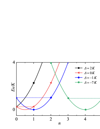
Figure 1: Eigenenergies of the Hamiltonian in Eq. (1) plotted as a function of photon number $n$ for drive $\beta=0$. The curves from left to right correspond to $\Delta/\text{K}=2$ (black), $0$ (red), $-1$ (blue), and $-7$ (green). The values of the energies are represented by symbols, which refer to integer value of $n$. The dashed lines are intended to show the degeneracy : $E_{0}=E_{1}$; $E_{0}=E_{2}$; $E_{3}=E_{5}$.

In the absence of the drive ($\beta=0$), the Hamiltonian in Eq. (1) can be diagonalized in the basis of Fock states (Zhang and Dykman, 2017), and the eigenvalues $E_{n}$ can be written in the following

$$E_{n}=\bar{E}_{n}-\bar{E}_{0},\ \bar{E}_{n}=K\left(n+\frac{\Delta}{2K}-\frac{1}{2}\right)^{2}.$$ (2)

From Eq. (2), for the integer $n$, $E_{n}$ is a simple parabola with a minimum at $n=1/2-\Delta/2K$ (see Fig.(1)). For $\Delta>0$, there is no degenerate in KNR. For $\Delta\leqslant 0$, the symmetrical eigenstates of $n=1/2-\Delta/2K$ will degenerate. Therefore, the ground state and degenerate states of KNR can be changed by adjusting the detuning $\Delta$.

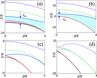
Figure 2: Eigenenergies of the Kerr nonlinearity resonator (KNR) plotted as functions of driving $\beta$ for different detuning $\Delta$. (a) $\Delta=0$, (b) $\Delta=2K$, (c) $\Delta=-K$, (d) $\Delta=-7K$. The Hamiltonian energy levels of even and odd parity are represented by solid and dashed lines, respectively.

For different detuning $\Delta$, the eigen energies of the KNR versus $\beta$ are shown in Fig. 2. A common trend is that, with large $\beta$, the Hamiltonian energy levels of the same parity repel each other, whereas adjacent energy levels with opposite parity attract each other and eventually merge together. When $\Delta\geqslant 0$, the vacuum state $|0\rangle$ and the first Fock state $|1\rangle$ are the two lowest energy states of the system, see Fig. 2(a) and Fig. 2(b). As the driving $\beta$ increases, they will degenerate to a new ground state. During the driving process, the minimum level gap $\Delta_{\text{min}}$ between the ground state and the first excited state is determined by $\Delta$. With increasing the detuning $\Delta$, the minimum level gap $\Delta_{\text{min}}$ will also increases.

When $\beta$ becomes larger than $\Delta$, the eigenstates of the system form many two-dimensional nearly degenerate subspace spanned by $\{D(\pm\alpha)|n\rangle\}$ for each $n$, where $\pm\alpha=\pm\sqrt{\beta/K}$ are the locations of the local maxima (Zhang and Dykman, 2017). The eigenstates of the system are two quasi-orthogonal states $|\psi^{\pm}_{n}\rangle=N^{\pm}[D(\alpha)\pm D(-\alpha)]|n\rangle$ with $N^{\pm}=1/\sqrt{2(1\pm e^{-2\alpha^{2}})}$, which are the even- and odd-parity states (Puri et al., 2019; Chamberland et al., 2020), marked by the red and blue levels respectively in Fig. 3. The cat states $|C^{\pm}_{\alpha}\rangle=N^{\pm}(|\alpha\rangle\pm|-\alpha\rangle)$ are degenerate ground state of the KNR in the limit of large $\beta$. As shown in Fig. 3, this degenerate cat state subspace (green) is separated from the rest of Hilbert space (orange) by a large energy gap $\Delta_{\text{gap}}$, which is well approximated as $\Delta_{\text{gap}}\sim 4K|\alpha|^{2}$ (Puri et al., 2020). For $\beta=0$, $|C^{+}_{\alpha}\rangle$ and $|C^{-}_{\alpha}\rangle$ are the vacuum state $|n=0\rangle$ and the first Fock state $|n=1\rangle$, respectively. Therefore, we can achieve the transition from the Fock state to the cat state by increasing the drive strength $\beta$.

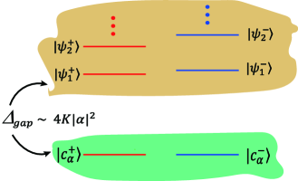
Figure 3: Eigenspectrum of the KNR in the limit of $\beta\gg\Delta,$ $K$. The eigenspectrum can be divided into an even (red) and an odd parity (green) manifold. The cat subspace (green) is separated from the rest of excited states (orange) by an energy gap $\Delta_{\text{gap}}\sim 4K|\alpha|^{2}$.

III Optimal Adiabatic control for preparing cat states

In this section, we introduce the optimal adiabatic control method to prepare cat states in the KNR. This method is based on quantum adiabatic theory, we first give a brief description of the QAT (Shankar, 2012; Aharonov and Anandan, 1987; Wu and Yang, 2005; Guéry-Odelin et al., 2019). If a system Hamiltonian is given by $H(C(t))$, where $C$ is some external coordinate which changes slowly and appears parametrically in $H$. The QAT shows that the probability of the system transition from the initial state $|m(0)\rangle$ to all $|n(t)\rangle(m\neq n)$ can be ignored, and the system will remain in the instantaneous eigenstate $|m(t)\rangle$ corresponding to the initial state. In this process, the quantum adiabatic condition

$$\left|\frac{\langle m(t)|\frac{\partial}{\partial t}|n(t)\rangle}{E_{m}(t)-E_{n}(t)}\right|\ll 1$$ (3)

must be satisfied, which means that the non-adiabatic transition between energy levels must be slow compared to the inverse energy gap between them. In Ref. (Aharonov and Anandan, 1987), the condition of the QAT is also summarized as

$$\left|\frac{\langle m(t)|\dot{H}|n(t)\rangle}{(E_{n}(t)-E_{m}(t))^{2}}\right|\ll 1,$$ (4)

which is equivalent to Eq. (3). The dot in Eq. (4) denotes the differentiation with respect to parameter $C$ and time $t$. The system adiabatic evolution time $T$ can be estimated from (Aharonov and Anandan, 1987)

$$T\gg\frac{1}{\Delta_{\text{min}}},$$ (5)

where $\Delta_{\text{min}}$ is the minimum energy level difference between the energy levels of the non-adiabatic transition. Therefore, in order to shorten the adiabatic evolution time $T$, it is necessary to increase the minimum energy level gap $\Delta_{\text{min}}$ of the system.

Then we give the initial conditions of the optimal adiabatic control method based on QAT. The system is initialized in the vacuum state $|0\rangle$ with initial drive strength $\beta_{0}=0$, and vary $\Delta$ and $\beta$ simultaneously to prepare the even cat state. The preparation of the odd cat state is same as the even cat state, except that the initial state of the system is prepared in Fock state $|1\rangle$. In the process of preparing the cat state, we should adiabatically keep the system in the ground state at all times to satisfy the adiabatic condition. According to the energy level structure of the KNR in section II, in the process of driving, the minimum energy gap $\Delta_{\text{min}}$ between the ground state and higher excited states decreases with increasing the initial detuning $\Delta$, as shown in Fig. 2(a) and 2(b). Therefore, we set the initial detuning $\Delta>0$ and assume it is time-dependent. In our proposal, $\beta$ ($\Delta$) increases (decreases) with time during the preparation of cat states.

Next, we determine the exact shape of the optimal adiabatic path. We parametrize the path as $C=\{\Delta(s),\beta(s):s\in[0,S]\}$, where $S$ is the total length of the path and define the small step length $ds$ in $(\Delta,\beta)$ space as $ds=\sqrt{(d\Delta)^{2}+(d\beta)^{2}}$. The trajectories of the parameters are obtained by introducing time dependence $s(t)$, which represents the distance covered up to time $t$. According to the condition for adiabaticity, an instantaneous penalty function $P_{C}(t)$ characterizing the probability of leaving the ground state is given by (Yanagimoto et al., 2019)

$$P_{C}(t)=\sum_{n\neq 0}\frac{|\langle\phi_{n}(t)|\frac{dH}{dt}|\phi_{0}(t)\rangle|}{|E_{n}(t)-E_{0}(t)|^{2}}=\frac{ds}{dt}Q_{C}(s).$$ (6)

Note that the time-dependent parameters in Eq. (6) are given via $s(t)$. Here, the function $Q_{C}$ is (Yanagimoto et al., 2019)

$$Q_{C}(s)=\sum_{n\neq 0}\frac{|\frac{d\beta}{ds}L_{n}(s)+\frac{d\Delta}{ds}M_{n}(s)|}{|E_{n}(s)-E_{0}(s)|^{2}},$$ (7)

with $|\phi_{n}(s)\rangle=|\phi_{n}(\Delta(s),\beta(s))\rangle$ and

$$L_{n}(s)=\langle\phi_{n}(s)|(a^{{\dagger}2}+a^{2})|\phi_{0}(s)\rangle,$$ (8)

$$M_{n}(s)=\langle\phi_{n}(s)|a^{{\dagger}}a|\phi_{0}(s)\rangle.$$ (9)

The total penalty of the path $C$ can be calculated by

$$I[C]=\int_{0}^{T}dtP_{C}(t)=\int_{0}^{S}dsQ_{C}(s),$$ (10)

where $T$ is the total time to traverse the path, so that $s(T)=S$. We then use the gradient-descent method to find a set of points that minimizes the second integral in the limited parameter space $\{\Delta,\beta\}$. By minimizing the second integral, we can determine the optimal path without preknowledge of $s(t)$.

Finally we choose the time dependence $s(t)$ to determine the optimal control sequence after obtaining an optimal path $C$. The penalty function $P$ is a non-negative function of time, so by Eq. (10),

$$\max_{t}P_{C}(t)\geqslant\frac{I[C]}{T}.$$ (11)

Choose a parametrization $P_{C}(t)=I[C]/T$, the inequality in Eq. (11) is always saturated (Yanagimoto et al., 2019). Under this choice, we have

$$t(s)=\frac{T}{I[C]}\int_{0}^{s}ds^{\prime}Q_{C}(s^{\prime}).$$ (12)

Through the numerically inverting $t(s)$, we obtain $s(t)$, which in turn generates the time-dependent trajectories of parameters $\beta(t)$ and $\Delta(t)$ and gives the total desired time $T$. Therefore, the optimal adiabatic control sequences for preparing cat state are obtained.

IV CAT-STATE GENERATION

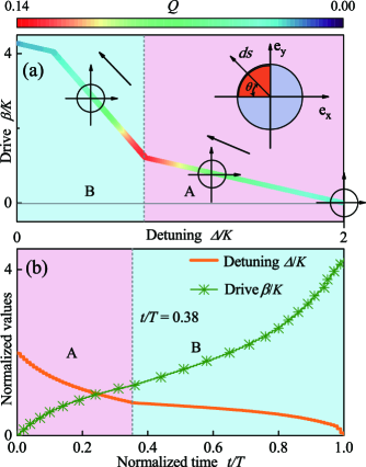
Figure 4: (a)By setting initial detuning $\Delta_{0}=2K$ and initial drive strength $\beta_{0}=0$ to generate the optimal path for preparing cat states. The color of path indicates the penalty $Q$ at each point. Arrows indicate the direction of gradient-descent. (b) Drive $\beta(t)$ and detuning $\Delta(t)$ as prescribed by Eq. (12) versus as $t$. Different background colors are used to represent the A and B regions.

In this section, we demonstrate generation of cat states via optimal adiabatic control method and show the advantages of this method. We initialize the system in the vacuum state $|0\rangle$ or the first Fock state $|1\rangle$ with initial detuning $\Delta_{0}=2K$ and initial drive strength $\beta_{0}=0$. For convenience, we set $K=1$ to determine the timescale in the following discussion. As shown in Fig. 4(a), we introduce the parameter $\theta$ and vector plane $(\vec{\mathbf{e}}_{x},\vec{\mathbf{e}}_{y})$, the small step with direction $d\vec{s}$ can be described by

$$\begin{aligned} d\vec{s}&=ds\ \text{cos}\theta\ \vec{\mathbf{e}}_{x}+ds\ \text{sin}\theta\ \vec{\mathbf{e}}_{y}\\ &=d\Delta\ \vec{\mathbf{e}}_{x}+d\beta\ \vec{\mathbf{e}}_{y},\end{aligned}$$ (13)

where $\theta\in(\pi/2,\pi)$ is determined by the changing trend of $\Delta$ and $\beta$. The parameters $\Delta$ and $\beta$ can be expressed as:

$$\begin{aligned} \Delta&=\Delta_{0}+d\Delta=2+ds\ \text{cos}\theta\\ \beta&=\beta_{0}+d\beta=0+ds\ \text{sin}\theta.\end{aligned}$$ (14)

To find the optimal route in parametric space $\{\Delta,\beta\}$, we need to determine $\theta$ corresponding to each step $ds$. This can be achieved by a numerical calculation based on gradient-descent method. Specifically, we first choose $(2,0)$ as the starting point, and make a circle with $(2,0)$ as the center and $ds$ as the radius. Then, we substitute all the points on the second quadrant of the circle into Eq. (7), and get a set of $Q_{C}(s_{0}+ds)$. We choose a $\theta$, which satisfies

$$\text{min}[Q_{C}(s_{0}+ds)-Q_{C}(s_{0})],$$ (15)

as the direction of gradient-descent. The position $s_{0}+ds$ is the point in the optimal path. We repeat the above process with the found point as the new starting point, until $\Delta$ is reduced to $0$ to stop the above process. The optimized path for preparing cat state with initial detuning $\Delta_{0}=2K$ and $\beta=0$ as shown in Fig. 4(a), the penalty function $Q_{C}$ at each point in our path satisfies the condition of adiabatic approximation $Q_{C}\ll 1$. We divide the optimized path into two regions according to the changing trend of penalty function $Q_{C}$ at each point, named A and B. The penalty function $Q_{C}$ for each point gradually increases in area A, and gradually decreases in area B.

To better understand the dynamics of this process, we use a displacement operator $D(\alpha)$ in our Hamiltonian of Eq. (1), where $D(\alpha)=\text{exp}(\alpha a^{{\dagger}}-\alpha^{\ast}a)$. Under a displacement transformation $D(\alpha)$, the system Hamiltonian becomes (Puri et al., 2017)

$$\begin{aligned} H^{\prime}=&D^{{\dagger}}(\alpha)HD(\alpha)\\ =&[(2K\alpha^{2}\alpha^{\ast}-2\beta\alpha^{\ast}+\Delta\alpha)a^{{\dagger}}+\text{H.c}]\\ &+[(K\alpha^{2}-\beta)a^{{\dagger}2}+\text{H.c}]+(4K|\alpha|^{2}+\Delta)a^{{\dagger}}a\\ &+Ka^{{\dagger}2}a^{2}+(2K\alpha a^{{\dagger}2}a+\text{H.c}),\end{aligned}$$ (16)

where we have dropped the constant term $E=4K|\alpha|^{4}-\beta(\alpha^{2}+(\alpha^{\ast})^{2})+\Delta|\alpha|^{2}$ that represents a shift in energy. We take $\alpha$ to satisfy (Puri et al., 2017)

$$2K\alpha^{2}\alpha^{\ast}-2\beta\alpha^{\ast}+\Delta\alpha=0,$$ (17)

such as to inhibit the the unwanted single-photon pumping. The Hamiltonian $H^{\prime}$ now reads

$$\begin{aligned} H^{\prime}=&[(K\alpha^{2}-\beta)a^{{\dagger}2}+\text{H.c}]+(4K|\alpha|^{2}+\Delta)a^{{\dagger}}a\\ &+Ka^{{\dagger}2}a^{2}+(2K\alpha a^{{\dagger}2}a+\text{H.c}).\end{aligned}$$ (18)

Equation (17) gives $\alpha=0,\pm\sqrt{(2\beta-\Delta)/2K}$, where we assume $\alpha=\alpha^{\ast}$.

For $\alpha=0$, the first two terms of Eq. (18) represent a nearly resonant parametric drive of strengh $\beta$ (Puri et al., 2017). When $\beta\ll\Delta$, the eigenstate of the system is approximately regarded as a Fock state. As the detuning $\Delta$ (drive strength $\beta$) continues to decrease (increase), the difference between $\Delta$ and $\beta$ decreases. However, the displaced amplitude $\alpha$ still very small, the instantaneous eigenstate of the system is still approximately regarded as a Fock state. The energy gap between the ground state and higher excited states is dominated by detuning $\Delta$. As $\Delta$ decreases, the probability of the ground state transitioning to higher excited states gradually increases. Therefore, the penalty function $Q_{C}$ that measures the transition probability will gradually increases with $\Delta$ decreases. The changing trend of the penalty function $Q_{C}$ is consistent with that in region A, which will increases with $\Delta$.

For $\alpha=\pm\sqrt{(2\beta-\Delta)/2K}$, the displaced Hamiltonian can be rewritten as (Puri et al., 2017)

$$\begin{aligned} H^{\prime}&=[(-\frac{\Delta}{2})a^{{\dagger}2}+\text{H.c}]+(4K|\alpha|^{2}+\Delta)a^{{\dagger}}a\\ &+Ka^{{\dagger}2}a^{2}+(2K\alpha a^{{\dagger}2}a+\text{H.c}).\end{aligned}$$ (19)

The first two terms of Eq. (19) now represent a parametric drive whose amplitude has an absolute value of $\Delta/2$, and is detuned by $4K|\alpha|^{2}+\Delta$. When $2\beta\gg\Delta$, the eigenstates of the system are spanned by $\{D(\pm\alpha)|n\rangle\}$ for each $n$, where $\pm\alpha=\pm\sqrt{(2\beta-\Delta)/2K}$. The probability of the ground state $D(+\alpha)|0\rangle$ transitioning to other excited sates $D(-\alpha)|n\rangle$ can be calculated by (Wang et al., 2019)

$$\langle n|D^{{\dagger}}(-\alpha)HD(+\alpha)|0\rangle\approx e^{-2\alpha^{2}}\approx e^{|(2\beta-\Delta)/K|}.$$ (20)

From Eq. (20), we find that the transition probability between the ground state and other excited states will decreases with $2\beta-\Delta$. The changing trend of the penalty function $Q_{C}$ in region B is consistent with Eq. (20), which will decreases with $2\beta-\Delta$.

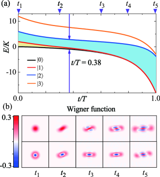
Figure 5: (a)Time evolution of the eigenenergies in the preparation of cat states adiabatically by adopting the optimal sequences $\{\Delta(t),\beta(t)\}$. (b) Wigner function $W(\alpha)$ at times $t_{1}$, $\dots$, $t_{5}$ shown on the top of panel (a). The first and second rows correspond to the initial state is vacuum state $|0\rangle$ and Fock state $|1\rangle$, respectively.

The optimal control sequence of detuning $\Delta(t)$ and driving strength $\beta(t)$ corresponding to each moment in the entire adiabatic evolution cycle is shown in Fig. 4(b). The detuning $\Delta(t)$ and drive strength $\beta(t)$ change faster in the A region, and gradually slow down in the B region. When detuning $\Delta$ decreases to zero, numerical solution indicates that the final pulse is $\beta_{f}=4.3K$. At $t=T$, the system evolves to target Hamiltonian

$$H=Ka^{{\dagger}}a^{{\dagger}}aa-\beta_{f}(a^{{\dagger}2}+a^{2}),$$ (21)

and can be re-written as (Wielinga and Milburn, 1993)

$$H=K(a^{{\dagger}2}-\beta_{f}/K)(a^{2}-\beta_{f}/K)-\beta_{f}^{2}/K.$$ (22)

This form of the Hamiltonian illustrate that two coherent states $|\pm\alpha\rangle$ with $\alpha=(\beta_{f}/K)^{1/2}$, which are degenerate eigenstates of Eq. (22) with energy $\beta_{f}^{2}/K$. Equivalently, the even-odd parity states $|C_{\alpha}^{\pm}\rangle$ are also the eigenstates of $H$. Therefore, after an adiabatic evolution cycle $T$, we obtain a cat state with amplitude $\sqrt{4.3}\approx 2.1$.

After acquiring the optimal control sequences $\{\Delta(t),\beta(t)\}$, we obtain the information of the entire evolution process. The eigenenergies of the ground, first, second and third instantaneous eigenstates are plotted in Fig. 5(a). Although the vacuum state $|0\rangle$ and the first Fock state $|1\rangle$ do not degenerate at the beginning, they will merge together and become the new ground state as the evolution time increases. However, the level gap between the vacuum state $|0\rangle$ or the Fock state $|1\rangle$ and higher excited state remains open throughout the entire adiabatic evolution cycle. This indicates that the adiabatic condition is always satisfied in the process of preparing cat states, and the system has always been in the ground state without transition to higher excited state. The changing trend of this energy gap is consistent with the penalty function $Q_{C}$ in Fig. 4(a), which decreases first and then gradually increases. When $t/\text{T}=0.38$, the energy gap will reach the minimum. We define this moment as $t_{\text{min}}$, which corresponds to the junction point of region A and region B in Fig. 4(a). We plot the simulated Wigner functions $W(\alpha)$ corresponding to the the instantaneous ground at different times in Fig. 5(b). After $t_{\text{min}}$, the system gradually transitions from the Fock state to the cat state. If the initial ground state of the system is a vacuum state $|0\rangle$, it will evolve into an even cat state $|C_{\alpha}^{+}\rangle$ at $t=T$. If the initial ground state of the system is the Fock sate $|1\rangle$, it will evolves to an odd cat state $|C_{\alpha}^{-}\rangle$ at $t=T$.

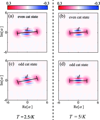
Figure 6: Wigner functions $W(\alpha)$ of final state for a KNR prepared by two-parameter-controlled (TPC) method and single-parameter-controlled (SPC) method, respectively. Where (a)(c) are TPC method, and (b)(d) are SPC method.

By tuning the two parameters of $\Delta$ and $\beta$, we successfully realize the preparation of cat states in KNR. In order to confirm the advantages of our two-parameter-controlled (TPC) method, we compare it with the single-parameter-controlled (SPC) method. The preparation of cat states is successfully achieved by adiabatic control of the two-photon pulsing $\{\beta\}$ in KNR in Ref. (Puri et al., 2017). Different from ours, their method sets the initial detuning $\Delta_{0}=0$, and only changes the two-photon drive strength $\beta$ adiabatically to achieve the preparation of cat states. The expression of their Hamiltonian is $H=Ka^{{\dagger}2}a^{2}-(\beta(t)a^{{\dagger}2}+\beta(t)^{*}a^{2})$, where drive strength $\beta(t)=\beta(t)^{*}=\beta_{0}[1-\text{exp}(-t^{4}/{T}^{4})]$. When $t\gg T$, $\beta(t)\sim\beta_{0}$, preparing the cat state with $\alpha=\sqrt{\beta_{0}/K}$. To prepare the same target state for these two methods, we set the driving constant $\beta_{0}=4.3K$. The adiabatic evolution time for preparing cat state in their method is $T=5/K$, and the adiabatic evolution time of our TPC method can be calculated according to Eq. (11), which is approximately as $T=2.5/K$.

Figure 6 shows the wigner functions $W(\alpha)$ in the finial state of the system after their respective adiabatic evolution cycles $T$. Both methods achieve the preparation of cat states, but the distance $d$ between the two coherent states $|\pm\alpha\rangle$ of the cat state prepared by our method is much farther. This means that cat states prepared by our method have larger size. Moreover, we also find that the interference fringes of the cat state prepared by our method are more clear than their method. This shows that cat states prepared by our method are more non-classical. By comparison, the TPC method prepares the cat state with larger size in a shorter time, and its non-classical features are better.

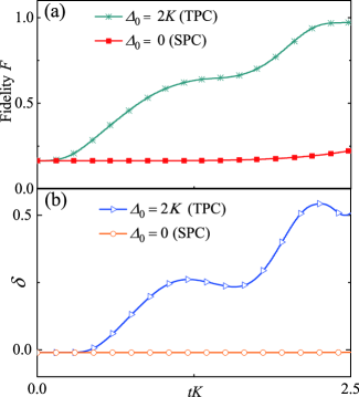
Figure 7: (Color online) Time evolution of the even cat state fidelity $F$ (a) and the nonclassicality volume $\delta$ (b) prepared by TPC and SPC methods .

For more convincing, we take the even cat state as an example to compare the fidelity $F$ and the non-classical volume $\delta$ of these two methods under the same evolution time $t$. We define the fidelity $F=\langle\Psi_{\alpha,\pm}|\rho(t)|\Psi_{\alpha,\pm}\rangle$, where $\Psi_{\alpha,\pm}=N^{-1/2}(|\alpha\rangle\pm|-\alpha\rangle)$ are the target cat states that these two methods aim to prepare with $\alpha=\sqrt{4.3}$. The non-classical volume $\delta$ is another important factor to evaluate the prepared cat state, which is defined as (Kenfack and Życzkowski, 2004)

$$\delta=\int|W(\alpha)|d^{2}\alpha-1.$$ (23)

A higher non-classical volume $\delta$ indicates more apparent non-classical features (Wang et al., 2017). Figure 7(a) compares the fidelity $F$ of these two methods under the same time $t$. At $t=2.5/K$, the fidelity of TPC method is about $98\%$, which is much greater than the SPC method. The comparison of the non-classical volumes $\delta$ of these two methods at the same evolution time is shown in Fig. 7(b). From $0$ to $t=2.5/K$, the non-classical volumes $\delta$ of TPC method increases rapidly, but $\delta$ of SPC method hardly changes. In the same evolutionary time $t$, the TPC method produces the cat state with a higher fidelity and a larger non-classical volume, which means that it is faster. The fast preparation of cat sate by this TPC method is due to the fact that the minimum energy gap $\Delta_{\text{min}}$ is increased by tuning additional detuning $\Delta$. In addition, the minimum energy gap $\Delta_{\text{min}}$ also affects the fidelity and the non-classical volume of prepared cat states. The larger $\Delta_{\text{min}}$, the smaller probability of the cat state transitioning to other excited states, and a higher fidelity and a larger non-classical volume cat state can be prepared.

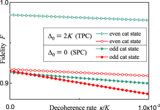
Figure 8: (Color online) The fidelity $F$ of the cat states prepared by SPC method and TPC method as a function of the single-photon loss rate $\kappa/K$.

Up to now, the discussions is based on the unitary evolution without considering decoherence. In order to generalize to the open-system case, we introduce a Lindblad jump operator $L=\sqrt{\kappa}a$ to describe the single-photon loss, and the dynamics of the system is described by the master equation

$$\dot{\rho}=-i[H,\rho]+L\rho L^{{\dagger}}-\frac{1}{2}L^{{\dagger}}L\rho-\frac{1}{2}\rho L^{{\dagger}}L.$$ (24)

In the presence of single-photon loss, the cat state parity will change randomly, reducing the fidelity of the prepared cat sate. We plot the fidelity $F$ of the cat states prepared by TPC and SPC methods respectively as a function of single-photon loss $\kappa$. The cat states prepared by these two methods are robust against single-photon loss very well. This is due to the fact that the two-photon driving $\beta$ can stabilize the cat state against the rotation and dephasing caused by Kerr nonlinearity (Puri et al., 2017). Here, we have not taken into account resonator dephasing and two-photon loss as they are typically negligible compared to single-photon loss (Puri et al., 2017).

V large scale cat states

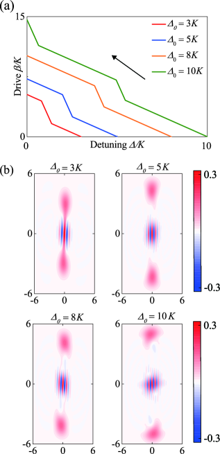
Figure 9: (a) Optimized path for generation cat states with different initial detuning $\Delta_{0}$. (b) Wigner functions $W(\alpha)$ of final state for KNR with different initial detuning $\Delta_{0}$.

Generally, cat states with $|\alpha|\geq 2$ can be treated as good qubits. Because two $|\pm\alpha\rangle$ of the cat state are not orthogonal with each other and their overlap is determined by $|\langle\alpha|-\alpha\rangle|=\text{exp}(-2|\alpha|^{2})$. For $|\alpha|\geq 2$, one has $|\langle\alpha|-\alpha\rangle|\approx 0$, and cat states can be used as cat bits. Hence, the preparation of large-size cat states plays an important role in continuously variable quantum information processing. Here, we will investigate the effect on the size of the prepared cat states when the initial detuning $\Delta_{0}$ takes a larger value. We adopt different $\Delta_{0}$ and discuss the effect of $\Delta_{0}$ on the size of the prepared cat state.

The optimal path for preparing cat states with different initial detuning $\Delta_{0}$ is shown in Fig. 9(a). We find that a large initial detuning $\Delta_{0}$ will lead to a large finial driving strength $\beta_{f}$. This means that the final Hamiltonian of the system can prepare cat state with large size. We plot the Wigner functions $W(\alpha)$ of the final cat states prepared by different initial $\Delta_{0}$ in Fig. 9(b)(the initial state is vacuum state $|0\rangle$). The result shows that with the increase of $\Delta_{0}$ , the distance $d$ between the two coherent states $|\pm\alpha\rangle$ gets farther, which also proves that the size of the cat state becomes larger. The interference fringes of Wigner functions in Fig. 9(b) are also clear, which means that the non-classical characteristics of cat states are also well. Therefore, we provide a method for preparing cat states with large-size.

VI possible realization with superconducting circuits

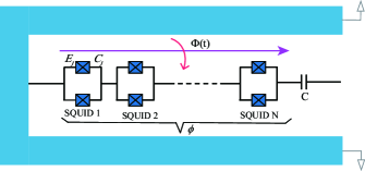
Figure 10: Schematic of a SQUID-array resonator with N SQUIDs. Each SQUID includes two identical Josephson junctions (with Josephson energy $E_{J}$ and capacitance $C_{J}$). The SQUID array is shunted by a shunting capacitor $C$, and the overall phase across the junction array is $\phi$. The external magnetic flux treading the SQUIDs is $\Phi(t)$.

As shown in Fig. 10, we dicuss how to realize our proposal by considering a SQUID-array resonator with N SQUIDs which has implemented in Refs. (Castellanos-Beltran and Lehnert, 2007; Castellanos-Beltran et al., 2008; Wang et al., 2019). The effective Hamiltonian of the system is given by (Wang et al., 2019)

$$\hat{H}=4E_{C}\hat{n}^{2}-NE_{J}[\Phi(t)]\text{cos}\frac{\hat{\phi}}{N},$$ (25)

where $\hat{n}$ and $\hat{\phi}$ are the number of Cooper pairs and the overall phase across the junction array, respectively. Here, $E_{C}$ is the resonator’s charging energy including the contributions of the junction capacitance $C_{J}$ and the shunt capacitance $C$. $N$ is the number of SQUIDs in the array. $E_{J}$ is the Josephson energy for a single SQUID in the array, which depends on the external flux $\Phi(t)$. The Josephson energy is periodically modulated by the external magnetic flux $\Phi(t)$, which expressed as $E_{J}+\delta E_{J}\text{cos}\omega_{p}t$.

After Taylor expanding $\text{cos}(\hat{\phi}/N)$ in Eq. (25) to fourth order, we obtain (Wang et al., 2019; Masuda et al., 2021)

$$\begin{aligned} \hat{H}/\hbar=\ &4E_{C}\hat{n}^{2}-NE_{J}(1-\frac{1}{2}(\frac{\hat{\phi}}{N})^{2}+\frac{1}{24}(\frac{\hat{\phi}}{N})^{4}+\dots)\\ &-N\delta E_{J}(1-\frac{1}{2}(\frac{\hat{\phi}}{N})^{2}+\dots)\text{cos}\omega_{p}t.\end{aligned}$$ (26)

The quadratic time-independent part of the Hamiltonian can be diagonalized by defining

$$\begin{aligned} &\hat{n}=-in_{0}(\hat{a}-\hat{a}^{{\dagger}}),\\ &\hat{\phi}=\phi_{0}(\hat{a}+\hat{a}^{{\dagger}}),\end{aligned}$$ (27)

where $n^{2}_{0}=\sqrt{E_{J}/32NE_{C}}$ and $\phi^{2}_{0}=\sqrt{2NE_{C}/E_{J}}$ are the zero-point fluctuations. After quantization, we obtain the Hamiltonian of the SQUID array resonator

$$\begin{aligned} \frac{\hat{H}}{\hbar}=\ &\omega^{(0)}_{c}(\hat{a}^{{\dagger}}\hat{a}+\frac{1}{2})+\frac{K}{6}(\hat{a}+\hat{a}^{{\dagger}})^{4}\\ &+[-\frac{N\delta E_{J}}{\hbar}-2\beta(\hat{a}+\hat{a}^{{\dagger}})^{2}-\frac{K\beta}{3\omega^{(0)}_{c}}(\hat{a}+\hat{a}^{{\dagger}})^{4}]\text{cos}\omega_{p}t,\end{aligned}$$ (28)

where $\omega_{c}^{(0)}=\sqrt{8E_{C}E_{J}/N}/\hbar$, $K=-E_{C}/N^{2}\hbar$ and $\beta=-\omega_{c}^{(0)}\delta E_{J}/8E_{J}$. Here, $K$ and $\beta$ corresponds to the Kerr nonlinearity coefficient and the pump strength, respectively. We consider a parameter regime in Eq. (25), where $\phi/N=2\sqrt{2K/\omega_{c}^{(0)}}$ is sufficiently smaller than unity. The last term in Eq. (28) can be neglected with an assumption, $K\beta\ll\omega_{c}^{(0)}$. Therefore, the Hamiltonian of the SQUID array resonator is achieved (Masuda et al., 2021)

$$\begin{aligned} \hat{H}/\hbar=\ &\omega^{(0)}_{c}\hat{a}^{{\dagger}}\hat{a}+\frac{K}{6}(\hat{a}+\hat{a}^{{\dagger}})^{4}-2\beta(\hat{a}+\hat{a}^{{\dagger}})^{2}\text{cos}\omega_{p}t.\end{aligned}$$ (29)

By moving into a rotating frame at the frequency of $\omega_{p}/2$ and performing a rotating-wave approximation (neglect all the rapidly oscillating terms), an approximate Hamiltonian can be obtained

$$\hat{H}/\hbar=K\hat{a}^{{\dagger}}\hat{a}^{{\dagger}}\hat{a}\hat{a}+\Delta\hat{a}^{{\dagger}}\hat{a}-\beta(\hat{a}^{2}+\hat{a}^{{\dagger}2}),$$ (30)

where the detuning $\Delta=\omega^{(0)}_{c}-2K-\omega_{p}/2$. This Hamiltonian has the same form as the Hamiltonian of Eq. (1), which can be used to prepare cat states.

VII conclusion

We propose a quantum speedup method to generate cat states in KNRs via optimal adiabatic control sequences. This method is based on gradient-descent, searching in a two-parameter space $\{\Delta,\beta\}$, and finds an optimal evolution path through numerical calculation. This TPC method offers a practical way to speed up the adiabatic evolution, which offers significant improvements over the previous SPC method. The results show that the cat state prepared by TPC method has a higher fidelity $F$ and a larger non-classical volume $\delta$ than SPC method at the same evolution time $t$. The cat states prepared by TPC method are also robust against single-photon loss very well. In addition, this TPC method also provides a promising solution to prepare a large-size cat state through a large initial detuning $\Delta_{0}$. We hope that these cat states can find wide applications in quantum information processing, especially in quantum information coding with cat states and quantum fault-tolerant computing.

References

References

- Zurek (2003) W. H. Zurek, Rev. Mod. Phys. 75, 715 (2003).
- Haroche (2013) S. Haroche, Rev. Mod. Phys. 85, 1083 (2013).
- Leggett and Garg (1985) A. J. Leggett and A. Garg, Phys. Rev. Lett. 54, 857 (1985).
- Yurke and Stoler (1986) B. Yurke and D. Stoler, Phys. Rev. Lett. 57, 13 (1986).
- Roy and Singh (1991) S. Roy and V. Singh, Phys. Rev. Lett. 67, 2761 (1991).
- Kim and Bužek (1992) M. Kim and V. Bužek, Phys. Rev. A 46, 4239 (1992).
- Shimizu and Miyadera (2002) A. Shimizu and T. Miyadera, Phys. Rev. Lett. 89, 270403 (2002).
- Shimizu and Morimae (2005) A. Shimizu and T. Morimae, Phys. Rev. Lett. 95, 090401 (2005).
- Morimae and Shimizu (2006) T. Morimae and A. Shimizu, Phys. Rev. A 74, 052111 (2006).
- Morimae (2010) T. Morimae, Phys. Rev. A 81, 010101 (2010).
- Fröwis and Dür (2012) F. Fröwis and W. Dür, New J. Phys. 14, 093039 (2012).
- Arndt and Hornberger (2014) M. Arndt and K. Hornberger, Nat. Phys. 10, 271 (2014).
- Fröwis et al. (2015) F. Fröwis, N. Sangouard, and N. Gisin, Opt. Commun. 337, 2 (2015).
- Jeong et al. (2015) H. Jeong, M. Kang, and H. Kwon, Opt. Commun. 337, 12 (2015).
- Fischer and Kang (2015) U. R. Fischer and M.-K. Kang, Phys. Rev. Lett. 115, 260404 (2015).
- Abad and Karimipour (2016) T. Abad and V. Karimipour, Phys. Rev. B 93, 195127 (2016).
- Lambert et al. (2016) N. Lambert, K. Debnath, A. F. Kockum, G. C. Knee, W. J. Munro, and F. Nori, Phys. Rev. A 94, 012105 (2016).
- Puri et al. (2019) S. Puri, A. Grimm, P. Campagne-Ibarcq, A. Eickbusch, K. Noh, G. Roberts, L. Jiang, M. Mirrahimi, M. H. Devoret, and S. M. Girvin, Phys. Rev. X 9, 041009 (2019).
- Mirrahimi et al. (2014) M. Mirrahimi, Z. Leghtas, V. V. Albert, S. Touzard, R. J. Schoelkopf, L. Jiang, and M. H. Devoret, New J. Phys. 16, 045014 (2014).
- Wang et al. (2016) C. Wang, Y. Y. Gao, P. Reinhold, R. W. Heeres, N. Ofek, K. Chou, C. Axline, M. Reagor, J. Blumoff, K. Sliwa, K. M. Sliwa, L. Frunzio, S. M. Girvin, L. Jiang, M. Mirrahimi, M. H. Devoret, and R. J. Schoelkopf, Science 352, 1087 (2016).
- Michael et al. (2016) M. H. Michael, M. Silveri, R. Brierley, V. V. Albert, J. Salmilehto, L. Jiang, and S. M. Girvin, Phys. Rev. X 6, 031006 (2016).
- Goto (2016a) H. Goto, Phys. Rev. A 93, 050301 (2016a).
- Wang et al. (2007) Z. Wang, C. Wu, X.-L. Feng, L. C. Kwek, C. Lai, C. H. Oh, and V. Vedral, Phys. Rev. A 76, 044303 (2007).
- Ma et al. (2021) W.-L. Ma, S. Puri, R. J. Schoelkopf, M. H. Devoret, S. Girvin, and L. Jiang, Sci. Bull. 66, 1789 (2021).
- Puri et al. (2020) S. Puri, L. St-Jean, J. A. Gross, A. Grimm, N. E. Frattini, P. S. Iyer, A. Krishna, S. Touzard, L. Jiang, A. Blais, et al., Sci. Adv. 6, eaay5901 (2020).
- Xu et al. (2021) Q. Xu, J. K. Iverson, F. G. Brandao, and L. Jiang, arXiv preprint arXiv:2105.13908 (2021).
- Vlastakis et al. (2013) B. Vlastakis, G. Kirchmair, Z. Leghtas, S. E. Nigg, L. Frunzio, S. M. Girvin, M. Mirrahimi, M. H. Devoret, and R. J. Schoelkopf, Science 342, 607 (2013).
- Leghtas et al. (2013a) Z. Leghtas, G. Kirchmair, B. Vlastakis, M. H. Devoret, R. J. Schoelkopf, and M. Mirrahimi, Phys. Rev. A 87, 042315 (2013a).
- Leghtas et al. (2013b) Z. Leghtas, G. Kirchmair, B. Vlastakis, R. J. Schoelkopf, M. H. Devoret, and M. Mirrahimi, Phys. Rev. Lett. 111, 120501 (2013b).
- Leghtas et al. (2015) Z. Leghtas, S. Touzard, I. M. Pop, A. Kou, B. Vlastakis, A. Petrenko, K. M. Sliwa, A. Narla, S. Shankar, M. J. Hatridge, et al., Science 347, 853 (2015).
- Ourjoumtsev et al. (2007) A. Ourjoumtsev, H. Jeong, R. Tualle-Brouri, and P. Grangier, Nature(London) 448, 784 (2007).
- Zhan et al. (2020) H. Zhan, G. Li, and H. Tan, Phys. Rev. A 101, 063834 (2020).
- Takahashi et al. (2008) H. Takahashi, K. Wakui, S. Suzuki, M. Takeoka, K. Hayasaka, A. Furusawa, and M. Sasaki, Phys. Rev. Lett. 101, 233605 (2008).
- Ourjoumtsev et al. (2006) A. Ourjoumtsev, R. Tualle-Brouri, J. Laurat, and P. Grangier, Science 312, 83 (2006).
- Wineland (2013) D. J. Wineland, Rev. Mod. Phys. 85, 1103 (2013).
- Sackett et al. (2000) C. A. Sackett, D. Kielpinski, B. E. King, C. Langer, V. Meyer, C. J. Myatt, M. Rowe, Q. Turchette, W. M. Itano, D. J. Wineland, et al., Nature(London) 404, 256 (2000).
- Leibfried et al. (2005) D. Leibfried, E. Knill, S. Seidelin, J. Britton, R. B. Blakestad, J. Chiaverini, D. B. Hume, W. M. Itano, J. D. Jost, C. Langer, et al., Nature(London) 438, 639 (2005).
- Hatomura (2018) T. Hatomura, New J. Phys. 20, 015010 (2018).
- Friedman et al. (2000) J. R. Friedman, V. Patel, W. Chen, S. Tolpygo, and J. E. Lukens, Nature(London) 406, 43 (2000).
- Van Der Wal et al. (2000) C. H. Van Der Wal, A. Ter Haar, F. Wilhelm, R. Schouten, C. Harmans, T. Orlando, S. Lloyd, and J. Mooij, Science 290, 773 (2000).
- Chen et al. (2021) Y.-H. Chen, W. Qin, X. Wang, A. Miranowicz, and F. Nori, Phys. Rev. Lett. 126, 023602 (2021).
- Wang et al. (2014) X. Wang, H.-r. Li, P.-b. Li, C.-w. Jiang, H. Gao, and F.-l. Li, Phys. Rev. A 90, 013838 (2014).
- Wang et al. (2017) X. Wang, A. Miranowicz, H.-R. Li, and F. Nori, Phys. Rev. B 95, 205415 (2017).
- Li et al. (2012) P.-B. Li, S.-Y. Gao, H.-R. Li, S.-L. Ma, and F.-L. Li, Phys. Rev. A 85, 042306 (2012).
- Wang and Clerk (2013) Y.-D. Wang and A. A. Clerk, Phys. Rev. Lett. 110, 253601 (2013).
- Qin et al. (2021) W. Qin, A. Miranowicz, H. Jing, and F. Nori, Phys. Rev. Lett. 127, 093602 (2021).
- Zhou et al. (2021) Z.-Y. Zhou, C. Gneiting, J. You, and F. Nori, Phys. Rev. A 104, 013715 (2021).
- Miranowicz et al. (1990) A. Miranowicz, R. Tanas, and S. Kielich, Quantum Opt. J. Eur. Opt. Soc. Part B 2, 253 (1990).
- Gu et al. (2017) X. Gu, A. F. Kockum, A. Miranowicz, Y.-x. Liu, and F. Nori, Phys. Rep. 718, 1 (2017).
- Dykman (2012) M. Dykman, Fluctuating nonlinear oscillators: from nanomechanics to quantum superconducting circuits (Oxford University Press, 2012).
- Siddiqi et al. (2005) I. Siddiqi, R. Vijay, F. Pierre, C. Wilson, L. Frunzio, M. Metcalfe, C. Rigetti, R. Schoelkopf, M. Devoret, D. Vion, et al., Phys. Rev. Lett. 94, 027005 (2005).
- Castellanos-Beltran et al. (2008) M. Castellanos-Beltran, K. Irwin, G. Hilton, L. Vale, and K. Lehnert, Nat. Phys. 4, 929 (2008).
- Munro et al. (2005) W. J. Munro, K. Nemoto, and T. P. Spiller, New J. Phys. 7, 137 (2005).
- Moloney and Newell (2018) J. Moloney and A. Newell, Nonlinear optics (CRC Press, 2018).
- Yin et al. (2012) Y. Yin, H. Wang, M. Mariantoni, R. C. Bialczak, R. Barends, Y. Chen, M. Lenander, E. Lucero, M. Neeley, A. O’Connell, et al., Phys. Rev. A 85, 023826 (2012).
- Zhao et al. (2018) P. Zhao, Z. Jin, P. Xu, X. Tan, H. Yu, and Y. Yu, Phys. Rev. Appl. 10, 024019 (2018).
- Goto (2016b) H. Goto, Sci. Rep. 6, 1 (2016b).
- Goto et al. (2019) H. Goto, Z. Lin, T. Yamamoto, and Y. Nakamura, Phys. Rev. A 99, 023838 (2019).
- Grimm et al. (2020) A. Grimm, N. E. Frattini, S. Puri, S. O. Mundhada, S. Touzard, M. Mirrahimi, S. M. Girvin, S. Shankar, and M. H. Devoret, Nature(London) 584, 205 (2020).
- Teh et al. (2020) R. Teh, F.-X. Sun, R. Polkinghorne, Q. He, Q. Gong, P. Drummond, and M. Reid, Phys. Rev. A 101, 043807 (2020).
- Sun et al. (2019) F.-X. Sun, Q. He, Q. Gong, R. Y. Teh, M. D. Reid, and P. D. Drummond, Phys. Rev. A 100, 033827 (2019).
- Lü et al. (2013) X.-Y. Lü, W.-M. Zhang, S. Ashhab, Y. Wu, and F. Nori, Sci. Rep. 3, 1 (2013).
- Kirchmair et al. (2013) G. Kirchmair, B. Vlastakis, Z. Leghtas, S. E. Nigg, H. Paik, E. Ginossar, M. Mirrahimi, L. Frunzio, S. M. Girvin, and R. J. Schoelkopf, Nature(London) 495, 205 (2013).
- Puri et al. (2017) S. Puri, S. Boutin, and A. Blais, NPJ Quantum Inf. 3, 1 (2017).
- Marthaler and Dykman (2007) M. Marthaler and M. Dykman, Phys. Rev. A 76, 010102 (2007).
- Zhang and Dykman (2017) Y. Zhang and M. Dykman, Phys. Rev. A 95, 053841 (2017).
- Chamberland et al. (2020) C. Chamberland, K. Noh, P. Arrangoiz-Arriola, E. T. Campbell, C. T. Hann, J. Iverson, H. Putterman, T. C. Bohdanowicz, S. T. Flammia, A. Keller, et al., arXiv preprint arXiv:2012.04108 (2020).
- Shankar (2012) R. Shankar, Principles of quantum mechanics (Springer Science & Business Media, 2012).
- Aharonov and Anandan (1987) Y. Aharonov and J. Anandan, Phys. Rev. Lett. 58, 1593 (1987).
- Wu and Yang (2005) Z. Wu and H. Yang, Phys. Rev. A 72, 012114 (2005).
- Guéry-Odelin et al. (2019) D. Guéry-Odelin, A. Ruschhaupt, A. Kiely, E. Torrontegui, S. Martínez-Garaot, and J. G. Muga, Rev. Mod. Phys. 91, 045001 (2019).
- Yanagimoto et al. (2019) R. Yanagimoto, E. Ng, T. Onodera, and H. Mabuchi, Phys. Rev. A 100, 033822 (2019).
- Wang et al. (2019) Z. Wang, M. Pechal, E. A. Wollack, P. Arrangoiz-Arriola, M. Gao, N. R. Lee, and A. H. Safavi-Naeini, Phys. Rev. X 9, 021049 (2019).
- Wielinga and Milburn (1993) B. Wielinga and G. Milburn, Phys. Rev. A 48, 2494 (1993).
- Kenfack and Życzkowski (2004) A. Kenfack and K. Życzkowski, J. Opt. B 6, 396 (2004).
- Castellanos-Beltran and Lehnert (2007) M. Castellanos-Beltran and K. Lehnert, Appl. Phys. Lett. 91, 083509 (2007).
- Masuda et al. (2021) S. Masuda, T. Ishikawa, Y. Matsuzaki, and S. Kawabata, Sci. Rep. 11, 1 (2021).