On the wave turbulence theory: ergodicity for the elastic beam wave equation

Abstract.

Inspiring by a recent work [57], we analyse a 3-wave kinetic equation, derived from the elastic beam wave equation on the lattice. The ergodicity condition states that two distinct wavevectors are supposed to be connected by a finite number of collisions. In this work, we prove that once the ergodicity condition is violated, the domain is broken into disconnected domains, called no-collision and collisional invariant regions. If one starts with a general initial condition, whose energy is finite, then in the long-time limit, the solutions of the 3-wave kinetic equation remain unchanged on the no-collision region and relax to local equilibria on the disjoint collisional invariant regions. The equilibration temperature will differ from region to region. This behavior of 3-wave systems was first described by Spohn in [55], without a detailed rigorous proof. Our proof follows Spohn’s physically intuitive arguments.

Keyword: wave turbulence, convergence to equilibrium, ergodicity condition, quadratic nonlinear Schrödinger equation.

1. Introduction

Having the origin in the works of Peierls [48, 49], Hasselmann [31, 32], Benney-Saffman-Newell [5, 6], Zakharov [61], wave kinetic equations have been shown to play important roles in a vast range of physical examples and this is why a huge and still growing number of situations have used WT theory: inertial waves due to rotation; Alfvén wave turbulence in the solar wind; waves in plasmas of fusion devices; and many others, as discussed in the books of Zakharov et.al. [61], Nazarenko [41] and the review papers of Newell and Rumpf [42, 43].

In rigorously deriving wave kinetic equations, the work of Lukkarinen and Spohn [40] for the cubic nonlinear Schödinger equation at equilibrium is pioneering. Works that rigorously derive the wave kinetic equations out of statistical equilibrium from the NLS equations with random initial data have been carried out by Buckmaster-Germain-Hani-Shatah [8, 9], Deng-Hani [17, 18], and Ampatzoglou-Collot-Germain [2, 14, 15]. Works that try to derive the 4-wave kinetic equation from the stochastic cubic nonlinear Schrödinger equation (NLS) have been written by Dymov, Kuksin and collaborators in [19, 20, 21, 22].

In a recent work by Staffilani-Tran in [57], the authors start from KdV type equations and derive the associated 3-wave kinetic equation rigorously. The method of proof is based on the use of Feynman diagrams and crossing estimates, under the observation that, most of the diagrams after being integrated out, produce positive powers $\lambda^{\theta},\theta>0$ of the small parameter $\lambda$ of the nonlinearity and hence become very small as $\lambda$ approaches $0$. The other diagrams are very special: they are self-repeated. The repeating structure was discovered the pioneering works of Erdos-Salmhofer-Yau for the Anderson model (see [24, 23]) and Lukkarinen-Spohn for the cubic nonlinear Schrödinger equation and other models (see [39, 40, 55, 56]). Let us also emphasize that in deriving kinetic equations from wave systems, the repeating structure and crossing estimates have a long history since the work of Erdos-Yau [11, 12, 13, 23, 24, 38, 40]. This repeating structure has been developed in combination with sophisticated crossing estimates and an analysis of the associated optimal transport equation, to study the KdV equation in [57].

We consider the quadratic elastic beam wave equation (Bretherton-type equation) (see Bretherton [7], Benney-Newell [4], Love [37])

$$\frac{\partial^{2}\psi}{\partial T^{2}}(x,T)\ +\ (\Delta+c)^{2}\psi(x,T)\ +\lambda\psi^{2}(x,T)\ =\ 0,$$ (1)

$$\psi(x,0) =\ \psi_{0}(x),\ \ \frac{\partial\psi}{\partial T}(x,0)\ =\ \psi_{1}(x),$$

for $x$ being on the torus $[0,1]^{3}$, $T\in\mathbb{R}_{+}$, $c\in\mathbb{R}$ is some real constant, $\lambda$ is a small constant describing the smallness of the nonlinearity. Equations of type (1) have been widely studied in control theory, and have been shown to have a Schrödinger structure (see, for instance, Burq [10], Fu-Zhang-Zuazua [26], Haraux [30], Lebeau [34], Lions [36], and Zuazua-Lions [62].) The analysis of (1) is also an interesting mathematical question of current interest (see, for instance, Hebey-Pausader [33], Levandosky-Strauss [35], Pausader [46] Pausader-Strauss [47].)

Performing a similar analysis with [57], we obtain the 3-wave kinetic equation

$$\partial_{t}f(k,t) =\ Q_{c}[f](k),\ \ \ \ f(k,0)\ =\ f_{0}(k),\ \ \forall k\in\mathbb{T}^{3},$$ (2)

$$Q_{c}[f](k) =\ \int_{\mathbb{T}^{6}}K(\omega,\omega_{1},\omega_{2})\delta(k-k_{1}-k_{2})\delta(\omega-\omega_{1}-\omega_{2})[f_{1}f_{2}-ff_{1}-ff_{2}]\mathrm{d}k_{1}\mathrm{d}k_{2}$$

$$-\ 2\int_{\mathbb{T}^{6}}K(\omega,\omega_{1},\omega_{2})\delta(k_{1}-k-k_{2})\delta(\omega_{1}-\omega-\omega_{2})[f_{2}f-ff_{1}-f_{1}f_{2}]\mathrm{d}k_{1}\mathrm{d}k_{2},$$

where $K(\omega,\omega_{1},\omega_{2})=[8\omega(k)\omega(k_{1})\omega(k_{2})]^{-1}$.

One of the main challenges in understanding the behaviors of solutions to the 3-wave kinetic equations is the so-called ergodicity, which is quite typical for 3-wave processes. Ergodicity has a long history in physics and we refer to [55][Section 17] for a more detailed discussion. To define ergodicity, we will need the concept of the connectivity between two wave vectors $k$ and $k^{\prime}$, which we briefly discuss here, leaving the precise definition for later. Given a wave vector $k$, a wave vector $k^{\prime}$ is understood to be connected to $k$ in a collision if either $\omega(k^{\prime})=\omega(k)+\omega(k^{\prime}-k)$, $\omega(k)=\omega(k^{\prime})+\omega(k-k^{\prime})$, or $\omega(k+k^{\prime})=\omega(k)+\omega(k^{\prime})$.

Ergodicity Condition (E): For every $k,k^{\prime}\in\mathbb{T}^{3}\backslash\{0\},$ there is a finite sequence of collisions such that $k$ is connected to $k^{\prime}$.

It was shown that (see [55]) under the Ergodicity Condition (E), the only stationary solutions of the spatially homogeneous Boltzmann equations (2) take the forms

$$\frac{1}{\beta\omega(k)},$$

in which $\beta$ can be computed via the conservation laws.

The aim of this work is to develop a rigorous analysis for the equations when the ergodicity condition is violated, to tackle the above problem. We will show that when the condition is violated, the domain of integration is broken into disconnected domains. There is one region, in which if one starts with any initial condition, the solutions remain unchanged as time evolves. In general, the equilibration temperature will differ from region to region. We call it the “no-collision region”. The rest of the domain is divided into disconnected regions, each has their own local equilibria, which are different in the classical and quantized cases. If one starts with any initial condition, whose energy is finite on one subdomain, the solutions will relax to the local equilibria of this subregion, as time evolves. Those subregions are named “collisional invariant regions”, due to the fact that we can rigorously establish unique local collisional invariants on each of them, using the conservation of energy and momenta. This confirms Spohn’s enlightening discussions [55] on the behavior of 3-wave systems.

Acknowledgements. B. R. is funded in part by a grant from the Simons Foundation (No. 430192). A. S. is in part by the Simons Foundation grant number 851844. M.-B. T is funded in part by the NSF Grant DMS-1854453, NSF RTG Grant DMS-1840260, URC Grant 2020, Humboldt Fellowship, Dedman College Linking Fellowship, NSF CAREER DMS-2044626. We would like to thank Prof. Herbert Spohn, Prof. Gigliola Staffilani and Prof. Enrique Zuazua for fruitful discussions on the topic.

2. From the Bretheton equation to the 3-wave kinetic equation

We follow the same strategy of Staffilani-Tran [57], and define the finite volume mesh

$$\Lambda\ =\ \Lambda(D)\ =\ \left\{0,\frac{1}{2D+1}\dots,\frac{2D}{2D+1}\right\}^{d},$$ (3)

for some constant $D\in\mathbb{N}$. Thus, the set $\Lambda$ is a subset of the $d$-dimensional torus $\left[0,1\right]^{d}$. We also define the mesh size to be

$$h^{d}=\left(\frac{1}{2D+1}\right)^{d}.$$ (4)

The discretized equation is now

$$\partial_{TT}\psi(x,T)\ = \ \ -\sum_{y\in\Lambda}O_{1}(x-y)\psi(y,T)\ -\ \lambda({\psi(x,T)})^{2},$$ (5)

$$\psi(x,0) =\ \psi_{0}(x),\ \partial_{T}\psi(x,0)\ =\ \psi_{1}(x),\ \forall(x,T)\in\Lambda\times\mathbb{R}_{+},$$

where $O_{1}(x-y)$ is a finite difference operator that we will express below in the Fourier space. We remark that a similar beam dynamics of non-acoustic chains has also been considered in [3][Section 7]. To obtain the lattice dynamics, we introduce the Fourier transform

$$\hat{\psi}(k)=h^{d}\sum_{x\in\Lambda}\psi(x)e^{-2\pi{\bf i}k\cdot x},\quad k\in\Lambda^{*}=\Lambda^{*}(D)=\{-D,\cdots,0,\cdots,D\}^{d},$$ (6)

at the end of this standard procedure, (5) can be rewritten in the Fourier space as a system of ODEs

$$\partial_{TT}\hat{\psi}(k,T)\ = \omega(k)^{2}\hat{\psi}(k,T)$$ (7)

$$\ -\lambda\sum_{k=k_{1}+k_{2};k_{1},k_{2}\in\Lambda^{*}}{\hat{\psi}(k_{1},T)}\hat{\psi}(k_{2},T),$$

$$\hat{\psi}(k,0) =\ \hat{\psi}_{0}(k),\ \ \ \partial_{T}\hat{\psi}(k,0)\ =\ \hat{\psi}_{1}(k),$$

where the dispersion relation takes the discretized form

$$\omega_{k}\ =\ \omega(k)\ =\ \sin^{2}(2\pi hk^{1})+\cdots+\sin^{2}(2\pi hk^{d})+c,$$ (8)

with $k=(k^{1},\cdots,k^{d})$.

We define the inverse Fourier transform to be

$$f(x)=\sum_{k\in\Lambda_{*}}\hat{f}(k)e^{2\pi{\bf i}k\cdot x}.$$ (9)

We also use the following notations

$$\int_{\Lambda}\mathrm{d}x\ =\ h^{d}\sum_{x\in\Lambda},\ \ \ \ \langle f,g\rangle\ =\ h^{d}\sum_{x\in\Lambda}f(x)^{*}g(x),$$ (10)

where if $z\in\mathbb{C}$, then $\bar{z}$ is the complex conjugate, as well as the Japanese bracket

$$\langle x\rangle\ =\ \sqrt{1+|x|^{2}},\ \ \forall x\in\mathbb{R}^{d}.$$ (11)

Moreover, for any $N\in\mathbb{N}\backslash\{0\}$, similar with [57], we define the delta function $\delta_{N}$ on $(\mathbb{Z}/N)^{d}$ as

$$\delta_{N}(k)=|N|^{d}\mathbf{1}(k\mbox{ mod }1\ =\ 0),\ \ \ \forall k\in(\mathbb{Z}/N)^{d}.$$ (12)

In our computations, we omit the sub-index $N$ and simply write

$$\delta(k)=|N|^{d}\mathbf{1}(k\mbox{ mod }1\ =\ 0),\ \ \ \forall k\in(\mathbb{Z}/N)^{d}.$$ (13)

Equation (7) can now be expressed as a coupling system

$$\frac{\partial}{\partial T}{q}(k,T) =\ {p}(k,T),$$ (14)

$$\frac{\partial}{\partial T}{p}(k,T) =\ \omega^{2}(k){q}(k,T)$$

$$\ \ \ \ -\lambda\int_{(\Lambda^{*})^{2}}\mathrm{d}k_{1}\mathrm{d}k_{2}\delta(k-k_{1}-k_{2}){q}(k_{1},T){q}(k_{2},T),$$

$$q(k,0) =\ \hat{\psi}_{0}(k),\ \ p(k,0)\ =\ \hat{\psi}_{1}(k),\ \ \ \ \forall(k,T)\in\Lambda^{*}\times\mathbb{R}_{+},$$

which, under the transformation (see [60])

$$a(k,T)\ =\ \frac{1}{\sqrt{2}}\Big{[}{\omega(k)}{q}(k,T)\ +\ \frac{i}{{\omega(k)}}{p}(k,T)\Big{]},$$ (15)

with the inverse

$${q}(k,T) =\ \frac{1}{\sqrt{2}\omega(k)}\Big{[}a(k)\ +\ a^{*}(k)\Big{]},$$ (16)

$${p}(k,T) =\ i\omega(k)\sqrt{\frac{1}{2}}\Big{[}-a(k)\ +\ a^{*}(-k)\Big{]},$$

leads to the following system of ordinary differential equations

$$\frac{\partial}{\partial T}a(k,T) =\ i\omega(k)a(k,T)\ -\ i\lambda\int_{(\Lambda^{*})^{2}}\mathrm{d}k_{1}\mathrm{d}k_{2}\delta(k-k_{1}-k_{2})\times$$ (17)

$$\times[8\omega(k)^{2}1\omega(k_{1})^{2}\omega(k_{2})^{2}]^{-\frac{1}{2}}\Big{[}a(k_{1},T)\ +\ a^{*}(-k_{1},T)\Big{]}\Big{[}a(k_{2},T)\ +\ a^{*}(-k_{2},T)\Big{]},$$

$$a(k,0) =\ a_{0}(k)\ =\ {\frac{1}{\sqrt{2}}\Big{[}{\omega(k)}{q}(k,0)\ +\ \frac{i}{{\omega(k)}}{p}(k,0)\Big{]}},\forall(k,T)\in\Lambda^{*}\times\mathbb{R}_{+}.$$

In order to absorb the quantity ${i}\sigma\omega(k)\hat{a}(k,\sigma,T)$ on the right hand side of the above system, we set

$$\alpha(k,T)\ =\ {a}(k,T)e^{-{i}\sigma\omega(k)T}.$$ (18)

The following system can be now derived for $\alpha_{T}(k)$

$$\frac{\partial}{\partial T}\alpha(k,T)\ =-\ {i}\sigma\lambda\sum_{k_{1},k_{2}\in\Lambda^{*}}\delta(k-k_{1}-k_{2})[8\omega(k)\omega(k_{1})\omega(k_{2})]^{-\frac{1}{2}}\times$$ (19)

$$\ \ \ \ \ \ \times\Big{[}\alpha(k_{1},T)\ +\ \alpha^{*}(-k_{1},T)\Big{]}\Big{[}\alpha(k_{2},T)\ +\ \alpha^{*}(-k_{2},T)\Big{]}e^{-{i}T\sigma(-\omega(k_{1})-\omega(k_{2})+\omega(k))}.$$

We also define

$$\sum_{k\in\Lambda^{*}}\ =\ \int_{\Lambda^{*}}\mathrm{d}k.$$ (20)

and perform the scaling

$$k^{\prime}=hk,\ \ \ \ a_{k}\to\breve{a}_{k^{\prime}}=\frac{a_{h^{-1}k^{\prime}}}{h^{d}},\ \ \ \ \alpha_{k}\to\breve{\alpha}_{k^{\prime}}=\frac{\alpha_{h^{-1}k^{\prime}}}{h^{d}},$$ (21)

and define the rescaled integrals

$$\int_{\mathrm{T}^{*}}\mathrm{d}k\ :=\ \frac{1}{|\Lambda^{*}|}\sum_{k\in\Lambda^{*}},$$ (22)

with

$$\mathrm{T}^{*}=\left\{-\frac{D}{2D+1},\cdots,0,\cdots,\frac{D}{2D+1}\right\}^{d},$$ (23)

to get

$$\frac{\partial}{\partial T}\breve{\alpha}(k,T)\ =-\ {i}\sigma\lambda\sum_{k_{1},k_{2}\in\mathrm{T}^{*}}\delta(k-k_{1}-k_{2})[8\omega(k)\omega(k_{1})\omega(k_{2})]^{-\frac{1}{2}}\times$$ (24)

$$\ \ \ \ \ \ \times\Big{[}\breve{\alpha}(k_{1},T)\ +\ \breve{\alpha}^{*}(-k_{1},T)\Big{]}\Big{[}\breve{\alpha}(k_{2},T)\ +\ \breve{\alpha}^{*}(-k_{2},T)\Big{]}e^{-{i}T\sigma(-\omega(k_{1})-\omega(k_{2})+\omega(k))}.$$

In this scaling, we set

$$\omega(k)\ =\ \sin^{2}(2\pi k^{1})+\cdots+\sin^{2}(2\pi k^{d})+c.$$ (25)

Consider the two-point correlation function

$$f_{\lambda,D}(k,T)\ =\ \langle\breve{\alpha}_{T}(k,-1)\breve{\alpha}_{T}(k,1)\rangle.$$ (26)

In the limit of $D\to\infty$, $\lambda\to 0$ and $T=\lambda^{-2}t=\mathcal{O}(\lambda^{-2})$, the two-point correlation function $f_{\lambda,D}(k,T)$ has the limit

$$\lim_{\lambda\to 0,D\to\infty}f_{\lambda,D}(k,\lambda^{-2}t)=f(k,t)$$

which solves the 3-wave equation (2).

The analysis of [55] and [57] can be repeated, to derive the 3-wave kinetic equation, leading to a formal derivation of the kinetic equation. Let us briefly recall the derivation of [57], which is done by expressing (LABEL:StartPoint:scale) in terms of a Duhamel expansion. By repeating this process $N$ times, one then obtains a multi-layer equation of $N$ Duhamel expansions. While performing this process, the time interval $[0,t]$ is divided into $N+1$ time slices $[0,s_{0}],$ $[s_{0},s_{0}+s_{1}]$, $\dots$, $[s_{0}+\cdots+s_{N-1},t]$ and $t=s_{0}+\cdots+s_{N}.$ The Duhamel expansions can be presented as Feynman diagrams, to be introduced below. The time slices are represented from the bottom to the top of the diagram, with the lengths $s_{0}$, $s_{1}$, $\dots$, $s_{N}$, as shown in Picture 1. At time slice $s_{i}$, the two momenta $k_{1},k_{2}$ are combined into the momentum $k$ in (LABEL:StartPoint:scale). This is represented on the diagram by the fact that at time slice $s_{i}$, there is exactly one couple of the segments of time slice $s_{i-1}$ fuses into one segment of time slice $s_{i}$. At the bottom of the graph, one adds cluster vertices indicating the delta functions $\delta(\sum_{l=1}^{m}k_{0,j_{l}})$, which come out naturally when one takes the expectations $\mathbb{E}(\prod_{l=1}^{m}a_{k_{0,j_{l}}})$ as the initial condition is randomized.

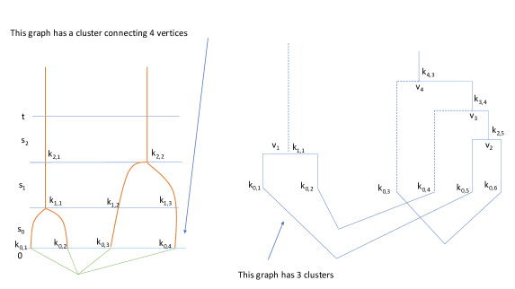
Figure 1. For the graph on the left, $k_{2,2}=k_{1,2}+k_{1,1}$ and $k_{1,1}=k_{0,1}+k_{0,2}$, these are the vertices where one applies the Duhamel expansions. For the graph on the right, the Duhamel expansions are applied at vertices $v_{1},v_{2},v_{3},v_{4}$. The graph on the left contains a cluster vertex that connects $4$ edges: $k_{0,1}+k_{0,2}+k_{0,3}+k_{0,4}=0$.

Most of the Feynman diagrams, after being integrated out, produce positive powers $\lambda^{\theta},\theta>0$ of the small parameter $\lambda$ and hence become very small as $\lambda$ approaches $0$. The other diagrams have very special structures: they are self-repeated. This repeating structure was first discovered for the Anderson model by Erdos-Salmhofer-Yau [24, 23] and for the cubic nonlinear Schrödinger equation as well as quantum fluids by Lukkarinen-Spohn [40, 39]. The structure has been adopted and developed, in combination with an analysis of the associated optimal transport equation, for the KdV equation in [57] (see Picture 2). The repeating structure of the quadratic Bretheton equation under consideration is precisely the one considered in [57]. Taking the limit $D\to\infty$ and summing all the recollisions in Figure 2, one obtains a solution to our 3-wave equation (1), yielding a formal derivation of the kinetic equation.

Remark 1.

It is discussed in [57] that the dispersion relation (8) is less troublesome the dispersion relation of the KdV equation, thus, the rigorous derivation of (1) should be similar but much simpler than the analysis performed in [57]. As the focus of our work is to confirm Spohn’s enlightening discussions in [55], we skip the rigorous derivation here.

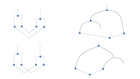
Figure 2. Examples of the repeating structures.

3. Main results

Let us first normalize the dispersion $\omega$ as

$$\omega(k)\ =\omega_{0}\ +\ \sum_{j=1}^{3}2\Big{(}1-\cos(2\pi k^{j})\Big{)},$$ (27)

where $2<\omega_{0}<3$, and $k=(k^{1},k^{2},k^{3})$.

For $\infty>m\geq 1$, let $\mathcal{S}$ be a Lebesgue measurable subset of $\mathbb{T}^{3}$ such that its measure is strictly positive, we introduce the function space ${L}^{m}(\mathcal{S})$, defined by the norm

$$\|f\|_{{L}^{m}(\mathcal{S})}:=\left(\int_{\mathcal{S}}|f(p)|^{m}\mathrm{d}p\right)^{\frac{1}{m}}.$$ (28)

In addition, we also need the space ${L}^{\infty}(\mathcal{S})$, defined by the norm

$$\|f\|_{{L}^{\infty}(\mathcal{S})}:=\mathrm{esssup}_{p\in\mathcal{S}}|f(p)|.$$ (29)

We denote by $C^{m}(\mathcal{S})$, $m=0,1,2,\dots$, the restrictions of all continuous and $m$-time differentiable functions on $\mathbb{T}^{3}$ onto $\mathcal{S}$. The space $C^{0}(\mathcal{S})=C(\mathcal{S})$ is endowed with the usual sup-norm (29). In addition, for any normed space $(Y,\|\cdot\|_{Y})$, we define

$$C([0,T),Y):=\Big{\{}F:[0,T)\to Y\;\big{|}F\mbox{ is continuous from $[0,T)$ to $Y$}\Big{\}}$$ (30)

and

$$C^{1}((0,T),Y):=\Big{\{}F:(0,T)\to Y\;\big{|}F\mbox{ is continuous and differentiable from $(0,T)$ to $Y$}\Big{\}},$$ (31)

for any $T\in(0,\infty]$. The above definitions can also be extended to the spaces $C([0,T],Y)$, $C^{1}((0,T],Y)$ for any $T\in(0,\infty)$.

Let us state our main theorem.

Theorem 2.

Under the assumption that there exists a positive, classical solution $f$ in $C([0,\infty),C^{1}(\mathbb{T}^{3}))\cap C^{1}((0,\infty),$ $C^{1}(\mathbb{T}^{3}))$ of (2), with the initial condition $f_{0}\in C(\mathbb{T}^{3})$, $f_{0}(k)\geq 0$ for all $k\in\mathbb{T}^{3}$.

The torus $\mathbb{T}^{3}$ can be decomposed into disjoint subsets as follows

$$\mathbb{T}^{3}\ =\ \mathfrak{I}\bigcup_{x\in\mathfrak{V}}\mathcal{S}(x),$$ (32)

where $\mathcal{S}(x)\cap\mathcal{S}(y)=\emptyset$ and $\mathcal{S}(x)\cap\mathfrak{I}=\emptyset$ for $x,y\in\mathfrak{V}$. The set $\mathfrak{I}$ is not empty and is called the “no-collision region”. The set $\mathcal{S}(x)$ is called the “collisional-invariant region”. For all $x\in\mathfrak{V}$, the Lebesgue measure $m(\mathcal{S}(x))$ of $\mathcal{S}(x)$ is strictly positive. The solution $f$ behaves differently on each sub-region.

• On $\mathfrak{I}$ the solution stays the same for all time

  $$f(t,k)=f_{0}(k),\ \ \ \ \forall t\geq 0,\ \ \ \ \forall k\in\mathfrak{I}.$$

• For all $x\in\mathfrak{V}$, let $(M_{x},E_{x})\in\mathbb{R}^{3}\times\mathbb{R}_{+}$ be a pair of admissible constants in the sense of Definition 1 below and assume further that they are indeed the local momenta and the local energy of the initial condition on $\mathcal{S}(x)$

  $$\int_{\mathcal{S}(x)}f_{0}(k)k\mathrm{d}k=M_{x},\ \ \ \ \int_{\mathcal{S}(x)}f_{0}(k)\omega(k)\mathrm{d}k=E_{x}.$$

  Suppose that the system of 4 equations with 4 variables $(a_{x},b_{x})\in\mathbb{R}_{+}\times\mathbb{R}^{3}$

  $$\int_{\mathcal{S}(x)}\frac{\omega(k)}{a_{x}\omega(k)+b_{x}\cdot k}\mathrm{d}k\ = \ E_{x},$$ (33)

  $$\int_{\mathcal{S}(x)}\frac{k}{a_{x}\omega(k)+b_{x}\cdot k}\mathrm{d}k\ = \ M_{x},$$

  has a unique solution $a_{x}\in\mathbb{R}_{+}$ and $b_{x}\in\mathbb{R}^{3}$ such that $a_{x}\omega(k)+b_{x}\cdot k>0$ for all $k\in\mathcal{S}(x)$; the local equilibrium on the collision invariant region $\mathcal{S}(x)$ can be uniquely determined as

  $$\frac{1}{a_{x}\omega(k)+b_{x}\cdot k}.$$ (34)

  Then, the following limits always holds true

  $$\lim_{t\to\infty}\left\|f(t,k)-\frac{1}{a_{x}\omega(k)+b_{x}\cdot k}\right\|_{L^{1}(\mathcal{S}(x))}=0.$$ (35)

  and

  $$\lim_{t\to\infty}\left|\int_{\mathcal{S}(x)}\ln[f]\mathrm{d}k-\int_{\mathcal{S}(x)}\ln\left[\frac{1}{a_{x}\omega(k)+b_{x}\cdot k}\right]\mathrm{d}k\right|=0.$$ (36)

  If, in addition, there is a positive constant $M^{*}>0$ such that $f(t,k)<M^{*}$ for all $t\in[0,\infty)$ and for all $k\in\mathcal{S}(x)$, then

  $$\lim_{t\to\infty}\left\|f(t,\cdot)-\frac{1}{a_{x}\omega(k)+b_{x}\cdot k}\right\|_{L^{p}(\mathcal{S}(x))}=0,\ \ \ \ \forall p\in[1,\infty).$$ (37)

  If we assume further that $f_{0}(k)>0$ for all $k\in\mathcal{S}(x)$, there exists a constant $M_{*}$ such that $f(t,k)>M_{*}$ for all $t\in[0,\infty)$ and for all $k\in\mathcal{S}(x)$.

Definition 1 (Admissible pairs of conservation constants).

Let $\mathcal{S}(x)$ be a collisional region.

• The pair $(E_{x},M_{x})$ of a constant $E_{x}\in\mathbb{R}_{+}$ and a vector $M_{x}\in\mathbb{R}^{3}$ is said to be admissible to be conservation constants in the classical sense if there exists a constant $\epsilon>0$ such that for all positive constant $E_{x}^{\prime}\in(E_{x}-\epsilon,E_{x}+\epsilon)$ and vector $M_{x}^{\prime}\in B(M_{x},\epsilon)$, the ball of $\mathbb{R}^{x}$ centered at $M_{x}$ with radius $\epsilon$, the system of $4$ equations with $4$ unknowns $a_{x}\in\mathbb{R}_{+}$ and $b_{x}\in\mathbb{R}^{3}$

  $$\int_{\mathcal{S}(x)}\frac{\omega(k)}{{a_{x}\omega(k)+b_{x}\cdot k}}\mathrm{d}k\ = \ E_{x}^{\prime},$$ (38)

  $$\int_{\mathcal{S}(x)}\frac{k}{{a_{x}\omega(k)+b_{x}\cdot k}}\mathrm{d}k\ = \ M_{x}^{\prime},$$

  has a unique solution $(a_{x},b_{x})$ such that $a_{x}\omega(k)+b_{x}\cdot k>0$ for all $k\in\mathcal{S}(x)$. In addition, $a_{x}$ and $b_{x}$ are continuous functions of $E_{x}^{\prime}$ and $M_{x}^{\prime}$.

• The pair $(E_{x},M_{x})$ of a constant $E_{x}\in\mathbb{R}_{+}$ and a vector $M_{x}\in\mathbb{R}^{3}$ is said to be admissible to be conservation constants in the quantized sense if there exists a constant $\epsilon>0$ such that for all positive constant $E_{x}^{\prime}\in(E_{x}-\epsilon,E_{x}+\epsilon)$ and vector $M_{x}^{\prime}\in B(M_{x},\epsilon)$, the ball of $\mathbb{R}^{x}$ centered at $M_{x}$ with radius $\epsilon$, the system of $4$ equations with $4$ unknowns $a_{x}\in\mathbb{R}_{+}$ and $b_{x}\in\mathbb{R}^{3}$

  $$\int_{\mathcal{S}(x)}\frac{\omega(k)}{e^{a_{x}\omega(k)+b_{x}\cdot k}-1}\mathrm{d}k\ = \ E_{x}^{\prime},$$ (39)

  $$\int_{\mathcal{S}(x)}\frac{k}{e^{a_{x}\omega(k)+b_{x}\cdot k}-1}\mathrm{d}k\ = \ M_{x}^{\prime},$$

  has a unique solution $(a_{x},b_{x})$ such that $a_{x}\omega(k)+b_{x}\cdot k>0$for all $k\in\mathcal{S}(x)$. In addition, $a_{x}$ and $b_{x}$ are continuous functions of $E_{x}^{\prime}$ and $M_{x}^{\prime}$.

Remark 3.

In the above theorem, we assume the well-posedness of the equation. As this piece of analysis is quite subtle and long, we reserve it for a separate paper.

Remark 4.

Notice that on the torus $\mathbb{T}^{3}$, the quantity $b\cdot k$ cannot show up, as discussed in [54], due to the periodicity and continuity of the equilibrium on $\mathbb{T}^{3}$. However, in the current situation, the local equilibrium is only defined on $\mathcal{S}(x)$, and not on the full $\mathbb{T}^{3}$. Indeed, the collision invariant regions $\mathcal{S}(x)$ belong to the interior of $\mathbb{T}^{3}$ and adding $b\cdot k$ does not violate the continuity and periodicity of the function on $\mathbb{T}^{3}$.

The above two theorems assert that those subregions are all non-empty. In the no-collision region $\mathfrak{I}$, any wavevector $k\in\mathfrak{I}$ is totally disconnected to other wavevectors, and thus the solutions on $\mathfrak{I}$ do not change as time evolves. In each of the collisional invariant regions $\mathcal{S}(x)$, as time goes to infinity, the solutions converge in the $L^{1}(\mathcal{S}(x))$-norm to $\frac{1}{a_{x}\omega(k)+b_{x}\cdot k}$ in the classical case and to $\frac{1}{e^{a_{x}\omega(k)+b_{x}\cdot k}-1}$ in the quantized case. In the classical case, to obtain the convergence, we need more regularity on the solutions: we assume that the solutions are in $C([0,\infty),C^{1}(\mathbb{T}^{3}))\cap C^{1}((0,\infty),$ $C^{1}(\mathbb{T}^{3}))$.

Let us also mention that this asymptotic behavior of the solutions to this 3-wave equations is very different from what is observed in spatially homogeneous and isotropic capillary or acoustic kinetic wave equations. It is showed in [53] that if one looks for a solution whose energy is a constant for all time to one of these isotropic capillary/acoustic kinetic wave equations, then this solution can exist only up to a finite time, after this time, some energy is lost to infinity. In other words, the solution exhibits the so-called energy cascade phenomenon.

4. The analysis of the 3-wave kinetic equation

In our proof, we suppose $K(\omega,\omega_{1},\omega_{2})$ is $[\omega(k)\omega_{1}(k)\omega_{1}(k)]^{-1}$ for the sake of simplicity.

4.1. No-collision, collisional regions and the 3-wave kinetic operator on these local disjoint sets

4.1.1. Collisional invariant regions

For a vector $x=(x^{1},x^{2},x^{3})\in\mathbb{T}^{3}$, we say that the wave vector $x$ is connected to the wave vector $y=(y^{1},y^{2},y^{3})\in\mathbb{T}^{3}$ by a forward collision if and only if

$$\mathfrak{F}^{f}_{x}(y)\ :=\ \sum_{j=1}^{3}2[\cos(2\pi(y_{j}-x_{j}))\ +\ \cos(2\pi x_{j})\ -\ \cos(2\pi y_{j})]\ -\ 6-\omega_{0}\ =\ 0.$$ (40)

In a forward collision, a particle with wave vector $y-x$ merges with a particle with wave vector $x$, resulting in a new particle with wave vector $y$. In this collision, the conservation of energy $\omega(y)=\omega(x)+\omega(y-x)$, describing by equation (40), needs to be satisfied. Therefore, given a particle with wave vector $x$, there maybe no wave vector $y$ such that the conservation of energy is guaranteed. In other words, there may be no $y$ such that $x$ is connected to $y$ by a forward collision.

On the other hand, we say that the wave vector $x$ is connected to the wave vector $y=(y^{1},y^{2},y^{3})\in\mathbb{T}^{3}$ by a backward collision if and only if

$$\mathfrak{F}^{b}_{x}(y)\ :=\ \sum_{j=1}^{3}2[\cos(2\pi y_{j})\ +\ \cos(2\pi(x_{j}-y_{j}))\ -\ \cos(2\pi x_{j})]\ -\ 6-\omega_{0}\ =\ 0.$$ (41)

Different from forward collisions, in a backward collision, a particle with wave vector $x$ is broken into two particles, one with wave vector $y$, and the other one with wave vector $x-y$. Again, in a backward collision, the conservation of energy $\omega(x)=\omega(y)+\omega(x-y)$ needs to be satisfied; and therefore, for a given wave vector $x$, it could happen that one cannot break $x$ into $y$ and $x-y$, such that the energy conservation (41) is satisfied.

Finally, we say that the wave vector $x$ is connected to the wave vector $y$ or the wave vector $y$ is connected to the wave vector $x$ by a central collision if and only if

$$\mathfrak{F}^{c}_{x}(y)\ =\ \mathfrak{F}^{c}_{y}(x)\ :=\ \sum_{j=1}^{3}2[\cos(2\pi y_{j})\ +\ \cos(2\pi(x_{j}))\ -\ \cos(2\pi(x_{j}+y_{j}))]\ -\ 6-\omega_{0}\ =\ 0.$$ (42)

Similarly to the above types of collisions, in a central collision, we require that $\omega(x)+\omega(y)=\omega(x+y)$ and this conservation of energy is not always satisfied.

Note that if $y$ is connected to $x$ by a forward collision, then $x$ is connected to $y$ by a backward collision. Moreover, if $y$ is connected to $x$ by a central collision, then $x$ is connected to $y$ by a central collision and $x+y$ is connected to both $x$ and $y$ by backward collisions. We simply say that $x$ and $y$ are connected by one collision; or $x$ is connected to $y$ and $y$ is connected to $x$ by one collision.

If a wave vector $k$ is not connected to any other wave vectors in forward collisions, the second term in the collision operator $Q_{c}[f](k)$

$$2\int_{\mathbb{T}^{6}}[\omega\omega_{1}\omega_{2}]^{-1}\delta(k_{1}-k-k_{2})\delta(\omega_{1}-\omega-\omega_{2})[f_{2}f-ff_{1}-f_{1}f_{2}]\mathrm{d}k_{1}\mathrm{d}k_{2}$$

vanishes, no matter how we choose the function $f$.

If a wave vector $k$ is not connected to any other wave vectors in backward collisions, the first term in the collision operator $Q_{c}[f](k)$

$$\int_{\mathbb{T}^{6}}[\omega\omega_{1}\omega_{2}]^{-1}\delta(k-k_{1}-k_{2})\delta(\omega-\omega_{1}-\omega_{2})[f_{1}f_{2}-ff_{1}-ff_{2}]\mathrm{d}k_{1}\mathrm{d}k_{2}$$

vanishes.

We define the set of all wave vectors $k$ such that $k$ is not connected to any other wave vectors to be the no-collision region $\mathfrak{I}$. It is clear that $\mathfrak{F}^{f}_{0}(y)=\mathfrak{F}^{c}_{0}(y)=-\omega_{0}<0$ and

$$\mathfrak{F}^{b}_{0}(y)=\sum_{j=1}^{3}2[2\cos(2\pi y_{j})-1]-6-\omega_{0}=\sum_{j=1}^{3}2[2\cos(2\pi y_{j})-2]-\omega_{0}\leq\ -\omega_{0}<0,$$

for all wave vectors $y$. As a consequence, the origin belongs to $\mathfrak{I}$. Since $\mathfrak{F}^{f}_{0}(y),\mathfrak{F}_{0}^{b}(y),\mathfrak{F}^{c}_{0}(y)\leq-\omega_{0}<0$, there exists a ball $B(0,R):=\{x\in\mathbb{R}^{3}\ \ |\ \ |x|<R\}$, $(R>0)$, such that $\mathfrak{F}^{f}_{x}(y),\mathfrak{F}_{x}^{b}(y),\mathfrak{F}^{c}_{x}(y)<0$, for all $y\in\mathbb{T}^{3}$ and for all $x\in B(0,R)$. The ball $B(0,R)$ is therefore a subset of the no-collision region $\mathfrak{I}$.

The condition $2<\omega_{0}<3$ implies that the set $\mathbb{T}^{3}\backslash\mathfrak{I}$ is then not empty. For a vector $x\in\mathbb{T}^{3}\backslash\mathfrak{I}$, we define $\mathcal{S}^{1}(x)$ to be the one-collision connection set of $x$, containing all wave vectors $y\in\mathbb{T}^{3}$ such that $y$ is connected to $x$ by a collision. By a recursive manner, we also define $\mathcal{S}^{n}(x)=\mathcal{S}^{1}(\mathcal{S}^{n-1}(x))$, the $n$-collision connection set of $x$, for $n\geq 2,n\in\mathbb{N}$. This set consists of all wave vectors connecting to $x$ by at most $n$ collisions. The union

$$\mathcal{S}(x)=\bigcup_{1\leq n<\infty}\mathcal{S}^{n}(x)$$ (43)

contains all wave vectors $y$ connecting to $x$ by a finite number of collisions. We then call $\mathcal{S}(x)$ a finite collision connection set of $x$ or a collision invariant region.

Note that if $k\in\mathcal{S}(x)$ and $k$ is connected to $k+k^{\prime}\in\mathcal{S}(x)$ by a forward collision, then $k+k^{\prime}$ is also connected with $k^{\prime}$ by a backward collision, and hence $k^{\prime}\in\mathcal{S}(x)$.

Proposition 5 (The effect of the collision operator on the no-collision region).

Any smooth solution $f(t,k)$ of (2), is time invariant on the no-collision region $\mathfrak{I}$. In other words, $f(t,k)=f_{0}(k)$ for all $k\in\mathfrak{I}$.

Proof.

Since $k\in\mathfrak{I}$, the wave vector $k$ is not connected to any other wave vectors in any collisions, the collision operator $Q_{c}[f](k)$ vanishes, which implies $\partial_{t}f(t,k)=0$ for all $k\in\mathfrak{I}$. Therefore, $f(t,k)=f_{0}(k)$ for all $k\in\mathfrak{I}$. ∎

Proposition 6 (Decomposition into collisional invariant regions).

Let $x,y$ be two wave vectors in $\mathbb{T}^{3}\backslash\mathfrak{I}$, then either $\mathcal{S}(x)=\mathcal{S}(y)$ or $\mathcal{S}(x)\cap\mathcal{S}(y)=\emptyset$. In other words, either $x$ and $y$ are connected by a finite number of collisions ($\exists m>0$ such that $x\in\mathcal{S}^{m}(y)$) or they are totally disconnected ($\nexists m>0$ such that $x\in\mathcal{S}^{m}(y)$).

As a consequence, there exists a subset $\mathfrak{V}$ of $\mathbb{T}^{3}\backslash\mathfrak{I}$ such that the torus $\mathbb{T}^{3}$ can be decomposed into disjoint collisional invariant regions, as follows

$$\mathbb{T}^{3}\backslash\mathfrak{I}\ =\ \bigcup_{x\in\mathfrak{V}}\mathcal{S}(x),$$ (44)

and $\mathcal{S}(x)\cap\mathcal{S}(y)=\emptyset$ for $x,y\in\mathfrak{V}$.

Proof.

Let $x,y$ be two wave vectors in $\mathbb{T}^{3}\backslash\mathfrak{I}$ and suppose that $\mathcal{S}(x)\cap\mathcal{S}(y)\neq\emptyset$, we can therefore choose a wave vector $z$ belonging to both sets $\mathcal{S}(x)$ and $\mathcal{S}(y)$, that means $z$ is connected to both wave vectors $x$ and $y$ by finite numbers of collisions. It follows that $z\in\mathcal{S}^{n}(x)$ and $z\in\mathcal{S}^{m}(y)$, for some positive integers $n$ and $m$. Since $z\in\mathcal{S}^{n}(x)$, it is clear that $\mathcal{S}(z)\subset\mathcal{S}^{n+1}(x)$, and in general $\mathcal{S}^{p}(z)\subset\mathcal{S}^{n+p}(x)$ for all $p\in\mathbb{N}$. As a result, $\mathcal{S}(z)\subset\mathcal{S}(x)$. By a similar argument, it also follows that $\mathcal{S}(z)\subset\mathcal{S}(y)$. Now, let $\vartheta$ be an wave vector of $\mathcal{S}(y)\backslash\mathcal{S}(z)$. Being a wave vector of $\mathcal{S}(y)$, $\vartheta$ is connected to $y$ by a finite number $p\in\mathbb{N}$ of collisions. Since $z$ is connected to $y$ by $m$ collisions, $\vartheta$ is connected to $z$ by at most $p+m$ collisions. In other words, $\vartheta\in\mathcal{S}^{p+m}(z)$; and hence, $\vartheta\in\mathcal{S}(z)$, contradicting the fact that $\vartheta\in\mathcal{S}(y)\backslash\mathcal{S}(z)$. This contradiction leads to $\mathcal{S}(y)\subset\mathcal{S}(z)$; however, as shown above $\mathcal{S}(z)\subset\mathcal{S}(y)$, it then follows $\mathcal{S}(y)=\mathcal{S}(z)$. The same argument can also be used to prove $\mathcal{S}(x)=\mathcal{S}(z)$. We finally get $\mathcal{S}(y)=\mathcal{S}(x)$.

The existence of $\mathfrak{V}$ and the decomposition (44) then follows straightforwardly. ∎

Remark 7.

The decomposition of the domain $\mathbb{T}^{3}$ in to several collisional invariant and no-collision regions is a very special and interesting feature of the specific form of the dispersion relation (27).

In the previous works, several other dispersion relations have been considered in many other contexts $\omega(k)=|k|$ for very low temperature bosons (see [1, 25]), $\omega(k)=|k|^{\gamma}$, $(1<\gamma\leq 2)$ for capillary waves (see [44]), $\omega(k)=\sqrt{c_{1}|k|^{2}+c_{2}|k|^{4}}$, $(0<c_{1},0\leq c_{2})$ for bosons (see [50, 52]). In all of these cases, the division of the domain of wavenumbers into disjoint regions has never been observed.

Notice that in [27], the dispersion relation $\omega(k)=\sqrt{c_{1}+c_{2}|k|^{2}}$, $(0<c_{1},c_{2})$ for stratified flows in the ocean, has been considered. However, the resonance is broadened and the extended resonance manifold is then studied

$$k=k_{1}+k_{2},\ \ \ |\omega(k)-\omega(k_{1})-\omega(k_{2})|\leq\theta,\ \ \ k,k_{1},k_{2}\in\mathbb{R}^{2},$$

for $\theta>0$, in stead of the standard resonance one

$$k=k_{1}+k_{2},\ \ \ \omega(k)=\omega(k_{1})+\omega(k_{2}),\ \ \ k,k_{1},k_{2}\in\mathbb{R}^{3},$$

due to some physical correctness (see [51]). Of course, in all resonance broadening cases, the decomposition of the full domain into local no-collision and collisional invariant regions does not exist.

Proposition 8.

The set $\mathcal{S}^{n}(x)$ is a closed subset of $\mathbb{T}^{3}$ for all $n\in\mathbb{N}\backslash\{0\}$.

Proof.

We first observe that the set $\mathcal{S}^{1}(x)$ contains all wave vectors $y$ such that $x$ is connected to $y$ by either a forward, a backward or a central collision. By definition, the set of all $y$ such that $x$ is connected to $y$ by a forward collision is

$$\mathcal{S}^{1}_{f}(x)\ =\ \left[\mathfrak{F}_{x}^{f}\right]^{-1}\left(\left\{0\right\}\right).$$ (45)

Similarly, the sets of all $y$ such that $x$ is connected to $y$ by backward and central collisions are

$$\mathcal{S}^{1}_{b}(x)\ =\ \left[\mathfrak{F}_{x}^{b}\right]^{-1}\left(\left\{0\right\}\right),$$ (46)

and

$$\mathcal{S}^{1}_{c}(x)\ =\ \left[\mathfrak{F}_{x}^{c}\right]^{-1}\left(\left\{0\right\}\right).$$ (47)

By the continuity of $\mathfrak{F}_{x}^{f},\mathfrak{F}_{x}^{b}$ and $\mathfrak{F}_{x}^{c}$, the sets $\mathcal{S}^{1}_{f}(x)$, $\mathcal{S}^{1}_{b}(x)$ and $\mathcal{S}^{1}_{c}(x)$ are all closed. Since $\mathcal{S}^{1}(x)=\mathcal{S}^{1}_{f}(x)\cup\mathcal{S}^{1}_{b}(x)\cup\mathcal{S}^{1}_{c}(x)$, it is also a closed set.

We now follow an induction argument in $n$. When $n=1$, it is clear from the above argument that $\mathcal{S}^{1}(x)$ is closed. Suppose that $\mathcal{S}^{k}(x)$ is closed, we will show that $\mathcal{S}^{k+1}(x)$ is also closed for all $k\geq 1$. To this end, let us suppose that $\{x_{m}\}_{m=1}^{\infty}$ is a sequence in $\mathcal{S}^{k+1}(x)$ and $\lim_{m\to\infty}x_{m}=x_{*}$. By the definition of the set $\mathcal{S}^{k+1}(x)$, there exists a sequence $\{y_{m}\}_{m=1}^{\infty}$ such that $y_{m}\in\mathcal{S}^{k}(x)$ and either $\mathfrak{F}^{f}_{y_{m}}(x_{m})=0$, $\mathfrak{F}^{b}_{y_{m}}(x_{m})=0$ or $\mathfrak{F}^{c}_{y_{m}}(x_{m})=0$. Without loss of generality, we can assume that there exist subsequences $\{x_{m_{q}}\}_{q=1}^{\infty}$ and $\{y_{m_{q}}\}_{q=1}^{\infty}$ of $\{x_{m}\}_{m=1}^{\infty}$ and $\{y_{m}\}_{m=1}^{\infty}$ such that $\mathfrak{F}^{f}_{y_{m_{q}}}(x_{m_{q}})=0$. Since the sequence $\{y_{m_{q}}\}_{q=1}^{\infty}$ is a subset of $\mathcal{S}^{k}(x)$, which is closed and hence compact, there exists a subset of $\{y_{m_{q}}\}_{q=1}^{\infty}$, still denoted by $\{y_{m_{q}}\}_{q=1}^{\infty}$, such that this sequence has a limit $y_{*}\in\mathcal{S}^{k}(x)$ as $q$ tends to infinity. By the continuity of $\mathfrak{F}^{f}_{y}(x)$ in both $x$ and $y$, $\lim_{q\to\infty}\mathfrak{F}^{f}{y_{m_{q}}}(x_{m_{q}})=\mathfrak{F}^{f}_{y_{*}}(x_{*})$. That implies $\mathfrak{F}^{f}_{y_{*}}(x_{*})=0$ and hence $x_{*}\in\mathcal{S}^{k+1}(x)$. We finally conclude that the set $\mathcal{S}^{k+1}(x)$ is closed. By induction $\mathcal{S}^{n}(x)$ is closed for all $n\in\mathbb{N}\backslash\{0\}$.

∎

Corollary 9.

The set $\mathcal{S}(x)$ is Lebesgue measurable.

Proof.

The proof of this corollary follows directly from Proposition 8 and the definition of $\mathcal{S}(x)$. ∎

Remark 10.

The two sets $\mathcal{S}^{1}_{f}(x)$ and $\mathcal{S}^{1}_{b}(x)$ defined in (45) and (46) are indeed disjoint. This can be seen by a proof of contradiction. Suppose that $y$ is a common wave vector of both $\mathcal{S}^{1}_{f}(x)$ and $\mathcal{S}^{1}_{b}(x)$. This means

$$\sum_{i=1}^{3}2[\cos(2\pi(y_{i}-x_{i}))+\cos(2\pi x_{i})-\cos(2\pi y_{i})]\ =\ 6+\omega_{0},$$

and

$$\sum_{i=1}^{3}2[\cos(2\pi(x_{i}-y_{i}))+\cos(2\pi y_{i})-\cos(2\pi x_{i})]\ =\ 6+\omega_{0}.$$

Taking the sum of the above two identities yields

$$\sum_{i=1}^{3}2\cos(2\pi(y_{i}-x_{i}))\ =\ 6+\omega_{0}.$$

The left hand side is smaller than or equal to $6$, while the right hand side is strictly greater than $6$ due to the fact that $\omega_{0}>0$. This leads to a contradiction; and thus, $\mathcal{S}^{1}_{f}(x)$ and $\mathcal{S}^{1}_{b}(x)$ are disjoint. However, $\mathcal{S}^{1}_{c}(x)$ can have common wave vectors with both $\mathcal{S}^{1}_{f}(x)$ and $\mathcal{S}^{1}_{b}(x)$.

Proposition 11.

The Lebesgue measure of $\mathcal{S}(x)$ is strictly positive.

Proof.

Let $x=(x^{1},x^{2},x^{3})$ and $y=(y^{1},y^{2},y^{3})$ be two wave vectors in $\mathcal{S}(x)$ satisfying

$$\omega_{0}\ +\ 6\ =\ \sum_{i=1}^{3}2[\cos(2\pi x^{i})\ +\ \cos(2\pi y^{i})-\ \cos(2\pi(x^{i}+y^{i}))].$$ (48)

For any numbers $\alpha,\beta\in\mathbb{T}$, define the function

$$\Upsilon(\alpha,\beta)\ :=\ \cos(2\pi\alpha)\ +\ \cos(2\pi\beta)-\ \cos(2\pi(\alpha+\beta)),$$ (49)

then it is straightforward that $-3\leq\Upsilon(\alpha,\beta)\leq\frac{3}{2}$.

For any number $\epsilon^{i}\in\mathbb{T},$ set

$$\delta_{i}(\epsilon^{i})\ := \ \cos(2\pi(y^{i}+\epsilon^{i}))\ -\ \cos(2\pi y^{i})\ -\ \cos(2\pi(x^{i}+y^{i}+\epsilon^{i}))\ +\ \cos(2\pi(x^{i}+y^{i}))$$ (50)

$$:= \Upsilon(x^{i},y^{i}+\epsilon^{i})-\Upsilon(x^{i},y^{i}),$$

for $i=1,2,3$. Taking the sum of the three functions $\delta_{i}(\epsilon^{i})$ yields

$$\sum_{i=1}^{3}\delta_{i}(\epsilon^{i})\ = \ \sum_{i=1}^{3}2[\cos(2\pi x^{i})\ +\ \cos(2\pi(y^{i}+\epsilon^{i}))-\ \cos(2\pi(x^{i}+y^{i}+\epsilon^{i}))]$$ (51)

$$- \ \sum_{i=1}^{3}2[\cos(2\pi x^{i})\ +\ \cos(2\pi y^{i})-\ \cos(2\pi(x^{i}+y^{i}))]$$

$$= \sum_{i=1}^{3}2[\Upsilon(x^{i},y^{i}+\epsilon^{i})-\Upsilon(x^{i},y^{i})].$$

We will show that for all $i=1,2,3$, $\Upsilon(x^{i},y^{i})>-3$. Suppose the contrary, that there is one $i\in\{1,2,3\}$ satisfying $\Upsilon(x^{i},y^{i})=-3$, then $\sum_{j\neq i}2\Upsilon(x^{j},y^{j})=\omega_{0}+12>12$, which contradicts the upper bound $\Upsilon(x^{j},y^{j})\leq\frac{3}{2}$. In addition, the case when $\Upsilon(x^{1},y^{1})=\Upsilon(x^{2},y^{2})=\Upsilon(x^{3},y^{3})=\frac{3}{2}$ will also not happen since $\omega_{0}<3$. Suppose, without loss of generality that $\Upsilon(x^{1},y^{1}),\Upsilon(x^{2},y^{2})>-3$ and $\Upsilon(x^{3},y^{3})<\frac{3}{2}$. By the continuity of $\Upsilon$, there exist intervals $I_{1},I_{2},I_{3}$ where $I_{i}$ can be either $[0,r^{i}]$ or $[-r^{i},0]$ for positive constant $r^{i}>0$, such that $-3<\Upsilon(x^{1},y^{1}+\epsilon^{1})<\Upsilon(x^{1},y^{1})$ for all $\epsilon^{1}\in I_{1}$, $-3<\Upsilon(x^{2},y^{2}+\epsilon^{2})<\Upsilon(x^{2},y^{2})$ for all $\epsilon^{2}\in I_{2}$ and $\frac{3}{2}>\Upsilon(x^{3},y^{3}+\epsilon^{3})>\Upsilon(x^{3},y^{3})$ for all $\epsilon^{3}\in I_{3}$.

Due to the continuity of $\delta^{i}$, we can choose $r^{i}$ small enough, $i=1,2,3$, such that for each pair $(\epsilon^{1},\epsilon^{2})\in I_{1}\times I_{2}$, there exists $\Omega(\epsilon^{1},\epsilon^{2})\in I_{3}$ satisfying $\delta_{1}(\epsilon^{1})+\delta_{2}(\epsilon^{2})+\delta_{3}(\Omega(\epsilon^{1},\epsilon^{2}))=0$. The function $\Omega(\epsilon^{1},\epsilon^{2})$ can be chosen to be continuous in the two variables $\epsilon^{1},\epsilon^{2}$ and $\Omega(0,0)=0.$ We then clearly have

$$\omega_{0}\ +\ 6\ = \ 2[\cos(2\pi x^{1})\ +\ \cos(2\pi(y^{1}+\epsilon^{1}))-\ \cos(2\pi(x^{1}+y^{1}+\epsilon^{1}))]$$ (52)

$$+\ 2[\cos(2\pi x^{2})\ +\ \cos(2\pi(y^{2}+\epsilon^{2}))-\ \cos(2\pi(x^{2}+y^{2}+\epsilon^{2}))]$$

$$+\ 2[\cos(2\pi x^{3})\ +\ \cos(2\pi(y^{3}+\Omega(\epsilon^{1},\epsilon^{2})))-\ \cos(2\pi(x^{3}+y^{3}+\Omega(\epsilon^{1},\epsilon^{2}))],$$

for all $(\epsilon_{1},\epsilon_{2})\in I_{1}\times I_{2}$. We deduce from this identity that the wave vector $(y^{1}+\epsilon^{1},y^{2}+\epsilon^{2},y^{3}+\Omega(\epsilon^{1},\epsilon^{2}))$ is connected to the wave vector $x$ by a central collision.

For all $(\epsilon_{1},\epsilon_{2})\in I_{1}\times I_{2}$ and $\theta^{1},\theta^{2},\theta^{3}\in\mathbb{T},$ define

$$\Delta_{1}(\epsilon^{1},\theta^{1})\ := \ \cos(2\pi(x^{1}+\theta^{1}))-\ \cos(2\pi x^{1})\$$ (53)

$$-\ \cos(2\pi(x^{1}+y^{1}+\epsilon^{1}+\theta^{1}))\ +\ \cos(2\pi(x^{1}+y^{1}+\epsilon^{1})),$$

$$\Delta_{2}(\epsilon^{2},\theta^{2})\ := \ \cos(2\pi(x^{2}+\theta^{2}))-\ \cos(2\pi x^{2})\$$

$$-\ \cos(2\pi(x^{2}+y^{2}+\epsilon^{2}+\theta^{2}))\ +\ \cos(2\pi(x^{2}+y^{2}+\epsilon^{2})),$$

$$\Delta_{3}(\Omega(\epsilon^{1},\epsilon^{2}),\theta^{3})\ := \ \cos(2\pi(x^{3}+\theta^{3}))-\ \cos(2\pi x^{3})\$$

$$-\ \cos(2\pi(x^{3}+y^{3}+\Omega(\epsilon^{1},\epsilon^{2})+\theta^{3}))\ +\ \cos(2\pi(x^{3}+y^{3}+\Omega(\epsilon^{1},\epsilon^{2})).$$

The same argument as above can also be applied, for each fixed $(\epsilon^{1},\epsilon^{2},\Omega(\epsilon^{1},\epsilon^{2}))\in I_{1}\times I_{2}\times I_{3}$. That leads to the existence of intervals $I_{4},I_{5},I_{6}$ where $I_{i}$ can be either $[0,r^{i}]$ or $[-r^{i},0]$ for positive constant $r^{i}>0$, such that for each pair $(\theta^{1},\theta^{2})\in I_{4}\times I_{5}$, there exists $\Theta(\epsilon^{1},\epsilon^{2})\in I_{6}$ satisfying $\Delta_{1}(\epsilon^{1},\theta^{1})+\Delta_{2}(\epsilon^{2},\theta^{2})+\Delta_{3}(\Omega(\epsilon^{1},\epsilon^{2}),\Theta(\theta^{1},\theta^{2}))=0$. Similarly, $\Theta$ is a continuous function of the two variables $\theta^{1},\theta^{2}$ and $\Theta(0,0)=0.$ If $\frac{3}{2}>\Upsilon(x^{1},y^{1}),\Upsilon(x^{2},y^{2}),\Upsilon(x^{3},y^{3})$, the intervals $I_{1}$, $I_{2}$, $I_{3}$ and $I_{4}$ can be chosen such that $I_{3}\subset I_{1}$ and $I_{4}\subset I_{2}$. If there is an index $j\in\{1,2,3\}$ such that $\Upsilon(x^{j},y^{j})=\frac{3}{2}$, then $x^{j}=y^{j}=\frac{1}{6}$, the intervals $I_{1}$, $I_{2}$, $I_{3}$ and $I_{4}$ can still be chosen such that $I_{3}\subset I_{1}$ and $I_{4}\subset I_{2}$. In addition, by taking $r^{1},r^{2}$ smaller, we can guarantee that $I_{1}=I_{3}$ and $I_{2}=I_{4}$. The following identity then follows

$$\omega_{0}\ +\ 6\ = \ 2[\cos(2\pi(x^{1}+\theta^{1}))\ +\ \cos(2\pi(y^{1}+\epsilon^{1}))-\ \cos(2\pi(x^{1}+y^{1}+\theta^{1}+\epsilon^{1}))]$$ (54)

$$+\ 2[\cos(2\pi(x^{2}+\theta^{2}))\ +\ \cos(2\pi(y^{2}+\epsilon^{2}))-\ \cos(2\pi(x^{2}+y^{2}+\theta^{2}+\epsilon^{2}))]$$

$$+\ 2[\cos(2\pi(x^{3}+\Theta(\theta^{1},\theta^{2})))\ +\ \cos(2\pi(y^{3}+\Omega(\epsilon^{1},\epsilon^{2})))$$

$$-\ \cos(2\pi(x^{3}+y^{3}+\Omega(\epsilon^{1},\epsilon^{2})+\Theta(\theta^{1},\theta^{2})))],$$

for all $\epsilon^{1},\theta^{1}\in I_{1}$, $\epsilon^{2},\theta^{2}\in I_{2}$.

Now, we will show that there exists a pair $(\rho_{1},\rho_{2})\in(I_{1}+I_{1})\times(I_{2}+I_{2})$ (recall that we have made $r^{1},r^{2}$ smaller, to have $I_{1}=I_{3}$ and $I_{2}=I_{4}$), such that the closed set

$$A_{(\rho_{1},\rho_{2})}=\Big{\{}\Omega(\epsilon^{1},\epsilon^{2})+\Theta(\rho_{1}-\epsilon^{1},\rho_{2}-\epsilon^{2}),\ \ \ \ \forall(\epsilon^{1},\epsilon^{2})\in I_{1}\times I_{2}\Big{\}},$$ (55)

does not reduce to a single point. This can be easily seen by a proof of contradiction with the assumption that for all $(\rho_{1},\rho_{2})\in(I_{1}+I_{1})\times(I_{2}+I_{2})$, the set $A_{(\rho_{1},\rho_{2})}$ contains only one point. For $(\epsilon^{1},\epsilon^{2})=(0,0)$, since $\Omega(0,0)=0$, it follows that $\Omega(0,0)+\Theta(\rho_{1},\rho_{2})=\Theta(\rho_{1},\rho_{2})\in A_{(\rho_{1},\rho_{2})}.$ For $(\epsilon^{1},\epsilon^{2})=(\rho_{1},\rho_{2})$, since $\Theta(0,0)=0$, it also follows that $\Theta(0,0)+\Omega(\rho_{1},\rho_{2})=\Omega(\rho_{1},\rho_{2})\in A_{(\rho_{1},\rho_{2})}.$ Since $A$ contains only one point, it is clear that $\Omega(\rho_{1},\rho_{2})=\Theta(\rho_{1},\rho_{2})$ for all $(\rho_{1},\rho_{2})\in(I_{1}+I_{1})\times(I_{2}+I_{2})$. The set $A_{(\rho_{1},\rho_{2})}$ becomes

$$A_{(\rho_{1},\rho_{2})}=\Big{\{}\Omega(\epsilon^{1},\epsilon^{2})+\Omega(\rho_{1}-\epsilon^{1},\rho_{2}-\epsilon^{2}),\ \ \ \ \forall(\epsilon^{1},\epsilon^{2})\in I_{1}\times I_{2}\Big{\}}=\{\Omega(\rho_{1},\rho_{2})\},$$ (56)

which implies $\Omega(\epsilon^{1},\epsilon^{2})+\Omega(\rho_{1}-\epsilon^{1},\rho_{2}-\epsilon^{2})=\Omega(\rho_{1},\rho_{2})$ for all $(\epsilon^{1},\epsilon^{2}),(\rho_{1}-\epsilon^{1},\rho_{2}-\epsilon^{2})\in I_{1}\times I_{2}$. Choosing $\epsilon^{2}=\rho_{2}=0$ yields $\Omega(\epsilon^{1},0)+\Omega(\rho_{1}-\epsilon^{1},0)=\Omega(\rho_{1},0)$, which means $\Omega(\rho_{1},0)=\Theta(\rho_{1},0)=C\rho_{1}$, where $C$ is a universal constant. This function does not satisfies (54) no matter what choice of the constant $C$ is. In other words, there exists $(\rho_{1},\rho_{2})\in(I_{1}+I_{1})\times(I_{2}+I_{2})$ such that the closed set $A_{(\rho_{1},\rho_{2})}$ contains a closed interval $[\gamma_{1},\gamma_{2}]$.

Since $x+y+(\theta^{1}+\epsilon^{1},\theta^{2}+\epsilon^{2},\Omega(\epsilon^{1},\epsilon^{2})+\Theta(\rho_{1}-\epsilon^{1},\rho_{2}-\epsilon^{2}))$ is connected to $(y^{1}+\epsilon^{1},y^{2}+\epsilon^{2},y^{3}+\Omega(\epsilon^{1},\epsilon^{2}))$ by a backward collision. The above argument shows the existence of two numbers $\rho_{1},\rho_{2}$ and an interval $[\gamma_{1},\gamma_{2}]$ such that for any $\zeta\in[\gamma_{1},\gamma_{2}]$ the wave vector $x+y+(\rho_{1},\rho_{2},\zeta)$ is connected to $x$ by at most 2 collisions.

Due to the continuity of the function $\Omega(\epsilon^{1},\epsilon^{2})+\Theta(\rho_{1}-\epsilon^{1},\rho_{2}-\epsilon^{2})$, there exist intervals $J_{1},J_{2}$, $I_{1}^{\prime},I_{2}^{\prime}$, $J^{*}$ such that $\epsilon^{1}\in I_{1}^{\prime}\subset I_{1}$, $\epsilon^{2}\in I_{2}^{\prime}\subset I_{2}$, $J_{1}\times J_{2}\subset(I_{1}+I_{1})\times(I_{2}+I_{2})$, $J^{*}\subset[\gamma_{1},\gamma_{2}]$. In addition, for each $\rho_{1}^{\prime}\in J_{1}$, $\rho_{2}^{\prime}\in J_{2}$ and $\xi\in J^{*}$, there exists $\epsilon^{1}_{0}\in I_{1}^{\prime},$ $\epsilon^{2}_{0}\in I_{2}^{\prime},$ such that $\xi=\Omega(\epsilon^{1}_{0},\epsilon^{2}_{0})+\Theta(\rho_{1}^{\prime}-\epsilon^{1}_{0},\rho_{2}^{\prime}-\epsilon^{2}_{0})$. Hence, the wave vector $x+y+(\rho_{1}^{\prime},\rho_{2}^{\prime},\Omega(\epsilon^{1}_{0},\epsilon^{2}_{0})+\Theta(\rho_{1}^{\prime}-\epsilon^{1}_{0},\rho_{2}^{\prime}-\epsilon^{2}_{0}))$ is connected to $(y^{1}+\epsilon^{1}_{0},y^{2}+\epsilon^{2}_{0},y^{3}+\Omega(\epsilon^{1}_{0},\epsilon^{2}_{0}))$ by a backward collision. Since the wave vector $(y^{1}+\epsilon^{1}_{0},y^{2}+\epsilon^{2}_{0},y^{3}+\Omega(\epsilon^{1}_{0},\epsilon^{2}_{0}))$ is connected to the wave vector $x$ by a central collision, it follows that the wave vector $x+y+(\rho_{1}^{\prime},\rho_{2}^{\prime},\Omega(\epsilon^{1}_{0},\epsilon^{2}_{0})+\Theta(\rho_{1}^{\prime}-\epsilon^{1}_{0},\rho_{2}^{\prime}-\epsilon^{2}_{0}))$ is connected to the wave vector $x$ by at most two collisions. Thus, for any $(\zeta_{1},\zeta_{2},\zeta_{3})\in J_{1}\times J_{2}\times J^{*},$ the vector $x+y+(\zeta_{1},\zeta_{2},\zeta_{3})$ belongs to $\mathcal{S}(x)$. Therefore the Lebesgue measure $m(\mathcal{S}(x))$ of $\mathcal{S}(x)$ satisfies the inequality $m(\mathcal{S}(x))\geq m(J_{1}\times J_{2}\times J^{*})>0$. This finishes our proof of the Proposition. ∎

4.1.2. Nonnegativity, countable additivity, uniqueness, boundedness of set index functionals

In the study of the wave kinetic equation, we frequently encounter integrals of the types

$$\int_{\mathbb{T}^{3}}\delta(\omega(x)-\omega(x-y)-\omega(y))f(y)\mathrm{d}y,$$ (57)

$$\int_{\mathbb{T}^{3}}\delta(\omega(y)-\omega(y-x)-\omega(x))f(y)\mathrm{d}y,$$ (58)

and

$$\int_{\mathbb{T}^{3}}\delta(\omega(x+y)-\omega(x)-\omega(y))f(y)\mathrm{d}y.$$ (59)

Special cases of (57)-(58)-(59) involve $f(y)=\chi_{A}(y)$, the characteristic function of a Lebesgue measurable set $A$. This section is devoted to the study of various important properties of the following index functionals of a measurable set $A$.

Definition 2 (Index functionals of sets).

Let $A$ be a Lebesgue measurable set, we define the following three functionals.

• The “forward collision” index of the set $A$:

  $$\mu_{1}[A](x)\ :=\ \int_{\mathbb{R}}\int_{\mathbb{T}^{3}}e^{it(\omega(x)-\omega(x-y)-\omega(y))}\chi_{A}(y)\mathrm{d}y\mathrm{d}t,$$ (60)

  where $\chi_{A}$ is the characteristic function of the set $A$.

• The “backward collision” index of the set $A$:

  $$\mu_{2}[A](x)\ :=\ \int_{\mathbb{R}}\int_{\mathbb{T}^{3}}e^{it(\omega(y)-\omega(y-x)-\omega(x))}\chi_{A}(y)\mathrm{d}y\mathrm{d}t,$$ (61)

  where $\chi_{A}$ is the characteristic function of the set $A$.

• The “central collision” index of the set $A$:

  $$\mu_{3}[A](x)\ :=\ \int_{\mathbb{R}}\int_{\mathbb{T}^{3}}e^{it(\omega(x+y)-\omega(x)-\omega(y))}\chi_{A}(y)\mathrm{d}y\mathrm{d}t,$$ (62)

  where $\chi_{A}$ is the characteristic function of the set $A$.

Proposition 12.

The three functionals $\mu$, $\mu_{1}$, $\mu_{2}$ defined in Definition 2 satisfy the following properties.

• (Null empty set) $\mu_{1}(\emptyset)=\mu_{2}(\emptyset)=\mu_{3}(\emptyset)$.

• (Nonnegativity) For any Lebesgue measurable set $A\subset\mathbb{T}^{3}$, $\mu_{1}(A)\geq 0$, $\mu_{2}(A)\geq 0$, $\mu_{3}(A)\geq 0.$

• (Countable additivity) For a countable collection $\{E_{i}\}_{i=1}^{\infty}$ of disjoint Lebesgue measurable sets of $\mathbb{T}^{3}$, we have

  $$\mu_{1}\left({\bigcup}_{i=1}^{\infty}E_{i}\right)\ =\ \sum_{i=1}^{\infty}\mu_{1}(E_{i}),\ \ \mu_{2}\left({\bigcup}_{i=1}^{\infty}E_{i}\right)\ =\ \sum_{i=1}^{\infty}\mu_{2}(E_{i}),\ \ \mu_{3}\left({\bigcup}_{i=1}^{\infty}E_{i}\right)\ =\ \sum_{i=1}^{\infty}\mu_{3}(E_{i}).$$

• (Uniquely defined) For any measurable sets $E_{1},E_{2}\subset\mathbb{T}^{3}$ and a collisional region $\mathcal{S}(x)\in\mathbb{T}^{3}$, suppose that $E_{1}\cap\mathcal{S}(x)=E_{2}\cap\mathcal{S}(x)$, then

  $$\mu_{1}(E_{1}\cap\mathcal{S}(x))=\mu_{1}(E_{2}\cap\mathcal{S}(x)),$$

  $$\mu_{2}(E_{1}\cap\mathcal{S}(x))=\mu_{2}(E_{2}\cap\mathcal{S}(x)),$$

  $$\mu_{3}(E_{1}\cap\mathcal{S}(x))=\mu_{3}(E_{2}\cap\mathcal{S}(x)).$$

• (Boundedness) Let $\mathcal{S}(x)$ be a collisional region, then the three index functionals of $\mathcal{S}(x)$ are bounded

  $$\mu_{1}(\mathcal{S}(x))\ \lesssim \frac{1}{\sqrt{|1+e^{i2\pi x^{1}}||1+e^{i2\pi x^{2}}||1+e^{i2\pi x^{3}}|}},$$

  $$\mu_{2}(\mathcal{S}(x))\ \lesssim \frac{1}{\sqrt{|1-e^{i2\pi x^{1}}||1-e^{i2\pi x^{2}}||1-e^{i2\pi x^{3}}|}},$$

  $$\mu_{3}(\mathcal{S}(x))\ \lesssim \frac{1}{\sqrt{|1-e^{i2\pi x^{1}}||1-e^{i2\pi x^{2}}||1-e^{i2\pi x^{3}}|}}.$$

Proof.

Since $(i)$ is straightforward, we only need to prove $(ii)-(v)$. We divide the proof into 4 steps.

(ii) Nonnegativity. Since we can approximate the measurable set $A$ by rectangles, similar to the way how meshes are generated in the theory of finite element methods (see [58]), let us first prove that for any rectangle $A=I_{1}\times I_{2}\times I_{3}=[a_{1},b_{1}]\times[a_{2},b_{2}]\times[a_{3},b_{3}]$ where $I_{1},I_{2},I_{3}$ are closed intervals of $\mathbb{T}$, the following inequalities hold true

$$\int_{\mathbb{R}}\int_{\mathbb{T}^{3}}e^{it(\omega(x)-\omega(x-y)-\omega(y))}\chi_{A}(y)\mathrm{d}y\mathrm{d}t\geq 0,$$ (63)

$$\int_{\mathbb{R}}\int_{\mathbb{T}^{3}}e^{it(\omega(y)-\omega(y-x)-\omega(x))}\chi_{A}(y)\mathrm{d}y\mathrm{d}t\geq 0,$$ (64)

and

$$\int_{\mathbb{R}}\int_{\mathbb{T}^{3}}e^{it(\omega(x+y)-\omega(x)-\omega(y))}\chi_{A}(y)\mathrm{d}y\mathrm{d}t\geq 0.$$ (65)

Let us prove (63) by using the following approximation

$$\int_{\mathbb{R}}\int_{\mathbb{T}^{3}}e^{it(\omega(x)-\omega(x-y)-\omega(y))-\epsilon^{2}t^{2}}\chi_{A}(y)\mathrm{d}y\mathrm{d}t.$$ (66)

Integrating in $t$, we obtain from (66) that

$$\frac{C}{\epsilon}\int_{\mathbb{T}^{3}}e^{-\frac{\pi(\omega(x)-\omega(x-y)-\omega(y)^{2}}{\epsilon^{2}}}\chi_{A}(y)\mathrm{d}y,$$ (67)

for some universal positive constant $C$. Of course, the quantity (67) is positive. Therefore, if we can prove that the approximation (66) goes to the integral on left right hand side of (63) as $\epsilon$ goes to $0$, it then follows that (63) holds true. It is clear that

$$\lim_{\epsilon\to 0}\int_{\mathbb{T}^{3}}e^{it(\omega(x)-\omega(x-y)-\omega(y))-\epsilon^{2}t^{2}}\chi_{A}(y)\mathrm{d}y=\int_{\mathbb{T}^{3}}e^{it(\omega(x)-\omega(x-y)-\omega(y))}\chi_{A}(y)\mathrm{d}y$$ (68)

pointwisely in $t$. Now, in order to show that (66) goes to the integral on left right hand side of (63), we need to establish a bound for the integral on the left hand side of (68), and then use the Lebesgue Dominated Convergence Theorem. Notice that

$$\omega(x)-\omega(x-y)-\omega(y)\ =\ -\omega_{0}\ -\ 6\ +\ \sum_{i=1}^{3}2[\cos(2\pi x^{i}-2\pi y^{i})\ +\ \cos(2\pi y^{i})\ -\ \cos(2\pi x^{i})],$$ (69)

where $x=(x^{1},x^{2},x^{3})$, $y=(y^{1},y^{2},y^{3})$.
Removing $-\omega_{0}\ -\ 6$ and $\cos(2\pi x^{i})$ on the left hand side of (68), it remains to bound

$$\mathcal{J}\ = \int_{I_{1}\times I_{2}\times I_{3}}e^{it(\sum_{i=1}^{3}2[\cos(2\pi x^{i}-2\pi y^{i})\ +\ \cos(2\pi y^{i})])}e^{-\epsilon^{2}t^{2}}\mathrm{d}y$$ (70)

$$= e^{-\epsilon^{2}t^{2}}\int_{a_{1}}^{b_{1}}e^{it2[\cos(2\pi x^{1}-2\pi y^{1})\ +\ \cos(2\pi y^{1})]}\mathrm{d}y^{1}\int_{a_{2}}^{b_{2}}e^{it2[\cos(2\pi x^{2}-2\pi y^{2})\ +\ \cos(2\pi y^{2})]}\mathrm{d}y^{2}\times$$

$$\times\int_{a_{3}}^{b_{3}}e^{it2[\cos(2\pi x^{3}-2\pi y^{3})\ +\ \cos(2\pi y^{3})]}\mathrm{d}y^{3}$$

which is a product of three oscillation integrals with phases $t\Phi_{i}(y)$, where $\Phi_{i}(y)=2[\cos(2\pi x^{i}-2\pi y^{i})\ +\ \cos(2\pi y^{i})]$, $i=1,2,3.$

To estimate (70), we will use the method of stationary phase, similar to [57]. Let us point out that in [28], the authors use different kinds of techniques, the Strichatz estimates and the $TT^{*}$ argument, to estimate integrals of similar types but for different classes of dispersion relations. Notice that $\partial_{y^{i}}\Phi_{i}(y^{i})=-4\pi\sin(2\pi y^{i}-2\pi x^{i})-4\pi\sin(2\pi y^{i})=0$ when $y^{i}=\frac{x^{i}}{2}$, $y^{i}=\frac{1}{2}+\frac{x^{i}}{2}$, or $x^{i}=\pm\frac{1}{2}$. Observe that when $y^{i}=\frac{x^{i}}{2}$, $y^{i}=\frac{1}{2}+\frac{x^{i}}{2}$, we have $|\partial_{y^{i}y^{i}}\Phi_{i}(y^{i})|=8\pi^{2}|\cos(2\pi y^{i}-2\pi x^{i})+\cos(2\pi y^{i})|=16\pi^{2}|\cos(\pi x^{i})|=8\pi^{2}|1+e^{i2\pi x^{i}}|.$

We observe that all $x^{i}$, $i=1,2,3$, need to be different from $\pm\frac{1}{2}$. This could be seen by a proof of contradiction, in which we suppose that $x^{1}$ is equal to $\frac{1}{2}$ or $-\frac{1}{2}$. Since $\mathcal{S}(x)$ is non-empty, then either

$$0=\omega(x)-\omega(x-y)-\omega(y)\ =\ -\omega_{0}\ -\ 6\ +\ \sum_{i=1}^{3}2[\cos(2\pi x^{i}-2\pi y^{i})\ +\ \cos(2\pi y^{i})\ -\ \cos(2\pi x^{i})],$$

$$0=\omega(x+y)-\omega(x)-\omega(y)\ =\ -\omega_{0}\ -\ 6\ +\ \sum_{i=1}^{3}2[\cos(2\pi x^{i})\ +\ \cos(2\pi y^{i})\ -\ \cos(2\pi x^{i}+2\pi y^{i})],$$

or

$$0=\omega(y)-\omega(x)-\omega(y-x)\ =\ -\omega_{0}\ -\ 6\ +\ \sum_{i=1}^{3}2[\cos(2\pi x^{i})\ +\ \cos(2\pi y^{i}-2\pi x^{i})\ -\ \cos(2\pi y^{i})],$$

has to have a solution. Let us consider the first equation. Plugging the values $\pm\frac{1}{2}$ of $x^{1}$ into the equation yields

$$\omega_{0}\ +\ 4\ =\sum_{i=2}^{3}2[\cos(2\pi x^{i}-2\pi y^{i})\ +\ \cos(2\pi y^{i})\ -\ \cos(2\pi x^{i})],$$

which has no solutions since $\omega_{0}+4>6$ and $[\cos(2\pi\alpha-2\pi\beta)\ +\ \cos(2\pi\beta)\ -\ \cos(2\pi\alpha)]\leq\frac{3}{2}$ for all $\alpha,\beta\in\mathbb{T}$. Now, we consider the second equation, and plug the values $\pm\frac{1}{2}$ of $x^{1}$ into the equation to get

$$\omega_{0}\ +\ 8\ -\ 4\cos(2\pi y^{1})=\sum_{i=2}^{3}2[\cos(2\pi x^{i})\ +\ \cos(2\pi y^{i})\ -\ \cos(2\pi x^{i}+2\pi y^{i})],$$

which also has no solution since $\omega_{0}\ +\ 8\ -\ 4\cos(2\pi y^{1})>6$ and $[\cos(2\pi\alpha)\ +\ \cos(2\pi\beta)\ -\ \cos(2\pi\alpha+2\pi\beta)]\leq\frac{3}{2}$ for all $\alpha,\beta\in\mathbb{T}$. Finally, in the last case, the same argument gives

$$\omega_{0}\ +\ 8\ +\ 4\cos(2\pi y^{1})=\sum_{i=2}^{3}2[\cos(2\pi x^{i})\ +\ \cos(2\pi y^{i}-2\pi x^{i})\ -\ \cos(2\pi y^{i})],$$

which again has no solution.

Since $x^{i}$ is different from $\pm\frac{1}{2}$, it is clear that $\partial_{y^{i}}\Phi_{i}(y^{i})=-4\pi\sin(2\pi y^{i}-2\pi x^{i})-4\pi\sin(2\pi y^{i})=0$ when $y^{i}=\frac{x^{i}}{2}$ and $y^{i}=\frac{1}{2}+\frac{x^{i}}{2}$. If one of the values $y^{i}=\frac{x^{i}}{2}$ and $y^{i}=\frac{1}{2}+\frac{x^{i}}{2}$ belongs to $[a_{i},b_{i}]$, by the method of stationary phase

$$\mathcal{J}_{i}=\left|\int_{I_{i}}e^{it\Phi_{i}(y^{i})}\mathrm{d}y^{i}\right|\lesssim\frac{1}{\langle t\rangle^{\frac{1}{2}}\sqrt{|1+e^{i2\pi x^{i}}|}}.$$ (71)

Otherwise, if both $y^{i}=\frac{x^{i}}{2}$ and $y^{i}=\pi+\frac{x^{i}}{2}$ do not belong to $[a_{i},b_{i}]$

$$\mathcal{J}_{i}\ = \ \left|\int_{a_{i}}^{b_{i}}\frac{it\partial_{y^{i}}\Phi_{i}(y^{i})}{it\partial_{y^{i}}\Phi_{i}(y^{i})}e^{it\Phi_{i}(y^{i})}\mathrm{d}y^{i}\right|\ =\ \left|\int_{a_{i}}^{b_{i}}\frac{1}{it\partial_{y^{i}}\Phi_{i}(y^{i})}\partial_{y^{i}}\left(e^{it\Phi_{i}(y^{i})}\right)\mathrm{d}y^{i}\right|$$ (72)

$$\ \leq \ \left|\left.\frac{e^{it\Phi_{i}(y^{i})}}{it\partial_{y^{i}}\Phi_{i}(y^{i})}\right|_{a_{i}}^{b_{i}}\right|\ +\ \left|\int_{a_{i}}^{b_{i}}\partial_{y^{i}}\left(\frac{1}{it\partial_{y^{i}}\Phi_{i}(y^{i})}\right)e^{it\Phi_{i}(y^{i})}\mathrm{d}y^{i}\right|\lesssim\frac{1}{\langle t\rangle}.$$

Combining (71) and (72), we always have

$$\mathcal{J}_{i}\lesssim\frac{1}{\langle t\rangle^{\frac{1}{2}}\sqrt{|1+e^{i2\pi x^{i}}|}},$$ (73)

when $x^{i}$ is different from $\pm\frac{1}{2}$.

Multiplying all inequalities (73) for $i=1,2,3$ yields

$$\mathcal{J}\lesssim\frac{1}{\langle t\rangle^{\frac{3}{2}}\sqrt{|1+e^{i2\pi x^{1}}||1+e^{i2\pi x^{2}}||1+e^{i2\pi x^{3}}|}}.$$ (74)

By the Lebesgue Dominated Convergence Theorem, (63) is proved.

Now, we will show (64) by a similar approximation

$$\int_{\mathbb{R}}\int_{\mathbb{T}^{3}}e^{it(\omega(y)-\omega(y-x)-\omega(x))-\epsilon^{2}t^{2}}\chi_{A}(y)\mathrm{d}y\mathrm{d}t.$$ (75)

A similar procedure as above can be used; for the sake of completenes of the proof, we present the details of this computation. Observe that

$$\omega(y)-\omega(y-x)-\omega(x)\ =\ -\omega_{0}\ -\ 6\ +\ \sum_{i=1}^{3}2[\cos(2\pi y^{i}-2\pi x^{i})\ +\ \cos(2\pi x^{i})\ -\ \cos(2\pi y^{i})],$$ (76)

where $x=(x^{1},x^{2},x^{3})$, $y=(y^{1},y^{2},y^{3})$.
Similarly as above, we drop the constants and $\cos(2\pi x^{i})$, and estimate

$$\tilde{\mathcal{J}}\ = \int_{I_{1}\times I_{2}\times I_{3}}e^{it(\sum_{i=1}^{3}2[\cos(2\pi y^{i}-2\pi x^{i})\ -\ \cos(2\pi y^{i})])}e^{-\epsilon^{2}t^{2}}\mathrm{d}y$$ (77)

$$= e^{-\epsilon^{2}t^{2}}\int_{a_{1}}^{b_{1}}e^{it2[\cos(2\pi y^{1}-2\pi x^{1})\ -\ \cos(2\pi y^{1})]}\mathrm{d}y^{1}\int_{a_{2}}^{b_{2}}e^{it2[\cos(2\pi y^{2}-2\pi x^{2})\ -\ \cos(2\pi y^{2})]}\mathrm{d}y^{2}\times$$

$$\times\int_{a_{3}}^{b_{3}}e^{it2[\cos(2\pi y^{3}-2\pi x^{3})\ -\ \cos(2\pi y^{3})]}\mathrm{d}y^{3}$$

being a product of three oscillation integrals with phases $t\Psi_{i}(y)$, where $\Psi_{i}(y)=2[\cos(2\pi y^{i}-2\pi x^{i})\ -\ \cos(2\pi y^{i})]$, $i=1,2,3.$

It is straightforward that $\partial_{y^{i}}\Psi_{i}(y^{i})$ $=-4\pi\sin(2\pi y^{i}-2\pi x^{i})+4\pi\sin(2\pi y^{i})=0$ when $y^{i}=\frac{x^{i}}{2}\pm\frac{1}{4}$, or $x^{i}=0$. Notice that when $y^{i}=\frac{x^{i}}{2}\pm\frac{1}{4}$, we find $|\partial_{y^{i}y^{i}}\Psi_{i}(y^{i})|=8\pi^{2}|-\cos(2\pi y^{i}-2\pi x^{i})+\cos(2\pi y^{i})|=4\pi^{2}|1-e^{i2\pi x^{i}}|.$

We show that all $x^{i}$, $i=1,2,3$, are different from $0$. Recall that $\mathcal{S}(x)$ is non-empty, which ensures that one of the equations

$$0=\omega(x+y)-\omega(x)-\omega(y)\ =\ -\omega_{0}\ -\ 6\ +\ \sum_{i=1}^{3}2[\cos(2\pi x^{i})\ +\ \cos(2\pi y^{i})\ -\ \cos(2\pi x^{i}+2\pi y^{i})],$$

$$0=\omega(x)-\omega(x-y)-\omega(y)\ =\ -\omega_{0}\ -\ 6\ +\ \sum_{i=1}^{3}2[\cos(2\pi x^{i}-2\pi y^{i})\ +\ \cos(2\pi y^{i})\ -\ \cos(2\pi x^{i})],$$

and

$$0=\omega(y)-\omega(y-x)-\omega(x)\ =\ -\omega_{0}\ -\ 6\ +\ \sum_{i=1}^{3}2[\cos(2\pi x^{i})\ +\ \cos(2\pi y^{i}-2\pi x^{i})\ -\ \cos(2\pi y^{i})],$$

has to have a solution. Using the proof by contradiction, we assume that $x^{1}=0$. Plugging this value of $x^{1}$ into the first equation yields

$$\omega_{0}\ +\ 4\ =\sum_{i=2}^{3}2[\cos(2\pi x^{i})\ +\ \cos(2\pi y^{i})\ -\ \cos(2\pi x^{i}+2\pi y^{i})].$$

This equation has no solutions since $\omega_{0}+4>6$. Now, plugging the value of $x^{1}=0$ into the second equation

$$\omega_{0}\ +\ 8\ -\ 4\cos(2\pi y^{1})=\sum_{i=2}^{3}2[\cos(2\pi x^{i}-2\pi y^{i})\ +\ \cos(2\pi y^{i})\ -\ \cos(2\pi x^{i})],$$

which also has no solution since $\omega_{0}\ +\ 8\ -\ 4\cos(2\pi y^{1})>6$. Finally, the same argument applied to the last equation gives

$$\omega_{0}\ +\ 4\ =\sum_{i=2}^{3}2[\cos(2\pi x^{i})\ +\ \cos(2\pi y^{i}-2\pi x^{i})\ -\ \cos(2\pi y^{i})],$$

which again has no solution.

The same argument as above gives

$$\tilde{\mathcal{J}}_{i}=\left|\int_{I_{i}}e^{it\Psi_{i}(y^{i})}\mathrm{d}y^{i}\right|\lesssim\frac{1}{\langle t\rangle^{\frac{1}{2}}\sqrt{|1-e^{i2\pi x^{i}}|}},$$ (78)

when $x^{i}$ is different from $\pm\frac{1}{2}$.

Multiplying all inequalities (78) for $i=1,2,3$ yields

$$\tilde{\mathcal{J}}\lesssim\frac{1}{\langle t\rangle^{\frac{3}{2}}\sqrt{|1-e^{i2\pi x^{1}}||1-e^{i2\pi x^{2}}||1-e^{i2\pi x^{3}}|}}.$$ (79)

By the Lebesgue Dominated Convergence Theorem, (64) is proved.

Let us now try to prove (65) by considering the following approximation of (65)

$$\int_{\mathbb{T}^{3}}\int_{\mathbb{R}}e^{it(\omega(x+y)-\omega(x)-\omega(y))-\epsilon^{2}t^{2}}\chi_{A}(y)\mathrm{d}y\mathrm{d}t,$$ (80)

which gives

$$\frac{C}{\epsilon}\int_{\mathbb{T}^{3}}e^{-\frac{\pi(\omega(x+y)-\omega(x)-\omega(y)^{2}}{\epsilon^{2}}}\chi_{A}(y)\mathrm{d}y,$$ (81)

for some universal positive constant $C$. Similarly as above, the Lebesgue Dominated Convergence Theorem will be used. Observe that

$$\omega(x+y)-\omega(x)-\omega(y)\ =\ -\omega_{0}\ -\ 6\ +\ \sum_{i=1}^{3}2[\cos(2\pi x^{i})\ +\ \cos(2\pi y^{i})\ -\ \cos(2\pi x^{i}+2\pi y^{i})],$$ (82)

where $x=(x^{1},x^{2},x^{3})$, $y=(y^{1},y^{2},y^{3})$.
Removing $-\omega_{0}\ -\ 6$ and $\cos(2\pi x^{i})$, it amounts to bound

$$\mathcal{J}^{\prime}\ = \int_{I_{1}\times I_{2}\times I_{3}}e^{it(\sum_{i=1}^{3}2[-\cos(2\pi x^{i}+2\pi y^{i})\ +\ \cos(2\pi y^{i})])}e^{-\epsilon^{2}t^{2}}\mathrm{d}y$$ (83)

$$= e^{-\epsilon^{2}t^{2}}\int_{a_{1}}^{b_{1}}e^{it2[-\cos(2\pi x^{1}+2\pi y^{1})\ +\ \cos(2\pi y^{1})]}\mathrm{d}y^{1}\int_{a_{2}}^{b_{2}}e^{it2[-\cos(2\pi x^{2}+2\pi y^{2})\ +\ \cos(2\pi y^{2})]}\mathrm{d}y^{2}\times$$

$$\times\int_{a_{3}}^{b_{3}}e^{it2[-\cos(2\pi x^{3}+2\pi y^{3})\ +\ \cos(2\pi y^{3})]}\mathrm{d}y^{3}$$

which is a product of three oscillation integrals with phases $t\phi_{i}(y)$, where $\phi_{i}(y)=2[-\cos(2\pi x^{i}+2\pi y^{i})\ +\ \cos(2\pi y^{i})]$, $i=1,2,3.$

We will again use the method of stationary phase, similar to [57]. Observe that $\partial_{y^{i}}\phi_{i}(y^{i})=4\pi\sin(2\pi y^{i}+2\pi x^{i})-4\pi\sin(2\pi y^{i})=0$ when $y^{i}=\pm\frac{1}{4}-\frac{x^{i}}{2}$, or $x^{i}=0$. Note that when $y^{i}=\pm\frac{1}{4}-\frac{x^{i}}{2}$, then $|\partial_{y^{i}y^{i}}\phi_{i}(y^{i})|=8\pi^{2}|\cos(2\pi y^{i}+2\pi x^{i})-\cos(2\pi y^{i})|=16\pi^{2}|\cos(\pi x^{i})|=8\pi^{2}|1-e^{i2\pi x^{i}}|.$

From the previous case, we know that all $x^{i}$, $i=1,2,3,$ need to be different from $0$ and therefore we also find

$$\mathcal{J}_{i}^{\prime}=\left|\int_{I_{i}}e^{it\phi_{i}(y^{i})}\mathrm{d}y^{i}\right|\lesssim\frac{1}{\langle t\rangle^{\frac{1}{2}}\sqrt{|1-e^{i2\pi x^{i}}|}}.$$ (84)

Multiplying all inequalities (84) yields

$$\mathcal{J}^{\prime}\lesssim\frac{1}{\langle t\rangle^{\frac{3}{2}}\sqrt{|1-e^{i2\pi x^{1}}||1-e^{i2\pi x^{2}}||1-e^{i2\pi x^{3}}|}}.$$ (85)

By the Lebesgue Dominated Convergence Theorem, (65) holds true.

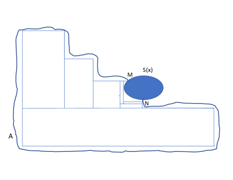
Figure 3. The set $A$ is decomposed into several smaller cubes. The curve $MN$ belongs to $\mathcal{S}(x)$ but not $A$. The cubes cover $A$ but never intersect $\mathcal{S}(x)$. This is similar to the way how meshes are generated in the theory of finite element methods (see [58]).

The next step is to show that (63), (64) and (65) also hold true when $A$ is an open set of $\mathbb{T}^{3}$. Since $A$ is open, there exists a family of rectangles $\{Q_{n}\}_{n=1}^{\infty}$ such that $A=\bigcup_{n=1}^{\infty}Q_{n}$, and the intersection of any two rectangles $Q_{m}$ and $Q_{n}$ in the family is always of measure $0$ (see Figure 1). Using (63)-(65), we arrive at

$$\int_{\mathbb{R}}\int_{\mathbb{T}^{3}}e^{it(\omega(x)-\omega(x-y)-\omega(y))}\chi_{\bigcup_{n=1}^{N}Q_{n}}(y)\mathrm{d}y\mathrm{d}t\geq 0,$$

$$\int_{\mathbb{R}}\int_{\mathbb{T}^{3}}e^{it(\omega(y)-\omega(y-x)-\omega(x))}\chi_{\bigcup_{n=1}^{N}Q_{n}}(y)\mathrm{d}y\mathrm{d}t\geq 0,$$

and

$$\int_{\mathbb{R}}\int_{\mathbb{T}^{3}}e^{it(\omega(x+y)-\omega(x)-\omega(y))}\chi_{\bigcup_{n=1}^{N}Q_{n}}(y)\mathrm{d}y\mathrm{d}t\geq 0,$$

for any $N\geq 1$. Repeating the above stationary phase argument gives

$$\left|\int_{\mathbb{T}^{3}}e^{it(\omega(x)-\omega(x-y)-\omega(y))}\chi_{\bigcup_{n=1}^{N}Q_{n}}(y)\mathrm{d}y\right|\lesssim\frac{1}{\langle t\rangle^{\frac{1}{2}}\sqrt{|1+e^{i2\pi x^{1}}||1+e^{i2\pi x^{2}}||1+e^{i2\pi x^{3}}|}},$$

$$\left|\int_{\mathbb{T}^{3}}e^{it(\omega(y)-\omega(y-x)-\omega(x))}\chi_{\bigcup_{n=1}^{N}Q_{n}}(y)\mathrm{d}y\right|\lesssim\frac{1}{\langle t\rangle^{\frac{1}{2}}\sqrt{|1-e^{i2\pi x^{1}}||1-e^{i2\pi x^{2}}||1-e^{i2\pi x^{3}}|}},$$

and

$$\left|\int_{\mathbb{T}^{3}}e^{it(\omega(x+y)-\omega(x)-\omega(y))}\chi_{\bigcup_{n=1}^{N}Q_{n}}(y)\mathrm{d}y\right|\lesssim\frac{1}{\langle t\rangle^{\frac{1}{2}}\sqrt{|1-e^{i2\pi x^{1}}||1-e^{i2\pi x^{2}}||1-e^{i2\pi x^{3}}|}},$$

with the notice that the constants on the right hand side of the above inequalities are independent of $N$, since $\bigcup_{n=1}^{N}Q_{n}$ is always a subset of $\mathbb{T}^{3}$. By the Lesbesgue dominated convergence theorem, the following inequalities hold true

$$\left|\int_{\mathbb{T}^{3}}e^{it(\omega(x)-\omega(x-y)-\omega(y))}\chi_{A}(y)\mathrm{d}y\right|\lesssim\frac{1}{\langle t\rangle^{\frac{1}{2}}\sqrt{|1+e^{i2\pi x^{1}}||1+e^{i2\pi x^{2}}||1+e^{i2\pi x^{3}}|}},$$ (86)

$$\left|\int_{\mathbb{T}^{3}}e^{it(\omega(y)-\omega(y-x)-\omega(x))}\chi_{A}(y)\mathrm{d}y\right|\lesssim\frac{1}{\langle t\rangle^{\frac{1}{2}}\sqrt{|1-e^{i2\pi x^{1}}||1-e^{i2\pi x^{2}}||1-e^{i2\pi x^{3}}|}},$$ (87)

and

$$\left|\int_{\mathbb{T}^{3}}e^{it(\omega(x+y)-\omega(x)-\omega(y))}\chi_{A}(y)\mathrm{d}y\right|\lesssim\frac{1}{\langle t\rangle^{\frac{1}{2}}\sqrt{|1-e^{i2\pi x^{1}}||1-e^{i2\pi x^{2}}||1-e^{i2\pi x^{3}}|}},$$ (88)

where the constants on the right hand side of (86), (87) and (88) are independent of $A$. In addition, the three index functionals of $A$ are also positive

$$\int_{\mathbb{R}}\int_{\mathbb{T}^{3}}e^{it(\omega(x)-\omega(x-y)-\omega(y))}\chi_{A}(y)\mathrm{d}y\mathrm{d}t\geq 0,$$ (89)

$$\int_{\mathbb{R}}\int_{\mathbb{T}^{3}}e^{it(\omega(y)-\omega(y-x)-\omega(x))}\chi_{A}(y)\mathrm{d}y\mathrm{d}t\geq 0,$$ (90)

and

$$\int_{\mathbb{R}}\int_{\mathbb{T}^{3}}e^{it(\omega(x+y)-\omega(x)-\omega(y))}\chi_{A}(y)\mathrm{d}y\mathrm{d}t\geq 0.$$ (91)

Now, we need to show that (86)-(91) also hold true when $A$ is a Lebesgue measure subset of $\mathbb{T}^{3}$. Since $A$ is Lebesgue measurable, there exists a family $\{A_{n}\}_{n=1}^{\infty}$ of open subsets of $\mathbb{T}^{3}$ such that $A=\bigcap_{n=1}^{\infty}A_{n}$. Note that (86)-(91) can be applied for all $A_{n}$, the Lebesgue dominated convergence theorem also implies that (86)-(91) are indeed true for $A$.

(iii) Countable additivity. The countable additivity is a consequence of the six properties (86)-(91) and the Lebesgue dominate convergence theorem.

(iv) Uniquely defined. In order to prove (iii), we only need to show that for any measurable subset $A$ of $\mathbb{T}^{3}$ and $A\cap\mathcal{S}(x)=\emptyset$, the following identities all hold true

$$\int_{\mathbb{R}}\int_{\mathbb{T}^{3}}e^{it(\omega(x)-\omega(x-y)-\omega(y))}\chi_{A}(y)\mathrm{d}y\mathrm{d}t=0,$$ (92)

$$\int_{\mathbb{R}}\int_{\mathbb{T}^{3}}e^{it(\omega(y)-\omega(y-x)-\omega(x))}\chi_{A}(y)\mathrm{d}y\mathrm{d}t=0,$$ (93)

and

$$\int_{\mathbb{R}}\int_{\mathbb{T}^{3}}e^{it(\omega(x+y)-\omega(x)-\omega(y))}\chi_{A}(y)\mathrm{d}y\mathrm{d}t=0.$$ (94)

Similarly as in Step (ii), we first consider the case where $A$ is a rectangle, $A=I_{1}\times I_{2}\times I_{3}=[a_{1},b_{1}]\times[a_{2},b_{2}]\times[a_{3},b_{3}]$ with $I_{1},I_{2},I_{3}$ being closed intervals of $\mathbb{T}$.

Recall from Proposition 8 that $\mathcal{S}^{1}_{b}(x)$ is the closed set of all wave vectors $y$, such that $x$ is connected to $y$ by a backward collision. Since $A\cap\mathcal{S}(x)=\emptyset$, it is straightforward that $A\cap\mathcal{S}^{1}_{b}(x)=\emptyset$. Since both $A$ and $\mathcal{S}^{1}_{b}(x)$ are both closed set in $\mathbb{T}^{3}$, there exists a constant $\delta>0$ such that for any two wave vectors $z\in A$ and $y\in\mathcal{S}^{1}_{b}(x)$, the distance between $z$ and $y$ always satisfies $|z-y|>\delta>0$. This implies the existence of a constant $\theta>0$ such that

$$|\omega(x)-\omega(z)-\omega(x-z)|>\theta>0$$ (95)

for all $z$ in $A$.

Combining (95) with the approximation (66) used in Step (ii), we find

$$\int_{\mathbb{R}}\int_{\mathbb{T}^{3}}e^{it(\omega(x)-\omega(x-z)-\omega(z))-\epsilon^{2}t^{2}}\chi_{A}(z)\mathrm{d}y\mathrm{d}t\ = \ \frac{C}{\epsilon}\int_{\mathbb{T}^{3}}e^{-\frac{\pi(\omega(x)-\omega(x-z)-\omega(z))^{2}}{\epsilon^{2}}}\chi_{A}(z)\mathrm{d}z$$

$$\ \lesssim \ \frac{1}{\epsilon}\int_{\mathbb{T}^{3}}e^{-\frac{\pi\theta^{2}}{\epsilon^{2}}}\chi_{A}(z)\mathrm{d}z.$$

Using the fact that $A$ is a subset of $\mathbb{T}^{3}$, we deduce

$$\int_{\mathbb{R}}\int_{\mathbb{T}^{3}}e^{it(\omega(x)-\omega(x-z)-\omega(z))-\epsilon^{2}t^{2}}\chi_{A}(z)\mathrm{d}z\mathrm{d}t\ \lesssim \ \frac{e^{-\frac{\pi\theta^{2}}{\epsilon^{2}}}}{\epsilon}\to 0\mbox{ as }\epsilon\to 0.$$ (96)

Again, the same stationary phase argument used in Step 1 can be applied to show that

$$\int_{\mathbb{R}}\int_{\mathbb{T}^{3}}e^{it(\omega(x)-\omega(x-z)-\omega(z))}\chi_{A}(z)\mathrm{d}z\mathrm{d}t=\lim_{\epsilon\to 0}\int_{\mathbb{R}}\int_{\mathbb{T}^{3}}e^{it(\omega(x)-\omega(x-z)-\omega(z))-\epsilon^{2}t^{2}}\chi_{A}(z)\mathrm{d}z\mathrm{d}t=0.$$ (97)

Identity (92) is therefore proved for the case where $A$ is a rectangle and (93), (94) can also be proved by the same argument.

The general case, when $A$ is a measurable set, can be done by the same argument used in Step (ii).

(iv) Boundedness. Applying (86)-(88) to $A=\mathcal{S}(x)$, we obtain that the boundedness of $\mu_{1}(\mathcal{S}(x))$, $\mu_{2}(\mathcal{S}(x))$ and $\mu_{3}(\mathcal{S}(x))$. ∎

Corollary 13.

Given any function $f\in\mathbb{L}^{1}(\mathbb{T}^{3})$ and a collisional invariant region $\mathcal{S}(x)$. Define restriction of $f$ on $\mathcal{S}(x)$ as follows

$$f_{|_{\mathcal{S}(x)}}(y)\ =\ f(y)\mbox{ if }y\in\mathcal{S}(x)\mbox{ and }f_{|_{\mathcal{S}(x)}}(y)\ =\ 0\mbox{ if }y\in\mathbb{T}^{3}\backslash\mathcal{S}(x).$$ (98)

Then

$$\int_{\mathbb{T}^{3}}\delta(\omega(x)-\omega(x-y)-\omega(y))f(y)\mathrm{d}y\ =\ \int_{\mathbb{T}^{3}}\delta(\omega(x)-\omega(x-y)-\omega(y))f_{|_{\mathcal{S}(x)}}(y)\mathrm{d}y,$$ (99)

$$\int_{\mathbb{T}^{3}}\delta(\omega(y)-\omega(y-x)-\omega(x))f(y)\mathrm{d}y\ =\ \int_{\mathbb{T}^{3}}\delta(\omega(y)-\omega(y-x)-\omega(x))f_{|_{\mathcal{S}(x)}}(y)\mathrm{d}y,$$ (100)

and

$$\int_{\mathbb{T}^{3}}\delta(\omega(x+y)-\omega(x)-\omega(y))f(y)\mathrm{d}y\ =\ \int_{\mathbb{T}^{3}}\delta(\omega(x+y)-\omega(x)-\omega(y))f_{|_{\mathcal{S}(x)}}(y)\mathrm{d}y.$$ (101)

Proof.

The proof follows from Proposition 12, Corollary 9 and the fact that $f$ can be approximated by measurable step functions. ∎

Corollary 14.

The edges, i.e. the set $\mathbb{T}^{3}\backslash\mathfrak{S}$ of all wave vectors $y=(y^{1},y^{2},y^{3})$ in which there is an index $i\in\{1,2,3\}$ such that $y^{i}=\pm\frac{1}{2}$ or $0$, is a subset of the no-collision region $\mathfrak{I}$.

Proof.

The corollary follows directly from the proof of Proposition 12. ∎

4.1.3. Lipschitz continuity of set index functionals

In this subsection, we will prove the interesting property that the index functionals of $\mathbb{T}^{3}$, $\mu_{1}(\mathbb{T}^{3})(x)$, $\mu_{2}(\mathbb{T}^{3})(x)$ and $\mu_{3}(\mathbb{T}^{3})(x)$, are Lipschitz continuous functions, if for all $i=1,2,3$, $x^{i}\neq\pm\frac{1}{2},0$ with $x=(x^{1},x^{2},x^{3})$. For the sake of simplicity, in this section, we denote $\mu_{1}(\mathbb{T}^{3})$, $\mu_{2}(\mathbb{T}^{3})$ and $\mu_{3}(\mathbb{T}^{3})$ by $F(x)$, $G(x)$ and $H(x)$.

Proposition 15.

The functions $F(x)$, $G(x)$ and $H(x)$ are Lipchitz continuous on $\mathbb{T}^{3}$ excluding the edges, i.e. the set $\mathfrak{S}$ of all points $x=(x^{1},x^{2},x^{3})$ in which $x^{i}\neq\pm\frac{1}{2},0$, for all $i=1,2,3$.

Proof.

First, we prove that $F$ is continuous functions on $\mathfrak{S}$. Let $x$ be a point in $\mathfrak{S}$ and a sequence $\{x_{n}\}_{n=1}^{\infty}\subset\mathfrak{S}$ such that $\lim_{n\to\infty}x_{n}=x$. Since the set $\mathbb{T}^{3}\backslash\mathfrak{S}$ is closed, without loss of generality, we suppose that there exists a ball $B(x,r)$ with radius $r$ and centered at $x$ such that $B(x,r)\cap(\mathbb{T}^{3}\backslash\mathfrak{S})=\emptyset$ and then $\{x_{n}\}_{n=1}^{\infty}\subset B(x,r)$. From the proof of Proposition 12 and the assumption $B(x,r)\cap(\mathbb{T}^{3}\backslash\mathfrak{S})=\emptyset$, it follows

$$\left|\int_{\mathbb{T}^{3}}e^{it(\omega(x)-\omega(x-y)-\omega(y))}\mathrm{d}y\right|\ \lesssim \ \frac{1}{\langle t\rangle^{\frac{3}{2}}\sqrt{|1+e^{2\pi x^{1}}||1+e^{2\pi x^{2}}||1+e^{2\pi x^{3}}|}}\ \lesssim\ 1.$$ (102)

By the Lebesgue dominated convergence theorem, $\lim_{n\to\infty}F(x_{n})=F(x)$ and the function $F$ is then continuous on $\mathfrak{S}$. Let $x,z$ be two elements of $\mathfrak{S}$ and suppose that there exists a number $r>0$ such that $z\in B(x,r)$, $x\in B(z,r)$ and $B(x,r),B(z,r)\cap(\mathbb{T}^{3}\backslash\mathfrak{S})=\emptyset$. We compute the different between $F(x)$ and $F(z)$, using the mean value theorem

$$F(x)-F(z)\ = \ i|x-z|\int_{0}^{1}\int_{\mathbb{R}}\int_{\mathbb{T}^{3}}e^{it(\omega(sx+(1-s)z)-\omega(sx+(1-s)z-y)-\omega(y))}\times$$ (103)

$$\indent\ \times\left[\frac{x^{1}-z^{1}}{|x-z|}(\sin(sx^{1}+(1-s)z^{2})-\sin(sx^{1}+(1-s)z^{1}-y^{1}))-\right.$$

$$\indent\ +\left.\frac{x^{2}-z^{2}}{|x-z|}(\sin(sx^{2}+(1-s)z^{2})-\sin(sx^{2}+(1-s)z^{2}-y^{2}))+\right.$$

$$\indent\ +\left.\frac{x^{3}-z^{3}}{|x-z|}(\sin(sx^{3}+(1-s)z^{3})-\sin(sx^{3}+(1-s)z^{3}-y^{3}))\right]\mathrm{d}y\mathrm{d}t\mathrm{d}s.$$

Again, the stationary phase method, used in the proof of Proposition 12, yields

$$\ \left|i|x-z|\int_{\mathbb{T}^{3}}e^{it(\omega(sx+(1-s)z)-\omega(sx+(1-s)z-y)-\omega(y))}\times\right.$$ (104)

$$\indent\ \times\left[\frac{x^{1}-z^{1}}{|x-z|}(\sin(sx^{1}+(1-s)z^{1})-\sin(sx^{1}+(1-s)z^{1}-y^{1}))-\right.$$

$$\indent\ +\left.\frac{x^{2}-z^{2}}{|x-z|}(\sin(sx^{2}+(1-s)z^{2})-\sin(sx^{2}+(1-s)z^{2}-y^{2}))+\right.$$

$$\indent\ +\left.\left.\frac{x^{3}-z^{3}}{|x-z|}(\sin(sx^{3}+(1-s)z^{3})-\sin(sx^{3}+(1-s)z^{3}-y^{3}))\right]\mathrm{d}y\right|$$

$$\lesssim \ \frac{1}{\langle t\rangle^{\frac{3}{2}}\sqrt{|1+e^{2\pi(sx^{1}+(1-s)z^{1})}||1+e^{2\pi(sx^{2}+(1-s)z^{2})}||1+e^{2\pi(sx^{3}+(1-s)z^{3})}|}},$$

which, after integrating in $s$ and $t$ and plugging back to (103), leads to

$$|F(x)-F(z)|\ \lesssim$$ (105)

$$\ \lesssim \ |x-z|\int_{0}^{1}\int_{\mathbb{R}}\frac{\mathrm{d}t\mathrm{d}s}{\langle t\rangle^{\frac{3}{2}}\sqrt{|1+e^{2\pi(sx^{1}+(1-s)z^{1})}||1+e^{2\pi(sx^{2}+(1-s)z^{2})}||1+e^{2\pi(sx^{3}+(1-s)z^{3})}|}}.$$

Integrating in $t$

$$|F(x)-F(z)|\ \lesssim \ |x-z|\int_{0}^{1}\frac{\mathrm{d}s}{\sqrt{|1+e^{2\pi(sx^{1}+(1-s)z^{1})}||1+e^{2\pi(sx^{2}+(1-s)z^{2})}||1+e^{2\pi(sx^{3}+(1-s)z^{3})}|}},$$ (106)

which, by the fact that $z\in B(x,r)$, $x\in B(z,r)$ and $B(x,r),B(z,r)\cap(\mathbb{T}^{3}\backslash\mathfrak{S})=\emptyset$, yields $|F(x)-F(z)|\ \lesssim\ |x-z|$. Therefore the function $F$ is Lipschitz on $\mathfrak{S}$. By the same argument, $G,H$ are also Lipschitz continuous. ∎

4.1.4. Weak formulation, local conservation of momentum and energy on collisional invariant regions

Lemma 16.

For any smooth function $f(k)$, there holds

$$\int_{\mathbb{T}^{3}}Q_{c}[f](k)\varphi(k)\mathrm{d}k = \iiint_{\mathbb{T}^{9}}[\omega\omega_{1}\omega_{2}]^{-1}\delta(k-k_{1}-k_{2})\delta(\omega-\omega_{1}-\omega_{2})\times$$

$$\times[f_{1}f_{2}-ff_{1}-ff_{2}]\Big{(}\varphi(k)-\varphi(k_{1})-\varphi(k_{2})\Big{)}\;\mathrm{d}k\mathrm{d}k_{1}\mathrm{d}k_{2}$$

for any smooth test function $\varphi$.

If $\varphi$ is supported in a collisional invariant region $\mathcal{S}(x)$, then, we also have

$$\int_{\mathbb{T}^{3}}Q_{c}[f](k)\varphi(k)\mathrm{d}k = \iiint_{\mathcal{S}(x)\times\mathcal{S}(x)\times\mathcal{S}(x)}[\omega\omega_{1}\omega_{2}]^{-1}\delta(k-k_{1}-k_{2})\delta(\omega-\omega_{1}-\omega_{2})\times$$

$$\times[f_{1}f_{2}-ff_{1}-ff_{2}]\Big{(}\varphi(k)-\varphi(k_{1})-\varphi(k_{2})\Big{)}\;\mathrm{d}k\mathrm{d}k_{1}\mathrm{d}k_{2}.$$

Proof.

We have

$$\ \int_{\mathbb{T}^{3}}Q[f](k)\varphi(k)\mathrm{d}k\ =$$

$$=\ \int_{\mathbb{T}^{9}}[\omega\omega_{1}\omega_{2}]^{-1}\delta(k-k_{1}-k_{2})\delta(\omega-\omega_{1}-\omega_{2})[f_{1}f_{2}-ff_{1}-ff_{2}]\varphi(k)\mathrm{d}k\mathrm{d}k_{1}\mathrm{d}k_{2}$$

$$-\ \int_{\mathbb{T}^{9}}[\omega\omega_{1}\omega_{2}]^{-1}\delta(k_{1}-k-k_{2})\delta(\omega_{1}-\omega-\omega_{2})[f_{2}f-ff_{1}-f_{1}f_{2}]\varphi(k)\mathrm{d}k\mathrm{d}k_{1}\mathrm{d}k_{2}$$

$$-\ \int_{\mathbb{T}^{9}}[\omega\omega_{1}\omega_{2}]^{-1}\delta(k_{1}-k-k_{2})\delta(\omega_{1}-\omega-\omega_{2})[f_{2}f-ff_{1}-f_{1}f_{2}]\varphi(k)\mathrm{d}k\mathrm{d}k_{1}\mathrm{d}k_{2},$$

by switching the variables $k\leftrightarrow k_{1}$ and $k\leftrightarrow k_{2}$ in the second and third integrals, respectively, the first identity follows. The second identity follows straightforwardly from Corollary 13 and the first identity. ∎

As a consequence, we obtain the following corollary.

Corollary 17 (Conservation of momentum and energy on collisional invariant regions).

Smooth solutions $f(t,k)$ of (2), with initial data $f(0,k)=f_{0}(k)$, satisfy

$$\int_{\mathcal{S}(x)}f(t,k)k\mathrm{d}k = \int_{\mathcal{S}(x)}f_{0}(k)k\mathrm{d}k.$$ (107)

$$\int_{\mathcal{S}(x)}f(t,k)\omega(k)\mathrm{d}k = \int_{\mathcal{S}(x)}f_{0}(k)\omega(k)\mathrm{d}k.$$ (108)

for all $t\geq 0$ and for all $x\in\mathfrak{V}$, defined in Proposition 6.

Proof.

This follows from Lemma 16 by taking $\varphi(k)=k^{1},k^{2},k^{3}$ and $\omega(k)$ with $k=(k^{1},k^{2},k^{3})$. ∎

4.1.5. Local equilibria on collisional invariant regions

In this section, we establish the form of local equilibria on collisional invariant regions. The key different between these local equilibria and the equilibria of classical kinetic equations is that these equilibria are only defined locally on collisional invariant regions. This is a very special feature of the 3-wave kinetic equation.

Lemma 18 ($C^{2}$-collisional invariants).

Let $\psi\in C^{2}(\mathcal{S}(x))$ be a collisional invariant on the collisional invariant region $\mathcal{S}(x)$, in the following sense. For any wave vectors $k,k_{1},k_{2}\in\mathcal{S}(x)$,

$$k=k_{1}+k_{2},\ \ \ \ \omega(k)=\omega(k_{1})+\omega(k_{2}),$$

we have

$$\psi(k)=\psi(k_{1})+\psi(k_{2}).$$

Then there exist a constant $a_{x}\in\mathbb{R}$ and a vector $b_{x}\in\mathbb{R}^{3}$, such that

$$\psi(k)=a_{x}\omega(k)+b_{x}\cdot k.$$

Proof.

Let us first prove that for $k\in\mathcal{S}(x)$, the partial derivatives $\partial_{k^{j}}\psi(k)$, with $k=(k^{1},k^{2},k^{3})$, are well-defined. Without loss of generality, we only prove that the partial derivative with respect to the first component $\partial_{k^{1}}\psi(k)$ is well-defined. Since $k\in\mathcal{S}(x)$, there are two wave vectors $k_{1},k_{2}$ such that either $k=k_{1}+k_{2}$ and $\omega(k)=\omega(k_{1})+\omega(k_{2})$; or $k+k_{1}=k_{2}$ and $\omega(k)+\omega(k_{1})=\omega(k_{2})$.

Case 1: $k=k_{1}+k_{2}$ and $\omega(k)=\omega(k_{1})+\omega(k_{2})$. Since $\psi\in C^{2}(\mathbb{T}^{3})$, in order to show that $\partial_{k^{1}}\psi(k)$ is well-defined at $k^{1}\in\mathbb{T}$, we only have to prove that there exists $\epsilon>0$ such that for each $\bar{k}^{1}\in(k^{1}-\epsilon,k^{1}+\epsilon)$ there are $\bar{k}^{2},\bar{k}^{3}\in\mathbb{T}^{3}$, $\bar{k}=(\bar{k}^{1},\bar{k}^{2},\bar{k}^{3})\in\mathcal{S}(x)$. For any $x,y\in\mathbb{T}$, define

$$F(x,y)=\cos(2\pi(x+y))-\cos(2\pi x)-\cos(2\pi y).$$

Since $k=(k^{1},k^{2},k^{3})=k_{1}+k_{2}=(k^{1}_{1},k^{2}_{1},k^{3}_{1})+(k^{1}_{2},k^{2}_{2},k^{3}_{2})$, we then have

$$F(k_{1}^{1},k_{2}^{1})+F(k_{1}^{2},k_{2}^{2})+F(k_{1}^{3},k_{2}^{3})=-\omega_{0}/2-3.$$

Now, we develop

$$\begin{aligned} F(x,y)+1\ =&\ -\cos(2\pi x)-\cos(2\pi y)+1+\cos(2\pi(x+y))\\ =&\ 2\cos\left(\pi({x+y})\right)\left[-\cos\left(\pi({x-y})\right)+\cos\left(\pi({x+y})\right)\right]\\ =&\ -4\cos\left(\pi({x+y})\right)\sin\left(\pi x\right)\sin\left(\pi y\right)\ \leq 4.\end{aligned}.$$

Hence $\max_{x,y\in\mathbb{T}}F(x,y)=3$ when $(x,y)=\left(\frac{1}{2},-\frac{1}{2}\right)=\left(-\frac{1}{2},\frac{1}{2}\right).$ We observe that the sum $F(k_{1}^{2},k_{2}^{2})+F(k_{1}^{3},k_{2}^{3})$ must be strictly smaller than $6$; otherwise, $F(k_{1}^{1},k_{2}^{1})=-\omega_{0}/2-9<-9$, which is a contradiction.

Since $F(k_{1}^{2},k_{2}^{2})+F(k_{1}^{3},k_{2}^{3})<6$, then for any $\delta$ small, either positive or negative, there exist $\delta_{1},\delta_{2}$, either positive or negative, such that

$$F(k_{1}^{1}+\delta,k_{2}^{1})+F(k_{1}^{2}+\delta_{1},k_{2}^{2})+F(k_{1}^{3}+\delta_{2},k_{2}^{3})=-\omega_{0}/2-3,$$

due to the continuity of $F$. If $\bar{k}^{1}=k^{1}+\delta$, then we choose $\bar{k}^{2}=k^{1}+\delta_{1}$ and $\bar{k}^{3}=k^{3}+\delta_{2}$.

Case 2: $k+k_{1}=k_{2}$ and $\omega(k)+\omega(k_{1})=\omega(k_{2})$. Similar as Case 1, we only need to show that, for each $k^{1}\in\mathbb{T}$, there exists $\epsilon>0$ such that for each $\bar{k}^{1}\in(k^{1}-\epsilon,k^{1}+\epsilon)$ there are $\bar{k}^{2},\bar{k}^{3}\in\mathbb{T}^{3}$, $\bar{k}=(\bar{k}^{1},\bar{k}^{2},\bar{k}^{3})\in\mathcal{S}(x)$. Since $k_{2}=(k_{2}^{1},k_{2}^{2},k_{2}^{3})=k_{1}+k=(k^{1}_{1},k^{2}_{1},k^{3}_{1})+(k^{1},k^{2},k^{3})$, we then have

$$F(k_{1}^{1},k^{1})+F(k_{1}^{2},k^{2})+F(k_{1}^{3},k^{3})=-\omega_{0}/2-3.$$

Since $F(k_{1}^{2},k^{2})+F(k_{1}^{3},k^{3})<6$, then for any $\delta$ small, either positive or negative, there exist $\delta_{1},\delta_{2}$, either positive or negative, such that

$$F(k_{1}^{1},k^{1}+\delta)+F(k_{1}^{2},k^{2}+\delta_{1})+F(k_{1}^{3},k^{3}+\delta_{2})=-\omega_{0}/2-3,$$

due to the continuity of $F$. If $\bar{k}^{1}=k^{1}+\delta$, then we choose $\bar{k}^{2}=k^{1}+\delta_{1}$ and $\bar{k}^{3}=k^{3}+\delta_{2}$.

Since on $\mathcal{S}(x)$, $\psi(k)$ is a function of $\omega(k)$ and $k$, there exists a twice differentiable continuous function $\phi\in C^{2}(\mathbb{R}_{+}\times\mathbb{T}^{3})$ such that $\psi(k)=\varphi(\omega(k),k)$.

For $k\in\mathcal{S}(x)$, there exist two wave vectors $k_{1},k_{2}\in\mathbb{T}^{3}$, such that either $k=k_{1}+k_{2}$ and $\omega(k)=\omega(k_{1})+\omega(k_{2})$, or $k+k_{1}=k_{2}$ and $\omega(k)+\omega(k_{1})=\omega(k_{2})$. We assume that $k=k_{1}+k_{2}$ and $\omega(k)=\omega(k_{1})+\omega(k_{2})$, $k_{1},k_{2}\in\mathbb{T}^{3}$, the other case can be consider with exactly the same argument. As we observe before, $k_{1},k_{2}$ also belong to $\mathcal{S}(x)$ due to the fact that $k$ is connected to both $k_{1},k_{2}$ by one-collisions. We have

$$\psi(k_{1})+\psi(k_{2})=\psi(k)=\varphi(\omega(k),k)=\varphi(\omega(k_{1})+\omega(k_{2}),k_{1}+k_{2}).$$

Differentiating the above identity with respect to $k^{j}_{1}$ and $k^{j}_{2}$ yields

$$\partial_{k^{j}_{1}}\psi(k_{1})\ = \ \partial_{r}\varphi(\omega(k),k)\partial_{k^{j}_{1}}\omega(k_{1})+\partial_{k^{j}_{1}}\varphi(\omega(k),k),$$

$$\partial_{k^{j}_{2}}\psi(k_{2})\ = \ \partial_{r}\varphi(\omega(k),k)\partial_{k^{j}_{2}}\omega(k_{2})+\partial_{k^{j}_{2}}\varphi(\omega(k),k).$$

Letting $i\in\{1,2,3\}$ be a different index, we manipulate the above identity as

$$\ (\partial_{k^{j}_{1}}\psi(k_{1})-\partial_{k^{j}_{2}}\psi(k_{2}))(\partial_{k^{i}_{1}}\omega(k_{1})-\partial_{k^{i}_{2}}\omega(k_{2}))$$

$$\ = \ (\partial_{k^{i}_{1}}\psi(k_{1})-\partial_{k^{i}_{2}}\psi(k_{2}))(\partial_{k^{j}_{1}}\omega(k_{1})-\partial_{k^{j}_{2}}\omega(k_{2})).$$

We differentiate the above identity in $k_{1}$, with $l$ being an index in $\{1,2,3\}$

$$\ \partial_{k^{j}_{1}}\partial_{k^{l}_{1}}\psi(k_{1})(\partial_{k^{i}_{1}}\omega(k_{1})-\partial_{k^{i}_{2}}\omega(k_{2}))+(\partial_{k^{j}_{1}}\psi(k_{1})-\partial_{k^{j}_{2}}\psi(k_{2}))\partial_{k^{i}_{1}}\partial_{k^{l}_{1}}\omega(k_{1})$$

$$\ = \ \partial_{k^{i}_{1}}\partial_{k^{l}_{1}}\psi(k_{1})(\partial_{k^{j}_{1}}\omega(k_{1})-\partial_{k^{j}_{2}}\omega(k_{2}))+(\partial_{k^{i}_{1}}\psi(k_{1})-\partial_{k^{i}_{2}}\psi(k_{2}))\partial_{k^{j}_{1}}\partial_{k^{l}_{1}}\omega(k_{1}),$$

and now in $k_{2}$, with $h$ being an index in $\{1,2,3\}$

$$\ \partial_{k^{j}_{1}}\partial_{k^{l}_{1}}\psi(k_{1})\partial_{k^{i}_{2}}\partial_{k^{h}_{2}}\omega(k_{2})+\partial_{k^{j}_{2}}\partial_{k^{h}_{2}}\psi(k_{2})\partial_{k^{i}_{1}}\partial_{k^{l}_{1}}\omega(k_{1})$$

$$\ = \ \partial_{k^{i}_{1}}\partial_{k^{l}_{1}}\psi(k_{1})\partial_{k^{j}_{2}}\partial_{k^{h}_{2}}\omega(k_{2})+\partial_{k^{i}_{2}}\partial_{k^{h}_{2}}\psi(k_{2})\partial_{k^{j}_{1}}\partial_{k^{l}_{1}}\omega(k_{1}).$$

A particular case of the above identity is the following

$$\ \partial_{k^{i}_{1}}^{2}\psi(k_{1})\partial_{k^{j}_{2}}^{2}\omega(k_{2})\ =\ \partial_{k^{j}_{1}}^{2}\psi(k_{1})\partial_{k^{i}_{2}}^{2}\omega(k_{2}),$$

which implies

$$\partial_{k^{i}_{1}}^{2}\psi(k_{1})\cos(k_{2}^{j})\ =\ \partial_{k^{i}_{2}}^{2}\psi(k_{1})\cos(k_{1}^{j}),$$

for any $k_{1},k_{3}\in\mathcal{S}(x)$, and $k_{1},k_{2}$ are connected to $k_{1}+k_{2}$ by one collision.

Hence $\psi(k)=a_{x}\omega(k)+b_{x}\cdot k+c_{x}$, with $a_{x},c_{x}\in\mathbb{R}$, $b_{x}\in\mathbb{R}^{3}$ for any $k\in\mathcal{S}(x)$. By the fact $\psi(k)=\psi(k_{1})+\psi(k_{2})$ whenever $k$ is connected to $k_{1},k_{2}$ by one-collisions, it is straightforward that $c_{x}=0$. ∎

Proposition 19 ($L^{1}$-collisional invariants).

Let $\psi\in L^{1}(\mathcal{S}(x))$ be a collisional invariant on the collisional invariant region $\mathcal{S}(x)$, in the following sense. For any $k\in\mathcal{S}(x)$, such that

$$k=k_{1}+k_{2},\ \ \ \ \omega(k)=\omega(k_{1})+\omega(k_{2}),$$

we have

$$\psi(k)=\psi(k_{1})+\psi(k_{2}).$$

Then there exist a constant $a_{x}\in\mathbb{R}$ and a vector $b_{x}\in\mathbb{R}^{3}$, such that

$$\psi(k)=a_{x}\omega(k)+b_{x}\cdot k.$$

Proof.

For any function $\phi\in C^{\infty}(\mathbb{T}^{3})$, we define the standard mollifier $\phi_{\delta}(k)=\delta^{-3}\phi\left(\frac{k}{\delta}\right)$ and the standard approximation $\psi_{\delta}=\psi*\phi_{\delta}$ with $\delta>0$. It is then classical that $\lim_{\delta\to 0}\|\psi_{\delta}-\psi\|_{L^{1}(\mathcal{S}(x))}=0.$

Since $\psi(k)=\psi(k_{1})+\psi(k_{2})$, we also have $\psi_{\delta}(k)=\psi_{\delta}(k_{1})+\psi_{\delta}(k_{2})$. Lemma 18 can be applied to $\psi_{\delta}$, yielding $\psi_{\delta}(k)=a_{x}^{\delta}\omega(k)+b_{x}^{\delta}\cdot k$ for some constant $a_{x}^{\delta}\in\mathbb{R}$ and vector $b_{x}^{\delta}\in\mathbb{R}^{3}$. The conclusion of the Proposition then follows after passing $\delta$ to $0$, while taking into account the limit $\lim_{\delta\to 0}\|\psi_{\delta}-\psi\|_{L^{1}(\mathcal{S}(x))}=0.$ ∎

Proposition 20 (Equilibria in Collisional Invariant Regions).

Given a collisional invariant region $\mathcal{S}(x)$, a function $\mathcal{F}^{c}(k)\in C(\mathcal{S}(x))$ is said to be a local equilibrium of $Q_{c}$ on $\mathcal{S}(x)$ if and only if $Q_{c}[\mathcal{F}^{c}](k)=0$ and $\mathcal{F}^{c}(k)>0$ for all $k\in\mathcal{S}(x)$.

Let $(M_{x},E_{x})\in\mathbb{R}^{3}\times\mathbb{R}_{+}$ be a pair of admissible constants in the sense of Definition 1 and assume further the system of 4 equations with 4 variables $(a_{x},b_{x})=(a_{x},b_{x}^{1},b_{x}^{2},b_{x}^{3})\in\mathbb{R}_{+}\times\mathbb{R}^{3}$

$$\int_{\mathcal{S}(x)}\frac{\omega(k)}{a_{x}\omega(k)+b_{x}\cdot k}\mathrm{d}k\ = \ E_{x},$$ (109)

$$\int_{\mathcal{S}(x)}\frac{k}{a_{x}\omega(k)+b_{x}\cdot k}\mathrm{d}k\ = \ M_{x},$$

has a unique solution $a_{x}\in\mathbb{R}_{+}$ and $b_{x}\in\mathbb{R}^{3}$ such that $a_{x}\omega(k)+b_{x}\cdot k>0$ for all $k\in\mathcal{S}(x)$; the local equilibrium on $\mathcal{S}(x)$ of $Q_{c}$ can be uniquely determined as

$$\mathcal{F}^{c}(k)\ =\ \frac{1}{a_{x}\omega(k)+b_{x}\cdot k},$$ (110)

subjected to the local energy and local moment constraints

$$\int_{\mathcal{S}(x)}\mathcal{F}^{c}(k)\omega(k)\mathrm{d}k\ = \ E_{x},$$ (111)

$$\int_{\mathcal{S}(x)}\mathcal{F}^{c}(k)k\mathrm{d}k\ = \ M_{x}.$$

Proof.

Since $Q_{c}[\mathcal{F}^{c}](k)=0$ for all $k\in\mathcal{S}(x)$, using $\frac{1}{\mathcal{F}^{c}}$ as a test function, we obtain

$$0\ = \ \int_{\mathcal{S}(x)}Q_{c}[\mathcal{F}^{c}](k)\frac{1}{\mathcal{F}^{c}(k)}\mathrm{d}k$$ (112)

$$\ = \ \int_{\mathcal{S}(x)\times\mathcal{S}(x)\times\mathcal{S}(x)}\delta(k-k_{1}-k_{2})\delta(\omega-\omega_{1}-\omega_{2})[\mathcal{F}^{c}_{1}\mathcal{F}^{c}_{2}-\mathcal{F}^{c}_{1}\mathcal{F}^{c}-\mathcal{F}^{c}_{2}\mathcal{F}^{c}]\times$$

$$\ \times\left[\frac{1}{\mathcal{F}^{c}}-\frac{1}{\mathcal{F}^{c}_{1}}-\frac{1}{\mathcal{F}^{c}_{2}}\right]\mathrm{d}k\mathrm{d}k_{1}\mathrm{d}k_{2}$$

$$\ = \ \int_{\mathcal{S}(x)\times\mathcal{S}(x)\times\mathcal{S}(x)}\delta(k-k_{1}-k_{2})\delta(\omega-\omega_{1}-\omega_{2})\mathcal{F}^{c}\mathcal{F}^{c}_{1}\mathcal{F}^{c}_{2}\left[\frac{1}{\mathcal{F}^{c}}-\frac{1}{\mathcal{F}^{c}_{1}}-\frac{1}{\mathcal{F}^{c}_{2}}\right]^{2}\mathrm{d}k\mathrm{d}k_{1}\mathrm{d}k_{2},$$

which implies $\frac{1}{\mathcal{F}^{c}}-\frac{1}{\mathcal{F}^{c}_{1}}-\frac{1}{\mathcal{F}^{c}_{2}}=0$ for all $k,k_{1},k_{2}\in\mathcal{S}(x)$ satisfying $k=k_{1}+k_{2}$ and $\omega=\omega_{1}+\omega_{2}$. Therefore $\frac{1}{\mathcal{F}^{c}}$ is a collisional invariant; and by Proposition 19, $\mathcal{F}^{c}$ takes the form (110), given that the system of 4 equations and 4 variables (109) has a unique solution $(a_{x},b_{x})$.

∎

4.1.6. Entropy formulation on the collisional invariant region $\mathcal{S}(x)$

Let $f$ be a positive solution of (2), we define the local entropy on the collisional invariant region $\mathcal{S}(x)$ as follows

$$S_{c,\mathcal{S}(x)}[f]\ =\ \int_{\mathcal{S}(x)}s_{c}[f]\mathrm{d}k\ =\ \int_{\mathcal{S}(x)}\ln(f)\mathrm{d}k.$$ (113)

In the sequel, we only consider the local entropy on one collisional invariant region, then, for the sake of simplicity, we denote $S_{c,\mathcal{S}(x)}[f]$ by $S_{c}[f]$.

Now, we take the derivative in time of $S_{c}[f]$

$$\partial_{t}S_{c}[f]\ =\ \int_{\mathcal{S}(x)}\frac{\partial_{t}f}{f}\mathrm{d}k.$$ (114)

Replacing the quantity $\partial_{t}f$ in the above formulation by the right hand side of (2) , we find

$$\ \partial_{t}S_{c}[f]\ = \iiint_{\mathcal{S}(x)\times\mathcal{S}(x)\times\mathcal{S}(x)}[\omega\omega_{1}\omega_{2}]^{-1}\delta(k-k_{1}-k_{2})\delta(\omega-\omega_{1}-\omega_{2})\times$$ (115)

$$\times[f_{1}f_{2}-ff_{1}-ff_{2}]\frac{1}{f}\mathrm{d}k\mathrm{d}k_{1}\mathrm{d}k_{2}$$

$$-\ 2\iiint_{\mathcal{S}(x)\times\mathcal{S}(x)\times\mathcal{S}(x)}[\omega\omega_{1}\omega_{2}]^{-1}\delta(k_{1}-k-k_{2})\delta(\omega_{1}-\omega-\omega_{2})\times$$

$$\times[f_{2}f-ff_{1}-f_{1}f_{2}]\frac{1}{f}\mathrm{d}k\mathrm{d}k_{1}\mathrm{d}k_{2}.$$

We now apply Lemma 16 to the above identity to get

$$\ \partial_{t}S[f]\ = \iiint_{\mathcal{S}(x)\times\mathcal{S}(x)\times\mathcal{S}(x)}[\omega\omega_{1}\omega_{2}]^{-1}\delta(k-k_{1}-k_{2})\delta(\omega-\omega_{1}-\omega_{2})[f_{1}f_{2}-ff_{1}-ff_{2}]\times$$ (116)

$$\times\left[\frac{1}{f_{2}}+\frac{1}{f_{1}}-\frac{1}{f}\right]\mathrm{d}k\mathrm{d}k_{1}\mathrm{d}k_{2}.$$

By noting that

$$f_{1}f_{2}-ff_{1}-ff_{2}=ff_{1}f_{2}\left[\frac{1}{f_{1}}+\frac{1}{f_{2}}-\frac{1}{f}\right],$$

we obtain from (116) the following entropy identity

$$\ \partial_{t}S_{c}[f]\ = \ \int_{\mathcal{S}(x)}[\omega\omega_{1}\omega_{2}]^{-1}\delta(k-k_{1}-k_{2})\delta(\omega-\omega_{1}-\omega_{2})ff_{1}f_{2}\times$$ (117)

$$\times \left[\frac{1}{f_{1}}+\frac{1}{f_{2}}-\frac{1}{f}\right]^{2}\mathrm{d}k\mathrm{d}k_{1}\mathrm{d}k_{2}$$

$$=: \ D_{c}[f].$$

It is clear that the quantity $D_{c}[f]$ is positive. Borrowing the idea of [16, 59], we now define the inverse of $f$

$$g=\frac{1}{f}.$$ (118)

As a consequence, the formula (117) can be expressed in the following form

$$\ \partial_{t}S_{c}[f]\ =\ D_{c}[f]\ =\ \mathbb{D}_{c}[g]\ := \iiint_{\mathcal{S}(x)\times\mathcal{S}(x)\times\mathcal{S}(x)}[\omega\omega_{1}\omega_{2}]^{-1}\delta(k-k_{1}-k_{2})\delta(\omega-\omega_{1}-\omega_{2})\times$$ (119)

$$\times \frac{\left[g_{1}+g_{2}-g\right]^{2}}{gg_{1}g_{2}}\mathrm{d}k\mathrm{d}k_{1}\mathrm{d}k_{2}.$$

4.1.7. Cutting off and splitting the collision operator on the collisional invariant region $\mathcal{S}(x)$

In this subsection, we follow the idea of [16] to introduce a cut-off version for the collision operator $Q_{c}[f]$. The intuition behind this cut-off operator is explained below. We expect that as $t$ tends to infinity, the solution $f$ of (2) converges to an equilibrium, which is a function bounded from above and below by positive constants. Since the equilibrium is bounded from above and below, it is not affected by the cut-off operator. As a result, the solution $f$ is expected to be unchanged, under the effect of the cut-off operator, as $t$ goes to infinity.

Let $\varrho_{N}$ (for $0<N\leq\infty$) be a function in $C^{1}(\mathbb{R}_{+})$ satisfying $\varrho_{N}[z]=1$ when $\frac{1}{N}\leq z\leq N$, $\varrho_{N}[z]=0$ when $0\leq z\leq\frac{1}{2N}$ and $z\geq 2N$, and $0\leq\varrho_{N}[z]\leq 1$ when $\frac{1}{2N}\leq z\leq\frac{1}{N}$ and $N\leq z\leq 2N$. For $f\in C^{1}(\mathcal{S}(x))$ and $0<N\leq\infty$, define the cut-off function

$$\chi_{N}[f]=\varrho_{N}[f]\varrho_{N}[|\nabla f|].$$ (120)

Note that $\chi_{\infty}[f]=1$ for all $f\in C^{1}(\mathcal{S}(x))$.

We set the cut-off collision operator on the collisional invariant region $\mathcal{S}(x)$ for $f$ and for $g$ defined in (118)

$$Q_{c}^{N}[f](k)=$$ (121)

$$=\ \int_{\mathcal{S}(x)\times\mathcal{S}(x)}[\omega\omega_{1}\omega_{2}]^{-1}\chi_{N}^{*}\delta(k-k_{1}-k_{2})\delta(\omega-\omega_{1}-\omega_{2})[f_{1}f_{2}-ff_{1}-ff_{2}]\mathrm{d}k_{1}\mathrm{d}k_{2}$$

$$\indent-\ 2\int_{\mathcal{S}(x)\times\mathcal{S}(x)}[\omega\omega_{1}\omega_{2}]^{-1}\chi_{N}^{*}\delta(k_{1}-k-k_{2})\delta(\omega_{1}-\omega-\omega_{2})[f_{2}f-ff_{1}-f_{1}f_{2}]\mathrm{d}k_{1}\mathrm{d}k_{2}$$

$$=\ \int_{\mathcal{S}(x)\times\mathcal{S}(x)}[\omega\omega_{1}\omega_{2}]^{-1}\chi_{N}^{*}[gg_{1}g_{2}]^{-1}\delta(k-k_{1}-k_{2})\delta(\omega-\omega_{1}-\omega_{2})[g-g_{1}-g_{2}]\mathrm{d}k_{1}\mathrm{d}k_{2}$$

$$\indent-\ 2\int_{\mathcal{S}(x)\times\mathcal{S}(x)}[\omega\omega_{1}\omega_{2}]^{-1}\chi_{N}^{*}[gg_{1}g_{2}]^{-1}\delta(k_{1}-k-k_{2})\delta(\omega_{1}-\omega-\omega_{2})[g_{1}-g_{2}-g]\mathrm{d}k_{1}\mathrm{d}k_{2},$$

in which

$$\chi_{N}^{*}=\chi_{N}[f]\chi_{N}[f_{1}]\chi_{N}[f_{2}]=\chi_{N}[1/g]\chi_{N}[1/g_{1}]\chi_{N}[1/g_{2}].$$ (122)

When $N=\infty$, we have that

$$Q_{c}^{N}[f](k) =Q_{c}^{\infty}[f](k)$$ (123)

$$=\ \int_{\mathcal{S}(x)\times\mathcal{S}(x)}[\omega\omega_{1}\omega_{2}]^{-1}\delta(k-k_{1}-k_{2})\delta(\omega-\omega_{1}-\omega_{2})[f_{1}f_{2}-ff_{1}-ff_{2}]\mathrm{d}k_{1}\mathrm{d}k_{2}$$

$$\indent-\ 2\int_{\mathcal{S}(x)\times\mathcal{S}(x)}[\omega\omega_{1}\omega_{2}]^{-1}\delta(k_{1}-k-k_{2})\delta(\omega_{1}-\omega-\omega_{2})[f_{2}f-ff_{1}-f_{1}f_{2}]\mathrm{d}k_{1}\mathrm{d}k_{2}$$

$$=\ \int_{\mathcal{S}(x)\times\mathcal{S}(x)}[\omega\omega_{1}\omega_{2}]^{-1}[gg_{1}g_{2}]^{-1}\delta(k-k_{1}-k_{2})\delta(\omega-\omega_{1}-\omega_{2})[g-g_{1}-g_{2}]\mathrm{d}k_{1}\mathrm{d}k_{2}$$

$$\indent-\ 2\int_{\mathcal{S}(x)\times\mathcal{S}(x)}[\omega\omega_{1}\omega_{2}]^{-1}[gg_{1}g_{2}]^{-1}\delta(k_{1}-k-k_{2})\delta(\omega_{1}-\omega-\omega_{2})[g_{1}-g_{2}-g]\mathrm{d}k_{1}\mathrm{d}k_{2}.$$

We also define the splitting collision operators on $\mathcal{S}(x)$, in which the kernel $[gg_{1}g_{2}]^{-1}$ is removed

$$\mathbb{Q}_{c}^{N,-}[g](k)\ = \ \int_{\mathcal{S}(x)\times\mathcal{S}(x)}\chi_{N}^{*}[\omega\omega_{1}\omega_{2}]^{-1}\delta(k-k_{1}-k_{2})\delta(\omega-\omega_{1}-\omega_{2}){[g_{1}+g_{2}]}\mathrm{d}k_{1}\mathrm{d}k_{2}$$ (124)

$$\ +2\int_{\mathcal{S}(x)\times\mathcal{S}(x)}\chi_{N}^{*}[\omega\omega_{1}\omega_{2}]^{-1}\delta(k_{1}-k-k_{2})\delta(\omega_{1}-\omega-\omega_{2}){g_{1}}\mathrm{d}k_{1}\mathrm{d}k_{2}$$

$$\ -2\int_{\mathcal{S}(x)\times\mathcal{S}(x)}\chi_{N}^{*}[\omega\omega_{1}\omega_{2}]^{-1}\delta(k_{1}-k-k_{2})\delta(\omega_{1}-\omega-\omega_{2}){g_{2}}\mathrm{d}k_{1}\mathrm{d}k_{2},$$

$$\ \mathbb{Q}_{c}^{N,+}[g](k)\ = \ g\mathbb{L}_{c}^{N}(k)$$ (125)

$$= \ g\int_{\mathcal{S}(x)\times\mathcal{S}(x)}\chi_{N}^{*}[\omega\omega_{1}\omega_{2}]^{-1}\delta(k-k_{1}-k_{2})\delta(\omega-\omega_{1}-\omega_{2})\mathrm{d}k_{1}\mathrm{d}k_{2}$$

$$\ +2g\int_{\mathcal{S}(x)\times\mathcal{S}(x)}\chi_{N}^{*}[\omega\omega_{1}\omega_{2}]^{-1}\delta(k_{1}-k-k_{2})\delta(\omega_{1}-\omega-\omega_{2})\mathrm{d}k_{1}\mathrm{d}k_{2},$$

and

$$\mathbb{Q}_{c}^{N}[g]\ =\ \mathbb{Q}_{c}^{N,+}[g]\ -\ \mathbb{Q}_{0}^{N,-}[g].$$ (126)

Due to the symmetry of $k_{1}$ and $k_{2}$, $\mathbb{Q}_{c}^{N,-}[g](k)$ can be rewritten as

$$\mathbb{Q}_{c}^{N,-}[g](k)\ =\ \mathbb{Q}_{c}^{N,-,1}[g](k)+\mathbb{Q}_{c}^{N,-,2}[g](k)+\mathbb{Q}_{c}^{N,-,3}[g](k)\ :=$$ (127)

$$\ = \ 2\int_{\mathcal{S}(x)\times\mathcal{S}(x)}\chi_{N}^{*}[\omega\omega_{1}\omega_{2}]^{-1}\delta(k-k_{1}-k_{2})\delta(\omega-\omega_{1}-\omega_{2}){g_{1}}\mathrm{d}k_{1}\mathrm{d}k_{2}$$

$$\ +2\int_{\mathcal{S}(x)\times\mathcal{S}(x)}\chi_{N}^{*}[\omega\omega_{1}\omega_{2}]^{-1}\delta(k_{1}-k-k_{2})\delta(\omega_{1}-\omega-\omega_{2}){g_{1}}\mathrm{d}k_{1}\mathrm{d}k_{2}$$

$$\ -2\int_{\mathcal{S}(x)\times\mathcal{S}(x)}\chi_{N}^{*}[\omega\omega_{1}\omega_{2}]^{-1}\delta(k_{1}-k-k_{2})\delta(\omega_{1}-\omega-\omega_{2}){g_{2}}\mathrm{d}k_{1}\mathrm{d}k_{2}.$$

Note that in all of the above definitions, the cut-off parameter $N$ takes values in the interval $(0,\infty].$ We then have the following lemma.

Lemma 21.

Given a collisional invariant region $\mathcal{S}(x)$, a function $\mathcal{F}^{c}(k)\in C(\mathcal{S}(x))$ is said to be a local equilibrium of ${Q}_{c}^{N}$ on $\mathcal{S}(x)$ if and only if ${Q}_{c}^{N}[\mathcal{F}^{c}](k)=0$ and $\mathcal{F}^{c}(k)>0$ for all $k\in\mathcal{S}(x)$.

Under the local energy and moment constraints

$$\int_{\mathcal{S}(x)}\mathcal{F}^{c}(k)\omega(k)\mathrm{d}k\ = \ E_{x}$$ (128)

$$\int_{\mathcal{S}(x)}\mathcal{F}^{c}(k)k\mathrm{d}k\ = \ M_{x},$$

where $E_{x}$ is a given positive constant and $M_{x}$ is a given vector in $\mathbb{R}^{3}$. Suppose that $(M_{x},E_{x})\in\mathbb{R}^{3}\times\mathbb{R}_{+}$ is a pair of admissible constants in the sense of Definition 1 and assume further that the system of 4 equations with 4 variables

$$\int_{\mathcal{S}(x)}\frac{\omega(k)}{a_{x}\omega(k)+b_{x}\cdot k}\mathrm{d}k\ = \ E_{x},$$ (129)

$$\int_{\mathcal{S}(x)}\frac{k}{a_{x}\omega(k)+b_{x}\cdot k}\mathrm{d}k\ = \ M_{x},$$

has a unique solution $a_{x}\in\mathbb{R}_{x}$ and $b_{x}\in\mathbb{R}^{3}$ satisfying $a_{x}\omega(k)+b_{x}\cdot k>0$ for all $k\in\mathcal{S}(x)$; the local equilibrium on $\mathcal{S}(x)$ can be uniquely determined, when $N$ is sufficiently large, as

$$\mathcal{F}^{c}(k)\ =\ \frac{1}{a_{x}\omega(k)+b_{x}\cdot k}.$$ (130)

Similarly, a function $\mathcal{E}^{c}(k)$ is said to be a local equilibrium of $\mathbb{Q}_{c}^{N}$ on $\mathcal{S}(x)$ if and only if $\mathbb{Q}_{c}^{N}[\mathcal{F}^{c}](k)=0$ and

$$\mathcal{E}^{c}(k)=a_{x}\omega(k)+b_{x}\cdot k.$$

Proof.

The proof follows from the same lines of arguments used in the proof of Proposition 20. ∎

4.2. The long time dynamics of solutions to the 3-wave kinetic equation on non-collision and collisional invariant regions

4.2.1. An estimate on the distance between $f$ and $\mathcal{F}^{c}$

This section is devoted to the estimate of the difference between a function $f$ and a local equilibrium $\mathcal{F}^{c}$, defined on the same collisional invariant region. The two functions $f$ and $\mathcal{F}^{c}$ are supposed to have the same energy and momenta.

Proposition 22.

Let $\mathcal{S}(x)$ be a collisonal invariant region and $f$ be a positive function such that $f\in L^{1}(\mathcal{S}(x))$. Let

$$\mathcal{F}^{c}(k)\ =\ \frac{1}{a_{x}\omega(k)+b_{x}\cdot k}\ =:\ \frac{1}{\mathcal{E}^{c}(k)},$$ (131)

where $a_{x}\in\mathbb{R}$ and $b_{x}\in\mathbb{R}^{3}$ satisfying $\mathcal{F}^{c}(k)>0$ for all $k\in\mathcal{S}(x)$.

In addition, we assume

$$\int_{\mathcal{S}(x)}f(k)\omega(k)\mathrm{d}k\ =\ \int_{\mathcal{S}(x)}\mathcal{F}(k)\omega(k)\mathrm{d}k,$$ (132)

and

$$\int_{\mathcal{S}(x)}f(k)k\mathrm{d}k\ =\ \int_{\mathcal{S}(x)}\mathcal{F}(k)k\mathrm{d}k.$$ (133)

We also define $g$ using (118).

Then, the following inequalities always hold true for $0\leq N\leq\infty$

$$\int_{\mathcal{S}(x)}\sqrt{f\left|\mathbb{Q}_{c}^{N,+}[g]-\mathbb{Q}_{c}^{N,-}[g]\right|}\mathrm{d}k\ \lesssim\ \left[\int_{\mathcal{S}(x)}f\mathrm{d}k\right]^{\frac{1}{2}}\times$$ (134)

$$\times\left[\int_{\mathcal{S}(x)\times\mathcal{S}(x)\times\mathcal{S}(x)}[\omega\omega_{1}\omega_{2}]^{-1}\chi_{N}^{*}\delta(k-k_{1}-k_{2})\delta(\omega-\omega_{1}-\omega_{2})|g-g_{1}-g_{2}|^{2}\mathrm{d}k\mathrm{d}k_{1}\mathrm{d}k_{2}\right]^{\frac{1}{4}},$$

and

$$\ \left\|\sqrt{\mathbb{L}_{c}^{N}\mathcal{E}^{c}|f-\mathcal{F}^{c}|}\right\|_{L^{1}(\mathcal{S}(x))}\ \lesssim\ \left[\int_{\mathcal{S}(x)}f\mathrm{d}k\right]^{\frac{1}{2}}\left\{\|g-\mathcal{E}^{c}\|_{L^{1}(\mathcal{S}(x))}^{\frac{1}{2}}\ +\ \right.$$ (135)

$$\int_{\mathcal{S}(x)\times\mathcal{S}(x)\times\mathcal{S}(x)}[\omega\omega_{1}\omega_{2}]^{-1}\left.\left.\chi_{N}^{*}\delta(k-k_{1}-k_{2})\delta(\omega-\omega_{1}-\omega_{2})|g-g_{1}-g_{2}|^{2}\mathrm{d}k\mathrm{d}k_{1}\mathrm{d}k_{2}\right]^{\frac{1}{4}}\right\}$$

in which the constants on the right hand sides do not depend on $f$.

Proof.

Considering the difference between $f$ and $\mathcal{F}^{c}$ on $\mathcal{S}(x)$, we find

$$|f-\mathcal{F}^{c}|\ =\ \left|\frac{1}{g}-\frac{1}{\mathcal{E}^{c}}\right|\ =\ \frac{|g-\mathcal{E}^{c}|}{g\mathcal{E}^{c}},$$

which then implies

$$\mathcal{E}^{c}|f-\mathcal{F}^{c}|\ =\ f|g-\mathcal{E}^{c}|.$$

Multiplying both sides with $\mathbb{L}_{c}^{N}$ and taking the square yields

$$\sqrt{\mathbb{L}_{c}^{N}\mathcal{E}^{c}|f-\mathcal{F}^{c}|}\ =\ \sqrt{\mathbb{L}_{c}^{N}f|g-\mathcal{E}^{c}|},$$

which, by the fact that $\mathbb{L}_{c}^{N}g=\mathbb{Q}_{c}^{N,+}[g]$ and $\mathbb{L}_{c}^{N}\mathcal{E}^{c}=\mathbb{Q}_{c}^{N,+}[\mathcal{E}^{c}]$, implies

$$\sqrt{\mathbb{L}_{c}^{N}\mathcal{E}^{c}|f-\mathcal{F}^{c}|}\ =\ \sqrt{f\left|\mathbb{Q}_{c}^{N,+}[g]-\mathbb{Q}_{c}^{N,+}[\mathcal{E}^{c}]\right|}.$$

Applying the triangle inequality to the right hand side gives

$$\sqrt{\mathbb{L}_{c}^{N}\mathcal{E}^{c}|f-\mathcal{F}^{c}|}\ \lesssim \ \sqrt{f\left|\mathbb{Q}_{c}^{N,+}[g]-\mathbb{Q}_{c}^{N,-}[g]\right|}\ +\ \sqrt{f\left|\mathbb{Q}_{c}^{N,-}[g]-\mathbb{Q}_{c}^{N,-}[\mathcal{E}^{c}]\right|}$$

$$\ +\ \sqrt{f\left|\mathbb{Q}_{c}^{N,+}[\mathcal{E}^{c}]-\mathbb{Q}_{c}^{N,-}[\mathcal{E}^{c}]\right|}.$$

By Lemma 21, the last term on the right hand side of the above inequality vanishes, yielding

$$\sqrt{\mathbb{L}_{c}^{N}\mathcal{E}^{c}|f-\mathcal{F}^{c}|}\ \lesssim \ \sqrt{f\left|\mathbb{Q}_{c}^{N,+}[g]-\mathbb{Q}_{c}^{N,-}[g]\right|}\ +\ \sqrt{f\left|\mathbb{Q}_{c}^{N,-}[g]-\mathbb{Q}_{c}^{N,-}[\mathcal{E}^{c}]\right|}.$$ (136)

Integrating the first term on the right hand side and using Hölder’s inequality leads to

$$\left(\int_{\mathcal{S}(x)}\sqrt{f\left|\mathbb{Q}_{c}^{N,+}[g]-\mathbb{Q}_{c}^{N,-}[g]\right|}\mathrm{d}k\right)^{2}\ \leq\ \left(\int_{\mathcal{S}(x)}f\mathrm{d}k\right)\left(\int_{\mathcal{S}(x)}\left|\mathbb{Q}_{c}^{N,+}[g]-\mathbb{Q}_{c}^{N,-}[g]\right|\mathrm{d}k\right).$$ (137)

Observe that

$$\ \left|\mathbb{Q}_{c}^{N,+}[g]-\mathbb{Q}_{c}^{N,-}[g]\right|\ \leq\$$

$$\ \leq \int_{\mathcal{S}(x)\times\mathcal{S}(x)}[\omega\omega_{1}\omega_{2}]^{-1}\chi_{N}^{*}\delta(k-k_{1}-k_{2})\delta(\omega-\omega_{1}-\omega_{2})|g-g_{1}-g_{2}|\mathrm{d}k_{1}\mathrm{d}k_{2}$$

$$+\ 2\int_{\mathcal{S}(x)\times\mathcal{S}(x)}[\omega\omega_{1}\omega_{2}]^{-1}\chi_{N}^{*}\delta(k_{1}-k-k_{2})\delta(\omega_{1}-\omega-\omega_{2})|g_{1}-g_{2}-g|\mathrm{d}k_{1}\mathrm{d}k_{2},$$

which, after integrating in $k$ and taking into account the symmetry of $k,k_{1},k_{2}$, yields

$$\ \int_{\mathcal{S}(x)}\left|\mathbb{Q}_{c}^{N,+}[g]-\mathbb{Q}_{c}^{N,-}[g]\right|\mathrm{d}k\ \leq\$$

$$\ \leq 3\int_{\mathcal{S}(x)\times\mathcal{S}(x)\times\mathcal{S}(x)}[\omega\omega_{1}\omega_{2}]^{-1}\chi_{N}^{*}\delta(k-k_{1}-k_{2})\delta(\omega-\omega_{1}-\omega_{2})|g-g_{1}-g_{2}|\mathrm{d}k\mathrm{d}k_{1}\mathrm{d}k_{2}.$$

Applying Hölder’s inequality again to the right hand side implies

$$\ \int_{\mathcal{S}(x)}\left|\mathbb{Q}_{c}^{N,+}[g]-\mathbb{Q}_{c}^{N,-}[g]\right|\mathrm{d}k\ \leq\$$ (138)

$$\ \leq 3\left[\int_{\mathcal{S}(x)\times\mathcal{S}(x)\times\mathcal{S}(x)}[\omega\omega_{1}\omega_{2}]^{-1}\chi_{N}^{*}\delta(k-k_{1}-k_{2})\delta(\omega-\omega_{1}-\omega_{2})\mathrm{d}k\mathrm{d}k_{1}\mathrm{d}k_{2}\right]^{\frac{1}{2}}\times$$

$$\times\left[\int_{\mathcal{S}(x)\times\mathcal{S}(x)\times\mathcal{S}(x)}[\omega\omega_{1}\omega_{2}]^{-1}\chi_{N}^{*}\delta(k-k_{1}-k_{2})\delta(\omega-\omega_{1}-\omega_{2})|g-g_{1}-g_{2}|^{2}\mathrm{d}k\mathrm{d}k_{1}\mathrm{d}k_{2}\right]^{\frac{1}{2}}.$$

Using the fact that $\chi^{*}_{N}\leq 1$, Corollary 14 and Proposition 12 to bound the integral containing only $[\omega\omega_{1}\omega_{2}]^{-1}\chi_{N}^{*}\delta(k-k_{1}-k_{2})\delta(\omega-\omega_{1}-\omega_{2})$, we derive from the above inequality the following estimate

$$\ \int_{\mathcal{S}(x)}\left|\mathbb{Q}_{c}^{N,+}[g]-\mathbb{Q}_{c}^{N,-}[g]\right|\mathrm{d}k\ \leq\$$ (139)

$$\ \leq 3\left[\int_{\mathcal{S}(x)\times\mathcal{S}(x)\times\mathcal{S}(x)}[\omega\omega_{1}\omega_{2}]^{-1}\chi_{N}^{*}\delta(k-k_{1}-k_{2})\delta(\omega-\omega_{1}-\omega_{2})\mathrm{d}k\mathrm{d}k_{1}\mathrm{d}k_{2}\right]^{\frac{1}{2}}\times$$

$$\times\left[\int_{\mathcal{S}(x)\times\mathcal{S}(x)\times\mathcal{S}(x)}[\omega\omega_{1}\omega_{2}]^{-1}\chi_{N}^{*}\delta(k-k_{1}-k_{2})\delta(\omega-\omega_{1}-\omega_{2})|g-g_{1}-g_{2}|^{2}\mathrm{d}k\mathrm{d}k_{1}\mathrm{d}k_{2}\right]^{\frac{1}{2}}$$

$$\ \lesssim \left[\int_{\mathcal{S}(x)\times\mathcal{S}(x)\times\mathcal{S}(x)}[\omega\omega_{1}\omega_{2}]^{-1}\chi_{N}^{*}\delta(k-k_{1}-k_{2})\delta(\omega-\omega_{1}-\omega_{2})|g-g_{1}-g_{2}|^{2}\mathrm{d}k\mathrm{d}k_{1}\mathrm{d}k_{2}\right]^{\frac{1}{2}}.$$

Putting (137) and (139) together, we obtain

$$\int_{\mathcal{S}(x)}\sqrt{f\left|\mathbb{Q}_{c}^{N,+}[g]-\mathbb{Q}_{c}^{N,-}[g]\right|}\mathrm{d}k\ \lesssim\ \left[\int_{\mathcal{S}(x)}f\mathrm{d}k\right]^{\frac{1}{2}}\times$$ (140)

$$\times\left[\int_{\mathcal{S}(x)\times\mathcal{S}(x)\times\mathcal{S}(x)}[\omega\omega_{1}\omega_{2}]^{-1}\chi_{N}^{*}\delta(k-k_{1}-k_{2})\delta(\omega-\omega_{1}-\omega_{2})|g-g_{1}-g_{2}|^{2}\mathrm{d}k\mathrm{d}k_{1}\mathrm{d}k_{2}\right]^{\frac{1}{4}}.$$

Integrating the second term on the right hand side of (136) and using Hölder’s inequality

$$\left(\int_{\mathcal{S}(x)}\sqrt{f\left|\mathbb{Q}_{c}^{N,-}[g]-\mathbb{Q}_{c}^{N,-}[\mathcal{E}^{c}]\right|}\mathrm{d}k\right)^{2}\ \leq\ \left(\int_{\mathcal{S}(x)}f\mathrm{d}k\right)\left(\int_{\mathcal{S}(x)}\left|\mathbb{Q}_{c}^{N,-}[g]-\mathbb{Q}_{c}^{N,-}[\mathcal{E}^{c}]\right|\mathrm{d}k\right).$$ (141)

It is straightforward that

$$\ \left|\mathbb{Q}_{c}^{N,-}[g]-\mathbb{Q}_{c}^{N,-}[\mathcal{E}^{c}]\right|\ \leq\$$

$$\ \leq \int_{\mathcal{S}(x)\times\mathcal{S}(x)}[\omega\omega_{1}\omega_{2}]^{-1}\chi_{N}^{*}\delta(k-k_{1}-k_{2})\delta(\omega-\omega_{1}-\omega_{2})[|g_{1}-\mathcal{E}_{1}|+|g_{2}-\mathcal{E}_{2}|]\mathrm{d}k_{1}\mathrm{d}k_{2}$$

$$+\ 2\int_{\mathcal{S}(x)\times\mathcal{S}(x)}[\omega\omega_{1}\omega_{2}]^{-1}\chi_{N}^{*}\delta(k_{1}-k-k_{2})\delta(\omega_{1}-\omega-\omega_{2})|g_{1}-\mathcal{E}_{1}|\mathrm{d}k_{1}\mathrm{d}k_{2}$$

$$+\ 2\int_{\mathcal{S}(x)\times\mathcal{S}(x)}[\omega\omega_{1}\omega_{2}]^{-1}\chi_{N}^{*}\delta(k_{1}-k-k_{2})\delta(\omega_{1}-\omega-\omega_{2})|g_{2}-\mathcal{E}_{2}|\mathrm{d}k_{1}\mathrm{d}k_{2}.$$

Integrating in $k$, we immediately find

$$\ \int_{\mathcal{S}(x)}\left|\mathbb{Q}_{c}^{N,-}[g]-\mathbb{Q}_{c}^{N,-}[\mathcal{E}^{c}]\right|\mathrm{d}k\ \leq\$$

$$\ \leq \int_{\mathcal{S}(x)\times\mathcal{S}(x)\times\mathcal{S}(x)}[\omega\omega_{1}\omega_{2}]^{-1}\chi_{N}^{*}\delta(k-k_{1}-k_{2})\delta(\omega-\omega_{1}-\omega_{2})[|g_{1}-\mathcal{E}_{1}|+|g_{2}-\mathcal{E}_{2}|]\mathrm{d}k\mathrm{d}k_{1}\mathrm{d}k_{2}$$

$$+\ 2\int_{\mathcal{S}(x)\times\mathcal{S}(x)}[\omega\omega_{1}\omega_{2}]^{-1}\chi_{N}^{*}\delta(k_{1}-k-k_{2})\delta(\omega_{1}-\omega-\omega_{2})|g_{1}-\mathcal{E}_{1}|\mathrm{d}k\mathrm{d}k_{1}\mathrm{d}k_{2}$$

$$+\ 2\int_{\mathcal{S}(x)\times\mathcal{S}(x)\times\mathcal{S}(x)}[\omega\omega_{1}\omega_{2}]^{-1}\chi_{N}^{*}\delta(k_{1}-k-k_{2})\delta(\omega_{1}-\omega-\omega_{2})|g_{2}-\mathcal{E}_{2}|\mathrm{d}k\mathrm{d}k_{1}\mathrm{d}k_{2},$$

which, by the symmetry between $k_{1}$ and $k_{2}$ and the fact that $\chi^{*}_{N}\leq 1$, implies

$$\ \int_{\mathcal{S}(x)}\left|\mathbb{Q}_{c}^{N,-}[g]-\mathbb{Q}_{c}^{N,-}[\mathcal{E}^{c}]\right|\mathrm{d}k\ \leq\$$

$$\ \leq 2\int_{\mathcal{S}(x)\times\mathcal{S}(x)\times\mathcal{S}(x)}[\omega\omega_{1}\omega_{2}]^{-1}\delta(k-k_{1}-k_{2})\delta(\omega-\omega_{1}-\omega_{2})|g_{1}-\mathcal{E}_{1}|\mathrm{d}k\mathrm{d}k_{1}\mathrm{d}k_{2}$$

$$+\ 2\int_{\mathcal{S}(x)\times\mathcal{S}(x)}[\omega\omega_{1}\omega_{2}]^{-1}\delta(k_{1}-k-k_{2})\delta(\omega_{1}-\omega-\omega_{2})|g_{1}-\mathcal{E}_{1}|\mathrm{d}k\mathrm{d}k_{1}\mathrm{d}k_{2}$$

$$+\ 2\int_{\mathcal{S}(x)\times\mathcal{S}(x)\times\mathcal{S}(x)}[\omega\omega_{1}\omega_{2}]^{-1}\delta(k_{1}-k-k_{2})\delta(\omega_{1}-\omega-\omega_{2})|g_{2}-\mathcal{E}_{2}|\mathrm{d}k\mathrm{d}k_{1}\mathrm{d}k_{2}.$$

Now, we can also combine the last and the first terms on the right hand side using the change of variables between $k,k_{1},k_{2}$ to get

$$\ \int_{\mathcal{S}(x)}\left|\mathbb{Q}_{c}^{N,-}[g]-\mathbb{Q}_{c}^{N,-}[\mathcal{E}^{c}]\right|\mathrm{d}k\ \leq\$$ (142)

$$\ \leq 4\int_{\mathcal{S}(x)\times\mathcal{S}(x)\times\mathcal{S}(x)}[\omega\omega_{1}\omega_{2}]^{-1}\delta(k-k_{1}-k_{2})\delta(\omega-\omega_{1}-\omega_{2})|g_{1}-\mathcal{E}_{1}|\mathrm{d}k\mathrm{d}k_{1}\mathrm{d}k_{2}$$

$$+\ 2\int_{\mathcal{S}(x)\times\mathcal{S}(x)}[\omega\omega_{1}\omega_{2}]^{-1}\delta(k_{1}-k-k_{2})\delta(\omega_{1}-\omega-\omega_{2})|g_{1}-\mathcal{E}_{1}|\mathrm{d}k\mathrm{d}k_{1}\mathrm{d}k_{2}.$$

Let us estimate each term on the right hand side of (142).

Taking the integration in $k_{2}$ of the first term yields

$$4\int_{\mathcal{S}(x)\times\mathcal{S}(x)\times\mathcal{S}(x)}[\omega\omega_{1}\omega_{2}]^{-1}\delta(k-k_{1}-k_{2})\delta(\omega-\omega_{1}-\omega_{2})|g_{1}-\mathcal{E}_{1}|\mathrm{d}k\mathrm{d}k_{1}\mathrm{d}k_{2}$$

$$= 4\int_{\mathcal{S}(x)\times\mathcal{S}(x)}[\omega(k)\omega(k_{1})\omega(k-k_{1})]^{-1}\delta(\omega(k)-\omega(k_{1})-\omega(k-k_{1}))|g_{1}-\mathcal{E}_{1}|\mathrm{d}k\mathrm{d}k_{1}.$$

Observing that $\omega(k)\geq\omega_{0}>0$ for all $k\in\mathbb{T}^{3}$, we find

$$4\int_{\mathcal{S}(x)\times\mathcal{S}(x)\times\mathcal{S}(x)}[\omega\omega_{1}\omega_{2}]^{-1}\delta(k-k_{1}-k_{2})\delta(\omega-\omega_{1}-\omega_{2})|g_{1}-\mathcal{E}_{1}|\mathrm{d}k\mathrm{d}k_{1}\mathrm{d}k_{2}$$

$$\lesssim \int_{\mathcal{S}(x)\times\mathcal{S}(x)}\delta(\omega(k)-\omega(k_{1})-\omega(k-k_{1}))|g_{1}-\mathcal{E}_{1}|\mathrm{d}k\mathrm{d}k_{1},$$

which, after integrating with respect to $k_{1}$, leads to

$$4\int_{\mathcal{S}(x)\times\mathcal{S}(x)\times\mathcal{S}(x)}[\omega\omega_{1}\omega_{2}]^{-1}\delta(k-k_{1}-k_{2})\delta(\omega-\omega_{1}-\omega_{2})|g_{1}-\mathcal{E}_{1}|\mathrm{d}k\mathrm{d}k_{1}\mathrm{d}k_{2}$$

$$\lesssim \int_{\mathcal{S}(x)}\left[\int_{\mathcal{S}(x)}\delta(\omega(k)-\omega(k_{1})-\omega(k-k_{1}))\mathrm{d}k\right]|g_{1}-\mathcal{E}_{1}|\mathrm{d}k_{1}.$$

Note that the integration with respect to $k$ is uniformly bounded in $k_{1}\in\mathbb{T}^{3}$ by Corollary 14 and Proposition 12, we then get

$$4\int_{\mathcal{S}(x)\times\mathcal{S}(x)\times\mathcal{S}(x)}[\omega\omega_{1}\omega_{2}]^{-1}\delta(k-k_{1}-k_{2})\delta(\omega-\omega_{1}-\omega_{2})|g_{1}-\mathcal{E}_{1}|\mathrm{d}k\mathrm{d}k_{1}\mathrm{d}k_{2}$$ (143)

$$\lesssim \int_{\mathcal{S}(x)}|g_{1}-\mathcal{E}_{1}|\mathrm{d}k_{1}\ =\ \|g-\mathcal{E}\|_{L^{1}(\mathcal{S}(x))}.$$

The second term on the right hand side of (142) can also be estimated in the same way. Taking the integration in $k_{2}$ of the second term yields

$$2\int_{\mathcal{S}(x)\times\mathcal{S}(x)\times\mathcal{S}(x)}[\omega\omega_{1}\omega_{2}]^{-1}\delta(k_{1}-k-k_{2})\delta(\omega_{1}-\omega-\omega_{2})|g_{1}-\mathcal{E}_{1}|\mathrm{d}k\mathrm{d}k_{1}\mathrm{d}k_{2}$$

$$= 2\int_{\mathcal{S}(x)\times\mathcal{S}(x)}[\omega(k)\omega(k_{1})\omega(k-k_{1})]^{-1}\delta(\omega(k_{1})-\omega(k)-\omega(k_{1}-k))|g_{1}-\mathcal{E}_{1}|\mathrm{d}k\mathrm{d}k_{1},$$

which, similarly as above, can be bounded as

$$2\int_{\mathcal{S}(x)\times\mathcal{S}(x)\times\mathcal{S}(x)}[\omega\omega_{1}\omega_{2}]^{-1}\delta(k_{1}-k-k_{2})\delta(\omega_{1}-\omega-\omega_{2})|g_{1}-\mathcal{E}_{1}|\mathrm{d}k\mathrm{d}k_{1}\mathrm{d}k_{2}$$

$$\lesssim \int_{\mathcal{S}(x)}\left[\int_{\mathcal{S}(x)}\delta(\omega(k_{1})-\omega(k)-\omega(k_{1}-k))\mathrm{d}k\right]|g_{1}-\mathcal{E}_{1}|\mathrm{d}k_{1}.$$

Again, the integration with respect to $k$ is bounded, we therefore have

$$4\int_{\mathcal{S}(x)\times\mathcal{S}(x)\times\mathcal{S}(x)}[\omega\omega_{1}\omega_{2}]^{-1}\delta(k_{1}-k-k_{2})\delta(\omega_{1}-\omega-\omega_{2})|g_{1}-\mathcal{E}_{1}|\mathrm{d}k\mathrm{d}k_{1}\mathrm{d}k_{2}$$ (144)

$$\lesssim \int_{\mathcal{S}(x)}|g_{1}-\mathcal{E}_{1}|\mathrm{d}k_{1}\ =\ \|g-\mathcal{E}\|_{L^{1}(\mathcal{S}(x))}.$$

Now, combining (141),(142), (143), (144) leads to

$$\ \int_{\mathcal{S}(x)}\sqrt{f\left|\mathbb{Q}_{c}^{N,-}[g]-\mathbb{Q}_{c}^{N,-}[\mathcal{E}^{c}]\right|}\mathrm{d}k\ \lesssim\$$ (145)

$$\lesssim \left[\int_{\mathcal{S}(x)}f\mathrm{d}k\right]^{\frac{1}{2}}\left[\int_{\mathcal{S}(x)}|g_{1}-\mathcal{E}_{1}|\mathrm{d}k_{1}\right]^{\frac{1}{2}}\ =\ \left[\int_{\mathcal{S}(x)}f\mathrm{d}k\right]^{\frac{1}{2}}\|g-\mathcal{E}\|_{L^{1}(\mathcal{S}(x))}^{\frac{1}{2}}.$$

Putting together the three estimates (136),(140) and (145) yields

$$\ \left\|\sqrt{\mathbb{L}_{c}^{N}\mathcal{E}^{c}|f-\mathcal{F}^{c}|}\right\|_{L^{1}(\mathcal{S}(x))}\ \lesssim\ \left[\int_{\mathcal{S}(x)}f\mathrm{d}k\right]^{\frac{1}{2}}\|g-\mathcal{E}\|_{L^{1}(\mathcal{S}(x))}^{\frac{1}{2}}\ +\ \left[\int_{\mathcal{S}(x)}f\mathrm{d}k\right]^{\frac{1}{2}}\times$$ (146)

$$\times\left[\int_{\mathcal{S}(x)\times\mathcal{S}(x)\times\mathcal{S}(x)}[\omega\omega_{1}\omega_{2}]^{-1}\chi_{N}^{*}\delta(k-k_{1}-k_{2})\delta(\omega-\omega_{1}-\omega_{2})|g-g_{1}-g_{2}|^{2}\mathrm{d}k\mathrm{d}k_{1}\mathrm{d}k_{2}\right]^{\frac{1}{4}}$$

∎

4.2.2. A lower bound on the solution of the equation with the cut-off collision operator on the collisional invariant region $\mathcal{S}(x)$

The following Proposition provides a uniform lower bound to classical solutions of the wave kinetic equation on $\mathcal{S}(x)$, under the effect of the cut-off operator $\chi_{N}$.

Proposition 23.

Suppose that the initial condition $f_{0}$ of (2) is bounded from below by a strictly positive constant ${f_{0}^{*}}$, and $f_{0}\in C(\mathcal{S}(x))$. Let $f$ be a classical solution in $C^{0}([0,\infty),C(\mathcal{S}(x)))$ $\cap$ $C^{1}((0,\infty),C(\mathcal{S}(x)))$ to (2) . There exists a strictly positive function ${f^{*}}(t)>0$, which is non-increasing in $t$, such that $f(t,k)>{f^{*}}(t)>0$ for all $k\in\mathcal{S}(x)$ and for all $t\geq 0$. To be more precise, there exists a universal constant ${f}_{*}>0$ such that

$$f(t,k)>{f^{*}}(t)=\frac{{f}_{*}}{\sup_{s\in[0,t]}\|f(s,\cdot)\|_{C(\mathcal{S}(x))}}.$$

Proof.

Rearranging the equation, one finds

$$\partial_{t}f\ = \int_{\mathcal{S}(x)\times\mathcal{S}(x)}[\omega\omega_{1}\omega_{2}]^{-1}\delta(k-k_{1}-k_{2})\delta(\omega-\omega_{1}-\omega_{2})f_{1}f_{2}\mathrm{d}k_{1}\mathrm{d}k_{2}$$

$$+\ 2\int_{\mathcal{S}(x)\times\mathcal{S}(x)}[\omega\omega_{1}\omega_{2}]^{-1}\delta(k_{1}-k-k_{2})\delta(\omega_{1}-\omega-\omega_{2})[f_{1}f_{2}+ff_{1}]\mathrm{d}k_{1}\mathrm{d}k_{2}$$

$$-\ f\left[\int_{\mathcal{S}(x)\times\mathcal{S}(x)}[\omega\omega_{1}\omega_{2}]^{-1}\delta(k-k_{1}-k_{2})\delta(\omega-\omega_{1}-\omega_{2})(f_{1}+f_{2})\mathrm{d}k_{1}\mathrm{d}k_{2}\right.$$

$$+\ \left.2\int_{\mathcal{S}(x)\times\mathcal{S}(x)}[\omega\omega_{1}\omega_{2}]^{-1}\delta(k_{1}-k-k_{2})\delta(\omega_{1}-\omega-\omega_{2})f_{2}\mathrm{d}k_{1}\mathrm{d}k_{2}\right].$$

Using the symmetry of $f_{1}$ and $f_{2}$ in the term containing $f_{1}+f_{2}$, we can turn this term into a new term, in which $f_{1}+f_{2}$ is replaced by $2f_{1}$

$$\partial_{t}f\ = \int_{\mathcal{S}(x)\times\mathcal{S}(x)}[\omega\omega_{1}\omega_{2}]^{-1}\delta(k-k_{1}-k_{2})\delta(\omega-\omega_{1}-\omega_{2})f_{1}f_{2}\mathrm{d}k_{1}\mathrm{d}k_{2}$$ (147)

$$+\ 2\int_{\mathcal{S}(x)\times\mathcal{S}(x)}[\omega\omega_{1}\omega_{2}]^{-1}\delta(k_{1}-k-k_{2})\delta(\omega_{1}-\omega-\omega_{2})[f_{1}f_{2}+ff_{1}]\mathrm{d}k_{1}\mathrm{d}k_{2}$$

$$-\ 2f\left[\int_{\mathcal{S}(x)\times\mathcal{S}(x)}[\omega\omega_{1}\omega_{2}]^{-1}\delta(k-k_{1}-k_{2})\delta(\omega-\omega_{1}-\omega_{2})f_{1}\mathrm{d}k_{1}\mathrm{d}k_{2}\right.$$

$$+\ \left.\int_{\mathcal{S}(x)\times\mathcal{S}(x)}[\omega\omega_{1}\omega_{2}]^{-1}\delta(k_{1}-k-k_{2})\delta(\omega_{1}-\omega-\omega_{2})f_{2}\mathrm{d}k_{1}\mathrm{d}k_{2}\right].$$

Now, let us consider the term with the minus sign

$$2f\left[\int_{\mathcal{S}(x)\times\mathcal{S}(x)}[\omega\omega_{1}\omega_{2}]^{-1}\delta(k-k_{1}-k_{2})\delta(\omega-\omega_{1}-\omega_{2})f_{1}\mathrm{d}k_{1}\mathrm{d}k_{2}\right.$$ (148)

$$+\ \left.\int_{\mathcal{S}(x)\times\mathcal{S}(x)}[\omega\omega_{1}\omega_{2}]^{-1}\delta(k_{1}-k-k_{2})\delta(\omega_{1}-\omega-\omega_{2})f_{2}\mathrm{d}k_{1}\mathrm{d}k_{2}\right].$$

We define the function $\mathbb{B}:\mathbb{R}_{+}\to\mathbb{R}_{+}$

$$\mathbb{B}(t)\ =\ \sup_{s\in[0,t]}\|f(s,\cdot)\|_{C(\mathcal{S}(x))},$$ (149)

which is an increasing function in $t$. Using the fact that $\omega\geq\omega_{0}>0$ and the function $\mathbb{B}(t)$, we can bound $\eqref{Propo:LowerBound:E1a}$ from above by

$$\frac{2\mathbb{B}(t)}{\omega_{0}^{3}}f\left[\int_{\mathcal{S}(x)\times\mathcal{S}(x)}\delta(k-k_{1}-k_{2})\delta(\omega-\omega_{1}-\omega_{2})\mathrm{d}k_{1}\mathrm{d}k_{2}\right.$$

$$+\ \left.\int_{\mathcal{S}(x)\times\mathcal{S}(x)}\delta(k_{1}-k-k_{2})\delta(\omega_{1}-\omega-\omega_{2})\mathrm{d}k_{1}\mathrm{d}k_{2}\right].$$

Integrating in $k_{2}$ and using the definite of the two delta functions $\delta(k-k_{1}-k_{2})$ and $\delta(k_{1}-k-k_{2})$

$$\ \frac{2\mathbb{B}(t)}{\omega_{0}^{3}}f(k)\left[\int_{\mathcal{S}(x)}\delta(\omega(k)-\omega(k_{1})-\omega(k-k_{1}))\mathrm{d}k_{1}\right.$$

$$\left.+\ \int_{\mathcal{S}(x)}\delta(\omega(k)-\omega(k_{1})-\omega(k-k_{1}))\mathrm{d}k_{1}\right]\ \leq\ \frac{2\mathbb{B}(t)}{\omega_{0}^{3}}\mathfrak{C}_{1}f(k)\ =:\ \mathcal{C}(t)f(k).$$

We therefore obtain the following bound for $\partial_{t}f$

$$\partial_{t}f\ \geq \int_{\mathcal{S}(x)\times\mathcal{S}(x)}[\omega\omega_{1}\omega_{2}]^{-1}\delta(k-k_{1}-k_{2})\delta(\omega-\omega_{1}-\omega_{2})f_{1}f_{2}\mathrm{d}k_{1}\mathrm{d}k_{2}$$ (150)

$$+\ 2\int_{\mathcal{S}(x)\times\mathcal{S}(x)}[\omega\omega_{1}\omega_{2}]^{-1}\delta(k_{1}-k-k_{2})\delta(\omega_{1}-\omega-\omega_{2})[f_{1}f_{2}+ff_{1}]\mathrm{d}k_{1}\mathrm{d}k_{2}$$

$$-\ \mathcal{C}(t)f.$$

Define the positive terms on the right hand side by $K[f]$, we then have the simplified equation

$$\partial_{t}f\ \geq K[f]-\ \mathcal{C}(t)f,$$ (151)

which, by Duhamel’s formula and the mononicity in $t$ of $\mathcal{C}(t)$, gives

$$f(t,k)\ \geq f_{0}(k)e^{-\mathcal{C}(T)t}\ +\ \int_{0}^{t}K[f](t-s,k)e^{-\mathcal{C}(T)(t-s)}\mathrm{d}s,$$ (152)

Using the fact that $f_{0}(k)\geq{f_{0}^{*}}>0$, we deduce from (152) the following estimate

$$f(t,k)\ \geq {f_{0}^{*}}e^{-\mathcal{C}(T)t}\ +\ \int_{0}^{t}K[f](t-s,k)e^{-\mathcal{C}(T)(t-s)}\mathrm{d}s.$$ (153)

We observe that the second term on the right hand side is always positive, since it contains only positive components. This implies

$$f(t,k)\ \geq {f_{0}^{*}}e^{-\mathcal{C}(T)t},$$ (154)

for all $t\in[0,T]$.

Now, let us examine the operator $K[f]$ in details. Using the fact $\omega\leq\omega_{0}+12$, we can bound $K[f]$ as

$$K[f]\ \geq [\omega_{0}+12]^{-3}\left[\int_{\mathcal{S}(x)\times\mathcal{S}(x)}\delta(k-k_{1}-k_{2})\delta(\omega-\omega_{1}-\omega_{2})f_{1}f_{2}\mathrm{d}k_{1}\mathrm{d}k_{2}\right.$$

$$+\ 2\left.\int_{\mathcal{S}(x)\times\mathcal{S}(x)}[\omega\omega_{1}\omega_{2}]^{-1}\delta(k_{1}-k-k_{2})\delta(\omega_{1}-\omega-\omega_{2})[f_{1}f_{2}+ff_{1}]\mathrm{d}k_{1}\mathrm{d}k_{2}\right].$$

From which, we can use (154), to bound $f,f_{1},f_{2}$ from below

$$K[f]\ \geq [\omega_{0}+12]^{-3}\left[\int_{\mathcal{S}(x)\times\mathcal{S}(x)}\delta(k-k_{1}-k_{2})\delta(\omega-\omega_{1}-\omega_{2}){f_{0}^{*}}^{2}e^{-2\mathcal{C}(T)t}\mathrm{d}k_{1}\mathrm{d}k_{2}\right.$$

$$+\ 4\left.\int_{\mathcal{S}(x)\times\mathcal{S}(x)}\delta(k_{1}-k-k_{2})\delta(\omega_{1}-\omega-\omega_{2}){f_{0}^{*}}^{2}e^{-2\mathcal{C}(T)t}\mathrm{d}k_{1}\mathrm{d}k_{2}\right],$$

for all $t\in[0,T]$.

The above inequality leads to

$$K[f]\ \geq \frac{{f_{0}^{*}}^{2}e^{-2\mathcal{C}(T)t}}{[\omega_{0}+12]^{3}}\left[\int_{\mathcal{S}(x)\times\mathcal{S}(x)}\delta(k-k_{1}-k_{2})\delta(\omega-\omega_{1}-\omega_{2})\mathrm{d}k_{1}\mathrm{d}k_{2}\right.$$ (155)

$$+\ 4\left.\int_{\mathcal{S}(x)\times\mathcal{S}(x)}\delta(k_{1}-k-k_{2})\delta(\omega_{1}-\omega-\omega_{2})\mathrm{d}k_{1}\mathrm{d}k_{2}\right]$$

$$\ \geq \frac{{f_{0}^{*}}^{2}e^{-2\mathcal{C}(T)t}}{[\omega_{0}+12]^{3}}\mathfrak{C}_{2}\ \geq\ \mathcal{C}_{1}e^{-2\mathcal{C}(T)t},$$

for all $t\in[0,T]$. Note that $\mathcal{C}_{1}$ is a universal strictly positive constant.

We follow the strategy of [45] by plugging (155) into (153)

$$f(t,k)\ \geq {f_{0}^{*}}e^{-\mathcal{C}(T)t}\ +\ \mathcal{C}_{1}\int_{0}^{t}e^{-3\mathcal{C}(T)(t-s)}\mathrm{d}s$$ (156)

$$\ \geq {f_{0}^{*}}e^{-\mathcal{C}(T)t}\ +\ \frac{\mathcal{C}_{1}}{3\mathcal{C}(T)}[1-e^{-3\mathcal{C}(T)t}],$$

for all $t\in[0,T]$.

We define the time-dependent function

$$F(t)={f_{0}^{*}}e^{-\mathcal{C}(T)t}\ +\ \frac{\mathcal{C}_{1}}{3\mathcal{C}(T)}[1-e^{-3\mathcal{C}(T)t}],$$

which is continuous and non-negative.

Pick a finite time $t_{0}=\frac{c}{\mathcal{C}(T)}>0$, in which $c$ is a fixed constant to be determined later. For $t\in[0,t_{0}]$, it is clear that $F(t)\geq{f_{0}^{*}}e^{-\mathcal{C}(T)t}={f_{0}^{*}}e^{-c}>0$. When $t>t_{0}$, then $F(t)\geq\frac{\mathcal{C}_{1}}{3\mathcal{C}(T)}+{f_{0}^{*}}e^{-3\mathcal{C}(T)t}[e^{2\mathcal{C}(T)t}-\frac{\mathcal{C}_{1}}{3\mathcal{C}(T){f_{0}^{*}}}]>\frac{\mathcal{C}_{1}}{3\mathcal{C}(T)}+{f_{0}^{*}}e^{-3\mathcal{C}(T)t}[e^{2c}-\frac{\mathcal{C}_{1}}{3\mathcal{C}(T){f_{0}^{*}}}].$ For a suitable choice of $c$, $e^{2c}=\frac{\mathcal{C}_{1}}{3\mathcal{C}(T){f_{0}^{*}}}$. It then follows that $F(t)>\frac{\mathcal{C}_{1}}{3\mathcal{C}(T)}$, for all $t\in[0,T]$.

As a consequence, $f(t,k)$ is bounded from below by a strictly positive function $\frac{\mathcal{C}_{1}}{3\mathcal{C}(t)}$ for $k\in\mathcal{S}(x)$. Since $\mathbb{B}(t)$ is an non-decreasing function of time, it follows that $\frac{\mathcal{C}_{1}}{3\mathcal{C}(t)}$ is a non-increasing function of time.

∎

4.2.3. Convergence to equilibrium of the solution of the equation with the cut-off collision operator on the collisional invariant region $\mathcal{S}(x)$

The below proposition shows the convergence to equilibrium of the equation with cut-off operators. This contains the main ingredients of the proof of the convergence in the non cut-off case.

Proposition 24.

Let $f$ be a positive, classical solution in $C([0,\infty),$ $C^{1}(\mathcal{S}(x)))$ $\cap$ $C^{1}((0,\infty),$ $C^{1}(\mathcal{S}(x)))$ of (2) on $\mathcal{S}(x)$, with the initial condition $f_{0}\in C(\mathcal{S}(x))$, $f_{0}\geq 0$. Let $(M_{x},E_{x})\in\mathbb{R}^{3}\times\mathbb{R}_{+}$ be a pair of admissible constants in the sense of Definition 1 and assume further that the system of 4 equations with 4 variables $(a_{x},b_{x})\in\mathbb{R}_{+}\times\mathbb{R}^{3}$

$$\int_{\mathcal{S}(x)}\frac{\omega(k)}{a_{x}\omega(k)+b_{x}\cdot k}\mathrm{d}k\ = \ E_{x}\ =\ \int_{\mathcal{S}(x)}{\omega(k)}{f_{0}(k)}\mathrm{d}k,$$ (157)

$$\int_{\mathcal{S}(x)}\frac{k}{a_{x}\omega(k)+b_{x}\cdot k}\mathrm{d}k\ = \ M_{x}\ =\ \int_{\mathcal{S}(x)}{k}{f_{0}(k)}\mathrm{d}k,$$

has a unique solution $a_{x}\in\mathbb{R}_{+}$ and $b_{x}\in\mathbb{R}^{3}$ such that $a_{x}\omega(k)+b_{x}\cdot k>0$ for all $k\in\mathcal{S}(x)$; the local equilibrium on $\mathcal{S}(x)$ can be uniquely determined as

$$\mathcal{F}^{c}(k)\ =\ \frac{1}{a_{x}\omega(k)+b_{x}\cdot k}.$$ (158)

Then, the following limits always hold true,

$$\lim_{t\to\infty}\left\|f(t,\cdot)-\mathcal{F}^{c}\right\|_{L^{1}(\mathcal{S}(x))}=0.$$ (159)

and

$$\lim_{t\to\infty}\left|\int_{\mathcal{S}(x)}\ln[f]\mathrm{d}k-\int_{\mathcal{S}(x)}\ln\left[\mathcal{F}^{c}\right]\mathrm{d}k\right|=0.$$ (160)

If, in addition, there is a positive constant $M^{*}>0$ such that $f(t,k)<M^{*}$ for all $t\in[0,\infty)$ and for all $k\in\mathcal{S}(x)$, then

$$\lim_{t\to\infty}\left\|f(t,\cdot)-\mathcal{F}^{c}\right\|_{L^{p}(\mathcal{S}(x))}=0,\ \ \ \ \forall p\in[1,\infty).$$ (161)

If we suppose further that $f_{0}(k)>0$ for all $k\in\mathcal{S}(x)$, there exists a constant $M_{*}$ such that $f(t,k)>M_{*}$ for all $t\in[0,\infty)$ and for all $k\in\mathcal{S}(x)$.

We need the following Lemma, whose proof could be found in the Appendix.

Lemma 25.

Let $\mathcal{S}(x)$ be a collisonal invariant region and $f$ be a positive function such that $f\omega\in L^{1}(\mathcal{S}(x))$. Let

$$\mathcal{F}^{c}(k)\ =\ \frac{1}{a_{x}\omega(k)+b_{x}\cdot k}\ =:\ \frac{1}{\mathcal{E}^{c}(k)},$$ (162)

where the constant $a_{x}\in\mathbb{R}_{+}$ and $b_{x}\in\mathbb{R}^{3}$ such that $\mathcal{F}^{c}(k)>0$ for all $k\in\mathcal{S}(x)$.

Suppose, in addition, that

$$\int_{\mathcal{S}(x)}f(k)\omega(k)\mathrm{d}k\ =\ \int_{\mathcal{S}(x)}\mathcal{F}^{c}(k)\omega(k)\mathrm{d}k,$$ (163)

and

$$\int_{\mathcal{S}(x)}f(k)k\mathrm{d}k\ =\ \int_{\mathcal{S}(x)}\mathcal{F}^{c}(k)k\mathrm{d}k.$$ (164)

Then, the following inequalities always hold true

$$0\leq\ S_{c}[\mathcal{F}^{c}]\ -\ S_{c}[f],$$ (165)

and

$$\|f-\mathcal{F}^{c}\|_{L^{1}(\mathcal{S}(x))}\lesssim\ \left[S_{c}[\mathcal{F}^{c}]\ -\ S_{c}[f]\right]^{\frac{1}{2}},$$ (166)

in which the constant on the right hand side does not depend on $f$; $S_{c}[f]$ is defined in (113).

Proof.

We divide the proof in to several steps.

Step 1: Entropy estimates. Let us first recall (119), which is written as follows

$$\ \partial_{t}\int_{\mathcal{S}(x)}\ln(f)\mathrm{d}k\ = \int_{\mathcal{S}(x)\times\mathcal{S}(x)\times\mathcal{S}(x)}[\omega\omega_{1}\omega_{2}]^{-1}\delta(k-k_{1}-k_{2})\delta(\omega-\omega_{1}-\omega_{2})\times$$

$$\times \frac{\left[g_{1}+g_{2}-g\right]^{2}}{gg_{1}g_{2}}\mathrm{d}k\mathrm{d}k_{1}\mathrm{d}k_{2}.$$

The above identity shows that $\int_{\mathcal{S}(x)}\ln(f)\mathrm{d}k$ is an increasing function of time. In particular $\int_{\mathcal{S}(x)}\ln(f)\mathrm{d}k-\int_{\mathcal{S}(x)}\ln(f_{0})\mathrm{d}k\geq 0.$ Picking $n\in\mathbb{N}$ and considering the difference of the entropy at two times $n$ and $n+1$ yields

$$\ \left(\int_{\mathcal{S}(x)}\ln(f(2^{n+1},k))\mathrm{d}k-\int_{\mathcal{S}(x)}\ln(f_{0}(k))\mathrm{d}k\right)-\left(\int_{\mathcal{S}(x)}\ln(f(2^{n},k))\mathrm{d}k-\int_{\mathcal{S}(x)}\ln(f_{0}(k))\mathrm{d}k\right)$$

$$\ = \int_{2^{n}}^{2^{n+1}}\int_{\mathcal{S}(x)\times\mathcal{S}(x)\times\mathcal{S}(x)}[\omega\omega_{1}\omega_{2}]^{-1}\delta(k-k_{1}-k_{2})\delta(\omega-\omega_{1}-\omega_{2})\times$$

$$\times \frac{\left[g_{1}+g_{2}-g\right]^{2}}{gg_{1}g_{2}}\mathrm{d}k\mathrm{d}k_{1}\mathrm{d}k_{2}dt.$$

Since the quantity $\int_{\mathcal{S}(x)}\ln(f(2^{n},k))\mathrm{d}k-\int_{\mathcal{S}(x)}\ln(f_{0}(k))\mathrm{d}k$ is always positive, we deduce from the above that

$$\ \int_{\mathcal{S}(x)}\ln(f(2^{n+1},k))\mathrm{d}k\ -\ \int_{\mathcal{S}(x)}\ln(f_{0}(k))\mathrm{d}k\geq$$

$$\ \geq \int_{2^{n}}^{2^{n+1}}\int_{\mathcal{S}(x)\times\mathcal{S}(x)\times\mathcal{S}(x)}[\omega\omega_{1}\omega_{2}]^{-1}\delta(k-k_{1}-k_{2})\delta(\omega-\omega_{1}-\omega_{2})\frac{\left[g_{1}+g_{2}-g\right]^{2}}{gg_{1}g_{2}}\mathrm{d}k\mathrm{d}k_{1}\mathrm{d}k_{2}dt.$$

By Lemma 25, applied to the left hand side of the above inequality, we find

$$\ \int_{\mathcal{S}(x)}\ln(\mathcal{F}^{c}(k))\mathrm{d}k\ -\ \int_{\mathcal{S}(x)}\ln(f_{0}(k))\mathrm{d}k\geq$$ (167)

$$\ \geq \int_{2^{n}}^{2^{n+1}}\int_{\mathcal{S}(x)\times\mathcal{S}(x)\times\mathcal{S}(x)}[\omega\omega_{1}\omega_{2}]^{-1}\delta(k-k_{1}-k_{2})\delta(\omega-\omega_{1}-\omega_{2})\frac{\left[g_{1}+g_{2}-g\right]^{2}}{gg_{1}g_{2}}\mathrm{d}k\mathrm{d}k_{1}\mathrm{d}k_{2}dt,$$

which, after dividing both sides by $2^{n}$, implies

$$\ \frac{1}{2^{n}}\left[\int_{\mathcal{S}(x)}\ln(\mathcal{F}^{c}(k))\mathrm{d}k\ \ -\ \int_{\mathcal{S}(x)}\ln(f_{0}(k))\mathrm{d}k\right]\geq$$ (168)

$$\ \geq \frac{1}{2^{n}}\int_{2^{n}}^{2^{n+1}}\int_{\mathcal{S}(x)\times\mathcal{S}(x)\times\mathcal{S}(x)}[\omega\omega_{1}\omega_{2}]^{-1}\delta(k-k_{1}-k_{2})\delta(\omega-\omega_{1}-\omega_{2})\frac{\left[g_{1}+g_{2}-g\right]^{2}}{gg_{1}g_{2}}\mathrm{d}k\mathrm{d}k_{1}\mathrm{d}k_{2}dt.$$

As a consequence, there exists a sequence of times $t_{n}\in[2^{n},2^{n+1}]$ such that

$$\lim_{n\to\infty}\Big{[}\int_{\mathcal{S}(x)\times\mathcal{S}(x)\times\mathcal{S}(x)}[\omega\omega_{1}\omega_{2}]^{-1}\delta(k-k_{1}-k_{2})\delta(\omega-\omega_{1}-\omega_{2})\times$$ (169)

$$\times \frac{\left[g_{1}(t_{n})+g_{2}(t_{n})-g(t_{n})\right]^{2}}{g(t_{n})g_{1}(t_{n})g_{2}(t_{n})}\mathrm{d}k\mathrm{d}k_{1}\mathrm{d}k_{2}\Big{]}\ =\ 0.$$

For the sake of simplicity, we denote $g(t_{n})$ and $f(t_{n})$ by $g^{n}$ and $f^{n}$.

Step 2: The convergence.

Taking advantage of the fact $g^{n}\leq 2N$ in the cut-off region of the operator $\chi_{N}^{*}$, the following limit can be deduced from (169)

$$\lim_{n\to\infty}\Big{[}\int_{\mathcal{S}(x)\times\mathcal{S}(x)\times\mathcal{S}(x)}[\omega\omega_{1}\omega_{2}]^{-1}\delta(k-k_{1}-k_{2})\delta(\omega-\omega_{1}-\omega_{2})\chi_{N}^{*}\times$$ (170)

$$\times {\left[g_{1}^{n}+g_{2}^{n}-g^{n}\right]^{2}}\mathrm{d}k\mathrm{d}k_{1}\mathrm{d}k_{2}\Big{]}\ =\ 0,$$

in which the product $g^{n}g_{1}^{n}g_{2}^{n}$ has been eliminated. Since $g^{n}g_{1}^{n}g_{2}^{n}$ is removed, the inequality (134) can be applied, leading to another limit

$$\lim_{n\to\infty}\int_{\mathcal{S}(x)}\sqrt{f^{n}\left|\mathbb{Q}_{c}^{N,+}[g^{n}]-\mathbb{Q}_{c}^{N,-}[g^{n}]\right|}\mathrm{d}k\ =\ 0.$$ (171)

The above expression contains $f^{n}$, which can be, again, eliminated using the lower bound $f^{n}\geq\frac{1}{2N}$ in the cut-off region, yielding

$$\lim_{n\to\infty}\int_{\mathcal{S}(x)}\sqrt{\left|\mathbb{Q}_{c}^{N,+}[g^{n}]-\mathbb{Q}_{c}^{N,-}[g^{n}]\right|}\mathrm{d}k\ =\ 0.$$ (172)

Replacing $\mathbb{Q}_{c}^{N,+}[g^{n}]=g^{n}\mathbb{L}^{N}_{c}[g^{n}]$ in the above formula leads to

$$\lim_{n\to\infty}\int_{\mathcal{S}(x)}\sqrt{\left|g^{n}\mathbb{L}^{N}_{c}-\mathbb{Q}_{c}^{N,-}[g^{n}]\right|}\mathrm{d}k\ =\ 0.$$ (173)

Notice that $g^{n}\mathbb{L}^{N}_{c}=g^{n}\chi_{N}[g^{n}]\tilde{\mathbb{L}}^{N}_{c},$ in which $\tilde{\mathbb{L}}^{N}_{c}$ takes the following form

$$\tilde{\mathbb{L}}^{N}_{c}\ := \mathcal{G}^{N}_{1}[g^{n}]\ +\ \mathcal{G}^{N}_{2}[g^{n}]$$ (174)

$$\ := \int_{\mathcal{S}(x)\times\mathcal{S}(x)}\chi_{N}[g^{n}(k_{1})]\chi_{N}[g^{n}(k_{2})]\delta(k-k_{1}-k_{2})\delta(\omega-\omega_{1}-\omega_{2})\mathrm{d}k_{1}\mathrm{d}k_{2}$$

$$+2\int_{\mathcal{S}(x)\times\mathcal{S}(x)}\chi_{N}[g^{n}(k_{1})]\chi_{N}[g^{n}(k_{2})]\delta(k_{1}-k-k_{2})\delta(\omega_{1}-\omega-\omega_{2})\mathrm{d}k_{1}\mathrm{d}k_{2}.$$

Let us consider the first sequence $\{\mathcal{G}^{N}_{1}[g^{n}]\}$. We will show that this sequence is equicontinuous in all $L^{p}(\mathcal{S}(x))$ with $1\leq p<\infty$. This, by the Kolmogorov-Riesz theorem [29] implies the strong convergence of $\{\mathcal{G}^{N}_{1}[g^{n}]\}$ towards a function $\mathcal{G}_{1}$ in $L^{p}(\mathcal{S}(x))$ with $1\leq p<\infty$. To see this, let us consider any vector $k^{\prime}$ belonging to a ball $B(O,\delta)$ centered at the origin and with radius $\delta$, and estimate the difference $\mathcal{G}^{N}_{1}[g^{n}](\cdot+k^{\prime})-\mathcal{G}^{N}_{1}[g^{n}](\cdot)$ in the $L^{p}$-norm

$$\int_{\mathcal{S}(x)}|\mathcal{G}^{N}_{1}[g^{n}](k+k^{\prime})-\mathcal{G}^{N}_{1}[g^{n}](k)|^{p}\mathrm{d}k$$ (175)

$$\ = \int_{\mathcal{S}(x)}\Big{|}\int_{\mathcal{S}(x)}\Big{[}\chi_{N}[g^{n}(k^{\prime}+k-k_{1})]\delta(\omega(k^{\prime})-\omega(k_{1})-\omega(k^{\prime}+k-k_{1}))-$$

$$-\chi_{N}[g^{n}(k-k_{1})]\delta(\omega(k)-\omega(k_{1})-\omega(k-k_{1}))\Big{]}\chi_{N}[g^{n}(k_{1})]\mathrm{d}k_{1}\Big{|}^{p}\mathrm{d}k.$$

To estimate the above quantity, we will use the triangle inequality, as follows

$$\int_{\mathcal{S}(x)}|\mathcal{G}^{N}_{1}[g^{n}](k+k^{\prime})-\mathcal{G}^{N}_{1}[g^{n}](k)|^{p}\mathrm{d}k$$ (176)

$$\ \lesssim \int_{\mathcal{S}(x)}\Big{|}\int_{\mathcal{S}(x)}|\chi_{N}[g^{n}(k^{\prime}+k-k_{1})]-\chi_{N}[g^{n}(k^{\prime}+k-k_{1})]|\times$$

$$\indent\times\delta(\omega(k^{\prime}+k)-\omega(k_{1})-\omega(k^{\prime}+k-k_{1}))\chi_{N}[g^{n}(k_{1})]\mathrm{d}k_{1}$$

$$+\int_{\mathcal{S}(x)}\chi_{N}[g^{n}(k-k_{1})]|\delta(\omega(k^{\prime})-\omega(k_{1})-\omega(k^{\prime}-k_{1}))$$

$$\indent-\delta(\omega(k)-\omega(k_{1})-\omega(k-k_{1}))|\chi_{N}[g^{n}(k_{1})]\mathrm{d}k_{1}\Big{|}^{p}\mathrm{d}k.$$

In the right hand side of this equality, we have the sum of two integrals inside the power of order $p$. To facilitate the computations, we use Young’s inequality to split this into two separate integrals as

$$\int_{\mathcal{S}(x)}|\mathcal{G}^{N}_{1}[g^{n}](k+k^{\prime})-\mathcal{G}^{N}_{1}[g^{n}](k)|^{p}\mathrm{d}k$$ (177)

$$\ \lesssim \int_{\mathcal{S}(x)}\Big{|}\int_{\mathcal{S}(x)}|\chi_{N}[g^{n}(k^{\prime}+k-k_{1})]-\chi_{N}[g^{n}(k-k_{1})]|\times$$

$$\times\delta(\omega(k^{\prime}+k)-\omega(k_{1})-\omega(k^{\prime}+k-k_{1}))\chi_{N}[g^{n}(k_{1})]\mathrm{d}k_{1}\Big{|}^{p}\mathrm{d}k$$

$$+\int_{\mathcal{S}(x)}\Big{|}\int_{\mathcal{S}(x)}\chi_{N}[g^{n}(k-k_{1})]|\delta(\omega(k^{\prime}+k)-\omega(k_{1})-\omega(k^{\prime}+k-k_{1}))$$

$$\indent-\delta(\omega(k)-\omega(k_{1})-\omega(k-k_{1}))|\chi_{N}[g^{n}(k_{1})]\mathrm{d}k_{1}\Big{|}^{p}\mathrm{d}k.$$

e can choose $\delta$ small such that $\chi_{N}[g^{n}(k^{\prime}+k-k_{1})]-\chi_{N}[g^{n}(k-k_{1})]$ is small, uniformly in $k$ and $k_{1}$, thanks to the cut-off property $\frac{1}{N}\leq|f^{n}(k)|,|\nabla f^{(}k)|\leq N$ in the cut-off region. Combining this observation, with Proposition 12, Corollary 14 and the boundedness of $\chi_{N}[g^{n}(k_{1})]$, we can choose $\delta$ small enough, depending on a small $\epsilon>0$, such that the first term on the right hand side is smaller than $\epsilon^{p}/2$. The second term on the right hand side can also be bounded by $\epsilon^{p}/2$ using Proposition 15 and the fact that $\chi_{N}[g^{n}(k-k_{1})]$ and $\chi_{N}[g^{n}(k_{1})]$ are both bounded by $1$. As a result, for any small constant $\epsilon>0$, we can choose $\delta$ such that for any $k^{\prime}\in B(O,\delta)$,

$$\int_{\mathcal{S}(x)}|\mathcal{G}^{N}_{1}[g^{n}](k+k^{\prime})-\mathcal{G}^{N}_{1}[g^{n}](k)|^{p}\mathrm{d}k\ \lesssim\ \epsilon^{p},$$ (178)

which shows that the sequence $\mathcal{G}^{N}_{1}[g^{n}]$ is indeed equicontinuous in $L^{p}(\mathcal{S}(x))$ and the existence of $\sigma_{1}\in L^{p}(\mathcal{S}(x))$ satisfying $\lim_{n\to\infty}\mathcal{G}^{N}_{1}[g^{n}]=\sigma_{1}$ in $L^{p}(\mathcal{S}(x))$ for all $p\in[1,\infty)$ is guaranteed by the Kolmogorov-Riesz theorem [29].

The same argument can be applied to $\mathcal{G}^{N}_{2}[g^{n}]$, leading to the existence of $\sigma_{2}\in L^{p}(\mathcal{S}(x))$ satisfying $\lim_{n\to\infty}\mathcal{G}^{N}_{2}[g^{n}]=\sigma_{2}$ in $L^{p}(\mathcal{S}(x))$ for all $p\in[1,\infty)$ by the Kolmogorov-Riesz theorem [29]. As a result $\lim_{n\to\infty}\tilde{\mathbb{L}}_{c}^{N}=\sigma=\sigma_{1}+\sigma_{2}$ in $L^{p}(\mathcal{S}(x))$ for all $p\in[1,\infty)$.

Similarly, if we define

$$\tilde{\mathbb{Q}}_{c}^{N,-}[g](k)\ =\ \tilde{\mathbb{Q}}_{c}^{N,-,1}[g](k)+\tilde{\mathbb{Q}}_{c}^{N,-,2}[g](k)+\tilde{\mathbb{Q}}_{c}^{N,-,3}[g](k)\ :=$$ (179)

$$\ = \ 2\int_{\mathcal{S}(x)\times\mathcal{S}(x)}\chi_{N}[1/g](k_{1})\chi_{N}[1/g](k_{2})[\omega\omega_{1}\omega_{2}]^{-1}\delta(k-k_{1}-k_{2})\delta(\omega-\omega_{1}-\omega_{2}){g_{1}}\mathrm{d}k_{1}\mathrm{d}k_{2}$$

$$\ +2\int_{\mathcal{S}(x)\times\mathcal{S}(x)}\chi_{N}[1/g](k_{1})\chi_{N}[1/g](k_{2})[\omega\omega_{1}\omega_{2}]^{-1}\delta(k_{1}-k-k_{2})\delta(\omega_{1}-\omega-\omega_{2}){g_{1}}\mathrm{d}k_{1}\mathrm{d}k_{2}$$

$$\ -2\int_{\mathcal{S}(x)\times\mathcal{S}(x)}\chi_{N}[1/g](k_{1})\chi_{N}[1/g](k_{2})[\omega\omega_{1}\omega_{2}]^{-1}\delta(k_{1}-k-k_{2})\delta(\omega_{1}-\omega-\omega_{2}){g_{2}}\mathrm{d}k_{1}\mathrm{d}k_{2},$$

the Kolmogorov-Riesz theorem [29] can be used in the same manner to deduce the existence of a function $\varsigma$ such that we also have $\lim_{n\to\infty}\tilde{\mathbb{Q}}_{c}^{N,-}[g^{n}]\ =\ \varsigma$ in $L^{p}(\mathcal{S}(x))$ for all $p\in[1,\infty)$.

Now, the fact that $\lim_{n\to\infty}\tilde{\mathbb{Q}}_{c}^{N,-}[g^{n}]\ =\ \varsigma$ and $\lim_{n\to\infty}\tilde{\mathbb{L}}_{c}^{N}=\sigma$ can be used to replace the quantity $\mathbb{Q}_{c}^{N,-}[g^{n}]$ by $\varsigma$ and the quantity $\tilde{\mathbb{L}}_{c}^{N}$ by $\sigma$ in (171) and (173) to have

$$\lim_{n\to\infty}\int_{\mathcal{S}(x)}\sqrt{\left|\sigma\chi_{N}[f^{n}]-f^{n}\chi_{N}[f^{n}]\varsigma\right|}\mathrm{d}k\ =\ 0,$$ (180)

and

$$\lim_{n\to\infty}\int_{\mathcal{S}(x)}\sqrt{\left|g^{n}\chi_{N}[g^{n}]\sigma-\varsigma\chi_{N}[f^{n}]\right|}\mathrm{d}k\ =\ 0.$$ (181)

Due to its boundedness, the sequences $\{g^{n}\chi_{N}[f^{n}]\}$, $\{f^{n}\chi_{N}[f^{n}]\}$ and $\{\chi_{N}[f^{n}]\}$ converge weakly to $g^{\infty}_{N}$, $f^{\infty}_{N}$ and $\xi_{N}^{\infty}$ in $L^{1}(\mathcal{S}(x))$, it follows immediately that $g^{\infty}_{N}\sigma=\xi_{N}^{\infty}\varsigma$ and $\xi^{\infty}_{N}\sigma=f^{\infty}_{N}\varsigma$.

By a similar argument as above, $\{\chi_{N}[f^{n}]\}$ is also equicontinuous in $L^{p}(\mathcal{S}(x))$ and then $\lim_{n\to\infty}\chi_{N}[f^{n}]=\xi_{N}^{\infty}$ in $L^{p}(\mathcal{S}(x))$ for all $p\in[1,\infty)$ by the Kolmogorov-Riesz theorem [29]. As a consequence,

$$\varsigma(k)\ = \ 2\int_{\mathcal{S}(x)\times\mathcal{S}(x)}\xi_{N}^{\infty}(k_{1})\xi_{N}^{\infty}(k_{2})[\omega\omega_{1}\omega_{2}]^{-1}\delta(k-k_{1}-k_{2})\delta(\omega-\omega_{1}-\omega_{2}){g^{\infty}_{N}(k_{1})}\mathrm{d}k_{1}\mathrm{d}k_{2}$$

$$\ +2\int_{\mathcal{S}(x)\times\mathcal{S}(x)}\xi_{N}^{\infty}(k_{1})\xi_{N}^{\infty}(k_{2})[\omega\omega_{1}\omega_{2}]^{-1}\delta(k_{1}-k-k_{2})\delta(\omega_{1}-\omega-\omega_{2})g^{\infty}_{N}(k_{1})\mathrm{d}k_{1}\mathrm{d}k_{2}$$

$$\ -2\int_{\mathcal{S}(x)\times\mathcal{S}(x)}\xi_{N}^{\infty}(k_{1})\xi_{N}^{\infty}(k_{2})[\omega\omega_{1}\omega_{2}]^{-1}\delta(k_{1}-k-k_{2})\delta(\omega_{1}-\omega-\omega_{2})g^{\infty}_{N}(k_{2})\mathrm{d}k_{1}\mathrm{d}k_{2},$$

and

$$\sigma(k)\ = \int_{\mathcal{S}(x)\times\mathcal{S}(x)}\xi_{N}^{\infty}(k_{1})\xi_{N}^{\infty}(k_{2})\delta(k-k_{1}-k_{2})\delta(\omega-\omega_{1}-\omega_{2})\mathrm{d}k_{1}\mathrm{d}k_{2}$$

$$+2\int_{\mathcal{S}(x)\times\mathcal{S}(x)}\xi_{N}^{\infty}(k_{1})\xi_{N}^{\infty}(k_{2})\delta(k_{1}-k-k_{2})\delta(\omega_{1}-\omega-\omega_{2})\mathrm{d}k_{1}\mathrm{d}k_{2},$$

which can be combined with (181) and the fact that $\{g^{n}\chi_{N}[f^{n}]\}$, $\{f^{n}\chi_{N}[f^{n}]\}$ converge weakly to $g^{\infty}_{N}$, $f^{\infty}_{N}$ to give

$$\int_{\mathcal{S}(x)\times\mathcal{S}(x)}g^{\infty}_{N}(k)\xi_{N}^{\infty}(k)\xi_{N}^{\infty}(k_{1})\xi_{N}^{\infty}(k_{2})\delta(k-k_{1}-k_{2})\delta(\omega-\omega_{1}-\omega_{2})\mathrm{d}k_{1}\mathrm{d}k_{2}$$ (182)

$$+2\int_{\mathcal{S}(x)\times\mathcal{S}(x)}g^{\infty}_{N}(k)\xi_{N}^{\infty}(k)\xi_{N}^{\infty}(k_{1})\xi_{N}^{\infty}(k_{2})\delta(k_{1}-k-k_{2})\delta(\omega_{1}-\omega-\omega_{2})\mathrm{d}k_{1}\mathrm{d}k_{2}$$

$$\ = \ 2\int_{\mathcal{S}(x)\times\mathcal{S}(x)}\xi_{N}^{\infty}(k)\xi_{N}^{\infty}(k_{1})\xi_{N}^{\infty}(k_{2})[\omega\omega_{1}\omega_{2}]^{-1}\delta(k-k_{1}-k_{2})\delta(\omega-\omega_{1}-\omega_{2}){g^{\infty}_{N}(k_{1})}\mathrm{d}k_{1}\mathrm{d}k_{2}$$

$$\ +2\int_{\mathcal{S}(x)\times\mathcal{S}(x)}\xi_{N}^{\infty}(k)\xi_{N}^{\infty}(k_{1})\xi_{N}^{\infty}(k_{2})[\omega\omega_{1}\omega_{2}]^{-1}\delta(k_{1}-k-k_{2})\delta(\omega_{1}-\omega-\omega_{2})g^{\infty}_{N}(k_{1})\mathrm{d}k_{1}\mathrm{d}k_{2}$$

$$\ -2\int_{\mathcal{S}(x)\times\mathcal{S}(x)}\xi_{N}^{\infty}(k)\xi_{N}^{\infty}(k_{1})\xi_{N}^{\infty}(k_{2})[\omega\omega_{1}\omega_{2}]^{-1}\delta(k_{1}-k-k_{2})\delta(\omega_{1}-\omega-\omega_{2})g^{\infty}_{N}(k_{2})\mathrm{d}k_{1}\mathrm{d}k_{2},$$

for a.e. $k$ in $\mathcal{S}(x)$.

From (182), we deduce that

$$g^{\infty}_{N}(k)\xi_{N}^{\infty}(k)=g^{\infty}_{N}(k_{1})\xi_{N}^{\infty}(k_{1})+g^{\infty}_{N}(k_{2})\xi_{N}^{\infty}(k_{2}),$$

when $k=k_{1}+k_{2}$ and $\omega(k)=\omega(k_{1})+\omega(k_{2})$, for a.e. $k$ in $\mathcal{S}(x)$. The proofs of Proposition 19 and Lemma 21 can then be redone, yielding $g^{\infty}_{N}(k)\xi_{N}^{\infty}(k)=A_{N}\omega(k)+B_{N}k=:\mathcal{E}^{c}(k)>0$ for some vector $B_{N}\in\mathbb{R}^{3}$ and constant $A_{N}\in\mathbb{R}$. These constants are subjected to the conservation of energy and momenta

$$\int_{\mathcal{S}(x)}\frac{k}{A_{N}\omega(k)+B_{N}k}\mathrm{d}k\ = \ \lim_{n\to\infty}\int_{\mathcal{S}(x)}kf^{n}\chi_{N}[f^{n}]\mathrm{d}k\ :=\ M^{N}_{x},$$ (183)

$$\int_{\mathcal{S}(x)}\frac{\omega(k)}{A_{N}\omega(k)+B_{N}k}\mathrm{d}k\ = \ \lim_{n\to\infty}\int_{\mathcal{S}(x)}\omega(k)f^{n}\chi_{N}[f^{n}]\mathrm{d}k\ :=\ E^{N}_{x}.$$

In addition, we have $f_{N}^{\infty}=\frac{1}{A_{N}\omega(k)+B_{N}k}$. Since $\lim_{N\to\infty}M_{x}^{N}=M_{x}$, $\lim_{N\to\infty}E_{x}^{N}=E_{x}$ and due to the admissibility of the pair $(E_{x},M_{x})$, when $N$ is large enough $\frac{1}{N}<g^{\infty}_{N}(k),f_{N}^{\infty}(k)<N$ for all $k\in\mathcal{S}(x)$. As a consequence, $g^{n}$ and $f^{n}$ converge almost everywhere to $g^{\infty}_{N}(k)$, and $f_{N}^{\infty}(k)$.

The fact that $f^{n}$ converges to $f_{N}^{\infty}(k)$ almost everywhere, when $N$ is sufficiently large, ensures the existence of $N_{0}>0$ such that $f_{N}^{\infty}(k)=f_{M}^{\infty}(k)$ for all $N,M>N_{0}$. Passing to the limits $N\to\infty$ in (184), we find $A_{N}=A$ and $B_{N}=B$ for all $N>N_{0}$, with

$$\int_{\mathcal{S}(x)}\frac{k}{A\omega(k)+Bk}\mathrm{d}k\ = \ \ M_{x},$$ (184)

$$\int_{\mathcal{S}(x)}\frac{\omega(k)}{A\omega(k)+Bk}\mathrm{d}k\ = \ E_{x}.$$

As a result,

$$\lim_{n\to\infty}f^{n}(k)=\frac{1}{A\omega(k)+Bk}=:\mathcal{F}^{c}$$

almost everywhere on $\mathcal{S}(x)$, which then implies

$$\liminf_{n\to\infty}\int_{\mathcal{S}(x)}\ln[f]\mathrm{d}k\geq\int_{\mathcal{S}(x)}\ln[\mathcal{F}^{c}]\mathrm{d}k,$$

by Fatou’s Lemma. Therefore, due to Lemma 25

$$\lim_{n\to\infty}[S_{c}[\mathcal{F}^{c}]\ -\ S_{c}[f^{n}]]=0,$$

leading to

$$\lim_{t\to\infty}[S_{c}[\mathcal{F}^{c}]\ -\ S_{c}[f(t)]]=0.$$

By (166), we finally obtain

$$\lim_{t\to\infty}\|f-\mathcal{F}^{c}\|_{L^{1}(\mathcal{S}(x))}=0.$$

Step 3: Additional assumption $f(t,k)<M^{*}$ for all $t\in[0,\infty)$ and for all $k\in\mathcal{S}(x)$. Suppose, in addition, that $f(t,k)<M^{*}$ for all $t\in[0,\infty)$. By Egorov’s theorem, for all $\delta>0$, there exists a set $\mathcal{V}_{\delta}$, whose measure $m(\mathcal{V}_{\delta})$ is smaller than $\delta$ and $f^{n}$ converges uniformly to $f^{\infty}(k)$ on $\mathcal{S}(x)\backslash\mathcal{V}_{\delta}$. Since $\frac{1}{N}<f^{\infty}_{N}(k)<N$, there exists an integer $n_{\delta}$ such that for all $n>n_{\delta}$, the inequality $\frac{1}{N}<f^{n}(k)<N$ holds true for all $k\in\mathcal{S}(x)\backslash\mathcal{V}_{\delta}$. As a consequence, for each $\epsilon>0$

$$\|f-\mathcal{F}^{c}\|_{L^{p}(\mathcal{S}(x))}\leq C\|f-\mathcal{F}^{c}\|_{L^{\infty}(\mathcal{S}(x)\backslash\mathcal{V}_{\delta})}\ +\ Cm(\mathcal{V}_{\delta})^{\frac{1}{p}}\ \leq C\|f-\mathcal{F}^{c}\|_{L^{\infty}(\mathcal{S}(x)\backslash\mathcal{V}_{\delta})}\ +\ C\delta^{\frac{1}{p}},$$

where $C$ is a universal constant, for all $1<p<\infty$.

For any $\epsilon>0$, we can choose $\delta>0$ and a time $t_{\delta}$ such that for $t>t_{\delta}$, $C\delta^{\frac{1}{p}}<\epsilon/2$ and $C\|f-\mathcal{F}^{c}\|_{L^{\infty}(\mathcal{S}(x)\backslash\mathcal{V}_{\delta})}<\epsilon/2$. That implies the strong convergence of $f$ towards $\mathcal{F}^{c}$ in $L^{p}(\mathcal{S}(x)$ for all $1<p<\infty$.

Now, if $f_{0}(k)>0$ for all $k\in\mathcal{S}(x)$ and $f(t,k)<M^{*}$ for all $t\in[0,\infty)$ and for all $k\in\mathcal{S}(x)$, by Proposition 23, there exists a constant $M_{*}$ such that $f(t,k)>M_{*}$ for all $t\in[0,\infty)$ and for all $k\in\mathcal{S}(x)$.

∎

4.3. Proof of Theorem 2

The proof of Theorem 2 follows from Proposition 24 and Proposition 5.

5. Appendix

5.1. Appendix A: Proof of Lemma 25

Define the functional

$$\Psi_{t}(f,\mathcal{F}^{c})\ =\ [\mathcal{F}^{c}\ +\ t(f-\mathcal{F}^{c})]^{2}.$$

It follows from the mean value theorem that

$$0\ \leq\ \int_{0}^{1}\frac{(1-t)(f-\mathcal{F}^{c})^{2}}{\Psi_{t}(f,\mathcal{F}^{c})}\mathrm{d}t\ =\ s_{c}[\mathcal{F}^{c}]\ -\ s_{c}[f]\ +\ s^{\prime}_{c}[\mathcal{F}^{c}](f-\mathcal{F}^{c}).$$

Since $s^{\prime}(y)=1/y$, we find $s^{\prime}[\mathcal{F}^{c}(k)]=a_{x}\omega(k)+b_{x}\cdot k.$ That leads to

$$0\ \leq\ \int_{0}^{1}\frac{(1-t)(f-\mathcal{F}^{c})^{2}}{\Psi_{t}(f,\mathcal{F}^{c})}\mathrm{d}t\ =\ s_{c}[\mathcal{F}^{c}]\ -\ s_{c}[f]\ +\ (a_{x}\omega(k)+b_{x}\cdot k)(f-\mathcal{F}^{c}).$$

Integrating both sides of the above inequality on $\mathcal{S}(x)$ yields

$$0\ \leq \ \int_{\mathcal{S}(x)}\int_{0}^{1}\frac{(1-t)(f-\mathcal{F}^{c})^{2}}{\Psi_{t}(f,\mathcal{F}^{c})}\mathrm{d}t\mathrm{d}k$$

$$= \ \int_{\mathcal{S}(x)}s_{c}[\mathcal{F}^{c}]\mathrm{d}k\ -\ \int_{\mathcal{S}(x)}s_{c}[f]\mathrm{d}k\ +\ \int_{\mathcal{S}(x)}(a_{x}\omega(k)+b_{x}\cdot k)(f-\mathcal{F}^{c})\mathrm{d}k,$$

which, by the fact that

$$\int_{\mathcal{S}(x)}(a_{x}\omega(k)+b_{x}\cdot k)(f-\mathcal{F}^{c})\mathrm{d}k=0,$$

implies

$$0\ \leq\ \int_{\mathcal{S}(x)}\int_{0}^{1}\frac{(1-t)(f-\mathcal{F}^{c})^{2}}{\Psi_{t}(f,\mathcal{F}^{c})}\mathrm{d}t\mathrm{d}k\ \leq\ S_{c}[\mathcal{F}^{c}]\ -\ S_{c}[f].$$ (185)

Observing that

$$(\mathcal{F}^{c}-f)_{+}\ = 2\int_{0}^{1}\frac{\sqrt{1-t}(\mathcal{F}^{c}-f)_{+}}{\sqrt{\Psi_{t}(f,\mathcal{F}^{c})}}\sqrt{(1-t)\Psi_{t}(f,\mathcal{F}^{c})}\mathrm{d}t,$$

and applying Hölder’s inequality to the right hand side, we obtain the following inequality

$$(\mathcal{F}^{c}-f)_{+}\ \leq 2\left[\int_{0}^{1}\frac{{(1-t)}(\mathcal{F}^{c}-f)^{2}}{{\Psi_{t}(f,\mathcal{F}^{c})}}\mathrm{d}t\right]^{\frac{1}{2}}\left[\int_{0}^{1}{(1-t)\Psi_{t}(f,\mathcal{F}^{c})}\mathrm{d}t\right]^{\frac{1}{2}}.$$

Now, observe that for $k\in\mathcal{S}(x)$ satisfying $\mathcal{F}^{c}(k)>f(k),$ then

$$0<\Psi_{t}(f,\mathcal{F}^{c})(k)\leq[\mathcal{F}^{c}(k)]^{2}$$

for all $t\in[0,1]$. This fact can reduce the above inequality to

$$(\mathcal{F}^{c}-f)_{+}\ \leq 2\left[\int_{0}^{1}\frac{{(1-t)}(\mathcal{F}^{c}-f)^{2}}{{\Psi_{t}(f,\mathcal{F}^{c})}}\mathrm{d}t\right]^{\frac{1}{2}}\left[\int_{0}^{1}{(1-t)[\mathcal{F}^{c}(k)]^{2}}\mathrm{d}t\right]^{\frac{1}{2}},$$

which, by integrating in $k$

$$\int_{\mathcal{S}(x)}(\mathcal{F}^{c}-f)_{+}\mathrm{d}k\ \leq 2\int_{\mathcal{S}(x)}\left[\int_{0}^{1}\frac{{(1-t)}(\mathcal{F}^{c}-f)^{2}}{{\Psi_{t}(f,\mathcal{F}^{c})}}\mathrm{d}t\right]^{\frac{1}{2}}\left[\int_{0}^{1}{(1-t)[\mathcal{F}^{c}(k)]^{2}}\mathrm{d}t\right]^{\frac{1}{2}}\mathrm{d}k,$$

and applying Hölder’s inequality to the right hand side, gives

$$\int_{\mathcal{S}(x)}(\mathcal{F}^{c}-f)_{+}\mathrm{d}k\ \leq 2\left[\int_{\mathcal{S}(x)}\int_{0}^{1}\frac{{(1-t)}(\mathcal{F}^{c}-f)^{2}}{{\Psi_{t}(f,\mathcal{F}^{c})}}\mathrm{d}t\mathrm{d}k\right]^{\frac{1}{2}}\left[\int_{\mathcal{S}(x)}\int_{0}^{1}{(1-t)[\mathcal{F}^{c}(k)]^{2}}\mathrm{d}t\mathrm{d}k\right]^{\frac{1}{2}}.$$

Indeed, the second term with the bracket on the right hand side can be computed explicitly, that implies

$$\int_{\mathcal{S}(x)}(\mathcal{F}^{c}-f)_{+}\mathrm{d}k\ \lesssim \left[\int_{\mathcal{S}(x)}\int_{0}^{1}\frac{{(1-t)}(\mathcal{F}^{c}-f)^{2}}{{\Psi_{t}(f,\mathcal{F}^{c})}}\mathrm{d}t\mathrm{d}k\right]^{\frac{1}{2}}.$$

The above inequality can be combined with (185) to become

$$\int_{\mathcal{S}(x)}(\mathcal{F}^{c}-f)_{+}\mathrm{d}k\ \lesssim\ \left[S_{c}[\mathcal{F}^{c}]\ -\ S_{c}[f]\right]^{\frac{1}{2}}.$$

Using the boundedness of the dispersion relation $\omega(k)$, we find

$$\int_{\mathcal{S}(x)}(\mathcal{F}^{c}-f)_{+}\omega(k)\mathrm{d}k\ \lesssim\ \int_{\mathcal{S}(x)}(\mathcal{F}^{c}-f)_{+}\mathrm{d}k\ \lesssim\ \left[S_{c}[\mathcal{F}^{c}]\ -\ S_{c}[f]\right]^{\frac{1}{2}}.$$

Now, from the identity

$$|f-\mathcal{F}^{c}|\ =\ f-\mathcal{F}^{c}\ +\ 2(\mathcal{F}-f)_{+},$$

the above gives

$$\int_{\mathcal{S}(x)}|f-\mathcal{F}^{c}|\omega(k)\mathrm{d}k\ = \ \int_{\mathbb{T}^{3}}(f-\mathcal{F}^{c})\omega(k)\mathrm{d}k\ +\ \int_{\mathcal{S}(x)}2(\mathcal{F}^{c}-f)_{+}\omega(k)\mathrm{d}k$$

$$\lesssim \ \int_{\mathcal{S}(x)}(f-\mathcal{F}^{c})\omega(k)\mathrm{d}k\ +\ 2\left[S_{c}[\mathcal{F}^{c}]\ -\ S_{c}[f]\right]^{\frac{1}{2}}.$$

From the hypothesis

$$\int_{\mathcal{S}(x)}(f-\mathcal{F}^{c})\omega(k)\mathrm{d}k=0,$$

we then infer from the above inequality that

$$\int_{\mathcal{S}(x)}|f-\mathcal{F}^{c}|\omega(k)\mathrm{d}k\lesssim \ \left[S_{c}[\mathcal{F}^{c}]\ -\ S_{c}[f]\right]^{\frac{1}{2}}.$$

Using the fact that $\omega(k)\geq\omega_{0}$, we obtain

$$\int_{\mathcal{S}(x)}|f-\mathcal{F}^{c}|\mathrm{d}k\lesssim \ \left[S_{c}[\mathcal{F}^{c}]\ -\ S_{c}[f]\right]^{\frac{1}{2}}.$$

References

- [1] R. Alonso, I. M. Gamba, and M.-B. Tran. The Cauchy problem and BEC stability for the quantum Boltzmann-Gross-Pitaevskii system for bosons at very low temperature. arXiv preprint arXiv:1609.07467, 2016.
- [2] I. Ampatzoglou, C. Collot, and P. Germain. Derivation of the kinetic wave equation for quadratic dispersive problems in the inhomogeneous setting. arXiv preprint arXiv:2107.11819, 2021.
- [3] G. Basile, C. Bernardin, M. Jara, T. Komorowski, and S. Olla. Thermal conductivity in harmonic lattices with random collisions. In Thermal transport in low dimensions, pages 215–237. Springer, 2016.
- [4] D. J. Benney and A. C. Newell. The propagation of nonlinear wave envelopes. Journal of mathematics and Physics, 46(1-4):133–139, 1967.
- [5] D. J. Benney and A. C. Newell. Random wave closures. Studies in Applied Mathematics, 48(1):29–53, 1969.
- [6] D. J. Benney and P. G. Saffman. Nonlinear interactions of random waves in a dispersive medium. Proc. R. Soc. Lond. A, 289(1418):301–320, 1966.
- [7] F. P. Bretherton. Resonant interactions between waves. the case of discrete oscillations. Journal of Fluid Mechanics, 20(3):457–479, 1964.
- [8] T. Buckmaster, P. Germain, Z. Hani, and J. Shatah. On the kinetic wave turbulence description for nls. Quarterly of Applied Mathematics, to appear, 2019.
- [9] T. Buckmaster, P. Germain, Z. Hani, and J. Shatah. Onset of the wave turbulence description of the longtime behavior of the nonlinear schrödinger equation. Submitted, 2019.
- [10] N. Burq. Contrôle de l’équation des plaques en présence d’obstacles strictement convexes. Société mathématique de France, 1993.
- [11] T. Chen. Localization lengths and boltzmann limit for the anderson model at small disorders in dimension 3. Journal of Statistical Physics, 120(1):279–337, 2005.
- [12] T. Chen. Convergence in higher mean of a random schrödinger to a linear boltzmann evolution. Communications in mathematical physics, 267(2):355–392, 2006.
- [13] T. Chen and I. Rodnianski. Boltzmann limit for a homogeneous fermi gas with dynamical hartree-fock interactions in a random medium. Journal of Statistical Physics, 142(5):1000–1051, 2011.
- [14] C. Collot and P. Germain. On the derivation of the homogeneous kinetic wave equation. arXiv preprint arXiv:1912.10368, 2019.
- [15] C. Collot and P. Germain. Derivation of the homogeneous kinetic wave equation: longer time scales. arXiv preprint arXiv:2007.03508, 2020.
- [16] G. Craciun and M.-B. Tran. A reaction network approach to the convergence to equilibrium of quantum boltzmann equations for bose gases. ESAIM: Control, Optimisation and Calculus of Variations, 27:83, 2021.
- [17] Y. Deng and Z. Hani. On the derivation of the wave kinetic equation for nls. arXiv preprint arXiv:1912.09518, 2019.
- [18] Y. Deng and Z. Hani. Full derivation of the wave kinetic equation. arXiv preprint arXiv:2104.11204, 2021.
- [19] A. Dymov and S. Kuksin. Formal expansions in stochastic model for wave turbulence 1: kinetic limit. arXiv preprint arXiv:1907.04531, 2019.
- [20] A. Dymov and S. Kuksin. Formal expansions in stochastic model for wave turbulence 2: method of diagram decomposition. arXiv preprint arXiv:1907.02279, 2019.
- [21] A. Dymov and S. Kuksin. On the zakharov-l’vov stochastic model for wave turbulence. In Doklady Mathematics, volume 101, pages 102–109. Springer, 2020.
- [22] A. Dymov, S. Kuksin, A. Maiocchi, and S. Vladuts. The large-period limit for equations of discrete turbulence. arXiv preprint arXiv:2104.11967, 2021.
- [23] L. Erdős, M. Salmhofer, and H.-T Yau. Quantum diffusion of the random schrödinger evolution in the scaling limit. Acta Mathematica, 200(2):211–277, 2008.
- [24] L. Erdos and H.-T. Yau. Linear boltzmann equation as the weak coupling limit of a random schrödinger equation. Communications on Pure and Applied Mathematics: A Journal Issued by the Courant Institute of Mathematical Sciences, 53(6):667–735, 2000.
- [25] M. Escobedo and M.-B. Tran. Convergence to equilibrium of a linearized quantum Boltzmann equation for bosons at very low temperature. Kinetic and Related Models, 8(3):493–531, 2015.
- [26] X. Fu, X. Zhang, and E. Zuazua. On the optimality of some observability inequalities for plate systems with potentials. In Phase space analysis of partial differential equations, pages 117–132. Springer, 2006.
- [27] I. M. Gamba, L. M. Smith, and M.-B. Tran. On the wave turbulence theory for stratified flows in the ocean. M3AS: Mathematical Models and Methods in Applied Sciences. Vol. 30, No. 1 105-137, 2020.
- [28] P. Germain, A. D. Ionescu, and M.-B. Tran. Optimal local well-posedness theory for the kinetic wave equation. Journal of Functional Analysis, 279(4):108570, 2020.
- [29] H. Hanche-Olsen and H. Holden. The kolmogorov–riesz compactness theorem. Expositiones Mathematicae, 28(4):385–394, 2010.
- [30] A. Haraux. Séries lacunaires et contrôle semi-interne des vibrations d’une plaque rectangulaire. Journal de Mathématiques pures et appliquées, 68(4):457–465, 1989.
- [31] K. Hasselmann. On the non-linear energy transfer in a gravity-wave spectrum part 1. general theory. Journal of Fluid Mechanics, 12(04):481–500, 1962.
- [32] K. Hasselmann. On the spectral dissipation of ocean waves due to white capping. Boundary-Layer Meteorology, 6(1-2):107–127, 1974.
- [33] E. Hebey and B. Pausader. An introduction to fourth order nonlinear wave equations. Rn, 2:H2, 2008.
- [34] G. Lebeau. Control for hyperbolic equations. Journées équations aux dérivées partielles, pages 1–24, 1992.
- [35] S. P. Levandosky and W. A. Strauss. Time decay for the nonlinear beam equation. Methods and Applications of Analysis, 7(3):479–488, 2000.
- [36] J.-L. Lions. Contrôlabilité exacte, perturbations et stabilisation de systèmes distribués. tome 1. RMA, 8, 1988.
- [37] A. E. H. Love. A treatise on the mathematical theory of elasticity. Cambridge university press, 2013.
- [38] J. Lukkarinen and H. Spohn. Kinetic limit for wave propagation in a random medium. Arch. Ration. Mech. Anal., 183(1):93–162, 2007.
- [39] J. Lukkarinen and H. Spohn. Not to normal order-notes on the kinetic limit for weakly interacting quantum fluids. Journal of Statistical Physics, 134(5-6):1133–1172, 2009.
- [40] J. Lukkarinen and H. Spohn. Weakly nonlinear Schrödinger equation with random initial data. Invent. Math., 183(1):79–188, 2011.
- [41] S. Nazarenko. Wave turbulence, volume 825 of Lecture Notes in Physics. Springer, Heidelberg, 2011.
- [42] A. C. Newell and B. Rumpf. Wave turbulence. Annual review of fluid mechanics, 43:59–78, 2011.
- [43] A. C. Newell and B. Rumpf. Wave turbulence: a story far from over. In Advances in wave turbulence, pages 1–51. World Scientific, 2013.
- [44] T. T. Nguyen and M.-B. Tran. On the Kinetic Equation in Zakharov’s Wave Turbulence Theory for Capillary Waves. SIAM J. Math. Anal., 50(2):2020–2047, 2018.
- [45] T. T. Nguyen and M.-B. Tran. Uniform in time lower bound for solutions to a quantum boltzmann equation of bosons. Archive for Rational Mechanics and Analysis, 231(1):63–89, 2019.
- [46] B. Pausader. Scattering and the levandosky–strauss conjecture for fourth-order nonlinear wave equations. Journal of Differential Equations, 241(2):237–278, 2007.
- [47] B. Pausader and W. Strauss. Analyticity of the scattering operator for the beam equation. Discrete Contin. Dyn. Syst, 25:617–626, 2009.
- [48] R. Peierls. Zur kinetischen theorie der warmeleitung in kristallen. Annalen der Physik, 395(8):1055–1101, 1929.
- [49] R. E. Peierls. Quantum theory of solids. In Theoretical physics in the twentieth century (Pauli memorial volume), pages 140–160. Interscience, New York, 1960.
- [50] Y. Pomeau and M.-B. Tran. Statistical physics of non equilibrium quantum phenomena. Lecture Notes in Physics, Springer, 2019.
- [51] L. M. Smith and F. Waleffe. Generation of slow large scales in forced rotating stratified turbulence. Journal of Fluid Mechanics, 451:145–168, 2002.
- [52] A. Soffer and M.-B. Tran. On the dynamics of finite temperature trapped bose gases. Advances in Mathematics, 325:533–607, 2018.
- [53] A. Soffer and M.-B. Tran. On the energy cascade of 3-wave kinetic equations: beyond kolmogorov–zakharov solutions. Communications in Mathematical Physics, pages 1–48, 2019.
- [54] H. Spohn. Collisional invariants for the phonon boltzmann equation. Journal of statistical physics, 124(5):1131–1135, 2006.
- [55] H. Spohn. The phonon Boltzmann equation, properties and link to weakly anharmonic lattice dynamics. J. Stat. Phys., 124(2-4):1041–1104, 2006.
- [56] H. Spohn. Weakly nonlinear wave equations with random initial data. In Proceedings of the International Congress of Mathematicians. Volume III, pages 2128–2143. Hindustan Book Agency, New Delhi, 2010.
- [57] G. Staffilani and M.-B. Tran. On the wave turbulence theory for stochastic and random multidimensional kdv type equations. arXiv preprint arXiv:2106.09819, 2021.
- [58] G. Strang and G. J. Fix. An analysis of the finite element method, volume 212. Prentice-hall Englewood Cliffs, NJ, 1973.
- [59] M.-B. Tran, G. Craciun, L. M. Smith, and S. Boldyrev. A reaction network approach to the theory of acoustic wave turbulence. Journal of Differential Equations, 269(5):4332–4352, 2020.
- [60] V. E. Zakharov and N. N. Filonenko. Weak turbulence of capillary waves. Journal of applied mechanics and technical physics, 8(5):37–40, 1967.
- [61] V. E. Zakharov, V. S. L’vov, and G. Falkovich. Kolmogorov spectra of turbulence I: Wave turbulence. Springer Science & Business Media, 2012.
- [62] E. Zuazua and J.-L. Lions. Contrôlabilité exacte d’un modèle de plaques vibrantes en un temps arbitrairement petit. Comptes rendus de l’Académie des sciences. Série 1, Mathématique, 304(7):173–176, 1987.