Supervised Learning by Chiral-Network-Based Photonic Quantum Computing

Abstract

Benefiting from the excellent control of single photons realized by the emitter-photon-chiral couplings, we propose a novel potential photonic-quantum-computation scheme to perform the supervised learning tasks. The gates for photonic quantum computation are realized by properly designed atom-photon-chiral couplings. The quantum algorithm of supervised learning, composed by integrating the realized gates, is implemented by the tunable gate parameters. The learning ability is demonstrated by numerically simulating the performance of regression and classification tasks.

I Introduction

Machine learning aims to investigate the algorithms to learn from the data and make predictions ML . Benefiting from increasingly powerful computer and algorithms, machine learning becomes a rapidly developing field in computer science and has successful applications in many fields, such as computer vision, pattern recognition, data mining, speech recognition, natural language processing, and so on. Quantum computing realizes the quantum algorithms based on the quantum mechanical phenomena, such as quantum superposition and quantum entanglement. Thanks to the quantum properties, quantum computing shows superiority in certain problems compared to classical computers Nielsen ; Shor ; Grover . It is expected to improve machine learning by quantum computing QML ; Biamonte ; Hans ; Rebentrost ; QPCA ; QGAN1 ; QBM ; QFM ; SLQ ; blank ; ker , which is known as quantum machine learning. Currently, it is a significant issue to realize quantum machine learning based on the quantum hardware platform QCL .

On the other hand, the platform known as chiral quantum optics chr has gained prominence in recent years. The chiral coupling between the transversely tightly confined photons and the atoms with polarization-dependent dipole transitions has been realized in practice Sollner ; chr ; Sayrin ; Scheucher . This is underpinned by the fact that the transversely tightly confined photons, which propagate towards opposite directions, gain different local polarizations. Chiral quantum optics provides the exciting approaches to manipulate the photons. It is known that single photons are one of the most suitable carriers for quantum information because they transport at the speed of light and rarely interact with the environment. Consequently, it will be of interest to develop the potential photonic quantum computing platform based on chiral quantum optics. More significantly, machine learning by quantum computing based on this potential platform needs to be explored.

For these purposes, we develop photonic quantum computation based on the platform of chiral quantum optics and then exploit a framework to perform supervised learning tasks by the developed quantum computation. In photonic quantum computation, it is critical to realize the efficient photonic gates at the level of single quanta. Especially, it is difficult to realize the two-qubit gate consisting of the operation on a single photon controlled by another single photon due to the weak photon-photon interaction. In this work, we represent a qubit by two different 1D waveguides. The two bases of the qubit are denoted by the two spatial mode bases representing the single photon transporting in different waveguides, respectively. The efficient photonic rotation, phase, controlled-rotation and controlled-phase gates operated at the single-photon level are realized by the emitter-waveguide chiral couplings.

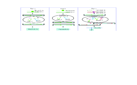
Figure 1: Three types of waveguide-emitter chiral couplings constitute single- and two-qubit photonic gates.

It is expected that the study opens an avenue for photonic quantum computation based on the chiral quantum network cnw . Furthermore, we design a quantum algorithm to perform the supervised learning tasks by properly integrating the realized gates into a circuit. The performance of typical supervised learning tasks is numerically simulated based on gradient descent optimization. Peculiarly, in our framework, the matrix elements representing the single-photon gate show nonlinear relationships with respect to the tunable gate parameters, which are rewarded by the emitter-waveguide interaction. Thanks to this, the encoding of the input data results in the complicated nonlinear mapping, which is known as an essential role for the learning ability. Therefore, it is expected that our work opens up an issue to develop the rich quantum feature mappings QFM ; QCL ; ker by the atoms with various structures interacting with photons in quantum optics. The study represents a fresh potential quantum optics platform for machine learning.

II Chiral-quantum-optics-based photonic quantum computation

We first consider three types of atom-waveguide-chiral couplings as shown in Fig. 1, which constitute essential gates for gate-based photonic quantum computation. The calculations supporting the following main outcomes are shown in the supplementary material.

Photonic single-qubit rotation gate. There is a $\Lambda$-type atom chirally coupled to a pair of waveguides, type a in Fig. 1. The atomic transition $\left|1\right\rangle\leftrightarrow\left|2\right\rangle$ is coupled to the right-moving single photons in the waveguide $m_{0}$ and waveguide $m_{1}$ with strength $g$. An external Laser is introduced to drive the transition $\left|2\right\rangle\leftrightarrow\left|3\right\rangle$. Initially, the atom is in its ground state $\left|1\right\rangle$. Due to the scattering, the single photon moving in the waveguide $m_{0}$ ($m_{1}$) towards the atom is delivered into the waveguide $m_{1}$ ($m_{0}$) with certain probability. The transfer matrix corresponding to this process is

$$R(g,\Omega,\delta_{k},\Delta)=\left[\begin{array}[]{cc}\frac{\delta_{k}\Delta_{k}-\Omega^{2}}{\Delta_{k}(\delta_{k}-i\Gamma)-\Omega^{2}}&\frac{i\Delta_{k}\Gamma}{\Delta_{k}(\delta_{k}-i\Gamma)-\Omega^{2}}\\ \frac{i\Delta_{k}\Gamma}{\Delta_{k}(\delta_{k}-i\Gamma)-\Omega^{2}}&\frac{\delta_{k}\Delta_{k}-\Omega^{2}}{\Delta_{k}(\delta_{k}-i\Gamma)-\Omega^{2}}\end{array}\right]$$ (1)

with $\Omega$ the Rabi frequency of the Laser, $\Gamma=g^{2}$, and $\Delta_{k}=\delta_{k}-\Delta$. The symbol $\delta_{k}$ ($\Delta$) denotes the detuning between the input photon (external Laser) and the corresponding atomic transition.

The qubit is represented by the pair of waveguides. The facts that the single photon with energy $E$ is in the waveguide $m_{0}$ and waveguide $m_{1}$ are described by the two degenerate orthogonal photonic quantum states of the qubit, respectively. The emitter-waveguide interaction plays the role of a rotation on the two states and hence acts as a rotation gate. In the quantum scattering theory Shen , the photonic state is the free state outside the emitter-waveguide interaction ranges. This represents the advantage of the far less stringent operational requirements in the temporal dimension, which can significantly reduce errors coming from the operation in the temporal dimension.

Photonic single-qubit phase gate. There is a $\Lambda$-type atom chirally coupled to the waveguide $m_{0}$, type b in Fig. 1. It is the special case of type a when the atom is decoupled to the waveguide $m_{1}$. The single photon in the waveguide $m_{0}$ gains a phase shift, with the phase tuned by the Laser, i. e.

$$P(g,\Omega,\delta_{k},\Delta)=\left[\begin{array}[]{cc}\frac{\Delta_{k}(\delta_{k}+i\frac{\Gamma}{2})-\Omega^{2}}{\Delta_{k}(\delta_{k}-i\frac{\Gamma}{2})-\Omega^{2}}&0\\ 0&1\end{array}\right].$$ (2)

Photonic two-qubit controlled-rotation and controlled-phase gates. There is a five-level atom chirally coupled to the waveguide $m_{1}$, waveguide $m_{0}^{\prime}$ and waveguide $m_{1}^{\prime}$, type c in Fig. 1. The atomic transitions $\left|1\right\rangle\leftrightarrow\left|2\right\rangle$ and $\left|3\right\rangle\leftrightarrow\left|5\right\rangle$ are driven by the right-moving photons in the waveguide $m_{1}$ with strengths $g$ and $g^{\prime}$, respectively. The transition $\left|2\right\rangle\leftrightarrow\left|3\right\rangle$ is driven by an external Laser. The transition $\left|4\right\rangle\leftrightarrow\left|5\right\rangle$ is driven by the right-moving photon in the waveguide $m_{0}^{\prime}$ and waveguide $m_{1}^{\prime}$ with strength $g^{\prime\prime}$. For simplicity, we assume that all the atom-waveguide coupling strengths are equal to $\sqrt{\Gamma}$ in our scheme. The atom is initialized in the state $\left|1\right\rangle$, and the $m$-th pair of waveguides contains a right-moving photon. We label the two situations that the photon is contained in waveguide $m_{1}$ and in waveguide $m_{0}$ by situation A and situation B, respectively. In situation A, the atom will absorb the photon and then reemit it, meanwhile making the transition $\left|1\right\rangle\rightarrow\left|5\right\rangle$ with probability $P_{conv}$ or maintaining in the state $\left|1\right\rangle$. The former transition corresponds to the inelastic scattering in most cases because of energy conservation. This constitutes a tunable frequency convertor with the conversion efficiency $P_{conv}$. The frequency of reemitted photon and the conversion efficiency can be tuned by the external Laser. The quantum frequency convertor has many critical applications for connecting the quantum systems with different frequencies. In this work, we assume $\omega_{51}=\omega_{32}$, the input photon and the Laser resonantly drive the atom, and the Rabi frequency of the Laser is equal to $\frac{\Gamma}{2}$. The symbol $\omega_{ij}$ denotes the transition frequency between the levels $\left|i\right\rangle$ and $\left|j\right\rangle$. In this case, the atom is determinably in the state $\left|5\right\rangle$ after the elastic scattering. In addition, the reemitted photon gains a phase shift of $\frac{\pi}{2}$. If another single photon is subsequently injected into the waveguide $m_{0}^{\prime}$ ($m_{1}^{\prime}$), it drives the transition $\left|4\right\rangle\leftrightarrow\left|5\right\rangle$.

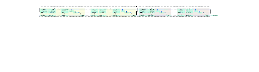
Figure 2: The quantum circuit of machine learning. The gate $R^{(h)}_{j_{1},j_{2},j_{3}}$ ($P^{(h)}_{j_{1},j_{2},j_{3}}$)denotes the gate represented by Type a (Type b), with the corner marks representing different gates as shown in the main text. The gate $X$ is composed by Type c. Limited by the figure length, the $\frac{\pi}{2}$-phase shift in Type c, which is considered in the numerical simulations, is not plotted.

Then it is delivered into waveguide $m_{1}^{\prime}$ ($m_{0}^{\prime}$) with the transfer matrix $\frac{\delta_{k}^{\prime\prime}}{\delta_{k}^{\prime\prime}-i\Gamma}I+\frac{i\Gamma}{\delta_{k}^{\prime\prime}-i\Gamma}X$. The operator $I$ denotes the two dimensional identity matrix, $X$ represents the Pauli-X gate, and $\delta_{k}^{\prime\prime}$ is the detuning between the single photon and the atomic transition $\left|4\right\rangle\leftrightarrow\left|5\right\rangle$. The atom can transit to its initial state by interacting again with the reemitted photon. A candidate for this is to bring in an auxiliary waveguide connecting the waveguide $m_{1}$ with atoms of type a. It is possible that the reemitted photon is routed into the auxiliary waveguide and then is delivered into the waveguide $m_{1}$ by switching the laser for the long optical path. In situation B, the photon does not drive the atomic transition and hence the atom maintains its initial state $\left|1\right\rangle$. If another single photon is subsequently injected into the waveguide $m_{0}^{\prime}$ ($m_{1}^{\prime}$), it is decoupled to the atom. Therefore, type c constitutes a combination of two operations. One is the rotation operation on the photonic state of the $m^{\prime}$-th pair of waveguides, which is controlled by the photonic state of the $m$-th pair of waveguides. The other is the $\frac{\pi}{2}$-phase-shift operation operated on the photon in the waveguide $m_{1}$. Especially, when the transition $\left|4\right\rangle\leftrightarrow\left|5\right\rangle$ is decoupled to either of the $m^{\prime}$-th pair of waveguides, the controlled-rotation gate becomes the controlled-phase gate. In the following learning tasks, we consider the resonant case, i. e. $\delta_{k}^{\prime\prime}=0$, and hence the controlled-rotation gate reduces to the C-NOT gate.

Therefore, the rotation, phase and controlled-rotation and controlled phase gates can be realized by the chiral emitter-waveguide couplings. The operation $R(g,\Omega,\delta_{k},\Delta)$ can also be interpreted as the single-qubit $X$ rotation, i. e. $R(g,\Omega,\delta_{k},\Delta)=e^{-i\frac{\theta}{2}}R_{X}(\theta)$, with $R_{X}(\theta)=\cos(\frac{\theta}{2})I-i\sin(\frac{\theta}{2})X$. The angle $\theta$, which satisfies $\sin\frac{\theta}{2}=\frac{-\Delta_{k}\Gamma}{\sqrt{(\Delta_{k}\delta_{k}-\Omega^{2})^{2}+(\Delta_{k}\Gamma)^{2}}}$ and $\cos\frac{\theta}{2}=\frac{\Delta_{k}\delta_{k}-\Omega^{2}}{\sqrt{(\Delta_{k}\delta_{k}-\Omega^{2})^{2}+(\Delta_{k}\Gamma)^{2}}}$, can be tuned from $0$ to $2\pi$ by the external Laser. Similarly, the operation $P(g,\Omega,\delta_{k},\Delta)$ can be interpreted as the single-qubit $Z$ rotation. More complicated gates can be obtained by the integration of the realized gates. In practice, the imperfect chiral couplings and the atomic dissipations to the other modes except for the guided mode are harmful to the photonic gates. As shown in numerical simulations in the supplemental material, the gates are efficient when the Purcell factor $P\sim\frac{1}{60}$ puer and $\frac{\Gamma_{R}}{\Gamma_{L}}\sim 50$ Sollner , with $\Gamma_{L}$ denoting the coupling strength of the emitter with the left-moving photon in the imperfect chiral case.

III Chiral-quantum-optics-based supervised learning

We proceed to develop an quantum algorithm to perform the supervised learning tasks by integrating the realized photonic gates into a quantum circuit, which can be considered as a chiral network. The quantum circuit, as shown in Fig. 2, is composed by the realized gates operating on $Q$ qubits.

The scheme is decomposed into two parts. Part One contains $L$ layers. There are $N$ rotation gates, composed by type a, sequentially operating on the $m$-th ($m=1...Q$) qubit in each layer. Then the controlled-NOT gates composed by type c are performed to obtain the correlations between the nearest neighbor qubits. Part Two contains $L^{\prime}$ layers. There are one rotation gate composed by type a and one phase gate composed by type b acting on the $m$-th qubit in each layer. Then the nearest neighbor qubits are correlated by nonlocal operations, as done in Part One. To distinguish the parameters belonging to different single-qubit gates of the global circuit, we bring in the indexes to distinguish the different single-qubit gates. For example, we use $\Omega_{j_{1},j_{2},j_{3}}^{(h)}$ to denote the Rabi frequency corresponding to the $j_{2}$-th single-qubit gate, acting on the $j_{1}$-th qubit, in layer $j_{3}$, part $h$.

For a given input set $\{\mathbf{x}_{i}\}$, we label the output function of the learning model and the teacher data with $\{g(\mathbf{x}_{i},\mathbf{\Theta})\}$ and $\{f(\mathbf{x}_{i})\}$, respectively. In supervised learning, one aims to update the parameter $\mathbf{\Theta}$ to make the output function close to the teacher data. We consider that, initially, all the $Q$ qubits are in the state $\left|0\right\rangle$. After the quantum operations represented in Fig. 2, the probability $P$ of the $Q$-th qubit in its state $\left|1\right\rangle$ is measured. Obviously, $P$ is the function with respect to the parameters of the single-qubit gates. We assume that the atomic transition frequencies and the frequencies of guided photons are fixed, while the frequencies and Rabi frequencies of the external Lasers are adjustable. The adjustable parameters are divided into two parts. One part is used to encode the input set and hence labeled by $\mathbf{x}_{i}$. The other part contains the updated parameters and is labeled by $\mathbf{\Theta}$. Then one can label $P\rightarrow P(\mathbf{x}_{i},\mathbf{\Theta,F})$, with $\mathbf{F}$ denoting the set of the fixed gate parameters. In the following numerical simulations, each of the detunings between the input photons and corresponding atomic transitions is the rand number in the range $[-2\Gamma,2\Gamma]$ produced by the computer and then keeps constant. The output function is defined by a linear transformation of $P$, i. e. $g(\mathbf{x}_{i},\mathbf{\Theta,F})=\omega P(\mathbf{x}_{i},\mathbf{\Theta,F})+b$, with $\omega$ and $b$ real numbers. The quadratic cost function, $L=\frac{1}{2}\sum_{i}[g(\mathbf{x}_{i},\mathbf{\Theta,F})-f(\mathbf{x}_{i})]^{2}$ is introduced to measure the gap between the teacher data and the output function. Based on the gradient descent, the parameters are iterated as $\mathbf{\Theta}\leftarrow\mathbf{\Theta}-\nabla_{\mathbf{\Theta}}L$ until the value of the cost function is small enough. The analytical gradients of the measurement with respect to variational parameters can be obtained based on the parameter-shift rules developed in Ref. Mari (see the supplementary material for details).

The input data $\mathbf{x}_{i}$ is encoded in the Laser frequencies of the single-qubit rotation gates in Part One, i. e. $\mathbf{x}_{i}=\mathbf{\Delta^{(1)}}$ with $\mathbf{\Delta^{(1)}}$ the set composed by all the detunings $\Delta^{(1)}_{j_{1},j_{2},j_{3}}$ in Part One. The encoding provides the complicated nonlinearity into the output function with respect to the input data because the elements in the transfer matrix (1) show the nonlinear relationship with $\Delta$. The tensor product structure of the $Q$ qubits results in the tensor of the rotation matrices, which brings in more complicated nonlinearity formally. The nonlocal operations play a key role because the measurement of the $Q$-th qubit is independent of the operations on other qubits if there is no nonlocal operation. These are crucial for the learning ability. The system dimension increases exponentially, i. e. $2^{Q}$, due to the tensor product structure. When the dimension of the system is large enough, it is difficult to calculate by classical computer. For the quantum system, the outcomes are obtained by running the operations and performing the measurements. Quantum computing is expected to perform efficient calculations when the dimension is large, which is one purpose for most quantum algorithms.

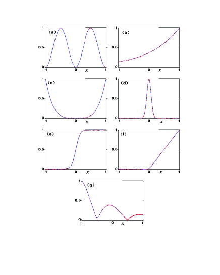
Figure 3: Numerically simulating the performance of regression tasks. The red dots denote the teachers $f(x)$ against the one-dimension input data $x$. The blue solid lines denote the output functions of the learning model against the encoding gate parameters, i. e. $\Delta^{(1)}_{a,b,c}$ with $a=1..Q$, $b=1..N$, and $c=1..L$. The parameters are $L=4$, $N=3$, $Q=4$, $L^{\prime}=8$, $\omega=2$, $b=-0.5$, and $\Gamma$ is taken as a unit. The target functions are: (a) $f(x)=sin^{2}(x\cdot\pi)$, (b) $f(x)=e^{x-1}$, (c) $f(x)=x^{4}$, (d) $f(x)=e^{-x^{2}/0.01}$, (e) $f(x)=\frac{1}{1+e^{-15x}}$, (f) Rectified Linear Unit, (g) $f(x)=|cos(x\cdot\pi)|e^{-(x+1)}$.

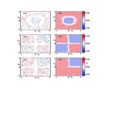
Figure 4: Numerically simulating the performance of classification tasks. (a), (c), and (e) represent the teachers. The blue dots indicate class $0$ with $f(x_{1},x_{2})=0$, while the red triangles indicate class $1$ with $f(x_{1},x_{2})=1$. The corresponding learning results, i. e. the output function $g(x_{1},x_{2},\Theta)$ against the inputs, are represented in (b), (d), and (f), respectively. The value of the output function that is smaller (lager) than 0.5 indicates the class $0$ ($1$). The parameters are $L=4$, $N=6$, $Q=4$, $L^{\prime}=8$, $\omega=1$, $b=0$, and $\Gamma$ is taken as a unit.

From the recent viewpoint raised in ker , the quantum operations of Part One could be understood as a recent new concept of quantum feature mapping QFM ; QCL ; ker , and the measurement bases are altered by variable parameters in Part Two. Obviously, if the $\Lambda$-type emitters in Part One are replaced by the emitters with other structures, different nonlinear mappings resulting from the encoding can be obtained. It is possible to obtain rich quantum feature mappings by the atom with various structures interacting with the photons. The interaction between the atom with different structures and few photons is one of the research topics in quantum optics. This implies the issue to develop the quantum feature mapping by the platform of quantum optics.

We proceed to numerically simulate the performance of two prototypical supervised learning tasks, i. e. regression and classification. The performance of the regression tasks is shown in Fig. 3. For simplicity, we consider that all the gates are operated in the ideal case. From the encoding manner defined above, we take $\Delta_{a,b,c}^{(1)}=x$, with $a=1...Q$, $b=1...N$ and $c=1...L$. All the parameters belonging to $\mathbf{\Theta}$ are random numbers produced by the computer in the initial time and then updated during the training in both the regression and classification tasks. The variable parameters in Part Two adjust the rotation angles of $R_{X}(.)$ and $R_{Z}(.)$. The periodicity of the rotations can reduce the values of the exploded gradients and meanwhile alters the gradient direction, which efficiently reduce the possibility of the local minimum. In Fig. 3(a)-(d), the scheme well fits the typical nonlinear functions. The target functions in Fig. 3(e) and (f) are the typical activation functions used in neuron network. It implies that the scheme may perform complicated learning tasks without bringing in the external nonlinear function, such as the sigmoid function in the binary classification task. The target function in Fig. 3(g) is a decay function, the similar lineshape to which is common in quantum optics. For example, the evolution of the atomic population in a structured environment with memory mem ; mem2 . Machine learning has been recently considered as a promising tool for the research on quantum technology. It is expected that the scheme can serve quantum technology. The simulations show that the framework can output a wide variety of functions with respect to the simple input.

The numerical simulation of performing the binary classification tasks is shown in Fig. 4. When the training input data is the $2$-dimensional vector, the $i$-th input data is denoted by $\mathbf{x}_{i}=(x_{i,1},x_{i,2})$. Then the gate parameters for encoding should be divided into two halves. One encodes $x_{i,1}$ and the other encodes $x_{i,2}$. We assume that each layer in Part One contains $6$ single-qubit rotation gates operating on the $m$-th ($m=1..Q$) qubit, i. e. $N=6$. The input $x_{i,1}$ is encoded in the Laser frequencies of the 1st, 3rd and 5th rotation gates while $x_{i,2}$ is encoded in the Laser frequencies of the 2nd, 4th and 6th rotation gates, i. e. $\Delta_{j_{1},j_{2},j_{3},1}=x_{i,2-(j_{2}\ mod\ 2)}$ with $j_{2}\ mod\ 2$ the remainder of $j_{2}\$divided by $2$. The outcomes show that the framework well performs different typical classification tasks.

IV Discussions

In summary, the photonic quantum computation has been realized based on chiral quantum optics. Four elementary single- and two-qubit photonic gates for photonic quantum computation are mediated by multi-level atoms chirally coupled to the waveguides. More complex gates used in quantum computation can be achieved by integrating the proposed gates. The tunable gate parameters are composed by the parameters of the external Lasers, which is employed to drive the emitters. Moreover, we develop the quantum machine learning algorithm by integrating the realized gates into a quantum chiral net. Some typical simple nonlinear supervised learning tasks are verified by numerically simulating the performance with classical computer. During the training, the gate parameters are tuned according to the gradient descent optimization. It is reasonable that the scheme would be generalized to a high-dimensional complex structure in practice, which is difficult for the classical calculations, for various tasks. In our numerical simulations, the ideal gates are considered for simplicity. In reality, the atomic decay and imperfect chiral coupling influence the gate efficiency. Especially, the latter, which brings difficulties to the simulation, would introduce complicated interferenceyanwb . Therefore, the imperfect chiral coupling may improve the learning ability, which is hoped to be verified experimentally in future. Currently, benefiting from the chiral single-photon switch, a novel realization of the C-NOT gate operating on the state of atom-like scheme is proposed zhouy . The potential realization of chiral photon emitter is analyzed in detail based on different practical implementations, such as the optical photon interacting with a NV center, the quantum dot interfaced to a semi-conductor waveguide, and the guided mode composed by surface plasmon. It implies the potential implementation for our scheme. Our work paves the way for the implementation of photonic quantum computation, especially for quantum machine learning.

- (1) M. I. Jordan and T. M. Mitchell, Science, 349, 255 (2015).
- (2) M. A. Nielsen and I. L. Chuang, Quantum computation and quantum informations (10th Anniversary Edition), Cambridge University Press, (2010).
- (3) P. W. Shor, SIAM J. Comput. 26, 1484 (1997).
- (4) L. K. Grover, Proceedings of 28th Annual ACM Symposium on the Theory of Computing, pp: 212 (1996).
- (5) P. Wittek, Quantum machine learning: What quantum computing means to data mining, Academic Press, (2014).
- (6) J. Biamonte, P. Wittek, N. Pancotti, P. Rebentrost, N. Wiebe, and S. Lloyd, Nature, 549, 195 (2017).
- (7) V. Dunjko, and H. J. Briegel, Rep. Prog. Phys. 81, 074001 (2018).
- (8) P. Rebentrost, M. Mohseni, and S. Lloyd, Phys. Rev. Lett. 113, 130503 (2014).
- (9) S. Lloyd, M. Mohseni, and P. Rebentrost, 10, 631 (2014).
- (10) S. Lloyd and C. Weedbrook, Phys. Rev. Lett. 121, 040502 (2018).
- (11) M. H. Amin, E. Andriyash, J. Rolfe, B. Kulchytskyy, and R. Melko, Phys. Rev. X, 8, 021050 (2018).
- (12) M. Schuld and N. Killoran, Phys. Rev. Lett. 122, 040504 (2019).
- (13) K. Mitarai, M. Negoro, M. Kitagawa, and K. Fujii, Phys. Rev. A, 98, 032309 (2018).
- (14) C. Blank, D. K. Park, JK. K. Rhee, and F. Petruccione, npj Quantum Inf. 6, 41 (2020).
- (15) M. Schuld, arXiv:, 2101.11020 (2021).
- (16) V. Havlíček, A. D. Cócoles, K. Temme, A. W. Harrow, A. Kandala, J. M. Chow, and J. M. Gambetta, Nature, 567, 209 (2019).
- (17) P. Lodahl, S. Mahmoodian, S. Stobbe, A. Rauschenbeutel, P. Schneeweiss, J. Volz, H. Pichler, and P. Zoller, Nature, 541, 473 (2017).
- (18) I. Söllner, S. Mahmoodian, S. Hansen, L. Midolo, A. Javadi, G. Kiršanskè, T. Pregnolato, H. El-Ella, E. H. Lee, J. Song, S. Stobbe, and P. Lodahl, Nature Nanotech. 10, 775 (2015).
- (19) C. Sayrin, C. Junge, R. Mitsch, B. Albrecht, D. O´Shea, P. Schneeweiss, J. Volz, and A. Rauschenbeutel, Phys. Rev. X, 5, 041036 (2015).
- (20) M. Scheucher, A. Hilico, E. Will, J. Volz, and A. Rauschenbeutel, Science, 354, 1577 (2016).
- (21) H. Pichler, T. Ramos, A. J. Daley, and P. Zoller, Phys. Rev. A, 91, 042116 (2015).
- (22) J. T. Shen and S. Fan, Phys. Rev. A, 76, 062709 (2007).
- (23) P. Lodahl, S. Mahmoodian, and S. Stobbe, Rev. Mod. Phys. 87, 347 (2015).
- (24) A. Mari, T. R. Bromley, and N. Killoran, Phys. Rev. A, 103, 012405 (2021).
- (25) B. M. Garraway, Phys. Rev. A 55, 2290 (1997).
- (26) B. M. Garraway, Phys. Rev. A 55, 4636 (1997).
- (27) W.-B. Yan, W.-Y. Ni, J. Zhang, F.-Y. Zhang, and H. Fan, Phys. rev. A, 98, 043852 (2018).
- (28) Y. Zhou, D.-Y. Lv, and W.-Y. Zeng, Photonics Res. 9, 405 (2021).