Identification of novel organic polar materials: A study combining importance sampling with machine learning

Ayana Ghosh ghosha@ornl.gov Center for Nanophase Materials Sciences and Computational Sciences and Engineering Division, Oak Ridge National Laboratory, Oak Ridge, Tennessee 37831, USA Department of Materials Science

\&

Engineering and Institute of Materials Science, University of Connecticut, Storrs, Connecticut 06269, USA Dennis P. Trujillo Department of Materials Science

\&

Engineering and Institute of Materials Science, University of Connecticut, Storrs, Connecticut 06269, USA Subhashis Hazarika Palo Alto Research Center, Palo Alto, California 94304, USA Elizabeth Schiesser Department of Biomedical Engineering, University of Connecticut, Storrs, Connecticut 06269, USA M. J. Swamynathan Department of Physics and Nanotechnology, Faculty of Engineering and Technology, SRM Institute of Science and Technology, Kattankulathur - 603 203, Tamil Nadu, India Saurabh Ghosh Department of Physics and Nanotechnology, Faculty of Engineering and Technology, SRM Institute of Science and Technology, Kattankulathur - 603 203, Tamil Nadu, India Jian-Xin Zhu Theoretical Division, Los Alamos National Laboratory, Los Alamos, New Mexico 87545, USA Center for Integrated Nanotechnologies, Los Alamos National Laboratory, Los Alamos, New Mexico 87545, USA Serge Nakhmanson serge.nakhmanson@uconn.edu Department of Materials Science

\&

Engineering and Institute of Materials Science, University of Connecticut, Storrs, Connecticut 06269, USA Department of Physics, University of Connecticut, Storrs, Connecticut 06269, USA

Abstract

Recent advances in the synthesis of polar molecular materials have produced practical alternatives to ferroelectric ceramics, opening up exciting new avenues for their incorporation into modern electronic devices. However, in order to realize the full potential of polar polymer and molecular crystals for modern technological applications, it is paramount to assemble and evaluate all the available data for such compounds, identifying descriptors that could be associated with an emergence of ferroelectricity. In this work, we utilized data-driven approaches to judiciously shortlist candidate materials from a wide chemical space that could possess ferroelectric functionalities. An importance-sampling based method was utilized to address the challenge of having a limited amount of available data on already known organic ferroelectrics. Sets of molecular- and crystal-level descriptors were combined with a Random Forest Regression algorithm in order to predict spontaneous polarization of the shortlisted compounds. First-principles simulations were performed to further validate the predictions obtained from the machine learning model.

I introduction

Ferroelectric materials are widely employed in a variety of technological applications, including acoustic, nonlinear-optic and electromechanical devices — i.e., sensors, actuators and transducers — as well as in pyroelectric arrays, nonvolatile memories, and high- $k$ dielectric components for microelectronics. Perovskite ABO₃-type metal-oxide ceramics, such as BaTiO₃, PbTiO₃, KNbO₃, or related solid solutions, such as PbZr_1-xTi_xO₃ (PZT), usually exhibit the strongest spontaneous polarization, as well as piezoelectric, and pyroelectric response. However, the usefulness of oxide ceramics is limited by their substantial weight, brittleness, toxicity (e.g., in lead-containing compounds) and considerable costs of material synthesis and device manufacturing.Choi et al. (2004); Lee et al. (2005) On the other hand, molecular- or polymer-based ferroelectrics, while displaying more modest polar properties, are usually lightweight, flexible and environmentally friendly.Lovinger (1983); Furukawa (1989); Kepler and Anderson (1992); Nalwa (1995); Eberle et al. (1996); Samara (2001) A wide range of practical and inexpensive prescriptions is available for their growth and processing as either bulk materials or nanostructures.

In order to fully realize the potential of polar polymer- and molecular-based materials for modern technological applications, it is paramount to acquire detailed molecular-level understanding of mechanisms governing the emergence of ferroelectricity in them. It is noteworthy that some of the most well known ferroelectric compounds,Horiuchi and Tokura (2008) e.g., Rochelle salt, in which ferroelectricity was originally discovered, or NaNO₂ that exhibits incommensurate structural distortions,Heine and McConnell (1984) can be classified as molecular crystals. Compared to the transition-metal oxide counterparts, the origins of ferroelectric behavior in such materials are more diverse and not as exhaustively investigated.Louis et al. (2018) Therefore, reliable paths to enhancement and control of their useful properties still largely remain to be charted out.

Despite the existence of various physical mechanisms that could potentially induce ferroelectricity in polymer and molecular-based materials — in addition to the displacive mechanism which dominates in ceramics — it continues to be rare, a ‘one-off’ or spurious effect. Lessons learned by some of the authors when studying DIPA-X Louis et al. (2018) and PVDF-based Ghosh et al. (2018) families of electroactive compounds provided some insight into why this may be so. Even though individual molecular units may be highly polar, when they are assembled into a periodic crystal structure, there is no guarantee that it will be ferroelectric: [A] Unit arrangements promoting cancellation of large individual dipole moments are likely to form, resulting only in weak or complete absence of polarization; [B] Built-in energy barriers for dipole reorientation may be too high to allow ‘easy’ polarization switching among multiple possible directions. In the latter case, the material may formally be ferroelectric, but the associated enormous coercive fields make applications impractical.

Although specific pieces of knowledge useful for successful cultivation of ferroelectric properties in polymer and molecular-based systems may remain elusive — unquestionably, because of the structural richness of the involved material families and great complexity of the underlying physical mechanisms — this problem is highly amenable to probing with generic machine learning (ML) and data mining approaches.Sattari et al. (2021) The main idea is to utilize the available information for the already known ferroelectric molecular- and polymer-based compounds to uncover any general commonalities in and connections among their structure, chemical makeup, properties and performance, identifying a small number of simple descriptors that ‘point’ to ferroelectric behavior. These descriptors can then be used to predict the likelihood of such behavior in other molecular- and polymer-based compounds, whether fictitious or already synthesized.

Engaging in such a study involves a number of difficulties, with the most obvious being: (a) Scarcity of the available data on the already known molecular and polymeric ferroelectrics, as there are just not too many of them — less than a hundred, which stipulates the types of ML algorithms that could used; (b) Lack of any standards on how such data is organized and curated, i.e., individual research groups report whatever they feel is important in each particular case, rather than a prescribed set of descriptors, plus different groups have dissimilar quality standards for what is considered ‘reliable data.’ On the other hand, for compound crystal systems that could be readily separated into individual molecule-based structural units, preexisting libraries of numerous chemical descriptors could be readily applied for characterization of these units. Naturally, such chemical descriptors acting on the molecular level can be combined with global, crystal-level descriptors.

Guiding principles for the selection of prospective ferroelectric materials: For the purposes of this, or a similar (more detailed) investigation, the following natural connections between the material structure / properties and the desired ‘ferroelectric propensity’ could be used for shortlisting the most attractive target compounds from a larger pool of possible candidates. (i) Existence of multiple polymorphs for the same compound, some of which are non-centrosymmetric and polar, while others are centrosymmetric and non-polar. (ii) Energetic closeness of the polar and aristotype non-polar phases, meaning that these phases cannot be drastically structurally different. (iii) Existence of well-behaved transformation paths connecting different variants of the polar phases, indicating feasibility of ferroelectric switching among them. While criterion (i) is based purely on symmetry considerations and thus is easy to include into a data-driven workflow, criteria (ii) and (iii) may require deployment of extra and possibly substantial computational efforts, e.g., to evaluate relative energy differences between the phases, as well as probe possible transformation paths connecting them. In this study, we aimed to avoid, whenever possible, doing any heavy atomistic-level calculations of this sort. Although, clearly, for each prospective ferroelectric identified, these (and other) calculations would be necessary to characterize its behavior with confidence, here our goal was to spin out multiple (but not too many!) reasonable guesses for such prospective compounds and provide rough, but computationally cheap estimates of their likely properties.

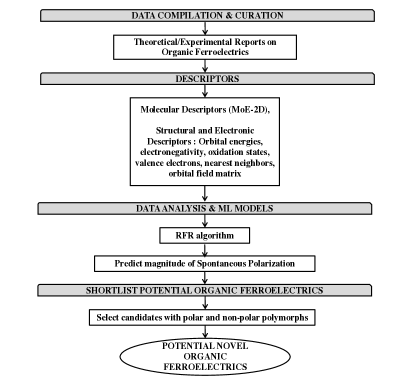
In what follows, we demonstrate how we have addressed some of the challenges stated above, showcasing an original data-driven and ML approach that can judiciously choose target materials likely to exhibit ferroelectricity from a wide chemical space of different molecular- and polymer-based candidate compounds. In conjunction, we present a number of crystal- and molecular-level descriptors that were recognized as important for predicting ferroelectric behavior. In addition, we highlight the utilization of traditional ML algorithms for constructing a model that can estimate the magnitude of spontaneous polarization in the identified target materials without performing computationally expensive atomistic-level calculations. The flowchart showing connections between the main developmental stages of this study is presented in Fig. 1.

Refer to caption — Figure 1: A flowchart of main stages involved in development of the selection process for identifying molecular- and polymer-based materials with ferroelectric propensity. Primary stages are shown as grey rectangles, while any necessary secondary stages are represented by white rectangles. All methodological details involved in implementation of each stage are presented in Sec. II.

II Methods

II.1 Data Compilation and Curation

As a starting point of this study, a dataset, called in what follows ‘Dataset I,’ was compiled and curated, containing data records for most already known molecular- and polymer-based ferroelectrics reported in the literature.Horiuchi and Tokura (2008); Lines and Glass (2001); Ye et al. (2018) Table I in the Supplementary Material lists stoichiometric formulas and SMILEs (simplified molecular-input line-entry system) strings for molecular units of all of the collected entries, with the latter providing more detailed description for the compound structure and chemical makeup. Other properties collected by curating the literature were lattice parameters for unit cells, molecular weight (g/mol), melting temperature (^∘C), density (g/cm³), polarization values (C/m²), transition temperature (^∘C) and space groups. We note that for some molecular systems present in Dataset I the complete information could not be obtained. Therefore, the initial descriptor space for these compounds was built using only SMILEs representations, while assuming cubic unit cells. Ideally, descriptions of the structure of these molecular systems should be clarified (e.g., by using first-principles theory computations for structural optimization), but such efforts are beyond the scope of this work.

At the time of this writing, Dataset I contains information for a total of 76 molecular systems, with reported origins for the emergence of ferroelectricity including electronegativity differences between atoms, secondary interactions such as hydrogen bonding, as well as lattice-distortion driven structural instabilities. The chemical nature and structure of the dataset entries are extremely diverse and include molecular and polymer crystals, oligomers, co-crystals, clathrates, charge-transfer complexes and derivatives of metal-organic frameworks. Only systems that have been reported by multiple research groups and could be verified by comparison with common databases — in particular, Cambridge Structural Database (CSD)Groom et al. (2016) — were included in Dataset I. CSD utilizes the R-factor metric to determine the quality of structural data, with the average value of considerable R-factor for small organic molecules (like ones used in Dataset I and for shortlisting potential organic ferroelectrics) being $<$ 0.05.

II.2 Descriptors

For each of the Dataset I compounds, we have computed sets of molecular- and crystal-level descriptors. For the former, standard computational Molecular Operating Environment (MOE)Clark et al. (2006); Moe 2D chemical descriptors were used, while descriptors relying on a three dimensional shape of the investigated molecule were excluded to avoid adding any potential ambiguities to the descriptor space. Crystal-level descriptors, as implemented in a Python library,Ward et al. (2018); Ricci et al. (2020); Ward et al. (2016) included atomic orbital information, i.e., energies of highest occupied molecular orbital (HOMO) and lowest unoccupied molecular orbital (LUMO), orbital energies, types of and distances between atomic sites, fractions of nearest neighbors for each atomic and bond type. Statistical data on electronegativity differences between anions and cations, oxidation states of all atoms, valence orbital attributes, such as mean number of electrons in each shell, and orbital field matrix descriptions of the chemical environment of each atom in the unit cell, based on the group numbers, row numbers, distances between coordinating atoms, and Voronoi polyhedra weights were also included.

II.3 ML Models for Predicting Polarization

A family of ML models was constructed utilizing the computed sets of molecular- and crystal-level descriptors. Initial models included all the descriptors, while consecutive ones were built on only 10 most important descriptors (combined from both sets) as identified by the ML algorithm. The models are constructed based on the best set of hyperparameters after performing full grid-search optimization.

The main target property to be predicted was the magnitude of spontaneous polarization in the compound / system of interest. The Random Forest Regression (RFR) algorithm was employed as implemented in scikit-learn Pedregosa et al. (2011) to construct the models. In general, regression-based algorithms were preferred over classification-based ones, as the endpoint of interest — such as, e.g., magnitude of the spontaneous polarization — is continuous in nature. The choice of RFR, in comparison to other regression-based algorithms, was motivated by its performance in the previous studiesGhosh et al. (2020, 2019) when applied to datasets of small size, as well as its capability to rank utilized descriptors by importance. This feature of the RFR algorithm proved to be essential in this investigation, allowing us to identify the likely physical underpinnings that enable ferroelectricity in molecular and polymeric systems.

II.4 Descriptor Ranking for Polarization Prediction

An analysis of the relative importance of each descriptor (belonging to either molecular- or crystal-level descriptor set) was performed utilizing the RFR algorithm feature importance ranking to shortlist the descriptors useful for predicting polarization. The feature importance score produced by RFR represents the decrease in the weighted impurity (variations for regression type of algorithm) over all trees for every feature. As determined, top ten ranked molecular- and crystal-level descriptors provide some physical insight into the structural and chemical properties that may influence polar behavior.

Table 1: Top ten crystal-level descriptors important for predicting polarization as determined by the RFR algorithm feature importance ranking of the descriptor set. Descriptors are ordered in descending order of importance.

Descriptor	Extended Definition
MagpieData mean NdUnfilled	Mean number of unfilled $d$ valence orbitals among elements
MagpieData minimum GSbandgap	Minimum value of the DFT bandgap of elemental solid among elements in composition
vpa	Volume per atom of the crystal structure
MagpieData range Row	Range of the row on periodic table which each element in the composition belongs to
MagpieData avg dev NUnfilled	Average deviation of unfilled valence orbitals among elements
MagpieData avg dev NpUnfilled	Average deviation of number of unfilled $p$ orbitals among elements in composition
MagpieData mean Electronegativity	Mean value of electronegativity among elements in composition
MagpieData avg dev NpValence	Average deviation of unfilled $p$ valence electrons among elements
MagpieData avg dev NdValence	Average deviation of filled $d$ orbitals among elements in composition

For the crystal-level descriptors, it was observed that descriptors representing valence electrons and elemental electronegativity in composition contributed greatly to predicting the polarization of molecular compounds (see Table 1). This is expected since differences in electronegativity between neighbor atoms give rise to local dipole moments which then sum up to produce net polarization in the crystal environment. These descriptors can be further related to the presence of nitrogen, hydrogen and oxygen bonds with metals, such as rhenium and bromine, and, therefore, the propensity of these particular elements to exhibit a variety of highly electropositive oxidation states. Finally, descriptors representing the crystal volume, average number of unfilled $p$ and $d$ orbitals, as well as deviations among them in a molecular crystal were shown to be relatively important to predicting polarization.

Table 2: Top ten molecular-level descriptors important for predicting the polarization as determined by the RFR algorithm feature importance ranking of the descriptor set. Descriptors are ordered in descending order of importance.

Descriptor	Extended Definition
ATS1m	Broto-Moreau autocorrelation weighted by mass
GATS1v	Geary autocorrelation weighted by van der Waals volumes
ATSC1p	Centered Broto-Moreau autocorrelation weighted by probabilities
maxsssCH	Max atom type electronic state -CH-
ETA_dPsi_B	Measure of hydrogen bonding propensity
ATSC2p	Centered Broto-Moreau autocorrelation weighted by probabilities
maxsI	Max atom type electronic state for I
SpMax3_Bhm	Largest absolute eigenvalue of Burden modified matrix wighted by relative mass
AATSC2m	Average centered Broto-Moreau autocorrelation weighted by mass
AATS1m	Average Broto-Moreau autocorrelation weighted by mass

Relative importance of the molecular-level 2D descriptors was also determined in the same fashion. As shown in Table 2, descriptors representing topological distribution of mass, van der Waals volumes, and probabilities (associated with Broto-Moreau and Geary autocorrelationsArthur et al. (2016) of these parameters) were identified as important for predicting polarization. Other important features identified by this analysis included electronic states related to C-H and I bonding, and molecular propensity to form hydrogen bonds. This indicates that the presence of excess H atoms, as well as the presence of iodine (which is highly electronegative), contributes to the polar strength of molecular units comprising the crystal. We note that the molecular-level set descriptors were not considered in the final model for predicting polarization, since they were not found to be highly important for the target property prediction.

II.5 Data Analysis and Improvement of the ML Models

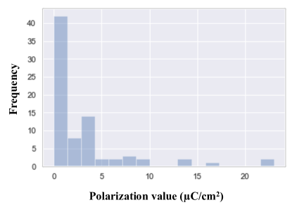
A histogram plot of reported spontaneous polarizations exhibited by the compounds comprising Dataset I is shown in Fig. 2. From this data, it is evident that in addition to being limited in size, Dataset I is strongly skewed or biased towards systems with rather low polarization magnitudes. That is not entirely unexpected, considering that molecular- or polymer-based ferroelectric compounds usually have smaller polarization, compared to their ceramic counterparts. In this situation, an infusion of a substantial number of additional data entries representing systems possessing high spontaneous polarization is required to remove the bias in the data. In general, training predictive ML models on well-balanced data produces better prediction accuracy, compared to using data that is unbalanced.Kaur et al. (2019)

Since the list of already known ferroelectric compounds has been greatly exhausted in the process of assembling Dataset I, we employed an importance samplingNeal (2001) based approach to generate additional synthetic data points with high polarization values — which was accomplished by assigning greater importance to high-polarization instances that have low occurrences in Dataset I. Such statistical strategies, allowing for an infusion of additional samples around low occurrence training data instances, are widely used to address the problem of unbalanced training data in different ML modeling strategies.Chawla et al. (2002)

To generate a balanced version of Dataset I using the importance sampling approach, we had to define a range of polarization magnitudes that is considered important for our analysis. We set the lower boundary of this range to 5 $\mu$ C/cm², as Fig. 2 clearly shows that there are few data instances present in Dataset I with polarizations greater than this value. This lower boundary to generate the samples can be picked in a randomized manner. However, if significant number of original data points do not satisfy the criteria, the new samples generated will be biased towards low frequency values. Lack of variance in such newly generated data points will not help to improve the accuracy of the constructed ML model. Hence, a use of higher threshold of polarization value, e.g., 0 $\mu$ C/cm² or above (only less than 10 data points available in Dataset I with such polarization values) will not yield meaningful samples falling under the range of polarization values of interest.

High dimensionality of the involved descriptor space ( $\sim$ 1,000) introduces difficulties in generating coherent samples from such large multivariate distributions. We note that this large space was initially constructed by combining all possible descriptors and then filtered down on the ML model building stage to contain only descriptors that were highly ranked by their importance. However, during the sample generation stage, we kept all descriptors in their original form to avoid missing any relevant information. To reduce the dimensionality of the descriptor space, we applied Principal Component Analysis (PCA)Abdi and Williams (2010) that projects high-dimensional features (descriptors) to orthogonal, mutually independent dimensions called principal components (PC) by performing an eigen-decomposition of the covariance matrix in the descriptor space. The resulting eigenvectors correspond to the orthogonal PC dimensions. An advantage of using a linear transformation model like PCA is that an inverse transformation can be performed to move from the mutually independent PC space to the high-dimensional descriptor space.

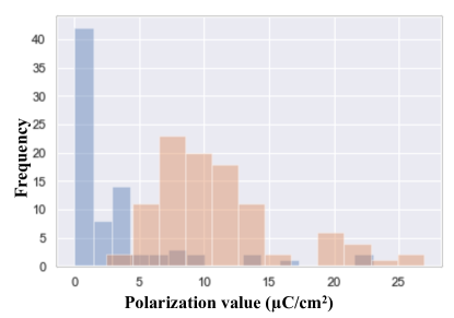
After transforming the high-dimensional descriptor space to low-dimensional PC space with PCA, we generated multiple random samples for the independent PC dimensions. On that sampling step, we first used a kernel density estimate (KDE)Scott (2018) model (with gaussian kernels) to approximate the individual distributions of the independent PCs. We then produced 100 new samples from this KDE distribution and projected them back to the original high-dimensional descriptor space, utilizing the inverse transformation property of PCA. This resulted in 100 new data points that are likely to have polarization values above 5 $\mu$ C/cm². Orange colored bars in Fig. 3 represent the distribution of polarization magnitudes corresponding to these new 100 synthetically created data instances. These new samples were combined with the (unbalanced) Dataset I to create a relatively balanced dataset, called in what follows ‘Dataset II,’ that includes more data instances possessing high polarization values. Note that fictitious samples generated by this procedure were used exclusively to train the ML models, while any test sets consisted only of unaltered original data collected for the actual materials.

III Results and Discussion

III.1 Predicting Ferroelectric Polarization

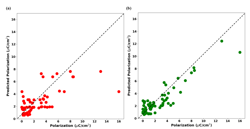
The first iteration of ML models for predicting ferroelectric polarization was built on Dataset I, with one model constructed utilizing molecular-level descriptors only and the other using only crystal-level descriptors. The average RMSEs of these ML models for predicting spontaneous polarization were close to 2.16 $\mu$ C/cm². On the next iteration, an improved model utilizing 10 most important descriptors taken from the combined set of molecular- and crystal-level descriptors was constructed, with the average RMSE of 1.96 $\mu$ C/cm². The range of polarizations was 1–15 $\mu$ C/cm², with most falling below 5 $\mu$ C/cm².

To improve the predictive accuracy of the original ML models, we constructed the third iteration of models employing Dataset II.

It is evident that utilization of the importance sampling approach to un-bias Dataset I improved the predictive quality of the models, reducing the average test set RMSE error to 1.29 $\mu$ C/cm², while also decreasing the overfitting. The parity plots for the best models constructed using Datasets I and II are shown in Fig. 4.

We note that it is possible to create different variants of Dataset II by changing the lower boundary of the ‘important polarization’ range to a value that is higher than 5 $\mu$ C/cm². However, due to much smaller number of reported structures with polarization $>10$ $\mu$ C/cm², samples generated for datasets with large ‘important polarization’ cut-offs will be too similar in nature, therefore not contributing any substantial new information to the dataset. Consequently, any ML models constructed using such datasets will not have their predictive accuracy significantly improved. A different strategy may involve building ML models on datasets that aggregate only those compounds that have the same mechanism for developing ferroelectricity. That approach can further improve prediction accuracy, but at present such partitioning reduces the original dataset to subsets of less than 20 entries in size.

Table 3: Potential organic ferroelectrics for which only 2 structural phases are present in the CSD. Molecular formulas, canonical SMILEs and predicted spontaneous polarization values (in

\mu

C/cm²) are provided. The polarization values have been reported up to three digits after the decimal to avoid rounding errors.

Molecular Formula	Canonical SMILE	$\|\mathbf{P}_{s}\|$
C₁₀H₁₅N₅O	CC(CCNC1=NC=NC2=C1NC=N2)CO	1.476
C₁₀H₆O₈	C1=C(C(=CC(=C1C(=O)O)C(=O)O)C(=O)O)C(=O)O	2.069
C₁₃H₂₁NO₈	CCOC1C=C(OC(C1NC(=O)C)C(C(CO)O)O)C(=O)O	1.747
C₁₃H₂₁N₅	C1CCC(C1)C2=CC(=NC(=N2)N)N3CCC(C3)N	7.098
C₁₃H₇N₃O	C1=CC(=CN=C1)OC2=CC(=C(C=C2)C#N)C#N	1.586
C₁₅H₁₀N₂O₆	COC(=O)C1=C2C(=NC3=C(N2)C(=O)C=C(C3=CO)O)C(=O)C=C1	1.651
C₁₆H₁₄F₃NO₂	C1CC2=CC3=C(C4=C2N(C1)CCC4)OC(=O)C=C3C(F)(F)F	2.024
C₁₇H₁₉N₅O₄	C1C(C(OC1N2C=NC3=C2N=C(N=C3OCC4=CC=CC=C4)N)CO)O	1.701
C₁₈H₂₀N₆O₃	CC1(N=C(N=C(N1C2=CC(=CC=C2)OCC3=CC(=CC=C3)[N+](=O)[O-])N)N)C	1.572
C₁₉H₁₁NO₃	C1=CC=C(C=C1)C=CC2=NOC3=C2C(=O)C4=CC=CC=C4C3=O	1.750
C₁₉H₁₂BF₂N₃O	B(C1=C(N=CC=C1)F)(C2=C(N=CC=C2)F)OC3=CC=CC4=C3N=CC=C4	1.987
C₁₉H₂₂N₂O₃C₂H₆O	CC1=NOC(=C1)CCCCCCCOC2=CC=C(C=C2)C3=NC(CO3)CO	1.493
C₁₉H₃₀O₇	CC(C)(CO)CO.C1=CC=C2C(=C1)C(=O)OC2=O.C(CCCO)CCO	1.403
C₂H₃NO₃	C(=O)(C(=O)O)N	4.347
C₂H₅NO	CC(=O)N	3.342
C₂₀H₂₂O₇H₂O	CC(=O)CC1CCC(=O)C=CC(=O)OC(CCC(=O)C=CC(=O)O1)CC(=O)C	1.704
C₂₀H₂₇F₃O₃	C(CCC(F)(F)F)CC=CCC=CCC=CC=CC(=O)CCCC(=O)O	1.671
C₂₁H₃₆O₅	CCCCCC(C=CC1C(CC(C1CC=CCCCC(=O)OC)O)O)O	1.238
C₂₂H₁₂N₂O₄	C1=CC=C2C(=C1)C(=O)OC(=N2)C3=CC=C(C=C3)C4=NC5=CC=CC=C5C(=O)O4	1.851
C₂₃H₂₅F₃N₂O₃	C1CN(CC(C1C2=CC=C(C=C2)O)F)C3CCN(C3=O)CC4=CC=C(C=C4)OC(F)F	1.783
C₂₄H₂₈N₆O₂	CCCCOC1=CN=CC(=C1)C2=NN=C3N2C4=C(C=CC(=C4)CN5CCOCC5)N=C3C	1.298
C₂₄H₃₄O₁₅	CC(=O)OCC1C(C(C(C(O1)C2(C(CCOC2COC(=O)C)OC(=O)C)O)OC(=O)C)OC(=O)C)OC(=O)C	1.805
C₂₄H₃₅N₃	CC1=C2CCCCN2C(=C1)C3=CC=C(C=C3)N(C)CCCN4CCCCC4	7.098
C₂₅H₃₁N₃O₂	CC(C)N1CCC(CC1)NC(=O)C2=CC3=CC=CC=C3N2CC4=CC(=CC=C4)OC	1.298
C₂₆H₂₂BNO₃	[B-]12([N+]3=C(C=CC=C3C4=C(O1)C=CC(=C4)C)C5=C(O2)C=CC(=C5)C)C6=CC=C(C=C6)OC	1.213
C₂₇H₁₆	C1C2=C3C(=CC=C2)C4=CC=CC5=C4C(=CC=C5)C3=C6C1=C7C=CC=CC7=C6	6.804
C₂₈H₂₀O₆	C1=CC(=CC=C1C=CC2=C3C(=CC(=C2)O)OC(=C3C4=CC(=CC(=C4)O)O)C5=CC=C(C=C5)O)O	1.876
C₂₈H₂₈B₂N₄	[B-]12(CC([B-](C3=[N+]1C=CN3C)([N+]4=C2N(C=C4)C)C5=CC=CC=C5)C6=CC=CC=C6)C7=CC=CC=C7	6.639
C₂₉H₄₅NO₅	CC(C)C(=O)OC(C)C=CC(=O)NC1CCC(CC1)CC=C(C)C=CC2CC3(CC(O2)(C)C)CO3	1.255
C₃₂H₂₄O₃	CC1=C2C3=C(C=CC=C3O)C(C4=C2C(=CC=C4)O1)CC(=C5C6=CC=CC=C6C7=C5C=C(C=C7)O)C	1.298
C₃₂H₂₆O₃	COC1=CC=C(C=C1)C2=CC(=C(C=C2)C3=CC=CC=C3)C4=CC=CC=C4OC5=CC=C(C=C5)OC	1.214
C₃₂H₃₆N₂O₅	CC1CC=CC2C3C(O3)(C(C4C2(C(=O)C=CC(=O)C(C(=C1)C)O)C(=O)NC4CC5=CNC6=CC=CC=C65)C)C	1.262
C₃₆H₃₅N₃	C1C2CC3CC1CC(C2)C4=C3C=C5C=CC6=C7C=CC8=CC9=C(C1CC2CC(C1)CC9C2)N=C8C7=NC6=C5N4	6.787
C₃₆H₅₄O₂	CC(=CCCC(=CCCC(=CCOC1=CC=C(C=C1)OCC=C(C)CCC=C(C)CCC=C(C)C)C)C)C	1.252
C₃₉H₅₄	CC1=C(C(CCC1)(C)C)C=CC(=CC=CC=CC=CC=C(C)C=CC=C(C)C=CC2=C(CCCC2(C)C)C)C	7.058
C₄₀H₃₄N₂O₆	CNCCC1=CC2=CC=CC=C2N(C3=CC=CC=C31)C.C1=CC=C2C(=C1)C=C(C(=C2C3=C(C(=CC4=CC=CC=C43)C(=O)O)O)O)C(=O)O	1.376
C₄₁H₃₁N	CC1=CC=C(C=C1)C2=CC(=CC3=CC=CC=C32)N(C4=CC=C(C=C4)C5=CC=CC=C5)C6=CC=C(C=C6)C7=CC=CC=C7	6.795
C₄₁H₇₄O₂	CCCCCCCCCCCCCCCC(=O)OCCC(C)CCC=C(C)CCC=C(C)CCC=C(C)CCC=C(C)C	1.515
C₄₄H₅₆O₁₀	CC1CC2C3CCC4=CC(=O)C=CC4(C3C(=O)CC2(C1(C(=O)CO)O)C)C.CC1CC2C3CCC4=CC(=O)C=CC4(C3C(=O)CC2(C1(C(=O)CO)O)C)C	1.446
C₄₅H₇₈O₂	CCCCCCCCC=CCCCCCCCC(=O)OC1CCC2(C3CCC4(C(C3CC=C2C1)CCC4C(C)CCCC(C)C)C)C	1.346
C₄₆H₂₄	C1=CC=C2C(=C1)C3=CC=CC=C3C4=CC5=C(C=C24)C6=CC7=CC8=C(C=C7C=C65)C9=C8C=C1C2=CC=CC=C2C2=CC=CC=C2C1=C9	6.744
C₄₈H₃₈	CC(C)(C)C1=CC2=C3C4=CC=CC=C4C5=CC=CC=C5C3=C6C=C(C=C7C6=C2C(=C1)C8=C7C9=CC=CC=C9C1=CC=CC=C18)C(C)(C)C	6.853
C₄₈H₄₂O₂	CC(C)(C)C(C#CC1=CC=CC=C1C#CC2=CC=CC=C2)(C3=CC=C(C=C3)C(C#CC4=CC=CC=C4C#CC5=CC=CC=C5)(C(C)(C)C)O)O	1.569
C₆H₁₁N₅O₄	C(C(CNC(=O)O)CN=[N+]=[N-])NC(=O)O	1.715
C₇H₁₄O₇	C(C(C(C(C(C(=O)CO)O)O)O)O)O	2.134

III.2 Shortlisting potential organic ferroelectrics

The developed ML models for predicting the magnitude of spontaneous polarization in molecular- and polymer-based compounds were integrated into a strategy for shortlisting potential candidate materials (within the same general chemical space) that may exhibit ferroelectricity. The guiding principles outlined in Sec. I were used to identify the most attractive targets from the list of 1,034,175 organic compounds present in the CSD.Groom et al. (2016)

In order to be shortlisted as a potential ferroelectric, a compound must have at least two different structural phases that belong to centrosymmetric and polar space groups, respectively. The presence of both centrosymmetric and polar polymorphs within the phase space of same material is a condition that is similar to the well-known cases of ceramic-oxide ferroelectrics, such as BaTiO₃ and PbTiO₃, where spontaneous polarization emerges as a (centrosymmetry breaking) structural distortion of the non-polar high-temperature phase upon cooling into a low-temperature polar phase. On the other hand, this condition cannot be considered as sufficient or even necessary for the development of ferroelectricity.

Utilizing this simple criterion, we identified a total of 8,997 compounds, which is a very large number that needs to be reduced further. In order to accomplish that, we utilized the following constraints:

1.

Compounds containing heavy elements, such as Mo, As, Au, Ba, Dy, Eu, Ga, Gd, Ge, Hg, La, Nd, Pb, Rh, Ru, Sb, Se, U,Ir, Os, Pd, Pt, Re, Ta, Sm, Tb, Te, U, W, Yb, Y, Sb, Tc, Tm, Co, Nb, In, V and Be, were discarded;
2.

Compounds containing toxic elements, such as Cd, Pb, Th, Hg and Sb, were discarded;
3.

Hydrates and charged complexes were discarded;
4.

Only compounds containing elements belonging to the first row of the periodic table were retained, although this step may be skipped in future investigations to include more diverse compounds into the mix.

After the application of these filters, a total of 4,932 compounds remained in the final list. For these compounds, the spontaneous polarization could be quickly predicted by utilizing the previously developed ML models, thus further reducing the number of attractive targets for emerging ferroelectricity. On further downsampling steps, atomistic-level calculations, such as those employing density-functional theory (DFT), may be required — e.g., to compute the relative energy differences between the phases and evaluate their potential closeness, as indicated in criterion (ii) of Sec. I.

However, prediction of the system polarization requires structural descriptions (i.e., atomic coordinates and unit cell parameters) for each of the compound phases, which are not available as free-access features of CSD. Instead, to demonstrate the predictive capabilities of the developed ML models in evaluating the system spontaneous polarization, we have created a short list of compounds that exhibit exactly two structural phases — one centrosymmetric and the other one polar — with the same lattice type. This list contains 45 individual compounds that are collected in Table 3. All of these compounds can also be found in CSD, but (naturally) they are not present in Dataset I. Space group assignments for the centrosymmetric and polar polymorphs for each of the compounds are provided in the Supplementary Material and can be easily analyzed further, e.g., for the presence of group-subgroup relationships between the two.

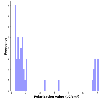
For this list, we were able to generate the canonical SMILEs and molecular formulas for all the compounds using PubChemKim et al. (2019) and OpenBabelO’Boyle et al. (2008, 2011) libraries. In turn, that allowed us to estimate the magnitudes of their spontaneous polarizations, which are also included in Table 3. The polarization magnitudes vary approximately between 1.238 and 7.098 $\mu$ C/cm². These values are obtained by averaging over 300 predictions by the model constructed using Dataset II to avoid any discrepancy (changes in magnitudes when the model is run multiple times) arising due to limited dataset size. A histogram plot of all predicted polarizations is shown in Fig. 5. As identified in the Table and Figure, there are nine compounds with predicted polarization of $\sim$ 7 $\mu$ C/cm², i.e., close in magnitude to experimental values reported for partially crystalline $\beta$ -PVDF.Nakhmanson et al. (2005); Meng et al. (2019) It is noteworthy that the quality of these predictions can be improved further if the compound structures are obtained directly from CSD, rather than created using PubChem and OpenBabel. Again, at this point, the list entries could be evaluated further on an individual basis, according to criteria (ii) and (iii) of Sec. I, to develop more accurate predictions of their propensity to exhibit ferroelectricity. However, since such activities involve performing DFT-based simulations and thus would be rather computationally expensive, they fall beyond the scope of this investigation. We point out that such computations (including more accurate estimation of spontaneous polarization exhibited by the polar phases and other related properties) are standard for DFT-based computational packages and could be easily carried out when necessary or desired.

III.3 A validation example

In this section we include an example showcasing how such an investigation, utilizing DFT to estimate the polar properties, can be conducted. The DFTHohenberg and Kohn (1964) calculations were performed using the Vienna ab initio simulation package (VASP)Kresse and Furthmüller (1996) within the projector-augmented-wave (PAW) scheme.Blöchl (1994) The Perdew-Burke-Ernzerh (PBE) functional was used to treat exchange and correlation interactionsPerdew et al. (1996). The cutoff energy was set at 520.0 eV and a $k$ -point mesh of 4 $\times$ 6 $\times$ 6 was used for the computations. All the structures were fully relaxed until all forces on all atoms are smaller than 0.001 eV/Å. Berry phase formalism was used to calculate spontaneous polarization $\mathbf{P}_{s}$ .Resta (1992)

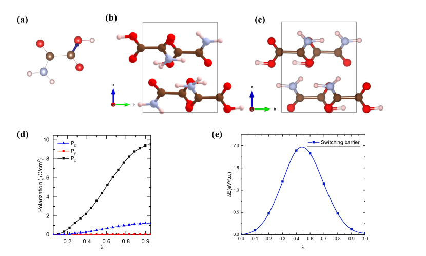
Here, the system of interest is oxamic acid (C₂H₃NO₃), that was predicted to have the polarization of 4.347 $\mu$ C/cm² by the ML model (see Table 3). A sketch of the (planar) C₂H₃NO₃ molecular unit is presented in Fig. 6(a). The direction of the unit net dipole moment is expected to be along the edge C atom bonded with an (-OH) functional group. This is because O is more electronegative than N present in the C-NH₂, located at the other edge of the molecular unit.

The bulk polar structureDugarte-Dugarte et al. (2019) is arranged of four molecular units, as shown in Fig. 6(b), and belongs to the $Cc$ space group. To estimate the spontaneous polarization for this system, the corresponding reference non-polar centrosymmetric structure was constructed.Capillas et al. (2011) The non-polar structure belongs to the $P2_{1}/c$ space group and is connected to the polar $Cc$ structure by a 180^∘ rotation of two of the four molecular units around the axis including the C–C bond, as shown in Fig. 6(c). A polar distortion parameter $\lambda$ is introduced to represent the transition path from the non-polar ( $\lambda$ = 0) to polar structure ( $\lambda$ = 1). The $x$ , $y$ , and $z$ components of the spontaneous polarization as a function of $\lambda$ are plotted in Fig. 6(d). The components, P_x, P_y, and P_z are along crystallographic axes $a$ , $b$ and $c$ , respectively. Although the difference in the ground-state energies for polar and non-polar phases are very close, the energy differences as obtained by performing a Nudge Elastic Band (NEB) computation suggests that the switching barrier (Fig. 6(e)) is high for the intermediate structures, $\sim$ 2 eV per molecular unit. Polarization components along $x$ (1.240 $\mu$ C/cm²) and $y$ ( $\sim$ 0 $\mu$ C/cm²) are minimal due to the canted arrangements of the molecular unit dipole moments, while $P_{z}$ is 9.510 $\mu$ C/cm². Although the DFT estimate for the system polarization is larger than the ML model prediction, it nonetheless falls remarkably close by the order of magnitude. A possible source of discrepancy may be in an overly simplified (cubic) generic structure of the polar phase created from the SMILE representation by the ML model, which is different from the actual structure shown in Fig. 6(b). Finally, we note that the polarization estimate for the oxamic acid molecular crystal ( $\sim$ 10 $\mu$ C/cm²) is a relatively large value for a polymer- or molecular-based ferroelectric, e.g., in comparison to typical polarizations exhibited by the PVDF family of materials, as well as some other compounds.Nakhmanson et al. (2005); Louis et al. (2018); Ghosh et al. (2018)

IV Conclusions

In conclusion, we have compiled datasets containing reports on molecular and polymer-based ferroelectric compounds from the available literature. Through various data analytics techniques, we have identified several descriptors that are critical for understanding polar properties of such systems and developed families of ML models that could predict the magnitude of spontaneous polarization in them. We have also applied data mining to shortlist potential organic ferroelectrics based on their polymorphism, symmetry and chemical makeup, and predicted the values of spontaneous polarization for them. Further investigations including checking the stability of the ground-state configurations and height of the energy barriers between structural phases can be easily accomplished and will significantly enhance the presented analysis, but are beyond the scope of this project as it is currently envisioned. Overall, the developed general prescription, employing both data-driven sampling techniques and ML models describing polar properties of organic crystals (but applicable to inorganic systems as well), helps us improve our understanding of mechanisms governing the emergence of such complex material functionalities, as well as identify potential candidates possessing such functionalities for further in-depth investigations.

Acknowledgements.

A.G. acknowledges the hospitality of Los Alamos National Laboratory, where this project was initialized. This work was supported by the U.S. DOE NNSA under Contract No. 89233218CNA000001 through the LANL Institute for Materials Science (IMS), and in part through the Center for Integrated Nanotechnologies, a U.S. DOE Office of Basic Energy Sciences user facility in partnership with the LANL Institutional Computing Program for computational resources. A.G. also acknowledges her current funding support from the U.S. DOE, Office of Science, Office of Basic Energy Sciences Data, Artificial Intelligence and Machine Learning at DOE Scientific User Facilities.

References

Choi et al. (2004) K. J. Choi, M. Biegalski, Y. Li, A. Sharan, J. Schubert, R. Uecker, P. Reiche, Y. Chen, X. Pan, V. Gopalan et al., Science, 2004, 306, 1005–1009.
Lee et al. (2005) H. N. Lee, H. M. Christen, M. F. Chisholm, C. M. Rouleau and D. H. Lowndes, Nature, 2005, 433, 395.
Lovinger (1983) A. J. Lovinger, Science, 1983, 220, 1115–1121.
Furukawa (1989) T. Furukawa, IEEE transactions on electrical insulation, 1989, 24, 375–394.
Kepler and Anderson (1992) R. G. Kepler and R. Anderson, Advances in physics, 1992, 41, 1–57.
Nalwa (1995) H. S. Nalwa, Ferroelectric polymers: chemistry: physics, and applications, CRC Press, 1995.
Eberle et al. (1996) G. Eberle, H. Schmidt and W. Eisenmenger, IEEE transactions on dielectrics and electrical insulation, 1996, 3, 624–646.
Samara (2001) G. A. Samara, Solid State Physics, 2001, 56, 239–458.
Horiuchi and Tokura (2008) S. Horiuchi and Y. Tokura, Nature Mater., 2008, 7, 357–366.
Heine and McConnell (1984) V. Heine and J. McConnell, J. Phys. C, 1984, 17, 1199.
Louis et al. (2018) L. Louis, K. C. Pitike, A. Ghosh, S. Poddar, S. Ducharme and S. M. Nakhmanson, J. Mater. Chem. C, 2018, 6, 1143–1152.
Ghosh et al. (2018) A. Ghosh, L. Louis, A. D. Asandei and S. Nakhmanson, Soft Matter, 2018, 14, 2484–2491.
Sattari et al. (2021) K. Sattari, Y. Xie and J. Lin, Soft Matter, 2021, –.
Lines and Glass (2001) M. E. Lines and A. M. Glass, Principles and applications of ferroelectrics and related materials, Oxford university press, 2001.
Ye et al. (2018) H.-Y. Ye, Y.-Y. Tang, P.-F. Li, W.-Q. Liao, J.-X. Gao, X.-N. Hua, H. Cai, P.-P. Shi, Y.-M. You and R.-G. Xiong, Science, 2018, 361, 151–155.
Groom et al. (2016) C. R. Groom, I. J. Bruno, M. P. Lightfoot and S. C. Ward, Acta Cryst. B, 2016, 72, 171–179.
Clark et al. (2006) A. M. Clark, P. Labute and M. Santavy, J. Chem. Inf. Model, 2006, 46, 1107–1123.
(18) Molecular Operating Environment, available from https://www.chemcomp.com/Products.htm.
Ward et al. (2018) L. Ward, A. Dunn, A. Faghaninia, N. E. Zimmermann, S. Bajaj, Q. Wang, J. Montoya, J. Chen, K. Bystrom, M. Dylla et al., Comput. Mater. Sci., 2018, 152, 60–69.
Ricci et al. (2020) F. Ricci, A. Dunn, A. Jain, G.-M. Rignanese and G. Hautier, Journal of Materials Chemistry A, 2020, 8, 17579–17594.
Ward et al. (2016) L. Ward, A. Agrawal, A. Choudhary and C. Wolverton, npj Computational Materials, 2016, 2, 1–7.
Pedregosa et al. (2011) F. Pedregosa, G. Varoquaux, A. Gramfort, V. Michel, B. Thirion, O. Grisel, M. Blondel, P. Prettenhofer, R. Weiss, V. Dubourg, J. Vanderplas, A. Passos, D. Cournapeau, M. Brucher, M. Perrot and E. Duchesnay, Journal of Machine Learning Research, 2011, 12, 2825–2830.
Ghosh et al. (2020) A. Ghosh, F. Ronning, S. M. Nakhmanson and J.-X. Zhu, Phys. Rev. Mater., 2020, 4, 064414.
Ghosh et al. (2019) A. Ghosh, L. Louis, K. K. Arora, B. C. Hancock, J. F. Krzyzaniak, P. Meenan, S. Nakhmanson and G. P. Wood, CrystEngComm, 2019, 21, 1215–1223.
Arthur et al. (2016) D. E. Arthur, A. Uzairu, P. Mamza, A. E. Stephen and G. Shallangwa, Chem. Data Collect., 2016, 5, 46–61.
Kaur et al. (2019) H. Kaur, H. S. Pannu and A. K. Malhi, ACM Computing Surveys, 2019, 52, 79.
Neal (2001) R. M. Neal, Stat Comput., 2001, 11, 125–139.
Chawla et al. (2002) N. V. Chawla, K. W. Bowyer, L. O. Hall and W. P. Kegelmeyer, Journal of artificial intelligence research, 2002, 16, 321–357.
Abdi and Williams (2010) H. Abdi and L. J. Williams, Wiley interdisciplinary reviews: computational statistics, 2010, 2, 433–459.
Scott (2018) D. W. Scott, in Kernel Density Estimation, American Cancer Society, 2018, pp. 1–7.
Kim et al. (2019) S. Kim, J. Chen, T. Cheng, A. Gindulyte, J. He, S. He, Q. Li, B. A. Shoemaker, P. A. Thiessen, B. Yu et al., Nucleic Acids Res., 2019, 47, D1102–D1109.
O’Boyle et al. (2008) N. M. O’Boyle, C. Morley and G. R. Hutchison, Chem. Cent. J., 2008, 2, 1–7.
O’Boyle et al. (2011) N. M. O’Boyle, M. Banck, C. A. James, C. Morley, T. Vandermeersch and G. R. Hutchison, J. Cheminformatics, 2011, 3, 33.
Nakhmanson et al. (2005) S. Nakhmanson, M. B. Nardelli and J. Bernholc, Phys. Rev. B, 2005, 72, 115210.
Meng et al. (2019) N. Meng, X. Ren, G. Santagiuliana, L. Ventura, H. Zhang, J. Wu, H. Yan, M. J. Reece and E. Bilotti, Nat. Commun., 2019, 1–9.
Hohenberg and Kohn (1964) P. Hohenberg and W. Kohn, Phys. Rev, 1964, 136, B864.
Kresse and Furthmüller (1996) G. Kresse and J. Furthmüller, Phys. Rev. B, 1996, 54, 11169.
Blöchl (1994) P. E. Blöchl, Phys. Rev. B, 1994, 50, 17953.
Perdew et al. (1996) J. P. Perdew, K. Burke and M. Ernzerhof, Phys. Rev. Lett., 1996, 77, 3865.
Resta (1992) R. Resta, Ferroelectrics, 1992, 136, 51–55.
Dugarte-Dugarte et al. (2019) A. J. Dugarte-Dugarte, J. van de Streek, A. M. dos Santos, L. L. Daemen, A. A. Puretzky, G. D. de Delgado and J. M. Delgado, J. Mol. Struct., 2019, 1177, 310–316.
Capillas et al. (2011) C. Capillas, E. S. Tasci, G. de la Flor, D. Orobengoa, J. M. Perez-Mato and M. I. Aroyo, 2011.

IV.1 Contributions

A.G. performed all computations and analysis and prepared all the figures. A.G., S.N. and J.-X.Z. developed the project idea. S.H., D.T., E.S. and H.T. participated in curation of experimental reports and code development. A.G. and S.N. wrote the paper with inputs from everyone.

IV.2 Conflicts of Interest

There are no conflicts of interest to declare.

IV.3 Additional Information

The author(s) declare no competing interests.