Geometrical aspect of susceptibility critical exponent

Abstract

Critical exponent $\gamma\succeq 1.1$ characterizes behavior of the mechanical susceptibility of a real fluid when temperature approaches the critical one. It results in zero Gaussian curvature of the local shape of the critical point on the thermodynamic equation of state surface, which imposes a new constraint upon the construction of the potential equation of state of the real fluid from the empirical data. All known empirical equations of state suffer from a weakness that the Gaussian curvature of the critical point is negative definite instead of zero.

Geometry plays important roles in thermodynamics. The modern version of thermodynamics can be reformulated in terms of contact geometry geom1 , and the so-called geometry of thermodynamics has been put forward which describes the space of thermodynamic parameters by the Riemannian metric geom2 ; geom3 ; geom4 . The influence of the curved space on the critical behavior of the two-dimensional Ising model is identified geom5 , and geometric critical exponents are definable in classical and quantum phase transitions geom6 . The new relationship between thermodynamical and geometry is always interesting, and we report a new requirement on the construction of the empirical equation of state (EoS) based on the differential geometry of the surfaces.

The elaboration of a better form of the empirical EoS best fitting the experimental data and also meeting the theoretical requirements have been an important issue for more than one century wei ; eos2 ; lw ; eos1 ; review1 ; review2 ; exp . For a real fluid, a theoretical problem which remains open for a long time is, in the close neighborhood of the critical point, what is the precise form of the EoS? For instance, it is well-known that both the van der Waals EoS and the general theory of the Landau theory of phase transitions, predicts the susceptibility critical exponent $\gamma=\gamma^{\prime}$ to be $1$, and all known empirical EoS fail to exactly reproduce the experimental values $\gamma=1.2\sim 1.3\gtrsim\gamma^{\prime}=1.1$ $\sim 1.2$ toda ; pathria . Recently, we conjecture that the Gaussian curvature of the local shape of the vapor-liquid critical point is zero liu2021 . In present paper, we prove that the conjecture is true, and secondly construct an fluid EoS which has $\gamma=\gamma^{\prime}=3$, which is compatible the zero Gaussian curvature of the vapor-liquid critical point.

The fluid of a pure substance belongs to the so-called $pVT$ system, which means that the EoS usually takes following form,

$$p=p(V,T),$$ (1)

where $p,V,T$ denote the pressure, volume and temperature, respectively. In general, this function has continuous first and second order derivatives at the critical point of which three parameters $\left(p_{c},V_{c},T_{c}\right)$ satisfy, in addition to the EoS (1),

$$\left(\frac{\partial p}{\partial V}\right)_{T_{c}}=0,\left(\frac{\partial^{2}p}{\partial V^{2}}\right)_{T_{c}}=0.$$ (2)

In present paper, we do not deal with piecewise or other discontinuous form of EoS (1).

To note that in geometry the EoS (1) can be viewed as a two-dimensional surface in the flat $pVT$ space, and its shape can be completely characterized by the mean and Gaussian curvature. docarmo It is then interesting to explore the local shape of the vapor-liquid critical point via these two curvatures. In calculation, the dimensionless EoS surface equation (1) must be used, in which all quantities $\left(p,V,T\right)$ are transformed into those referring to units $\left(p_{c},V_{c},T_{c}\right)$, or other units $\left(p^{\prime},V^{\prime},T^{\prime}\right)$ of specific states, respectively. The transformed form of EoS bears a resemblance to the law of corresponding states of the van der Waals EoS. The mean curvature $H$ and Gaussian curvature $K$ are, respectively, docarmo

$$H = \frac{\left(\frac{\partial^{2}p}{\partial V^{2}}\right)_{T}\left(\left(\frac{\partial p}{\partial T}\right)_{V}^{2}+1\right)+\left(\frac{\partial^{2}p}{\partial T^{2}}\right)_{V}\left(\left(\frac{\partial p}{\partial V}\right)_{T}^{2}+1\right)-2\left(\frac{\partial p}{\partial V}\right)_{T}\left(\frac{\partial p}{\partial T}\right)_{V}\left(\frac{\partial^{2}p}{\partial V\partial T}\right)}{2\left(\left(\frac{\partial p}{\partial V}\right)_{T}^{2}+\left(\frac{\partial p}{\partial T}\right)_{V}^{2}+1\right)^{3/2}},$$ (3)

$$K = \frac{\left(\frac{\partial^{2}p}{\partial V^{2}}\right)_{T}\left(\frac{\partial^{2}p}{\partial T^{2}}\right)_{V}-\left(\frac{\partial^{2}p}{\partial V\partial T}\right)^{2}}{\left(\left(\frac{\partial p}{\partial V}\right)_{T}^{2}+\left(\frac{\partial p}{\partial T}\right)_{V}^{2}+1\right)^{2}}.$$ (4)

At the critical point the conditions (2)  apply, we have the mean curvature $H_{C}$ and Gaussian curvature $K_{C}$, respectively,

$$H_{C}=\frac{\left(\frac{\partial^{2}p}{\partial T^{2}}\right)_{V}}{2\left(\left(\frac{\partial p}{\partial T}\right)_{V}^{2}+1\right)^{3/2}},K_{C}=-\frac{\left(\frac{\partial^{2}p}{\partial V\partial T}\right)^{2}}{\left(\left(\frac{\partial p}{\partial T}\right)_{V}^{2}+1\right)^{2}}.$$ (5)

The compressibility or a mechanical response function

$$\kappa_{T}\equiv-\frac{1}{V}\left(\frac{\partial V}{\partial p}\right)_{T}$$ (6)

corresponds to a susceptibility

$$\left(\frac{\partial p}{\partial V}\right)_{T}=-\frac{1}{V\kappa_{T}}.$$ (7)

Near the critical point, the experiments suggest, with $\gamma=\gamma^{\prime}\succeq 1.1$, toda ; pathria

$$\kappa_{T}\propto\left\{\begin{array}[]{cc}\left(T-T_{c}\right)^{-\gamma},&\left(T\rightarrow T_{c}+0\right)\\ \left(T_{c}-T\right)^{-\gamma^{\prime}},&\left(T\rightarrow T_{c}-0\right)\end{array}\right..$$ (8)

In consequence, we have,

$$\frac{\partial^{2}p}{\partial V\partial T}=-\frac{1}{V}\frac{\partial}{\partial T}\left(\frac{1}{\kappa_{T}}\right)\propto\left\{\begin{array}[]{cc}\left(T-T_{c}\right)^{\gamma-1},&\left(T\rightarrow T_{c}+0\right)\\ \left(T_{c}-T\right)^{\gamma^{\prime}-1},&\left(T\rightarrow T_{c}-0\right)\end{array}\right.=0,$$ (9)

which can be rewritten into, in terms of the Gaussian curvature from (5),

$$K_{C}=0.$$ (10)

Thus, for real fluids, the Gaussian curvature of local shape of the critical point of the EoS surface is zero.

In contrast, none of the known typical empirical EoS can reproduce $K_{C}=0$, whose results are listed in following Table I. In the last line of the Table I, the Shamsundar-Lienhard EoS review2 is special, for it is rather a principle than an explicit form of an equation. ”The shape of the (experimental data) figure tells us that a cubic-like equation must be of the form” review2 , and ”the advantage of this form is that it automatically satisfies critical point criteria, … .” review2 Though these empirical EoS in the Table I do not exhaust all possibilities, we are safe to say that $K_{C}=0$ is beyond the current form of the Landau theory of phase transitions for it predicts $\gamma=\gamma^{\prime}=1,$ thus $K_{C}\prec 0$. toda ; pathria

Table 1: Mean and Gaussian curvature of the critical points for empirical or semi-empirical EoS. Symbol $v$ denotes the molar volume, $a$ and $b$ are repulsive and attractive parameter respectively, and $y=b/4v$, and $a(T)$ depends on temperature as well as on other substance parameters wei ; exp . Only one typical value of the substance parameter in $a(T)$ is used in the calculations.

No	References	EoS	$H_{C}$	$K_{C}$	Year
1	van der Waals	$\frac{RT}{v-b}-\frac{a}{v^{2}}$	0	-0.125	1873
2	Dieterici	$\frac{RT}{v-b}\exp\left(-\frac{a}{vkT}\right)$	0.063	-0.04	1916
3	Redlich-Kwong	$\frac{RT}{v-b}-\frac{a}{T^{1/2}v(v+b)}$	-0.006	-0.065	1949
4	Thiele	$\frac{RT}{v}\frac{1+y+y^{2}}{\left(1-y\right)^{3}}-\frac{a}{v^{2}}$	0	-0.099	1963
5	Guggenheim	$\frac{RT}{v}\frac{1}{1-y^{4}}-\frac{a}{v^{2}}$	0	-0.101	1965
6	Carnahan-Starling	$\frac{RT}{v}\frac{1+y+y^{2}-y^{3}}{\left(1-y\right)^{3}}-\frac{a}{v^{2}}$	0	-0.099	1969
7	Soave	$\frac{RT}{v-b}-\frac{a\left(T\right)}{v(v+b)}$	-0.004	-0.045	1972
8	Peng-Robinson	$\frac{RT}{v-b}-\frac{a\left(T\right)}{v(v+b)+b(v-b)}$	-0.003	-0.058	1976
9	Shamsundar-Lienhard	$g(T)\left(1-\frac{\left(V-V_{l}\right)\left(V-V_{m}\right)\left(V-V_{g}\right)}{f(V,T)}\right)$	/	0	1993

Now we present an EoS with $K_{C}=0$. Our constructed EoS takes following form,

$$p=\frac{8T}{9\left(V-\frac{1}{3}\left(\frac{19}{3}-\frac{6}{V}+\frac{2}{V^{2}}\right)\right)}-\frac{3\left(3-\frac{3}{T}+\frac{1}{T^{2}}\right)}{V^{2}}$$ (11)

where $\left(p,V,T\right)$ are written in unit $\left(p_{c},V_{c},T_{c}\right)\left(=\left(1,1,1\right)\right)$. It can be considered a highly distorted version of law of corresponding state of the van der Waals equation. The isotherms given by this EoS (11) are plotted in Fig. 1. Below the critical temperature $T_{C}$, the isotherms explicitly exhibit van der Waals loops. Straightforward calculations show that both the mean and the Gaussian curvature at the critical point are zero, i.e., $H_{C}=K_{C}=0$, and also an symmetrical susceptibility critical exponent,

$$\gamma=3\text{ }(T\rightarrow T_{C}+0)\text{, and }\gamma^{\prime}=3\text{ }(T\rightarrow T_{C}-0).$$ (12)

It is quantitatively different from the susceptibility critical exponent for the real fluid. The origin of the difference may lie in that we use the continuous form of the EoS from which we have in fact attempted many times, which shall be explored in the future.

So, far, there are at least three requirements on the form of EoS for the real fluid. 1) In large volume limit, the EoS reproduces the ideal gas law. review2 2) At both ends of a vapor-liquid coexistence line, there are onset and outset value for volume for gas and liquid state, and also a coexisting pressure. review2 3) The Gaussian curvature of the critical point is zero. All these constraints directly come from experiments. There may be other constraints on the form of the EoS, which may arise from the theoretical requirements such as Maxwell area construction for van der Waals loop, review2 which must used case by case.

In summary, geometry not only offers better understanding and deeper insight into the mathematical structure of the thermodynamics, but also presents an accurate and convenient means to characterize various properties of thermodynamic states. We report that the local shape of the vapor-liquid critical point on thermodynamic surface has zero Gaussian curvature, which has long hidden in the susceptibility critical exponent $\gamma\succ 1$. It can be used to distinguish different empirical models, and to impose on the construction of the new EoS as well. A new form of the EoS capturing the essential feature of the vapor-liquid phase transition with $\gamma\succ 1$ is successfully elaborated, which is still quantitatively different from the susceptibility critical exponent for the real fluid.

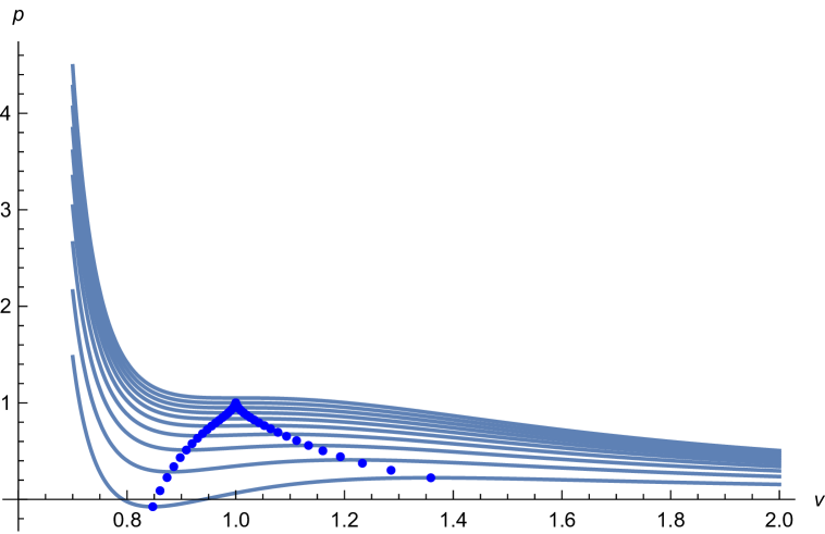
Figure 1: The isotherms (solid lines) with $T=0.60,0.65,0.70,...,1.05$ from undermost to upmost, and the spinodal curve (solid dots) for EoS (11). It clearly shows that the EoS captures the essential feature of the vapor-liquid phase transition.

- (1) R. Hermann, Geometry, Physics and Systems (New York: Dekker 1973).
- (2) F. Weinhold, Thermodynamics and geometry. Phys. Today 29(1976)23-30.
- (3) R. Gilmore, Length and curvature in the geometry of thermodynamics, Phys. Rev. A 30(1984)1994.
- (4) G. Ruppeiner, Riemannian geometry in thermodynamic fluctuation theory, Rev. Mod. Phys. 67(1995)605-659.
- (5) H. Shima and Y. Sakaniwa, Geometric effects on critical behaviours of the Ising model, J. Phys. A: Math. Gen. 39(2006)4921.
- (6) P. Kumar and T. Sarkar, Geometric critical exponents in classical and quantum phase transitions, Phys. Rev. E 90(2014)042145.
- (7) Y. S. Wei and R. J. Sadus, Equations of State for the Calculation of Fluid-Phase Equilibria, AIChE Journal, 46(2000)169
- (8) G. M. Kontogeorgis, R. Privat, and Jean-Noel Jaubert, Taking Another Look at the van der Waals EoS – Almost 150 Years Later. J. Chem. Eng. Data, 64(2019)4619-4637.
- (9) J. L. Lebowitz, E. M. Waisman, Statistical Mechanics of Simple Fluids: Beyond van Der Waals. Phys. Today, 33(1980)24-30.
- (10) R. C. Reid, J. M. Prausnitz and B. E. Poling, The Properties of Gases and Liquids (New York: McGraw-Hill, 1987).
- (11) J. H. Lienhard, N. Shamsundar and P.O. Biney, Spinodal Lines and Equations of State-a review, Nucl. Eng. Des. 95(1986)297-313.
- (12) N. Shamsundar and John H. Lienhard, Equations of state and spinodal lines a review, Nucl. Eng. Des. 141(1993)269-287.
- (13) A. Anderko, Cubic and generalized van der Waals equations, Experimental Thermodynamics, 5( 2000)75-126.
- (14) M. Toda, R. Kubo, N. Saito, Statistical Physics I: Equilibrium Statistical Mechanics, 2nd Ed., (Berlin: Sringer-Verlag, 2012).
- (15) R. K. Pathria, P. D. Beale, Statistical Mechanics, 3rd ed., (Oxford: Butterworth-Heinemann, 2011).
- (16) J. S. Yu, X. Zhou, J. F. Chen, W. K. Du, X. Wang and Q. H. Liu, Local Shape of the Vapor–Liquid Critical Point on the Thermodynamic Surface and the van der Waals EoS. Front. Phys. 9(2021)679083.
- (17) M. P. do Carmo, Differential Geometry of Curves and Surfaces (New York: Prentice-Hall, 1976).
- (18) J. D. Gunton and M. J. Buckingham, Condensation of the Ideal Bose Gas as a Cooperative Transition, Phys. Rev. 166(1968)152.