Functional Data Representation with Merge Trees
Abstract
In this paper we face the problem of representation of functional data with the tools of algebraic topology. We represent functions by means of merge trees and this representation is compared with that offered by persistence diagrams. We show that these two structures, although not equivalent, are both invariant under homeomorphic re-parametrizations of the functions they represent, thus allowing for a statistical analysis which is indifferent to functional misalignment. We employ a novel metric for merge trees and we prove some theoretical results related to its specific implementation when merge trees represent functions. To showcase the good properties of our topological approach to functional data analysis, we test it on the Aneurisk65 dataset replicating, from our different perspective, the supervised classification analysis which contributed to make this dataset a benchmark for methods dealing with misaligned functional data.
Keywords: functional data analysis, functional alignment, merge trees, tree edit distance, topological data analysis.
1 Introduction
Since the publication of the seminal books by Ramsay and Silverman (Ramsay and Silverman, 2005) and Ferraty and Vieu (Ferraty and Vieu, 2006), Functional Data Analysis (FDA) has become a staple of researchers dealing with data where each statistical unit is represented by the measurements of a real random variable observed on a grid of points belonging to a continuous, often one dimensional, domain In FDA these individual data are better represented as the sampled values of a function defined on and with values in Hence, at the onset of any particular functional data analysis stands the three-faceted problem of representation, described by: (1) the smoothing of the raw and discrete individual data to obtain a functional descriptor of each unit in the data set, (2) the identification of a suitable embedding space for the sample of functional data thus obtained and, finally, (3) the eventual alignment of these functional data consistently with the structure of the embedding space. As a reference benchmark of the typical FDA pipeline applied to a real world dataset, we take the paper by Sangalli et al. (2009b) where the first functional data analysis of the AneuRisk65 dataset is illustrated.
Smoothing is the first step of a functional data analysis. For each statistical unit, individual raw data come in the form of a discrete set of observations regarded as partial observations of a function. Smoothing is the process by means of which the analyst generates the individual functional object out of the raw data. This functional object will be the atom of the subsequent analysis, a point of a functional space whose structure is apt to sustain the statistical analysis required by the problem at hand. A common approach to obtain functional representations is to fit the data with a member of a finite dimensional functional space generated by some basis, for instance, splines or trigonometric polynomials. Signal-to-noise ratio and the degree of differentiability required for the functional representation, as well as the structure of the embedding space, drive the smoothing process. Functional representations interpolating the raw data are of no practical use when the analysis requires to consider functions and their derivatives or, for instance, the natural embedding space is Sobolev’s; see, for instance, Sangalli et al. (2009a) for a detailed analysis of the trade-off between goodness of fit and smoothness of the functional representation when dealing with the Aneurisk65 dataset.
Functional data express different types of variability (Vantini, 2009) which the analyst might want to decouple before carrying out the statistical analysis. Indeed the Aneurisk65 dataset is by now considered a benchmark for methods aimed at the identification of phase and amplitude variation (see the Special Section on Time Warpings and Phase Variation on the Electronic Journal of Statistics, Vol 8 (2), and references therein). In many applications phase variation captures ancillary non-informative variability which could alter the results of the analysis if not properly taken into account (Lavine and Workman, 2008; Marron et al., 2014). A common approach to this issue is to embed the functional data in an appropriate Hilbert space where equivalence classes are defined, based on a notion of alignment or registration, and then to look for the most suitable representative for any of these classes (Marron et al., 2015). Such approach evokes ideas from shape analysis (Dryden and Mardia, 1998) and pattern theory (Grenander, 1993), where configurations of landmark points are identified up to rigid transformations and global re-scalings. In close analogy with what has been done for curves (Michor et al., 2007; Srivastava et al., 2011b), functions defined on compact real intervals are aligned by means of warping functions mapping into another interval; that is, functional data are identified up to some re-parametrization. Different kinds of warping functions have been investigated: affine warpings are studied for instance in Sangalli et al. (2010) while more general diffeomorphic warpings have been introduced in Srivastava et al. (2011a). Once the best representatives are selected, the analysis is carried out on them leveraging the well behaved Hilbert structure of the embedding space. Classically, the optimal representatives are found by minimizing some loss criterion with carefully studied properties (Sangalli et al., 2014). This approach however has some limitations, arising from the fact that the metric structure of the embedding space might not be compatible with the equivalence classes collecting aligned functions (Yu et al., 2013). An alternative is to employ metrics directly defined on equivalence classes of functions such as the Fisher Rao metric, originally introduced for probability densities (Srivastava et al., 2007), which allows for the introduction of diffeomorphic warpings (Srivastava et al., 2011a). It must be pointed out that all these ways of dealing with the issue of ancillary phase variability encounter some serious challenges when the domain is not a compact real interval.
A different approach to the problem of phase variation is to capture the information content provided by a functional datum by means of a statistic which is insensitive to the function re-parametrization, but sufficient for the analysis. Algebraic topology can help since it provides tools for identifying information which is invariant to deformations of a given topological space (Hatcher, 2000). Topological Data Analysis (TDA) is a quite recent field in data analysis and consists of different methods and algorithms whose foundations rely on the theory developed by algebraic topology (Edelsbrunner and Harer, 2008). The main source of information collected by TDA algorithms are homology groups (see, for instance, Hatcher (2000)) with fields coefficients which, roughly speaking, count the number of holes (of different kinds) in a topological space. For instance zero dimensional holes are given by path connected components and one dimensional holes are given by classes of loops (up to continuous deformations) which cannot be shrunk to one point. One of the most interesting and effective ideas in TDA is that of persistent homology (Edelsbrunner et al., 2002): instead of fixing a topological space and extracting the homology groups from that space, a sequence of topological spaces is obtained along various pipelines, and the evolution of the homology groups is tracked along this sequence. The available pipelines are many, but the one which is most interesting for the purposes of this work is that concerning real valued functions. Let the domain be a topological space and consider a real valued function defined on One can associate to the sequence of topological spaces given by the sublevel sets , with ranging in The evolution of the connected components along is thus analysed for the purpose of generating a topological representation of
In this work, we consider specific topological representations of constructed along this general scheme and we show that they are invariant with respect to homeomorphic warpings of the domain Moreover, these representations are also able to separate big shape features of from small oscillations; the overall shape of the function captured by the topological representations we will deal with is unaffected by the presence of smaller oscillations, which are captured as well, but separately. These two properties make the TDA approach pursued in this manuscript a candidate for the representation of functional data, indeed a robust competitor able to deal in a natural way with phase variation and insensitive to the fine tuning of the preliminary smoothing phase, since functional features likely generated by overfitted representations are easily identified as ancillary in the subsequent topological representation.
To allow for the statistical analysis of functional data summarised by their topological representations, we need to embed the latter in a metric space. The choice of persistence diagrams (PD) (Cohen-Steiner et al., 2007) as summaries obtained through persistent homology drives many successful applications (Xia et al., 2018; Bhattacharya et al., 2015; Pokorny et al., 2016; Chung et al., 2009; Wang et al., 2018; Kramár et al., 2013), although other topological summaries are in fact known in the literature (Bubenik, 2015; Adams et al., 2017; Chazal et al., 2015). In this work we exploit a topological alternative – not equivalent – to a persistence diagram, called merge tree. Merge trees representations of functions are not new (Morozov and Weber, 2013) and are obtained as a particular case of Reeb Graphs (Shinagawa et al., 1991; Biasotti et al., 2008). Different frameworks have been proposed to work with merge trees (Beketayev et al., 2014; Morozov et al., 2013), mainly defining a suitable metric structure to compare them (Gasparovic et al., 2019; Touli, 2020). However all such metrics have a very high computational cost, causing a lack of examples and applications even when approximation algorithms are available (Touli and Wang, 2019), or they require complex workarounds to be effectively used (Sridharamurthy et al., 2020). We employ the metric for merge trees introduced in Pegoraro (2021b), which is based on an edit distance presented in Pegoraro (2023) for more general graphs, and showing that its computational complexity is reasonable when the trees involved are not too large. When working with representations of data, it is fundamental to study the behaviour of the operator which maps the single datum into the chosen representation to assess which kind of information is transferred from the initial data to the space of representations. For this reason we develop a new theoretical analysis on the stability/continuity of merge trees with respect to perturbations of the original functions. We also carry out examples to showcase differences between merge trees and persistence diagrams of functions. Having devoted the initial sections of the paper to the understanding of the behaviour of these topological tools, we finally tackle, with our TDA approach, the benchmark functional classification case study detailed in Sangalli et al. (2009b).
Outline
The paper is organized as follows. In Section 2, we introduce the merge tree representation of a function. In Section 3 we briefly recall the definition of persistence diagrams in order to draw, in Section 4, some comparison between them and merge trees, before proving the invariance property which holds true for both topological representations. In Section 5 we present the metric structure for the space of merge trees which is used in the examples and in the final case study. In Section 6 we investigate the continuity properties of the operator which assigns to a function its merge tree, with respect to the aforementioned metric. Lastly, in Section 7, we tackle the functional data classification problem explored in Sangalli et al. (2009b) and we compare their results with those obtained following the TDA approach we advocate in this paper. We finally conclude the manuscript with a discussion, in Section 8, which points out some ideas pertaining to our topological approach to functional data analysis.
Section A of the supplementary material develops a detailed discussion on some topological issues touched upon only briefly in the main manuscript. Then, in Section B, we propose some in silico examples to further illustrate differences and similarities between persistence diagrams and merge trees together with one example on the use of the pruning operator. Section C contains some considerations on the consequences of Section 6 in the particular case of spline spaces. Section D contains an unsupervised approach to the Aneurisk65 data set, which provides an additional point of view on the information captured by merge trees. Further insights on the topic are presented in Section E, where merge trees are interpreted via some functional statistics. Section F contains additional figures and tables which were not included in the manuscript because of space constraints and which can help the reader in navigating through the manuscript. Lastly, Section G collects the proofs of the results of the paper.

2 Merge Trees of Functions
In this section we define the merge tree representation of a function. Merge trees are an already established tool in topology and, to some extent, also in statistics since dendrograms can be regarded as merge trees. Nevertheless, we are going to spend a few lines to define them, in accordance with the framework of Pegoraro (2021b), which differs from the classical one, found, for instance, in Morozov and Weber (2013). Roughly speaking, the pipeline to obtain a merge tree is the following: we transform the given function into a sequence of nested subsets and then we track the topological changes along this sequence. Such information is then turned into a tree.
The details are described in the following subsections.
2.1 Sublevel Sets
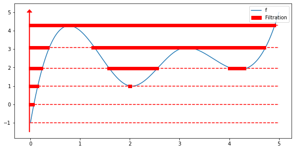
Consider a function , with being any topological space. We call sublevel set at height , the set . The key property of the family is that such subsets are nested: if then . Note that the sequence is fully determined by the shape of the function ; see Figure 1(a). In fact, for , hence no information carried by is lost by its representation .
2.2 Path Connected Components
A topological space is path connected if for every couple of points there is a continuous curve such that and . The biggest path connected subsets contained in a topological space are called path-connected components.
We call the set of the path connected components of . If is a continuous function, consider the function defined as follows: It is well known that is a (covariant) functor (Mac Lane, 1998) and thus satisfies a number of properties. Among them, we emphasize the following: for two continuous functions that can be composed into the function , it is true that .
Path connected components are the source of information we want to track along the family For let be the set of the path-connected components of . Let ; then we have: such that for all .
2.3 Tree Structures, Critical Values and Topological Changes
Coherently with Pegoraro (2021b), we now define what we mean with tree and with merge tree.
Definition 1
A tree structure is given by a set of vertices and a set of edges which form a connected rooted acyclic graph. We indicate the root of the tree with . We say that is finite if is finite. The order of a vertex of is the number of edges which have that vertex as one of the extremes. Any vertex with an edge connecting it to the root is its child and the root is its father: this is the first step of a recursion which defines the father and children relationship for all vertices in The vertices with no children are called leaves or taxa. The relation generates a partial order on . The edges in are identified in the form of ordered couples with . A subtree of a vertex is the tree structure whose set of vertices is .
Definition 2 (Gasparovic et al. (2019), Pegoraro (2021b))
A finite tree structure T such that is of order , coupled with a monotone increasing height function with and if , is called merge tree.
Let us now see how we can represent a real valued function by means of a merge tree. To do so, we need to make some key assumptions, known in the literature to be apt to produce constructible objects (De Silva et al., 2016; Patel, 2018; Curry et al., 2022).
Assumption 1
Given a family of topological spaces with , , we assume the existence of a finite collection of real numbers , called critical set, such that, given if or , then is bijective. The values are called critical values. As in Pegoraro (2021b) we always consider a minimal set of critical values, that is, the smallest possible set of critical values. With this condition, for any critical value there is some constant such that for all , is not bijective. Moreover, we assume that for every is finite. A function such that its sublevel set filtration satisfies the above set of hypotheses is called tame (Chazal et al., 2016). Lastly, we also assume that is path connected.
Together with the tameness of and the path-connectedness of we make an extra and simplifying regularity assumption - not needed, for the general construction of a merge tree - which implies a strong property of the critical values of the sublevel set filtration of This assumption can in fact be weakened, at the cost of some non trivial topological details (for more details see also Pegoraro (2021b)). For the sake of clarity, we defer the discussion about this issue to Section A.
Let be a critical value of the sublevel set filtration of Let be such that and . The properties of imply that . Due to the minimality condition stated in 1 we know that is not bijective.
Assumption 2
We assume that the sublevel set filtration of is regular: that is, for every critical value of there is a such that, for all , the map is bijective.
When is bijective, we say that the topological changes happen at the critical value , as opposed to across . Hence we are assuming that all the topological changes of happen at the critical values.
Remark 1
From the topological point of view, what lies behind the requirement that the topological changes happen at critical values is the following. Let and for . By construction, and for all . Which means . If is path connected then and we can’t have another path connected component such that .
All of this implies that, for - i.e. is injective at and . So, if for every path connected component the set is non empty and path connected, then is bijective. However, in general, need not be non empty and path connected!
Remark 2
Two notable cases where the topological changes happen at critical values are that of a continuous function defined on a connected compact subset of and that of an defined on a finite graph.
Indeed, let be continuous and be a compact interval. Then, for all is closed, since is continuous, and its path connected components are compact intervals of the form . Each path connected component is thus a convex set and any intersection of the form is non-empty and convex; that is, is non empty and path connected. Thus, for continuous functions , with being a compact interval, the topological changes always happen at critical values.
Consider now the discrete setting of a finite graph , with vertices and edges , such that the sublevel set filtration is well defined (i.e. for any edge connecting two vertices and , we have ). Let be the image of . Then, for all . This implies that all topological changes happen at critical values.
In light of 2, we point out that all the functions considered in the present work, those illustrated in the examples or those pertaining to the case study described in Section 7, do satisfy our 2, and the same is true for all numerical implementations.
The heuristic idea behind the construction of the merge tree representation of is that, since along the sequence the path-connected components of can only arise, merge with others (at critical values), or stay the same, it is natural to represent this merging structure with a tree structure However, this tree would not encode the critical values of hence we enrich it by defining a monotone increasing height function encoding them.
The tree structure and the height function are built along the following rules, in a recursive fashion starting from an empty set of vertices and an empty set of edges . We simultaneously add points and edges to and define on the newly added vertices. From now on, we indicate with the cardinality of a finite set
Considering the critical values in increasing order:
-
•
for the critical value add to a leaf , with height , for every element ;
-
•
for with , for every such that , add to a leaf with height ;
-
•
for with , if , with and distinct path connected components in , add a vertex with height , and add edges so that we connect the newly added vertex with each of the previously added vertices :
The last merging happens at height and, since is path connected, at height there is only one point . Thus we can add a vertex and an edge with to obtain a merge tree. The reader can look at Figure 1(b) for a first example of a merge tree associated to a function. The height function is given by the dotted red lines. We can appreciate that the merge tree of is heavily dependent on the shape of , in particular on the displacement of its maxima and minima.
2.4 Isomorphism classes
Before continuing we must decide on the topological information which we regard as equivalent. In other words, which merge trees we want to distinguish and which we do not. This step is essential and decisive to tackle the phase variation problem presented in the introduction: to select information that is insensitive to some kind of transformation amounts to defining classes of functions which are represented by the same tree. As in Pegoraro (2021b) and Pegoraro (2021a), we opt for a very general solution: we remove from the vertices of the tree any information regarding the connected components they are associated to, for instance, size, shape, position, the actual points contained etc..
Definition 3
Two tree structures and are isomorphic if there exists a bijection inducing a bijection between the edges sets and : . Such is an isomorphism of tree structures.
Definition 4
Two merge trees and are isomorphic if and are isomorphic as tree structures and the isomorphism is such that . Such is an isomorphism of merge trees.
The rationale behind 4, and the equivalence classes of isomorphic merge trees it generates, is analogous to that moving the introduction of persistence diagrams, where no specific information about individual path connected components is retained (see Section 3 for more details). Moreover, 4 does not require any additional structure for the space Other choices are possible; for instance, if the path connected components of could be given a natural ordering.
2.5 Height and Weight Functions
A final step is needed to complete the specific representation of merge trees needed for making use of the metric defined in Pegoraro (2021a). The height function of a generic merge tree takes values in but this is not an editable space, according to the definition in Pegoraro (2021b), which we report here.
Definition 5
Let be a set endowed with a metric and an associative operation with zero element Then is said to be an editable space if the following two properties are both satisfied:
-
(P1)
the map is a map of monoids between and that is: for all
-
(P2)
is invariant, that is: for all
Note that, whereas is not editable because , is editable.
We thus complement the merge tree with a transformation of the height function a weight function defined on whose image is a subset of the editable space . To do so, as in Pegoraro (2021a), we employ a truncation strategy which takes care of the edge which goes at infinity. Such strategy relies on the following assumption.
Assumption 3
We assume the existence of a universal constant bounding above all the functions for which we will adopt a merge tree representation.
In Pegoraro (2021a) it is shown that all the upcoming steps in the construction of the specific merge trees considered in this paper, do not depend on in the sense that with any we would obtain the same results. We spend some more words on this issue in the following 5.
Given a merge tree , as a first step we define the function as for all and . Then for every vertex we consider the unique edge between and its father and we define the weight function also codes the weight of the edge , via the rule , which identifies the set of edges with vertices in . Note that, because of 3, there is a one-to-one correspondence between and Finally, the monotonicity of and 3 guarantee that for all See Figure 13 for a visual example.
The height function introduced in 2 turns out to be quite natural for the definition of a merge tree, but from now on along with the height function we also employ the induced weight functions .
3 Persistence Diagrams
Persistence diagrams are arguably among the most well known tools of TDA; for a detailed survey see, for instance, (Edelsbrunner and Harer, 2008). We here briefly introduce persistence diagrams since in the following sections we use them to draw comparisons with merge trees.
Loosely speaking a persistence diagram is a collection of points in the first quadrant of , with and such that: is the corresponding to the first appearance of an homology class in (birth), while is the where the same class merges with a different class appeared before (death). Homology classes are a generalization of path-connected components to “holes in higher dimension”; path-connected components can be seen as zero dimensional holes. For more details see Hatcher (2000).
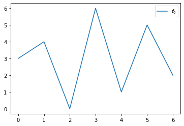

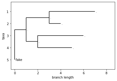
In this work we focus on persistence diagrams associated to path-connected components, since we want to compare them with the merge trees introduced in the previous section. Given a function we associate to the zero dimensional persistence diagram () of the sequence of sublevel sets . We highlight that, in such representation, there is no information about which path-connected component merges with which; in fact a component represented by the point , at height could merge with any of the earlier born and still alive components. Of course this collection of points still depends on the shape of the function and in particular depends on its amplitude and the number of its oscillations. See Figure 2. Note that, while for merge trees one needs to be careful and consider appropriate isomorphism classes so that the representation does not depend, for instance, on the names chosen for the vertices (that is, the set ), this issue does not appear with persistence diagrams. Topological features are represented as points in the plane, without labels or other kinds of set-dependent information. Thus, two persistence diagrams are isomorphic if and only if they are made of the same set of points.
4 Properties
In this section we state the main invariance result anticipated in the introduction and we also point out a few differences between persistence diagrams and merge trees.
Proposition 1 (Invariance)
The (isomorphism class of the) merge tree and the persistence diagram representations of the function , are both invariant under homeomorphic re-parametrization of .
Remark 3
As an immediate consequence of 1 we obtain that, if the functions and can be aligned by means of an homeomorphism, that is if being an homeomorphism, then their associated merge trees and are isomorphic and the same holds for and .
In other words, we can warp, deform, move the domain of a function by means of any homeomorphism, and this will have no effect on its associated PD or merge tree. As a consequence, if each element of a sample of functions is represented by its merge tree, or by its persistence diagram, one can carry out the statistical analysis without worrying about possible misalignements, that is without first singling out, for each function of the sample, the specific warping function, identified by an homeomorphism, which decouples its phase and amplitude variabilities.
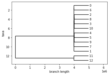
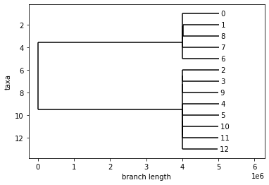
Despite sharing this important invariance property, a persistence diagram and a merge tree are not equivalent representations of a function. Indeed, persistence diagrams do not record information about the merging components: as already mentioned, the death of a path connected component could be caused by its merging with any other alive component at death-time. This implies that, for a given persistence diagram PD, there might be more than one merge tree associated to the diagram: the birth and death of the path connected components of each merge tree coincide with those of the PD, but the merging structure is different from merge tree to merge tree (Kanari et al., 2020; Curry et al., 2021; Pegoraro, 2021b; Curry et al., 2022; Elkin and Kurlin, 2020; Smith and Kurlin, 2022). In particular, the works of Kanari et al. (2020) and of Curry et al. (2021) formally address this point, by providing explicit formulas for the tree realization number: the number of trees associated to the same persistence diagram. This number can be very high, being if is the number of points in the diagram, for certain configurations of the persistent diagram. This is the case, for instance, with hierarchical clustering dendrograms with leaves: all leaves are born at height , and so, at the first merging point, each of the leaves can merge with any of the remaining ones. At the following merging step we have clusters and each one of them can merge with the other and so on. Thus, depending on the structure of the persistence diagram representing a function , the associated merge tree could contain much more information regarding from a different perspective, merge trees can discriminate between functions which are indistinguishable for persistent diagrams. To see some easy examples of how merge trees capture also the local merging structure of the components which persistent diagrams cannot distinguish, see Figure 14 and Section B of the supplementary material. Moreover, with the next proposition we formally state that the information contained in the persistence diagram of a function can be completely retrieved from the merge tree representing . The previous part of this paragraph clearly indicates that the converse need not be true, as also shown in Figure 14.
Proposition 2
For all , the associated in dimension can be obtained by the associated merge tree
Thus, if two functions induce isomorphic merge trees, they also have the same persistence diagrams. Further details and insights on the differences between PDs and merge trees can be found in Section B of the supplementary material.
5 Metrics
We want to analyze sets of functions using merge trees and PDs, exploiting metrics which have already been defined respectively in Pegoraro (2021b) and in Cohen-Steiner et al. (2010). Here we quickly present such metrics, with a special focus on the metric for merge trees, since we use it to develop novel stability results in the next sections.
5.1 Metrics for Persistence Diagrams
The space of persistence diagrams can be given a metric structure by means of a family of metrics which derives from Wasserstein distances for bivariate distributions.
Given two diagrams and , the expression of such metrics is the following:
where and ranges over the functions partially matching points between diagrams and , and matching the remaining points of both diagrams with the line on the plane (for details see Cohen-Steiner et al. (2007)). In other words we measure the distances between the points of the two diagrams, pairing each point of a diagram either with a point on the other diagram, or with a point on . Each point can be matched once and only once. The minimal cost of such matching provides the distance.
5.2 The Metric for Merge Trees
The metric for tree-like objects defined in Pegoraro (2021b) and then adapted to merge trees in Pegoraro (2021a) is based on edit distances (Bille, 2005; Hong et al., 2017): they allow for modifications of a starting object, each with its own cost, to obtain a second object. Merge trees equipped with their weight function as defined in Section 2.5, fit into this framework; hence the space of merge trees can be endowed with a metric based on an edit distance and called in the following.
The distance is very different from previously defined edit distances, since it is specifically designed for comparing topological summaries, roughly meaning that all points which are topologically irrelevant can be eliminated by a merge tree without paying any cost. To make things more formal we here introduce the edits, as defined in Pegoraro (2021a).
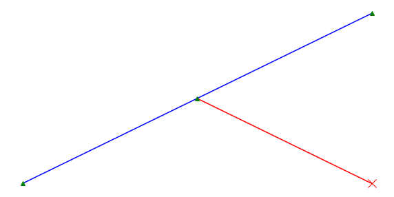
The edits are the followings and can be used to modify any edge of a merge tree, or equivalently its lower vertex :
-
•
shrinking an edge means changing the weight value of the edge with a new positive value. The inverse of this transformation is the shrinking which restores the original edge weight.
-
•
Deleting an edge results into a new tree, with the same vertices apart from (the lower one), and with the father of the deleted vertex which gains all of its children. With a slight abuse of language, we might also refer to this edit as the deletion of the vertex , which indeed means deleting the edge between and its father.
The inverse of deletion is the insertion of an edge along with its child vertex. We can insert an edge at a vertex specifying the child of and its children (that can be either none or any portion of the children of ) and the weight of the edge.
-
•
Lastly, we can eliminate an order two vertex , that is a father with an only child, connecting the two adjacent edges which arrive and depart from The weight of the resulting edge is the sum of the weights of the joined edges. This transformation is the ghosting of the vertex . Its inverse transformation is called the splitting of an edge.
Remark 4
Edit operations are not globally defined as operators mapping merge trees into merge trees. They are defined on the individual tree. Similarly, their inverse is not the inverse in the sense of operators, but it indicates that any time we travel from a tree to a tree by making a sequence of edits, we can also travel the inverse path going from to and restore the original tree.
The costs of the edit operations are defined as follows:
-
•
the cost of shrinking an edge is equal to the absolute value of the difference of the two weights;
-
•
for any deletion/insertion, the cost is equal to the weight of the edge deleted/inserted;
-
•
the cost of ghosting is zero.
Given a tree we can edit it, thus obtaining another tree, on which we can apply a new edit to obtain a third tree and so on. Any finite composition of edits is called an edit path. The cost of an edit path is the sum of the costs of its edit operations. Putting all the pieces together, we can define the edit distance as:
where indicates the set of edit paths which start in and end in .
Remark 5
The results in Pegoraro (2021a) show that the metric does not depend on the value of used in the truncation process and introduced with Assumption 3. To be sure, if, after having fixed to analyze a set of merge trees , we add to the set a new merge tree corresponding to a function which is not bounded above by , we proceed by fixing a novel bounding and all the other functions represented in the set , and compute , for all after truncating all merge trees in at height This won’t affect the distances between merge trees in computed before the addition of when the truncation constant was , since the metric is the same for such merge trees. Thus 3 is in some sense unnecessary, since we do not need to fix uniformly on our data set but only in a pairwise fashion. However for our applications such assumption is never violated, so we can assume it and avoid some formal complications arising from having to fix for every couple of functions.
5.2.1 Order Two Vertices
The null cost of ghosting guarantees that order vertices are completely irrelevant when computing the cost of an edit path.
Definition 6
If there is an edit path from the tree to the tree consisting only of ghosting or splitting edits, we say that the two trees are equal up to order vertices. By definition, the length of the edit path starting in and ending in is equal to .
In Pegoraro (2021b) it is proved that is a metric on the space of merge trees, identified up to order vertices. As explained in Pegoraro (2021b), the fact that order vertices are irrelevant is precisely what makes the metric suitable for comparing merge trees and is fundamental to obtain the results in Section 6.
6 Pruning & Stability
As stated in the introduction of the paper, any time we use a data representation – or we further transform a representation – it is important to understand and explore the properties of the operators involved. In particular, in this section we establish some continuity properties for the operator , which maps a function to its merge tree. Conditional on the topology endowing the functional space where the function is embedded, these properties dictate how the variability between functions is captured by the variability between their merge tree representations.
1 implies that the merge tree representation of a function is unaffected by a large class of warpings of its domain, which would strongly perturb if it was embedded, for instance, in an space, with . As an example, if is bounded with compact support, shrinking by setting with , produces no effect on the merge tree representation of since , while the -norm of goes to zero.
It might therefore be more natural to study the behavior of endowing the space of functions with the topology of pointwise convergence, which captures pointwise closeness between functions. This topology, available for any domain , has also the advantage of showing the effect of pointwise noise on merge tree representations.
6.1 Pruning
We know that, given , the merge tree will mostly depend on the critical points of : as the number of spikes of grows, also the size of the tree grows, while the weights of its branches grow with the height of the spikes. Similarly, if two functions are pointwise close, we can say that the shape of the functions is the same up to spikes of height . Each such spike would cause the birth of a leaf whose branch is shorter than ; the trees must therefore be similar up to branches of weight . These considerations move the idea of pruning, which consists of removing unessential edges from a tree.
Given a merge tree without order vertices, we want to delete the small weight leaves, that is those whose weight is smaller than or equal to a given fixed threshold. However, if two or more small weight leaves are siblings, we only need to remove that of smallest weight, or one of the leaves chosen at random if they have the same weight, and then ghost its father if it becomes an order vertex. To give a formal description of this procedure we resort to recursion as follows. Given and a merge tree , define the following 1-step process:
-
()
Take a leaf such that is minimal among all leaves; if two or more leaves have minimal weight, choose at random among them. If delete and ghost its father if it becomes an order vertex after removing .
For a given function we set the merge tree representing and we apply operation () to obtain . On the result we apply again () obtaining and, for we proceed iteratively until we reach the fixed point of the sequence Note that the fixed point is surely reached in a finite time since the number of leaves of each tree in the sequence is finite and non increasing along the sequence.
Remark 6
Applying to a merge tree representing a function is equivalent to removing a point with persistence smaller than that is from the persistence diagram representing . In fact a leaf such that is minimal, represents a connected component which, at height , meets another component which is born “earlier”, and so dies at such height. Its persistence is thus .
We can thus define the pruning operator such that is the tree obtained by pruning with threshold . See Figure 15 for a visual example. Notice that is idempotent, that is . On top of that, by construction, we have that .
Remark 7
is not a continuous operator. Consider formed by just one edge with weight ; take and consider , with the same tree structure as but made by one edge of weight . Now, and . If we let , then .
6 makes more evident and interpretable what happens at a topological level when pruning a merge tree representing a function . With the following results, instead, we want to interpret the pruning procedure at a functional level, showing that it amounts to removing only a small spike of at the time, whilst preserving the spikes of with amplitude larger than the fixed threshold.
Lemma 1
Let be a continuous function with being a topological space and let Then for every
Proposition 3
Let be a path connected and locally path connected topological space and let be a continuous tame function. Consider the merge tree associated to . Let and set . Then, there exist a function continuous and tame such that for all and is isomorphic to up to deleting and - eventually - ghosting .
Corollary 1
Given merge tree of a continuous tame function with being a path connected and locally path connected topological space, for every there is tame and continuous such that and is isomorphic to .
For what has been said up to now, the operator can be considered as a supplementary smoothing operator. We fix some threshold which we think captures meaningful shape changes in a function and then, consistently, we remove what is deemed to be noise or nuisance - due, for instance, to overfitting in its smoothing pre-processing - from the representation, obtaining a more regular merge tree. This has also the effect of greatly decreasing the number of leaves of the tree, a fact that is important from the computational perspective.
In Section B.4 we carry out a complete example to showcase the effectiveness of pruning when working with a function presenting some undesirable minor oscillations, along with a possible pipeline to select the pruning threshold.
6.2 Stability
Now we study the case of two merge trees and representing functions and which are pointwise close.
The main result of this section is the following.
Theorem 1
Let be tame functions defined on a path connected topological space and such that
Let and be the merge trees associated to and respectively and let and be the cardinalities of and .
Then, there exists an edit path such that for
1 states that if two functions are pointwise close, then we can turn the merge tree associated to the first function into the merge tree associated to the second function using at most one edit per vertex, and each edit has a small cost. Note, however, that if the two functions have a very high number of oscillations, the distance between their merge trees could still be large. Indeed if with we are not guaranteed that . 1 however implies that, if the cardinalities are bounded, then indeed goes to
Problems could then arise when we expect a possibly unbound number of informative spikes, that is spikes which should not be removed by pruning. In this case, however, the computational cost of the metric would also be prohibitive due to the high number of leaves in the trees; indeed this supports the claim that the only practical limitation to the use of the metric is given by its computational cost.
7 Case Study
We now run a comparative analysis of the real world Aneurisk65 dataset. This dataset – and the clinical problem for which it was generated and studied – was first described in Sangalli et al. (2009b), but it has since become a benchmark for the assessment of FDA methods aimed at the supervised or unsupervised classification of misaligned functional data (see, for instance, the special issue of the Electronic Journal of Statistics dedicated to phase and amplitude variability - year 2014, volume 8). We then repeat the classification exercise illustrated in Sangalli et al. (2009b) with the double scope of comparing merge trees and persistent diagrams when used as representations of the Aneurisk65 misaligned functional data, and of evaluating the performance of these representations for classification purposes when compared with the results obtained with the more traditional FDA approach followed by Sangalli et al. (2009b).
7.1 Dataset
The data of the Aneurisk65 dataset were generated by the AneuRisk Project, a multidisciplinary research aimed at investigating the role of vessel morphology, blood fluid dynamics, and biomechanical properties of the vascular wall, on the pathogenesis of cerebral aneurysms. The project gathered together researchers of different scientific fields, ranging from neurosurgery and neuroradiology to statistics, numerical analysis and bio-engineering. For a detailed description of the project scope and aims as well as the results it obtained see its web page (https://statistics.mox.polimi.it/aneurisk) and the list of publications cited therein.
Since the main aim of the project was to discover and study possible relationships between the morphology of the inner carotid artery (ICA) and the presence and location of cerebral aneurysms, a set of three-dimensional angiographic images was taken as part of an observational study involving 65 patients suspected of being affected by cerebral aneurysms and selected by the neuroradiologist of Ospedale Niguarda, Milano. These 3D images where then processed to produce 3D geometrical reconstructions of the inner carotid arteries for the 65 patients. In particular, these image reconstructions allowed to extract, for the observed ICA of each patient, its centerline “raw” curve, defined as the curve connecting the centres of the maximal spheres inscribed in the vessel, along with the values of the radius of such spheres. A detailed description of the pipeline followed to identify the vessel geometries expressed by the AneuRisk65 functional data can be found in Sangalli et al. (2014).
Different difficulties arise when dealing with this data. First, as detailed in Sangalli et al. (2009a), to properly capture information affecting the local hemodynamics of the vessels, the curvature of the centerline must be obtained in a sensible way. Retrieving the salient features of the centerline and of its derivatives is a delicate operation, which is heavily affected by measurement errors and reconstruction errors, due to the complex pipeline involved. Consequently the “raw” curves appear to be very wiggly and it is not obvious how to produce reasonable smooth representations. At the same time the 3D volume captured by the angiography varies from patient to patient. This is due to many factors, such as: the position of the head with respect to the instrument, which in turns depends on the suspected position of the aneurysm, the disposition of the vessels inside the head of the patient, the size of the patient. As shown by Figure 16 in the supplementary material, one can recognize these differences even by visual inspection: for instance, in Figure 16(a) and Figure 16(i) we see a longer portion of the ICA than in Figure 16(e). Therefore the reconstructed ICAs cannot be compared directly: we need methods that take into account that the centerlines are not embedded in in the same way, and that we cannot expect potentially interesting features to appear in exactly the same spots along the centerline. This is the typical situation where one should resort to alignment.
Hence, this dataset is paradigmatic of the three-faceted representation problem highlighted in the introduction; data smoothing, embedding, and alignment present difficult challenges, which propelled a number of original works in FDA.
The AneuRisk65 data have been already partially processed; in particular centerlines have been smoothed following the free-knot regression spline procedure described in Sangalli et al. (2009a), and their curvatures were thus obtained after computing the first two derivatives of the smoothed curves. The data relative to the radius of the blood vessel, instead, although measured on a very fine grid of points along the centerline, is still in its raw format. Hence the AneuRisk65 data also allow us to compare the behaviour of tree representations on smoothed data and on raw data.
7.2 Analysis
Patients represented in the AneuRisk65 dataset are organized in three groups: the Upper group (U) collects patients with an aneurysm in the Willis circle at or after the terminal bifurcation of the ICA, the Lower group (L) gathers patients with an aneurysm on the ICA before its terminal bifurcation, and finally the patients in the None group (N) do not have a cerebral aneurysm. Our main goal is supervised classification with the aim to develop a classifier able to discriminate membership to the group against membership to the group based on the geometric features of the ICA. In the supplementary material, we complement this supervised analysis with a descriptive analysis of the merge trees, aggregated according to their group membership, and an unsupervised exercise which aims at clustering patients solely on the basis of the similarity of geometric features of their ICA, thus recovering a clear structure between the groups listed above and providing further support to the discriminating power of the geometric features of the ICA.
7.2.1 The pipeline for supervised classification
We develop a classification pipeline in close analogy with the one illustrated in Sangalli et al. (2009b) which, after smoothing and alignment, reduces the data dimensionality by means of Functional Principal Components Analysis (FPCA) applied to the curvature functions of the ICA centerlines and to the respective radius functions, and then fits a quadratic discriminant analysis (QDA) based on the first two FPCA scores of the curvature functions and of the radius functions respectively.
We interpolate the data points representing the smoothed curvature functions and the raw radius functions provided in the Aneurisk65 dataset with a piecewise linear spline and, for each patient, we consider the merge tree associated to its curvature and the merge tree associated to its radius. We then prune our tree representations; to use a uniform scale across all patients (but of course different for curvature and radius) we parametrize the pruning threshold as a fraction of the total range covered by the curvature and radius functions, respectively, across patients: . For both sets of trees, we then calculate the pairwise distances with the metric and we organize them in two distance matrices. Blending the discriminatory information provided by curvature and radius, we also produce a new distance matrix collecting the pairwise distances obtained by convex linear combination of the distances for curvature and radius, according to the formula:
| (1) |
where For lack of references, we prove in Section H that is a metric, for all We then apply Multi Dimensional Scaling (MDS) to each of the above distance matrices, to map the results in a finite dimensional Euclidean space of dimension Lastly, and following Sangalli et al. (2009b), we fit a QDA on such embedded points.
This pipeline requires the setting of three hyperparameters: the pruning threshold, the weight appearing in Equation 1 and, finally, the dimension of the Euclidean embedding for MDS. While the pruning threshold is chosen with an elbow analysis, see Section 7.2.2, the weight and the dimension of the multidimensional scaling are selected by maximising the discriminatory power of QDA estimated by means of leave-one-out (L1out) cross-validation.
7.2.2 Pruning
In this section, we take a closer look at the smoothing carried out by pruning the merge trees representations of curvature and radius. The radius functions appear to be very wiggly (see Figure 16 in the supplementary material) and, given the complex data-generating pipeline, we might assume that some portion of that amplitude variability is uninformative and due to different kinds of errors, which is the same conclusion drawn by Sangalli et al. (2009a) with respect to the raw curvature data.
Assuming, as in the supplementary material, Section B.4, that the signal-to-noise ratio is not too low, we expect to find some separation in terms of amplitude between the informative features of the analyzed functions and those to be considered as nuisances. Hence, as in Section B.4, we choose the pruning parameter through an elbow analysis of the curve plotting the number of leaves of the pruned trees, averaged over the whole dataset, against the corresponding threshold. The plotted curves can be found in the supplementary material, Figure 18.
As shown also by Figure 18, we want to emphasise the different behaviours of the curvature trees and of the radius trees. We found no clear elbow in the curve associated to curvature (see Figure 18(a)), showing that there is no reason to believe that data show a large number of small uninformative oscillations. This is not surprising because the curvature functions of the Aneursik65 dataset are the result of a very careful smoothing process. The curve obtained from the radius data, instead, has instead a clear elbow structure (between and - see Figure 18(b)) in accordance with our expectations. Thus, we choose as pruning threshold for the radius curves, whilst we do not prune curvature trees. We later discuss the robustness of our results with respect to these choices.
7.2.3 Classification Results
We compare our classification results with those illustrated in Sangalli et al. (2009b). The goal is the same: separating the class U from the classes L and N.
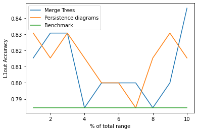
A concise summary of the results can be found in Figure 4, while Table 1 in the supplementary material reports more detailed prediction errors obtained after L1out cross-validation. As in Sangalli et al. (2009b), we obtain the best classifier by simultaneously considering the combined information conveyed by the couple of curvature and radius functions; the dissimilarity between different couples is measured by the distance in Equation 1, where the parameter being this the value which minimizes prediction error computed by L1out.
The same pipeline is followed when curvature and radius functions are represented by merge trees or by persistence diagrams. In the case of PDs’, we first removed the points (that is, the topological features) with persistence lower than a certain threshold (where the persistence is , according to the notation used in Section 3). The threshold has been taken equal to the pruning parameter of the merge trees, in accordance with 6.
From the results we obtained (see the first two rows in Table 1 in the supplementary), we observe that PDs do a slightly better job in extracting useful information from either curvature or radius, when examined separately. This could be due to a situation not dissimilar from that illustrated in the example of Section B.1 in the supplementary material: the discriminant information contained in the curvature and radius functions lies more in the number and amplitude of oscillations than in their ordering. However, when curvature and radius of the ICA are jointly considered as descriptors and the distance of Equation 1 is used, we obtain a better classifier for merge trees while there is no improvement for PDs.
This situation highlights that merge trees and persistence diagrams capture different but highly correlated pieces of information about the current functional data set; note, however, that PDs suggest that most of the information they capture is due to the radius function, while merge trees show some informative interactions between curvature and radius.
The number of patients misclassified by the best classifier based on merge trees is slightly smaller than that of the best classifier based on PDs - see Figure 4, but, despite the profound differences between the two topological summaries (see Section 4, Section B.1, Section B.2 and Section B.3) the two methods are retrieving similar discriminant information related to the classification task: comparing the two analysis we found that patients were misclassified by both methods. For comparison, the prediction errors of the best classifiers based on merge trees and on PDs are reported in the third column of Table 1 in the supplementary material, while in the last row the reader can find the prediction errors of the classifier described in Sangalli et al. (2009b).
7.2.4 Robustness with respect to the pruning threshold
To argument in favor of the robustness of our results with respect to the choice of the pruning threshold, or, from another point of view, in favor of the robustness of the information conveyed by our tree representation of functions, we go through the same classification pipeline varying the value of the pruning threshold of the radius functions. In Figure 4 we show the prediction accuracy, estimated by L1out cross-validation, as a function of the pruning threshold. We notice that the accuracy is quite stable and does not oscillate wildly upon perturbing the pruning threshold. This fact, on one hand further supports the elbow analysis approach described in Section 7.2.2, on the other is also showing that the results obtained with the information captured by merge trees and persistence diagrams does not depend on a finely tuned choice of the threshold parameter.
8 Discussion
We believe that methods from TDA can be fruitfully added to the toolbox of functional data analysis, especially when non trivial smoothing and alignment are required for data representation. In this paper we focused on two topological representations of functions: persistence diagrams, which, being the most classical tool in TDA, are regarded as a benchmark, and merge trees, which are rarely used in real data analysis applications. The framework for merge trees is the very recent metric structure defined in Pegoraro (2021b), for which we also developed theoretical results specific for the application to functional data.
To support our narrative, we used as paradigmatic real world application the classification analysis of the AneuRisk65 functional data set. This data set poses all the desired challenges: careful smoothing procedures and alignment techniques must be employed to obtain meaningful results. Reanalyzing the seminal case study described in Sangalli et al. (2009b), we showed the advantages of having a representation of functional data which is invariant with respect to homeomorphic transformations of the abscissa – thus lightening the burden of careful alignment – and also allows for agile smoothing – possibly causing some overfitting – thanks to the pruning of the trees which takes care of this aspect of FDA which practitioners often find problematic. Following a classification approach based on QDA applied to properly reduced representations of the data, as in Sangalli et al. (2009b), we obtain robust results with comparable, if not better, accuracy in terms of L1out prediction error, and we confirm some facts about the variability of the data in the groups of patients characterized by the different location of the cerebral aneurysm, consistently with the findings of previous works.
The effectiveness of the simple pipeline proposed in the case study does motivate further research in order to deal with more complicated scenarios including multivariate functional data in which a vector of functions defined on the same domain could be summarized via a topological representation. Similarly, statistical tools to better interpret population of trees should be studied and developed, starting for instance from the brief discussion carried out in Section E. This would open up the door for more refined statistical procedures like testing or uncertainty quantification, which are very hard to deal with in general metric spaces. On top of that, optimizing the numeric and computational aspects of the tree-based tools that we introduced would surely make them more viable in applications.
To be sure, we want to stress that careful smoothing is still mandatory when precise differential information about the data is needed, since small oscillations in a function can still cause high amplitude oscillations in the derivatives, which cannot be removed by pruning. Moreover, not all FDA applications are adapted to the representations offered by merge trees or persistent diagrams. Indeed, the information collected by merge trees is contained in the ordering and in the amplitude of the extremal points of a function, and not on their exact abscissa. Hence, if the abscissa carries valuable information for the analysis – for instance, a wavelength, or a precise landmark point in space or time – the TDA approach followed in this work for data representation is not indicated, precisely because of its invariance property with respect to homeomorphic transformations of the abscissa. But this criticism also applies to many alignment procedures proposed in the literature. Similarly, in the supplementary material, Section B.2, we point out that there are functions which have equivalent representations in terms of merge trees although the order on the abscissa of their critical points is different, in spite of the fact that merge trees are much less sensitive to such issue when compared to persistence diagrams (see also Kanari et al. (2020)). If the order of critical points of the function is of importance for the analysis, then surely persistence diagrams, but possibly also merge trees, should be avoided.
More generally, we point out that whenever the datum designating a statistical unit is only a representative of an equivalence class, the analyst must be sure that the variability differentiating the members of the same class is ancillary with respect to the statistical analysis performed on the statistical units. This consideration always applies in FDA, whenever data are aligned according to transformations belonging to a group. Merge trees offer a representation of functional data in terms of equivalence classes whose members are invariant with respect to homeomorphic transformations of the abscissa. Persistence diagrams partition the space of functional data in even coarser equivalence classes, although they could be enough for the analysis, as we saw in the case study illustrated in Section 7. Occam’s razor should guide the analyst’s final choice.
A Topological Remark
In Section 2.3 we make some selective assumptions on and , to make sure that along the filtration topological changes only happen at critical values, that is: for a critical value , for all small enough, is bijective. In 1 we point out that this fact boils down to the topology of the sets:
for every critical point and for every . Topological changes happening at the critical values are equivalent to always being non empty and path connected. This in general does not hold as we can see in the upcoming examples.
Example I
Consider the following sequences of topological spaces and . For let and . Moreover, let . and share the same set of critical values, namely and they only differ by the number of path connected components at the critical value : , while . In changes happen across the critical values - and , while in changes happen at the critical values - and .
Example II
Consider the following sequence of topological spaces . For let and Then however has two path connected components while, for the set is path connected.
Example III
Let defined by Let be the closure in the plane of the set , which is given by . The set is usually referred to as the topologist’s sine curve and the set as the closed topologist’s sine curve. Let be:
That is, is an -thickening along the -axis (second component of ), of the graph of restricted on the interval . Thus, if we add to the rectangle we obtain a set such that:
-
•
-
•
is compact and path connected. It is in fact homeomorphic to and thus homeomorphic to a closed disk in the plane.
As we obtain a family of compact ”disks” whose intersection is which is not path connected.
Example IV
Lastly with being . Clearly is closed and path connected, but is empty.
In all the examples above we see different situations in which at some critical point we have a very “unstable” topological scenario, which changes at for any small :
-
•
in Example I the balls centered in and contained in touch right after ; in fact their closures (giving ) at would intersect;
-
•
in Example II the horizontal stripe given by suddenly disconnects at because it is no more thick enough to get around the hole in ;
-
•
we find a very similar situation also in Example III, where every thickening of would allow us to bridge between its two path connected components;
-
•
lastly, in Example IV, we have a path connected component being born with a minimum “lying” at , thus producing an empty level set at .
The general point of view which we assume, which is formalized in Pegoraro (2021b), is that we deem to be negligible the topological differences between and in Example I, as those two filtrations have the same path connected components but for one point, , which we may look at as a measure zero subset of the parameter space indexing the filtration (i.e. ). Thus, for all these examples, and, in fact, for all the tame filtrations of path connected topological spaces, we propose to build the associated merge tree as if all topological changes happen at critical points: if we have a critical point such that is not bijective, instead of looking at the merging information contained in - as we do in Section 2.3 - one should look at , but still recording the topological changes with a vertex at height . In this way, for instance, the merge trees associated to and in Example I would be the same, in Example II we would have a single leaf at height - despite having two path connected components, the same for Example III (upon replacing with ), and, lastly, Example IV would feature a leaf at height despite being empty.
B Examples
In this section, we present some examples which are intended to put to work the pruning operator and further show the differences between persistence diagrams and merge trees, already highlighted in Section 4 of the manuscript.
We devote Section B.1 to giving further intuition on the topic of functions being distinguished by merge trees but being represented by the same persistence diagram. Section B.2 and Section B.3 instead give a more qualitative idea of what kind of variability between functions is better captured by PDs and merge trees with, respectively, the -Wasserstein metric and the edit distance. Lastly Section B.4 deals with the problem of pruning trees to remove ancillary features.
B.1 Example I
In this first example we produce a set of functions which are all described by the same persistence diagram but are distinguished by merge trees.
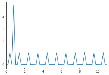
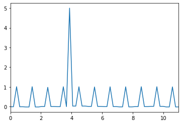
We want to exploit that, for continuous functions in one real variable, the merging structure of the path connected components (and so the tree structure ) is characterized by how local minima distribute on different sides of local maxima. We create a very simple toy situation: we define functions which have all a very high peak and a number of smaller peaks of the same height, but with a different disposition of these smaller peaks with respect to the highest one.
For , let be such that on while, on , is the linear interpolation of , and . Then, for , define as on while, on is the linear interpolation of , and .
Then, for , is obtained as follows:
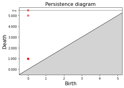
The functions and are displayed in Figure 5(a). Note that the first and the last peak of every function, by construction, are always small peaks. The key point is that for every path connected component we are not changing any of the corresponding critical values and thus the associated persistence diagram is always the same (see Figure 5(c)).
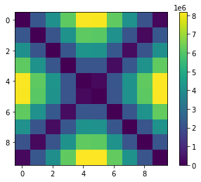
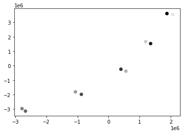
The shortest edit path between two merge trees and is given be the deletion of one leaf in each tree to make the disposition of leaves coincide between the to trees. The more the peak disposition is different between the two trees, the more one needs to delete leaves in both trees to find a shortest path between them. Thus, if we fix the first line of the matrix in Figure 5(d), we see that going left-to-right the distance at first gradually increases. It is also evident that, from a certain point on, the distance decreases to the point of reaching almost zero. This is because the first function (the one in which the highest peak is the second peak) and the last function (the one in which the highest peak is the second-to-last peak) can be obtained one from the other via a -axis symmetry and a translation – (reflection on the -axis) and , with fixed (translation) –, these transformations being homeomorphisms of the abscissa. Similarly, the second function is equal, up to homeomorphic alignment, to the third-to-last one, etc.. Thus by 1 the merge trees are the same. To sum up the situation depicted in the first row of Figure 5(d), first we get (left-to-right) farther away from the first merge tree, and then we return closer to it. This intuition is confirmed by looking at the MDS embedding in of the pairwise distance matrix (see Figure 5(e) - note that the shades of gray reflect, from white to black, the ordering of the merge trees). The discrepancies between the couple of points which should be identified are caused by numerical errors.
B.2 Example II
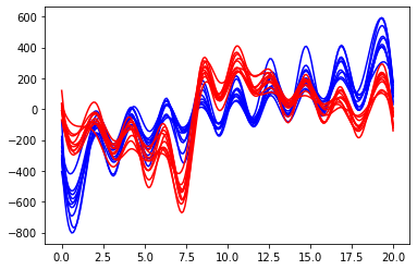
In this second example we want to produce a situation in which the variability between functional data is better captured by PDs than by merge trees. Accordingly, we generate two clusters of functional data such that membership of a function to one cluster or the other should depend on the amplitude of its oscillations and not on the merging structure of its path connected components. We then look at the matrices of pairwise distances between functions, comparing merge tree and persistence diagram representations in terms of their goodness in identifying the clustering structure.
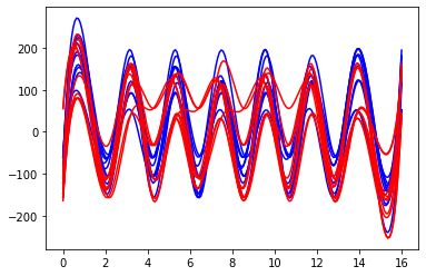
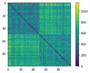
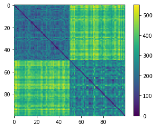
To generate each cluster of functions, we draw, for each cluster, an independent sample of 16 critical points, 8 maxima and 8 minima, from two univariate Gaussian distributions with means equal to for maxima and to for minima, respectively. The standard deviations of the two Gaussian distributions are the same and they are set equal to To generate a function inside a cluster, we draw a random permutation of 8 elements and we reorder, according to this permutation, both the set of maxima and the set of minima associated to the cluster. Then, we take a regular grid of 16 nodes on the abscissa axis: on the ordinate axis we associate to the first point on the grid the first minimum, to the second the first maximum, to the third the second minimum and so on. To obtain a function we interpolate such points with a cubic spline. We thus generate functions in each cluster. The key point is that, within the same cluster, the critical points are the same but for their order, while the two clusters correspond to two different sets of critical points.
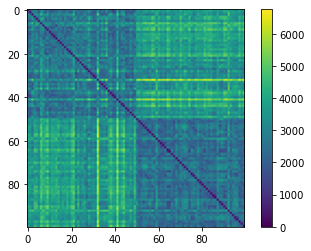
In this example, we expect that the clustering structure carried by the amplitude of the functions will be shadowed by the differences in the merging order, when adopting the merge tree representation; while persistence diagrams should perform much better because they are less sensitive to peak reordering. This is in fact confirmed by inspecting the distance matrices in Figure 6(b) and Figure 6(c).
B.3 Example III
Here we reverse the state of affairs and we set the feature for discriminating between clusters to be the merging structure of the functions. Hence, we generate two clusters of functions: the members of each cluster have the same merging structure which is however different between clusters.
To generate the two clusters of 50 functions each, we first draw an independent sample of 10 critical values, maxima and minima, shared between the clusters. Such samples are drawn from Gaussian distributions with means and respectively and standard deviation . Given a regular grid of nodes on the abscissa axis, on the ordinate axis we associate to the first point of the grid a maximum, to the second a minimum, and so on, as is Example I. To generate every member of one cluster or the other, we add to the ordinate of each maximum or minimum critical point a random noise generated by a Gaussian with mean 0 and standard deviation . Then we reorder such points following a cluster-specific order. And, lastly, we interpolate with a cubic spline. We remark that the ordering of the maxima and that of the minima now becomes essential. For the two clusters, these orderings are fixed but different and they are set as follows ( indicates the smallest value and being the largest value):
-
•
first cluster: maxima are ordered along the sequence , minima along the sequence ;
-
•
second cluster: maxima are ordered along the sequence, minima along the sequence .
Such different orderings provide non-isomorphic tree structures for the merge trees associated to the functions of the two clusters, as we can see in Figure 7(a), while keeping a similar structure in terms of persistence diagrams.

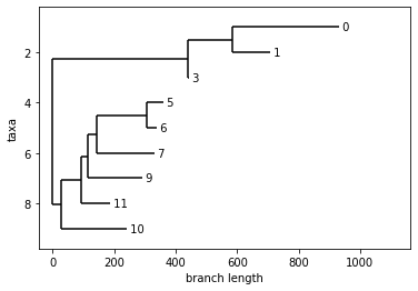
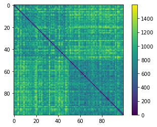
In this example, we expect to be unable to recognise the clustering structure among the data; indeed, the only discriminant feature available to is the different height of critical points, but this bears little information about the clusters.
We can visually observe this by comparing Figure 7(c) with Figure 7(d).
B.4 Pruning
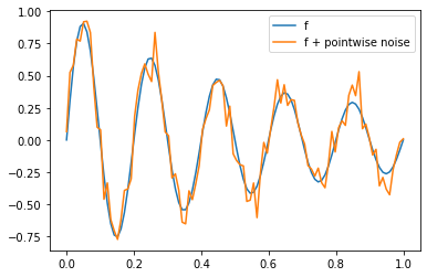
In this section we present a simple example to show the regularization effect of pruning, along with an elbow analysis to identify a suitable pruning threshold. Figures related to this example can be found in Figure 8.
Consider the function defined for , and fix a grid on . Consider a function which, on the fixed grid, could be considered as a noisy observation of : with i.i.d.. We want to study the relationship between the merge trees built from the samples and (via linear interpolation). With an abuse of notation we call such merge trees, respectively, and .
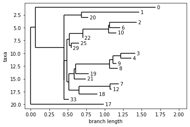
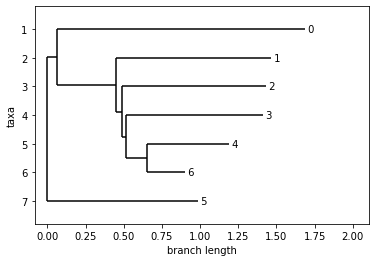
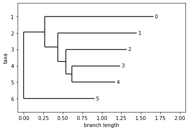
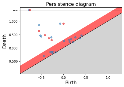
Knowing the generative model, in each point of the grid, with probability we expect to see a value of at a distance at most from the corresponding value of Thus, a pruning threshold of around should be enough to cope with most of the noise in . But this information can be retrieved directly from data with an elbow analysis: for every we consider the number of leaves in and we plot the curve obtained by varying . Under the assumption that the signal to noise ratio is high, we should identify an elbow in the curve vs number of leaves of . In fact, this corresponds to having some separation between noisy oscillations and the proper shape of the function. If that is not the case, it means that there are oscillations caused by noise which are at least as big as some oscillations which we would like to retain. Thus the smoothing parameter choice in this case is more arbitrary and some kind of compromise must be achieved. Note that there might be multiple elbows in the aforementioned plot, along with flat regions. A conservative choice would be to look for the leftmost clear elbow, which, for instance, may be recognized at in Figure 8(c). We can appreciate that the flat region (meaning that does not change) starting in contains also . Lastly, we highlight that, despite the pruning procedure, the amplitude of the larger oscillations, which are retained in the pruned tree, is still affected by the noise.
An analogous result can be achieved also working with persistence diagrams, where, instead of an elbow analysis, one has to choose a band close to the diagonal, as shown in Figure 8(f), which contains all the small persistence features which one wants to eliminate. The band in Figure 8(f) has width . As for merge trees, if there is not clear separation between close-to-diagonal noisy points and more persistent features, one needs to make some arbitrary choice to fix a suitable band. For -filtration of point clouds in there are bootstrap methods to obtain confidence bands (Fasy et al., 2014).

C Spline Spaces
We use this section to emphasize for spline spaces the consequences of the results of Section 6, since splines are often used in FDA applications for smoothing the discrete raw data profiling each statistical unit in the sample.
As already noted in the introduction of the manuscript, spline spaces are a preferred tool for smoothing functional data since they provide finite dimensional vector spaces of functions with convenient properties. In particular, spline functions are piecewise polynomials determined by a grid of knots; fixing the knots determines a finite upper bound for the number of critical points of the spline. Consider for instance , the space of piecewise cubic polynomials over a grid on with equispaced knots. On each interval the first derivative of the function is a quadratic polynomial and thus its zero set is composed by at most two points. This means that the number of critical points of is at most ; therefore the number of leaves of the tree associated to cannot be greater than . The following Corollary of 1 is in fact easily obtained:
Corollary 2
Let be a space of piecewise polynomial functions of some fixed degree, all defined by means of the same finite grid of nodes. Then the operator is continuous.
Smoothing raw data with splines entails a delicate trade-off between being flexible, to capture the salient features of the function the raw data have been sampled from, and avoiding the introduction of artifacts, due, for instance, to noise overfitting or caused by forcing the spline to fit an abrupt spike. Representing the smoothed spline function by means of a merge tree can help in handling this trade-off, by allowing the analyst a certain degree of casualness in the smoothing phase, since the small artifacts generated by a possible overfitting will then be controlled by pruning the tree.
For instance, consider the problem of approximating with a cubic spline function defined by an equispaced grid of knots. Suppose satisfies some regularity conditions, usually implied by its embedding in a Sobolev space. The parameter which controls the bias-variance trade-off is just the number of knots . Many results are known in the literature concerning the uniform convergence of spline functions as the step of the grid of knots goes to zero (see for instance De Boor and Daniel (1974)) and most of them are given in terms of a factor and the norm of the derivatives or the modulus of continuity of . In other words, the pointwise error can be reduced as needed by increasing . When is approximated by the spline function with an error of in terms of uniform norm, this means that whatever happens in intervals of around is inessential. Stated in different terms, oscillations of taking place in such zone are to be considered uninformative with respect to the analysis. Thus a sensible choice is to represent the function fitted by the spline by means of the pruned merge tree . If is small enough with respect to the oscillations of , 1 implies that pruning by removes only inessential edges of , without losing important information about .
The same argument applies when smoothing observations sampled from a function The analyst may allow the spline to slightly overfit the data and then decide that oscillations under a certain amplitude are irrelevant, controlling them by pruning the merge tree associated to the fitted spline.
D Clustering
In this section, we present an unsupervised exercise with the aim of clustering patients on the basis of the similarity of geometric features of their ICA. We explore the Aneurisk65 data clustering structure by endowing the merge tree space with the metric figuring in Equation 1 (contained in the paper), with . To get multiple perspectives on this issue, we resort to hierarchical clustering dendrograms with different linkages. The visual inspection of Figure 17 of the manuscript suggests that, upon blending together the information of radius and curvature, the Upper class should display a low variability while the Lower and None classes should behave more heterogeneously. Thus, a clear clustering structure should not be recognizable: we expect possibly one cluster made by points belonging to the Upper class and then a series of points scattered around this central nucleus with no easily recognizable pattern.
The hierarchical dendrograms obtained with single, average and complete linkages are displayed in Figure 9. The first obvious observation is that all three linkages identify the point associated to patient as an outlier. The single linkage dendrogram shows that, as the height on the dendrogram increases, there is only one major cluster which slowly becomes larger and incorporates all points in the data set. No other relevant clusters are found. Average and complete linkages further support this finding: there are no obvious heights where to cut the tree in the average linkage dendrogram; complete linkage instead shows perhaps a two cluster (plus one outlier) structure. The smaller cluster identified by this dendrogram, is also visible with the average linkage and is contained within the group of singletons obtained by cutting the single linkage tree at height . The overall picture is thus that of a major cluster, with possibly another group of points clustered together, but with much higher heterogeneity.
These findings can indeed be related with the labels declaring membership of the patients to the the and the group respectively. To grasp if there is an overall pattern in the merging structure of the data point cloud, for each leaf (a patient) of a dendrogram, we collect its merging height defined as the height of its father in the graph, that is the height at which that point is no longer considered as a singleton but instead it is clustered with some other point. In other words, we record the distance between the leaf and the closest cluster in terms of the cophenetic distance induced by the dendrogram. Note that, for the single linkage dendrogram, this is equivalent, for almost all leaves, to the height at which the leaf is merged with the major cluster. Results are shown in Figure 10. The interpretation of these plots is consistent across the different linkages and is pretty straightforward: the points corresponding to patients of the Upper group get merged within a small range of heights, and the distribution of their merging height is stochastically smaller than the distributions for groups and respectively. The merging heights of the leaves corresponding to patients belonging to the Lower group, instead, display a larger variability and their distribution is stochastically larger than those of the of the leaves belonging to the other two groups. Patients of the class None, merge at heights in between the Upper and the Lower groups and their merging height seems to display a low variability. The plot (d) of Figure 10 shows the smoothed densities of the distributions of merging height for leaves belonging to the three groups, in the case of average linkage. Analogous representations could be obtained for the other two linkages; they all confirm the stochastic ordering described above.
This cluster analysis is consistent with our expectations, which, in turn, are in accordance to the findings of Sangalli et al. (2009b). On top of that, we also get two further insights: first, data are scattered around the Upper group with a possibly non uniform structure, as shown by the small and sparse cluster of Lower class patients visible with complete linkage clustering and, second, that the None group of patients lies in a sort of in between situation in the space separating the two other groups of aneurysm-affected patients. This could also explain the good performance of QDA: a quadratic boundary is able to isolate the core of the Upper group of patients from the others, which lie mainly on one side of the quadratic discriminant function.
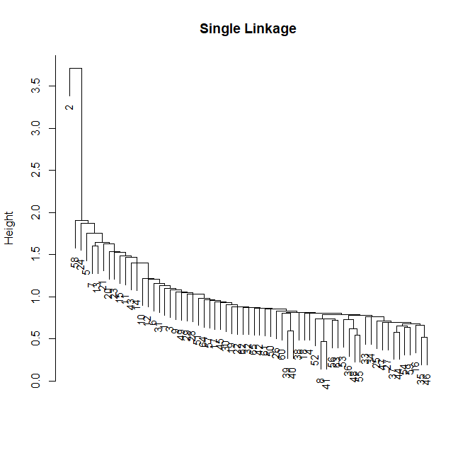
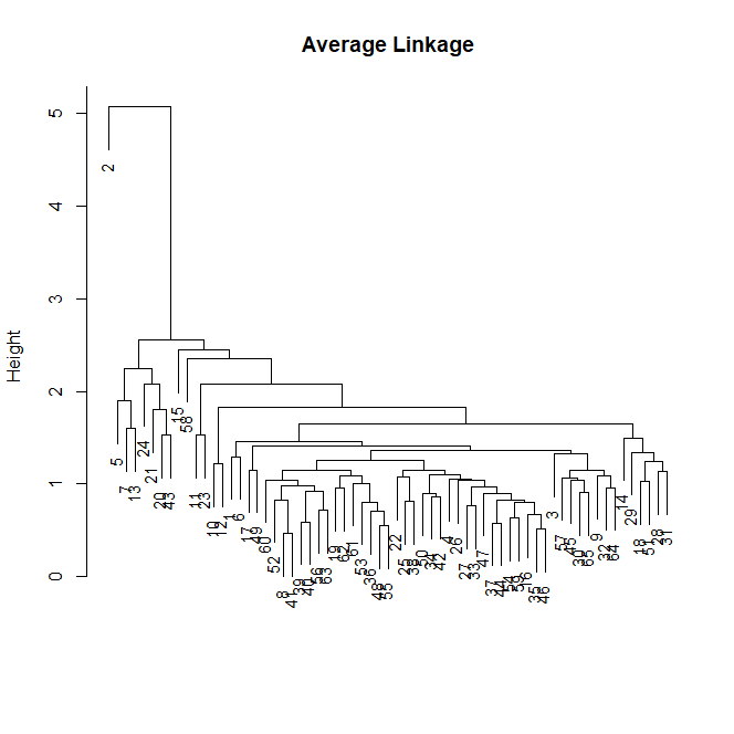
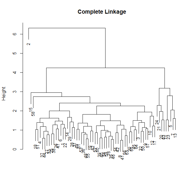
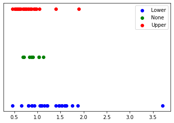
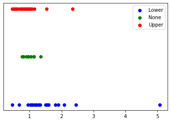
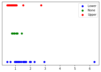

E Reading the trees
Though not strictly related to the classification task presented in Section 7 and the clustering carried out in Section D, we take the opportunity to briefly investigate the population of trees obtained from the Aneurisk data set to see what can be said about the different groups (U,N,L) and to try to explain the effectiveness of the proposed analysis. This is intended as a first step into developing further statistical tools to interpret and understand populations of merge trees.
A path which has been taken to produce summary statistics of a topological representation - in particular a persistence diagram - is to obtain a function for each topological summary and then use consolidated (functional) statistical methods to analyze the obtained curves (see for instance Sørensen et al. (2020)). We will do the same, producing a curve for every merge tree, in three different ways.
It must be immediately pointed out that the relationship between the topological representation and the chosen summary functional statistic should be formally addressed in a number of ways. For instance, pointwise or uniform convergence of the functional summaries when diagrams/merge trees/etc. are close according to some metric should be studied as well as the injectivity of the functional representation of the topological summary. These aspects of topological data analysis up to now have been hardly explored in the literature; they require efforts and space which are outside the scope of the present work. Our aim here is just to showcase qualitatively the discriminative power, in our case study and examples, of some functional statistics in order to foster and motivate further efforts on the topic.
We make use of the following definition.
Definition 7
Let be a merge tree; cutting at height generates the set of merge trees .
Now, consider a merge tree associated to a function , with compact interval in Cutting at height , means looking locally at the oscillation patterns obtained by removing from the domain of the super level set : the different subtrees represent the function restricted to the different path connected components of . Thus each subtree describes locally the function , with controlling the resolution of these descriptors. Based on this fact, we introduce the following functional statistics. For each tree and for each we look at:
-
1.
: the variance of . With this statistic we capture how the already completed oscillations of are grouped together, focusing on the homogeneity of these patterns: high variance suggest that the merge tree is very unbalanced below height , implying that oscillations completed below are more concentrated in some regions of the domain compared to others. Low variance, instead, indicates that oscillations are more evenly distributed;
-
2.
: the statistic counts the oscillations which have already started at height ;
-
3.
: the statistic counts the oscillations which have been completed before height .
Note that the first statistic we present is strictly related to information contained in merge trees and so it does not apply to persistence diagrams; the last two, instead, respectively count the number of components born before and the ones which have died before time . These statistics can also be computed for persistence diagrams.
Letting vary in for every tree we obtain a curve, a functional statistic. These curves can then be aggregated over different subsets partitioning the population of trees.
E.1 Examples in Section B
To gain confidence with these tools, we look at the simulated scenarios presented in Section B.1, Section B.2 and Section B.3 through the lenses of these statistical summaries. The reader can follow the next paragraph looking at Figure 11.
The first example, Section B.1, presents a data set of functions such that the associated merge trees are distinguished just by the tree structures: in fact the associated persistence diagrams are all equal. Each tree as a total of leaves, the father of each leaf is at height and cutting each tree between heights and yields two clusters. Thus, the only difference between the trees lies in the cardinality of such clusters. Accordingly, the only statistic which is able to separate them is the variance between the clusters cardinalities: we clearly see that in Figure 11(a). The other plots, as expected, show perfectly superimposed curves.
The second example, Section B.2, presents data divided into two groups with the discriminant information between the groups lying into the heights of the critical points of the functions. Figure 6(b) and Figure 6(c) show that both merge trees and persistence diagrams can distinguish, to some extent, the two groups, with persistence diagrams being able to identify them more clearly. Figure 11(e) and Figure 11(h) show that the groups have two very distinct behaviors in terms of births and deaths of path connected components: as the height parameter runs through the heights of the merge trees, we can clearly see that shaded areas of the different classes are well separated. Moreover, in Figure 11(b) we see that we have a lot of within-group variability generated by tree structures, which is in perfect accordance to the generative process of the data set. This further explains why persistence diagram do such a good job in separating the two groups.
The third example reverses the situation: births and deaths of path connected components should not present different patterns in the two groups, while the tree structures involved should present profound differences between groups. From Figure 11(f) and Figure 11(i) it is quite evident that heights of local minima and maxima do not contain enough information to separate groups. Instead Figure 11(c) shows that while Group 1 presents very balanced tree structures, for is very low for high, Group 0 has very imbalanced merging structures, with many components being merged together and few standalone ones appearing/merging late.
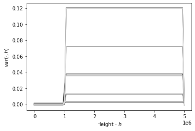
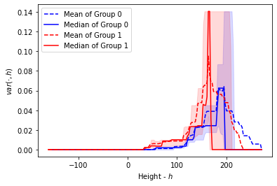
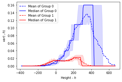
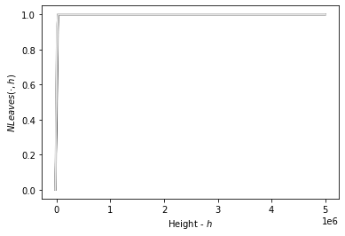
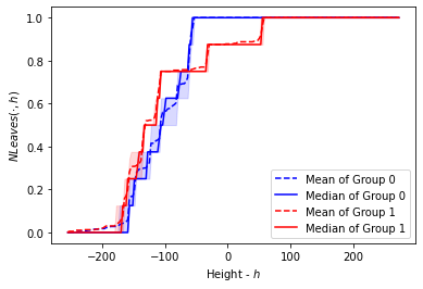
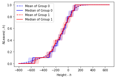
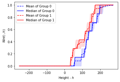
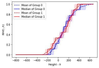
E.2 Aneurisk65 Case Study
In this section we illustrate for the Aneurisk65 case study the same analysis obtained in Section E.1 for the simulations described in Section B.1, Section B.2 and Section B.3.
E.2.1 Curvature
First we focus on the analysis of the merge trees obtained from the functions recording the curvature of the blood vessels centrelines. In the first row of Figure 12 we see the plots of the statistics we want to discuss.
Figure 12(a) tells us that the tree structures of the three classes exhibit quite different behaviors: we see that L tend to be more imbalanced than N and U (especially looking at the median values), but both L and N have many outliers which cause median and mean values to be very different. However, due to the within-group variance it is not possible to discriminate between groups using such statistic, as the shaded area of group L includes the areas of the other classes. Still, we can appreciate that class U shows much less within-group variance compared to N and L. Figure 12(b) and Figure 12(c), together, carry the following information: class U tends to have less oscillations compared to class L. Moreover, such oscillation tend to take place at lower values, as the red curves flatten before the blue one. Class N instead lies in between the other two groups.
To conclude, the differences we can spot in the merge trees associated to curvature functions lie mostly in the number of oscillations and in their height, with class U being generally more characterized (i.e. with smaller within group variance) then the other classes. Not much remnant discriminating information seems to be contained into the tree structures of the different groups.
E.2.2 Radius
Now we turn to merge trees associated to radius functions - second row of Figure 12.
Figure 12(d) depicts a situation which is not very different from Figure 12(a), even if the roles of the different labels are exchanged: we have group U showing very high variability for high values of , with ouliers being present for all groups - the pointwise means end up outside the shaded regions. Both Figure 12(d) and Figure 12(a) may indicate something related to radius/curvature happening at the extremes of the domain, in particular for class U (radius) and L (curvature). However, as for curvature, these patterns do not discriminate between the groups L, N, U due to the within group variance being very high. Figure 12(e) and Figure 12(f) tell us that the class U, again, has consistently less oscillations than L and N. On top of that, class L tend to have lower minima and higher maxima than class U.
To sum up, the radius functions of class U have less oscillations, compared to L and N, and the overall amplitude of such oscillations is also smaller.
E.2.3 Conclusion
Putting together the information collected in the previous subsections we can say that the curvature functions associated to patients in group U oscillate less then the other groups, with their peaks being lower than the ones of L and N. The radius functions of the group U still oscillate less in terms of numbers of local minima and amplitude of the oscillations.
In other words, blood vessels from group L are more wiggly in the space (and thus their curvature oscillates more, touching higher values) and their diameter oscillates more frequently and by a greater amount compared to class U. These features might indeed be associated to different blood fluid dynamics regimes characterizing patients in group U. Group N lies in between, some patients showing patterns closer to group L and some others to group U. Being the groups L,N,U characterized by this topological information, we can see why both merge trees and persistence diagrams perform well in the pipelines presented in the manuscript. At the same time, the fact that the tree structures do not show particular patterns - Figure 12(a) and Figure 12(d) - could explain why merge trees and persistence diagrams perform similarly.
The work of Sangalli et al. (2009b) reports that the geometrical features found relevant to describe the data - namely: the overall width of the ICA, its tapering effect, the curvature of the ICA in proximity of the last peak of curvature and the curvature along the segment of the ICA between the two peaks of curvature - show a lower variance for the group U, when compared to group L; and patients in group U tend to have a wider and more tapered ICA’s than those in group L. They also present a less curved ICA between the two peaks of curvature. We can appreciate that our findings are in accordance with the ones of Sangalli et al. (2009b): indeed, we found in Section D that the group U exhibits a much smaller variability in terms of merge trees, being its trees clustered together much more than the trees of the other groups. Similarly the information we capture on curvature and radius are coherent. Nevertheless we can also appreciate how the two approaches complement each other: Sangalli et al. (2009b) are able to identify differences in precise locations of the ICA, while the differences in terms of global oscillating behaviors and regimes are much better captured by the topological summaries.
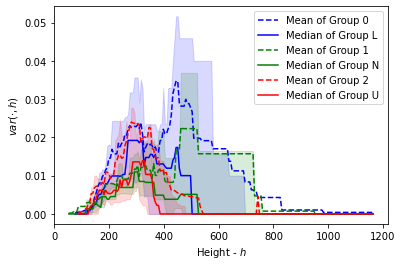
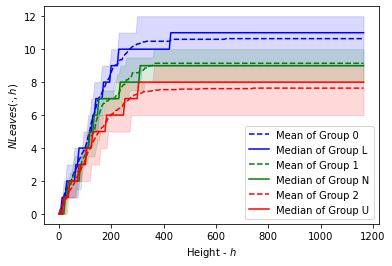
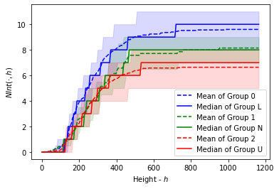
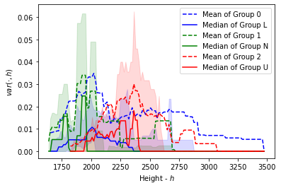
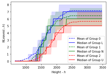
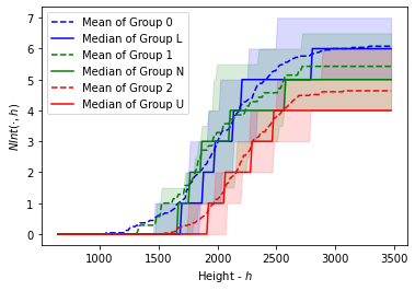
F Additional figures and Tables


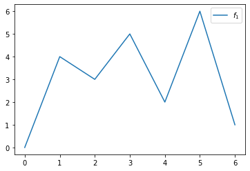
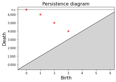
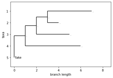
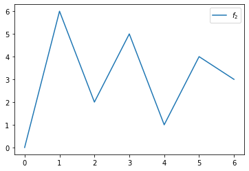

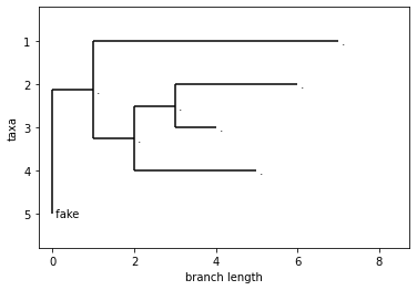
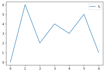

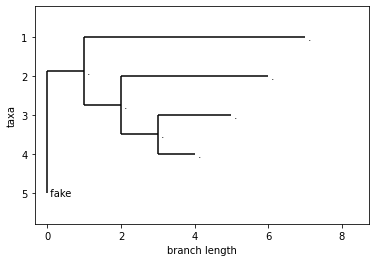
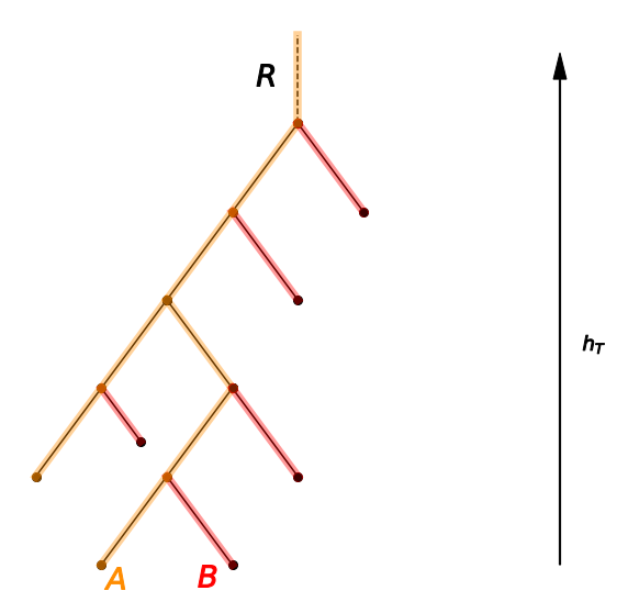
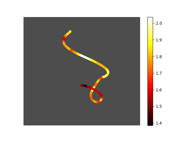
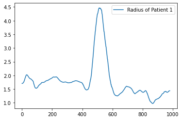
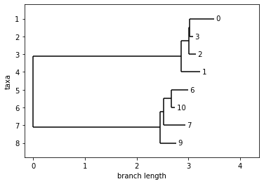
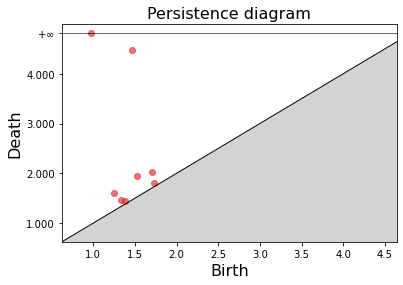
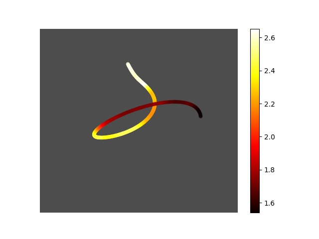
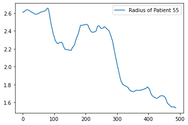
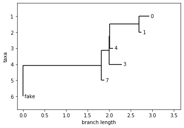
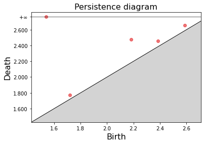
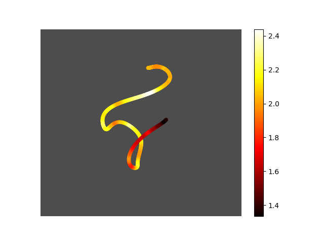
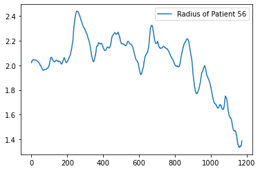
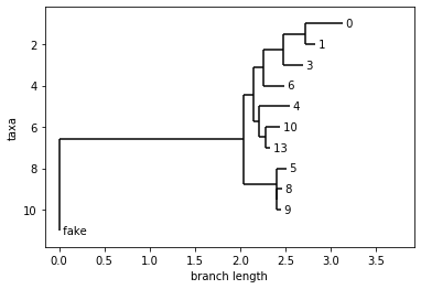

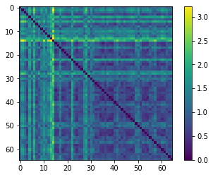
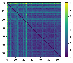
| Merge Trees | |||||||||||
| Predicted | |||||||||||
| Curvature | Radius | Mixed | |||||||||
| True | U | LN | U | LN | U | LN | |||||
| U | 18 | 14 | U | 24 | 8 | U | 26 | 6 | |||
| LN | 3 | 30 | LN | 7 | 26 | LN | 5 | 28 | |||
| , | , | , | |||||||||
| Persistence Diagrams | |||||||||||
| Predicted | |||||||||||
| Curvature | Radius | Mixed | |||||||||
| True | U | LN | U | LN | U | LN | |||||
| U | 20 | 12 | U | 26 | 6 | U | 26 | 6 | |||
| LN | 3 | 30 | LN | 6 | 27 | L | 6 | 27 | |||
| , | , | , | |||||||||
| Benchmark | |||||||||||
| Predicted | |||||||||||
| U | LN | ||||||||||
| True | U | 26 | 6 | ||||||||
| LN | 6 | 27 | |||||||||
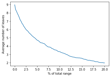
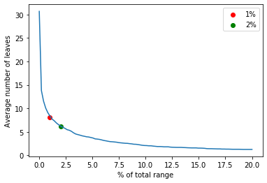
G Proofs
Proof of 1.
Let be a bounded function defined on a path connected topological space and let be an homeomorphism. We need to prove that the merge tree and the persistence diagram associated to the function and are isomorphic.
We know that:
This means that if and only if , and so . Since the restriction of an homeomorphism is still an homeomorphism, we can take its inverse, and by the composition properties of , we obtain that . Given , we thus have the following commutative diagram:
and passing to path connected components/homology:
where the vertical arrows in the second diagram are isomorphisms of groups. The first diagram then gives the isomorphism of merge trees, while the last one gives the isomorphism of and .
Proof of 2.
Each leaf in corresponds to a point in . The coordinate of each point is given by its height, which can be retrieved through . Consider and let be the ordered set i.e. the path from towards . The coordinate of the points associated to is the minimal height at which intersects another path , with being a leaf with height less than .
Proof of Lemma 1.
Let . Being continuous, is open in . Therefore and . For every open neighbor of we know and . By the continuity of , for every we have open neighbor such that for every , . In particular, we can always consider . Thus, for every we have and . Thus .
Proof of 3.
The leaf is associated to a path connected component , with and . Consider now and let . Being continuous is open in .
We can define such that if , and if .
We have ; in fact for every and if . Moreover if and for . And this implies the result about merge trees and tameness.
We only need to prove that is continuous. We need to verify that, for any , for every there is open neighbor of such that for every , we have . If this is trivially verified since is open and so we can always find , where is constant. If is an internal point of , still the condition is verified for and is continuous. We are left with the case . For every path connected open neighbor of , we know that . Moreover since is open in and it would imply that an internal point of . So and by Lemma 1, .
So if , then : if then otherwise . Thus, is continuous.
Proof of 1.
Starting from , each time we apply () to obtain from , thanks to 3 we have continuous tame functions and such that . Each is equal to up to an open set . Thus, if , then on . Note that either - with - or they are disjoint. The case occurs when at the -th step we delete a leaf such that - with being the leaf deleted at the -th step and with the father of being taken in , but being compared to in . If this is not the case, the sets and are disjoint.
We want to prove that .
We know that on we have and on we have . Thus .
Consider now , which is always non-empty. For we have . The key observation is that by construction a local minimum of over is given by any point in the path connected component associated to , i.e. there is such that and . Thus . The result on the merge trees follows by construction, since the deletions which lead to each are induced via pruning.
Proof of 1.
To prove the theorem, we need some notation and some auxiliary results. To avoid dealing with unpleasant technicalities we work under the hypothesis that for any merge tree , is an injective function. We call this assumption (G). It is not hard to see that for any fixed merge tree , for any , there is a merge tree such that (G) holds and . It is enough to make arbitrarily small shrinkings to the edges. Similarly for functions: given a continuous function we can always find an arbitrarily close function - in terms of - such that the associated merge tree satisfies (G).
First we define the least common ancestor (LCA) of a set of vertices in a merge tree.
Definition 8
Given a merge tree and set of vertices , we define .
Consider now tame functions on the path connected topological space such that . Let and be their associated merge trees. For we set . Since we have and of course .
We set , , , and . We then call and . With these pieces of notation we can write down the following commutative diagram:
Note that the diagonal maps are and . Lastly, if , we say that .
If we collect together the path connected components and taking the disjoint unions and we can write down the maps and , so that given , . Given , we also set . The same for .
We point out that the vertices of the merge trees and are contained in some or , respectively, and thus we have and . We will often refer to as , and thus, for instance, take , without explicitly mentioning the inclusion map. Note that the partial order we defined for and is compatible the the one of the vertices of the merge trees.
In a more technical language, and are the display posets of the two persistence sets and (Curry et al., 2022), but we want to avoid introducing such technical definitions. The work of Beketayev et al. (2014) shows that and give an -interleaving of merge trees (see Beketayev et al. (2014)), which, by Agarwal et al. (2018), is equivalent to the map satisfying the following conditions:
-
(P1)
for all
-
(P2)
if then there is such that , and .
-
(P3)
if , then, given , we have .
A map which satisfies (P1)-(P3) is called -good (Agarwal et al., 2018).
To bridge between the continuous nature of and and the discrete and , we define the following maps:
and similarly for . Leveraging on these definitions we set and .
Finally we start building an edit path between and . To do so we progressively add couples to an empty set : couples of the form mean that the vertex is deleted, while means that is deleted, means that the vertex is ghosted, means that is ghosted and means that we shrink so that the weight of becomes equal to the one of. The set is in very close analogy with the mappings defined in Pegoraro (2021b).
By working simultaneously on and , we collect all the “edits” in and then, in the last subsection of the proof, we use on induce an edit path between and . We will call the projection on the first factor, and the projection on the second.
G.1 Leaves of
In this section we take care of the leaves of the merge tree .
G.1.1 Selecting the Coupled Leaves
Consider the following set of leaves:
| (2) |
We name the condition:
so that we can more easily refer to it during the proof. Observe that we never have thanks to condition .
The set is the set of leaves which will coupled by : we add to all the couples of the form with and add for all .
Lemma 2
Given , then if and only if . Moreover, for every such that does not hold, there is such that .
Proof The first part of the proof reduces to observing that if and only if .
Now consider such that does not hold.
We know there is such that . If we are done, otherwise there is such that . Note that . Thus we can carry on this procedure until we find . Note that , thus, in a finite number of step we are done.
G.1.2 Height Bounds on Couples
Now we want to prove the following proposition which will be used to give an upper bound for the cost of the edits induced by the couples added to .
Lemma 3
Given , then .
Proof Suppose the thesis does not hold. Since , contradicting the thesis means that we have such that:
-
.
Let .
If holds, then .
Let . Note that . We have . But since , we also have
with which is absurd by Lemma 2.
G.1.3 Cost Bound on Deletions
In this step we prove a cost bound for some the vertices of which are going to be deleted. We add to the couples for every .
Lemma 4
Given , then .
Proof
We simply observe that, if then there
is such that . By property (P2) of , since , we have that has cost at most .
G.2 Leaves and deletions of
Similarly we add to the couples for every .
Lemma 5
Given such that , then .
Proof
Consider .
Let leaf.
We have and .
If we are done since .
Suppose instead .
This implies .
By construction , but then there is such that . Absurd.
G.3 Internal Vertices
Now we want to take into account the internal vertices of and .
Thanks to Lemma 4 and Lemma 5 we can delete all and such that , each with cost at most . Note that these deletions do not change the heights of any non deleted vertex.
Call and the two trees obtained after such deletions and after the ghosting of all the order vertices arising - and consequently adding or to for all the ghosted vertices respectively in or . If we consider then by construction . Similarly . Moreover . Thus is still -good. In what follows, with an abuse of notation, we avoid explicitly writing the restriction of the maps and , implying that these are always considered as defined on the “pruned” trees and .
G.3.1 Results on Internal vertices
We prove the following results.
Lemma 6
Let such that with . Let . Then .
Proof
For every we know and thus . Thus . Suppose then . However, for . Which is absurd for .
Lemma 7
Let such that with . Let with .
Then for every , let . Then we have .
Proof
Since but , we know . Suppose . We know for . But then which is absurd since .
Lemma 8
Consider , with . Let , with . Let . Then .
Since , then and similarly . Which entails and . Since , by Lemma 7 we have and, similarly, . Putting together , and and the analogous inequalities for we obtain .
Thus .
G.3.2 Deleting Internal Vertices
G.3.3 Coupling the Internal Vertices
After the deletions in Section G.3.2 we obtain two merge trees and , with the same leaves as and but with the property that for each we have a bijection between the leaves and the leaves in with . Thus for any edge we have a unique edge such that the leaves of and are in bijection and the same for and . Thus we can couple and , add to and make the shrinking to pair their weights. Since deleting a vertex doesn’t affect the weight of the other edges, then we can still apply Lemma 8 which guarantees that the shrinkings cost less then .
G.4 Inducing the Edit Path
To conclude the proof we sum up everything and induce and order edits operations according to the couples contained in , so that the costs of the edits matches the ones described along the previous subsections of the proof.
First we apply all the deletions on described in Section G.1.3, with the cost of every edit being at most . Then we ghost all order vertices. By construction we obtain, from , the tree . At this point we delete internal vertices of according to the procedure described in Section G.3.2, obtaining . Then we shrink all the edges of , according to Section G.3.3, obtaining . Then we insert all the edges needed to obtain from , which are associated to the couples mentioned in Section G.3.2. Then we go on with the splittings induced by , which are needed to subsequently insert the edges which take us from to , as explained in Section G.2. In the respective sections it is shown that all the edits we employed have cost less then .
This concludes the proof.
H Combining Metrics
To aggregate curvature and radius, we make use of the following proposition.
Proposition 4
Given and metric spaces, then , with and , is a metric on .
Proof
.
Since, given , is a metric if and only if is a metric, we can rescale and and take . We refer to as .
So:
-
•
iff and this happens if and only if .
-
•
symmetry is obvious
-
•
we use with and .
Since we get:
.
Therefore:
.
References
- Adams et al. (2017) H. Adams, Tegan Emerson, M. Kirby, R. Neville, C. Peterson, P. Shipman, Sofya Chepushtanova, E. Hanson, F. Motta, and Lori Ziegelmeier. Persistence images: A stable vector representation of persistent homology. Journal of Machine Learning Research, 18(1):1–35, 2017.
- Agarwal et al. (2018) Pankaj K. Agarwal, Kyle Fox, Abhinandan Nath, Anastasios Sidiropoulos, and Yusu Wang. Computing the gromov-hausdorff distance for metric trees. ACM Trans. Algorithms, 14(2), apr 2018.
- Beketayev et al. (2014) Kenes Beketayev, Damir Yeliussizov, Dmitriy Morozov, Gunther H. Weber, and Bernd Hamann. Measuring the distance between merge trees. In Topological Methods in Data Analysis and Visualization, pages 151–166. Springer International Publishing, Cham, 2014.
- Bhattacharya et al. (2015) Subhrajit Bhattacharya, Robert Ghrist, and Vijay Kumar. Persistent homology for path planning in uncertain environments. IEEE Transactions on Robotics, 31(3):1–13, 2015.
- Biasotti et al. (2008) Silvia Biasotti, Daniela Giorgi, Michela Spagnuolo, and Bianca Falcidieno. Reeb graphs for shape analysis and applications. Theoretical Computer Science, 392(1-3):5–22, 2008.
- Bille (2005) Philip Bille. A survey on tree edit distance and related problems. Theoretical Computer Science, 337(1-3):217 – 239, 2005.
- Bubenik (2015) Peter Bubenik. Statistical topological data analysis using persistence landscapes. Journal of Machine Learning Research, 16(3):77–102, 2015.
- Chazal et al. (2015) F. Chazal, Brittany Terese Fasy, F. Lecci, A. Rinaldo, and L. Wasserman. Stochastic convergence of persistence landscapes and silhouettes. Journal of Computational Geometry, 6(2):140–161, 2015.
- Chazal et al. (2016) Frédéric Chazal, Vin De Silva, Marc Glisse, and Steve Oudot. The structure and stability of persistence modules. Springer, 2016.
- Chung et al. (2009) Moo K. Chung, Peter Bubenik, and Peter T. Kim. Persistence diagrams of cortical surface data. In Information Processing in Medical Imaging, pages 386–397. Springer Berlin Heidelberg, 2009.
- Cohen-Steiner et al. (2007) D. Cohen-Steiner, H. Edelsbrunner, and J. Harer. Stability of persistence diagrams. Discrete & Computational Geometry, 37:103–120, 2007.
- Cohen-Steiner et al. (2010) David Cohen-Steiner, Herbert Edelsbrunner, John Harer, and Yuriy Mileyko. Lipschitz functions have lp-stable persistence. Foundations of Computational Mathematics, 10:127–139, 2010.
- Curry et al. (2021) Justin Curry, Jordan DeSha, Adélie Garin, Kathryn Hess, Lida Kanari, and Brendan Mallery. From trees to barcodes and back again ii: Combinatorial and probabilistic aspects of a topological inverse problem. arXiv, 2107.11212, 2021.
- Curry et al. (2022) Justin Curry, Haibin Hang, Washington Mio, Tom Needham, and Osman Berat Okutan. Decorated merge trees for persistent topology. Journal of Applied and Computational Topology, 2022.
- De Boor and Daniel (1974) Carl De Boor and James W Daniel. Splines with Nonnegative B-spline Coefficients. Mathematics of computation, 28(126):565–568, 1974.
- De Silva et al. (2016) Vin De Silva, Elizabeth Munch, and Amit Patel. Categorified reeb graphs. Discrete & Computational Geometry, 55(4):854–906, 2016.
- Dryden and Mardia (1998) I. L. Dryden and K. V. Mardia. Statistical Shape Analysis. Wiley, Chichester, 1998.
- Edelsbrunner et al. (2002) H. Edelsbrunner, D. Letscher, and A. Zomorodian. Topological persistence and simplification. Discrete & Computational Geometry, 28:511–533, 2002.
- Edelsbrunner and Harer (2008) Herbert Edelsbrunner and John Harer. Persistent homology—a survey. In Surveys on discrete and computational geometry, volume 453 of Contemporary Mathematics, pages 257–282. American Mathematical Society, Providence, RI, 2008.
- Elkin and Kurlin (2020) Y. Elkin and V. Kurlin. The mergegram of a dendrogram and its stability. ArXiv, 2007.11278v1 [cs.CG], 2020.
- Fasy et al. (2014) Brittany Fasy, Fabrizio Lecci, Alessandro Rinaldo, Larry Wasserman, Sivaraman Balakrishnan, and Aarti Singh. Confidence sets for persistence diagrams. The Annals of Statistics, 42(6):2301–2339, 2014.
- Ferraty and Vieu (2006) Frédéric Ferraty and Philippe Vieu. Nonparametric functional data analysis: theory and practice. Springer Verlag, NY, 2006.
- Gasparovic et al. (2019) Ellen Gasparovic, E. Munch, S. Oudot, Katharine Turner, B. Wang, and Yusu Wang. Intrinsic interleaving distance for merge trees. ArXiv, 1908.00063v1[cs.CG], 2019.
- Grenander (1993) Ulf Grenander. General Pattern Theory: A Mathematical Theory of Regular Structures. Oxford University Press, Oxford, 1993.
- Hatcher (2000) Allen Hatcher. Algebraic topology. Cambridge University Press, Cambrige, 2000.
- Hong et al. (2017) Eunpyeong Hong, Y. Kobayashi, and A. Yamamoto. Improved methods for computing distances between unordered trees using integer programming. In Combinatorial Optimization and Applications, volume 10628 of Lecture Notes in Computer Science, pages 45–60. Springer International Publishing, Cham, 2017.
- Kanari et al. (2020) Lida Kanari, Adélie Garin, and Kathryn Hess. From trees to barcodes and back again: Theoretical and statistical perspectives. Algorithms, 13(12), 2020.
- Kramár et al. (2013) Miroslav Kramár, Arnaud Goullet, Lou Kondic, and K Mischaikow. Persistence of force networks in compressed granular media. Physical review. E, Statistical, nonlinear, and soft matter physics, 87:042207, 2013.
- Lavine and Workman (2008) Barry Lavine and Jerome Workman. Chemometrics. Analytical chemistry, 80(12):4519–4531, 2008.
- Mac Lane (1998) Saunders Mac Lane. Categories for the Working Mathematician. Springer New York, NY, Springer Science+Business Media New York 1978, 1998.
- Marron et al. (2014) J. S. Marron, J. Ramsay, L. Sangalli, and A. Srivastava. Statistics of time warpings and phase variations. Electronic Journal of Statistics, 8(2):1697–1702, 2014.
- Marron et al. (2015) J. S. Marron, J. Ramsay, L. Sangalli, and A. Srivastava. Functional data analysis of amplitude and phase variation. Statistical Science, 30(4):468–484, 2015.
- Michor et al. (2007) Peter Michor, David Mumford, Jayant Shah, and Laurent Younes. A metric on shape space with explicit geodesics. Atti Accad. Naz. Lincei Cl. Sci. Fis. Mat. Natur. Rend. Lincei (9) Mat. Appl., 19, 2007.
- Morozov and Weber (2013) D. Morozov and G. Weber. Distributed merge trees. In ACM SIGPLAN Notices, volume 48, pages 93–102. Association for Computing Machinery, NY, 2013.
- Morozov et al. (2013) Dmitriy Morozov, Kenes Beketayev, and Gunther Weber. Interleaving distance between merge trees. Discrete & Computational Geometry, 49:22–45, 2013.
- Patel (2018) Amit Patel. Generalized persistence diagrams. Journal of Applied and Computational Topology, 1, 2018.
- Pegoraro (2021a) Matteo Pegoraro. A locally stable stable edit distance for merge trees. arXiv, 2111.02738 [math.GN], 2021a.
- Pegoraro (2021b) Matteo Pegoraro. A locally stable edit distance for functions defined on merge trees. arXiv, 2108.13108v2 [math.CO], 2021b.
- Pegoraro (2023) Matteo Pegoraro. A persistence-driven edit distance for graphs with abstract weights. arXiv, 2304.12088 [math.CO], 2023.
- Pokorny et al. (2016) Florian Pokorny, Majd Hawasly, and Subramanian Ramamoorthy. Topological trajectory classification with filtrations of simplicial complexes and persistent homology. The International Journal of Robotics Research, 35(1-3):204–223, 2016.
- Ramsay and Silverman (2005) James O. Ramsay and Bernard W. Silverman. Functional Data Analysis. Springer, New York, NY, USA, 2005.
- Sangalli et al. (2014) L. Sangalli, P. Secchi, and S. Vantini. Analysis of aneurisk65 data: K-mean alignment. Electronic Journal of Statistics, 8(2):1891–1904, 2014.
- Sangalli et al. (2009a) Laura Sangalli, Piercesare Secchi, Simone Vantini, and Alessandro Veneziani. Efficient estimation of three-dimensional curves and their derivatives by free-knot regression splines, applied to the analysis of inner carotid artery centrelines. Journal of the Royal Statistical Society Series C, 58(3):285–306, 2009a.
- Sangalli et al. (2010) Laura Sangalli, Piercesare Secchi, Simone Vantini, and Valeria Vitelli. K-mean alignment for curve clustering. Computational Statistics & Data Analysis, 54(5):1219–1233, 2010.
- Sangalli et al. (2009b) Laura M. Sangalli, Piercesare Secchi, Simone Vantini, and Alessandro Veneziani. A case study in exploratory functional data analysis: Geometrical features of the internal carotid artery. Journal of the American Statistical Association, 104(485):37–48, 2009b.
- Shinagawa et al. (1991) Y. Shinagawa, T. L. Kunii, and Y. L. Kergosien. Surface coding based on morse theory. IEEE Computer Graphics and Applications, 11(5):66–78, 1991.
- Smith and Kurlin (2022) Philip Smith and Vitaliy Kurlin. Families of point sets with identical 1d persistence. 2202.00577 [cs.CG], 2022.
- Sørensen et al. (2020) Søren S Sørensen, Christophe AN Biscio, Mathieu Bauchy, Lisbeth Fajstrup, and Morten M Smedskjaer. Revealing hidden medium-range order in amorphous materials using topological data analysis. Science Advances, 6(37):eabc2320, 2020.
- Sridharamurthy et al. (2020) R. Sridharamurthy, T. B. Masood, A. Kamakshidasan, and V. Natarajan. Edit distance between merge trees. IEEE Transactions on Visualization and Computer Graphics, 26(3):1518–1531, 2020.
- Srivastava et al. (2007) A. Srivastava, I. Jermyn, and Shantanu H. Joshi. Riemannian analysis of probability density functions with applications in vision. In 2007 IEEE Conference on Computer Vision and Pattern Recognition, pages 1–8. IEEE, 2007.
- Srivastava et al. (2011a) A. Srivastava, W. Wu, S. Kurtek, E. Klassen, and J. S. Marron. Registration of functional data using fisher-rao metric. arXiv, 1103.3817v2[math.ST], 2011a.
- Srivastava et al. (2011b) Anuj Srivastava, Eric Klassen, Shantanu Joshi, and Ian Jermyn. Shape analysis of elastic curves in euclidean spaces. IEEE Transactions on Pattern Analysis and Machine Intelligence, 33(7):1415–1428, 2011b.
- Touli (2020) Elena Farahbakhsh Touli. Frechet-like distances between two merge trees. ArXiv, 2004.10747v1[cs.CC], 2020.
- Touli and Wang (2019) Elena Farahbakhsh Touli and Yusu Wang. Fpt-algorithms for computing gromov-hausdorff and interleaving distances between trees. In 28th Annual European Symposium on Algorithms, volume 173 of LIPIcs. Schloss Dagstuhl - Leibniz-Zentrum für Informatik, 2019.
- Vantini (2009) Simone Vantini. On the definition of phase and amplitude variability in functional data analysis. Test, 21(4):1–21, 2009.
- Wang et al. (2018) Yuan Wang, Hernando Ombao, and Moo Chung. Topological data analysis of single-trial electroencephalographic signals. The Annals of Applied Statistics, 12(3):1506–1534, 2018.
- Xia et al. (2018) Kelin Xia, Zhiming Li, and Lin Mu. Multiscale persistent functions for biomolecular structure characterization. Bulletin of Mathematical Biology, 80:1–31, 2018.
- Yu et al. (2013) Qunqun Yu, Xiaosun Lu, and J. S. Marron. Principal nested spheres for time-warped functional data analysis. Journal of Computational and Graphical Statistics, 26(1):144–151, 2013.