Work statistics across a quantum critical surface

Abstract

We study the universality of work statistics of a system quenched through a quantum critical surface. By using the adiabatic perturbation theory, we obtain the general scaling behavior for all cumulants of work. These results extend the studies of KZM scaling of work statistics from an isolated quantum critical point to a critical surface. As an example, we study the scaling behavior of work statistics in the 2D Kitaev honeycomb model featured with a critical line. By utilizing the trace formula for quadratic fermionic Hamiltonian, we obtain the exact characteristic function of work of the 2D Kitaev model at zero temperature. The results confirm our prediction.

I Introduction

The dynamics of a nonequilibrium quantum system has received much attention in recent years, thanks to the development of cold atomic physics and quantum stimulations [1, 2, 3, 4, 5, 6, 7, 8, 9]. Generally, a closed system can be brought into nonequilibrium by simply starting from an initial state which is not an eigenstate of the Hamiltonian, or changing the parameters of the Hamiltonian. The first case is closely related to the problem of quantum thermalization, while the second case, also called quantum quench, will be our main focus in this article.

When the system is driven away from the equilibrium by a time-dependent Hamiltonian, the usual framework for studying equilibrium system, namely, the equilibrium statistic mechanics, is inappropriate. Many physical quantities are proposed to characterize the nonequilibrium dynamics, such as the density of quasiparticle excitations, correlation functions, entanglement entropy, fidelity, and nonequilibrium work [2, 4]. One interesting problem is: is there any universality in the dynamics of a system following a quench process. And the problem becomes even more interesting when we consider a system featured with a quantum phase transition, which does have a universality for the quench across the quantum critical point (QCP). Typically, a time-dependent many-body Hamiltonian is extremely hard to penetrate. But in some limits, such as the fast limit (sudden quench) and the slow limit (adiabatic), general results are found. These results are based on the fact that if the response near a QCP dominates the whole dynamics, then we expect the response should be universal, since the properties near a QCP are universal. The canonical description of the dynamics from one gapped phase to another across a QCP, is described by the Kibble-Zurek mechanism (KZM) [10, 11, 12, 13]. The essential of KZM is the adiabatic-impulse-adiabatic approximation. When the system is far away from the QCP, the gap $\Delta$ is large, and the response time $\tau\sim\Delta^{-1}$ is small. The system can easily follow the change of the Hamiltonian. The adiabatic theorem holds, and the system always stays in the instantaneous ground state if it is initially prepared in the ground state. However, when the system is in the vicinity of the QCP, the gap vanishes as $\Delta\sim|\lambda|^{z\nu}$, and the response time and the correlation length diverge as $\tau\sim|\lambda|^{-z\nu}$, $\xi\sim|\lambda|^{-\nu}$, where $\lambda$ is a dimensionless parameter characterizing the deviation from the QCP, $\nu$ is a critical exponent and $z$ is the dynamic critical exponent [14]. Then no matter how slow the quench is, there is a moment at which the transition rate $|\dot{\lambda}/\lambda|$ is comparable to the gap $\Delta$. The system fails to keep pace with the change of the Hamiltonian. The excitation of topological defects is inevitable, regardless of the quench speed. KZM approximates this diabatic stage by assuming that the state becomes frozen, until the system is away from the QCP. After leaving the frozen stage, the system will continue to evolve quantum adiabatically. The boundary of the frozen stage, is determined by equaling the transition rate and the gap, i.e., $\Delta(\lambda)\sim|\dot{\lambda}/\lambda|$. For a linear quench, $\lambda=vt$, $t\in(-\infty,\infty),$ the frozen-out parameter $\lambda^{*}$ scales as

$$\lambda^{*}\sim v^{\frac{1}{\nu z+1}},$$

and the corresponding frozen-out time $t^{*}\sim v^{-\nu z/(\nu z+1)}$ and a characteristic length scale $\xi^{*}\sim v^{-\nu/(\nu z+1)}$.

Based on the Kibble-Zurek analysis, people have found the scaling behavior associated with an isolated QCP for the mean value of density of topological defects [15, 16, 17], residual heat [18] and entanglement entropy [19], et al. For example, the density of topological defects is $n_{\mathrm{ex}}\sim(\xi^{*})^{-d}\sim v^{-d\nu/(\nu z+1)}$, where $d$ is the dimension of the system. Extensions of the KZM include nonlinear quench [20, 21], an anisotropic QCP [22, 23], multicritical QCPs [24], a critical surface [20, 25], and a gapless phase [26]. Recently, higher-order cumulants beyond the mean value, have attracted much attention. del Campo used an exactly solvable 1D transverse Ising chain to show that all cumulants of topological defects exhibit the same scaling behavior [27]. Later, Gómez-Ruiz et al. generalized this model-dependent universality to general topological defects production process, and showed that the full counting statistics of the topological defects production is actually universal [28]. In parallel, Fei et al. also showed that aside from the statistics of topological defects, the work statistics exhibits universality, too [29]. Nevertheless, these studies only consider the canonical case when the system is quenched through an isolated QCP. Here, we extend these studies by considering a linear quench through a critical surface, and find distinct scaling behavior of the work statistics, as well as of the topological defects. We will use the 2D Kitaev honeycomb model as an example to demonstrate our results.

This article is organized as follows. In Sec. II, we use the adiabatic perturbation theory to derive the scaling behavior of the work statistics. In Sec. III, we use the 2D Kitaev honeycomb model to demonstrate the validity of our main results. In Sec. IV, we discuss our results and make a summary.

II KZM and work statistics Across a quantum Critical Surface

In this section, we first briefly review the adiabatic perturbation theory to the KZM [16, 30], and apply it to work statistics. We consider a closed quantum system under a linear quench, i.e., $\hat{H}(t)=\hat{H}(\lambda(t))$, where $\lambda(t)=vt$, $t\in(t_{0},t_{1})$ is the work parameter. The initial and final values are denoted as $\lambda_{0}\equiv vt_{0}$, and $\lambda_{1}\equiv vt_{1}$, respectively. We assume the low energy excitation near the QCP can be described by quasiparticles, and the dispersion relation is $\omega_{k}=c|k|^{z}$ [31]. Here $c$ is a constant and $k$ denotes the momentum. And we further adapt the single-particle excitation approximation [29] that at most one quasiparticle can be excited in every mode .

For a time dependent Hamiltonian $\hat{H}(t)$, we first expand the state $\left|\psi(t)\right\rangle$ in terms of the instantaneous eigenstate $\left|u_{n}(t)\right\rangle$

$$\left|\psi(t)\right\rangle=\sum_{n}a_{n}(t)|u_{n}(t)\rangle.$$

From the Schrödinger equation $i\partial_{t}|\psi\rangle=\hat{H}(t)|\psi\rangle,$ the $n$- th coefficient $a_{n}(t)$ satisfies the following equation

$$i\partial_{t}a_{n}(t)+i\sum_{m}a_{m}(t)\langle u_{n}|\partial_{t}|u_{m}\rangle=E_{n}(t)a_{n}(t),$$ (1)

where $E_{n}(t)$ is the instantaneous eigenenergy of the Hamiltonian $\hat{H}(t)$ corresponding to the eigenstate $\left|u_{n}(t)\right\rangle.$ And we do a gauge transformation

$$\tilde{a}_{n}(t)=e^{-i\gamma_{n}(t)}a_{n}(t)$$ (2)

where $\gamma_{n}(t)=\int_{t_{0}}^{t}dt^{\prime}E_{n}(t^{\prime})$. Then Eq. (1) becomes

$$\partial_{t}\tilde{a}_{n}(t)=-\sum_{m}\tilde{a}_{m}(t)\langle u_{n}|\partial_{t}|u_{m}\rangle e^{i(\gamma_{n}(t)-\gamma_{m}(t))}.$$

The solution is

$$\tilde{a}_{n}(t) =-\sum_{m}\int_{t_{0}}^{t}dt^{\prime}\tilde{a}_{m}(t^{\prime})\langle u_{n}|\partial_{t^{\prime}}|u_{m}\rangle e^{i(\gamma_{n}(t^{\prime})-\gamma_{m}(t^{\prime}))}$$

$$=-\sum_{m}\int_{\lambda_{0}}^{\lambda}d\lambda^{\prime}\tilde{a}_{m}(\lambda^{\prime})\langle u_{n}|\partial_{\lambda^{\prime}}|u_{m}\rangle e^{i(\tilde{\gamma}_{n}(\lambda^{\prime})-\tilde{\gamma}_{m}(\lambda^{\prime}))},$$ (3)

where $\tilde{\gamma}_{n}(\lambda)=v^{-1}\int_{-\infty}^{\lambda}d\lambda^{\prime}\;E_{n}(\lambda^{\prime})$. In the quasiparticle picture, the eigenstate $\left|u_{n}\right\rangle$ can be decomposed into independent $k$ modes. Under the single-particle approximation, if the initial state is the ground state of $\hat{H}(\lambda(t_{0}))$, the probability $p_{k}=|\tilde{a}_{k}|^{2}$ for exciting one quasiparticle in mode $k$ with energy $\omega_{k}$ at the end of the protocol can be written as [2]

$$p_{k}\approx\int_{\lambda_{0}}^{\lambda_{1}}d\lambda^{\prime}\left|\langle 1_{k}|\partial_{\lambda^{\prime}}|0_{k}\rangle e^{iv^{-1}\int_{-\infty}^{\lambda^{\prime}}d\lambda^{\prime\prime}\omega_{k}(\lambda^{\prime\prime})}\right|^{2}.$$ (4)

Near the QCP, the general scaling argument implies that

$$\omega_{k}(\lambda)=\lambda{}^{z\nu}F(\frac{k}{\lambda^{\nu}}),\quad\left\langle 1_{k}\right|\partial_{\lambda}\left|0_{k}\right\rangle=\frac{1}{\lambda}G(\frac{k}{\lambda^{\nu}})$$ (5)

where $F(x)$ and $G(x)$ are two non-universal functions with universal asymptotic expression $F(x)\propto x^{z}$ and $G(x)\propto 1/x^{1/\nu}$ for $x\gg 1$, due to the fact that high momentum spectrum does not dependent on $\lambda$ [2, 30]. We change the variable

$$\eta=\lambda k^{-1/\nu}$$

and substitute Eq. (5) into Eq. (4). We obtain

$$p_{k}\approx\left|\int d\eta\frac{1}{\eta}G(\frac{1}{\eta^{\nu}})e^{i\frac{k^{1/\nu+z}}{v}\int_{-\infty}^{\eta}d\eta^{\prime}F(1/\eta^{\prime})\eta^{\prime z\nu}}\right|^{2},$$ (6)

which depends on $k$ only through the dimensionless combination $k^{(1+z\nu)/\nu}/v$. It implies that there exists a characteristic length scale

$$\xi^{*}\sim(k^{*})^{-1}\simeq v^{-\frac{\nu}{z\nu+1}}$$

which is consistent with the prediction of KZM.

Now we consider the work statistics. We start with the initial density matrix $\hat{\rho}_{0}$. The dynamics is governed by the Hamiltonian $\hat{H}(t)$. We adapt the two-point measurement scheme, i.e., we measure the instantaneous eigenenergy at initial time $t=t_{0}$ and final time $t=t_{1}$. The probability distribution of work is

$$p(w)=\sum_{n,m}\delta\left[w-(E_{n}^{\prime}-E_{m})\right]p_{nm}\left\langle u_{m}\right|\hat{\rho}_{0}\left|u_{m}\right\rangle,$$

where $\left|u_{m}\right\rangle(|u_{n}^{\prime}\rangle)$ is the measured eigenstate of $\hat{H}(t_{0})(\hat{H}(t_{1}))$ corresponding to the eigenenergy $E_{m}(E^{\prime}_{n})$ . The transition probability is $p_{nm}=|\left\langle u^{\prime}_{n}\right|\hat{U}(t_{1},t_{0})\left|u_{m}\right\rangle|^{2}$ with the evolution operator $\hat{U}(t_{1},t_{0})=\mathcal{T}e^{-i\int_{t_{0}}^{t_{1}}\hat{H}(t)dt}$ where $\mathcal{T}$ is the time-ordering operator. The energy difference $E^{\prime}_{n}-E_{m}$ is defined as the fluctuating work for one realization. It is more convenient to consider the characteristic function of work (CFW), defined as the Fourier transform of the probability distribution $p(w)$

$$Z(\chi) =\int_{-\infty}^{\infty}dwe^{i\chi w}p(w)$$

$$=\mathrm{Tr}[\hat{U}^{\dagger}(t_{1},t_{0})e^{i\chi\hat{H}(t_{1})}\hat{U}(t_{1},t_{0})e^{-i\chi\hat{H}(t_{0})}\hat{\rho}_{0}].$$ (7)

The cumulant generating function (CGF) is defined as the logarithm of the CFW and allows a series expansion around $\chi=0$

$${\mathcal{G}}(\chi)\equiv\frac{1}{N}\ln Z(\chi)=\sum_{n=1}^{\infty}\frac{(i\chi)^{n}}{n!}\kappa_{n},$$

where $\kappa_{n}\equiv(-i)^{n}\partial^{n}{\mathcal{G}}(\chi)/\partial\chi^{n}$ is the $n$-th cumulant of work.

In the quasiparticle picture, the statistics of excitations can be described by a combination of $N$ Bernoulli trials associated with the probability $p_{k}$ of exciting a quasiparticle in mode $k$ [29, 28, 27]. And the work statistics is related to the statistics of excitation by the fact that the excitation of a quasiparticle in mode $k$ requires an amount of excess work $w(k)=\omega_{k}$, since the initial state is the ground state which hosts no quasiparticle. Here we drop out the work associated with the change of zero-point energy. The CFW and the CGF take the following form approximately

$$Z(\chi) \sim\prod_{k}(1-p_{k}+p_{k}e^{i\chi w(k)}),$$ (8)

$${\mathcal{G}}(\chi) \sim\int\frac{d^{d}k}{(2\pi)^{d}}\ln(1-p_{k}+p_{k}e^{i\chi w(k)}).$$ (9)

The first two cumulants of work $\kappa_{1}$ and $\kappa_{2}$ are the mean value and the variance

$$\kappa_{1} =\left\langle w\right\rangle\sim\int d^{d}kp_{k}w(k)=\int d^{d}k\kappa_{1}(k),$$

$$\kappa_{2} =\left\langle w^{2}\right\rangle-\left\langle w\right\rangle^{2}\sim\int d^{d}kp_{k}(1-p_{k})w^{2}(k)=\int d^{d}k\kappa_{2}(k).$$

Higher-order cumulant $\kappa_{n}$ ($n>2$) can be obtained from the recursion relation of binomial distribution for every $k$ mode

$$\kappa_{n+1}(k)=w(k)p_{k}(1-p_{k})\frac{d\kappa_{n}(k)}{dp_{k}}.$$

For example, the third cumulant (also called skewness) is

$$\kappa_{3}\sim\int d^{d}kp_{k}(1-p_{k})(1-2p_{k})w^{3}(k).$$

The nonzero higher-order cumulant signals a non-Gaussian distribution. We see that the work statistics is quiet similar to the full counting statistics of topological defects [28]. In the two limits $\lambda(t_{0})=-\infty,\lambda(t_{1})=\infty$ separated by an isolated QCP, the energy $\omega_{k}$ becomes $k$-independent asymptotically. So for a linear quench, the scaling behavior for the work statistics is found to be the same as that of the topological defects, namely,

$$\kappa_{n}\sim\begin{cases}v^{d\nu/(z\nu+1)}&d\nu/(z\nu+1)<2\\ v^{2}\ln v&d\nu/(z\nu+1)=2\\ v^{2}&d\nu/(z\nu+1)>2\end{cases},$$ (10)

which was obtained in Ref. [29].

In the above discussion, we focus on the situation where the system has an isolated QCP only. In the following, we will consider a more general situation: the system is featured with a $(d-m)$-dimensional critical surface. In this situation, it has been found that the mean density of the topological defects scales as $n_{\mathrm{ex}}\sim v^{m\nu/(z\nu+1)}$ , which generalizes the original KZM scaling behavior [25, 33]. According to Refs. [25, 33], the existence of a $(d-m)$-dimensional critical surface reduces the available phase space from $\Omega\sim k^{d}$ to $\Omega\sim k^{m}.$ From the adiabatic perturbation theory, the leading term of the work cumulant $\kappa_{n}$ is

$$\kappa_{n} \sim\int d^{m}kp_{k}w^{n}(k)$$

$$=\int d^{m}k\;w^{n}(k)\int_{-\infty}^{\infty}d\lambda^{\prime}\langle 1_{k}|\partial_{\lambda^{\prime}}|0_{k}\rangle e^{iv^{-1}\int_{-\infty}^{\lambda^{\prime}}d\lambda^{\prime\prime}\omega_{k}(\lambda^{\prime\prime})}|^{2}.$$ (11)

We introduce a new pair of variables $(\zeta,\phi)$

$$\lambda=\zeta v^{1/(z\nu+1)},\quad k=\phi v^{\nu/(z\nu+1)}.$$

Then Eq. (11) becomes

$$\kappa_{n}\sim v^{m\nu/(z\nu+1)}\int d^{m}\phi\;\tilde{w}^{n}(\phi)K(\phi),$$ (12)

where $\tilde{w}(\phi)=w(\phi v^{\nu/(z\nu+1)})$ and

$$K(\phi)=\left|\int_{-\infty}^{\infty}\frac{d\zeta}{\zeta}\;G(\frac{\phi}{|\zeta|^{\nu}})e^{i\int_{-\infty}^{\zeta}d\zeta^{\prime}|\zeta^{\prime}|^{z\nu}F(\frac{\phi}{|\zeta|^{\nu}})}\right|^{2}.$$

The scaling behavior of $\kappa_{n}$ is determined by the integral in Eq. (12). In the following, we will examine the convergence of the integral. We consider the integration domain $\bar{S}$ for a large $\phi$ where the asymptotic expressions of $F(x)$ and $G(x)$ can be applied. The integral in $\bar{S}$ is

$$\int_{\bar{S}}d^{m}\phi\;\tilde{w}^{n}(\phi)K(\phi)$$

$$=\int_{\bar{S}}d^{m}\phi\;\tilde{w}^{n}(\phi)\left|\int_{-\infty}^{\infty}d\zeta\;\frac{\mathrm{sign(\zeta)}}{\phi^{1/\nu}}e^{i\int_{-\infty}^{\zeta}d\zeta^{\prime}\phi^{z}}\right|^{2}$$ (13)

$$\sim\int_{\bar{S}}d^{m}\phi\;\tilde{w}^{n}(\phi)\frac{1}{\phi^{2(1+\nu z)/\nu}}.$$ (14)

If $m\nu/(1+\nu z)>2$, the integral in Eq. (14) diverges, and the contributions from the high energy modes dominate, which further implies the breakdown of adiabatic perturbation theory. In this case, the scaling is quadratic, given by the regular analytic adiabatic perturbation theory [30]. For the critical case $m\nu/(1+\nu z)\text{=2},$ a logarithm correction is expected. If $m\nu/(1+\nu z)<2$, the integral in Eq. (14) converges, and the scaling behavior of $\kappa_{n}$ (Eq. (12)) is given by $v^{m\nu/(z\nu+1)}$. So we conclude that the $n$-th work cumulant also exhibits a different scaling behavior from Eq. (10), i.e,

$$\kappa_{n}\sim\begin{cases}v^{m\nu/(z\nu+1)}&m\nu/(z\nu+1)<2\\ v^{2}\ln v&m\nu/(z\nu+1)=2\\ v^{2}&m\nu/(z\nu+1)>2\end{cases}.$$ (15)

Eq. (15) is the main result of our article. In the following we will demonstrate the validity of this result with an exactly solvable model, the 2D Kitaev honeycomb model.

III Example: the 2D Kiteav Honeycomb Model

Our result Eq. (15) is quite general. The usual quantum phase transition systems featured with an isolated QCP are included as a special case. For example, the scaling behavior of 1D transverse Ising model considered in Refs. [27, 29] is already included in Eq. (15), since an isolated QCP can be seen as a critical surface of dimension $d-m=0$, so $m=d$. From Eq. (15), we recover Eq. (10). Besides these systems, another example featured with a 1D critical surface is the 2D Kitaev honeycomb model (KHM) [34, 33, 25], of which the ground state is exactly solvable. It is also worth mentioning that the KHM, which is initially proposed as a toy model to demonstrate the physics of quantum spin liquid, has been possibly realized in experiments [35, 36, 37, 38]. The promising material candidates realizing KHM include $\alpha$-$\mathrm{RuCl_{3}}$ [39, 40, 41, 42, 43] and $\mathrm{(Na_{1-x}Li_{x})_{2}IrO_{3}}$ [44, 45, 46].

Previous studies in quench dynamics of KHM usually focus on the mean value of physical quantities, such as the density of topological defects, residue heat, and correlation functions [25, 33, 23, 47]. Here we use the trace formula developed in Ref. [48] for quadratic fermionic models to calculate the CFW associated with linearly quenching KHM, thus generalizing the previous studies from the mean value to all cumulants of work.

The Hamiltonian of the KHM is

$$H =\sum_{x,\left\langle jl\right\rangle}J_{x}\sigma_{ja}^{x}\sigma_{lb}^{x}+\sum_{y,\left\langle jl\right\rangle}J_{y}\sigma_{ja}^{y}\sigma_{lb}^{y}+\sum_{z,\left\langle jl\right\rangle}J_{z}\sigma_{ja}^{z}\sigma_{jb}^{z},$$ (16)

where $\sigma^{x,y,z}$ is the Pauli matrix, $J_{x},J_{y},J_{z}$ denote the coupling strength, and $\left\langle jl\right\rangle$ denotes the nearest neighbors. The lattice is shown in Fig. 1.

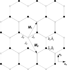
Figure 1: The honeycomb lattice. Empty (filled) circles form the sub-lattice $a$ $(b)$. The bonds with positive (negative) slope are called $x$ $(y)$ bonds. The vertical bonds are called $z$ bonds. $\mathbf{e_{x}}$ and $\mathbf{e_{y}}$ denote the unit vectors along the horizontal and the vertical directions.

We adapt the Jordan-Wigner transformation to introduce Majorana fermions $\hat{a},\hat{A}$ ($\hat{b},\hat{B}$) for sub-lattice a (b), namely,

$$\hat{a}_{j} =\left[\prod_{k<j}\sigma_{k}^{z}\right]\sigma_{j}^{y},\quad\hat{A}_{j}=\left[\prod_{k<j}\sigma_{k}^{z}\right]\sigma_{j}^{x},$$ (17)

$$\hat{b}_{j} =\left[\prod_{k<j}\sigma_{k}^{z}\right]\sigma_{j}^{x},\quad\hat{B}_{j}=\left[\prod_{k<j}\sigma_{k}^{z}\right]\sigma_{j}^{y}.$$ (18)

The product in Eqs. (17, 18) is over all sites on the one-dimensional contour which threads the entire lattice [49, 50]. It can be checked that they indeed anticommute with each other and satisfy the Majorana condition, for example,

$$\left\{\hat{a}_{j},\hat{A}_{l}\right\}=\left\{\hat{a}_{j},\hat{b}_{l}\right\}=\left\{\hat{a}_{j},\hat{B}_{l}\right\}=0,\left\{\hat{a}_{j},\hat{a}_{l}\right\}=2\delta_{jl}.$$

We rewrite the Hamiltonian in the form of Majorana fermions

$$\hat{H}=\sum_{j}i\left[J_{x}\hat{b}_{j}\hat{a}_{j-{\bf M}_{1}}+J_{y}\hat{b}_{j}\hat{a}_{j+{\bf M}_{2}}+J_{z}\hat{D}_{j}\hat{b}_{j}\hat{a}_{j}\right],$$

where the lattice vectors are ${\bf M}_{1}=\frac{\sqrt{3}}{2}{\bf e_{x}}+\frac{3}{2}{\bf e_{y}}$, ${\bf M}_{2}=\frac{\sqrt{3}}{2}{\bf e_{x}}-\frac{3}{2}{\bf e_{y}}$, and $\hat{D}_{j}\equiv-i\hat{A}_{j}\hat{B}_{j}$. It can be shown that $\hat{D}_{j}$ is a constant of motion, i.e., commutes with $\hat{H}$ [49, 50]. Since $\hat{D}_{j}^{2}=1$, $\hat{D}_{j}=\pm 1$ in its eigenspaces. According to the Lieb’s theorem [51], the ground state is in the sector with all $\hat{D}_{j}=1$; a negative $\hat{D}_{j}$ corresponds to a topological excitation [34, 49, 50]. Since we will focus on the ground state, we simply set all $\hat{D}_{j}$ to be 1. The Hamiltonian in the so-called zero-flux sector is

$$\hat{H}=\sum_{j}i\left[J_{x}\hat{b}_{j}\hat{a}_{j-{\bf M_{1}}}+J_{y}\hat{b}_{j}\hat{a}_{j+{\bf M_{2}}}+J_{z}\hat{b}_{j}\hat{a}_{j}\right].$$ (19)

Now we apply Fourier transform

$$\hat{a}_{j} =\sqrt{\frac{2}{N_{1}N_{2}}}\sum_{k\in\mathrm{HBZ}}\left(e^{ikj}\hat{a}_{k}+e^{-ikj}\hat{a}^{\dagger}_{k}\right),$$

$$\hat{b}_{j} =\sqrt{\frac{2}{N_{1}N_{2}}}\sum_{k\in\mathrm{HBZ}}\left(e^{ikj}\hat{b}_{k}+e^{-ikj}\hat{b}^{\dagger}_{k}\right),$$

with the fermionic operator $\hat{a}_{k},$ $\hat{b}_{k}$ for the $k$-th mode. The Brillouin zone (BZ) is spanned by ${\bf k}=2\pi\frac{p_{1}}{N_{1}}{\bf k}_{1}+2\pi\frac{p_{2}}{N_{2}}{\bf k}_{2},$ where $p_{1}\in\left(-\frac{N_{1}}{2},\frac{N_{1}}{2}\right),p_{2}\in\left(-\frac{N_{2}}{2},\frac{N_{2}}{2}\right)$ and ${\bf k}_{1}=\frac{1}{\sqrt{3}}{\bf e_{x}}+\frac{1}{3}{\bf e_{y}},{\bf k}_{2}=\frac{1}{\sqrt{3}}{\bf e_{x}}+\frac{-1}{3}{\bf e_{y}}$. In the above definition, we have assumed that there are $N_{1}$ empty (filled) sites in every column and $N_{2}$ in every row. And we restrict the momentum in the left half Brillouin zone (HBZ) satisfying ${\bf k}\cdot{\bf e_{x}\geq 0}$. The Hamiltonian is transformed into

$$\hat{H} =2\sum_{k\in\mathrm{HBZ}}\begin{pmatrix}\hat{a}^{\dagger}_{k}&\hat{b}^{\dagger}_{k}\end{pmatrix}\begin{pmatrix}0&-if\\ if^{*}&0\end{pmatrix}_{k}\begin{pmatrix}\hat{a}_{k}\\ \hat{b}_{k}\end{pmatrix}$$ (20)

$$=\mathrm{\frac{1}{2}}\sum_{k\in\mathrm{HBZ}}\hat{\alpha}_{k}^{T}{\mathcal{H}}_{k}\hat{\alpha}_{k},$$ (21)

where

$$\hat{\alpha}_{k}^{T}=\begin{pmatrix}\hat{a}&\hat{b}&\hat{a}^{\dagger}&\hat{b}^{\dagger}\end{pmatrix}_{k},\quad f_{k}=J_{x}e^{i{\bf k}\cdot{\bf M}_{1}}+J_{y}e^{-i{\bf k}\cdot{\bf M}_{2}}+J_{z}$$

with

$${\mathcal{H}}_{k}=2\begin{pmatrix}0&0&0&-if^{*}\\ 0&0&if&0\\ 0&-if&0&0\\ if^{*}&0&0&0\end{pmatrix}_{k}.$$ (22)

The energy spectrum is

$$E_{k} =\pm 2\sqrt{\epsilon_{k}^{2}+\Delta_{k}^{2},}$$ (23)

where

$$\epsilon_{k} =\mathrm{Re}\left[f_{k}\right]=J_{x}\cos({\bf k}\cdot{\bf M}_{1})+J_{y}\cos({\bf k}\cdot{\bf M}_{2})+J_{z},$$ (24)

$$\Delta_{k} =\mathrm{Im}\left[f_{k}\right]=J_{x}\sin({\bf k}\cdot{\bf M}_{1})-J_{y}\sin({\bf k}\cdot{\bf M}_{2}).$$ (25)

The model is gapless when $J_{x},J_{y}$ and $J_{z}$ satisfy the triangular inequality (see Fig. 2)

$$|J_{x}|\leq|J_{y}|+|J_{z}|;\quad|J_{y}|\leq|J_{x}|+|J_{z}|;\quad|J_{z}|\leq|J_{x}|+|J_{z}|.$$

We consider the following linear quench protocol,

$$J_{x}=\cos\theta,\quad J_{y}=\sin\theta,\quad J_{z}=vt,$$ (26)

where $\theta$ is fixed, and $J_{z}$ is quenched linearly from $J_{0}=vt_{0}$ to $J_{1}=vt_{1}$ with $J_{0}\ll-1$ and $J_{1}\gg 1$. The phase diagram in the plane $J_{x}+J_{y}+J_{z}=1$ and the quench protocol are shown in Fig. 2.

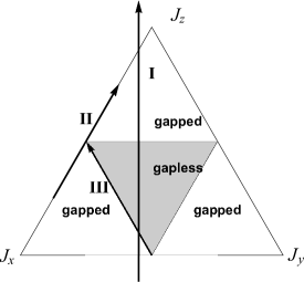
Figure 2: The phase diagram of Kitaev model in the plane $J_{x}+J_{y}+J_{z}=1$, $J_{x},J_{y},J_{z}\geq 0$. The shadowed triangle indicates the gapless phase of the KHM. The three arrows stand for three quench protocols: (I) $J_{x}=\cos(\pi/3)$, $J_{y}=\sin(\pi/3)$; (II) $\;J_{x}=1,J_{y}=0$; (III) $\;J_{x}=J_{y}+J_{z}=1.$ In all three protocols, we linearly vary $J_{z}=vt$ which starts from $J_{0}<-1$ to $J_{1}>1$.

The CFW (7) can be rewritten as

$$Z(\chi) =\mathrm{Tr}[\hat{U}^{\dagger}(t_{1},t_{0})e^{i\chi\hat{H}(t_{1})}\hat{U}(t_{1},t_{0})e^{-i\chi\hat{H}(t_{1})}\hat{\rho}_{0}]$$

$$=\mathrm{Tr}[e^{i\chi\hat{H}^{H}(t_{1})}e^{-(i\chi+\beta)\hat{H}(t_{0})}],$$

where

$$\hat{H}^{H}(t_{1}) =\hat{U}^{\dagger}(t_{1},t_{0})\hat{H}(t_{1})\hat{U}(t_{1},t_{0})$$

$$=\sum_{k\in\mathrm{HBZ}}\hat{\alpha}_{k}^{T}(t_{1}){\mathcal{H}}_{k}(t_{1})\hat{\alpha}_{k}(t_{1})$$ (27)

is the final Hamiltonian in the Heisenberg picture, and the ground state is represented by a thermal equilibrium state $\hat{\rho}_{0}=e^{-\beta\hat{H}(t_{0})}/\mathrm{Tr}[e^{-\beta\hat{H}(t_{0})}]$ with $\beta\to\infty$. $\hat{\alpha}_{k}(t_{1})$ is determined by the Heisenberg equation of motion

$$i\frac{d}{dt}\hat{\alpha}_{k}^{H}(t)=\left[\hat{\alpha}_{k}^{H},\hat{H}^{H}(t)\right].$$

The solution is linear due to the quadratic form of the Hamiltonian

$$\hat{\alpha}_{k}^{H}(t)=L_{k}(t)\hat{\alpha}_{k}+C_{k}(t).$$

where the coefficient matrices $L_{k}(t)$ and $C_{k}(t)$ satisfy

$$i\frac{d}{dt}L_{k}(t) =\tau_{F}{\mathcal{H}}_{k}(t)L_{k}(t),\quad L(t_{0})={\bf I}_{4\times 4},$$

$$i\frac{d}{dt}C_{k}(t) =\tau_{F}{\mathcal{H}}_{k}(t)C_{k}(t),\quad C(t_{0})=0,$$ (28)

with

$$\tau_{F}=\begin{pmatrix}0&{\bf I}_{2\times 2}\\ {\bf I}_{2\times 2}&0\end{pmatrix}$$

and ${\bf I}_{n\times n}$ is the $n$-dimensional identity matrix. The dynamics is mapped to the standard Landau-Zener problem [30]. We find $C_{k}(t_{1})=0$, and the transition matrix $L_{k}(t_{1})=\mathrm{diag}(\Lambda_{k},\Lambda_{k}^{*})$ is a block diagonal matrix where the $2\times 2$ matrix $\Lambda_{k}$ in the limit $t_{0}\to-\infty$, $t_{1}\to\infty$ is

$$\small\Lambda_{k}(t_{1}) \approx\sqrt{p_{k}}\left[\cos\Theta_{k}(t_{1},t_{0}){\bf I}_{2\times 2}+i\sin\Theta_{k}(t_{1},t_{0})\sigma^{y}\right]$$

$$\quad-i\sqrt{1-p_{k}}\left[\cos\Theta^{\prime}_{k}(t_{1},t_{0})\sigma^{z}-\sin\Theta^{\prime}_{k}(t_{1},t_{0})\sigma^{x}\right],$$ (29)

where $\Theta(t_{1},t_{0})$ and $\Theta^{\prime}(t_{1},t_{0})$ are two phase factors which do not appear in the final result of the CFW in the above limits. For completeness, we give the expression of $\Theta(t_{1},t_{0})$ and $\Theta^{\prime}(t_{1},t_{0})$ in Appendix A. The Landau-Zener transition probability $p_{k}$ for mode $k$ is

$$p_{k}=e^{-\frac{2\pi}{v}\Delta_{k}^{2}}=e^{-\frac{2\pi}{v}\left[J_{x}\sin({\bf k}\cdot{\bf M}_{1})-J_{y}\sin({\bf k}\cdot{\bf M}_{2})\right]^{2}}.$$ (30)

Substituting these results into Eq. (27), the Hamiltonian at the final time can be written as

$$\hat{H}^{H}(t_{1}) =\sum_{k\in\mathrm{HBZ}}\hat{\alpha}_{k}^{T}(t_{1}){\mathcal{H}}_{k}(t_{1})\hat{\alpha}_{k}(t_{1})$$

$$=\sum_{k\in\mathrm{HBZ}}\hat{\alpha}_{k}^{T}L_{k}^{T}(t_{1}){\mathcal{H}}_{k}(t_{1})L_{k}(t_{1})\hat{\alpha}_{k}.$$

Now we use the trace formula [48]

$$\small\mathrm{Tr}\left[\prod_{k}\exp\left(\mathrm{\frac{1}{2}}\hat{\alpha}_{k}^{T}{\mathcal{H}}_{k}\hat{\alpha}_{k}\right)\right]=\left\{\det\left[\prod_{k}\exp\left(\tau_{F}{\mathcal{H}}_{k}\right)+I\right]\right\}^{\frac{1}{2}}$$ (31)

and find that the CFW at zero temperature can be approximately (exactly in the limit $t_{0}\to-\infty,$ $t_{1}\to\infty$) written as

$$Z(\chi) =\prod_{k}Z(\chi,k)$$

$$=e^{-2i(J_{1}+J_{0})\chi}\prod_{k}\left[(1-p_{k})+p_{k}e^{4iJ_{1}\chi}\right].$$ (32)

We see that the CFW consists of two parts: a global work corresponding to the shift of zero-point energy (the ground state energies are $2J_{0}$ and $-2J_{1}$ at the initial time $t_{0}$ and the final time $t_{1}$, respectively); a product of contributions from different $k$ modes. For every $k$ mode, there is a probability $p_{k}$ of exciting a quasiparticle at the cost of work $4J_{1}$. The CGF can be expressed as

$${\mathcal{G}}(\chi) =\frac{1}{N}\ln Z(\chi)=\int_{\mathrm{HBZ}}\frac{d^{2}k}{S_{\mathrm{BZ}}}\ln Z(k,\chi)$$

$$\approx\int_{\mathrm{HBZ}}\frac{d^{2}k}{S_{\mathrm{BZ}}}\left[\ln\left(1-p_{k}+p_{k}e^{4iJ_{1}\chi}\right)-2i\chi(J_{0}+J_{1})\right],$$ (33)

where $S_{\mathrm{BZ}}$ is the area of the BZ. As mentioned before, the second term in Eq. (33) only shifts the mean value of work $\kappa_{1}$ by a constant, and does not affect higher-order cumulants $\kappa_{n}\;(n\geq 2)$. So we can ignore it in $\kappa_{1}$ in the analysis of the scaling behavior. Substituting Eq. (30) into Eq. (33), we obtain the scaling behavior of the first three cumulants

$$\kappa_{1} =\int_{\mathrm{HBZ}}\frac{d^{2}k}{S_{\mathrm{BZ}}}4J_{1}p_{k}\sim v^{1/2},$$

$$\kappa_{2} =\int_{\mathrm{HBZ}}\frac{d^{2}k}{S_{\mathrm{BZ}}}(4J_{1})^{2}p_{k}(1-p_{k})\sim v^{1/2},$$

$$\kappa_{3} =\int_{\mathrm{HBZ}}\frac{d^{2}k}{S_{\mathrm{BZ}}}(4J_{1})^{3}p_{k}(1-p_{k})(1-2p_{k})\sim v^{1/2},$$ (34)

which are consistent with Eq. (15) with $m=\nu=z=1$ for the KHM. Higher-order cumulants of work can be obtained in a similar way.

In the following, we consider two quench protocols (a third protocol that quenches along one edge of the gapless phase is left in Appendix B). Although they all lead to the same scaling behaviors, the details differ. In protocol I, we choose $\theta=\pi/3$ [see Fig. 2 (I)]. The system crosses through the gapless phase without touching any vertexes of the shaded triangle in Fig. 2. Corresponding to any points in the gapless phase, there are some isolated Fermi points in the HBZ for which the gap vanishes. As $J_{z}$ ramps up, these isolated Fermi points draw critical lines in the HBZ. In protocol II, $\theta=0$ [see Fig. 2 (II)], we quench the system along one edge of the big triangle in Fig. 2. In this protocol, only one (multi)critical point is touched. At this (multi)critical point, the gap vanishes along a line (instead of some isolated points) in the HBZ. Now we numerically integrate the time-dependent Schr$\ddot{\mathrm{o}}$dinger equations in momentum space, and show the simulation results of cumulants of work statistics in Fig. 3. It can be seen that the numerical results agree very well with our theoretical prediction.

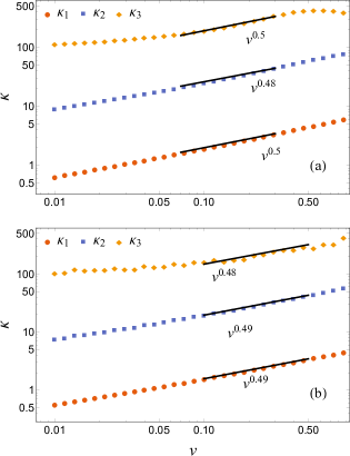
Figure 3: The first three cumulants of work for the KHM quenched linearly across a gapless phase. The parameters are chosen to be $J_{1}=10,J_{0}=-10$, $\theta=\pi/3$ for (a) and $\theta=0$ for (b). The markers correspond to the results from numerical integration of the time-dependent Schr$\ddot{\mathrm{o}}$dinger equations in momentum space and solid lines are the fits. The site number is $400\times 400$. The slopes of the solid lines are in good agreement with the theoretical prediction (15).

IV Discussion And Summary

Before concluding our article, we would like to give the following remarks: (1) We consider the scaling behavior of the cumulants of the work distribution only. In parallel, the scaling behavior of the cumulants of the topological defects can be studied in a similar way. In fact, they exhibit exactly the same scaling behaviors. (2) The critical surface can be easily found in a wide range of models. It either has a gapless phase while the gap vanishes in a handful of isolated points in the BZ, or it has single critical point but the gap vanishes at a surface in the BZ. The above two features are expected in high dimensional or multiple parameter-dependent systems, such as the nodal line semimetal [52, 53, 54]. An trivial example of the first case is the 1D Kitaev chain (or 1D XY model) [55, 56], which has gapless phase when the superconducting gap is zero. When quenching across this gapless phase, the gapless point sweeps the 1D BZ, forming a 1D critical surface. The work and quasiparticle excitation are all constant, consistent with the prediction of Eq. (15). (3) We consider only the situation of quenching the system from one gapped phase to another. Other protocols can also be considered such as stopping at an anisotropic QCP [23] or periodically driven protocols [57]. Hopefully, different scaling behaviors of cumulants of work will be obtained for these protocols.

In summary, we have extended the scaling behavior for work statistics form crossing an isolated QCP to a critical surface. The presence of the critical surface reduces the available phase space for quasiparticle excitation, resulting in a scaling behavior for work statistics different from the situation of an isolated QCP. We use the adiabatic perturbation theory to study the general scaling behavior and calculate the exact CFW of the KHM by utilizing the group-theoretical technique to verify our general results. The exact CFW shows that the work distribution is a Poisson binomial distribution. Extensions of our current work to systems beyond the quasiparticle picture and single-particle excitation approximation will be given in our future studies.

Appendix A Landau-Zener Problem of KHM

In this appendix, we sketch the solution to Eq. (28). Since $\tau_{F}{\mathcal{H}}_{k}$ in Eq. (28) is block diagonal, $L_{k}(t)$ and $C_{k}(t)$ will remain block diagonal in the evolution as they are initially block diagonal. We do not need to consider $C_{k}(t)$, because $C_{k}(t)$ is a zero matrix initially and will remain zero under the unitary evolution. It is sufficient to consider the evolution of the upper block matrix $\Lambda_{k}(t)$ of $L_{k}(t)$. The lower block matrix is related to the upper block matrix by the complex conjugate. The upper block matrix of $\tau_{F}{\mathcal{H}}_{k}$ is

$${\mathcal{H}}_{k}^{u}=\begin{pmatrix}0&-if\\ if^{*}&0\end{pmatrix}_{k}=\epsilon_{k}\sigma^{y}+\Delta_{k}\sigma^{x}.$$ (35)

The dynamics can be transformed to the standard form of the Landau-Zener problem by a gauge transformation $U_{x}=\exp(-i\pi\sigma^{x}/4)$ and introducing a rescaled time $s_{k}=\sqrt{2v}t+\sqrt{2}(J_{x}\cos k_{1}+J_{y}\cos k_{2})/v$ [25, 33, 23]. For simplicity, we omit the subscript $k$ of $s_{k}$. The equation of motion of $\tilde{\Lambda}_{k}(s)=U_{x}\Lambda_{k}(t)$ is

$$i\frac{d}{ds}\tilde{\Lambda}_{k}(s)=\begin{pmatrix}s&\sqrt{2}\Delta_{k}/\sqrt{v}\\ \sqrt{2}\Delta_{k}/\sqrt{v}&s\end{pmatrix}\Lambda_{k}^{\prime}.$$

In the limit $t_{0}\to-\infty,t_{1}\to\infty$, i.e., $s_{0}\equiv s(t_{0})\to-\infty,s_{1}\equiv s(t_{1})\to\infty,$ the asymptotic solution of $\tilde{\Lambda}_{k}(s)$ is

$$\tilde{\Lambda}_{k}(s_{1})=\bigg{\{}\sqrt{p_{k}}\left[\cos\tilde{\Theta}_{k}(s_{1},s_{0}){\bf I}_{2\times 2}+i\sin\tilde{\Theta}_{k}(s_{1},s_{0})\sigma^{z}\right]+i\sqrt{1-p_{k}}\left[\cos\tilde{\Theta^{\prime}}_{k}(s_{1},s_{0})\sigma^{y}+\sin\tilde{\Theta^{\prime}}_{k}(s_{1},s_{0})\sigma^{x}\right]\bigg{\}}\tilde{\Lambda}_{k}(s_{0}),$$

where $\tilde{\Lambda}_{k}(s_{0})=U_{x}$, Landau-Zener transition probability $p_{k}=\exp(-2\pi\Delta_{k}^{2}/v)$ and

$$\tilde{\Theta}(s_{1},s_{0}) =-\frac{i}{2}(s_{1}^{2}-s_{0}^{2})+\frac{i\Delta_{k}^{2}}{v}\ln(-s_{0}/s_{1}),$$

$$\tilde{\Theta}^{\prime}(s_{1},s_{0}) =i\pi/4-\frac{i}{2}(s_{1}^{2}+s_{0}^{2})-\frac{i\Delta_{k}^{2}}{v}\ln(-2s_{0}s_{1})+\ln\left[\Gamma(i\Delta_{k}^{2}/v)\sqrt{\Delta_{k}^{2}\sinh(\pi\Delta_{k}^{2}/v)/(v\pi)}\right]$$ (36)

with gamma function $\Gamma(x)$. Changing the variable from $s$ to $t$ in Eq. (36), we obtain the expression of $\Theta(t_{1},t_{0})$ and $\Theta^{\prime}(t_{1},t_{0})$ in Eq. (29).

Appendix B Quench along one edge of the gapless phase

In this appendix, we consider the protocol that quenches along one edge of the shaded triangle [see Fig. 2 (III)], i.e. we keep $J_{x}=J_{y}+J_{z}$ and linearly vary $J_{z}=vt$ and $J_{y}=J_{x}-vt.$ The system is always gapless along the edge. The Hamiltonian of the corresponding Landau-Zener problem is

$$\hat{H}_{LZ}({\bf k})=2\left[vt\sin\frac{k_{2}}{2}+\tilde{\epsilon}({\bf k})\right]\hat{\sigma}_{z}+2\tilde{\Delta}({\bf k})\hat{\sigma}_{\perp}({\bf k}),$$

where $\tilde{\epsilon}({\bf k})=2J_{x}\sin[(2k_{2}-k_{1})/2]\cos[(k_{1}+k_{2})]/2,$ and the minimum gap $2\tilde{\Delta}({\bf k})=2J_{x}\cos[(k_{1}-2k_{2})/2]\cos\left[\left(k_{1}+k_{2}\right)/2\right].$ The matrix $\hat{\sigma}_{\perp}({\bf k})=-\sin\left(k_{2}/2\right)\hat{\sigma}_{x}+\cos\left(k_{2}/2\right)\hat{\sigma}_{y}.$ The Landau-Zener probability for this protocol is

$$p_{k}^{\prime} =\exp\left[-\frac{2\pi\tilde{\Delta}^{2}({\bf k})}{v\sin(k_{2}/2)}\right]$$

$$=\exp\left[-\frac{8\pi J_{x}^{2}\cos^{2}\left(\frac{k_{1}-2k_{2}}{2}\right)\cos^{2}\left(\frac{k_{1}+k_{2}}{2}\right)}{v\sin(k_{2}/2)}\right].$$

Corresponding to this protocol, there are three critical lines in which the minimum gap $\tilde{\Delta}$ vanishes: $k_{x}=\pi/\sqrt{3}$, $k_{x}=3\sqrt{3}k_{y}\pm 2\pi/\sqrt{3}.$ Expand $\tilde{\Delta}({\bf k})$ along these critical lines, we get $\tilde{\Delta}({\bf k})\sim|{\bf k}|\equiv|{\bf k}|^{z_{2}}$ and $\tilde{\epsilon}({\bf k})\sim|{\bf k}|^{2}\equiv|{\bf k}|^{z_{1}}$. Hence, the dynamical critical exponent is still $z=1$. Since this protocol also draws critical lines in the HBZ, we conclude that its scaling behavior of work statistics is the same as quenching across the inner area of the gapless phase, i.e., $\kappa_{n}\sim v^{1/2}.$ This is different from the case in 1D XY model when quenching along the gapless line [55, 56, 58], where $z=z_{1}=1<z_{2}=2$. In the latter case, the mean density of defects scales as $\left\langle n_{ex}\right\rangle\sim v^{d\nu/(\nu z_{2}+1)}=v^{1/3}$ rather than $v^{d\nu/(z\nu+1)}=v^{1/2}$ predicted by KZM.

References

- Bloch et al. [2008] I. Bloch, J. Dalibard, and W. Zwerger, Rev. Mod. Phys. 80, 885 (2008).
- Dziarmaga [2010] J. Dziarmaga, Adv. Phys. 59, 1063 (2010).
- Cazalilla et al. [2011] M. A. Cazalilla, R. Citro, T. Giamarchi, E. Orignac, and M. Rigol, Rev. Mod. Phys. 83, 1405 (2011).
- Polkovnikov et al. [2011] A. Polkovnikov, K. Sengupta, A. Silva, and M. Vengalattore, Rev. Mod. Phys. 83, 863 (2011).
- Altman and Vosk [2015] E. Altman and R. Vosk, Annu. Rev. Condens. Matter Phys. 6, 383 (2015).
- Langen et al. [2015] T. Langen, R. Geiger, and J. Schmiedmayer, Annu. Rev. Condens. Matter Phys. 6, 201 (2015).
- Aoki et al. [2014] H. Aoki, N. Tsuji, M. Eckstein, M. Kollar, T. Oka, and P. Werner, Rev. Mod. Phys. 86, 779 (2014).
- Heyl [2018] M. Heyl, Rep. Prog. Phys. 81, 054001 (2018).
- Monroe et al. [2021] C. Monroe, W. C. Campbell, L.-M. Duan, Z.-X. Gong, A. V. Gorshkov, P. W. Hess, R. Islam, K. Kim, N. M. Linke, G. Pagano, P. Richerme, C. Senko, and N. Y. Yao, Rev. Mod. Phys. 93, 025001 (2021).
- Kibble [1976] T. W. B. Kibble, J. Phys. A 9, 1387 (1976).
- Kibble [1980] T. Kibble, Phys. Rep. 67, 183 (1980).
- Zurek [1985] W. H. Zurek, Nature 317, 505 (1985).
- Zurek [1996] W. Zurek, Phys. Rep. 276, 177 (1996).
- Sachdev [2011] S. Sachdev, Quantum phase transitions (Cambridge university press, 2011).
- Dziarmaga [2005] J. Dziarmaga, Phys. Rev. Lett. 95, 245701 (2005).
- Polkovnikov [2005] A. Polkovnikov, Phys. Rev. B 72, 161201(R) (2005).
- Zurek et al. [2005] W. H. Zurek, U. Dorner, and P. Zoller, Phys. Rev. Lett. 95, 105701 (2005).
- Polkovnikov [2008] A. Polkovnikov, Phys. Rev. Lett. 101, 220402 (2008).
- Sengupta and Sen [2009] K. Sengupta and D. Sen, Phys. Rev. A 80, 032304 (2009).
- Sen et al. [2008] D. Sen, K. Sengupta, and S. Mondal, Phys. Rev. Lett. 101, 016806 (2008).
- Barankov and Polkovnikov [2008] R. Barankov and A. Polkovnikov, Phys. Rev. Lett. 101, 076801 (2008).
- Dutta et al. [2010] A. Dutta, R. R. P. Singh, and U. Divakaran, Europhys. Lett. 89, 67001 (2010).
- Hikichi et al. [2010] T. Hikichi, S. Suzuki, and K. Sengupta, Phys. Rev. B 82, 174305 (2010).
- Mukherjee and Dutta [2010] V. Mukherjee and A. Dutta, Europhys. Lett. 92, 37004 (2010).
- Sengupta et al. [2008] K. Sengupta, D. Sen, and S. Mondal, Phys. Rev. Lett. 100, 077204 (2008).
- Polkovnikov and Gritsev [2008] A. Polkovnikov and V. Gritsev, Nat. Phys. 4, 477 (2008).
- del Campo [2018] A. del Campo, Phys. Rev. Lett. 121, 200601 (2018).
- Gómez-Ruiz et al. [2020] F. J. Gómez-Ruiz, J. J. Mayo, and A. del Campo, Phys. Rev. Lett. 124, 240602 (2020).
- Fei et al. [2020] Z. Fei, N. Freitas, V. Cavina, H. T. Quan, and M. Esposito, Phys. Rev. Lett. 124, 170603 (2020).
- De Grandi and Polkovnikov [2010] C. De Grandi and A. Polkovnikov, in Quantum Quenching, Annealing and Computation (Springer, 2010) pp. 75–114.
- Halperin [2019] B. I. Halperin, Phys. Today 72, 42 (2019).
- Note [1] For the fermionic quasiparticle, it is always satisfied, while for bosonic excitation, this approximation is fulfilled only for small excitation probability.
- Mondal et al. [2008] S. Mondal, D. Sen, and K. Sengupta, Phys. Rev. B 78, 045101 (2008).
- Kitaev [2006] A. Kitaev, Ann. Phys. 321, 2 (2006).
- Trebst [2017] S. Trebst, arXiv:1701.07056 (2017).
- Zhou et al. [2017] Y. Zhou, K. Kanoda, and T.-K. Ng, Rev. Mod. Phys. 89, 025003 (2017).
- Takagi et al. [2019] H. Takagi, T. Takayama, G. Jackeli, G. Khaliullin, and S. E. Nagler, Nat. Rev. Phys. 1, 264 (2019).
- Broholm et al. [2020] C. Broholm, R. J. Cava, S. A. Kivelson, D. G. Nocera, M. R. Norman, and T. Senthil, Science 367, 6475 (2020).
- Sandilands et al. [2015] L. J. Sandilands, Y. Tian, K. W. Plumb, Y.-J. Kim, and K. S. Burch, Phys. Rev. Lett. 114, 147201 (2015).
- Banerjee et al. [2016] A. Banerjee, C. A. Bridges, J.-Q. Yan, A. A. Aczel, L. Li, M. B. Stone, G. E. Granroth, M. D. Lumsden, Y. Yiu, J. Knolle, S. Bhattacharjee, D. L. Kovrizhin, R. Moessner, D. A. Tennant, D. G. Mandrus, and S. E. Nagler, Nat. Mater. 15, 733 (2016).
- Do et al. [2017] S.-H. Do, S.-Y. Park, J. Yoshitake, J. Nasu, Y. Motome, Y. Kwon, D. T. Adroja, D. J. Voneshen, K. Kim, T.-H. Jang, J.-H. Park, K.-Y. Choi, and S. Ji, Nat. Phys. 13, 1079 (2017).
- Zheng et al. [2017] J. Zheng, K. Ran, T. Li, J. Wang, P. Wang, B. Liu, Z.-X. Liu, B. Normand, J. Wen, and W. Yu, Phys. Rev. Lett. 119, 227208 (2017).
- Baek et al. [2017] S.-H. Baek, S.-H. Do, K.-Y. Choi, Y. S. Kwon, A. U. B. Wolter, S. Nishimoto, J. van den Brink, and B. Büchner, Phys. Rev. Lett. 119, 037201 (2017).
- Manni et al. [2014] S. Manni, S. Choi, I. I. Mazin, R. Coldea, M. Altmeyer, H. O. Jeschke, R. Valentí, and P. Gegenwart, Phys. Rev. B 89, 245113 (2014).
- Hwan Chun et al. [2015] S. Hwan Chun, J.-W. Kim, J. Kim, H. Zheng, C. Stoumpos, C. Â. D. Malliakas, J. Â. F. Mitchell, K. Mehlawat, Y. Singh, Y. Choi, T. Gog, A. Al-Zein, M. Sala, M. Krisch, J. Chaloupka, G. Jackeli, G. Khaliullin, and B. J. Kim, Nat. Phys. 11, 462 (2015).
- Das et al. [2019] S. D. Das, S. Kundu, Z. Zhu, E. Mun, R. D. McDonald, G. Li, L. Balicas, A. McCollam, G. Cao, J. G. Rau, H.-Y. Kee, V. Tripathi, and S. E. Sebastian, Phys. Rev. B 99, 081101(R) (2019).
- Patel and Dutta [2012] A. A. Patel and A. Dutta, Phys. Rev. B 86, 174306 (2012).
- Fei and Quan [2019] Z. Fei and H. T. Quan, Phys. Rev. Research 1, 033175 (2019).
- Feng et al. [2007] X.-Y. Feng, G.-M. Zhang, and T. Xiang, Phys. Rev. Lett. 98, 087204 (2007).
- Chen and Nussinov [2008] H.-D. Chen and Z. Nussinov, J. Phys. A 41, 075001 (2008).
- Lieb [1994] E. H. Lieb, Phys. Rev. Lett. 73, 2158 (1994).
- Xie et al. [2015] L. S. Xie, L. M. Schoop, E. M. Seibel, Q. D. Gibson, W. Xie, and R. J. Cava, APL Materials 3, 083602 (2015), https://doi.org/10.1063/1.4926545 .
- Chan et al. [2016] Y.-H. Chan, C.-K. Chiu, M. Y. Chou, and A. P. Schnyder, Phys. Rev. B 93, 205132 (2016).
- Wang and Nandkishore [2017] Y. Wang and R. M. Nandkishore, Phys. Rev. B 95, 060506(R) (2017).
- Divakaran et al. [2009] U. Divakaran, V. Mukherjee, A. Dutta, and D. Sen, 2009, P02007 (2009).
- Deng et al. [2009] S. Deng, G. Ortiz, and L. Viola, Phys. Rev. B 80, 241109(R) (2009).
- Dutta et al. [2015] A. Dutta, A. Das, and K. Sengupta, Phys. Rev. E 92, 012104 (2015).
- Mondal et al. [2009] S. Mondal, K. Sengupta, and D. Sen, Phys. Rev. B 79, 045128 (2009).