BDD-Based Algorithm for SCC Decomposition
of Edge-Coloured Graphs

Abstract.

Edge-coloured directed graphs provide an essential structure for modelling and analysis of complex systems arising in many scientific disciplines (e.g. feature-oriented systems, gene regulatory networks, etc.). One of the fundamental problems for edge-coloured graphs is the detection of strongly connected components, or SCCs.

The size of edge-coloured graphs appearing in practice can be enormous both in the number of vertices and colours. The large number of vertices prevents us from analysing such graphs using explicit SCC detection algorithms, such as Tarjan’s, which motivates the use of a symbolic approach. However, the large number of colours also renders existing symbolic SCC detection algorithms impractical.

This paper proposes a novel algorithm that symbolically computes all the monochromatic strongly connected components of an edge-coloured graph. In the worst case, the algorithm performs $O(p\cdot n\cdot\log n)$ symbolic steps, where $p$ is the number of colours and $n$ is the number of vertices.

We evaluate the algorithm using an experimental implementation based on binary decision diagrams (BDDs). Specifically, we use our implementation to explore the SCCs of a large collection of coloured graphs (up to $2^{48}$) obtained from Boolean networks – a modelling framework commonly appearing in systems biology.

Introduction

In many scientific disciplines, the processing of massive data sets represents one of the most important computational tasks. A variety of these data sets can be modelled in terms of very large multi-graphs, augmented by a specific collection of application-dependent edge attributes. These attributes are often abstractly referred to as colours, and the resulting formalism is called an edge-coloured graph [BJG97, BCLF79]. Geographic information systems, telecommunications traffic, or internet networks are prime examples of data that are best represented as such edge-coloured graphs.

For instance, in social networks, coloured edges can be used to link together groups of nodes related by some specific criteria (Sports, Health, Technology, Religion, etc.). In software engineering, one often speaks about feature-oriented systems [CHS⁺10]. In this case, colours represent possible combinations of features, altering the system’s behaviour.

Our interest in processing huge edge-coloured graphs is primarily motivated by applications taken from systems biology [BBK⁺12, GGG⁺17] and genetics [Dor94] where we have to deal not only with giant graphs as measured by the number of vertices and edges but also with large sets of colours. In this case, the graph colours represent valuations of numerous parameters that influence the dynamics of a biological system [BBK⁺12, BPC⁺10, RCB05].

Fundamental graph algorithms such as breadth-first search, spanning tree construction, shortest paths, decomposition into strongly connected components (SCCs), etc., are building blocks of many practical applications. For the edge-coloured graphs, the primary research focus so far has been on some of the “classical” coloured graph problems, like the determination of the chromatic index, finding sub-graphs with a specified colour property (the coloured version of the k-linked problem), alternating edge-coloured cycles and paths, rainbow cliques, monochromatic cliques and cycles, etc. [ADF⁺08, AA07, AG97, BJG97, TW07, KL08].

To the best of our knowledge, we are not aware of any work on SCC decomposition specifically for edge-coloured graphs, even though this problem has many important applications. For example, in biological systems, strongly connected components represent the so called attractors of the system. In this case, a specific focus is given to terminal (or bottom) SCCs, but non-terminal (transient) SCCs can also be detrimental to the system’s long-term behaviour [PIS⁺21]. Overall, SCCs play an essential role in determining the system’s biological properties, since they may correspond, for example, to the specific phenotypes expressed by a cell [CC16].

The valuation of parameters (e.g. the presence of certain genes or external stimuli) in such systems is then represented as edge colours in the state-transition graph. The knowledge of SCCs and how their structure depends on parameters is vital for understanding various biological phenomena [DAERR16, LWA⁺16]. Other applications where investigation of attractors is crucial include predictions of the global climate change [SRR⁺18] or predictions of spreading of infectious diseases such as COVID-19 [Mat20].

There is a serious computational problem related to the processing of massive edge-coloured graphs (or even the non-coloured ones) that significantly affects the tractability of SCC decomposition. The graphs often cannot be handled using standard (explicit) representations, since they are too large to be kept in the main memory. Various approaches have been considered to deal with such giant graphs: distributed-memory computation, symbolic data structures for graph representation, or storing the graphs in external memory. We review these approaches in more detail in the related work section.

In [BBB⁺17, BBP⁺19] we have initially attacked the SCC decomposition problem for massive edge-coloured graphs by developing a parallel, semi-symbolic algorithm for detection of bottom SCCs. The algorithm uses symbolic structures to represent sets of parameters, while the graph itself is represented explicitly. However, the results have shown that the parallel semi-symbolic algorithm is often not sufficient to tackle graphs representing real-world problems practically. These findings have motivated us to propose a new, entirely symbolic approach.

In this paper, we consider edge-coloured multi-digraphs, i.e., multi-digraphs such that each directed edge has a colour and no two parallel (i.e., joining the same pair of vertices) edges have the same colour. Here, we refer to such graphs simply as coloured graphs. For coloured graphs, we can define several notions of strongly connected components involving colours. We consider the simplest case, where the SCCs are monochromatic, that is all their edges have the same colour [Kir14]. This choice is motivated by the application in systems biology, as mentioned above.

Contribution

We propose a novel fully symbolic algorithm for detecting all monochromatic strongly connected components in a coloured graph. This algorithm is in practice significantly faster than what is achievable by naïvely executing a symbolic SCC decomposition algorithm for each colour separately. This is because in many applications, the edges are largely shared among individual colours [BBK⁺12] and our algorithm is capable of exploiting this fact. The algorithm conceptually follows the lock-step reachability approach by Bloem et al. [BGS00] for purely monochromatic digraphs. The key new ingredients behind our algorithm are a careful orchestration of the forward and backward reachability for different colours, and a colour-aware selection of the pivot set.

Structure of the paper

In Section 1, we recall the notions of strongly connected components and edge-coloured digraphs, and we state the coloured SCC decomposition problem. In Section 2, we first briefly introduce the forward-backward decomposition algorithm and the lock-step algorithm for monochromatic graphs. After that, we present the coloured SCC decomposition algorithm together with the proof of correctness and complexity analysis.

In Section 3, we introduce Boolean networks, discuss their symbolic encoding, and show how they can be translated into coloured graphs suitable for SCC-decomposition. Subsequently, Section 4 discusses several practical improvements to the main algorithm (saturation, trimming, and parallelism) which help it scale to larger models, and thus be more practically viable. Finally, Section 4 evaluates the main algorithm (including the improved variants) using a collection of large, real-world Boolean networks. A conclusion is provided in the last section.

This article is an extended version of an article that appeared in the Proceedings of TACAS 2021 [BBPŠ21]. We extend the information provided in the TACAS Proceedings with more in-depth technical details of the algorithm and related proof, including explanation of its key steps. Moreover, we extend the implementation and evaluation sections to give the reader more information on how the performance of the algorithm can be improved, and how the algorithm performs using a variety of real-world case studies.

Related Work

The detection of SCCs in (monochromatic) digraphs is a well-known problem computable in linear time. Best serial (explicit) algorithms are Kosaraju-Sharir [Sha81] and Tarjan [Tar72], which are both inherently based on depth-first search. However, these algorithms do not scale for large graphs, e.g., those encountered in model-checking, when using explicit graph representation. Therefore, alternative approaches to such SCC decomposition have been proposed (e.g. I/O efficient, parallel, or symbolic algorithms).

The algorithm of Jiang [Jia93] gives an I/O-efficient alternative based on a combination of depth-first and breadth-first search.

Efficient parallel, distributed-memory algorithms avoid the inherently sequential DFS step [Rei85] in several different ways. The Forward-Backward algorithm [FHP00] employs a divide-and-conquer approach relying on picking a pivot state and splitting the graph in three independent (SCC-closed) parts. The approach of Orzan [Orz05] uses a different distribution scheme called a colouring transformation, employing a set of prioritised colours to split the graph into many parts at once. The OWCTY-Backward-Forward (OBF) approach is proposed in [BCVDP11]. It recursively splits the graph in a number of independent sub-graphs called OBF slices and applies to each slice the One-Way-Catch-Them-Young (OWCTY) technique. In [SRM14], the authors utilise variants of the Forward-Backward and Orzan’s algorithms for optimal execution on shared-memory multi-core platforms. Finally, Bloemen et al. [BLvdP16] present an on-the-fly parallel algorithm utilising a swarm of DFS searches, showing promising speed-up for large graphs containing large SCCs. On another end, GPU-accelerated approaches to computing SCCs have been addressed for example in [BBBv11, HRO13, LZCY14, WKB14].

Computing SCCs of (monochromatic) digraphs symbolically is another way to handle giant graphs and has been thoroughly explored in literature. As in the case of efficient parallelisation, depth-first search is not feasible in the symbolic framework [GPP08]. In consequence, many DFS-based algorithms cannot be easily revised to work with symbolically represented graphs. An algorithm based on forward and backward reachability performing $\mathcal{O}(n^{2})$ symbolic steps was presented by Xie and Beerel in [XB00]. Bloem et al. present an improved $\mathcal{O}(n\cdot\log n)$ algorithm in [BGS00]. Finally, an $\mathcal{O}(n)$ algorithm was presented by Gentilini et al. in [GPP03, GPP08]. This bound has been proven to be tight in [CDHL18]. In [CDHL18], the authors argue that the algorithm from [GPP03] is optimal even when considering more fine-grained complexity criteria, like the diameter of the graph and the diameters of the individual components. Ciardo et al. [ZC11] use the idea of saturation [CMS06] to speed up state exploration within the Xie-Beerel algorithm, and show a saturation-based technique for computing the transitive closure of the graph’s edge relation.

Besides these generic algorithms, there have also been symbolic SCC decomposition methods to deal with large graphs generated specifically by Boolean networks [MPQY19, YMPQ19]. However, these primarily target detection of bottom SCCs. Methods in this area are also often incomplete, for example focusing on detection of single-state or small bottom SCCs [ZHA⁺07]. As such, they generally perform better than an exhaustive symbolic SCC detection in their respective application domains, but are inherently limited in scope.

1. Problem Definition

As we have already stated in the introductory section, the SCC decomposition problem for edge-coloured graphs has remained mostly unexplored until now. We thus start this paper by introducing and formalising the notion of coloured SCC decomposition itself and state some of its basic properties.

Before giving exact definitions, it might be instructive to discuss the substance of the coloured SCC decomposition intuitively. There are several ways of capturing the notion of a “coloured connected component”. One of them is that of a colour-connectivity first introduced by Saad [Saa92]. It is based on alternating paths in which successive edges differ in colour. However, there is no unique, universally acceptable notion of a coloured component.

In the biological applications we have in mind (i.e. Boolean networks), we want to identify a coloured component as a coloured collection of SCCs—a collection where for every colour there is a set of all relevant monochromatic SCCs. Such a setting leads us to represent SCCs in the form of a relation. To that end, we first introduce such a relation for monochromatic graphs (Section 1.1) and afterwards extend it to edge-coloured graphs (Section 1.2). The relation-based approach gives us also the advantage of allowing a feasible symbolic encoding of the problem.

1.1. Graphs and Strongly Connected Components

Let us first recall the standard definitions of a directed graph and its strongly connected components:

A directed graph is a tuple $G=(V,E)$ where $V$ is a set of graph vertices and $E\subseteq V\times V$ is a set of graph edges.

We are going to use the word graph to mean directed graph in the following. We write $u\to v$ when $(u,v)\in E$ and $u\to^{*}v$ when $(u,v)\in E^{*}$, the reflexive and transitive closure of $E$. We say that $v$ is reachable from $u$ if $u\to^{*}v$. The reachability relation allows us to decompose a graph into strongly connected components, defined as follows:

In a graph $G=(V,E)$, a strongly connected component (SCC) is a maximal set $W\subseteq V$ such that for all $u,v\in W$, $u\to^{*}v$ and $v\to^{*}u$. For a fixed $v\in V$, we write $SCC(G,v)$ to denote the SCC of $G$ that contains $v$.

If the graph $G$ is clear from the context, we can simply write $SCC(v)$. A set of vertices $S\subseteq V$ is said to be SCC-closed if every SCC $W$ is either fully contained inside $S$ ($W\subseteq S$), or in its complement ($W\subseteq V\setminus S$). Notice that given a vertex $v$, the set of all vertices reachable from $v$, as well as the set of all vertices that can reach $v$, are both SCC-closed.

A pivotal problem in computer science is to find the SCC decomposition of $G$. As mentioned above, we represent the decomposition in the form of an equivalence relation $R_{\mathit{scc}}$ such that the individual SCCs are exactly the equivalence classes of $R_{\mathit{scc}}$. The relation-based formulation of the SCC decomposition problem is the following:

Problem (SCC decomposition).

Given a graph $G=(V,E)$, find the SCC decomposition relation $R_{\mathit{scc}}\subseteq V\times V$ such that $(u,v)\in R_{\mathit{scc}}$ if and only if $SCC(u)=SCC(v)$.

Note that $SCC(u)$ can be obtained by fixing the first attribute of $R_{\mathit{scc}}$, i.e. $SCC(u)=\{v\mid(u,v)\in R_{\mathit{scc}}\}$. We refer to such operation as section and denote it in the following way: $SCC(u)=R_{\mathit{scc}}(u,\_)$ (the concept is properly formalised later as part of Fig. 1). Here, $u$ is the specific value of an attribute at which the section is taken, and $\_$ is used in place of the attributes that remain unchanged. Such notation naturally extends to arbitrary relations.

1.2. Coloured SCC Decomposition Problem

We now lift the formal framework to the coloured setting. An edge-coloured graph can be seen as a succinct representation of several different graphs, all sharing the same set of vertices. To emphasise the difference from the standard graphs (i.e. Definition 1.1), we sometimes call the standard graphs monochromatic.

An edge-coloured directed multi-graph (coloured graph for short) is a tuple $\mathfrak{G}=(V,C,E)$ where $V$ is a set of vertices, $C$ is a set of colours and $E\subseteq V\times C\times V$ is a coloured edge relation.

We also write $u\xrightarrow{c}v$ whenever $(u,c,v)\in E$ and use $\mathrel{\xrightarrow{c}\negthickspace{}^{*}}$ to denote the reflexive and transitive closure of $\xrightarrow{c}$. We say that $v$ is $c$-reachable from $u$ if $u\mathrel{\xrightarrow{c}\negthickspace{}^{*}}v$, i.e. there is a path from $u$ to $v$ using only $c$-coloured edges. By fixing a colour $c\in C$ and keeping only the $c$-coloured edges (with the colour attribute removed), we obtain a monochromatic graph $\mathfrak{G}(c)=(V,\{(u,v)\mid(u,c,v)\in E\})$. We call this graph the monochromatisation of $\mathfrak{G}$ with respect to $c$. Intuitively, one can view the elements of $C$ as a type of graph parametrisation where the edge structure of the graph changes based on the specific $c\in C$.

The SCC decomposition relation $R_{\mathit{scc}}$ is extended to the coloured SCC decomposition relation $\mathfrak{R}_{\mathit{scc}}$ by relating every colour $c\in C$ with all SCCs of the monochromatisation $\mathfrak{G}(c)$. In consequence, the SCC decomposition problem is then lifted to the coloured SCC decomposition problem as follows:

Problem (Coloured SCC decomposition).

Given a coloured graph $\mathfrak{G}=(V,C,E)$, find the coloured SCC decomposition relation $\mathfrak{R}_{\mathit{scc}}\subseteq V\times C\times V$ satisfying $(u,c,v)\in\mathfrak{R}_{\mathit{scc}}$ if and only if $(u,v)\in R_{\mathit{scc}}$ of $\mathfrak{G}(c)$.

From this definition, we can immediately observe the following properties about the relationship of $\mathfrak{R}_{\mathit{scc}}$ with the terms which we have defined before:

• $R_{\mathit{scc}}$ of a monochromatisation $\mathfrak{G}(c)$ is exactly the section $\mathfrak{R}_{\mathit{scc}}(\_,c,\_)$;

• $SCC(\mathfrak{G}(c),v)$ is exactly the section $\mathfrak{R}_{\mathit{scc}}(v,c,\_)$, or equivalently, $\mathfrak{R}_{\mathit{scc}}(\_,c,v)$ (since $\mathfrak{R}_{\mathit{scc}}$ and $R_{\mathit{scc}}$ are symmetric with regards to $V$).

From this, it should be immediately apparent that $\mathfrak{R}_{\mathit{scc}}$ contains all components of the underlying monochromatisations.

2. Algorithm

Conceptually, our algorithm follows the lock-step reachability approach by Bloem [BGS00] for monochromatic graphs. The lock-step algorithm itself is based on the basic forward-backward decomposition algorithm [XB00]. In this section, we first briefly introduce these two algorithms to explain better the key ideas behind our approach and, in particular, to explain the main difficulties encountered in employing the concepts of these algorithms to edge-coloured graphs. Although the algorithms were originally presented as producing a set of SCCs, we reformulate them slightly using the equivalent relation-based approach as explained in the previous section. After that, we present the coloured SCC decomposition algorithm. However, before we dive into the algorithmics, let us first briefly discuss the computation model we are using.

2.1. Symbolic Computation Model

As a complexity measure of our algorithm, we consider the number of symbolic steps, or more specifically, symbolic set and relation operations that the algorithm performs. As is customary, we assume that sets of vertices ($V$) and colours ($C$) can be represented symbolically (for example, using reduced ordered binary decision diagrams [Bry86]) as well as any relations over these sets. In particular, we often talk about coloured vertex sets, by which we mean the subsets of $V\times C$.

Standard set operations
pick element	$\textsc{Pick}(A)$	arbitrary $x\in A$
union	$A\cup B$	$\{x\mid x\in A\lor x\in B\}$
intersection	$A\cap B$	$\{x\mid x\in A\land x\in B\}$
difference	$A\setminus B$	$\{x\mid x\in A\land x\not\in B\}$
product	$A\times B$	$\{(x,y)\mid x\in A\land y\in B\}$
Relation manipulation ($R\subseteq S_{1}\times\ldots\times S_{n}$)
$i$-th section at $x$	$\sigma_{i}(x,R)$	$\{(y_{1},\ldots,y_{i-1},y_{i+1},\ldots,y_{n})\mid(y_{1},\ldots,y_{i-1},x,y_{i+1},\ldots,y_{n})\in R\}$
existential quantification of the $i$-th element	$\exists_{i}(R)$	$\bigcup_{x\in S_{i}}\sigma_{i}(x,R)$
swap	$\textsc{Swap}(R\subseteq A\times B)$	$\{(y,x)\in B\times A\mid(x,y)\in R\}$
Derived operations ($G=(V,E),\mathfrak{G}=(V,C,E)$)
colours	$\textsc{Colours}(A\subseteq V\times C)$	$\exists_{1}(A)$
pre-image	$\textsc{Pre}(G,A\subseteq V)$	$\exists_{2}((V\times A)\cap E)$
post-image	$\textsc{Post}(G,A\subseteq V)$	$\exists_{1}((A\times V)\cap E)$
coloured pre-image	$\textsc{Pre}(\mathfrak{G},A\subseteq V\times C)$	$\exists_{3}((V\times\textsc{Swap}(A))\cap E)$
coloured post-image	$\textsc{Post}(\mathfrak{G},A\subseteq V\times C)$	$\textsc{Swap}(\exists_{1}((A\times V)\cap E))$
coloured join	$\textsc{Join}(A\subseteq V\times C)$	$(V\times\textsc{Swap}(A))\cap(A\times V)$

Figure 1. Summary of symbolic operations that appear in the presented algorithms. The derived operations can be implemented using the standard and relational operations. However, typically they also have a slightly more efficient direct implementations.

Aside from normal set operations (union, intersection, difference, product and element selection), we also require some basic relational operations, all of which we outline in Figure 1. These extra operations tend to appear in other applications as well (such as symbolic model checking [BCM⁺92]), and are thus typically already available in mature symbolic computation packages.

Finally, there are several derived operators that are partially specific to our application to coloured graphs. However, these can be constructed using standard set and relation operations. The intuitive meaning of the derived operators is as follows: Colours returns all the colours that appear in the given coloured vertex set. Pre and Post compute the pre- and post-image of a (monochromatic or coloured) set of vertices, i.e. the set of successors or predecessors of all the vertices in the given set, respectively. Finally, Join takes a coloured vertex set $A$ and computes the set $\{(u,c,v)\mid(u,c)\in A,(v,c)\in A\}$.

2.2. Forward-Backward Algorithm

To symbolically compute the SCCs of a graph $G=(V,E)$, Xie and Beerel [XB00] observed that for any vertex $v\in V$, the intersection $W=F\cap B$ of the forward reachable vertices $F=\{v^{\prime}\in V\mid v\to^{*}v^{\prime}\}$ and the backward reachable vertices $B=\{v^{\prime}\in V\mid v^{\prime}\to^{*}v\}$ is exactly the strongly connected component of $G$ which contains $v$.

The algorithm thus picks an arbitrary pivot $v\in V$, and divides the vertices of the graph into four disjoint sets: $W$, $F\setminus W$, $B\setminus W$ and $V\setminus(F\cup B)$. This is illustrated graphically in Figure 2 (left). The set $W$ is then immediately reported as an SCC of the graph, and added into the component relation: $R_{\mathit{scc}}\leftarrow R_{\mathit{scc}}\cup(W\times W)$. It is easy to see that every other SCC is fully contained within one of the three remaining sets (they are SCC-closed), and the algorithm thus recursively repeats this process independently in each set.

The correctness of the algorithm follows from the initial observation and the fact that every vertex eventually appears in $W$ (either as a pivot or as a result of $F\cap B$). In the worst case, the algorithm performs $O(|V|^{2})$ symbolic steps, since every vertex is picked as a pivot at most once and the computation of $F$ and $B$ requires at most $O(|V|)$ Pre/Post operations.

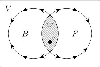
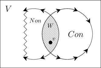
Figure 2. Illustration of the difference between the forward-backward algorithm (left) and the lock-step algorithm (right). On the left, we fully compute both backward ($B$) and forward ($F$) reachable sets from the pivot $v$, identifying $W$ as $F\cap B$. On the right, without loss of generality, assume $F$ is fully computed first. It thus becomes converged ($Con$) and the computation of $B$ ($Non$) is stopped before it is fully explored.

2.3. Lock-step Algorithm

To improve the efficiency of the forward-backward algorithm, the lock-step approach [BGS00] uses another important observation: To compute $W$, it is not necessary to fully compute both $F$ and $B$; only the smaller (in terms of diameter) of the two sets needs to be entirely known. With this observation, the computation of $F$ and $B$ can be modified in the following way: Instead of computing $F$ and $B$ one after the other, the computation is interleaved in a step-by-step manner (dovetailing). When one of the sets is fully computed, the computation of the second set is stopped. Let us call the computed set converged and denote it by $\mathit{Con}$, and the unfinished set non-converged and denote it by $\mathit{Non}$. This situation is illustrated in Figure 2 (right).

However, even when $\mathit{Con}$ is fully known, we still need to finish the computation of states in $\mathit{Non}$ that are inside $\mathit{Con}$ to discover the whole component $W$. This is necessary if there are vertices $w$ in $W$ whose forward distance from $v$ (i.e. the length of the path $v\to^{*}w$) is short while their backward distance (the length of the path $w\to^{*}v$) is long, or vice versa. Such vertices are thus only discovered in one of the two reachability procedures and still need to be discovered by the other one to identify the whole component. However, an important observation is that only the vertices already inside $\mathit{Con}$ need to be considered in this phase.

After this, the SCC can be identified and reported just as in the forward-backward algorithm. Finally, the recursion now continues in sets $\mathit{Con}\setminus W$ and $V\setminus\mathit{Con}$. This is due to $\mathit{Non}$ being not fully computed; we cannot guarantee that no SCC overlaps outside of $\mathit{Non}$ ($\mathit{Non}$ is not necessarily SCC-closed).

The algorithm is still correct because every vertex is eventually either picked as a pivot or discovered in some $W$. Furthermore, due to the way $\mathit{Con}$ and $\mathit{Non}$ are computed guarantees that $W$ is still a whole SCC. In terms of complexity, the algorithm performs $O(|V|\cdot\log|V|)$ symbolic steps in the worst case. To see why this is true, we may observe that every vertex appears in $W$ exactly once, and that the smaller of the two sets $\mathit{Con}\setminus W$ and $V\setminus\mathit{Con}$, let us call it $S$, is always smaller than $\frac{|V|}{2}$. The authors then argue that the price of every iteration can be attributed (up to a multiplicative constant) to the vertices in $S\cup W$ and that every vertex appears in $S$ at most $O(\log|V|)$-times.

2.4. Coloured Lock-step Algorithm

When developing an algorithm for coloured graphs, one needs to deal with multiple challenges which do not appear for monochromatic graphs and require careful consideration. In the following, we refer to the pseudocode in Algorithm 1.

1 Function ColouredSCC$(\mathfrak{G}=(V,C,E))$

2       $\mathfrak{R}_{\mathit{scc}}\subseteq(V\times C\times V)\leftarrow\emptyset$;

3       $\textsc{Decomposition}(\mathfrak{G},\mathfrak{R}_{\mathit{scc}},V\times C)$;

4       return $\mathfrak{R}_{\mathit{scc}}$;

5      

6

7Function Decomposition$(\mathfrak{G}=(V,C,E),\mathfrak{R}_{\mathit{scc}}\subseteq(V\times C\times V),\mathcal{V}\subseteq(V\times C))$

8       if $\mathcal{V}=\emptyset$ then return ;

9       $\mathcal{F},\mathcal{B},\mathcal{F}_{\mathit{open}},\mathcal{B}_{\mathit{open}}\subseteq(V\times C)\leftarrow\textsc{Pivots}(\mathcal{V})$;

10       $\mathcal{F}_{\mathit{paused}},\mathcal{B}_{\mathit{paused}}\subseteq(V\times C)\leftarrow\emptyset$;

11       $F_{\mathit{lock}},B_{\mathit{lock}}\subseteq C\leftarrow\emptyset$;

12       while $F_{\mathit{lock}}\cup B_{\mathit{lock}}\subset\textsc{Colours}(\mathcal{V})$ do

13             $\mathcal{F}_{\mathit{open}}\leftarrow(\textsc{Post}(\mathfrak{G},\mathcal{F}_{\mathit{open}})\cap\mathcal{V})\setminus\mathcal{F}$;

14             $\mathcal{B}_{\mathit{open}}\leftarrow(\textsc{Pre}(\mathfrak{G},\mathcal{B}_{\mathit{open}})\cap\mathcal{V})\setminus\mathcal{B}$;

15             $F_{\mathit{lock}}\leftarrow F_{\mathit{lock}}\cup(\textsc{Colours}(\mathcal{V})\setminus\textsc{Colours}(\mathcal{F}_{\mathit{open}})\setminus B_{\mathit{lock}})$;

16             $B_{\mathit{lock}}\leftarrow B_{\mathit{lock}}\cup(\textsc{Colours}(\mathcal{V})\setminus\textsc{Colours}(\mathcal{B}_{\mathit{open}})\setminus F_{\mathit{lock}})$;

17             $\mathcal{F}_{\mathit{paused}}\leftarrow\mathcal{F}_{\mathit{paused}}\cup(\mathcal{F}_{\mathit{open}}\cap(V\times B_{\mathit{lock}}))$;

18             $\mathcal{B}_{\mathit{paused}}\leftarrow\mathcal{B}_{\mathit{paused}}\cup(\mathcal{B}_{\mathit{open}}\cap(V\times F_{\mathit{lock}}))$;

19             $\mathcal{F}_{\mathit{open}}\leftarrow\mathcal{F}_{\mathit{open}}\setminus(V\times B_{\mathit{lock}})$;

20             $\mathcal{B}_{\mathit{open}}\leftarrow\mathcal{B}_{\mathit{open}}\setminus(V\times F_{\mathit{lock}})$;

21             $\mathcal{F}\leftarrow\mathcal{F}\cup\mathcal{F}_{\mathit{open}}$;

22             $\mathcal{B}\leftarrow\mathcal{B}\cup\mathcal{B}_{\mathit{open}}$;

23            

24       end while

25       $\mathcal{C}on\subseteq V\times C\leftarrow(\mathcal{F}\cap(V\times F_{\mathit{lock}}))\cup(\mathcal{B}\cap(V\times B_{\mathit{lock}}))$;

26       $\mathcal{F}_{\mathit{open}}\leftarrow\mathcal{F}_{\mathit{paused}}\cap\mathcal{C}on$;

27       $\mathcal{B}_{\mathit{open}}\leftarrow\mathcal{B}_{\mathit{paused}}\cap\mathcal{C}on$;

28       while $\mathcal{F}_{\mathit{open}}\neq\emptyset\lor\mathcal{B}_{\mathit{open}}\neq\emptyset$ do

29             $\mathcal{F}_{\mathit{open}}\leftarrow(\textsc{Post}(\mathfrak{G},\mathcal{F}_{\mathit{open}})\cap\mathcal{C}on)\setminus\mathcal{F}$;

30             $\mathcal{B}_{\mathit{open}}\leftarrow(\textsc{Pre}(\mathfrak{G},\mathcal{B}_{\mathit{open}})\cap\mathcal{C}on)\setminus\mathcal{B}$;

31             $\mathcal{F}\leftarrow\mathcal{F}\cup\mathcal{F}_{\mathit{open}}$;

32             $\mathcal{B}\leftarrow\mathcal{B}\cup\mathcal{B}_{\mathit{open}}$;

33            

34       end while

35       $\mathcal{W}\subseteq V\times C\leftarrow\mathcal{F}\cap\mathcal{B}$;

36       $\mathfrak{R}_{\mathit{scc}}\leftarrow\mathfrak{R}_{\mathit{scc}}\cup\textsc{Join}(\mathcal{W})$;

37       $\textsc{Decomposition}(\mathfrak{G},\mathfrak{R}_{\mathit{scc}},\mathcal{V}\setminus\mathcal{C}on)$;

38       $\textsc{Decomposition}(\mathfrak{G},\mathfrak{R}_{\mathit{scc}},\mathcal{C}on\setminus\mathcal{W})$;

39      

40

41Function Pivots$(\mathcal{V})$

42       $\mathcal{P}\subseteq(V\times C)\leftarrow\emptyset$; $\mathcal{V}^{\prime}\subseteq(V\times C)\leftarrow\mathcal{V}$;

43       while $\mathcal{V}^{\prime}\neq\emptyset$ do

44             $(v,c)\leftarrow\textsc{Pick}(\mathcal{V}^{\prime})$;

45             $\mathcal{P}\leftarrow\mathcal{P}\cup(\{v\}\times\sigma_{1}(v,\mathcal{V^{\prime}}))$;

46             $\mathcal{V^{\prime}}\leftarrow\mathcal{V^{\prime}}\setminus(V\times\textsc{Colours}(\mathcal{P}))$;

47            

48       end while

49      return $\mathcal{P}$;

50      

51

Algorithm 1 Symbolic Coloured SCC Decomposition

An important observation is that the structure of components in the graph can change arbitrarily with respect to the graph colours. In consequence, our algorithm cannot simply operate with sets of graph vertices as the normal algorithm would. To that end, we use the notion of coloured vertex sets as introduced in Section 2.1 where the symbolic operations we perform on these sets have been described.

Pivot selection

Initially, the algorithm starts with all vertices and colours, i.e. the full set $V\times C$. However, as the components are discovered, the intermediate results $\mathcal{V}$ may contain different vertices appearing only for certain subsets of $C$. As a result, we often cannot pick a single pivot vertex that would be valid for all considered colours. Instead, we aim to pick a pivot set $P\subseteq V\times C$ such that for every colour that still appears in $\mathcal{V}$, the set contains exactly one vertex. Alternatively, one can also view the pivot set as a (partial) function from $C$ to $V$. This is done in the Pivots function. In the following discussion of the algorithm, we write $c$-coloured pivot to mean the vertex $u$ such that $(u,c)$ is found in the coloured set returned by Pivots in the current iteration (for all colours still present in $\mathcal{V}$).

Please note that the presented Pivots routine is rather naive, as it has to explicitly iterate all the pivot vertices, whose number can be substantial in the worst case. However, as presented, it should be easy to implement for basically any type of coloured graphs, regardless of the underlying representation. In the implementation section, we show Pivots can be re-implemented in the domain of BDDs such that it is guaranteed to always require only $\mathcal{O}(\log|V|)$ symbolic operations.

Coloured lock-step (phase one)

The lock-step reachability procedure also cannot operate as in a standard graph. First of all, there can be colours where the forward reachability converges first, as well as colours where this happens for backward reachability. The algorithm thus has to account for both options simultaneously. Second, for each colour, the reachability can converge in a different number of steps. To deal with this problem, we introduce the $F_{\mathit{lock}}$ and $B_{\mathit{lock}}$ variables. These store the mutually disjoint sets of colours for which the forward and backward reachability procedures have already converged. The lock-step procedure then terminates when $F_{\mathit{lock}}$ and $B_{\mathit{lock}}$ contain all the colours that appear in $\mathcal{V}$.

Throughout the algorithm, we keep track of several coloured-set variables. The first two, $\mathcal{F}$ and $\mathcal{B}$, represent the forward and backward reachable sets, respectively. This means that for every colour $c$ present in $\mathcal{V}$, if $u$ is the $c$-coloured pivot, every $(v,c)\in\mathcal{F}$ satisfies $u\mathrel{\xrightarrow{c}\negthickspace{}^{*}}v$ and every $(v,c)\in\mathcal{B}$ satisfies $v\mathrel{\xrightarrow{c}\negthickspace{}^{*}}u$. Furthermore, if $c\in F_{\mathit{lock}}$ then $\mathcal{F}$ contains exactly all such pairs; similarly for $B_{\mathit{lock}}$ and $\mathcal{B}$.

We say that a coloured vertex pair $(v,c)$ has been forward expanded or backward expanded in the current iteration of the algorithm, if there has been a call to the Post or Pre symbolic operation with $(v,c)$ being an element of the coloured set argument. To track which reachable coloured vertices are to be expanded later, also called the frontiers of the reachability sets, we have the four variables $\mathcal{F}_{\mathit{open}}$, $\mathcal{F}_{\mathit{paused}}$, $\mathcal{B}_{\mathit{open}}$, $\mathcal{B}_{\mathit{paused}}$.

The frontier of $\mathcal{F}$ is the union $\mathcal{F}_{\mathit{open}}\cup\mathcal{F}_{\mathit{paused}}$. The sets $\mathcal{F}_{\mathit{open}}$ and $\mathcal{F}_{\mathit{paused}}$ are disjoint: $\mathcal{F}_{\mathit{open}}$ involves those colours for which the lock-step reachability procedure has not finished yet, i.e. the colours that are neither in $F_{\mathit{lock}}$ nor in $B_{\mathit{lock}}$, while $\mathcal{F}_{\mathit{paused}}$ represents the part of the frontier whose exploration is currently paused due to the fact that its colours are in $B_{\mathit{lock}}$. Note that there may be no pair $(v,c)$ of the forward frontier with $c\in F_{\mathit{lock}}$ as that means that the exploration of the $c$-coloured forward-reachable set is complete. A symmetric role is played by the sets $\mathcal{B}_{\mathit{open}}$ and $\mathcal{B}_{\mathit{paused}}$.

In the first while loop (lines 1–1), we compute the reachability sets in the lock-step manner. Once a reachability set is completed for some colours (i.e., there are no vertices to expand with those colours), we add the colours to the corresponding $F_{\mathit{lock}}$ or $B_{\mathit{lock}}$ variable. Note that we ensure that $F_{\mathit{lock}}$ and $B_{\mathit{lock}}$ remain disjoint even if the two reachability procedures converged at the same time for certain colours—see line 1. We use $F_{\mathit{lock}}$ and $B_{\mathit{lock}}$ to split the newly computed frontier sets into the parts that are to be expanded in the next iteration ($\mathcal{F}_{\mathit{open}}$, $\mathcal{B}_{\mathit{open}}$) and the parts currently left unexpanded ($\mathcal{F}_{\mathit{paused}}$, $\mathcal{B}_{\mathit{paused}}$).

Note that during the computation of Post and Pre on lines 1 and 1, we intersect the resulting set with $\mathcal{V}$. This step is not necessary for correctness, but as the algorithm divides $V\times C$ into smaller sets in each recursive call to Decomposition, it can happen that the set of states reachable from $\mathcal{V}$ is substantially larger than $\mathcal{V}$ itself. In such cases, this intersection effectively restricts the computation of Post and Pre to the sub-graph of $\mathfrak{G}$ induced by $\mathcal{V}$.

Component identification (phase two)

After the first while loop terminates, we compute the set $\mathcal{C}on$ that is an analogue for the converged set of the original lock-step algorithm (line 1). As already suggested above and unlike the original algorithm, this set cannot be just $\mathcal{F}$ or $\mathcal{B}$, but is instead a mixture of both, depending on the converged colours. To compute this set, we use the $F_{\mathit{lock}}$ and $B_{\mathit{lock}}$ variables.

Once $\mathcal{C}on$ is computed, $\mathcal{F}_{\mathit{open}}$ and $\mathcal{B}_{\mathit{open}}$ are restarted using the converged portion of $\mathcal{F}_{\mathit{paused}}$ and $\mathcal{B}_{\mathit{paused}}$ (lines 1 and 1). The second while loop (lines 1–1) can then complete the unfinished forward and backward reachability set, now restricted to the inside of the converged set. The intersection of $\mathcal{F}$ and $\mathcal{B}$ then forms a coloured set $\mathcal{W}$ with the property that for all $c\in\textsc{Colours}(\mathcal{V})$, $\mathcal{W}(\_,c)$ is a strongly connected component of $\mathfrak{G}(c)$. We create the corresponding relation using the Join operation, add this relation to the resulting $\mathfrak{R}_{\mathit{scc}}$, and recursively call the whole procedure with $\mathcal{V}\setminus\mathcal{C}on$ and $\mathcal{C}on\setminus\mathcal{W}$ as the base sets.

Comments on the coloured approach

Let us note that there is possibly another approach to processing coloured graphs. Instead of trying to work with all colours still appearing in the coloured vertex set at once, we could fork a new recursive procedure whenever the colour set splits due to the differences in the graph structure. For example, instead of picking multiple coloured vertices as pivots, one could pick a single vertex with a valid subset of colours and then address the remaining colours in a separate recursive call. Similarly, instead of a single recursive Decomposition call with $\mathcal{C}on\setminus\mathcal{W}$, we could consider two calls, one with the $\mathcal{F}$ portion of $\mathcal{C}on$ and the other with the $\mathcal{B}$ portion of $\mathcal{C}on$ (note that these are colour-disjoint since each colour can converge only in one of the two sets).

While such an approach could be to some extent beneficial in a massively parallel environment where each recursive call can be executed independently on a new CPU, the amount of forking in large systems will soon become unreasonable. More importantly, it defeats the purpose of the symbolic representation, which aims to minimise the number of symbolic operations.

Figure 3. An illustration of the algorithm execution. There are two colours: ${\color[rgb]{1,0,0}\mathit{red}}$ and ${\color[rgb]{0,0,1}\mathit{blue}}$. The left column represents the forward reachability part; the right column represents the backward reachability part. Filled nodes are contained in $\mathcal{F}$, $\mathcal{B}$ respectively. Nodes with solid coloured border are in $\mathcal{F}_{\mathit{open}}$, $\mathcal{B}_{\mathit{open}}$; nodes with dashed coloured border are in $\mathcal{F}_{\mathit{paused}}$, $\mathcal{B}_{\mathit{paused}}$. The bottom-most picture represents the resulting coloured set $\mathcal{W}$.

Example

The execution of one iteration of the algorithm is illustrated in Figure 3. Here, we have an edge-coloured graph with six vertices and two colours (red and blue). The top-most picture represents the initial situation after we have chosen the pivots; in this case, $\{(b,\mathit{blue}),(b,\mathit{red})\}$. The next four rows illustrate the first phase (the first while loop) of the algorithm. After the second iteration of the loop, the blue colour becomes locked in $F_{\mathit{lock}}$, and thus $(f,\mathit{blue})$ is not expanded in the backward reachability procedure. This is illustrated by its dashed outline. After the third iteration of the loop, the red colour becomes locked in $B_{\mathit{lock}}$ and thus the first phase ends. In the second phase, both reachability procedures continue from the paused coloured vertices (dashed outlines); the result is seen in the fifth row. The intersection of the two reachable sets (i.e. the coloured set $\mathcal{W}$) is then illustrated in the bottom-most picture. The algorithm would now continue with the coloured sets $\mathcal{V}\setminus\mathcal{C}on=\{(a,\mathit{blue}),(d,\mathit{blue})\}$ and $\mathcal{C}on\setminus\mathcal{W}=\{(c,\mathit{red})\}$.

2.5. Correctness and Complexity of the Coloured Lock-step Algorithm

Theorem 1.

Let $\mathfrak{G}=(V,C,E)$ be a coloured graph. The coloured lock-step algorithm terminates and computes the coloured SCC decomposition relation $\mathfrak{R}_{\mathit{scc}}$.

Proof 2.1.

We first show that the set $\mathcal{W}$ computed in line 1 indeed contains one SCC for every colour $c\in\textsc{Colours}(\mathcal{V})$ and that the recursive calls of Decomposition preserve the property that $\mathcal{V}$ is SCC-closed with respect to all colours.

Let us assume that $\mathcal{V}$ is SCC-closed and let us take an arbitrary $c\in\textsc{Colours}(\mathcal{V})$. The function Pivots chooses a set that contains exactly one pair whose colour is $c$, let us call this pair $(v,c)$. Let us further assume that $c$ is assigned into $F_{\mathit{lock}}$ first (the case with $B_{\mathit{lock}}$ is completely symmetric).

Let us now choose an arbitrary vertex $w$ such that $v$ and $w$ are in the same SCC of $\mathfrak{G}(c)$, i.e. $v\to^{*}w$ and $w\to^{*}v$. As the first while loop finishes, $\mathcal{F}$ contains all the pairs of the form $(u,c)\in\mathcal{V}$ where $u$ is reachable from $v$ in $\mathfrak{G}(c)$. Thus, it also contains $(w,c)$ due to the fact that $\mathcal{V}$ is SCC-closed. Now, either $(w,c)\in\mathcal{B}$, or there exists a vertex $x$ such that $w\to^{*}x$, $x\to^{*}v$ in $\mathfrak{G}(c)$ and $x\in\mathcal{B}_{\mathit{paused}}$. This means that $(w,c)$ is added to $\mathcal{B}$ in the second while loop. In both cases, both $(v,c)$ and $(w,c)$ are then added to $\mathcal{W}$. As the vertex choices were arbitrary, this proves that the SCC of $v$ in $\mathfrak{G}(c)$ is contained in $\mathcal{W}$. Furthermore, if $(y,c)\in\mathcal{W}$ for an arbitrary $y$, then $v\to^{*}y$ and $y\to^{*}v$ in $\mathfrak{G}(c)$, which means that $y$ is in $SCC(\mathfrak{G}(c),v)$. This proves that $\mathcal{W}$ contains exactly one SCC for every colour $c\in\textsc{Colours}(\mathcal{V})$.

We now argue that $\mathcal{C}on$ is SCC-closed with respect to all colours. This immediately implies that both $\mathcal{V}\setminus\mathcal{C}on$ and $\mathcal{C}on\setminus\mathcal{W}$ are SCC-closed. Let us assume that there is a colour $c\in\textsc{Colours}(\mathcal{V})$ and two vertices $v$, $w$ in the same SCC of $\mathfrak{G}(c)$ such that $(v,c)\in\mathcal{C}on$, but $(w,c)\not\in\mathcal{C}on$. Let us assume that $c\in F_{\mathit{lock}}$ (as above, the case of $B_{\mathit{lock}}$ is completely symmetrical). Then $(v,c)\in\mathcal{F}$ after the first while loop finishes. This also means that $(w,c)\in\mathcal{F}$ as the forward reachability procedure is completed for $c$ and thus $(w,c)\in\mathcal{C}on$, a contradiction.

What remains is to show that the algorithm terminates and that every SCC is eventually found. Termination is trivially proved by the fact that size of the set $\mathcal{V}$ always decreases in recursive calls: both $\mathcal{W}$ and $\mathcal{C}on$ are non-empty because they contain the initial pivot set as a subset. Clearly, a representant of every SCC of every monochromatisation $\mathfrak{G}(c)$ is eventually chosen as a pivot. Together with the above reasoning, this implies that the algorithm is correct.

Theorem 2.

Let $|V|$ be the number of vertices in the coloured graph and let $|C|$ be the number of colours. The coloured lock-step algorithm performs at most $\mathcal{O}(|C|\cdot|V|\cdot\log|V|)$ symbolic steps.

Proof 2.2.

Let us first note that all the derived operations defined in Figure 1 use only a constant number of the basic symbolic operations. As we are considering asymptotic complexity here, we can view all the operations in Figure 1 as elementary symbolic steps.

We first make the observation that each vertex may be chosen as a part of the pivot set at most $|C|$ times. Clearly, once a vertex is included in the pivot set with a set of colours $C^{\prime}$, then, $\{v\}\times C^{\prime}$ is a subset of first $\mathcal{C}on$, and later $\mathcal{W}$ (due to the monotonicity of the construction of $\mathcal{F}$ and $\mathcal{B}$). Therefore, the elements of $\{v\}\times C^{\prime}$ do not appear in subsequent recursive calls. Since a single vertex-colour pair cannot be returned by Pivots twice, it means that the total cumulative complexity of all the calls to the Pivots routine is bounded by $O(|C|\cdot|V|)$. We can therefore exclude them from the rest of the complexity analysis.

We now consider the complexity of a single call to Decomposition without the subsequent recursive calls. Let us now select one of the colours for which the lock-step reachability procedure (lines 1–1) finished last, i.e., one of the colours that have been added to $F_{\mathit{lock}}$ or $B_{\mathit{lock}}$ in the final iteration of the loop. Let us call this colour $c$. Recall that $\sigma_{2}(c,\mathcal{X})$ is the set of vertices with colour $c$ in a coloured set $\mathcal{X}$.

Let us denote by $W$ the monochromatic SCC discovered for $c$, i.e. $W:=\sigma_{2}(c,\mathcal{W})$, and let $S$ be the smaller of $\sigma_{2}(c,\mathcal{V}\setminus\mathcal{C}on)$ and $\sigma_{2}(c,\mathcal{C}on\setminus\mathcal{W})$. Clearly $S$ contains at most $|V|/2$ vertices. Let $k=|S\cup W|$. We now argue that the number of symbolic steps in a given call (without the recursive calls) is bounded by $\mathcal{O}(k)$. This is because in a lock-step algorithm, the call to Decomposition must explore the discovered SCC itself (i.e. $W$), and the smaller of the forward or backward reachable sets from this SCC (i.e. $S$) – intuitively, its complexity should be thus bounded by the size of these two sets.

Assume w.l.o.g. that $c\in F_{\mathit{lock}}$ (a completely symmetric argument solves the case $c\in B_{\mathit{lock}}$). Then after the first while loop finishes, we have $\sigma_{2}(c,\mathcal{C}on)=\sigma_{2}(c,\mathcal{F})$. If $S$ is $\sigma_{2}(c,\mathcal{C}on\setminus\mathcal{W})$ then $k$ is the size of $\sigma_{2}(c,\mathcal{F})$ (and thus also $\sigma_{2}(c,\mathcal{C}on)$), since $\sigma_{2}(c,\mathcal{F})$ consists of $\sigma_{2}(c,\mathcal{C}on\setminus\mathcal{W})$ (the set $S$) and $\sigma_{2}(c,\mathcal{W})$ (the discovered SCC). Each iteration of the first while loop puts at least one vertex with colour $c$ into $\mathcal{F}$; otherwise $c$ would not have finished in the last iteration. This means that the loop runs for at most $k$ iterations. This also means that the size of $\sigma_{2}(x,\mathcal{X})$ for all colours $x$ and $\mathcal{X}\in\{\mathcal{F},\mathcal{B}\}$ is also bounded by $k$ after the first while loop finishes, which in turn means that the second while loop cannot make more than $O(k)$ steps.

If $S$ is $\sigma_{2}(c,\mathcal{V}\setminus\mathcal{C}on)$ instead, let us define $B:=\sigma_{2}(c,\mathcal{B})$ right after the first while loop has finished. We know that $B\subseteq S\cup W$: if a vertex $v$ was in $B\setminus S$, then it would have to be in $\mathcal{C}on$ (i.e. $(v,c)\in\mathcal{C}on$). Due to our initial assumption of $c\in F_{\mathit{lock}}$ (w.l.o.g), we then also have $(v,c)\in\mathcal{F}$ which dictates $v\in W$. Consequently, we see that any vertex $v\in B$ must be either in $S$ or in $W$, arriving at $B\subseteq S\cup W$. Again, each iteration of the first while loop puts at least one vertex with colour $c$ into $\mathcal{B}$; otherwise $c$ would have been in $B_{\mathit{lock}}$ before it appeared in $F_{\mathit{lock}}$. Similarly to the previous case, this means that both while loops run for at most $O(k)$ steps.

The rest of the argument uses amortised reasoning, in a way similar to the proof in [BGS00]. Note that each vertex is going to be an element of the set $W$ as described above at most $|C|$ times (once for each colour). Furthermore, each vertex is going to be an element of the set $S$ as described above at most $|C|\cdot\log|V|$ times: for each colour, the vertex can be an element of the smaller of the two sets at most $\log|V|$ times. As the cost of each single call can be charged to the vertices in $S\cup W$ as explained above, it is sufficient to charge each vertex the total cost of $|C|+|C|\cdot\log|V|$. Together, this means that the total number of symbolic steps is bounded by $O(|C|\cdot|V|\cdot\log|V|)$.

Note that the upper bound established by Theorem 2 is no better than the one we would get if we split the coloured graph into its monochromatic constituents and processed each separately using the original lock-step algorithm [BGS00]. We remark, however, that the practical complexity of the coloured approach can be much smaller. Indeed, the complexity analysis in the previous proof focused on a single colour, omitting the fact that SCCs for many other colours are found at the same time. In cases where the edges are largely shared among the colours, which is true in many applications, the coloured algorithm has the potential to significantly outperform the parameter-scan approach. The situation is similar to that of the coloured model checking; see the observations made in [BBK⁺12].

3. Symbolic Computation with Boolean Networks

The algorithm as presented in the previous section is completely agnostic to the properties of the underlying system, as long one provides an implementation of all the necessary symbolic operations. However, to empirically test its performance, we need to pick such an implementation, which typically entails analysis of a specific class of systems.

In this paper, we consider Boolean networks [Kau69, RCB05, SKI⁺20, Tho73], specifically asynchronous Boolean networks, which represent a popular discrete modelling framework in systems biology [BČŠ13, GBS⁺15]. Due to incomplete biological knowledge, the dynamics of a Boolean network can by often only partially known. This uncertainty can be then captured using coloured directed graphs. In this section, we introduce Boolean networks and show how they can be translated into coloured graphs suitable for SCC-decomposition.

Asynchronous Boolean networks are especially challenging for symbolic analysis. It is a well-known fact, that using symbolic structures (e.g BDDs) to explore very large state spaces gives good results for synchronous systems, but shows its limits when trying to tackle asynchronicity (see e.g. [CT05]).

3.1. Boolean networks with inputs

A Boolean network (BN), as the name suggests, consists of $n$ Boolean variables $s_{1},\ldots,s_{n}$ which together describe the state of the network. The dynamics of the network can also depend on additional $m$ Boolean inputs $c_{1},\ldots,c_{m}$ (sometimes also called constants, or logical parameters), whose value is assumed to be fixed, but generally unknown. The valuations of these inputs correspond to the colours of our Kripke structure.

Each network variable $s_{i}$ is equipped with a Boolean update function $b_{i}:\{0,1\}^{n}\times\{0,1\}^{m}\to\{0,1\}$ that updates the variable based on the state of the network, and the values of its inputs. We assume that the variables are updated asynchronously, meaning that during every state transition, exactly one variable is updated.

Such a network with inputs defines a coloured graph where $V=\{0,1\}^{n}$, $C=\{0,1\}^{m}$, and for every $c\in C$, we have that $u\xrightarrow{c}v$ if and only if $u\not=v$ and $v=u[u_{i}\mapsto b_{i}(u,c)]$ for some $i\in[1,n]$. That is, $v$ is equal to $u$ where the $i$-th variable is updated with the output of function $b_{i}$. Because all variables and inputs are Boolean, this structure has a fairly straightforward symbolic representation in terms of binary decision diagrams, as we later demonstrate.

Note that in practice, we often work within a subset of biologically relevant colours, denoted as $Valid$ (i.e. not every possible valuation of $c_{1},\ldots,c_{m}$ may be biologically admissible). In the algorithms, this is implicitly reflected such that the set of all possible colours $C$ corresponds to the set $Valid$ instead of the set of all possible valuation (i.e. $\{0,1\}^{m}$) if demanded by the application at hand.

3.2. Partially specified Boolean networks

A Boolean network with inputs allows us to easily encode a wide range of biochemical systems in a machine friendly format. However, for systems with a high degree of uncertainty, it often fails to capture this uncertainty in a way understandable to a human reader.

To mitigate this issue, we consider partially specified Boolean networks that allow us to explicitly mark parts of the update functions as unknown. Specifically, let us assume that $f_{1}^{(a_{1})}$, $f_{2}^{(a_{2})}$, $\ldots$ are symbols standing in for some uninterpreted (fixed but arbitrary) Boolean functions (here, $a_{i}$ denotes their arity). A partially specified Boolean network then consists of $n$ Boolean variables and $p$ uninterpreted Boolean functions. In such a network, every update function $b^{\prime}_{i}$ is specified as a Boolean expression that can use the function symbols $f_{1},\ldots,f_{p}$.

This type of formalism is often easier to comprehend, as the uncertainty in dynamics is tied to the update functions instead of inputs (if desired, input can be still expressed using uninterpreted functions of arity zero). It is not immediately clear how such a network should be represented symbolically though.

One option is to translate a partially specified network into a BN with inputs. Any uninterpreted function $f_{i}^{(a)}$ can be encoded in terms of $2^{a}$ Boolean inputs $c_{1}^{i},\ldots,c_{2^{a}}^{i}$ if we consider that input $r_{j}^{i}$ denotes the output of $f_{i}^{(a)}$ in the $j$-th row of its truth table. Formally, this translation can be achieved using a repeated application of the following expansion rule:

$$f(\alpha_{1},\ldots,\alpha_{a})\equiv(\alpha_{1}\Rightarrow f^{\prime}_{1}(\alpha_{2},\ldots,\alpha_{a}))\land(\neg\alpha_{1}\Rightarrow f^{\prime}_{2}(\alpha_{2},\ldots,\alpha_{a}))$$

Here, $f^{\prime}_{1}$ and $f^{\prime}_{2}$ are fresh uninterpreted functions of arity $a-1$, and $\alpha_{i}$ are arbitrary Boolean expressions. Using this rule, we can always convert a partially specified network to a Boolean network with inputs. The number of inputs will be exponential with respect to the arity of the employed uninterpreted functions though (since each application of the rule replaces one uninterpreted function with two, and the depth of the recursive expansion is the arity $a$).

For example, consider the following partially specified Boolean network:

$$b^{\prime}_{1} :=x_{1}\land f_{1}^{(1)}(x_{2})$$

$$b^{\prime}_{2} :=\neg x_{1}\lor f_{2}^{(2)}(x_{1},x_{3})$$

$$b^{\prime}_{3} :=(f_{3}^{(0)}\Leftrightarrow x_{3})\land f_{2}^{(2)}(\neg x_{1},x_{2})$$

It uses three uninterpreted Boolean functions $f_{1}^{(1)}$, $f_{2}^{(2)}$, and $f_{3}^{(0)}$. After performing the aforementioned expansion, and simplifying the resulting expressions slightly for readability, we obtain the following network with logical inputs:

$$b_{1}(x,c)= ~{}x_{1}\land(x_{2}\Rightarrow c^{1}_{[1]})\land(\neg x_{2}\Rightarrow c^{1}_{[0]})$$

$$b_{2}(x,c)= ~{}\neg x_{2}\lor(((x_{1}\land x_{3})\Rightarrow c^{2}_{[1,1]})\land((x_{1}\land\neg x_{3})\Rightarrow c^{2}_{[1,0]})$$

$$\hskip 15.5pt\land~{}((\neg x_{1}\land x_{3})\Rightarrow c^{2}_{[0,1]})\land((\neg x_{1}\land\neg x_{3})\Rightarrow c^{2}_{[0,0]}))$$

$$b_{3}(x,c)= ~{}(c^{3}\Leftrightarrow x_{3})\land((\neg x_{1}\land x_{2})\Rightarrow c^{2}_{[1,1]})\land((\neg x_{1}\land\neg x_{2})\Rightarrow c^{2}_{[1,0]})$$

$$\hskip 57.0pt\land((x_{1}\land x_{2})\Rightarrow c^{2}_{[0,1]})\land((x_{1}\land\neg x_{2})\Rightarrow c^{2}_{[0,0]})$$

Here, each $c^{i}_{j}$ corresponds to one truth table row of $f_{i}$, such that $j$ describes the input vector corresponding to said row (i.e. $c^{1}_{[0,1]}$ represents the value of $f_{1}(0,1)$).

3.3. Symbolic Representation of BNs

As a symbolic representation, a natural choice are Reduced Ordered Binary Decision Diagrams (ROBDD, or simply BDD) [Bry86], which can concisely encode Boolean functions or relations of Boolean vectors. Specifically, out implementation leverages the internal tools and libraries provided by the tool AEON [BBPŠ20].

Since a Boolean network consists of $n$ Boolean variables and $m$ Boolean inputs, any subset of $V$, $C$, or a relation $X\subseteq V\times C$ (a coloured set of vertices) can be seen as a Boolean formula over the network variables and inputs. That is, each network variable and logical input corresponds to one decision variable of the BDD. Here, a pair $(s,c)$ belongs to such a relation iff it represents a satisfying assignment of this formula $X$. For relations of higher arity, fresh decision variables are created for each component of the relation. Standard set operations as described in Fig. 1 then correspond to logical operations on such formulae ($\land\equiv\cap$, $\lor\equiv\cup$, etc.).

Relation operations are similarly implementable using BDD primitives. In particular, existential quantification of a single decision variable (e.g. $\exists s_{i}.X$ or $\exists c_{j}.X$) is a native operation on BDDs. Consequently, existential quantification on relations (as well as Colours) is simply a quantification over all decision variables encoding the specific relation component (i.e. all network variables for $V$, or all logical inputs for $C$). Finally, Swap only influences the way in which a BDD is interpreted – the actual structure of the BDD is unaffected.

To encode the network dynamics, notice that every update function $b_{i}$ can be directly represented as a separate BDD. From such BDDs, we can build one large BDD describing the whole coloured transition relation, which is traditionally used for the computation of Pre and Post. But the symbolic representation of such relation is often prohibitively complex for asynchronous systems. Instead, we compute Pre and Post using partial results for individual variables, which uses more symbolic operations but is less likely to cause a blow-up in the size of the BDD:

$$\textsc{VarPost}(\mathfrak{G},i,\mathcal{X}) =(\mathcal{X}\land(b_{i}\centernot\Leftrightarrow s_{i}))[s_{i}\mapsto\neg s_{i}]$$

$$\textsc{VarPre}(\mathfrak{G},i,\mathcal{X}) =\mathcal{X}[s_{i}\mapsto\neg s_{i}]\land(b_{i}\centernot\Leftrightarrow s_{i})$$

$$\textsc{Post}(\mathfrak{G},\mathcal{X}) =\bigvee_{i\in[1,n]}\textsc{VarPost}(i,\mathcal{X})$$

$$\textsc{Pre}(\mathfrak{G},\mathcal{X}) =\bigvee_{i\in[1,n]}\textsc{VarPre}(i,\mathcal{X})$$

Here, $[s_{i}\mapsto\neg s_{i}]$ is the standard substitution operation, which we use to flip the value of variable $s_{i}$ in the resulting formula if it does not agree with the output of $b_{i}$. Note that this operation can be also implemented structurally directly on the BDD by exchanging the children of decision nodes conditioning on $s_{i}$. Also note that sub-formulae that do not depend on $X$ can be pre-computed once for the whole run of the algorithm, and the version of Pre and Post for monochromatic graphs can be implemented in exactly the same way.

4. Implementation

Finally, let us discuss a number of technical improvements which our algorithm employs in practice, and whose impact we consider in the evaluation section.

4.1. Pivot Selection

In Algorithm 1, we gave a naive implementation of the $\textsc{Pivots}(\mathcal{X})$ function. Here, we show how to implement it for BDDs in a much more concise way. Note that our approach uses the notation we established earlier for Boolean networks, but is generally applicable to any set or relation of bit-vectors represented using BDDs.

First, notice that for a single network variable, we can define a similar operation, which we call $\textsc{Pick}(i,\mathcal{X})$:

$$\textsc{Pick}(i,\mathcal{X})=\mathcal{X}\setminus(\mathcal{X}\land\neg s_{i})[s_{i}\leftarrow\neg s_{i}]$$

Here, we first restrict $\mathcal{X}$ only to the valuations which have $s_{i}=\mathit{false}$, and then invert the value of $s_{i}$ (resulting in $s_{i}$ being always $\mathit{true}$ in the set). Once we subtract these valuations from $\mathcal{X}$, the resulting set then contains a valuation with $s_{i}=\mathit{true}$ only if it does not contain the same valuation with $s_{i}=\mathit{false}$. Intuitively, for any valuation of the remaining BDD decision variables (i.e. $s_{j}$ and $c_{j}$ in our case) that is in $\mathcal{X}$, we just picked a single unique value of $s_{i}$ (while preferring the value $s_{i}=\mathit{false}$).

However, observe that we cannot simply apply Pick to every network variable alone to obtain the result of Pivots. Intuitively, the problem lies in the fact that Pick selects a witness for each variable in isolation, while Pivots considers all network variables as interconnected. We resolve this problem using a different equation, one which eliminates the picked variable in the recursive invocation:

$$\textsc{Pivots}(\mathcal{X}) =\textsc{F}(\mathcal{X},s_{1},\ldots,s_{n})$$

$$\textsc{F}(\mathcal{X},s_{1}) =\textsc{Pick}(1,\mathcal{X})$$

$$\textsc{F}(\mathcal{X},s_{1},\ldots,s_{k}) =\textsc{Pick}(k,\mathcal{X})\cap\textsc{F}(\exists s_{k}.\mathcal{X},s_{1},\ldots,s_{k-1})$$

In this equation, the final case $\textsc{F}(\mathcal{X},s_{1})$ is clearly correct, since it simply defers to $\textsc{Pick}(i,\mathcal{X})$. However, to understand why the recursive case $\textsc{F}(\mathcal{X},s_{1},\ldots,s_{k})$ is correct, observe the following: Assume that the set $\mathcal{Y}=\textsc{F}(\exists s_{k}.\mathcal{X},s_{1},\ldots,s_{k-1})$ is computed correctly. That is, for any valuation of the remaining variables, $\mathcal{Y}$ contains a single unique incomplete witness valuation of variables $s_{1},\ldots,s_{k-1}$. Now, since the BDD representing $\exists s_{k}.\mathcal{X}$ does not depend on $s_{k}$, each such unique witness must be included in $\mathcal{Y}$ twice: once with $s_{k}=\mathit{true}$ and once with $s_{k}=\mathit{false}$. In other words, a single witness valuation of $s_{1},\ldots,s_{k-1}$ must be tied to two different valuations of the remaining variables, and these valuations are differentiated only by the variable $s_{k}$.

Now, one of these two valuations is necessarily included in the set $\textsc{Pick}(k,\mathcal{X})$. The other is either missing from $\mathcal{X}$ altogether, or is eliminated by $\textsc{Pick}(k,\mathcal{X})$. As such, computing $\textsc{Pick}(k,\mathcal{X})\cap\mathcal{Y}$ extends the witness from $s_{1},\ldots,s_{k-1}$ to $s_{1},\ldots,s_{k}$ by eliminating one of the two aforementioned occurrences of the incomplete witness.

Observe that, as opposed to the original naive implementation of Pivots, this implementation only requires $\mathcal{O}(n)$ (i.e. $\mathcal{O}(\log|V|)$) symbolic operations in any case.

4.2. Saturation

In [CMS06], and later in greater detail within [ZC11], Ciardo et al. show that when the system is asynchronous, it may be much easier to compute reachable sets (and consequently SCCs) by applying only one transition (e.g. denoted $t_{1}$) at a time. Once applying $t_{1}$ cannot add new states to the reachable set, another transition (e.g denoted $t_{2}$) can be considered, respecting the order in which the affected variables appear in the symbolic data structure (Ciardo et al. employ multivalued decision diagrams, but the principle also applies to BDDs). If the application of other transitions causes that we can again add new states using $t_{1}$, the process starts anew and $t_{1}$ is “saturated” again.

In the comparison presented in [ZC11], only the Xie-Beerel $\mathcal{O}(|V|^{2})$ algorithm is used with saturation enabled, while the lock-step algorithm is used as given in [BGS00]. However, we argue that saturation can be also beneficial in the lock-step algorithm.

Asymptotic complexity

Unfortunately, combining lock-step with saturation disrupts the $\mathcal{O}(|V|\cdot\log|V|)$ asymptotic complexity of the algorithm. To see why this is the case, observe that classical symbolic reachability (i.e. a fixed-point algorithm iterating the Post procedure) requires $\mathcal{O}(|V|)$ steps to explore a graph. Meanwhile, a reachability procedure employing saturation needs $\mathcal{O}(|V||T|)$ operations, where $|T|$ is the number of distinct transitions.

This is caused by the fact that saturation needs to check up to $|T|$ transitions to discover a vertex. For example, consider an asynchronous graph employing transitions $t_{1},\ldots,t_{n}$ such that $t_{1}$ and $t_{n}$ are alternated on a path of length $\mathcal{O}(|V|)$. Between considering $t_{1}$ and $t_{n}$, saturation will attempt each of the $|T|$ transitions, which are useless on this path, but still consume a symbolic operation.

Consequently, this $|T|$ factor trickles down into the complexity of both the Xie-Beerel and lock-step algorithms if saturation is used, as both ultimately rely on some form of reachability to discover the graph vertices. The complexity of the coloured algorithms is then similarly affected.

Saturation and lock-step

The main idea of how saturation is applied in a coloured lock-step algorithm (for Boolean networks) is shown in Algorithm 2. The algorithm presents a helper function which performs one reachability step, similar to what is performed by the Post function. However, in this algorithm, only one transition is fired for each colour (we assume the iteration follows the order of variables as they appear in the symbolic representation, which benefits saturation). Additionally, a set $R$ of colours that could not perform a step is computed. A similar procedure can be considered for backwards reachability, simply replacing VarPost with VarPre.

Note that there is a slight discrepancy between Algorithm 2 and the intuitive description of saturation that we gave earlier. In particular, we see that during a NextStep operation, a transition for each variable is triggered at most once, as opposed to the original description, where a transitions are fired repeatedly. This is caused by the simple nature of Boolean networks: In a BN, a single transition always modifies a single Boolean variable. Consequently, no new states can be discovered by firing a single transition multiple times in sequence. For other asynchronous systems, VarPost may need to be modify to apply the corresponding transition repeatedly.

Additionally, note that we use the set $R$ to ensure that VarPost (i.e. firing of a single transition) is executed only for colours for which we have not found a successor yet using some of the previously considered transitions. This is necessary to ensure that in each invocation of NextStep, each colour present in $\mathcal{F}$ is either advanced by one step (using exactly one transition), or is reported as converged within the returned set $R$.

Using this process, we can replace the $\textsc{Pre}/\textsc{Post}$ procedures in the main lock-step algorithm (lines 11 and 12 of Algorithm 1). The $R$ sets computed here are then used to update $F_{lock}$ and $B_{lock}$ (lines 13 and 14), as they exactly represent the converged colours that do not need further computation. A similar modification is necessary for the second while loop (lines 25-29), but here the sets of remaining colours $R$ are not needed.

1 Function NextStep$(\mathfrak{G},\mathcal{F})$

2       $R\leftarrow\textsc{Colours}(\mathcal{F})$;

3       for $\mathtt{A}\in\mathit{Var}$ do

4             $\mathcal{S}\leftarrow\textsc{VarPost}(\mathfrak{G},\mathtt{A},(\mathcal{F}\cap V)\times R)$;

5             $R\leftarrow R\setminus\textsc{Colours}(\mathcal{S})$;

6             $\mathcal{F}\leftarrow\mathcal{F}\cup\mathcal{S}$;

7             if $R=\emptyset$ then

8                  break;

9             end if

10            

11       end for

12      return $\mathcal{(}\mathcal{F},R)$;

13      

14

Algorithm 2 Main idea of the lock-step-saturation approach. The algorithm extends $\mathcal{F}$ with one additional reachability step, and returns a set of colours locked in this iteration ($R$).

4.3. Trimming and Parallelism

Most graphs typically contain a large number of trivial SCCs that introduce unnecessary overhead to the main algorithm. To avoid this overhead, we additionally perform a trimming step before each invocation of Decomposition. Trimming consists of repeatedly removing all vertices which have no outgoing or no incoming edges and is employed by most symbolic SCC algorithms on standard directed graphs as well.

The coloured analogue of trimming is straightforward, as it can be achieved using Pre and Post operations just as in the non-coloured case. For a coloured set of vertices $\mathcal{V}$, operation $\textsc{Post}(\mathfrak{G},\textsc{Pre}(\mathfrak{G},\mathcal{V})\cap\mathcal{V})\cap\mathcal{V}$ returns only the vertices which have at least one predecessor in $\mathcal{V}$. The successor variant simply exchanges the Post and Pre operations.

As such, applying this operation to each $\mathcal{V}$ until a fixed-point is reached before Decomposition is invoked eliminates the undesired trivial SCCs. Since the total number of steps performed collectively by all such fixed-point computations is bounded by $|C||V|$ (the total number of removable vertex-colour pairs), this does not impact the overall asymptotic complexity of the algorithm.

In some cases, we have observed that the symbolic representation is able to handle the SCC computation but explodes during trimming. The algorithm then times-out during trimming, even though useful information about SCCs could be obtained if the trimming was skipped or postponed. To avoid this issue, we enforce an extra condition that a trimming procedure is terminated prematurely if the computed BDDs are more than twice the size (in terms of BDD decision nodes) of the initial set.

Additionally, the lock-step algorithm can be rather trivially parallelised. The recursive Decomposition calls operate on independent coloured vertex sets and can be therefore deferred to separate threads. Since the body of the Decomposition method is rather complex, this can be done easily with a queue guarded by a mutex which is shared between all threads (i.e. the synchronisation overhead is negligible due to the long running time of Decomposition). Finally, a simple termination detection procedure is needed to ensure that idle threads do not terminate prematurely while decomposition is still running.

Note that most BDD packages are not internally thread-safe, as they share decision node memory across different BDD objects. In our experiments, this aspect is handled by cloning the set $\mathcal{V}$ corresponding to each recursive invocation, plus the symbolic representation of the BN necessary to compute Post and Pre. As such, the memory used to represent BDDs manipulated by each thread is completely independent from other threads.

5. Experimental Evaluation

To test the algorithm, we compiled a benchmark set of Boolean networks from the CellCollective [HKM⁺12] and GINsim [CNT12] model databases. Since the models in these databases contain fully specified networks, uninterpreted functions were introduced into existing models by pseudo-randomly erasing parts of the existing update functions.

While this process is to some extent artificial, we believe it to be a good approximation of the model development process, where at some point, the structure of the network is already established, but its dynamics are still not fully determined. Using this process, we obtained a collection of networks ranging between $2^{20}$ and $2^{50}$ in the size of the coloured graph (i.e. $|V\times C|$). Note that for each graph, we consider only a subset of possible input valuations that is biologically relevant with respect to the established network structure. For example, the first model (i.e. [SOHMMA17]) admits $2^{48}$ input valuations, but only $2^{19}$ are biologically relevant due to constraints on function monotonicity.

A complete overview of the employed models is given in Table 1. For each model, we give the number of discovered non-trivial components as an interval, because each colour can correspond to a different number of components. We employ a 24h timeout for all experiments.

Table 1. The considered benchmark models. Here, $n$ is the number of BN variables, $m$ is the number of logical inputs (after expansion of uninterpreted functions), $|C|$ is the number of all biologically relevant colours (input valuations), and $|V\times C|$ is the size of the whole biologically relevant coloured state space. Finally, #SCC gives the number of detected non-trivial SCCs. Note that this number varies depending on input valuation, and is thus given as a range.

Model name	$n$	$m$	$|C|$	$|V\times C|$	#SCC
Asymmetric Cell Division [SOHMMA17]	$5$	$48$	$\sim 2^{19}$	$\sim 2^{24}$	1-13
Reduced TCR Signalisation [KSRL+06]	$10$	$46$	$\sim 2^{14}$	$\sim 2^{24}$	36-115
Budding Yeast (Orlando) [OLB+08]	$9$	$54$	$\sim 2^{16}$	$\sim 2^{27}$	1-16
Budding Yeast (Irons) [Iro09]	$18$	$44$	$\sim 2^{17}$	$\sim 2^{35}$	2-5568
Tumor Cell Migration [CMR+15]	$20$	$44$	$\sim 2^{15}$	$\sim 2^{35}$	436-379308
T-cell Differentiation [MX06]	$23$	$40$	$\sim 2^{15}$	$\sim 2^{38}$	41728-43264
WG Signalling Pathway [MJB+13]	$26$	$38$	$\sim 2^{22}$	$\sim 2^{48}$	0
Full TCR Signalisation [KSRL+06]	$30$	$48$	$\sim 2^{17}$	$\sim 2^{47}$	48-1087

Table 2. Overview of runtime for different version of the SCC detection algorithm. The times (hours:minutes:seconds) refer to the total runtime of the SCC decomposition procedure for the basic lock-step, lock-step with saturation, and lock-step with saturation and parallelism, with DNF representing a time-out after 24-hours.

Model Name	Parallel	Satur.	Lock-step
Asymmetric Cell Division [SOHMMA17]	00:05	00:10	00:15
Reduced TCR Signalisation [KSRL+06]	00:04	00:45	01:12
Budding Yeast (Orlando) [OLB+08]	06:29	06:50	11:21
Budding Yeast (Irons) [Iro09]	15:14	2:53:16	3:28:44
Tumor Cell Migration [CMR+15]	40:10	18:34:16	DNF
T-cell Differentiation [MX06]	16:10:41	DNF	DNF
WG Signalling Pathway [MJB+13]	1:18:38	1:23:37	1:42:12
Full TCR Signalisation [KSRL+06]	4:49:04	DNF	DNF

The experiments were performed on a 32-core AMD Threadripper workstation with 64GB of RAM memory. All tested models are available in our source code repository. Note that the smaller models ($<2^{30}$) should be easy to process even on a less powerful machine; however, the larger models can require substantial amount of memory.

For each model, we have tested the lock-step algorithm as presented in the main part of this paper (Lock-step in Table 2), an enhanced version with saturation enabled (Satur. in Table 2), and a parallel implementation which also includes saturation (Parallel in Table 2). In all algorithms, we employ the trimming optimisation.

From the results, we can see that parallelisation improves the performance of the algorithm significantly: in case of models with a large number of SCCs, we see an up-to 30x speed-up, comparing Parallel and Satur. in Table 2. On the other hand, when the number of SCCs is small (such as [OLB⁺08]), the speed-up is understandably minimal, since the number of independent recursive calls is also small.

As expected, the total number of SCCs has a significant impact on the performance of the algorithm (e.g. [Iro09] and [CMR⁺15]) overall, since the number of calls to Decomposition increases. Furthermore, we see that our “coloured saturation” indeed provides a performance benefit. However, this improvement is mostly incremental.

After further analysis, we discovered that the whole algorithm is often limited by the performance of the trimming procedure, rather than reachability procedures though. In particular, the use of saturation has significantly reduced the size of symbolic representation during computation of reachability, however the symbolic representation still performs rather poorly (at least for Boolean networks) during trimming. This limits the performance of the whole method, since all the considered graphs contain a large portion of trivial SCCs. Furthermore, in many cases the number of iterations needed to completely trim a set of states is substantial. This leads us to believe there is still space for improvement in terms of SCC detection in large Boolean networks, even without parameters.

Finally, we examined the benefit of processing all colours simultaneously versus a naive parameter scan approach, where each monochromatic case is handled separately. To do so, we considered various pseudo-random monochromatisations of the studied models and processed these using our algorithm. Here, we observe that for the four models with at least $20$ variables, no computation for any of the monochromatic models finished in under one second (with T-cell differentiation typically requiring more than one minute due to the relatively large number of components).

Consequently, we can extrapolate that computing the full coloured SCC decomposition using such naive parameter scan would require more than 10 ours for each model (and $10+$ days in the case of T-cell differentiation). This approach could be to some extent beneficial in a massively parallel environment (hundreds or thousands of CPUs), but the coloured approach clearly scales better in setups where resources are more limited.

6. Conclusions

This paper presents a fully symbolic algorithm for detecting all monochromatic strongly connected components in edge-coloured graphs. The work has been motivated by systems sciences, namely systems biology, where the need for efficient automated analysis of components in large graphs with a large sets of coloured edges is emerging. The algorithm combines several ideas inspired by existing state-of-the-art algorithms for SCC decomposition in a non-trivial way. We believe this is the first fully symbolic algorithm aiming to solve the problem efficiently.

The experimental evaluation has shown that the algorithm can handle large, real-world systems that would be otherwise too large to fit into the memory of a conventional workstation ($>2^{32}$), and that the performance of the algorithm can be further improved using saturation and parallelisation. Finally, the algorithm has a strong potential to be significantly faster than iterating a standard algorithm for SCC decomposition executed on all monochromatic sub-graphs one-by-one.

References

- [AA07] S. Akbari and A. Alipour. Multicolored trees in complete graphs. Journal of Graph Theory, 54(3):221–232, 2007.
- [ADF+08] A. Abouelaoualim, K. Ch. Das, L. Faria, Y. Manoussakis, C. Martinhon, and R. Saad. Paths and trails in edge-colored graphs. In LATIN 2008: Theoretical Informatics, pages 723–735. Springer, 2008.
- [AG97] N. Alon and G. Gutin. Properly colored hamilton cycles in edge-colored complete graphs. Random Structures & Algorithms, 11(2):179–186, 1997.
- [BBB+17] Jiří Barnat, Nikola Beneš, Luboš Brim, Martin Demko, Matej Hajnal, Samuel Pastva, and David Šafránek. Detecting attractors in biological models with uncertain parameters. In Computational Methods in Systems Biology (CMSB 2017), volume 10545 of Lecture Notes in Computer Science, pages 40–56. Springer, 2017.
- [BBBv11] Jiří Barnat, Petr Bauch, Luboš Brim, and Milan Češka. Computing strongly connected components in parallel on CUDA. In 25th IEEE International Symposium on Parallel and Distributed Processing, IPDPS 2011 - Conference Proceedings, pages 544–555. IEEE, 2011.
- [BBK+12] J. Barnat, L. Brim, A. Krejci, A. Streck, D. Safranek, M. Vejnar, and T. Vejpustek. On parameter synthesis by parallel model checking. IEEE/ACM Transactions on Computational Biology and Bioinformatics, 9(3):693–705, 2012.
- [BBP+19] Nikola Beneš, Luboš Brim, Samuel Pastva, Jakub Poláček, and David Šafránek. Formal analysis of qualitative long-term behaviour in parametrised boolean networks. In Formal Methods and Software Engineering (ICFEM 2019), volume 11852 of Lecture Notes in Computer Science, pages 353–369. Springer, 2019.
- [BBPŠ20] Nikola Beneš, Luboš Brim, Samuel Pastva, and David Šafránek. AEON: attractor bifurcation analysis of parametrised boolean networks. In Computer Aided Verification - 32nd International Conference, CAV 2020, volume 12224 of Lecture Notes in Computer Science, Cham, 2020. Springer International Publishing.
- [BBPŠ21] Nikola Beneš, Luboš Brim, Samuel Pastva, and David Šafránek. Symbolic coloured SCC decomposition. In International Conference on Tools and Algorithms for the Construction and Analysis of Systems, pages 64–83. Springer, 2021.
- [BCLF79] Mehdi Behzad, Gary Chartrand, and Linda Lesniak-Foster. Graphs and Digraphs. Wadsworth Publishing, 1979.
- [BCM+92] Jerry R. Burch, Edmund M. Clarke, Kenneth L. McMillan, David L. Dill, and L. J. Hwang. Symbolic model checking: 10^20 states and beyond. Inf. Comput., 98(2):142–170, 1992.
- [BČŠ13] Luboš Brim, Milan Češka, and David Šafránek. Model checking of biological systems. In Formal Methods for Dynamical Systems, pages 63–112. Springer Berlin Heidelberg, 2013.
- [BCVDP11] Jiří Barnat, Jakub Chaloupka, and Jaco Van De Pol. Distributed algorithms for SCC decomposition. J. Log. and Comput., 21(1):23–44, 2011.
- [BGS00] Roderick Bloem, Harold N. Gabow, and Fabio Somenzi. An algorithm for strongly connected component analysis in n log n symbolic steps. In Formal Methods in Computer-Aided Design (FMCAD 2000), Lecture Notes in Computer Science, pages 37–54. Springer-Verlag, 2000.
- [BJG97] Joergen Bang-Jensen and Gregory Gutin. Alternating cycles and paths in edge-coloured multigraphs: A survey. Discrete Mathematics, 165-166:39 – 60, 1997.
- [BLvdP16] Vincent Bloemen, Alfons Laarman, and Jaco van de Pol. Multi-core on-the-fly SCC decomposition. In Proceedings of the 21st ACM SIGPLAN Symposium on Principles and Practice of Parallel Programming, PPoPP ’16, New York, NY, USA, 2016. ACM.
- [BPC+10] Grégory Batt, Michel Page, Irene Cantone, Gregor Goessler, Pedro T. Monteiro, and Hidde de Jong. Efficient parameter search for qualitative models of regulatory networks using symbolic model checking. Bioinformatics, 26(18), 2010.
- [Bry86] R. E. Bryant. Graph-based algorithms for boolean function manipulation. IEEE Trans. Comput., 35(8):677–691, 1986.
- [CC16] Sang-Mok Choo and Kwang-Hyun Cho. An efficient algorithm for identifying primary phenotype attractors of a large-scale boolean network. BMC Systems Biology, 10(1):95, 2016.
- [CDHL18] Krishnendu Chatterjee, Wolfgang Dvořák, Monika Henzinger, and Veronika Loitzenbauer. Lower bounds for symbolic computation on graphs: Strongly connected components, liveness, safety, and diameter. In Proceedings of the Twenty-Ninth Annual ACM-SIAM Symposium on Discrete Algorithms (SODA 2018), pages 2341–2356. SIAM, 2018.
- [CHS+10] Andreas Classen, Patrick Heymans, Pierre-Yves Schobbens, Axel Legay, and Jean-François Raskin. Model checking lots of systems: efficient verification of temporal properties in software product lines. In Proceedings of the 32nd ACM/IEEE International Conference on Software Engineering-Volume 1, pages 335–344, 2010.
- [CMR+15] David PA Cohen, Loredana Martignetti, Sylvie Robine, Emmanuel Barillot, Andrei Zinovyev, and Laurence Calzone. Mathematical modelling of molecular pathways enabling tumour cell invasion and migration. PLoS computational biology, 11(11):e1004571, 2015.
- [CMS06] Gianfranco Ciardo, Robert M. Marmorstein, and Radu Siminiceanu. The saturation algorithm for symbolic state-space exploration. Int. J. Softw. Tools Technol. Transf., 8(1):4–25, 2006.
- [CNT12] Claudine Chaouiya, Aurelien Naldi, and Denis Thieffry. Logical modelling of gene regulatory networks with ginsim. In Bacterial Molecular Networks, pages 463–479. Springer, 2012.
- [CT05] Jean-Michel Couvreur and Yann Thierry-Mieg. Hierarchical decision diagrams to exploit model structure. In FORTE 2005, volume 3731 of Lecture Notes in Computer Science, pages 443–457. Springer, 2005. doi:10.1007/11562436\_32.
- [DAERR16] Dávid Deritei, William C Aird, Mária Ercsey-Ravasz, and Erzsébet Ravasz Regan. Principles of dynamical modularity in biological regulatory networks. Nature Scientific Reports, 6:21957, 2016.
- [Dor94] Dietmar Dorninger. Hamiltonian circuits determining the order of chromosomes. Discrete Applied Mathematics, 50(2):159 – 168, 1994.
- [FHP00] Lisa K. Fleischer, Bruce Hendrickson, and Ali Pınar. On identifying strongly connected components in parallel. In Parallel and Distributed Processing, volume 1800 of Lecture Notes in Computer Science, pages 505–511. Springer, 2000.
- [GBS+15] Melanie Grieb, Andre Burkovski, J. Eric Sträng, Johann M. Kraus, Alexander Groß, Günther Palm, Michael Kühl, and Hans A. Kestler. Predicting variabilities in cardiac gene expression with a boolean network incorporating uncertainty. PLOS ONE, 10(7):1–15, 07 2015.
- [GGG+17] Mirco Giacobbe, Calin C. Guet, Ashutosh Gupta, Thomas A. Henzinger, Tiago Paixão, and Tatjana Petrov. Model checking the evolution of gene regulatory networks. Acta Informatica, 54(8):765–787, 2017.
- [GPP03] Raffaella Gentilini, Carla Piazza, and Alberto Policriti. Computing strongly connected components in a linear number of symbolic steps. In Proceedings of the Twenty-Ninth Annual ACM-SIAM Symposium on Discrete Algorithms (SODA 2003), volume 3, pages 573–582. SIAM, 2003.
- [GPP08] Raffaella Gentilini, Carla Piazza, and Alberto Policriti. Symbolic graphs: Linear solutions to connectivity related problems. Algorithmica, 50(1):120–158, 2008.
- [HKM+12] Tomáš Helikar, Bryan Kowal, Sean McClenathan, Mitchell Bruckner, Thaine Rowley, Alex Madrahimov, Ben Wicks, Manish Shrestha, Kahani Limbu, and Jim A Rogers. The cell collective: toward an open and collaborative approach to systems biology. BMC systems biology, 6(1):1–14, 2012.
- [HRO13] Sungpack Hong, Nicole C. Rodia, and Kunle Olukotun. On fast parallel detection of strongly connected components (SCC) in small-world graphs. In Proceedings of the International Conference on High Performance Computing, Networking, Storage and Analysis, SC 2013, New York, NY, USA, 2013. ACM.
- [Iro09] DJ Irons. Logical analysis of the budding yeast cell cycle. Journal of theoretical biology, 257(4):543–559, 2009.
- [Jia93] Bin Jiang. I/O- and CPU-optimal recognition of strongly connected components. Information Processing Letters, 45(3):111 – 115, 1993.
- [Kau69] S.A. Kauffman. Metabolic stability and epigenesis in randomly constructed genetic nets. Journal of Theoretical Biology, 22(3):437–467, 1969.
- [Kir14] Zoltán Király. Monochromatic components in edge-colored complete uniform hypergraphs. European Journal of Combinatorics, 35:374 – 376, 2014.
- [KL08] Mikio Kano and Xueliang Li. Monochromatic and heterochromatic subgraphs in edge-colored graphs - a survey. Graphs and Combinatorics, 24(4):237–263, 2008.
- [KSRL+06] Steffen Klamt, Julio Saez-Rodriguez, Jonathan A Lindquist, Luca Simeoni, and Ernst D Gilles. A methodology for the structural and functional analysis of signaling and regulatory networks. BMC bioinformatics, 7(1):56, 2006.
- [LWA+16] Qin Li, Anders Wennborg, Erik Aurell, Erez Dekel, Jie-Zhi Zou, Yuting Xu, Sui Huang, and Ingemar Ernberg. Dynamics inside the cancer cell attractor reveal cell heterogeneity, limits of stability, and escape. Proceedings of the National Academy of Sciences, 113(10):2672–2677, 2016.
- [LZCY14] Guohui Li, Zhe Zhu, Zhang Cong, and Fumin Yang. Efficient decomposition of strongly connected components on GPUs. Journal of Systems Architecture, 60(1):1 – 10, 2014.
- [Mat20] A.E. Matouk. Complex dynamics in susceptible-infected models for covid-19 with multi-drug resistance. Chaos, Solitons & Fractals, 140:110257, 2020.
- [MJB+13] Abibatou Mbodj, Guillaume Junion, Christine Brun, Eileen EM Furlong, and Denis Thieffry. Logical modelling of drosophila signalling pathways. Molecular BioSystems, 9(9):2248–2258, 2013.
- [MPQY19] A. Mizera, J. Pang, H. Qu, and Q. Yuan. Taming asynchrony for attractor detection in large boolean networks. IEEE/ACM Transactions on Computational Biology and Bioinformatics, 16(1):31–42, 2019.
- [MX06] Luis Mendoza and Ioannis Xenarios. A method for the generation of standardized qualitative dynamical systems of regulatory networks. Theoretical Biology and Medical Modelling, 3(1):13, 2006.
- [OLB+08] David A Orlando, Charles Y Lin, Allister Bernard, Jean Y Wang, Joshua ES Socolar, Edwin S Iversen, Alexander J Hartemink, and Steven B Haase. Global control of cell-cycle transcription by coupled CDK and network oscillators. Nature, 453(7197):944–947, 2008.
- [Orz05] Simona Orzan. On Distributed Verification and Verified Distribution. PhD thesis, Free University Amsterdam, 2005.
- [PIS+21] Tatjana Petrov, Claudia Igler, Ali Sezgin, Thomas A Henzinger, and Calin C Guet. Long lived transients in gene regulation. Theoretical Computer Science, 893:1–16, 2021.
- [RCB05] Adrien Richard, Jean-Paul Comet, and Gilles Bernot. Graph-based modeling of biological regulatory networks: Introduction of singular states. In Computational Methods in Systems Biology (CMSB 2005), volume 3082 of Lecture Notes in Computer Science, pages 58–72. Springer, 2005.
- [Rei85] John H. Reif. Depth-first search is inherently sequential. Information Processing Letters, 20(5):229 – 234, 1985.
- [Saa92] R. Saad. Sur quelques problèmes de complexité dans les graphes. PhD thesis, U. de Paris-Sud, Orsay, 1992.
- [Sha81] M. Sharir. A strong-connectivity algorithm and its applications in data flow analysis. Computers & Mathematics with Applications, 7(1):67–72, 1981.
- [SKI+20] Julian D. Schwab, Silke D. Kühlwein, Nensi Ikonomi, Michael Kühl, and Hans A. Kestler. Concepts in boolean network modeling: What do they all mean? Computational and Structural Biotechnology Journal, 18:571–582, 2020.
- [SOHMMA17] Ismael Sánchez-Osorio, Carlos A Hernández-Martínez, and Agustino Martínez-Antonio. Modeling asymmetric cell division in caulobacter crescentus using a boolean logic approach. In Asymmetric Cell Division in Development, Differentiation and Cancer, pages 1–21. Springer, 2017.
- [SRM14] G. M. Slota, S. Rajamanickam, and K. Madduri. BFS and coloring-based parallel algorithms for strongly connected components and related problems. In 2014 IEEE 28th International Parallel and Distributed Processing Symposium, pages 550–559, 2014.
- [SRR+18] Will Steffen, Johan Rockström, Katherine Richardson, Timothy M. Lenton, Carl Folke, Diana Liverman, Colin P. Summerhayes, Anthony D. Barnosky, Sarah E. Cornell, Michel Crucifix, Jonathan F. Donges, Ingo Fetzer, Steven J. Lade, Marten Scheffer, Ricarda Winkelmann, and Hans Joachim Schellnhuber. Trajectories of the earth system in the anthropocene. Proceedings of the National Academy of Sciences, 115(33):8252–8259, 2018.
- [Tar72] Robert Endre Tarjan. Depth-first search and linear graph algorithms. SIAM J. Comput., 1(2):146–160, 1972.
- [Tho73] René Thomas. Boolean formalization of genetic control circuits. Journal of Theoretical Biology, 42(3):563–585, 1973.
- [TW07] Andrew Thomason and Peter Wagner. Complete graphs with no rainbow path. Journal of Graph Theory, 54(3):261–266, 2007.
- [WKB14] Anton Wijs, Joost-Pieter Katoen, and Dragan Bošnački. GPU-based graph decomposition into strongly connected and maximal end components. In Computer Aided Verification (CAV 2014), volume 8559 of Lecture Notes in Computer Science, pages 310–326. Springer, 2014.
- [XB00] Aiguo Xie and Peter A Beerel. Implicit enumeration of strongly connected components and an application to formal verification. IEEE Transactions on Computer-Aided Design of Integrated Circuits and Systems, 19(10):1225–1230, 2000.
- [YMPQ19] Qixia Yuan, Andrzej Mizera, Jun Pang, and Hongyang Qu. A new decomposition-based method for detecting attractors in synchronous boolean networks. Science of Computer Programming, 180:18–35, 2019.
- [ZC11] Yang Zhao and Gianfranco Ciardo. Symbolic computation of strongly connected components and fair cycles using saturation. Innov. Syst. Softw. Eng., 7(2):141–150, 2011.
- [ZHA+07] Shu-Qin Zhang, Morihiro Hayashida, Tatsuya Akutsu, Wai-Ki Ching, and Michael K. Ng. Algorithms for finding small attractors in Boolean networks. EURASIP J. Bioinformatics Syst. Biol., 2007:4–4, January 2007.