A wide-field CO survey towards the California Molecular Filament

Abstract

We present the survey of ¹²CO/¹³CO/C¹⁸O (J=1-0) toward the California Molecular Cloud (CMC) within the region of 161.75$\arcdeg\leqslant l\leqslant$ 167.75$\arcdeg$, -9.5$\arcdeg\leqslant b\leqslant$ -7.5$\arcdeg$, using the Purple Mountain Observatory (PMO) 13.7 m millimeter telescope. Adopting a distance of 470 pc, the mass of the observed molecular cloud estimated from ¹²CO, ¹³CO, and C¹⁸O is about 2.59$\times$10⁴ M_⊙, 0.85$\times$10⁴ M_⊙, and 0.09$\times$10⁴ M_⊙, respectively. A large-scale continuous filament extending about 72 pc is revealed from the ¹³CO images. A systematic velocity gradient perpendicular to the major axis appears and is measured to be $\sim$ 0.82 km s^-1 pc^-1. The kinematics along the filament shows an oscillation pattern with a fragmentation wavelength of $\sim$ 2.3 pc and velocity amplitude of $\sim 0.92\mathrm{~{}km}\mathrm{~{}s}^{-1}$, which may be related with core-forming flows. Furthermore, assuming an inclination angle to the plane of the sky of $45^{\circ}$, the estimated average accretion rate is $\sim$ 101 M_⊙ Myr^-1 for the cluster LkH$\alpha$ 101 and $\sim$ 21 M_⊙ Myr^-1 for the other regions. In the C¹⁸O observations, the large-scale filament could be resolved into multiple substructures and their dynamics are consistent with the scenario of filament formation from converging flows. Approximately 225 C¹⁸O cores are extracted, of which 181 are starless cores. Roughly $37\,\%\,(67/181)$ of the starless cores have $\alpha_{\text{vir}}$ less than 1. Twenty outflow candidates are identified along the filament. Our results indicate active early-phase star formation along the large-scale filament in the CMC region.

1 Introduction

Filamentary structures are ubiquitous in the interstellar medium (ISM). In the last decade, based on multi-wavelength observations (e.g., surveys with the $Herschel$ Space Observatory), great progresses have been made in the relationship between filamentary molecular clouds and star formation (André et al., 2010; Molinari et al., 2010). It is widely accepted that filamentary molecular clouds play an important role in the process of star formation. Both observational and theoretical studies suggest that large-scale supersonic compressed gas forms reticular structures firstly in the ISM, and then reticular structures fragment and form prestellar cores due to the force of self-gravity, finally the cores evolve into stars (André et al., 2014). Velocity gradients perpendicular (Dhabal et al., 2018; Shimajiri et al., 2019) and along (Hacar & Tafalla, 2011; Lu et al., 2018) filaments have been found in favor of this picture. However, it is necessary to survey and investigate more regions to complement the theory about the filament formation and star formation.

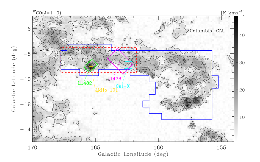
Figure 1: Integrated intensity map of the Columbia-CfA ¹²CO (J=1-0) survey towards the Galactic Plane within 154$\arcdeg$ $\leqslant l\leqslant$ 170$\arcdeg$, -15$\arcdeg$ $\leqslant b\leqslant$ -5$\arcdeg$ (from Dame et al., 2001). The integrated velocity range is from -15 to 10 km s^-1. The contours are from 10 % to 90 % by a step of 10 % of the maximum intensity value ($\sim$ 46 K km s^-1). The blue polygon marks the scanning coverage of the MWISP CO survey (Wang et al. in prep). The red dashed box indicates the region focused in this work, based on the MWISP data. The green, magenta and cyan polygons show the observed regions toward L1482 (Li et al., 2014), L1478 (Chung et al., 2019), and Cal-X (Imara et al., 2017), respectively. The plus sign represents the location of the $\mathrm{LkH}\alpha$ 101 cluster throughout all the figures in this work.

Located in the Taurus-Perseus-Auriga complex (Ungerechts & Thaddeus, 1987; Dame et al., 2001), the CMC is identified to be a giant molecular cloud (GMC), which is similar to the Orion Molecular Cloud (OMC) in mass ($\sim$ 10⁵ M_⊙) and size ($\sim$ 80 pc), but in an earlier evolution stage (Lada et al., 2009; Broekhoven-Fiene et al., 2018). Compared with the OMC, the CMC was found to contain 15$-$20 times fewer young stellar objects (YSOs) in number (Broekhoven-Fiene et al., 2014). Only one cluster LkH$\alpha$ 101 was found to be embedded in the reflection nebula NGC 1579 in the CMC (Andrews & Wolk, 2008), and the estimated age of the cluster is $\sim$ 1 Myr (Wolk et al., 2010). The Columbia-CfA 1.2 m ¹²CO (J=1-0) survey showed that the CMC is an elongated molecular cloud (see Figure 1). The $Herschel$ observations further showed filamentary structures in the CMC (Harvey et al., 2013; Lada et al., 2017), covering an area roughly from 160$\arcdeg$ to 168$\arcdeg$ along the Galactic Longitude and from -10$\arcdeg$ to 7$\arcdeg$ along the Galactic Latitude. Therefore, the CMC can serve as an ideal laboratory to investigate the structures and dynamics of large-scale filamentary gas structures and early-phase star formation therein.

In recent years, various observations have been carried out toward subregions in the CMC, such as L1482, L1478 and California-X. Li et al. (2014) investigated the kinematic and dynamical states of the L1482 nebula, the most active star formation region in the CMC, and investigated the physical properties of dense clumps by molecular line emission observations of the ¹²CO (2-1), ¹²CO (3-2), and ¹³CO (1-0). Imara et al. (2017) studied the relationship between filaments, cores, and outflows in the California-X region centered at (l, b)=(162.4$\arcdeg$, -8.8$\arcdeg$) by ¹²CO (2-1) and ¹³CO (2-1). Lada et al. (2017) provided a census of YSOs by combining the data from $IRAS$ (Lada et al., 2009), $Herschel$ (Harvey et al., 2013) and $Spitzer$ (Broekhoven-Fiene et al., 2014). Zhang et al. (2018) performed single-pointing IRAM-30 m observations of molecular lines near 90 GHz to the CMC and derived the physical properties of dense cores extracted from the $Herschel$ data. Broekhoven-Fiene et al. (2018) identified a sample of protostellar objects by the 850 $\mu$m and 450 $\mu$m observations using the SCUBA-2 as part of the JCMT Gould Belt Legacy Survey. Chung et al. (2019) performed observations of molecular lines in the frequency range of 85$-$115 GHz to study the kinematics of the filaments and chemical evolution of the dense cores toward the L1478 region. However, the studies mentioned above mainly focused on the small filamentary structures and dynamic properties in the subregions of the CMC, and there is currently a lack of study on the structure and dynamics of this molecular cloud as a whole.

The Milky Way Imaging Scroll Painting (MWISP) project is a large CO (J=1–0) multi-line survey towards the northern Galactic Plane, using the PMO-13.7 m millimeter telescope. This unbiased survey provides us a good opportunity to study large-scale filamentary molecular clouds, as well as star formation therein (see, e.g. Xiong et al., 2019). As a part of the MWISP survey, we present in this work the results of the three CO (J=1-0) isotopologue line observations toward the CMC. In Section 2, we describe the CO line observations and data reduction. We present observational results in Section 3 and discuss these results in Section 4. In Section 5, we make a summary of these discussions.

2 Observations and Data Reduction

The three CO isotopologue lines observations were simultaneously performed from February 2012 to May 2014 with the PMO-13.7 m millimeter telescope located in Delingha, China. The observations were performed using a 3$\times$3 beams sideband separation Superconducting Spectroscopic Array Receiver (SSAR) system (Shan et al., 2012). The frequency of the local oscillator (LO) was carefully selected, and thus the ${}^{12}\mathrm{CO}$ is at the upper sideband (USB), and ${}^{13}\mathrm{CO}$ and $\mathrm{C}^{18}\mathrm{O}$ are at the lower sideband (LSB), respectively. The pointing uncertainty is approximately within 5$\arcsec$. The observations were conducted by position-switch On-The-Fly (OTF) mode, and the telescope scaned the sky along both the longitude and latitude directions at a constant rate of 50$\arcsec$s^-1. Velocities were all given with respect to the local standard of rest (LSR). The observational parameters of frequency, half-power beamwidth (HPBW), velocity resolution ($\Delta\mathrm{v}$), rms noise levels ($\sigma_{\mathrm{rms}}$), typical system temperatures, and beam efficiencies ($\eta_{\rm MB}$) are listed in Table 1. For more information about the telescope, to refer to the status report of the PMO-13.7 m millimeter telescope. All data were reduced by GILDAS/CLASS package. After removing bad channels and abnormal spectra and correcting the first order (linear) baseline fitting, the data were regridded into the standard FITS files with a pixel size of 30$\arcsec\times$ 30$\arcsec$ (approximately half of the beam size).

Table 1: PMO-13.7 m observational parameters

Tracer	Frequency	HPBM	$\Delta\mathrm{v}$	Mean Noise ($\sigma_{\mathrm{rms}}$)	System Temperatures	$\eta_{\rm MB}$
	(GHz)	($\arcsec$)	(kms-1)	(K)	(K)	(K)
12CO(J=1-0)	115.271	52	0.16	0.48	$\sim$ 270	44%
13CO(J=1-0)	110.201	55	0.17	0.28	$\sim$ 175	48%
C18O(J=1-0)	109.782	55	0.17	0.28	$\sim$ 175	48%

3 Results

3.1 Overview of the CMC

As shown in Figure 1, the blue solid polygon marks the whole CMC area observed by the MWISP CO survey, which covers 37.5 square degree. In this work, we focus on the 6$\arcdeg\times$ 2$\arcdeg$ region (161.75$\arcdeg\leqslant l\leqslant$ 167.75$\arcdeg$, -9.5$\arcdeg\leqslant b\leqslant$ -7.5$\arcdeg$) as outlined by the red dashed box, which contains the filamentary structure suggested by the $Herschel$ observations (see, e.g, Harvey et al., 2013). The MWISP CO data towards the larger-scale observed region will be presented in other work (Wang et al. in prep).

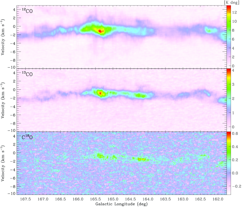
Figure 2: The LV maps of ¹²CO (upper panel), ¹³CO (middle panel), and C¹⁸O (bottom panel) toward the Galactic Plane within 161.75$\arcdeg\leqslant l\leqslant$ 167.75$\arcdeg$ and -10 kms${}^{-1}\leqslant v\leqslant$ 5 km s^-1. The Latitude is integrated from -9.5$\arcdeg$ to -7.5$\arcdeg$.

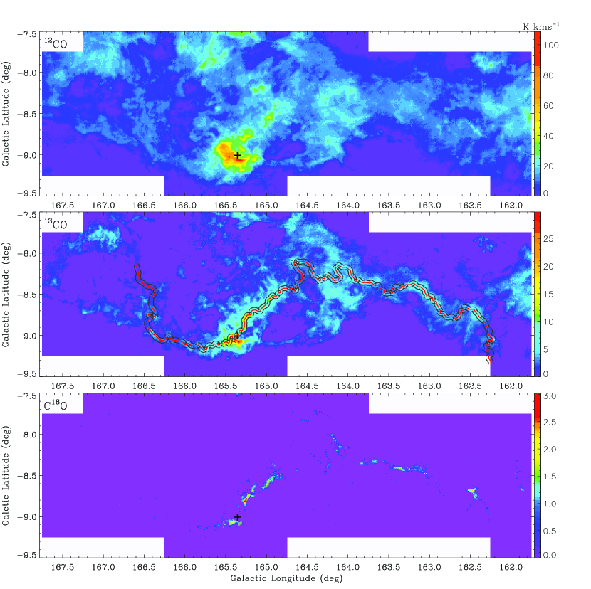
Figure 3: The panel from top to bottom is the m0 maps of ¹²CO, ¹³CO, and C¹⁸O integrated in [-10, 5] km s^-1, respectively. The unit of the colorbar is K km s^-1. The red curve in the middle panel indicate the ridgeline of the CMF with width (black dotted lines) of $0.6\,\mathrm{pc}$ $(\sim 8\,$ pixels$)$

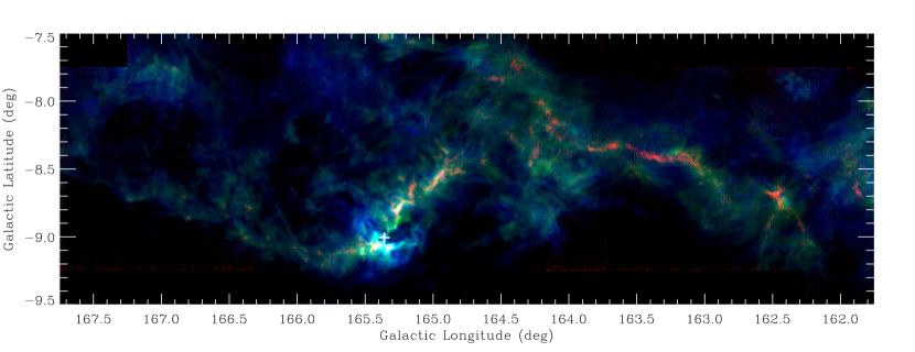
Figure 4: The three-color image of the ¹²CO (blue), ¹³CO (green), and C¹⁸O (red) emission integrated in [-10, 5] km s^-1. The intensity scales are set to be [0, 50] K km s^-1 for ¹²CO, [0, 15] K km s^-1 for ¹³CO, and [0, 1.5] K km s^-1 for C¹⁸O, respectively.

In the Columbia-CfA ¹²CO (J=1-0) survey, the velocity distribution of the CMC is mainly in the range of $\sim$ [-15, 10] km s^-1 (see, e.g, Lada et al., 2009). Figure 2 shows the Longitude-Velocity (LV) diagram of the MWISP ¹²CO emission, the main velocity component is coherent and narrowly distributed within [-10, 5] km s^-1. It is found empirically that the typical gas densities traced by ¹²CO, ¹³CO, and C¹⁸O are $\sim$ $10^{2}$ cm^-3, $\sim$ $10^{3}$ cm^-3, and $\sim$ $10^{4}$ cm^-3, respectively (Yonekura et al., 2005). As shown in Figure 3, the ¹²CO emission distributes diffusely and peripherally in the integral intensity (m0) map integrated in [-10, 5] km s^-1. The ¹³CO emission shows the large-scale filamentary structures extending about 5$\arcdeg$ from east to west. C¹⁸O is generally found to trace dense cores. In this work, bright C¹⁸O emission also outlines the ridgeline of the filamentary structure in the CMC region. As shown in Figure 4, the three-colored intensity diagram clearly shows the relative spatial emission area and intensity traced by three isotopologue CO lines, respectively.

3.2 Physical Properties of the CMC

We adopt 470 pc as the distance of the CMC from Zucker et al. (2019) who measured the distances of molecular clouds based on the dust-extinction using the $Gaia$ DR2. Assuming the ¹²CO line is optically thick ($\tau\gg 1$), the basic physical parameters of the molecular cloud are estimated through the methods as follows. Following Garden et al. (1991), with the background temperature ${T}_{\rm bg}=2.73$ K, the excitation temperature ($T_{\rm ex}$) could be calculated from the peak temperature of the ¹²CO emission ($T_{\rm mb,peak,^{12}CO}$):

$$T_{\rm ex}=5.532\left({\rm log}(1+\frac{5.53}{T_{\rm mb,peak,^{12}CO}+0.819})\right)^{-1}~{}({\rm K}).$$ (1)

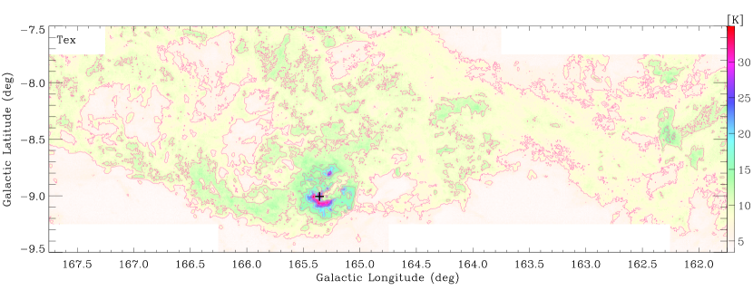
Figure 5: The excitation temperature map in the velocity interval of [-10, 5] km s^-1. The contours are set from 3.4 K to 35.0 K by a step of 10 %.

As shown in Figure 5, the excitation temperature ranges from 3.3 K to 34.9 K with a mean value of 7.8 K. The Peak value (34.9 K) appears in the position of (l, b) = (165.34$\arcdeg$, -9.08$\arcdeg$), spatially coincides with the position of the LkH$\alpha$ 101 cluster. It is comparable with the dust temperature (18-33 K; see Lada et al., 2017). The excitation temperature around the subregion L1482 ($\sim$ 15 K) is higher compared to that around L1478 ($\sim$ 8 K).

The H₂ column density can be estimated directly by integrating the main beam temperature ($T_{\rm mb}$) of ¹²CO over the velocity ($V$) using the CO-to-H₂ conversion factor $X=$ 1.8$\times$10²⁰ cm^-2 K^-1 km^-1 s from Dame et al. (2001):

$$N_{\rm H_{2}}=X\int T_{\rm mb,^{12}CO}dV.$$ (2)

Under the assumption of local thermodynamic equilibrium (LTE) and optical thin of the ¹³CO and C¹⁸O lines, given the equal excitation temperature, the column densities traced by ¹³CO and C¹⁸O can be estimated from:

$$N_{\rm{}^{13}CO}=2.42\times 10^{14}\cdot\frac{(1+0.88/T_{\rm ex})\int T_{\rm mb,^{13}CO}dV}{1-{\rm exp}(-5.29/T_{\rm ex})},\rm and$$ (3)

$$N_{\rm C^{18}O}=2.24\times 10^{14}\cdot\frac{(1+0.88/T_{\rm ex})\int T_{\rm mb,C^{18}O}dV}{1-{\rm exp}(-5.27/T_{\rm ex})}.$$ (4)

The H₂ column density could be then derived by multiplying ¹³CO column density with the ratio of $N_{\rm H_{2}}/N_{\rm{}^{13}CO}$ $\sim$ 7$\times$10⁵ (Frerking et al., 1982) or multiplying C¹⁸O column density with the ratio of $N_{\rm H_{2}}/N_{\rm C^{18}O}$ $\sim$ 7$\times$10⁶ (Castets & Langer, 1995). The pixels at least 3 channels above 3 $\sigma$ are kept in this calculation. The column density derived from ¹³CO span a range of 0.09$-$33.8 $\times 10^{21}\mathrm{~{}cm}^{-2}$, a considerably larger range than those measured by ¹²CO (0.10$-$19.6 $\times 10^{21}\mathrm{~{}cm}^{-2}$) and C¹⁸O (1.14$-$26.7 $\times 10^{21}\mathrm{~{}cm}^{-2}$). In the estimation process of mass and number density of the CMC, a mean molecular weight per H₂ molecule of 2.83 (Kauffmann et al., 2008) is adopted. The mean values are listed in Table 2.

The emission areas and the masses estimated from ¹²CO, ¹³CO, and C¹⁸O gradually decrease in quality by an order of magnitude. The low-density molecular gas traced by ¹²CO accounts for most part of the total mass, while the denser gas traced by ¹³CO and C¹⁸O is better to trace the filamentary skeletons (see below). The use of a uniform abundance ratio will lead to a deviation in the estimation of mass. Actually, the abundances may be quite different in different regions. Some studies have shown that under the assumption of optical thin and without considering the change of abundance, the mass calculated from ¹³CO may be underestimated by 2-3 times (Heyer et al., 2009; Goldsmith et al., 2008).

Table 2: Properties of the CO emission in the CMC

Emission	Velocity interval	Area	$N\rm(H_{2})$	$n\rm(H_{2})$	$M\rm(H_{2})$
	(km s-1)	(deg2)	($10^{21}$cm-2)	(cm-3)	($10^{4}$M☉)
12CO(J=1-0)	[-10, 5]	8.76	2.83 $\pm$ 0.19	67	2.59 $\pm$ 0.23
13CO(J=1-0)	[-10, 5]	4.85	2.14 $\pm$ 0.18	68	0.85 $\pm$ 0.33
C18O(J=1-0)	[-10, 5]	0.15	5.10 $\pm$ 1.84	911	0.09 $\pm$ 0.03

Note. — a, mean value with weight of integrated intensity.

3.3 Filamentary Structure

3.3.1 Major Filament

As shown in Figure 2, the ¹³CO emission distributes continuously in the velocity interval of [-5, 3] km s^-1. We calculate the column density in this velocity interval and apply for the DisPerSE algorithm (Sousbie, 2011) to extract the skeleton structures. In the process of the identification, the persistence threshold is set to be $5.8\times 10^{21}$ cm^-2 ($\sim$ 50 $\sigma$). The parameter -trimBelow used to filter noise is set to be $3.5\times 10^{20}$ cm^-2 ($\sim$ 3 $\sigma$). This setting would not only guarantee a clear skeleton construction with a highly contrast with the surrounding, but also retain the information of persistence in morphology as far as possible. As shown in Figure 3, the skeleton construction extends from 162.2$\arcdeg$ to 166.6$\arcdeg$ and shows an integral symbol-like shape. Adopting the distance of 470 pc, the length of the filament is estimated to be $\sim$ 72 pc. Hereafter, we name this filament as California Molecular Filament (CMF).

We construct the mean column density profile $N_{p}(r)$ of the CMF from radial cuts using a similar procedure as described in Arzoumanian et al. (2011) and Palmeirim et al. (2013). Applying for the Plummer-like function $N_{p}(r)=N_{\mathrm{H}_{2}}^{0}/\left[1+\left(r/R_{\mathrm{flat}}\right)^{2}\right]^{(p-1)/2}$ (Cox et al., 2016), where $N_{\mathrm{H}_{2}}^{0}$ is the amplification, $R_{\rm flat}$ is the inner flattening radius, and $p$ is the power index at large radius $\geqslant$ $R_{\rm flat}$, to the radial density profile, the $R_{\rm flat}$ is estimated to be $\sim$ 0.30 $\pm$ 0.01 pc and $p$ is $\sim$ 1.62 $\pm$ 0.01. The full width at half maxima (FWHM) of the Plummer-like profile ($2\,R_{\mathrm{flat}}\sqrt{2^{2/(p-1)}-1}$) is $\sim$ 1.73 pc, which is equivalent to $\sim$ 3 $\times$ (2 $R_{\rm flat}$). The Gaussian FWHM of the averaged ¹³CO spectrum ($\Delta V$) is $\sim$ 1.95 $\pm$ 0.22 km s^-1. The observed velocity dispersion $\sigma_{\rm obs}=\Delta V/\sqrt{8\ln 2}$ is thus to be $\sim$ 0.83 $\pm$ 0.10 km s^-1.

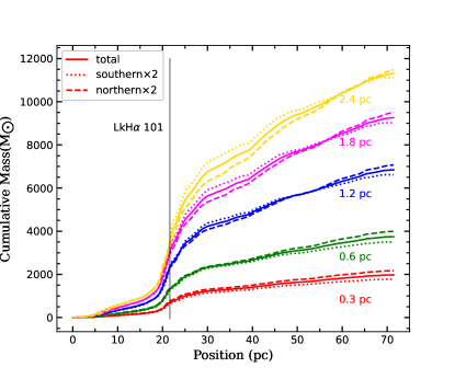
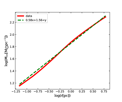
Figure 6: Left panel: The cumulative mass distribution along the CMF at different projected radii from the ridgeline, which is indicated by different colors. The profiles of southern and northern CMF multiplied by 2 are indicated by dotted and dashed lines, respectively. The LkH$\alpha$101 is indicated by vertical line. Right panel: The enclosed line-mass profile (red curves) as a function of the projected radius and the fitting line (green dashed line) in logarithmic spaces.

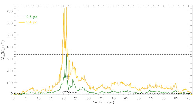
Figure 7: The $M_{\rm line}$ profiles at the projected radii of 0.6 pc (green curve) and 2.4 pc (gold curve) along the CMF. The lower and upper dashed lines show the thermal supported $M_{\rm line,crit}$ and turbulent supported $M_{\rm line,crit}$, respectively. Most parts of the CMF have $M_{\rm line}$ greater than the thermal supported $M_{\rm line,crit}$ (see the green curve), the regions around the LkH$\alpha$ 101 have $M_{\rm line}$ greater than turbulent supported $M_{\rm line,crit}$ (see the gold curve), which suggests fragmentation processes taking place along the CMF due to gravitational instability.

Similar to the Figure 6 in Álvarez-Gutiérrez et al. (2021), we show the cumulative mass profile along the CMF at the projected radii of $R_{\rm flat}$, 2$R_{\rm flat}$, 4 $R_{\rm flat}$, 6 $R_{\rm flat}$, and 8 $R_{\rm flat}$ on the north and south sides of the ridgeline respectively in Figure 6. The profiles show steep rises near the LkH$\alpha$ 101 cluster, indicating that the mass distribution along the CMF is inhomogeneous. The mass distributions are broadly symmetrical within 2$R_{\rm flat}$, being consistent with the result of Álvarez-Gutiérrez et al. (2021) for the subregion L1482. As shown in the right panel of Figure 6, the enclosed average cumulative line-mass profile along the minor axis is extracted to check the dynamic state of the CMF as a whole. By applying for a power-law fit $M_{\rm line}(r)=f\times\left(\frac{r}{\mathrm{pc}}\right)^{\gamma}$ to the profile, a power index $\gamma$ of 0.58 is derived , which is comparable with that estimated from the subregion L1482 (0.62). As shown in Figure 7, the $M_{\rm line}$ profile along the CMF at the radii of 0.6 pc and 2.4 pc are showed respectively.

Table 3: Properties of the CMF

Emission	Length	Width	Mass	$T_{\mathrm{ex}}$	$\Delta V$	$N_{\mathrm{H_{2}}}$	$M_{\mathrm{line}}$
	(pc)	(pc)	(M⊙)	(K)	(km s-1)	($10^{21}$ cm-2)	(M⊙ pc-1)
13CO	71.8	0.60 $\pm$ 0.02	1793 $\pm$ 144	10.4 $\pm$ 3.1	2.0 $\pm$ 0.2	3.64 $\pm$ 0.18	26

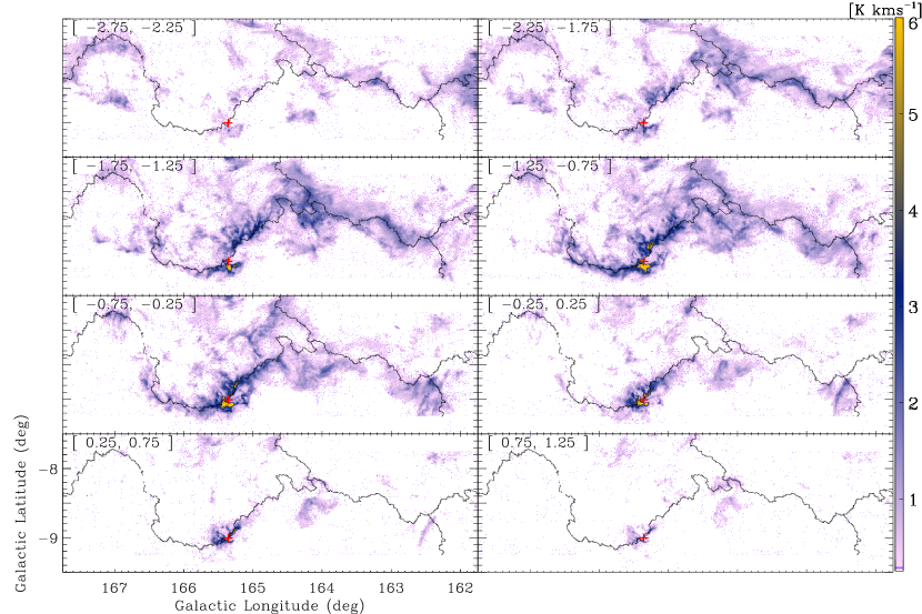
Figure 8: The ¹³CO velocity channel maps from -2.75 to 1.25 km s^-1 by a step of 0.5 km s^-1. The velocity intervals are marked in the top-left corner of each panel. The colorbar is in the unit of K km s^-1. The overlaid black lines indicate the skeleton extracted by DisPerSE. The channel maps show the kinematic of the CMC in detail.

As shown in Figure 8, the filamentary structure appears in the velocity range from -2.75 to 1.25 km s^-1. The molecular gas to the north side of the CMF mainly concentrated in the velocity of $v\textless$ -1.25 km s^-1, while the gas gather along the CMF has $v_{\rm LSR}$ range from -1.25 to 0.25 km s^-1. The western CMF ($l\textless$ 164.5$\arcdeg$) and eastern CMF ($l\textgreater$ 164.5$\arcdeg$) seem to have different systemic velocities, $\sim$ [-1.75, -0.75] km s^-1 for the eastern and $\sim$ [-1.25, -0.25] km s^-1 for the western, respectively.

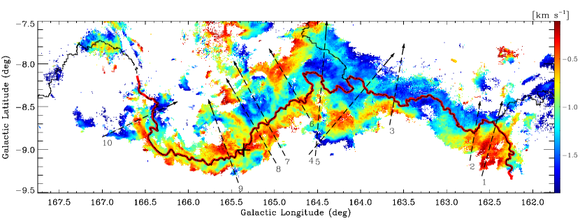
Figure 9: The m1 maps of ¹³CO in the velocity interval of [-2, 0] km s^-1. The red curve indicates the ridgeline of the CMF. The black curves are same as Figure 8. The black dashed lines perpendicular to the ridgeline are the paths of the nine PV slices.

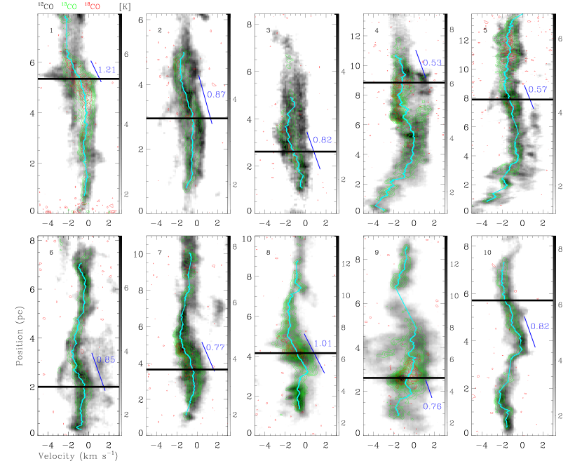
Figure 10: Ten PV plots with widths of 2 pixels along the paths indicated in Figure 9. The grayscale background, green contours, and red contours represent the ¹²CO, ¹³CO, and C¹⁸O emission, respectively. The green contours in each map are set from 3 $\sigma$ ($\sim$ 3 $\times$ 0.28 K) to peak value in an average step of 10 %. The red contours in each map are set from 1.5 $\sigma$ to peak value in an average step of 20 %. The colorbar is in the unit of K. The cyan curves indicate the ¹³CO m1 profiles. The horizontal black lines represent the positions that the CMF come cross each slice. The blue lines are the linear fitted results from the segments of m1 profiles. The corresponding fitted velocity gradients in the unit of km s^-1pc^-1 are marked besides.

In order to obtain a detailed understanding of the filament kinematics, we show the velocity distribution (m1) map of ¹³CO in [-2, 0] km s^-1 in Figure 9. The gas surrounding the integral-shaped filament is redshifted in the south side and blueshifted in the north side. As shown in Figure 10, ten PV slices are extracted across the ridgeline of the CMF. The velocity structure of ¹³CO across the major axis (horizontal black lines) is characterized by a velocity difference going from $v_{\rm LSR}$ $\sim$ -2 km s^-1 to $v_{\rm LSR}$ $\sim$ 0 km s^-1 along a length of about 1 pc. The fitted velocity gradients range from 0.66 to 1.14 km s^-1 pc^-1, with a mean value of $\sim$ 0.82 km s^-1 pc^-1.

3.3.2 Substructures

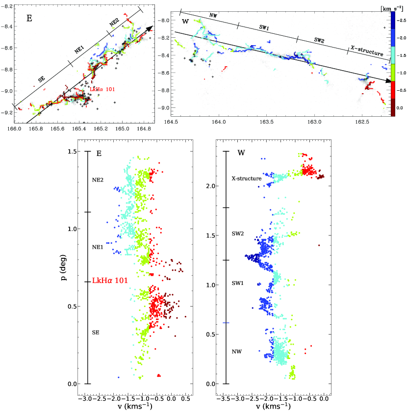
Figure 11: Upper panel: The merged skeletons (marked by different colors) extracted from the C¹⁸O emission in region E and W. Each skeleton is extracted from the channel $\mathrm{H}_{2}$ column density maps ( from -2.75 to 0.25  km s^-1 by a step of 0.5 km s^-1 with pixels above 3$\sigma$ kept) by the DisPerSE algorithm. The plus symbols indicate YSOs. The black lines indicate the extents of the regions defined in section $3.3.2$. Bottom panel: The PV plots of m1 distribution (with pixels above 3 $\sigma$ kept) in region E and W. The color setting and the extents in the black vertical lines are same as that of the upper panel.

Compared with ¹²CO and ¹³CO, the C¹⁸O emission traces the innermost structures of the molecular cloud. We try to combine the DisPerSE algorithm with the channel column density maps to resolve C¹⁸O structures. The C¹⁸O emission is detected in the region with bright ¹³CO emission, and mainly appears at $v_{\rm LSR}\sim$ -1 km s^-1 (see Figure 2 and Figure 3). The velocity resolution in the observations is $\sim$ 0.17 km s^-1, which is comparable to the isothermal sound speed in the cloud. Based on the assumption that a filament should be detected in more than three consecutive velocity channels, we estimate the channel column density every three velocity channels (0.5 km s^-1) with pixels above 3 $\sigma$ to extract the the filamentary structures. Then we merge these identified filamentary structures into a single intensity image (see Figure 11). The identified skeletons in the six velocity intervals are marked out by different colors.

As shown in Figure 11, we zoom in the Eastern ($164.7^{\circ}\leqslant l\leqslant 166^{\circ},-9.3^{\circ}\leqslant b\leqslant-8.2^{\circ}$) and Western ($162.2^{\circ}\leqslant l\leqslant 164.5^{\circ},-9.1^{\circ}\leqslant b\leqslant-7.9^{\circ}$) regions (hereafter ”E” and ”W”) and overlay the YSOs from Lada et al. (2017) on them. By the position of the cluster LkH$\alpha$ 101, E could be further divided into SE ($l\sim$ [165.5°, 166.0°]), NE1 ($l\sim$ [165.1°, 165.5°]), and NE2 ($l\sim$ [164.8°, 165.1°]), respectively. W is divided into NW ($l\sim$ [163.8°, 164.5°]), SW1 ($l\sim$ [162.6°, 163.2°]), SW2 ($l\sim$ [163.2°, 163.8°]), and X-structure ($l\sim$ [162.2°, 162.6°]), respectively. Along the directions of the arrowed lines, two PV plots are extracted from the C¹⁸O m1 map (with pixels above 3 $\sigma$). Combing the distributions of the substructures in position-position (PP) and PV spaces, we could have a better understanding of their dynamics. The C¹⁸O emission in E appears to be concentrated at -1 km s^-1 (green). The spiny structures constructed by a few pixels (maroon or cyan in SE, red or blue in NE) frequently seen along the PV plot in our study. In NE1, the emission of the substructures is blueshifted in the north side and redshifted in the south side. It can be seen that there are at least three substructures with $v_{\rm LSR}$ at -2, -1.5, and -1 km s^-1 parallel distributing within the CMF in ”zig-zag” shape. In this region, there is a distinct velocity gradient from blueshifted to redshifted towards the cluster LkH$\alpha$ 101. In NE2, more substructures are seen to overlap and merge to form hub-like features, and the YSOs in this region are more concentrated than NE1. At the western end of SE, where YSOs are the most concentrated, the substructures also present hub-like morphological features. The emission in W appears to be concentrated at -1.5 km s^-1 (cyan) and -2 km s^-1 (blue). Compared with E, fewer spiny structures appear in this region. In SW1, the substructures with $v_{\rm LSR}$ at $\sim$ -1.5, -2 km s^-1 are overlaid and their velocities are coherent in a wave form. In SW2, the substructures with $v_{\rm LSR}$ at $\sim$ -1.5 km s^-1 and $v_{\rm LSR}$ at $\sim$ -2 km s^-1 are spatially separated and their velocity distributions are more diffuse than that in SW1. In NW, the substructures appear to fragment independently of each other. For the X structure, the substructures with $v_{\rm LSR}$ at $\sim$ -2.0, -1.5 kms^-1 and $v_{\rm LSR}$ at $\sim$ -0.5, 0.0 km s^-1 are located in north and south, respectively.

3.4 Identification of Dense Cores

The theoretical models of infinite self-gravitating fluid cylinder suggest that when the line mass ($M_{\rm line}$) of an isothermal filament exceeds the critical value for equilibrium, the entire filament will collapse towards the axis and then fragment into clumps or cores (Chandrasekhar & Fermi, 1953; Ostriker, 1964; Jackson et al., 2010). By examining dense cores along filaments, one could understand the evolutionary phases of the filament and star formation therein. Thus, we use the Gaussclumps procedure in GILDAS (Stutzki & Guesten, 1990) to search for dense cores from C¹⁸O ([-4, 1] km s^-1). The threshold is set to be 0.87 K (3 $\sigma$) to ensure the completeness of the sample. Other parameters adopt the recommended values from Kramer et al. (1998). After removing the cores that with short axes less than the spatial scale (0.12 pc) and that are located at the edges of the observed region, we extract 225 C¹⁸O cores from the original sample of 5000 cores. Assuming that each core has a Gaussian-shaped density distribution both in spatial and velocity coordinates, the Gaussclumps algorithm derive the parameters of the Longitude and Latitude of Galactic coordinate system, angular sizes of the major axis and minor axis, velocity, peak temperature and line width (FWHM). By the methods as described in Gong et al. (2016), the physical properties of the dense cores including the deconvolved radius ($R\rm_{eff}$), excitation temperature ($T\rm_{ex}$), column density ($N\rm_{H_{2}}$), number density ($n\rm_{H_{2}}$), molecular cloud mass under local equilibrium ($M\rm_{LTE}$), virial mass ($M\rm_{vir}$) and virial parameter ($\alpha\rm_{vir}$ = $M\rm_{vir}$/$M\rm_{LTE}$) are derived and tabulated in Table 4.

The effective radius after deconvolution of the dense cores range from 0.02 pc to 0.28 pc with a mean value of 0.12 pc. The excitation temperatures span a range of 6.1$-$33.2 K with a mean value of 9.8 K. The number density ranges from 0.22$\times 10^{4}$ cm^-3 to 29.4$\times 10^{4}$ cm^-3 with a mean value of 1.47$\times 10^{4}$ cm^-3. The mass under local equilibrium ranges from 0.65 M_☉ to 53 M_☉ with a mean value of 4.5 M_⊙. The virial parameters span a range of 0.30$-$2.49 with a mean value of 1.15. The ratios of cores with $\alpha_{\mathrm{vir}}\textless 1$ and $\alpha_{\mathrm{vir}}\textless 2$ are approximately $41\,\%\,(93/225)$ and $96\,\%\,(215/225)$, respectively. Most of the dense cores are in gravitationally bound states. We remove 39 cores with overlapping the YSOs as well as 5 cores with associated $Herschel$ 70 $\mu$m point-sources (Stutz et al., 2013). Finally, we get 181 starless dense cores from the C¹⁸O emission. For comparison, Table 5 list the median values of the calculated physical parameters with the 95 % percentile and 5 % percentile for cores with YSOs and starless cores, respectively. The group of starless cores have a relatively lower effective radius, excitation temperature, number density, mass and a slightly larger $\alpha\rm_{vir}$ comparing to the dense cores that overlap with YSOs.

3.5 Identification of Outflow Candidates

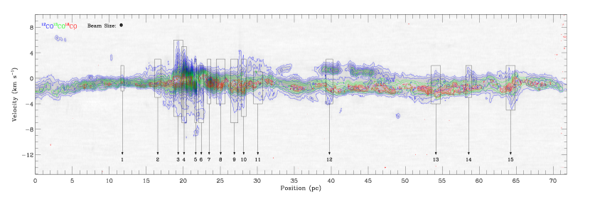
Figure 12: The PV diagram along the major axis of the CMF in the direction from east to west. The blue and green contours represent the emission of ¹²CO and ¹³CO from 3 $\sigma$ to peak value by a an average step of 3 $\sigma$. The red contours represent the emission of C¹⁸O from 1.5 $\sigma$ to peak value by a an average step of 1 $\sigma$. The black boxes mark out the positions of the protruding structures along the CMF.

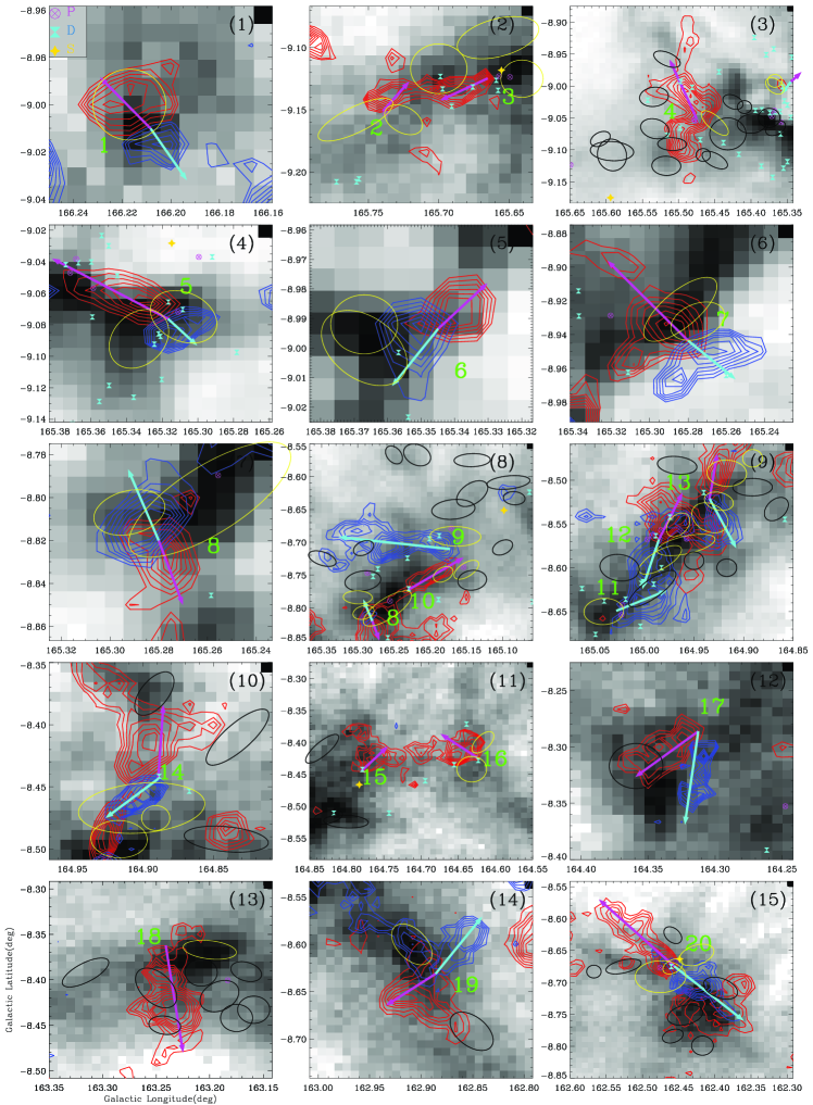
Figure 13: The 15 zoom-in regions with the red (blue) lobes as the overlaid red (blue) contours. The ID of the outflow candidates are marked besides. The background is the ¹³CO intensity map. The YSOs define P, D, S are also overlaid on each map. The ellipses are the C¹⁸O dense cores in which yellow represents the ones whose central locations are within 2.5$\arcmin$ from the driving positions of the outflow candidates and black represents the opposite.

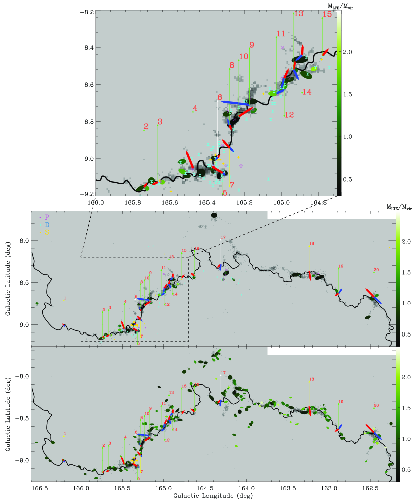
Figure 14: Upper panel: The zoomed-in area of the dashed box in the middle panel. Middle panel: The distribution of the 83 dense cores (filled ellipses) that overlap with YSOs. The dense cores are colorscaled by $\alpha\rm_{vir}$. The blueshifted lobes and redshifted lobes of the outflow candidates are simply marked by the blue and red arrows with corresponding lengths, respectively. The angle between the outflow candidate and the major axis of the CMF seems to have a random distribution. The green (yellow) arrows represent the candidates may be associated with the dense cores that overlap with YSOs (starless cores), and white represents the opposite. The YSOs are same as Figure13. The grayscale background is the C¹⁸O m0 map. Bottom panel: Same as the middle panel but for the 181 starless cores with outflow candidates overlaid.

Molecular outflow is a direct probe of star-forming activities (Arce et al., 2007). The low-J pure rotational transitions of CO have been the most used tracers of molecular outflows as it is abundant [$N$(CO) $\sim$ 10^-4 $N$(H₂)] and could be easily populated by collisions with H₂ and He at the typical densities and temperatures of molecular clouds (Bally, 2016). In order to investigate star formation along the CMF, we try to search for outflows from the ¹²CO and ¹³CO emission by checking protruding structures in the PV diagrams and mapping the spatial distribution of integrated line wings. As shown in Figure 12, there are about 15 positions (black boxes) exhibiting protruding structures which can be regarded as candidate regions for outflows. We extract the spectral lines with four pixels around the positions and estimate their center velocities $v_{\rm LSR,cen}$ as a reference of the $v\rm_{center}$ of the outflow candidates by applying for the Gaussian fitting to ¹³CO lines. Then we gradually increase velocity intervals between the $v\rm_{center}$ and the inner edges of the red or blue lobes until the extrapolated integrated intensity maps of the lobes could be distinguished from the background intensity maps. We map the integrated red or blue lobes in the 15 regions and show them in Figure 13. The average intensity of the noise level is estimated by $\sigma$(blue/red) = $\sigma\times\sqrt{V_{range}(\rm blue/red)\times 0.17}$, where $\sigma$ is the noise level and 0.17 is the velocity channel in unit of km s^-1. Lada et al. (2017) combined two extensive catalogs of YSOs in the CMC (Harvey et al., 2013; Broekhoven-Fiene et al., 2014) to provide a census of YSOs which are classified as P: protostar (Class 0/I), D: disk (Class II) and S: star (Class III). To investigate the potential origin of these outflow candidates, we overlay these YSOs on the zoomed-in maps. The Galactic coordinate, the $v\rm_{center}$, the velocity intervals of the blueshifted and redshifted lobes, the times of the integrated noise level, the center locations of the outflow candidates, the approximate boundary locations of the red (blue) lobes, and the associated YSOs in the 15 regions are listed in Table 6. As shown in Figure 13, about 20 outflow candidates with 31 individual lobes are identified. Among them, except the candidates numbered 6 and 17, the others are seen to match well with YSOs or dense cores. As shown in Figure 14, the sketch map of the distribution of these candidates shows that the angle between the outflow candidate and the major axis of the CMF seems to have a random distribution.

4 Discussions

4.1 Large-Scale Major Filament in the CMC

The CMC was firstly identified as a coherent elongated cloud at a single distance by wide-field infrared extinction maps from 2MASS (Lada et al., 2009). In the following observations toward the CMC, pc-scale filaments are identified in subregions (Li et al., 2014; Chung et al., 2019; Zhang et al., 2020). In this work, as shown in Figures 2 and 4, a 72 pc long filament extends continuously in space and velocity and stretch across these subregions. It has roughly the same length and width with ”Nessie”, the first identified large-scale massive filament, which has a length of about 80 pc and a width of 0.5 pc (Jackson et al., 2010). Based on this physical size, the typical $M_{\rm line}$ of ”Nessie” estimated from HNC (1$-$0) fluxes is $\sim$ 110 M_⊙ pc^-1 (Jackson et al., 2010). Nevertheless, Mattern et al. (2018) estimated a mean $M_{\rm line}$ of $\sim$ 627 M_⊙ pc^-1 with a physical size of 67 pc $\times$ 3 pc inferred from the near infrared data of VISTA Variables in the Via Lactea (VVV) survey and $Spitzer/GLIMPSE$ survey. The ”Nessie” Nebula contains a number of compact dense cores with a characteristic projected spacing of $\sim$ 4.5 pc. As shown in Figure 7, the $M_{\rm line}$ exceeds 100 M_⊙ pc^-1 near the cluster LkH$\alpha$ 101, with its maximum reaches $\sim$ 330 M_⊙ pc^-1 ($\sim$ 600 M_⊙ pc^-1) at the projected radii of 0.6 pc (2.4 pc). In contrast, the $M_{\rm line}$ is generally below $\sim$ 50 M_⊙ pc^-1 ($\sim$ 100 M_⊙ pc^-1) in other regions. As the CO emission traces much diffuse ISM than the submillimeter dust continuum, the $M_{\rm line}$ of the CMF may be underestimated by 2-3 times. In contrast to ”Nessie”, the mass distribution of CMF is inhomogeneous. In the traditional two-step model where thermally supercritical filaments form first and cores then form by gravitational fragmentation (Ostriker, 1964; Inutsuka & Miyama, 1992, 1997), the high line mass region of the CMF maybe created by converging flows from the low mass regions. In a high shock velocity model (Abe et al., 2020), the high line mass region can be created from the high density blobs in a short time, so the parent molecular cloud of CMF may be inhomogeneous.

Because the mass distribution is roughly symmetrical within the $R_{\rm flat}$ (see Figure 6), we use 2 $R_{\rm flat}$ (0.6 pc) as the width of the CMF to compare with the theoretical self-gravitating cylinder. The CMF has a higher mean values of the excitation temperature (10.4 $\pm$ 3.1 K) and the column density (3.64 $\pm$ 0.18 $\times$ 10²¹ cm^-2) than the CMC. The mean $M_{\rm line}$ estimated from the enclosed $M_{\rm line}$ profile (see Figure 6) is $\sim$ 26  M_⊙ pc^-1, which is larger than the critical line mass ($M_{\rm line,crit}=$ 2 $\upsilon^{2}/G\sim$ 464 $(\Delta V)^{2}\approx 16.7\,\mathrm{M}_{\odot}\mathrm{pc}^{-1}$) dominated by thermal support ($\Delta V\sim c_{s}\approx 0.19\mathrm{~{}km}\mathrm{~{}s}^{-1}$) and less than the critical line mass ($\sim$ 335.2 M_⊙ pc^-1) dominated by turbulent support ($\Delta V\sim\sigma_{tot}\approx$ 0.85 km s^-1) (see Figure 7). The detailed calculation method of the isothermal sound speed $c_{\mathrm{s}}$ and $\sigma_{tot}$ was introduced in Xiong et al. (2017, 2019). It indicates that the CMF is under the gravitationally unstable conditions and should fragment into dense cores, as we see in the C¹⁸O images. In the process, turbulent pressure can support the filament against gravitational collapse.

4.2 Kinematics of the CMF

Systematic velocity gradients across the major filament have been observed in the pc-scale filamentary structures with low line mass ($\lesssim$ 100 $\mathrm{M}_{\odot}\mathrm{pc}^{-1}$) in the regions of Serpens South, Serpens Main, NGC 1333 region (Dhabal et al., 2018), the northwestern part of the L1495 (Arzoumanian et al., 2018), B211/B213 of the Taurus cloud (Palmeirim et al., 2013; Shimajiri et al., 2019), and in the subregions of high line mass filaments ($\gtrsim$ 100 $\mathrm{M}_{\odot}\mathrm{pc}^{-1}$) such as the CMC L1482 filament (Álvarez-Gutiérrez et al., 2021) and the LBS 23 (HH24-HH26) region in Orion B (Hsieh et al., 2021).

The interpretation of the velocity gradient involves several different filament formation mechanisms, which are debated between internally-driven and externally-driven cloud and filament evolution. The numerical simulations about externally-driven formation mechanisms include, e.g. oblique MHD shock compression (Inutsuka et al., 2015; Inoue et al., 2018), colliding flows (Gómez & Vázquez-Semadeni, 2014), and direct compression of interstellar turbulence (Chen & Ostriker, 2014). The simulations from Gómez & Vázquez-Semadeni (2014) have demonstrated that filaments can be formed by colliding flows via the gravitational collapse of a molecular cloud as a whole. But such global contraction would not cause systematic velocity gradient across the major axis (Chen et al., 2020). Inutsuka et al. (2015) and Inoue et al. (2018) have argued that multiple compressions associated with expanding bubbles can create star-forming filamentary structures within sheet-like molecular cloud. Based on the MHD simulations, a similar model of anisotropic filament formation in shock-compressed layers has been proposed by Chen & Ostriker (2014). According to these models, the velocity gradient is a projection effect of the accreting material in a 2D flow within the dense layer created by colliding turbulent cells. But such simulations reproduced filaments with lower masses/line-masses comparing with the CMF. In the simulation of Abe et al. (2020), high line-mass filaments of a few pc can be created by gas flows driven by the high velocity shock wave ($v_{\mathrm{sh}}\simeq$ 10 $\mathrm{kms}^{-1}$) in a timescale of the creation of dense compressed sheet-like region, or by the compressive flow component involved in the initial turbulence at a slow shock velocity ($v_{\mathrm{sh}}\simeq$ 3 $\mathrm{kms}^{-1}$) case in a relatively longer timescale ($\gtrsim$ 2 Myr). However, the current simulations of converging flows induced by shock waves or turbulence at small scale do not support the formation of such a large-scale filament as the CMF.

Recently, Álvarez-Gutiérrez et al. (2021) analyze the CMC L1482-S filament (NE1 in this work), which has a length of $\sim$ 0.9 pc and a mean $M_{\rm line}$ of $\sim$ 205 M_⊙ pc^-1 at the projected radii of 1 pc (measured from $Herschel$ data), using IRAM multi-tracer ($\mathrm{C}^{18}\mathrm{O}(1-0),\mathrm{N}_{2}\mathrm{H}^{+}(1-0),\mathrm{HCO}^{+}(1-0),\mathrm{HNC}(1-0)$). The anti-symmetric of the radial velocity gradient of the inner portion (1.43 km s^-1pc^-1 at $r\lesssim$ 0.25 $\mathrm{pc}$, 0.17 km s^-1pc^-1 at 0.25 $\mathrm{pc}$ $\lesssim r\lesssim$ 0.4 $\mathrm{pc}$) are interpreted by solid-body rotation, which is involved in the internally-driven filament formation mechanisms. Combing the ”zig-zag” morphology and the flipped magnetic field, Álvarez-Gutiérrez et al. (2021) suggested that rotating ”corkscrew” filaments would remove inner angular momentum via the magnetic breaking, leading to collapse of the filament. The magnetic field would transport this rotational energy from small scales near the filament ridgeline to larger radii. Hsieh et al. (2021) observed a clear radial velocity gradient in the centern filament with a length of 0.16 pc of LBS 23 (HH24-HH26) region in Orion B though ALMA $\mathrm{N}_{2}\mathrm{D}^{+}$ observation. Based on the similarity between the angular momentum profile of filament and that of the dense cores or envelopes, they suggest the angular momentum of the dense circumstellar environments may be linked to the rotation of small filament. The rotation may be acquired from ambient turbulence as they did not see any evidence of large-scale flows towards the central filament and radial velocity gradients in lower-density gas maps. For the CMF, a systematic radial velocity gradient (0.82 km s^-1pc^-1) at larger radii ($\sim$ 1 pc) can be seen in Figure 9. Assuming that the rotating cylinder model is suitable for the CMF and the velocity difference between the projected radii ($r$) and the ridgeline is the rotation velocity, the angular frequency $(\omega)$ is $\sim 2.66\times 10^{-14}\mathrm{~{}s}^{-1}$, which is slightly lower than that estimated from the inner portion ($r\lesssim$ 0.25 $\mathrm{pc}$) of L1482-S filament ($4.53\times 10^{-14}\mathrm{~{}s}^{-1},$ Álvarez-Gutiérrez et al., 2021). The two comparable $\omega$ indicate the radial gradients observed at low density and outer radii and the inner high density region may correlate with each other.

The interstellar environment where the CMF is located may offer us another possibility to explain the nature of the radial velocity gradient observed in the CMF. Through inspecting the spatial distribution of the H$\alpha$ and Planck 857 GHz emission in the Taurus-Perseus region on scales up to $\geq$200 pc, Shimajiri et al. (2019) proposed an accretion model and suggested that the B211/B213 filament may have formed as a result of compression of the Per OB2 association and the Local Bubble surrounding the Sun. The distances of the Per OB2 association, Taurus cloud, and the CMC are estimated to be 340 pc (Cernis, 1993), 140 pc (Elias, 1978), and 470 pc (Zucker et al., 2019), respectively. As described in Bally et al. (2008), the most distant parts of the Taurus molecular cloud complex may be interacting with a supershell blown by the Per OB 2 association. In this picture, the Taurus cloud and the CMC may be on the front and back edge of the shell, respectively. The systematic velocity gradient across the CMF observed in this work is in a roughly opposite direction with respect to the B211/B213 filament (see, e.g. Shimajiri et al., 2019). This is consistent with the feature of the compression on the surrounding molecular clouds from the Per OB2 association. The wide-field atomic hydrogen and CO surveys towards the Per OB2 supershell and further detailed analysis about the morphology, kinematics and timescale of the Taurus-Auriga, California, and Perseus molecular clouds are presented in Chen et al. 2021. submited. They suggest that the large-scale converging supersonic flows powered by the feedback from the Per OB2 association may account for the CMF formation.

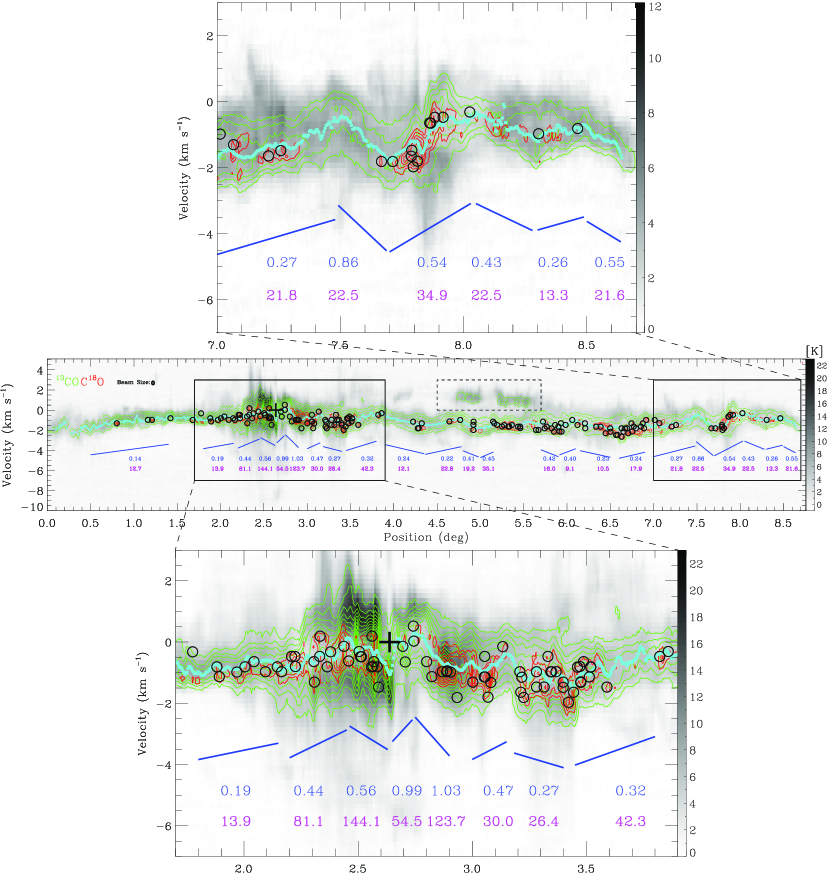
Figure 15: Top panel: Same as the middle panel but for the zoomed-in area on the west end of the CMF. Middle panel: The PV diagram along the ridgeline of the CMF with a width of 8 pixels from east to west. The grayscale background, green contours, and red contours represent the ¹²CO, ¹³CO, and C¹⁸O emission, respectively. The contours start from 3 $\sigma$ to peak value in steps of 3 $\sigma$ for ¹³CO and from 2 $\sigma$ to peak value in steps of 1 $\sigma$ for C¹⁸O , respectively. The cyan curve indicates the m1 profile of ¹³CO. In order to ensure the monotonicity of velocity component, the ¹³CO emission in the black dashed box is neglected in the m1 estimation. The blue lines indicate the linear fitted results with corresponding velocity gradients (blue) in the unit of km s^-1pc^-1 and accretion rates (magenta) in the unit of M_☉ Myr^-1 marked below. The black circles represent the extracted C¹⁸O dense cores. The solid line box marks the zoomed-in area. The colorbar is in the unit of K. Bottom panel: Same as the middle panel but for the zoomed-in area around the LkH$\alpha$ 101 cluster.

As shown in Figure 15, along the major filament, the profile of $v_{\rm LSR}$ of ¹³CO shows an oscillation pattern, which is suggested to be related to core-forming flows (see, e.g. Hacar & Tafalla, 2011; Hacar et al., 2013). All the C¹⁸O dense cores located within 0.6 pc (5 beam size) along the ridgeline are overlaid. Along the filament, we use a criterion similar to Dhabal et al. (2018) to estimated the velocity gradient, that is, if the velocity difference is greater than $0.5\mathrm{~{}km}\mathrm{~{}s}^{-1}$ (3 times velocity resolution) over a length of about 4 beam widths ($\sim$0.5 pc), the velocity gradient will be considered. Twenty-three segments are found to satisfy this criterion, their velocity gradients are estimated from the linear fitting (mpfit) of the m1 profile, and their masses are estimated from ¹³CO using the same method as in the calculation of the filament mass. Based on a simple cylindrical model from Kirk et al. (2013), the accretion rates could be estimated by $\dot{M}=\frac{\bigtriangledown V_{\shortparallel}M}{tan(\alpha)}$, here the angle of the inclination to the plane of the sky $\alpha$ is assumed to be 45°. The measured lengths, velocity differences, velocity gradients, masses, and accretion rates of the 23 segments are listed in Table 7. The mean length and mean velocity difference are $\sim$ 2.3 pc and $\sim$ 0.92 km s^-1, respectively. The accretion rates range from 9.1 to 144.1 M_☉ Myr^-1 with a mean value of 35.1 M_☉ Myr^-1.

Around the LkH$\alpha$ 101 cluster ([19, 25] pc along the CMF), the mass accretion rates are estimated to be at a magnitude of $\sim$ 101 M_☉ Myr^-1, which is about five times larger than the mean value of other regions ($\sim$ 21 M_☉ Myr^-1). In fact, as mentioned above, the mass derived from ¹³CO may be underestimated by 2-3 times, then the accretion rates here may also be underestimated. The estimated accretion rate around the LkH$\alpha$ 101 cluster is comparable with the high mass star-forming regions, e.g. Monoceros R2 (the mean accretion rate into the central hub $\sim$ 100 M_☉ Myr^-1, Treviño-Morales et al., 2019), Orion (the accretion rate per molecular finger $\sim$ 55 M_☉ Myr^-1, Hacar et al., 2017). The mean value measured in the other regions is similar to that found in low mass star formation region, e.g. Serpens South (the accretion rate at a 0.33 pc long filament $\sim$ 30 M_☉ Myr^-1; Kirk et al., 2013).

The positions of the C¹⁸O cores which hint density enhancements along the filament seem to be coupled to the oscillation patterns of the profile of $v_{\rm LSR}$. This indicates the oscillation patterns are likely formed via convergent flows caused by star formation. The fragmentation characteristic length scale ($\sim$ 2.3 pc) is comparable with that found in ”Nessie” ($\sim$ 4.5 pc). The theory of ”sausage” instability (Jackson et al., 2010) predicts that in an isothermal cylinders of finite radius $R_{\rm f}$ surrounded by an external, uniform medium, the characteristic wavelength $\lambda_{\rm{crit}}=22H$ for $R_{\rm{f}}\gg H$, while for $R_{\rm f}\ll H$, $\lambda_{\rm{crit}}=11H$, where $H=c_{\rm{s}}\left(4\pi G\rho_{\rm{c}}\right)^{-1/2}$ is the isothermal scale height. The central mass density $\rho_{\rm{c}}$ along the axis of the cylinder is $\rho_{\rm{c}}=n_{\rm{c}}\mu m_{\rm{H}}$, where $n_{\mathrm{c}}=2N_{\mathrm{c}}/\pi R_{\mathrm{flat}}$ (Liu et al., 2018). From the Plummer-like function fitting to the column density profile, $N_{\mathrm{c}}\sim$ 2.387 $\times$ 10²¹ cm^-2, which results in $\lambda_{\rm{crit}}\sim$ 1.6 pc. In the case of turbulent pressure dominates over thermal pressure, the effective scale height $H$ would become several times larger ($\sim$ 0.35 pc), then $\lambda_{\rm{crit}}\sim$ 3.9-7.8 pc. The mean fragmentation wavelength ($\sim$ 2.3 pc) along the CMF is comparable with the predictions of fragmentation of the self gravitating fluid cylinder. According to the fragmentation model of an isothermal self-gravitating gas cylinder including a helical magnetic field proposed by Nakamura et al. (1993) (see their equations 6 and 7), assuming the angle between magnetic field direction and main axis is 45$\arcdeg$, the predicted strength of the undisturbed magnetic field along directions of azimuthal and the major axis are $\sim$ 10 $\mu\mathrm{G}$ and $\sim$ 27 $\mu\mathrm{G}$, respectively. Stutz & Gould (2016) proposed a model of slingshot mechanism in which protostars are always undergoing transverse acceleration and will ”eject” from the dense filaments when they becomes sufficiently massive. They suggested the observed undulations which indicates the transverse waves propagating through the filament are magnetically induced. As shown in Figure 14 and Figure 15, the C¹⁸O cores lie close to the ridge in position and velocity. According to the slingshot mechanism, the embedded protostar system may not be massive enough to decouple from the filament, thus the CMF may at an early stage characterized by supercritical magnetism and low star formation rates (compared to Orion region, see Section 4.4) .

4.3 Substructures

Compared with the regions where the substructures are seen to overlap or roughly parallel to the major axis of the CMF (e.g. NE1, SW1), the regions where the construction of the sub-structure exhibits the hub-like features seem to contains more YSOs or more star formation activities (e.g. SE, NE2 and SW2). In NE1, the velocity gradients of the substructures are consistent with the dynamics description for the filament L1482 in Li et al. (2014), i.e., the filament might involve supersonic converging flows to feed the stellar cluster LkH$\alpha$ 101. Álvarez-Gutiérrez et al. (2021) suggested the ”zig-zag” morphology and velocity wiggles are consistent with a helical velocity field in a filament with a corkscrew-like 3D morphology. The 3D structure in this segment is explained by rotational motion about the long axis. In SW1, the wave-like velocity structures indicate accretion flows associated with cores formation. In the X-structure region, the distribution of the sub-structures is consistent with the dynamic analysis in Imara et al. (2017). As shown in the bottom panel of Figure 11, the spiny structures may be connected with the velocity gradients on beam size scale. Though as described in Clarke et al. (2018), there is very poor correspondence between the fibers in PPV space and the sub-filaments in PPP space, both the two types of structures are considered to be driven from inhomogeneities in the turbulent accretion flow onto the main filament. Similarly, we suggest that the substructures resolved in PP space and the spiny structure in PV plots may be connected with the accretion flows along sub-structures onto the ridgeline of filament.

As shown in Figure 10, there are more than one single velocity component across the CMF. In the panels 4, 5, and 6, there is a blueshifted velocity component at about -3 km s^-1 and a redshifted velocity component at about 1 km s^-1. The two velocity components seem to separate on both sides of the CMF ($v_{\rm LSR}\sim$ -1 km s^-1), which seems to be consistent with the segments shown in Figure 12 (e.g. [35, 40] pc, [40, 50] pc along the CMF). For the blueshifted velocity components, they all finally merge into the CMF. For the redshifted velocity components, they are separated from or faintly surrounding the CMF (see the panels 4, 5, 6). The multiple velocity components look like branch-like structures of the CMF. The multiple velocity components across the ridgeline of the filament may be connected with several optional origins, such as rotation (González Lobos & Stutz, 2019), cloud-envelope velocity difference, infall, or cloud-cloud collision.

4.4 Early-Phase Star Formation Activities

As described in Lada et al. (2009), the star formation activity in the CMC is significantly less than the OMC. The physical origin of the different levels of star formation activity between the two clouds may be due to the different amount of high extinction (A${}_{K}\textgreater$ 1 mag) material that the clouds contain. The CMC contains only $1\,\%$ of its mass above A_K = 1 mag, while the OMC contains roughly $10\,\%$ of its mass above the same extinction level (Lada et al., 2009). As shown in Table 2, the high density mass traced by C¹⁸O accounts for about $3.5\,\%$ of the total mass traced by ¹²CO. In the MWISP survey toward the OMC, the mass calculated from the three isotopologue lines are about 4.9$\times$10⁴ M_⊙ (¹²CO), 4.3$\times$10⁴ M_⊙(¹³CO), 0.9$\times$10⁴ M_⊙(C¹⁸O), respectively (Ma et al. in prep). The high density (C¹⁸O) mass accounts for about $18\,\%$ of the total mass (¹²CO). This ratio is significantly larger than that of the CMC.

From the PV diagram along the CMF, we have identified 20 outflow candidates with 31 individual lobes. Among them, the potential driving positions of 13 candidates are overlapped with the YSOs. As shown in Figure 13, the lobes overlap with each other. The ambiguity might be due to the interactions between the outflows, or the outflows are intrinsically weak. The investigation of outflow-filament correlation (e.g. position angle between outflows and filaments; see, e.g., Kong et al., 2019) is helpful to search for evidence of the accretion-filament correlation. For the CMF, nevertheless, see, e.g., Figure 14, the angle between the outflow candidate and the major axis of the CMF seems to have a random distribution. For a comparison, through the high spatial resolution ($\sim$ 8 $\arcsec$) observations of CO (1-0) toward the Orion A GMC (Feddersen et al., 2020), 45 protostellar outflows with 67 individual lobes were identified from an area of approximately 2 deg². The detected number per square area in the CMC ($\sim$ 2 deg^-2) is significantly less than that in the OMC ($\sim$ 20 deg^-2). On the one hand, it may be due to our insufficient resolution that cannot fully distinguish the outflow. On the other hand, it implies that stellar activity in the CMC is far less active than OMC. In addition, the line detection rate along the CMF is $\sim$ 3.5 deg^-1 in region E and 0.9 deg^-1 in region W, respectively. The western filament around L1478 contains less star formation activity and maybe in a relatively earlier stage than the eastern one around L1482.

To check the star formation activity, we present the spatial distributions of the C¹⁸O cores that overlap with YSOs and outflow candidates in Figure 14. Of these identified dense cores, $53\,\%\,(120/225)$ are distributed along the ridgeline of the CMF within a distance of 0.3 pc and $74\,\%\,(167/225)$ locate within a distance of 0.6 pc. This result is consistent with that of $Herschel$ PACS observations (Henning et al., 2010). Of the 181 starless dense cores, 94 % (171/181) have $\alpha\rm_{vir}$ less than 2 and 37 % (67/181) have $\alpha\rm_{vir}$ less than 1. The 67 starless dense cores with $\alpha\rm_{vir}$ less than 1 may have potential to further collapse to form protostars, which could be regarded as prestellar cores. The free collapse timescale $t_{\mathrm{ff}}=\left(\frac{3\pi}{32G\rho}\right)^{1/2}$ ($\rho$ is the median value of the number density of the gravitationally bound starless cores and is $\sim 6.3\times 10^{3}\rm cm^{-3}$) is estimated to be about 0.4 Myr. The total mass of the bound starless cores ($M_{\rm starless,bound}$) is $\sim$ 328 M_⊙. Assuming the star formation efficiency per free-fall time ($\frac{\epsilon}{f}$) is $\sim$ 1.8 % (Lada et al., 2010), the star formation rate (SFR $\sim\frac{\epsilon}{f}\times M_{\rm starless,bound}/t_{\mathrm{ff}}$) is $\sim$ 152 $\mathrm{M}_{\odot}\mathrm{Myr}^{-1}$. The present SFR estimated from YSO population by $\mathrm{SFR}=0.25N(\mathrm{YSOs})\times 10^{-6}\rm M_{\odot}\mathrm{yr}^{-1}$ (Lada et al., 2010) is $\sim$ 44 $\mathrm{M}_{\odot}\mathrm{Myr}^{-1}$. The sample indicates the SFR of California may increase in the future.

As shown in Figure 14, the average distance to the CMF ridgeline is $\sim$ 0.57 pc for the group of dense cores that overlap with YSOs (upper panel) and $\sim$ 0.88 pc for the group of starless cores (bottom panel), respectively. The positional correlation between cores and the ridgeline is weaker for starless cores than for the dense cores that overlap with YSOs. This may imply that star formation occurs primarily along the major filament (André et al., 2013) and then begins outside. Among the 20 outflow candidates, 15 candidates may be associated with the dense cores with YSOs (as marked by green arrows) and 3 may be associated with starless cores (as marked by yellow arrows). Thus, most (18/20) outflow candidates we identified in this work are associated with dense cores or YSOs and can be considered relatively reliable.

5 Conclusions

Based on the wide-field CO (J=1-0) isotopologue lines observations with the PMO-13.7 m millimeter telescope, we investigate the physical properties of the molecular gas in the CMC region. The main results are summarized as follows:

1, According to the space and velocity coherence, we find a large-scale filamentary molecular cloud (named as CMF in this work) with a length of about 72 pc from the ¹³CO emission. The mean line mass within the width of 0.6 pc of the CMF is estimated to be 26 M_⊙ pc^-1. Comparing with the critical line masses, the CMF is under the gravitationally unstable conditions and fragments into dense cores.

2, The CMF is found to show systematic velocity gradients perpendicular to the major axis. By checking the PV diagrams across the CMF, the typical systematic velocity gradient is estimated to be $\sim$ 0.82 km s^-1pc^-1. The potential origin including filament rotation and compression by large-scale converging flows driven by stellar feedback from the Per OB2 association are discussed.

3, Along the CMF, the large-scale velocity profile shows an oscillation pattern with a mean wavelength of $\sim$ 2.3 pc, which appears to follow the predictions of the ”sausage” instability theory. The oscillatory pattern is consistent with the kinematic model of core-forming motions, and the accretion rates are estimated to be about $\sim$ 101 M_☉ Myr^-1 around the LkH$\alpha$ 101 cluster, and $\sim$ 21 M_☉ Myr^-1 in other regions. The magnitudes of the two rates are in agreement with the estimated rates of high and low star formation in other studies, respectively.

4, Combing the C¹⁸O channel maps and the DisPerSE algorithm, substructures with slight velocity difference along the CMF are resolved. There are multiple velocity components displaying branch-like structures in some segments of the CMF. The dynamic of the substructures and the multiple velocity components along the CMF may be connected with the formation scenario of converging flows for filaments.

5, We identify a total of 225 C¹⁸O dense cores with a mean size of 0.12 pc and a mean mass of 3.3 M_⊙ in the CMC region. Of the 225 dense cores, 181 are found to have no association with YSOs. Of the 181 starless dense cores, $94\,\%\,(171/181)$ have $\alpha_{\text{vir}}$ less than 2 and $37\,\%\,(67/181)$ have $\alpha_{\text{vir}}$ less than 1. We find 20 outflow candidates with 31 individual lobes along the CMF. The detection rate of the outflow candidates in eastern CMF is higher than that in western CMF. Combining the distributions of C¹⁸O dense cores, YSOs and outflow candidates, we find there are 18 candidates may be related to C¹⁸O dense cores or YSOs, which can be considered relatively reliable. Based on these results, intense early phase star formation activity is revealed in the CMC region.

Table 4: Properties of the identified dense cores

Cores	$\Theta_{\mathrm{maj}}$	$\Theta_{\mathrm{min}}$	$PA$	$v_{\rm LSR}$	$\Delta V$	$R\rm_{eff}$	$T\rm_{ex}$	$N\rm_{H_{2}}$	$n\rm_{H_{2}}$	$M_{\mathrm{LTE}}$	$M_{\mathrm{vir}}$	$\alpha_{\mathrm{vir}}$
	($\arcmin$)	($\arcmin$)	($\arcdeg$)	(km s-1)	(km s-1)	(pc)	(K)	($10^{21}$cm-2)	($10^{3}$cm-3)	(M☉)	(M☉)
$(1)$	$(2)$	$(3)$	$(4)$	$(5)$	$(6)$	$(7)$	$(8)$	$(9)$	$(10)$	$(11)$	$(12)$	$(13)$
MWISP G165.259-8.801	1.73	4.98	53.20	-0.94	0.63	0.19	20.72	13.11	26.98	53.1	15.70	0.30
MWISP G165.333-9.089	1.75	2.48	33.20	-0.80	0.67	0.13	30.54	14.03	49.32	28.6	11.81	0.41
MWISP G165.432-9.075	2.73	2.72	0.00	-0.62	0.65	0.17	16.88	7.64	17.38	26.8	15.40	0.57
MWISP G163.682-8.327	4.59	2.35	12.40	-2.13	0.44	0.21	7.59	2.96	5.24	15.1	8.69	0.58
MWISP G165.165-8.691	1.86	4.12	91.80	-1.14	0.57	0.18	11.56	5.24	11.68	18.9	12.04	0.64
MWISP G162.475-8.691	3.96	2.93	-1.60	-1.47	0.69	0.22	8.14	4.88	8.25	26.6	22.21	0.83
MWISP G164.984-8.591	1.46	2.90	55.60	-1.47	0.57	0.12	11.34	4.23	15.12	8.5	8.45	1.00
MWISP G164.925-8.524	1.34	1.63	107.10	-1.97	0.62	0.08	12.47	5.18	40.88	5.3	6.16	1.15
MWISP G164.149-8.200	2.61	2.76	31.40	-1.49	0.39	0.17	11.04	3.09	7.20	10.5	5.44	0.52
MWISP G163.400-8.407	6.80	2.60	-5.90	-1.65	0.55	0.28	9.08	3.94	5.16	32.9	17.71	0.54

Note. — Table 4 is published in its entirety in the machine-readable format. A portion is shown here for guidance regarding its form and content.

Table 5: Median values of the properties of the dense cores

dense cores	$R_{\rm eff}$	$T\rm_{ex}$	$N\rm_{H_{2}}$	$n\rm_{H_{2}}$	$M\rm_{LTE}$	$M\rm_{vir}$	$\alpha\rm_{vir}$
	(pc)	(K)	($10^{21}$ cm-2)	($10^{3}$ cm-3)	(M⊙)	(M⊙)
all the dense cores	$0.11^{+0.08}_{-0.06}$	$9.8^{+9.7}_{-2.3}$	$1.69^{+3.4}_{-0.8}$	$7.9^{+36.7}_{-4.8}$	$3.0^{+10.6}_{-2.0}$	$3.4^{+5.8}_{-2.3}$	$1.11^{+0.85}_{-0.53}$
cores with YSOs	$0.12^{+0.13}_{-0.04}$	$10.6^{+19.8}_{-2.6}$	$2.41^{+6.3}_{-1.2}$	$8.8^{+35.0}_{-5.5}$	$5.6^{+22.8}_{-4.3}$	$5.8^{+9.9}_{-4.3}$	$0.93^{+0.79}_{-0.48}$
starless cores	$0.10^{+0.07}_{-0.05}$	$9.4^{+5.4}_{-1.9}$	$1.60^{+1.9}_{-0.7}$	$7.7^{+37.0}_{-4.6}$	$2.8^{+6.3}_{-1.8}$	$3.2^{+4.6}_{-2.1}$	$1.13^{+0.90}_{-0.46}$

Table 6: Identification of the outflow candidates

NO.	$l_{\rm zoom}$	$b_{\rm zoom}$	$z_{\rm zoom}$	$v\rm_{center}$	$v\rm_{range}$(blue)	$v\rm_{range}$(red)	$n\times\sigma\rm_{blue}$	$n\times\sigma\rm_{red}$	ID	$l$	$b$	$l_{\rm red}$	$b_{\rm red}$	$l_{\rm blue}$	$b_{\rm blue}$	YSOs
	($\arcdeg$)	($\arcdeg$)	($\arcdeg$)	(km s-1)	(km s-1)	(km s-1)				($\arcdeg$)	($\arcdeg$)	($\arcdeg$)	($\arcdeg$)	($\arcdeg$)	($\arcdeg$)	(P, D, S)
$(1)$	$(2)$	$(3)$	$(4)$	$(5)$	$(6)$	$(7)$	$(8)$	$(9)$	$(10)$	$(11)$	$(12)$	$(13)$	$(10)$	$(11)$	$(12)$	$(13)$
(1)	166.202	-9.000	0.08	0	[ -2 , 0]	[ 1 , 2]	33	10	1	166.208	-9.010	166.229	-8.988	166.193	-9.032
(2)	165.710	-9.146	0.15	0	[ -3 , -2]	[ 1 , 3]	14	14	2	165.740	-9.151	165.721	-9.127	nan	nan	P
									3	165.665.	-9.125	165.699	-9.142	nan	nan	P or D
(3)	165.493	-9.030	0.30	-1	[ -6 , -3]	[ 3 , 6]	25	10	4	165.475.	-9.050	165.512	-8.959	nan	nan	P
(4)	165.320	-9.080	0.11	-1	[ -7 , -2]	[ 2.2, 5]	40	9	5	165.317	-9.076	165.382	-9.038	165.300	-9.093	P or D
(5)	165.350	-8.990	0.06	-1	[ -7 , -2]	[ 1 , 3]	35	47	6	165.345	-8.993	165.330	-8.978	165.359	-9.013
(6)	165.285	-8.930	0.11	-1	[ -7 , -2]	[ 1 , 2]	35	45	7	165.280	-8.944	165.322	-8.896	165.255	-8.966
(7)	165.280	-8.820	0.08	-1	[ -4 , -2]	[ 1.5, 3]	16	9	8	165.280	-8.820	165.270	-8.850	165.293	-8.787
(8)	165.210	-8.700	0.30	-1.5	[ -4 , -3]	[ 1 , 3]	8	13	9	165.173	-8.710	nan	nan	165.326	-8.692	D
									10	165.231	-8.773	165.154	-8.723	nan	nan	D
(9)	164.960	-8.570	0.22	-2	[ -7 , -5]	[ 2 , 3]	5	8	11	165.028	-8.649	nan	nan	164.977	-8.623	P or D
									12	164.985	-8.568	164.962	-8.514	165.002	-8.620	P or D
									13	164.934	-8.521	164.927	-8.470	164.907	-8.578	P or D
(10)	164.887	-8.430	0.15	-1.2	[ -6 , -4]	[ 2 , 3]	4	13	14	164.889	-8.444	164.886	-8.384	164.927	-8.475	D
(11)	164.700	-8.428	0.30	-1	[ -4 , -2]	[ 0 , 1]	24	30	15	164.780	-8.445	164.745	-8.406	nan	nan	D
									16	164.625	-8.423	164.674	-8.387	nan	nan	D
(12)	164.325	-8.312	0.16	-2	[ -4 , -3]	[ 2 , 3]	13	15	17	164.313	-8.286	164.360	-8.327	164.323	-8.369
(13)	164.243	-8.400	0.20	-1.5	[ -4 , -3]	[ 0 , 2]	25	15	18	163.241	-8.362	163.225	-8.480	nan	nan
(14)	162.900	-8.635	0.20	0	[ -3 , -2]	[ 1 , 2]	15	5	19	162.886	-8.631	162.934	-8.665	162.841	-8.571
(15)	162.448	-8.692	0.30	-1	[ -5 , -3]	[ 0 , 2]	15	5	20	162.456	-8.675	162.560	-8.570	162.360	-8.760	P or D

Table 7: Properties of the segments along the major filament

Segment	Length	Velocity difference	Velocity gradient	Mass	Accretion rate
(pc, pc)	(pc)	(km s-1)	(km s-1 pc-1)	(M⊙)	(M☉ Myr-1)
(4.1 , 11.5)	7.4	1.45	0.14	87.4	12.7
(14.8 , 17.6)	2.9	0.61	0.19	73.2	13.9
(18.0 , 20.1)	2.1	1.08	0.44	179.6	81.1
(20.2 , 21.6)	1.4	1.03	0.56	251.5	144.1
(21.7 , 22.5)	0.7	0.96	0.99	54.1	54.5
(22.6 , 23.8)	1.2	1.07	1.03	118.0	123.7
(24.6 , 25.8)	1.2	0.62	0.47	62.6	30.0
(26.1 , 27.9)	1.8	0.69	0.27	95.8	26.4
(28.3 , 31.2)	2.9	1.21	0.32	128.0	42.3
(32.0 , 35.7)	3.7	1.09	0.24	48.6	12.1
(35.8 , 39.2)	3.4	0.69	0.22	99.6	22.8
(39.4 , 40.9)	1.5	0.64	0.41	45.4	19.2
(41.0 , 42.2)	1.2	0.61	0.45	76.4	35.1
(46.8 , 48.4)	1.6	0.6	0.42	37.8	16.0
(48.5 , 50.0)	1.5	0.78	0.40	22.4	9.1
(50.4 , 53.3)	2.9	0.95	0.23	45.1	10.5
(54.1 , 56.6)	2.5	0.73	0.24	72.4	17.9
(57.4 , 61.4)	3.9	1.27	0.27	79.5	21.8
(61.4 , 63.1)	1.6	1.3	0.86	25.7	22.5
(63.2 , 65.9)	2.7	1.42	0.54	63.0	34.9
(66.0 , 67.9)	1.9	0.99	0.43	50.7	22.5
(68.1 , 69.6)	1.5	0.51	0.26	50.5	13.3
(69.7 , 70.9)	1.1	0.95	0.55	38.4	21.6

References

- Abe et al. (2020) Abe, D., Inoue, T., Inutsuka, S.-. ichiro ., et al. 2020, arXiv:2012.02205
- Andrews & Wolk (2008) Andrews, S. M. & Wolk, S. J. 2008, Handbook of Star Forming Regions, Volume I, 390
- André et al. (2013) André, P., Könyves, V., Arzoumanian, D., et al. 2013, New Trends in Radio Astronomy in the ALMA Era: The 30th Anniversary of Nobeyama Radio Observatory, 476, 95
- André et al. (2014) André, P., Di Francesco, J., Ward-Thompson, D., et al. 2014, Protostars and Planets VI, 27. doi:10.2458/azu_uapress_9780816531240-ch002
- André et al. (2010) André, P., Men’shchikov, A., Bontemps, S., et al. 2010, A&A, 518, L102. doi:10.1051/0004-6361/201014666
- Arce et al. (2007) Arce, H. G., Shepherd, D., Gueth, F., et al. 2007, Protostars and Planets V, 245
- Arzoumanian et al. (2011) Arzoumanian, D., André, P., Didelon, P., et al. 2011, A&A, 529, L6. doi:10.1051/0004-6361/201116596
- Arzoumanian et al. (2018) Arzoumanian, D., Shimajiri, Y., Inutsuka, S.-. ichiro ., et al. 2018, PASJ, 70, 96. doi:10.1093/pasj/psy095
- Bally et al. (2008) Bally, J., Walawender, J., Johnstone, D., et al. 2008, Handbook of Star Forming Regions, Volume I, 308
- Bally (2016) Bally, J. 2016, ARA&A, 54, 491. doi:10.1146/annurev-astro-081915-023341
- Broekhoven-Fiene et al. (2018) Broekhoven-Fiene, H., Matthews, B. C., Harvey, P., et al. 2018, ApJ, 852, 73. doi:10.3847/1538-4357/aa911f
- Broekhoven-Fiene et al. (2014) Broekhoven-Fiene, H., Matthews, B. C., Harvey, P. M., et al. 2014, ApJ, 786, 37. doi:10.1088/0004-637X/786/1/37
- Castets & Langer (1995) Castets, A. & Langer, W. D. 1995, A&A, 294, 835
- Cernis (1993) Cernis, K. 1993, Baltic Astronomy, 2, 214. doi:10.1515/astro-1993-0203
- Chandrasekhar & Fermi (1953) Chandrasekhar, S. & Fermi, E. 1953, ApJ, 118, 116. doi:10.1086/145732
- Chen et al. (2020) Chen, C.-Y., Mundy, L. G., Ostriker, E. C., et al. 2020, MNRAS, 494, 3675. doi:10.1093/mnras/staa960
- Chen & Ostriker (2014) Chen, C.-Y. & Ostriker, E. C. 2014, ApJ, 785, 69. doi:10.1088/0004-637X/785/1/69
- Chung et al. (2019) Chung, E. J., Lee, C. W., Kim, S., et al. 2019, ApJ, 877, 114. doi:10.3847/1538-4357/ab12d1
- Clarke et al. (2018) Clarke, S. D., Whitworth, A. P., Spowage, R. L., et al. 2018, MNRAS, 479, 1722. doi:10.1093/mnras/sty1675
- Cox et al. (2016) Cox, N. L. J., Arzoumanian, D., André, P., et al. 2016, A&A, 590, A110. doi:10.1051/0004-6361/201527068
- Dame et al. (2001) Dame, T. M., Hartmann, D., & Thaddeus, P. 2001, ApJ, 547, 792. doi:10.1086/318388
- Dhabal et al. (2018) Dhabal, A., Mundy, L. G., Rizzo, M. J., et al. 2018, ApJ, 853, 169. doi:10.3847/1538-4357/aaa76b
- Elias (1978) Elias, J. H. 1978, ApJ, 224, 857. doi:10.1086/156436
- Feddersen et al. (2020) Feddersen, J. R., Arce, H. G., Kong, S., et al. 2020, ApJ, 896, 11. doi:10.3847/1538-4357/ab86a9
- Frerking et al. (1982) Frerking, M. A., Langer, W. D., & Wilson, R. W. 1982, ApJ, 262, 590. doi:10.1086/160451
- Garden et al. (1991) Garden, R. P., Hayashi, M., Gatley, I., et al. 1991, ApJ, 374, 540. doi:10.1086/170143
- Goldsmith et al. (2008) Goldsmith, P. F., Heyer, M., Narayanan, G., et al. 2008, ApJ, 680, 428. doi:10.1086/587166
- Gong et al. (2016) Gong, Y., Mao, R. Q., Fang, M., et al. 2016, A&A, 588, A104. doi:10.1051/0004-6361/201527334
- González Lobos & Stutz (2019) González Lobos, V. & Stutz, A. M. 2019, MNRAS, 489, 4771. doi:10.1093/mnras/stz2512
- Gómez & Vázquez-Semadeni (2014) Gómez, G. C. & Vázquez-Semadeni, E. 2014, ApJ, 791, 124. doi:10.1088/0004-637X/791/2/124
- Hacar et al. (2013) Hacar, A., Tafalla, M., Kauffmann, J., et al. 2013, A&A, 554, A55. doi:10.1051/0004-6361/201220090
- Hacar & Tafalla (2011) Hacar, A. & Tafalla, M. 2011, A&A, 533, A34. doi:10.1051/0004-6361/201117039
- Hacar et al. (2017) Hacar, A., Alves, J., Tafalla, M., et al. 2017, A&A, 602, L2. doi:10.1051/0004-6361/201730732
- Harvey et al. (2013) Harvey, P. M., Fallscheer, C., Ginsburg, A., et al. 2013, ApJ, 764, 133. doi:10.1088/0004-637X/764/2/133
- Henning et al. (2010) Henning, T., Linz, H., Krause, O., et al. 2010, A&A, 518, L95. doi:10.1051/0004-6361/201014635
- Heyer et al. (2009) Heyer, M., Krawczyk, C., Duval, J., et al. 2009, ApJ, 699, 1092. doi:10.1088/0004-637X/699/2/1092
- Hsieh et al. (2021) Hsieh, C.-H., Arce, H. G., Mardones, D., et al. 2021, ApJ, 908, 92. doi:10.3847/1538-4357/abd034
- Imara et al. (2017) Imara, N., Lada, C., Lewis, J., et al. 2017, ApJ, 840, 119. doi:10.3847/1538-4357/aa6d74
- Inoue et al. (2018) Inoue, T., Hennebelle, P., Fukui, Y., et al. 2018, PASJ, 70, S53. doi:10.1093/pasj/psx089
- Inutsuka et al. (2015) Inutsuka, S.-. ichiro ., Inoue, T., Iwasaki, K., et al. 2015, A&A, 580, A49. doi:10.1051/0004-6361/201425584
- Inutsuka & Miyama (1997) Inutsuka, S.-. ichiro . & Miyama, S. M. 1997, ApJ, 480, 681. doi:10.1086/303982
- Inutsuka & Miyama (1992) Inutsuka, S.-I. & Miyama, S. M. 1992, ApJ, 388, 392. doi:10.1086/171162
- Jackson et al. (2010) Jackson, J. M., Finn, S. C., Chambers, E. T., et al. 2010, ApJ, 719, L185. doi:10.1088/2041-8205/719/2/L185
- Kauffmann et al. (2008) Kauffmann, J., Bertoldi, F., Bourke, T. L., et al. 2008, A&A, 487, 993. doi:10.1051/0004-6361:200809481
- Kirk et al. (2013) Kirk, H., Myers, P. C., Bourke, T. L., et al. 2013, ApJ, 766, 115. doi:10.1088/0004-637X/766/2/115
- Kong et al. (2019) Kong, S., Arce, H. G., Maureira, M. J., et al. 2019, ApJ, 874, 104. doi:10.3847/1538-4357/ab07b9
- Kramer et al. (1998) Kramer, C., Stutzki, J., Rohrig, R., et al. 1998, A&A, 329, 249
- Lada et al. (2017) Lada, C. J., Lewis, J. A., Lombardi, M., et al. 2017, A&A, 606, A100. doi:10.1051/0004-6361/201731221
- Lada et al. (2009) Lada, C. J., Lombardi, M., & Alves, J. F. 2009, ApJ, 703, 52. doi:10.1088/0004-637X/703/1/52
- Lada et al. (2010) Lada, C. J., Lombardi, M., & Alves, J. F. 2010, ApJ, 724, 687. doi:10.1088/0004-637X/724/1/687
- Li et al. (2014) Li, D. L., Esimbek, J., Zhou, J. J., et al. 2014, A&A, 567, A10. doi:10.1051/0004-6361/201323122
- Liu et al. (2018) Liu, H.-L., Stutz, A., & Yuan, J.-H. 2018, MNRAS, 478, 2119. doi:10.1093/mnras/sty1270
- Lu et al. (2018) Lu, X., Zhang, Q., Liu, H. B., et al. 2018, ApJ, 855, 9. doi:10.3847/1538-4357/aaad11
- Mattern et al. (2018) Mattern, M., Kainulainen, J., Zhang, M., et al. 2018, A&A, 616, A78. doi:10.1051/0004-6361/201731778
- Molinari et al. (2010) Molinari, S., Swinyard, B., Bally, J., et al. 2010, A&A, 518, L100. doi:10.1051/0004-6361/201014659
- Nakamura et al. (1993) Nakamura, F., Hanawa, T., & Nakano, T. 1993, PASJ, 45, 551
- Ostriker (1964) Ostriker, J. 1964, ApJ, 140, 1056. doi:10.1086/148005
- Palmeirim et al. (2013) Palmeirim, P., André, P., Kirk, J., et al. 2013, A&A, 550, A38. doi:10.1051/0004-6361/201220500
- Shan et al. (2012) Shan, W., Yang, J., Shi, S., et al. 2012, IEEE Transactions on Terahertz Science and Technology, 2, 593. doi:10.1109/TTHZ.2012.2213818
- Shimajiri et al. (2019) Shimajiri, Y., André, P., Palmeirim, P., et al. 2019, A&A, 623, A16. doi:10.1051/0004-6361/201834399
- Sousbie (2011) Sousbie, T. 2011, MNRAS, 414, 350. doi:10.1111/j.1365-2966.2011.18394.x
- Stutz & Gould (2016) Stutz, A. M. & Gould, A. 2016, A&A, 590, A2. doi:10.1051/0004-6361/201527979
- Stutz et al. (2013) Stutz, A. M., Tobin, J. J., Stanke, T., et al. 2013, ApJ, 767, 36. doi:10.1088/0004-637X/767/1/36
- Stutzki & Guesten (1990) Stutzki, J. & Guesten, R. 1990, ApJ, 356, 513. doi:10.1086/168859
- Treviño-Morales et al. (2019) Treviño-Morales, S. P., Fuente, A., Sánchez-Monge, Á., et al. 2019, A&A, 629, A81. doi:10.1051/0004-6361/201935260
- Ungerechts & Thaddeus (1987) Ungerechts, H. & Thaddeus, P. 1987, ApJS, 63, 645. doi:10.1086/191176
- Wolk et al. (2010) Wolk, S. J., Winston, E., Bourke, T. L., et al. 2010, ApJ, 715, 671. doi:10.1088/0004-637X/715/1/671
- Xiong et al. (2017) Xiong, F., Chen, X., Yang, J., et al. 2017, ApJ, 838, 49. doi:10.3847/1538-4357/aa6443
- Xiong et al. (2019) Xiong, F., Chen, X., Zhang, Q., et al. 2019, ApJ, 880, 88. doi:10.3847/1538-4357/ab2a70
- Yonekura et al. (2005) Yonekura, Y., Asayama, S., Kimura, K., et al. 2005, ApJ, 634, 476. doi:10.1086/496869
- Zhang et al. (2018) Zhang, G.-Y., Xu, J.-L., Vasyunin, A. I., et al. 2018, A&A, 620, A163. doi:10.1051/0004-6361/201833622
- Zhang et al. (2020) Zhang, G.-Y., André, P., Men’shchikov, A., et al. 2020, A&A, 642, A76. doi:10.1051/0004-6361/202037721
- Zucker et al. (2019) Zucker, C., Speagle, J. S., Schlafly, E. F., et al. 2019, ApJ, 879, 125. doi:10.3847/1538-4357/ab2388
- Álvarez-Gutiérrez et al. (2021) Álvarez-Gutiérrez, R. H., Stutz, A. M., Law, C. Y., et al. 2021, ApJ, 908, 86. doi:10.3847/1538-4357/abd47c