A Locally Stable Edit Distance for Functions Defined on Merge Trees

Abstract

In this work we define a metric structure for functions defined on merge trees. The metric introduced possesses some stability properties and can be computed with a dynamical integer linear programming approach. We showcase the effectiveness of the whole framework with simulated data sets. Using functions defined on merge trees proves to be very effective in situation where other topological data analysis tools, like persistence diagrams, can not be meaningfully employed.

Keywords: Topological Data Analysis, Merge Trees, Reeb Graphs, Dendrograms, Tree Edit Distance

AMS subject classification

05C05, 05C10, 55N31, 62R40, 90C10 , 90C35, 90C39

1 Introduction

Topological Data Analysis (TDA) is the name given to an ensemble of techniques which are mainly focused on retrieving topological information from different kinds of data (Lum et al., 2013). Consider for instance the case of point clouds: the (discrete) topology of a point cloud itself is quite poor and it would be much more interesting if, using the point cloud, one could gather information about the topological space data was sampled from. Since, in practice, this is often not possible, one can still try to capture the “shape” of the point cloud. The idea of persistent homology (PH) (Edelsbrunner and Harer, 2008) is an attempt to do so: using the initial point cloud, a nested sequence of topological spaces is built, which are heavily dependent on the initial point cloud, and PH tracks along this sequence the persistence of the different topological features which appear and disappear. As the name persistent homology suggests, the topological features are understood in terms of generators of the homology groups (Hatcher, 2000) taken along the sequence of spaces. One of the fundational results in TDA is that this information can be represented by a set of points on the plane (Edelsbrunner et al., 2002; Zomorodian and Carlsson, 2005), with a point of coordinates $(x,y)$ representing a topological feature being born at time $x$ along the sequence, and disappearing at time $y$. Such representation is called persistence diagram (PD). Persistence diagrams can be given a metric structure through the Bottleneck and Wasserstein metrics, which, despite having good properties in terms of continuity with respect to perturbation of the original data (Cohen-Steiner et al., 2007, 2010), provide badly behaved metric spaces - with non unique geodesics arising in many situations. Various attempts to define tools to work in such spaces have been made (Mileyko et al., 2011; Turner et al., 2012; Lacombe et al., 2018; Fasy et al., 2014), but this still proves to be an hard problem. In order to obtain spaces with better properties - e.g. with unique means - and/or information which is vectorized, a number of topological summaries alternative to PDs have been proposed, such as: persistence landscapes (Bubenik, 2015), persistence images (Adams et al., 2017) and persistence silhouettes (Chazal et al., 2015).

All the aforementioned machinery has been successfully applied to a great number of problems in a very diverse set of scientific fields: complex shape analysis (MacPherson and Schweinhart, 2010), sensor network coverage (Silva and Ghrist, 2007), protein structures (Kovacev-Nikolic et al., 2016; Gameiro et al., 2014), DNA and RNA structures (Emmett et al., 2015; Rizvi et al., 2017), robotics (Bhattacharya et al., 2015; Pokorny et al., 2015), signal analysis and dynamical systems (Perea and Harer, 2013; Perea et al., 2015; Maletić et al., 2015), materials science (Xia et al., 2015; Kramár et al., 2013), neuroscience (Giusti et al., 2016; Lord et al., 2016), network analysis (Sizemore et al., 2015; Carstens and Horadam, 2013), and even deep learning theory (Hofer et al., 2017; Naitzat et al., 2020).

Related Works

Close to the definition of persistent homology for $0$ dimensional homology groups, lie the ideas of merge trees of functions, phylogenetic trees and hierarchical clustering dendrograms. Merge trees of functions (Pascucci and Cole-McLaughlin, 2003) describe the path connected components of the sublevel sets of a real valued function and are closely related to Reeb graphs (Shinagawa et al., 1991; Biasotti et al., 2008), representing the evolution of the level sets of a bounded Morse function (Audin et al., 2014) defined on a path connected domain. Phylogenetic trees and clustering dendrograms are very similar objects which describe the evolution of a set of labels under some similarity measure or agglomerative criterion. Both objects are widely used respectively in phylogenetic and statistics and many complete overviews can be found, for instance see Felsenstein and Felenstein (2004); Garba et al. (2021) for phylogenetic trees and Murtagh and Contreras (2017); Xu and Tian (2015) for clustering dendrograms. Informally speaking, while persistence diagrams record only that, at certain level along a sequence of topological spaces some path connected components merge, merge trees, phylogenetic trees and clustering dendrograms encode also the information about which components merge with which (Kanari et al., 2020; Curry et al., 2021). Usually tools like phylogenetic trees and clustering dendrograms are used to infer something about a fixed set of labels, for instance an appropriate clustering structure; however, we are more interested in looking at the information they carry as unlabeled objects.

In the last years a lot of research sparkled on such topics, with particular focus on defining metric structures, with the aim of employing populations of Reeb graphs or merge trees for data analysis. Different but related metrics have been proposed to compare Reeb graphs (Di Fabio and Landi, 2016; De Silva et al., 2016; Bauer et al., 2020, 2014), which have been shown to posses very interesting properties in terms of Morse functions on manifolds, connecting the combinatorial nature of Reeb Graphs with deformation-invariant characterizations of manifolds which are smooth, compact, orientable and without boundary. On the specific case of merge trees, there has been some research on their computation (Pascucci and Cole-McLaughlin, 2003) and on using them as visualization tools (wu and Zhang, 2013; Bock et al., 2017), while other works (Beketayev et al., 2014; Morozov et al., 2013) started to build frameworks to analyze sets of merge trees, mainly proposing a suitable metric structure to compare them, as do some more recent works (Gasparovic et al., 2019; Touli, 2020; Cardona et al., 2021). Some works specifically tackle the problem of finding a suitable metric structure via edit distances (Sridharamurthy et al., 2020; Wetzels et al., 2022), which however lack suitable stability properties.

The main issue with most of the proposed metrics is their computational cost, causing a lack for examples and applications also when algorithms are available (Touli and Wang, 2018). When applications and analysis are carried out due to the good computational properties (Sridharamurthy et al., 2020; Wetzels et al., 2022), either the employed metric does not have suitable properties and thus the authors must resort to a “computational solution to handle instabilities” (Sridharamurthy et al. (2020), Section 1.2), or the stability properties of the metric are not studied. Recently, Curry et al. (2022) proposed an approximation scheme for the interleaving distance between merge trees, describing a procedure to obtain suitable set of labels to turn the original unlabelled problem into a labelled one. While the computational advantages of this approach are outstanding, the reliability of the approximation is yet to be formally addressed - in Pegoraro (2021b) it is shown that in certain situations it may produce big errors. In Curry et al. (2022) the authors also propose the idea of decorated merge trees, which, philosophically, goes in the same direction of the novelties presented in this manuscript. See Section 6.0.3 for more details. Lastly, there is a recent preprint investigating structures lying in between merge trees and persistence diagrams, to avoid computational complexity while retaining some of the additional information provided by such objects (Elkin and Kurlin, 2021).

Main Contributions

In the present work we are interested in defining a way in which functions defined on different merge trees can be compared in a reasonable way. In fact, such functions can be very effective in extracting additional information from data, which help in several data analysis scenarios. The main idea behind the metric framework we present is that each function can be represented by the its restriction on the edges of the tree and thus one should compare the trees with such weights defined on the edges.

Instead of modifying the aforementioned metrics or other metrics for trees (Billera et al., 2001; Feragen et al., 2012; Wang and Marron, 2007) in order to account for function-weighted (unlabelled) trees, we follow the path of edit distances (Tai, 1979; Bille, 2005) because of the computational properties which they often possess, making them suited for dealing with unordered and unlabelled trees (Hong et al., 2017). The computational issues raised by those kind of trees are in fact a primary obstacle to designing feasible algorithms (Hein et al., 1995). We exploit the recent work of (Pegoraro, 2023), which proposes an edit distance (for general directed graphs) which adds fundamental modifications to usual tree edit distances, to take into account that such graphs arise as topological summaries and offers the possibility to attach abstract weights to their edges. Such work is also exploited in other papers (Pegoraro, 2021a; Pegoraro and Secchi, 2021) to work with merge trees. To account for the use of functions, we first present functional spaces on merge trees in a formal way, introducing a natural measure on these stratified spaces, and then we bridge between (Pegoraro, 2023) and the problem of comparing functions defined on merge trees, highlighting the consistencies and some potential drawbacks of our approach.

Outline

The paper is organized as follows. In Section 2 and Section 3 we introduce most of the definitions needed for our dissertation, starting from most recent TDA literature, and we tackle the problem of representing with a discrete summary - a merge tree - the merging pattern of the path-connected components of a filtration of topological spaces. Once merge trees are introduced, we use Section 4 to formally introduce the spaces of functions on a merge tree. In Section 5 we tackle the problem of finding a suitable metric structure to compare functions defined on different trees, exploiting Pegoraro (2023). In Section 6 we report some examples to showcase situations in which using functions defined on merge trees can be useful. We end up with some conclusions in Section 7.

The Appendix contains most of the proofs of the results, simulation studies and useful material which can help the reader in navigating through the content of the manuscript with multiple examples and additional details. The outline of such contents is presented at the beginning of the Appendix and coherently referenced through the manuscript.

2 Abstract Merge Trees

In TDA the main sources of information are sequences of homology groups with field coefficients: using different pipelines a single datum is turned into a filtration of topological spaces $\{X_{t}\}_{t\in\mathbb{R}}$, which, in turn, induces - via some homology functor with coefficients in the field $\mathbb{K}$ - a family of vector spaces with linear maps which are usually all isomorphisms but for a finite set of points in the sequence. Such objects are called (one-dimensional) persistence modules (Chazal et al., 2008). Any persistence module is then turned into a topological summary, for instance a persistence diagram, which completely classifies such objects up to isomorphisms. That is, if for two persistence modules there exists a family of linear isomorphisms giving a natural transformation between the two functors, then they are represented by the same persistence diagram. And viceversa. The first part of this work studies this very same pipeline but under the lenses of merge trees.

2.1 Preliminary Definitions

We start off by introducing the main mathematical objects of our research starting from the scientific literature surrounding these topics. In this process we also point out where there is no clear notation to be used and, in those situations, we produce new definitions, with motivations, to avoid being caught in the trap of using ambiguous terminology or overwriting existing and established notation.

First we need to formally define a filtration of topological spaces. We do so in a categorical fashion, following the most recent literature in TDA. Figure 1 illustrates some of the objects we introduce in this section.

Definition 1 (Curry et al. (2022))

A filtration of topological spaces is a (covariant) functor $X_{\operatorname*{\scalerel*{\cdot}{\bigodot}}}:\mathbb{R}\rightarrow\operatorname*{Top}$ from the poset $(\mathbb{R},\leq)$ to $\operatorname*{Top}$, the category of topological spaces with continuous functions, such that: $X_{t}\rightarrow X_{t^{\prime}}$, for $t<t^{\prime}$, are injective maps.

Example

Given a real valued function $f:X\rightarrow\mathbb{R}$ the sublevel set filtration is given by $X_{t}=f^{-1}((-\infty,t])$ and $X_{t<t^{\prime}}=i:f^{-1}((-\infty,t])\hookrightarrow f^{-1}((-\infty,t^{\prime}])$.

Example

Given a finite set $C\subset\mathbb{R}^{n}$ its the Céch filtration is given by $X_{t}=\bigcup_{c\in C}B_{t}(c)$. With $B_{t}(c)=\{x\in\mathbb{R}^{n}\mid\parallel c-x\parallel<t\}$. As before: $X_{t<t^{\prime}}=i:\bigcup_{c\in C}B_{t}(c)\hookrightarrow\bigcup_{c\in C}B_{t^{\prime}}(c)$.

Given a filtration $X_{\operatorname*{\scalerel*{\cdot}{\bigodot}}}$ we can compose it with the functor $\pi_{0}$ sending each topological space into the set of its path connected components. We recall that, according to standard topological notation, $\pi_{0}(X)$ is the set of the path connected components of $X$ and, given a continuous functions $q:X\rightarrow Y$, $\pi_{0}(q):\pi_{0}(X)\rightarrow\pi_{0}(Y)$ is defined as:

$$U\mapsto V\text{ such that }q(U)\subset V.$$

We use filtrations and path connected components to build more general objects which are often used as starting points of theoretical investigations in TDA.

Definition 2 (Carlsson and Mémoli (2013); Curry (2018))

A persistent set is a functor $S:\mathbb{R}\rightarrow\operatorname*{Sets}$. In particular, given a filtration of topological spaces $X_{\operatorname*{\scalerel*{\cdot}{\bigodot}}}$, the persistent set of components of $X_{\operatorname*{\scalerel*{\cdot}{\bigodot}}}$ is $\pi_{0}\circ X_{\operatorname*{\scalerel*{\cdot}{\bigodot}}}$.

Note that, by endowing a persistence set with the discrete topology, every persistence set can be seen as the persistence set of components of a filtration. Thus a general persistence set $S$ can be written as $\pi_{0}(X_{\operatorname*{\scalerel*{\cdot}{\bigodot}}})$ for some filtration $X_{\operatorname*{\scalerel*{\cdot}{\bigodot}}}$.

Now we want to carry on, going towards the definition of merge trees. The existing paths for giving such notion relying on the language of TDA split at the definition of persistence module. All such approaches however share similar notions of constructible persistent sets (Patel, 2018) or modules (Curry et al., 2022). We report here the definition of constructible persistent sets adapted from Patel (2018). The original definition in Patel (2018) is stated for persistent modules (as defined in Patel (2018)) and it is slightly different - see 1.

Definition 3 (Patel (2018))

A persistent set $S:\mathbb{R}\rightarrow\operatorname*{Sets}$ is constructible if there is a finite collection of real numbers $\{t_{1}<t_{2}<\ldots<t_{n}\}$ such that:

• $S(t<t^{\prime})=\emptyset$ for all $t<t_{1}$;

• for $t,t^{\prime}\in(t_{i},t_{i+1})$ or $t,t^{\prime}>t_{n}$, with $t<t^{\prime}$, then $S(t<t^{\prime})$ is bijective.

The set $\{t_{1}<t_{2}<\ldots<t_{n}\}$ is called critical set and $t_{i}$ are called critical values. If $S(t)$ is always a finite set, then $S$ is a finite persistent set.

Remark 1

In literature there is not an univocal way to treat critical values: in De Silva et al. (2016), Definition 3.3, constructibility conditions are stated in terms of open intervals (due to the use of cosheaves), in Patel (2018), Definition 2.2, all the conditions are stated in terms of half-closed intervals $[t_{i},t_{i+1})$, while Curry et al. (2022) differentiates between the open interval $(t_{n},+\infty)$ i.e. $t,t^{\prime}>t_{n}$, and the half closed intervals $[t_{i},t_{i+1})$. For reasons which will be detailed in Section 2.2, we stated all the conditions following De Silva et al. (2016), with open intervals.

At this point we highlight two different categorical approaches to obtain merge trees. Patel (2018) requires a persistence module to be a functor $F:\mathbb{R}\rightarrow C$ with $C$ being an essentially small symmetric monoidal category with images (see Patel (2018) and references therein). If then one wants to work with values in some category of vector spaces over some field $\mathbb{K}$, it is required that $F(t)$ is always finite dimensional. A merge tree, for Patel (2018), Example 2.1, is then a constructible persistence module with values in $FSet$, the category of finite sets.

Curry et al. (2022) instead, states that a persistence module is a functor $F:\mathbb{R}\rightarrow\operatorname*{Vec}_{\mathbb{K}}$, with $\operatorname*{Vec}_{\mathbb{K}}$ being the category of vector spaces over the field $\mathbb{K}$. This definition seems to be in line with the ones given by other works, especially in multidimensional persistence (see for instance Scolamiero et al. (2017) and references therein). On top of that, Curry et al. (2022) obtains a (generalized) merge tree as the display poset (see 5) of a persistent set. The constructibility condition on the persistence set then implies the merge tree to be tame.

In our work we find natural to work with objects which are functors, as the merge trees defined in Patel (2018), but we require some properties which are closer to the ones of constructible persistent sets, as in 3. Thus, mixing those definitions, we give the notion of an abstract merge tree.

Definition 4

An abstract merge tree is a persistent set $S:\mathbb{R}\rightarrow\operatorname*{Sets}$ such that there is a finite collection of real numbers $\{t_{1}<t_{2}<\ldots<t_{n}\}$ which satisfy:

• $S(t)=\emptyset$ for all $t<t_{1}$;

• $S(t)=\{\star\}$ for all $t>t_{n}$;

• if $t,t^{\prime}\in(t_{i},t_{i+1})$, with $t<t^{\prime}$, then $S(t<t^{\prime})$ is bijective.

The values $\{t_{1}<t_{2}<\ldots<t_{n}\}$ are called critical values of the tree.

If $S(t)$ is always a finite set, $S$ is a finite abstract merge tree.

Assumption 1

From now on we will be always working with finite abstract merge trees and, to lighten the notation, we assume any abstract merge tree to be finite, without explicit reference to its finiteness.

We point out that two abstract merge trees $\pi_{0}(X_{\operatorname*{\scalerel*{\cdot}{\bigodot}}})$ and $\pi_{0}(Y_{\operatorname*{\scalerel*{\cdot}{\bigodot}}})$ are isomorphic if there is a natural transformation $\alpha_{t}:\pi_{0}(X_{t})\rightarrow\pi_{0}(Y_{t})$ which is bijective for every $t$. This is equivalent to having the same number of path connected components for every $t$ and having bijections which make the following square commute:

for all $t<t^{\prime}$.

We report one last definition from Curry et al. (2022) which will be needed in later sections.

Definition 5 (Curry et al. (2022))

Given a persistent set $S:\mathbb{R}\rightarrow\operatorname*{Sets}$ we define its display poset as:

$$D_{S}:=\bigcup_{t\in\mathbb{R}}S(t)\times\{t\}.$$

The set $D_{S}$ can be given a partial order with $(a,t)\leq(b,t)$ if $S(t\leq t^{\prime})(a)=b$.

Given a persistent set $S$ and its display poset $D_{S}$ we define $h((a,t))=t$ and $\pi((a,t))=a$ for every $(a,t)\in D_{S}$. From $D_{S}$ we can clearly recover $S$ via $S(t)=\pi(h^{-1}(t))$ and $S(t\leq t^{\prime})(a)=b$ with $a\leq b$. Thus the two representations are equivalent and, at any time, we will use the one which is more convenient for our purposes. Note that this construction is functorial: any natural transformation $\eta:S\rightarrow S^{\prime}$ between persistent sets, gives a map of sets $D_{\eta}:D_{S}\rightarrow D_{S^{\prime}}$ with $D_{\eta}((a,t))=(\eta_{t}(a),t)$. Clearly $D_{\eta\circ\nu}=D_{\eta}\circ D_{\nu}$.

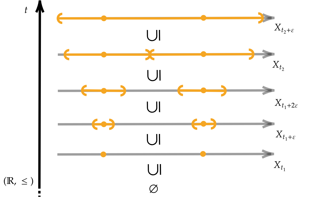
(a) A filtration $X_{\operatorname*{\scalerel*{\cdot}{\bigodot}}}$.

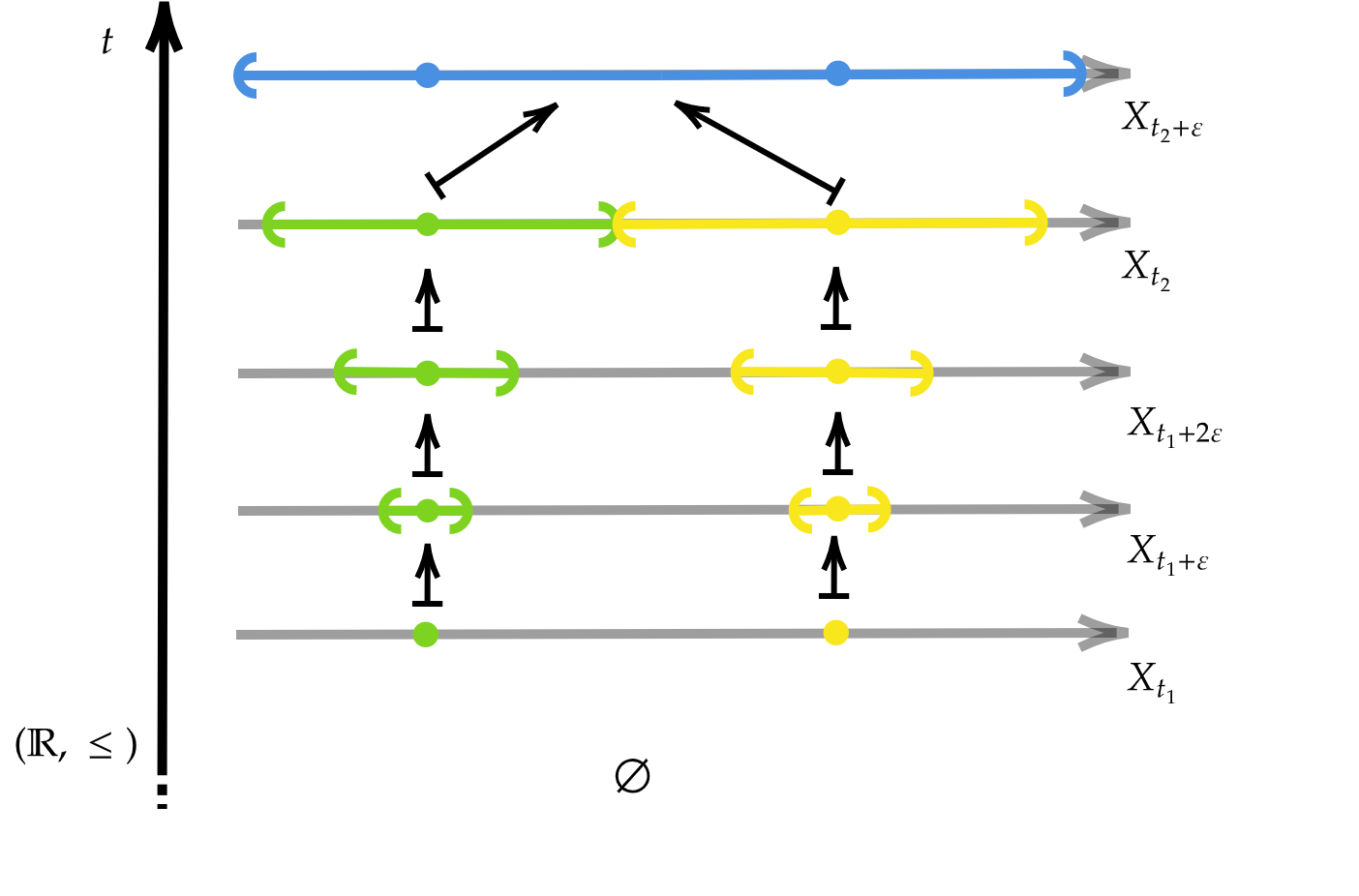
(b) The abstract merge tree $\pi_{0}(X_{\operatorname*{\scalerel*{\cdot}{\bigodot}}})$.

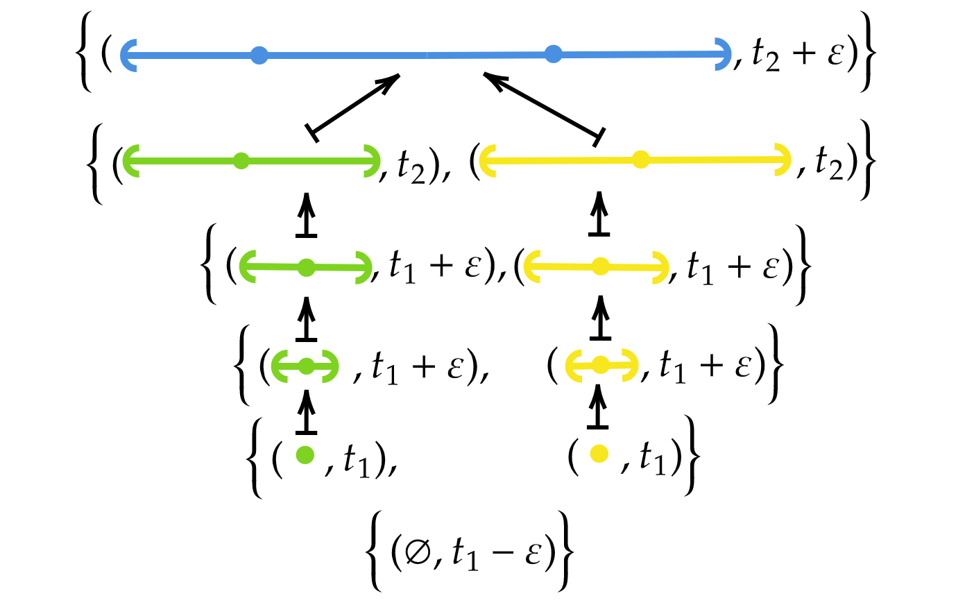
(c) The display poset $D_{\pi_{0}(X_{\operatorname*{\scalerel*{\cdot}{\bigodot}}})}$.

Figure 1: An example of a filtration along with its abstract merge tree and its display poset. The colors are used throughout the plots to highlight the relationships between the different objects.

2.2 Critical Values

Before bridging between abstract merge trees and merge trees, we need to focus on some subtle facts about critical values.

The first fact is that neither in 3 nor in 4 critical values are uniquely defined. However, thanks to the functoriality of persistence sets, we can take the intersection of all the possible sets of critical values to obtain a minimal (possibly empty) one.

Proposition 1

Let $S$ be a constructible persistence set and let $\{C_{i}\}_{i\in I}$ be a family of finite critical sets of $S$. Then $C=\bigcap_{i\in I}C_{i}$ is a critical set.

Proof  Clearly $C$ is a finite set, possibly empty. The thesis is then a consequece of the following fact: if $t\notin C$ then there is $\varepsilon>0$ such that $S(t-\varepsilon<t+\varepsilon)$ is bijective. So we can remove $t$ from any critical set of $S$ and still obtain a critical set.  

Assumption 2

Leveraging on 1, any time we take any abstract merge tree or a constructible persistent set and consider its critical values, we mean the elements of the minimal critical set.

Consider an abstract merge tree $\pi_{0}(X_{\operatorname*{\scalerel*{\cdot}{\bigodot}}})$ and let $t_{1}<t_{2}<\ldots<t_{n}$ be its (minimal set of) critical values. Let $i_{t}^{t^{\prime}}:=X_{t\leq t^{\prime}}:X_{t}\rightarrow X_{t^{\prime}}$. Given a critical value $t_{j}$, due to the minimality condition, we know that for $\varepsilon>0$ small enough, at least one between $\pi_{0}(i_{t_{j}-\varepsilon}^{t_{j}})$ and $\pi_{0}(i_{t_{j}}^{t_{j}+\varepsilon})$ is not bijective.

We want to distinguish between two scenarios:

• if $\pi_{0}(i_{t_{j}}^{t_{j}+\varepsilon})$ is bijective, we say that topological changes in the persistence set (and in the filtration) happen at $t_{j}$;

• if $\pi_{0}(i_{t_{j}}^{t_{j}+\varepsilon})$ is not bijective, we say that topological changes in the persistence set (and in the filtration) happen across $t_{j}$.

Definition 6

A constructible persistence set $\pi_{0}(X_{\operatorname*{\scalerel*{\cdot}{\bigodot}}})$ is said to be regular if all topological changes happen at its critical points.

Consider the following filtrations of topological spaces: $X_{t}=(-t,t)\bigcup(1-t,1+t)$ and $Y_{t}=[-t,t]\bigcup[1-t,1+t]$ for $t>0$ and $X_{0}=Y_{0}=\{0,1\}$. For $t<0$ the filtrations are empty. The persistent sets $\pi_{0}(X_{t})$ and $\pi_{0}(Y_{t})$ are two abstract merge trees and they share the same set of critical values, namely $\{0,1/2\}$. They only differ at the critical value $1/2$: $\pi_{0}(X_{1/2})=\{(-1/2,1/2),(1/2,1)\}$, while $\pi_{0}(X_{1/2})=\{(-1/2,1)\}$. In $X_{\operatorname*{\scalerel*{\cdot}{\bigodot}}}$ changes happen across the critical values - $\pi_{0}(X_{1/3})\cong\pi_{0}(X_{1/2})$ and $\pi_{0}(X_{1/2})\ncong\pi_{0}(X_{1})$, while in $Y_{\operatorname*{\scalerel*{\cdot}{\bigodot}}}$ changes happen at the critical values - $\pi_{0}(Y_{1/3})\ncong\pi_{0}(Y_{1/2})$ and $Y_{1/2}\cong Y_{1}$.

It is then clear that $X_{\operatorname*{\scalerel*{\cdot}{\bigodot}}}$ and $Y_{\operatorname*{\scalerel*{\cdot}{\bigodot}}}$ are not isomorphic as abstract merge trees, but, at the same time, they differ only by their behavior at critical points. We are not interested in distinguishing two such behaviours and for this reason we ask for a weaker notion of equivalence between abstract merge trees.

Given $Z\subset\mathbb{R}$, clearly $Z$ inherits an ordering from the one in $\mathbb{R}$ and we can consider $Z$ as a poset category. Thus, we can take the restriction to $Z$ of any filtration of topological spaces $X_{\operatorname*{\scalerel*{\cdot}{\bigodot}}}$ (and similarly of any persistent set) via the inclusion $Z\hookrightarrow\mathbb{R}$. We indicate this restriction as $X_{\operatorname*{\scalerel*{\cdot}{\bigodot}}\mid Z}$. Moreover, $\mathcal{L}$ is going to be the Lebesgue measure on $\mathbb{R}$. Refer to Figure 2(a) for a visual interpretation of the following definitions and propositions.

Definition 7

Two persistent sets $\pi_{0}(X_{\operatorname*{\scalerel*{\cdot}{\bigodot}}})$ and $\pi_{0}(Y_{\operatorname*{\scalerel*{\cdot}{\bigodot}}})$ are almost everywhere (a.e.) isomorphic if there is a Lebesgue measurable set $Z\subset\mathbb{R}$ such that $\mathcal{L}(\mathbb{R}-Z)=0$ and there is a natural isomorphism $\alpha:\pi_{0}(X_{\operatorname*{\scalerel*{\cdot}{\bigodot}}\mid Z})\rightarrow\pi_{0}(Y_{\operatorname*{\scalerel*{\cdot}{\bigodot}}\mid Z})$. We write $\pi_{0}(X_{\operatorname*{\scalerel*{\cdot}{\bigodot}}})\cong_{a.e}\pi_{0}(Y_{\operatorname*{\scalerel*{\cdot}{\bigodot}}})$.

Proposition 2

Being a.e. isomorphic is an equivalence relationship between persistent sets.

Proof  Reflexivity and symmetry are trivial: the first one holds with $Z=\emptyset$ and the second one holds by definition of natural isomorphism. Lastly, transitivity holds because any finite union of measure zero sets is a measure zero set.  

Now we prove that in each equivalence class of a.e. isomorphic abstract merge trees we can always pick a regular abstract merge tree, which is unique up to isomorphism.

Proposition 3

For every abstract merge tree $\pi_{0}(X_{\operatorname*{\scalerel*{\cdot}{\bigodot}}})$ there is a unique (up to isomorphism) abstract merge tree $R(\pi_{0}(X_{\operatorname*{\scalerel*{\cdot}{\bigodot}}}))$ such that:

1. $\pi_{0}(X_{\operatorname*{\scalerel*{\cdot}{\bigodot}}})\cong_{a.e.}R(\pi_{0}(X_{\operatorname*{\scalerel*{\cdot}{\bigodot}}}))$;

2. $R(\pi_{0}(X_{\operatorname*{\scalerel*{\cdot}{\bigodot}}}))$ is regular.

Regular abstract merge trees are the functors we want to focus on, for they make many upcoming definitions and results more natural and straightforward. With 3 we formally state that this choice is indeed consistent with the equivalence relationship previously established.

A more detailed discussion on the topological consequences of the regularity condition - in the particular case where $X_{\operatorname*{\scalerel*{\cdot}{\bigodot}}}$ is the sublevel set filtration of a real valued function - can be found in Pegoraro and Secchi (2021).

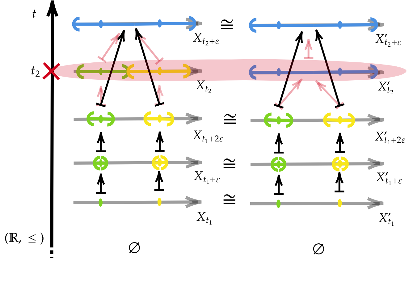
(a) An abstract merge tree $\pi_{0}(X_{\operatorname*{\scalerel*{\cdot}{\bigodot}}})$ (left) and the regular abstract merge tree $R(\pi_{0}(X_{\operatorname*{\scalerel*{\cdot}{\bigodot}}}))$ (right).

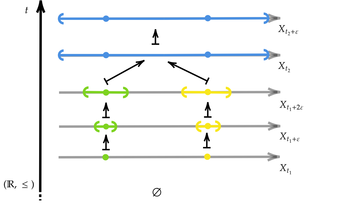
(b) A regular abstract merge tree $R(\pi_{0}(X_{\operatorname*{\scalerel*{\cdot}{\bigodot}}}))$.

(c) The merge tree $\mathcal{M}(R(\pi_{0}(X_{\operatorname*{\scalerel*{\cdot}{\bigodot}}})))$. The brackets at the end of the edges and the labels $U(p),U(q),U_{\infty}$ refer to the canonical a.e. covering defined in Section 4.2.

Figure 2: On the first line we can see an example of an abstract merge tree which is not regular (left) along with the regular abstract merge tree (right) obtained as in 3. There is also highlighted the a.e. isomorphism between them: they are isomorphic on $\mathbb{R}-\{t_{2}\}$. On the second line we find a regular abstract merge tree and the associated merge tree built as in 4. The colors are again used to highlight the relationships between the different objects.

3 Merge Trees

We introduce now the discrete counterpart of abstract merge trees, which (up to some minor technical differences) are called merge trees by part of the scientific literature dealing with these topics (Gasparovic et al., 2019; Sridharamurthy et al., 2020), while Curry et al. (2022) refers to such structures as computational merge trees. Even thou we agree with the idea behind the latter terminology, we stick with the wording used by Gasparovic et al. (2019) and others. We do so for the sake of simplicity, as these objects will be the main focus of the theoretic investigation of the manuscript. Before proceeding, we point out that there is a third approach - on top of the categorical and the computational ones - to the definition of merge trees, followed for instance by Morozov et al. (2013), which in Curry et al. (2022) is referred to as classical merge trees. We avoid dealing with such objects in our dissertation and any interested reader can find in Curry et al. (2022) how that definition relates with the other ones we report.

Now we need some graph-related definitions.

Definition 8

A tree structure $T$ is given by a set of vertices $V_{T}$ and a set of edges $E_{T}\subset V_{T}\times V_{T}$ which form a connected rooted acyclic graph. We indicate the root of the tree with $r_{T}$. We say that $T$ is finite if $V_{T}$ is finite. The order of a vertex $v_{\in}V_{T}$ is the number of edges which have that vertex as one of the extremes, and is called $ord_{T}(v)$. Any vertex with an edge connecting it to the root is its child and the root is its father: this is the first step of a recursion which defines the father and children relationship for all vertices in $V_{T}.$ The vertices with no children are called leaves or taxa and are collected in the set $L_{T}$. The relation $child<father$ generates a partial order on $V_{T}$. The edges in $E_{T}$ are identified in the form of ordered couples $(a,b)$ with $a<b$. A subtree of a vertex $v$, called $sub_{T}(v)$, is the tree structure whose set of vertices is $\{x\in V_{T}|x\leq v\}$.

Note that, given a tree structure $T$, identifying an edge $(v,v^{\prime})$ with its lower vertex $v$, gives a bijection between $V_{T}-\{r_{T}\}$ and $E_{T}$, that is $E_{T}\cong V_{T}-\{r_{T}\}$ as sets. Given this bijection, we often use $E_{T}$ to indicate the vertices $v\in V_{T}-\{r_{T}\}$, to simplify the notation.

We want to identify merge trees independently of their vertex set, and thus we introduce the following isomorphism classes.

Definition 9

Two tree structures $T$ and $T^{\prime}$ are isomorphic if exists a bijection $\eta:V_{T}\rightarrow V_{T^{\prime}}$ that induces a bijection between the edges sets $E_{T}$ and $E_{T^{\prime}}$: $(a,b)\mapsto(\eta(a),\eta(b))$. Such $\eta$ is an isomorphism of tree structures.

Finally, we give the definition of a merge tree, slightly adapted from Gasparovic et al. (2019).

Definition 10

A merge tree is a finite tree structure $T$ with a monotone increasing height function $h_{T}:V_{T}\rightarrow\mathbb{R}\cup\{+\infty\}$ and such that 1) $ord_{T}(r_{T})=1$ 2) $h_{T}(r_{T})=+\infty$ 3) $h_{T}(v)\in\mathbb{R}$ for every $v<r_{T}$.

Two merge trees $(T,h_{T})$ and $(T^{\prime},h_{T^{\prime}})$ are isomorphic if $T$ and $T^{\prime}$ are isomorphic as tree structures and the isomorphism $\eta:V_{T}\rightarrow V_{T^{\prime}}$ is such that $h_{T}=h_{T^{\prime}}\circ\eta$. Such $\eta$ is an isomorphism of merge trees. We use the notation $(T,h_{T})\cong(T^{\prime},h_{T^{\prime}})$.

With some slight abuse of notation we set $\max h_{T}=\max_{v\in V_{T}\mid v<r_{T}}h_{T}(v)$ and $\arg\max h_{T}=\max\{v\in V_{T}\mid v<r_{T}\}$. Note that, given $(T,h_{T})$ merge tree, there is only one edge of the form $(v,r_{T})$ and we have $v=\arg\max h_{T}$.

The relationship between abstract merge trees and merge trees is clarified in Section 3.1, but before going on we must introduce another equivalence relationship on merge trees.

Definition 11

Given a tree structure $T$, we can eliminate an order two vertex, connecting the two adjacent edges which arrive and depart from it. Suppose we have two edges $e=(v_{1},v_{2})$ and $e^{\prime}=(v_{2},v_{3})$, with $v_{1}<v_{2}<v_{3}$. And suppose $v_{2}$ is of order two. Then, we can remove $v_{2}$ and merge $e$ and $e^{\prime}$ into a new edge $e^{\prime\prime}=(v_{1},v_{3})$. This operation is called the ghosting of the vertex $v_{2}$. Its inverse transformation, which restores the original tree, is called a splitting of the edge $e^{\prime\prime}$.

Consider a merge tree $(T,h_{T})$ and obtain $T^{\prime}$ by ghosting a vertex of $T$. Then $V_{T^{\prime}}\subset V_{T}$ and thus we can define $h_{T^{\prime}}:=h_{T\mid V_{T^{\prime}}}$.

Now we can state the following definition.

Definition 12

Merge trees are equal up to order $2$ vertices if they become isomorphic after applying a finite number of ghostings or splittings. We write $(T,h_{T})\cong_{2}(T^{\prime},h_{T^{\prime}})$.

3.1 Regular Abstract Merge Trees and Merge Trees

In this section we study the relationship between abstract merge trees and merge trees. We collect all the important facts on this topic in the following proposition. Figure 1(b) and Figure 2(c) can help the reader going through the upcoming results.

Proposition 4

The following hold:

1. we can associate a merge tree without order $2$ vertices $\mathcal{M}(R(\pi_{0}(X_{\operatorname*{\scalerel*{\cdot}{\bigodot}}})))$ to any regular abstract merge tree $R(\pi_{0}(X_{\operatorname*{\scalerel*{\cdot}{\bigodot}}}))$;

2. we can associate a regular abstract merge tree $\mathcal{F}((T,h_{T}))$ to any merge tree $(T,h_{T})$. Moreover, we have $\mathcal{M}(\mathcal{F}((T,h_{T})))\cong_{2}(T,h_{T})$ and $\mathcal{F}(\mathcal{M}(R(\pi_{0}(X_{\operatorname*{\scalerel*{\cdot}{\bigodot}}})))\cong_{a.e.}\pi_{0}(X_{\operatorname*{\scalerel*{\cdot}{\bigodot}}})$;

3. given two abstract merge trees $X_{\operatorname*{\scalerel*{\cdot}{\bigodot}}}$ and $Y_{\operatorname*{\scalerel*{\cdot}{\bigodot}}}$, $\mathcal{M}(R(\pi_{0}(X_{\operatorname*{\scalerel*{\cdot}{\bigodot}}})))\cong\mathcal{M}(R(\pi_{0}(Y_{\operatorname*{\scalerel*{\cdot}{\bigodot}}})))$ if and only if $\pi_{0}(X_{\operatorname*{\scalerel*{\cdot}{\bigodot}}})\cong_{a.e}\pi_{0}(Y_{\operatorname*{\scalerel*{\cdot}{\bigodot}}})$.

4. given two merge trees $(T,h_{T})$ and $(T^{\prime},h_{T^{\prime}})$, we have $\mathcal{F}((T,h_{T}))\cong\mathcal{F}((T,h_{T}))$ if and only if $(T,h_{T})\cong_{2}(T^{\prime}.h_{T^{\prime}})$.

We point out an additional fact about order $2$ vertices. Suppose that we were to remove a leaf in a merge tree, the father of the deleted vertex may become an order two vertex. In case that happens, such vertex carries no topological information, since the merging that the point was representing, is no more happening (was indeed removed). And in fact the abstract merge tree associated to the merge tree with the order $2$ vertex and to the merge tree with the order $2$ vertex ghosted are the same by 4. Thus working up to order two vertices is a very natural framework to work with merge trees. And this must be taken into consideration when setting up the framework to deal with functions defined on merge trees.

The proof of 4 carries this important corollary.

Corollary 1

Given a merge tree $(T,h_{T})$ and the abstract merge tree $\pi_{0}(X_{\operatorname*{\scalerel*{\cdot}{\bigodot}}})=\mathcal{F}((T,h_{T}))$, we have $E_{T}\hookrightarrow D_{\pi_{0}(X_{\operatorname*{\scalerel*{\cdot}{\bigodot}}})}$ via $(v,v^{\prime})\mapsto(v,h_{T}(v))$.

3.2 Example of Merge Tree

Now we briefly report an example of a merge tree representing the merging structure of path-connected components along the sublevel set filtration of a function. The reader should refer to Section A for more examples, which also propel the use of merge trees over persistence diagrams.

Consider the function $f=\mid\mid x\mid-1\mid$ defined on the interval $[-2,2]$. Consider the sublevel set filtration $X_{t}=f^{-1}((-\infty,t])$. The sublevel set $X_{t}$ is an interval of the form $[-1-t,-1+t]\bigcup[1-t,1+t]$, for $t\in[0,1]$.

Consider then the abstract merge tree $\pi_{0}(X_{\operatorname*{\scalerel*{\cdot}{\bigodot}}})$. For any $t\in[0,1)$, the path connected components are $a_{t}=\{a^{t}_{1},a^{t}_{-1}\}$, with $a^{t}_{1}=[1-t,1+t]$ and $a^{t}_{-1}=[-1-t,-1+t]$ and for $t\geq 1$, $a^{t}_{2}=\{[-2,2]\}$. The critical points of the filtration are $t_{1}=0$ and $t_{2}=1$. The maps are $a_{i}^{t}\mapsto a_{i}^{t^{\prime}}$ and with $i=-1,1$, for $t\leq t^{\prime}<2$; $a_{1}^{t},a_{-1}^{t}\mapsto a_{2}^{t^{\prime}}$ for $t<2\leq t^{\prime}$ and the identity for $t,t^{\prime}\geq 2$.

The merge tree $\mathcal{M}(\pi_{0}(X_{\operatorname*{\scalerel*{\cdot}{\bigodot}}}))=(T,h_{T})$ associated to $\pi_{0}(X_{\operatorname*{\scalerel*{\cdot}{\bigodot}}})$ has a tree structure given by a root, an internal vertex and two leaves - as in Figure 2(c): if we call $v_{1}:=a^{0}_{1}$, $v_{-1}:=a^{0}_{-1}$ and $v_{2}:=a^{2}_{2}$, the merge tree $\mathcal{M}(\pi_{0}(X_{\operatorname*{\scalerel*{\cdot}{\bigodot}}}))$ is given by the vertex set $\{v_{1},v_{-1},v_{2},r_{T}\}$ and edges $e_{1}=(v_{1},v_{2})$, $e_{2}=(v_{-1},v_{2})$ and $e_{3}=(v_{2},r_{T})$. The height function has values $h_{T}(v_{1})=h_{T}(v_{-1})=t^{-}=0$, $h_{T}(v_{2})=2$ and $h_{T}(r_{T})=+\infty$.

4 Functions Defined on Display Posets

Now we formalize how we want to deal with functions defined on merge trees, devoting much care to setting up a framework in accordance with the equivalence relationships introduced in Section 2.2.

In Section 6 and Section B we make some key examples of how the framework contained in this section can be used in real data analysis scenarios to tackle problems which would be very hard to be dealt with using other topological tools. Simulated case studies can be found in Section D. Moreover, Section C focuses on why it is difficult to meaningfully replicate this framework for persistence diagrams.

4.1 Metric Spaces

Following Burago et al. (2022), we briefly report the definitions related to metric geometry that we need in the present work.

Definition 13

Let $X$ be an arbitrary set. A function $d:X\times X\rightarrow\mathbb{R}$ is a (finite) pseudo metric if for all $x,y,z\in X$ we have:

1. $d(x,x)=0$

2. $d(x,y)=d(y,x)$

3. $d(x,y)\leq d(x,z)+d(z,y)$.

The space $(X,d)$ is called a pseudo metric space.

Given a pseudo metric $d$ on $X$, if for all $x,y\in X$, $x\neq y$, we have $d(x,y)>0$ then $d$ is called a metric or a distance and $(X,d)$ is a metric space.

Proposition 5 (Proposition 1.1.5 Burago et al. (2022))

For a pseudo metric space $(X,d)$, $x\sim y$ iff $d(x,y)=0$ is an equivalence relationship and the quotient space $(X,d)/\sim$ is a metric space.

Definition 14

Consider $X,Y$ pseudo metric spaces. A function $f:X\rightarrow Y$ is an isometric embedding if it is injective and $d(x,y)=d(f(x),f(y))$. If $f$ is also bijective then it is an isometry or and isometric isomorphism.

Definition 15

A pseudo metric $d$ on $X$ induces the topology generated by the open balls $B_{\varepsilon}(x):=\{y\in X\mid d(x,y)<\varepsilon\}$.

4.2 The Display Poset as a Pseudo-Metric Space

Now we start the proper discussion to build function spaces on display posets. We begin by giving the notion of common ancestors for subsets of the display poset of an abstract merge tree.

Definition 16

Given $Q\subset D_{\pi_{0}(X_{\operatorname*{\scalerel*{\cdot}{\bigodot}}})}$, with $\sup h(Q)<\infty$, the common ancestors of $Q$ is the set $\operatorname*{CA}(Q)$ defined as:

$$\operatorname*{CA}(Q)=\{p\in D_{\pi_{0}(X_{\operatorname*{\scalerel*{\cdot}{\bigodot}}})}\mid p\geq Q\}$$

If $\pi_{0}(X_{\operatorname*{\scalerel*{\cdot}{\bigodot}}})$ is regular then we have a well defined element $\min\operatorname*{CA}(Q)$ which we call the least common ancestor $\operatorname*{LCA}(Q)$.

The definition is well posed since $\{p\in D_{\pi_{0}(X_{\operatorname*{\scalerel*{\cdot}{\bigodot}}})}\mid p\geq Q\}$ is non empty if $\sup h(Q)<\infty$. Moreover it is bounded from below in terms of $h$.

Proposition 6

The display poset $D_{\pi_{0}(X_{\operatorname*{\scalerel*{\cdot}{\bigodot}}})}$ of any abstract merge tree can be given a pseudo-metric structure with the following formula:

$$d((a,t),(b,t^{\prime}))=\tilde{t}-t+\tilde{t}-t^{\prime}$$

with $\tilde{t}=\inf\{h(p)\mid p\in\operatorname*{CA}(\{(a,t),(b,t^{\prime})\})\}$. If $\pi_{0}(X_{\operatorname*{\scalerel*{\cdot}{\bigodot}}})$ is regular then $d$ is a metric.

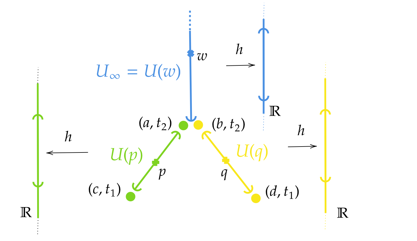
Figure 3: A graphical representation of the display poset, with its a.e. covering - see Section 4.2 - highlighted by the brackets at the extremes of the edges. Each such covering is the mapped homeomorphically to $\mathbb{R}$ via the height function $h$. Note that $d((a,t_{2}),(b,t_{2}))=0$ and $\{(a,t_{2}),(b,t_{2})\}=CA((c,t_{1}),(d,t_{1}))$. The color scheme is coherent with the one in Figure 1.

See Figure 3 for an example of a display poset with its pseudo metric structure.

Remark 2

6 states that if $\pi_{0}(X_{\operatorname*{\scalerel*{\cdot}{\bigodot}}})$ is a regular abstract merge tree, then via $E_{T}\hookrightarrow D_{\pi_{0}(X_{\operatorname*{\scalerel*{\cdot}{\bigodot}}})}$, we can induce a metric on $(T,h_{T})$. It is not hard to see that this is the shortest path metric on $E_{T}$, with the length of an edge $e=(v,v^{\prime})$ being given by $h_{T}(v^{\prime})-h_{T}(v)$.

Remark 3

Given $\pi_{0}(X_{\operatorname*{\scalerel*{\cdot}{\bigodot}}})$ abstract merge tree, we have that the quotient of $D_{\pi_{0}(X_{\operatorname*{\scalerel*{\cdot}{\bigodot}}})}$ under the relationship $x\sim y$ iff $d(x,y)=0$, is isometric as a metric space to $D_{R(\pi_{0}(X_{\operatorname*{\scalerel*{\cdot}{\bigodot}}}))}$.

4.3 Functions Spaces on the Display Poset

Thanks to 6 any display poset of an abstract merge tree inherits the topology generated by the open balls of the (pseudo) metric.

Consider now an abstract merge tree $\pi_{0}(X_{\operatorname*{\scalerel*{\cdot}{\bigodot}}})$ with critical set $\{t_{1},\ldots,t_{n}\}$ and let $t\neq t_{i}$ for all $i=1,\ldots,n$. Consider $p=(a,t)\in D_{\pi_{0}(X_{\operatorname*{\scalerel*{\cdot}{\bigodot}}})}$. We call $t_{p}=\max\{h(q)\in\{t_{1},\ldots,t_{n}\}\text{ with }q<p\}$ and $t^{p}=\min\{h(q)\in\{t_{1},\ldots,t_{n}\}\text{ with }q>p\}$. An open ball of radius $\varepsilon>0$ is by definition:

$$B_{\varepsilon}(p):=\{q\in D_{\pi_{0}(X_{\operatorname*{\scalerel*{\cdot}{\bigodot}}})}\mid d(p,q)<\varepsilon\}.$$

Consider now $\varepsilon>0$, with $t_{p}\leq t-\varepsilon<t+\varepsilon\leq t^{p}$. Let $p=(a,t)$ be a point such that for every $\eta>0$ small enough $\#X_{t-\eta<t}^{-1}(p)=1$ and $\#X_{t<t+\eta}^{-1}(X_{t<t+\eta}(p))=1$. The ball of radius $\varepsilon$ around $p$ is:

$$B_{\varepsilon}(p):=\{q\in\operatorname*{CA}(\{p\})\mid h(q)<t+\varepsilon\}\bigcup\{q\mid p\in\operatorname*{CA}(\{q\})\text{ and }h(q)>t-\varepsilon\}.$$

Thus, for any such point $p=(a,t)$ we can define the set:

$$U(p):=\{q\in\operatorname*{CA}(\{p\})\mid h(q)<t^{p}\}\bigcup\{q\mid p\in\operatorname*{CA}(\{q\})\text{ and }h(q)>t_{p}\}$$

which is an open neighbor of $p$. If $t>t_{n}$, then $t^{p}=\infty$ and so we have:

$$U_{\infty}:=U(p)=\{q\in\operatorname*{CA}(\{(\star,t_{n})\})\mid h(q)>t_{n}\}.$$

Refer to Figure 3 to have a visual intuition for the following proposition.

Proposition 7

The map $h:D_{\pi_{0}(X_{\operatorname*{\scalerel*{\cdot}{\bigodot}}})}\rightarrow\mathbb{R}$ is monotone, continuous and $h_{\mid U(p)}:U(p)\rightarrow(t_{p},t^{p})$ is an homeomorphism and an isometry.

Proof  Using the same notation of 6, we have:

$$\mid h((a,t))-h((b,t\textasciiacute))\mid=\mid t-t^{\prime}\mid\leq\tilde{t}-t+\tilde{t}-t^{\prime}=d((a,t),(b,t^{\prime})).$$

Thus $h$ is continuous. Monotonicity is trivial. Suppose now we have $p=(a,t)$ and $(b,t^{\prime}),(c,t^{\prime\prime})\in U(p)$ such that $t^{\prime}=t^{\prime\prime}$ and $b\neq c$. This is absurd since it implies that either $\#X_{t-\varepsilon<t}^{-1}(p)>1$ or $X_{t<t+\varepsilon}^{-1}(X_{t<t+\varepsilon}(p))>1$ depending on whether $t>t^{\prime}$ or $t<t^{\prime}$, respectively. Moreover $h_{\mid U(p)}$ is clearly surjective for $h(X_{t<t^{\prime}}(p))=t^{\prime}$. Thus $h_{\mid U(p)}$ is a bijective map. If $(b,t^{\prime}),(c,t^{\prime\prime})\in U(p)$, $\tilde{t}=\inf\{h(q)\mid q\in\operatorname*{CA}(\{(b,t^{\prime}),(c,t^{\prime\prime})\})\}=\min\{t^{\prime},t^{\prime\prime}\}$, which implies that $h_{\mid U(p)}$ is an isometry. And thus an homeomorphism.  

Definition 17

The set $\mathcal{U}(D_{\pi_{0}(X_{\operatorname*{\scalerel*{\cdot}{\bigodot}}})}):=\{U\subset D_{\pi_{0}(X_{\operatorname*{\scalerel*{\cdot}{\bigodot}}})}\mid U=U(p)\text{ for some }p\in D_{\pi_{0}(X_{\operatorname*{\scalerel*{\cdot}{\bigodot}}})}\}$ is called the a.e. canonical covering of $D_{\pi_{0}(X_{\operatorname*{\scalerel*{\cdot}{\bigodot}}})}$.

Remark 4

Recall that the sets $U(p)$ are defined only for points $p=(a,t)$ for which there is $K>0$ such that for every $0<\varepsilon<K$, we have $\#X_{t-\varepsilon<t}^{-1}(p)=1$ and $\#X_{t<t+\varepsilon}^{-1}(X_{t<t+\varepsilon}(p))=1$.

Note that $\mathcal{U}(D_{\pi_{0}(X_{\operatorname*{\scalerel*{\cdot}{\bigodot}}})})$ is finite by the finiteness of $\pi_{0}(X_{\operatorname*{\scalerel*{\cdot}{\bigodot}}})$. Moreover, if $U(p),U(q)\in\mathcal{U}(D_{\pi_{0}(X_{\operatorname*{\scalerel*{\cdot}{\bigodot}}})})$ then either $U(p)=U(q)$ or $U(p)\bigcap U(q)=\emptyset$.

In fact, for every $t,t^{\prime}\in h(U)$, $U\in\mathcal{U}(D_{\pi_{0}(X_{\operatorname*{\scalerel*{\cdot}{\bigodot}}})})$, the map $\pi_{0}(X_{t\leq t^{\prime}})$ is injective on $U\cap X_{t}$ and $U\cap X_{t^{\prime}}$. But having $(c,t^{\prime})\in U(p)\bigcap U(q)$ implies $\pi_{0}(X_{t\leq t^{\prime}})(a)=\pi_{0}(X_{t\leq t^{\prime}})(b)=(c,t^{\prime})$ for some $(a,t)\in U(p)$ and $(b,t)\in U(q)$. But then $t^{\prime}\geq t_{p},t_{q}$, which is absurd.

With the help of $\mathcal{U}(D_{\pi_{0}(X_{\operatorname*{\scalerel*{\cdot}{\bigodot}}})})$ we want to induce a measure on the sigma algebra generated by the open sets of $D_{\pi_{0}(X_{\operatorname*{\scalerel*{\cdot}{\bigodot}}})}$. For a display poset $D_{\pi_{0}(X_{\operatorname*{\scalerel*{\cdot}{\bigodot}}})}$ we define the measure $\mu_{\pi_{0}(X_{\operatorname*{\scalerel*{\cdot}{\bigodot}}})}$ as:

$$\mu_{\pi_{0}(X_{\operatorname*{\scalerel*{\cdot}{\bigodot}}})}(Q)=\sum_{U\in\mathcal{U}(D_{\pi_{0}(X_{\operatorname*{\scalerel*{\cdot}{\bigodot}}})})}\mathcal{L}(h(U\bigcap Q))$$

A graphical representation of such measure can be found in Figure 4(a). Note that, if we call $D_{\pi_{0}(X_{\operatorname*{\scalerel*{\cdot}{\bigodot}}})}^{\circ}=\bigcup_{U\in\mathcal{U}(D_{\pi_{0}(X_{\operatorname*{\scalerel*{\cdot}{\bigodot}}})})}U$, we have $\mu_{\pi_{0}(X_{\operatorname*{\scalerel*{\cdot}{\bigodot}}})}(D_{\pi_{0}(X_{\operatorname*{\scalerel*{\cdot}{\bigodot}}})}-D_{\pi_{0}(X_{\operatorname*{\scalerel*{\cdot}{\bigodot}}})}^{\circ})=0$.

Proposition 8

$\mu_{\pi_{0}(X_{\operatorname*{\scalerel*{\cdot}{\bigodot}}})}(Q)=\sum_{U\in\mathcal{U}(D_{\pi_{0}(X_{\operatorname*{\scalerel*{\cdot}{\bigodot}}})})}\mathcal{L}(h(U\bigcap Q))$ induces a measure on the sigma algebra generated by the open sets of $D_{\pi_{0}(X_{\operatorname*{\scalerel*{\cdot}{\bigodot}}})}$.

Proof 

We prove that $\mu_{\pi_{0}(X_{\operatorname*{\scalerel*{\cdot}{\bigodot}}})}$ is $\sigma$-additive. Let $X_{i}$, $i\in\mathbb{N}$, be disjoint sets in the Borel sigma algebra of $D_{\pi_{0}(X_{\operatorname*{\scalerel*{\cdot}{\bigodot}}})}$; we need to prove that $\mu_{\pi_{0}(X_{\operatorname*{\scalerel*{\cdot}{\bigodot}}})}(\bigcup_{i\in\mathbb{N}}X_{i})=\sum_{i\in\mathbb{N}}\mu_{\pi_{0}(X_{\operatorname*{\scalerel*{\cdot}{\bigodot}}})}(X_{i})$.

We have:

$$(\bigcup_{i\in\mathbb{N}}X_{i})\bigcap U=\{p\in D_{\pi_{0}(X_{\operatorname*{\scalerel*{\cdot}{\bigodot}}})}\mid p\in X_{i}\text{ for some }i\text{ and }p\in U\}=\bigcup_{i\in\mathbb{N}}(X_{i}\bigcap U)$$

and so we are finished since $\mathcal{L}$ is $\sigma$-additive on $h(U\bigcap X_{i})$. Note that, if $Q$ is in the Borel sigma algebra of $D_{\pi_{0}(X_{\operatorname*{\scalerel*{\cdot}{\bigodot}}})}$, being $h$ an homeomorphism on $U$ (due to 7), $h(U\bigcap Q)$ is always Lebesgue measurable in $\mathbb{R}$.

 

In a similar fashion, consider a function $f:D_{\pi_{0}(X_{\operatorname*{\scalerel*{\cdot}{\bigodot}}})}\rightarrow\mathbb{R}$: by construction we have that $f$ is $\mu_{\pi_{0}(X_{\operatorname*{\scalerel*{\cdot}{\bigodot}}})}$-measurable if $f\circ(h_{\mid U})^{-1}$ is $\mathcal{L}$-measurable on $\mathbb{R}$ for every $U\in\mathcal{U}(D_{\pi_{0}(X_{\operatorname*{\scalerel*{\cdot}{\bigodot}}})})$. So, given a $\mu_{\pi_{0}(X_{\operatorname*{\scalerel*{\cdot}{\bigodot}}})}$-measurable function $f:D_{\pi_{0}(X_{\operatorname*{\scalerel*{\cdot}{\bigodot}}})}\rightarrow\mathbb{R}$ we can define:

$$\int_{D_{\pi_{0}(X_{\operatorname*{\scalerel*{\cdot}{\bigodot}}})}}fd\mu_{\pi_{0}(X_{\operatorname*{\scalerel*{\cdot}{\bigodot}}})}=\sum_{U(p)\in\mathcal{U}(D_{\pi_{0}(X_{\operatorname*{\scalerel*{\cdot}{\bigodot}}})})}\int_{t_{p}}^{t^{p}}f\circ(h_{\mid U(p)})^{-1}d\mathcal{L}.$$

Leveraging on this definition, we want to define a framework to work with functions defined in some metric space $(E,d_{e})$. For reasons which will be clarified in the next section, we want that inside the metric space $E$ there is a reference element $0$ such that the amount of information contained in the value $f(p)$ can in some sense be quantified as the distance $d_{e}(f(p),0)$. So we make the following assumption.

Assumption 3

We always assume that $(E,d_{e})$ is a metric space and that $(E,\ast,0)$ is a monoid, i.e. that $\ast$ is an associative operation with neutral element $0$.

We establish the following notation for any measure space $(M,\mu)$:

$$L_{p}(M,E):=\Big{\{}f:M\rightarrow E\mid d(f(\cdot),0):M\rightarrow\mathbb{R}\text{ measurable and }\int_{M}d_{e}(f(\cdot),0)^{p}d\mu<\infty\Big{\}}/\sim$$

with $\sim$ being the usual equivalence relationship between functions identifying functions up to $\mu$-zero measure sets. This space becomes a monoid and a metric space with $(f+g)(p):=f(p)\ast g(p)$ and:

$$d_{L_{p}}(f,g)=\int_{M}d_{e}(f(\cdot),g(\cdot))^{p}d\mu.$$

To verify that $d_{L_{p}}$ is a metric is enough to see that $d_{L_{p}}(f,g)=0$ if and only if $f$ and $g$ differ on $\mu$-zero measure sets and prove the triangle inequality using that $L_{p}(M,\mathbb{R})$ is a normed space.

For the sake of brevity, in the following we do not write explicitly the request that $d(f(\cdot),0)$ is measurable and we imply it in the existence of its integral. Thus, we are interested in the spaces:

$$L_{p}(\pi_{0}(X_{\operatorname*{\scalerel*{\cdot}{\bigodot}}}),E):=\Big{\{}f:D_{\pi_{0}(X_{\operatorname*{\scalerel*{\cdot}{\bigodot}}})}\rightarrow E\mid\int_{D_{\pi_{0}(X_{\operatorname*{\scalerel*{\cdot}{\bigodot}}})}}d_{e}(f(\cdot),0)^{p}d\mu_{\pi_{0}(X_{\operatorname*{\scalerel*{\cdot}{\bigodot}}})}<\infty\Big{\}}/\sim$$

Consider now $\pi_{0}(X_{\operatorname*{\scalerel*{\cdot}{\bigodot}}})$ and $\pi_{0}(Y_{\operatorname*{\scalerel*{\cdot}{\bigodot}}})$ such that $\pi_{0}(X_{\operatorname*{\scalerel*{\cdot}{\bigodot}}})\cong_{a.e.}\pi_{0}(Y_{\operatorname*{\scalerel*{\cdot}{\bigodot}}})$. Let $Z\subset\mathbb{R}$ such that $\alpha:\pi_{0}(X_{\operatorname*{\scalerel*{\cdot}{\bigodot}}\mid Z})\rightarrow\pi_{0}(Y_{\operatorname*{\scalerel*{\cdot}{\bigodot}}\mid Z})$ is a natural isomorphism and $\mathcal{L}(\mathbb{R}-Z)=0$. Then $\alpha$ induces a bijection between the display posets:

$$D_{\pi_{0}(X_{\operatorname*{\scalerel*{\cdot}{\bigodot}}\mid Z})}:=\bigcup_{t\in Z}\pi_{0}(X_{t})\times\{t\}$$

and

$$D_{\pi_{0}(Y_{\operatorname*{\scalerel*{\cdot}{\bigodot}}\mid Z})}:=\bigcup_{t\in Z}\pi_{0}(Y_{t})\times\{t\}.$$

With an abuse of notation we call such bijection $\alpha:D_{\pi_{0}(X_{\operatorname*{\scalerel*{\cdot}{\bigodot}}\mid Z})}\rightarrow D_{\pi_{0}(Y_{\operatorname*{\scalerel*{\cdot}{\bigodot}}\mid Z})}$.

Given $f:D_{\pi_{0}(Y_{\operatorname*{\scalerel*{\cdot}{\bigodot}}})}\rightarrow E$ we can clearly restrict it to $D_{\pi_{0}(Y_{\operatorname*{\scalerel*{\cdot}{\bigodot}}\mid Z})}$ and thus we can pull it back on $D_{\pi_{0}(X_{\operatorname*{\scalerel*{\cdot}{\bigodot}}\mid Z})}$ with $\alpha$:

$$D_{\pi_{0}(X_{\operatorname*{\scalerel*{\cdot}{\bigodot}}\mid Z})}\xrightarrow{\alpha}D_{\pi_{0}(Y_{\operatorname*{\scalerel*{\cdot}{\bigodot}}\mid Z})}\hookrightarrow D_{\pi_{0}(Y_{\operatorname*{\scalerel*{\cdot}{\bigodot}}})}\xrightarrow{f}E$$

We call such function $\alpha^{*}f$.

Proposition 9

The rule $f\mapsto\alpha^{*}f$ described above induces map $\alpha^{*}:L_{p}(D_{\pi_{0}(X_{\operatorname*{\scalerel*{\cdot}{\bigodot}}})},E)\rightarrow L_{p}(D_{\pi_{0}(Y_{\operatorname*{\scalerel*{\cdot}{\bigodot}}})},E)$ which is an isometry and a map of monoids.

Proof  Since $\mathcal{L}(\mathbb{R}-Z)=0$ then both $f\in L_{p}(D_{\pi_{0}(Y_{\operatorname*{\scalerel*{\cdot}{\bigodot}}\mid Z})},E)$ and $\alpha^{*}f\in L_{p}(D_{\pi_{0}(X_{\operatorname*{\scalerel*{\cdot}{\bigodot}}\mid Z})},E)$ identify a unique equivalence class, respectively, in $L_{p}(D_{\pi_{0}(Y_{\operatorname*{\scalerel*{\cdot}{\bigodot}}})},E)$ and $L_{p}(D_{\pi_{0}(X_{\operatorname*{\scalerel*{\cdot}{\bigodot}}})},E)$. Moreover, it is easy to see that the map $\alpha^{*}$ is such that $\alpha^{*}(f+g)=\alpha^{*}f+\alpha^{*}g$ and $d_{L_{p}}(f,g)=d_{L_{p}}(\alpha^{*}f,\alpha^{*}g)$. Lastly, because $\alpha$ is a natural isomorphism, then $(\alpha^{-1})^{*}$ yields the opposite correspondence.  

9 implies that, for our purposes, we can always restrict ourselves to considering regular abstract merge trees. Thus we make the following assumption.

Assumption 4

From now on we will always suppose that any abstract merge tree we consider is regular.

4.4 Local Representations of Functions

When comparing two functions $f$, $g$ defined on different display posets, we face the problem of combining together two kinds of variability: using language borrowed from functional data analysis (see the Special Section on Time Warpings and Phase Variation on the Electronic Journal of Statistics, Vol 8 (2), and references therein) and shape analysis (Kendall, 1977, 1984; Dryden and Mardia, 1998) we have an “horizontal” variability, due to the different domains (i.e. display posets), and a “vertical” variability which depends on the actual values that the functions assume. It is reasonable that both kinds of variability contribute to the final distance value: we have a cost given by the aligning the two display posets - horizontal variability - and a cost arising from the different amplitudes of the functions - vertical variability. In particular, we would like the horizontal variability to be measured in a way which is suitable for abstract merge trees (for instance, it should posses some kind of stability properties) and, similarly, the way in which the amplitude variability is measured should assume a somehow natural form, related to the spaces $L_{p}(D_{\pi_{0}(X_{\operatorname*{\scalerel*{\cdot}{\bigodot}}})},E)$.

In other words, given $f:D_{\pi_{0}(X_{\operatorname*{\scalerel*{\cdot}{\bigodot}}})}\rightarrow E$ and $g:D_{\pi_{0}(Y_{\operatorname*{\scalerel*{\cdot}{\bigodot}}})}\rightarrow E$ we want to align, deform the display posets by locally comparing the information given by $f$ and $g$ and matching the display posets in the more convenient way. The word locally is on purpose vague at this stage of the discussion and should be thought as in some neighborhood of points of the posets. To compare local information carried by functions, we need to embed such objects in a common space so that differences can be measured.

First we formalize the procedure of obtaining local information from a function $f:D_{\pi_{0}(X_{\operatorname*{\scalerel*{\cdot}{\bigodot}}})}\rightarrow E$ - Figure 4(b) can help in the visualization of such idea. Given $D_{\pi_{0}(X_{\operatorname*{\scalerel*{\cdot}{\bigodot}}})}$ display poset and its a.e. canonical covering, we have an isomorphism of metric spaces and monoids:

$$L_{p}(\pi_{0}(X_{\operatorname*{\scalerel*{\cdot}{\bigodot}}}),E)\cong\bigoplus^{p}_{U\in\mathcal{U}(D_{\pi_{0}(X_{\operatorname*{\scalerel*{\cdot}{\bigodot}}})})}L_{p}(h(U),E)$$

where $\bigoplus^{p}$ means that the norm of the direct sum is the $p$-th root of the sum of the $p$-th powers of the elements in the direct sum.

In this way we split up a function $f$ on open disjoint subsets, without losing any information. However, as in Figure 4, to compare different functions one may need to represent this information on a finer scale and thus $\mathcal{U}_{D_{\pi_{0}(X_{\operatorname*{\scalerel*{\cdot}{\bigodot}}})}}$ may not be the correct way to split up $f$, which may need to be partitioned in smaller pieces. Thus we allow $\mathcal{U}_{D_{\pi_{0}(X_{\operatorname*{\scalerel*{\cdot}{\bigodot}}})}}$ to be refined with particular collections of open sets.

Definition 18

A collection of open sets of $D_{\pi_{0}(X_{\operatorname*{\scalerel*{\cdot}{\bigodot}}})}$ is an a.e. covering of $D_{\pi_{0}(X_{\operatorname*{\scalerel*{\cdot}{\bigodot}}})}$ if it covers $D_{\pi_{0}(X_{\operatorname*{\scalerel*{\cdot}{\bigodot}}})}$ up to $\mu_{\pi_{0}(X_{\operatorname*{\scalerel*{\cdot}{\bigodot}}})}$-zero measure set. An a.e. covering of $D_{\pi_{0}(X_{\operatorname*{\scalerel*{\cdot}{\bigodot}}})}$ is regular if it is made by disjoint, path-connected open sets, each contained in some $U\in\mathcal{U}(D_{\pi_{0}(X_{\operatorname*{\scalerel*{\cdot}{\bigodot}}})})$.

Given $\mathcal{O}^{\prime}$ regular a.e. covering of $D_{\pi_{0}(X_{\operatorname*{\scalerel*{\cdot}{\bigodot}}})}$, a refinement of $\mathcal{O}^{\prime}$ is a regular a.e. covering $\mathcal{O}$ such that for every $U\in\mathcal{O}$ there is $U^{\prime}\in\mathcal{O}^{\prime}$ such that $U\subset U^{\prime}$.

Given the display poset $D_{\pi_{0}(X_{\operatorname*{\scalerel*{\cdot}{\bigodot}}})}$ of an abstract merge tree $\pi_{0}(X_{\operatorname*{\scalerel*{\cdot}{\bigodot}}})$ we collect all the refinements of its a.e. canonical covering in the set $\operatorname*{Cov}(\pi_{0}(X_{\operatorname*{\scalerel*{\cdot}{\bigodot}}}))$.

Proposition 10

The set $\operatorname*{Cov}(\pi_{0}(X_{\operatorname*{\scalerel*{\cdot}{\bigodot}}}))$ is a lattice. It is a poset with the relationship $\mathcal{O}<\mathcal{O}^{\prime}$ if $\mathcal{O}$ is a refinement of $\mathcal{O}^{\prime}$ and for every couple of elements $\mathcal{O}$, $\mathcal{O}^{\prime}$ there is a unique least upper bound $\mathcal{O}\vee\mathcal{O}^{\prime}$ and a unique greater lower bound $\mathcal{O}\wedge\mathcal{O}^{\prime}$. The operations are defined as follows:

$$\mathcal{O}\vee\mathcal{O}^{\prime}:=\pi_{0}\left(\bigcup_{U\in\mathcal{O}^{\prime}\text{ or }U\in\mathcal{O}}U\right)$$

$$\mathcal{O}\wedge\mathcal{O}^{\prime}:=\{U\cap U^{\prime}\mid U^{\prime}\in\mathcal{O}^{\prime}\text{ and }U\in\mathcal{O}\}.$$

Given $\mathcal{O}\in\operatorname*{Cov}(\pi_{0}(X_{\operatorname*{\scalerel*{\cdot}{\bigodot}}}))$ we have:

$$L_{p}(\pi_{0}(X_{\operatorname*{\scalerel*{\cdot}{\bigodot}}}),E)\cong\bigoplus^{p}_{U\in\mathcal{O}}L_{p}(h(U),E)$$

As already mentioned, to compare functions defined on different abstract merge trees we want to embed all these representations of functions into one common metric space, shared by all abstract merge trees. What we do is to consider $L_{p}((a,b),E)$, for some $(a,b)\subset\mathbb{R}$ and embed it into $L_{p}(\mathbb{R},E)$ by extending $f:(a,b)\rightarrow E$ to $\mathbb{R}$ with $0\in E$ outside $(a,b)$. In this way we have an isometric embedding $L_{p}((a,b),E)\hookrightarrow L_{p}(\mathbb{R},E)$.

In the next definition we need the notion of the essential support of a function $f:(M,\mu)\rightarrow E$ defined on a measure topological space $(M,\mu)$ and with values in $(E,\ast,0)$:

$$\operatorname*{supp}(f)=M-\bigcup\{U\subset M\text{ open }\mid f_{\mid U}=0\text{ }\mu-\text{a.e.}\}$$

Definition 19

Given $D_{\pi_{0}(X_{\operatorname*{\scalerel*{\cdot}{\bigodot}}})}$ and $\mathcal{O}\in\operatorname*{Cov}(\pi_{0}(X_{\operatorname*{\scalerel*{\cdot}{\bigodot}}}))$, a local representation of a function in $L_{p}(D_{\pi_{0}(X_{\operatorname*{\scalerel*{\cdot}{\bigodot}}})},E)$ on $\mathcal{O}$ is a function $\varphi_{\mathcal{O}}:\mathcal{O}\rightarrow L_{p}(\mathbb{R},E)$ such that $\operatorname*{supp}(\varphi_{\mathcal{O}}(U))\subset h(U)$ for every $U\in\mathcal{O}$.

Note that if, instead of splitting $f$ on a finer scale, we want to look at the function on a coarser level, we can do that. Consider $\mathcal{O}^{\prime}$ refinement of $\mathcal{O}$; then for every $V\in\mathcal{O}$:

$$\varphi_{\mathcal{O}}(V)=\sum_{U\in\mathcal{O}^{\prime}\text{ such that }U\subset V}\varphi_{\mathcal{O}^{\prime}}(U)$$

4.5 Regular Coverings and Merge Trees Up to Order $2$ Vertices

Thanks to 9 we have seen that to work with functions defined on display posets we can reduce to the case of regular abstract merge trees. This makes the upcoming discussion much easier since, thanks to 4, we can associate a merge tree to any regular abstract merge tree. In particular, in this section we deal with the problem of associating functional weights to the edges of a merge tree, so that this becomes a combinatorial representation of a function defined on a display poset.

We have already seen that the metric $d$ defined on the display poset $D_{\pi_{0}(X_{\operatorname*{\scalerel*{\cdot}{\bigodot}}})}$ induces the shortest path metric on the graph $(T,h_{T})=\mathcal{M}(\pi_{0}(X_{\operatorname*{\scalerel*{\cdot}{\bigodot}}}))$ via the inclusion $E_{T}\hookrightarrow D_{\pi_{0}(X_{\operatorname*{\scalerel*{\cdot}{\bigodot}}})}$ - see 4. Similarly, we can establish a correspondence between the edges $E_{T}$ and the a.e. canonical covering $\mathcal{U}(D_{\pi_{0}(X_{\operatorname*{\scalerel*{\cdot}{\bigodot}}})})$: each edge $(v,v^{\prime})\in E_{T}$ corresponds to the open set $U=\{p\in D_{\pi_{0}(X_{\operatorname*{\scalerel*{\cdot}{\bigodot}}})}\mid v<p<v^{\prime}\}$ or $U_{\infty}=\{p\in D_{\pi_{0}(X_{\operatorname*{\scalerel*{\cdot}{\bigodot}}})}\mid v<p\}$ if $v^{\prime}=r_{T}$ - as in Figure 2(c). This correspondence can be extended to a bijection between the equivalence class of merge trees up to order $2$ vertices.

Proposition 11

Consider $T=\mathcal{M}(\pi_{0}(X_{\operatorname*{\scalerel*{\cdot}{\bigodot}}}))$ and call $[T]$ the equivalence class of $T$ up to order $2$ vertices. Then $[T]$ and the set $\operatorname*{Cov}(\pi_{0}(X_{\operatorname*{\scalerel*{\cdot}{\bigodot}}}))$ are in bijection, with $T$, the only merge tree in $[T]$ without order $2$ vertices, being mapped to the a.e. canonical covering $\mathcal{U}(D_{\pi_{0}(X_{\operatorname*{\scalerel*{\cdot}{\bigodot}}})})$. Moreover $\mathcal{O}<\mathcal{O^{\prime}}$ if and only if $T_{\mathcal{O}}$ can be obtained from $T_{\mathcal{O^{\prime}}}$ via ghostings.

Proof  The map is induced by each edge $(v,v^{\prime})\in E_{T}$ being sent into the open set $U=\{p\in D_{\pi_{0}(X_{\operatorname*{\scalerel*{\cdot}{\bigodot}}})}\mid v<p<v^{\prime}\}$ or $U_{\infty}=\{p\in D_{\pi_{0}(X_{\operatorname*{\scalerel*{\cdot}{\bigodot}}})}\mid v<p\}$ if $v^{\prime}=r_{T}$. The result then follows from 7 plus the fact that path-connected subsets of $\mathbb{R}$ are connected intervals.  

As a consequence, a local representation of a function on $\mathcal{U}(D_{\pi_{0}(X_{\operatorname*{\scalerel*{\cdot}{\bigodot}}})})$, i.e. $\varphi_{\mathcal{U}(D_{\pi_{0}(X_{\operatorname*{\scalerel*{\cdot}{\bigodot}}})})}:\mathcal{U}(D_{\pi_{0}(X_{\operatorname*{\scalerel*{\cdot}{\bigodot}}})})\rightarrow L_{p}(\mathbb{R},E)$ induces a unique function $\varphi_{T}:E_{T}\rightarrow L_{p}(\mathbb{R},E)$, and viceversa. Moreover, consider $\mathcal{M}(\pi_{0}(X_{\operatorname*{\scalerel*{\cdot}{\bigodot}}}))=(T,h_{T})$ and $(T^{\prime},h_{T^{\prime}})$ such that $T^{\prime}$ and $T$ are equivalent up to order two vertices. We know that $\pi_{0}(X_{\operatorname*{\scalerel*{\cdot}{\bigodot}}})=\mathcal{F}((T^{\prime},h_{T^{\prime}}))\cong\mathcal{F}((T,h_{T}))$. By 11, $V_{T}\hookrightarrow D_{\pi_{0}(X_{\operatorname*{\scalerel*{\cdot}{\bigodot}}})}$ induces the a.e. canonical covering $\mathcal{U}(D_{\pi_{0}(X_{\operatorname*{\scalerel*{\cdot}{\bigodot}}})})$ and the inclusion $V_{T^{\prime}}\hookrightarrow D_{\pi_{0}(X_{\operatorname*{\scalerel*{\cdot}{\bigodot}}})}$ induces another regular a.e. covering, which is a refinement of $\mathcal{U}(D_{\pi_{0}(X_{\operatorname*{\scalerel*{\cdot}{\bigodot}}})})$, giving two different local representations of the same function. Thus, we immediately obtain the following corollary, finally bridging between functions defined on display posets and weighted trees.

Corollary 2

Given an abstract merge tree $\pi_{0}(X_{\operatorname*{\scalerel*{\cdot}{\bigodot}}})$ and the merge tree $T=\mathcal{M}(\pi_{0}(X_{\operatorname*{\scalerel*{\cdot}{\bigodot}}}))$, we have a bijection between the following sets:

$$\{\varphi_{\mathcal{O}}:\mathcal{O}\rightarrow L_{p}(\mathbb{R},E)\mid\mathcal{O}\in\operatorname*{Cov}(\pi_{0}(X_{\operatorname*{\scalerel*{\cdot}{\bigodot}}}))\text{ and }\operatorname*{supp}(\varphi_{\mathcal{O}}(U))\subset h(U),\forall U\in\mathcal{O}\}$$

and

$$\{\varphi_{T^{\prime}}:E_{T^{\prime}}\rightarrow L_{p}(\mathbb{R},E)\mid T^{\prime}\in[T]\text{ and }\operatorname*{supp}(\varphi_{T^{\prime}}((v,v^{\prime})))\subset[h_{T^{\prime}}(v),h_{T^{\prime}}(v^{\prime})],\forall(v,v^{\prime})\in E_{T^{\prime}}\}.$$

To sum up, we have proven that the local representation of a function on the display poset of an abstract merge tree is equivalent to a weighted tree, equal up to order $2$ vertices to the merge tree representing the regular abstract merge tree, with the weights being the restriction of the original function to a suitable interval. For notational convenience, from now on, we may confuse the two sets in 2, calling local representation of function also $\varphi_{T^{\prime}}:E_{T^{\prime}}\rightarrow L_{p}(\mathbb{R},E)$ satisfying the requested properties.

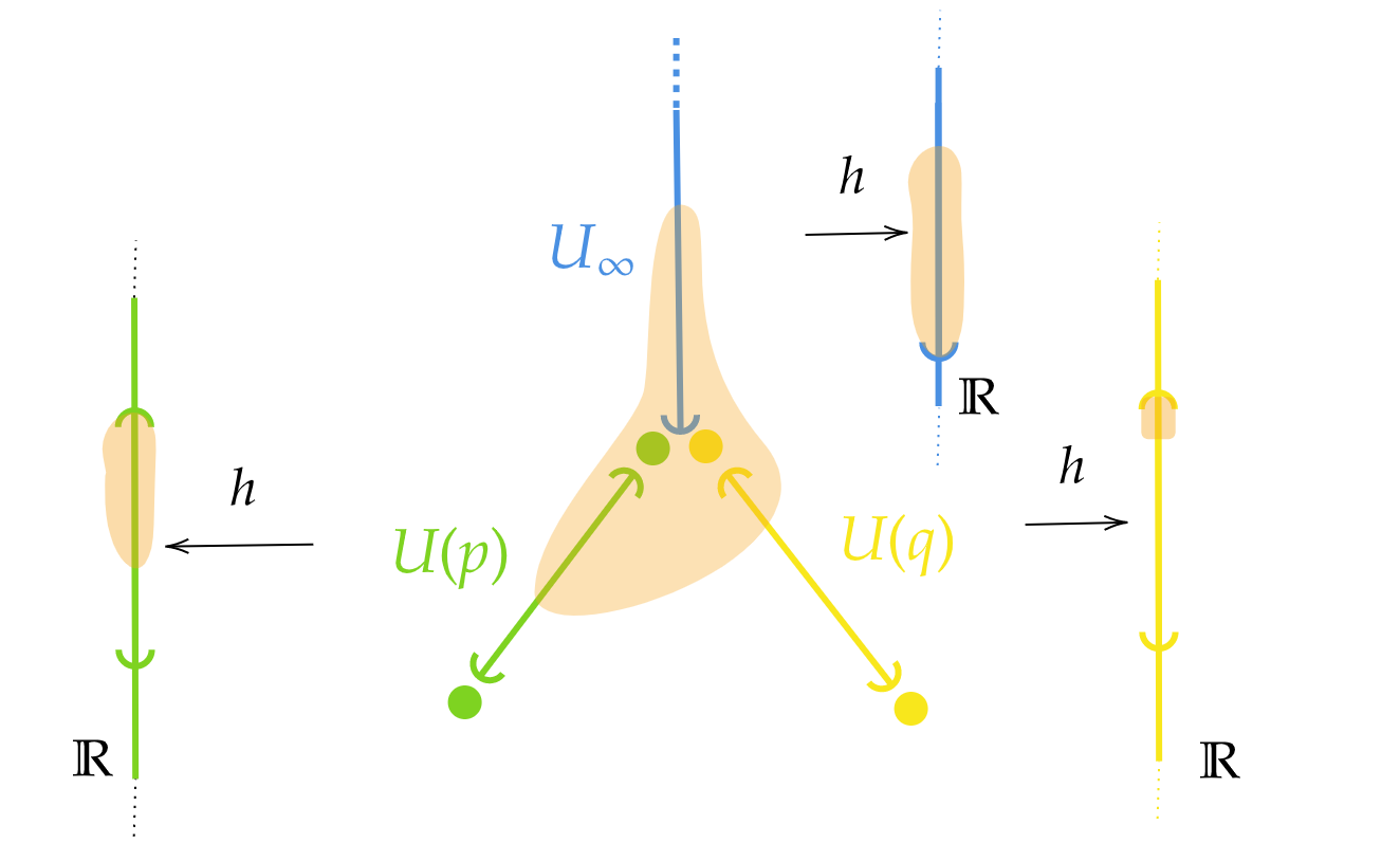
(a) A display poset $D_{\pi_{0}(X_{\operatorname*{\scalerel*{\cdot}{\bigodot}}})}$ with the measure $\mu_{D_{\pi_{0}(X_{\operatorname*{\scalerel*{\cdot}{\bigodot}}})}}$. The orange shaded set is first intersected with the open sets $U_{\infty}$, $U(p)$ and $U(q)$ and then its Lebesgue measure is taken in $\mathbb{R}$ via the height function $h$.

(b) A function $f:D_{\pi_{0}(X_{\operatorname*{\scalerel*{\cdot}{\bigodot}}})}\rightarrow\mathbb{R}$ defined on the display poset $D_{\pi_{0}(X_{\operatorname*{\scalerel*{\cdot}{\bigodot}}})}$. With different colors we have highlighted the restrictions of the function on the different open sets of the canonical a.e. covering.

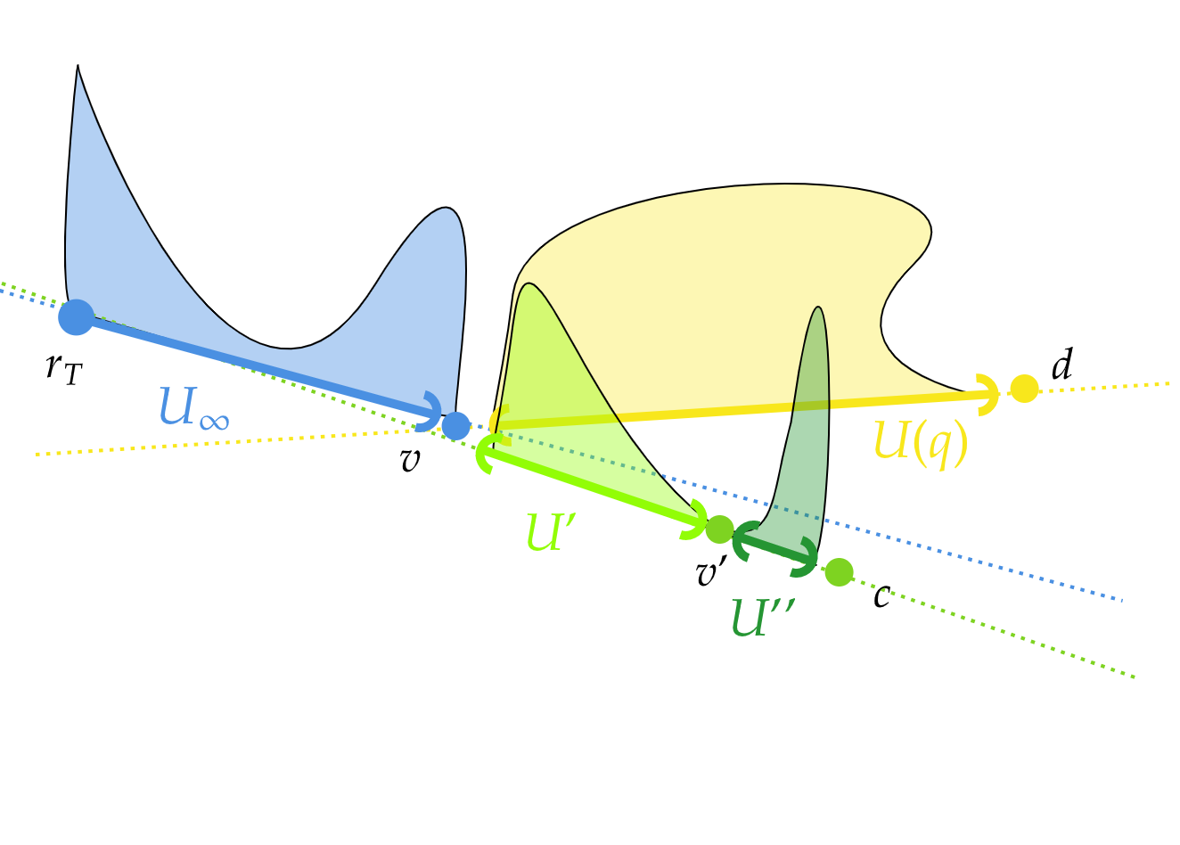
(c) A function $f:D_{\pi_{0}(X_{\operatorname*{\scalerel*{\cdot}{\bigodot}}})}\rightarrow\mathbb{R}$ defined on the display poset $D_{\pi_{0}(X_{\operatorname*{\scalerel*{\cdot}{\bigodot}}})}$ represented with the restrictions on a regular a.e. covering which refines the canonical one.

(d) A function $g:D_{\pi_{0}(Y_{\operatorname*{\scalerel*{\cdot}{\bigodot}}})}\rightarrow\mathbb{R}$ defined on the display poset $D_{\pi_{0}(Y_{\operatorname*{\scalerel*{\cdot}{\bigodot}}})}$ along with its restrictions on the canonical a.e. covering of $D_{\pi_{0}(Y_{\operatorname*{\scalerel*{\cdot}{\bigodot}}})}$. The refinement of the canonical a.e. covering of $D_{\pi_{0}(X_{\operatorname*{\scalerel*{\cdot}{\bigodot}}})}$ which appears in Figure 4(c) is much more suited than the canonical a.e. covering in Figure 4(b) to compare the two functions: on $U_{\infty}$ and $U_{\infty}$ the functions are very similar, as the are on $U^{\prime}$ and $U(x)$, on $U^{\prime\prime}$ and $U(y)$ and on $U(q)$ and $U(z)$.

Figure 4: Measures and real valued functions defined on display posets. In every plot but the upper left one, for visualization purposes the posets are represented as embedded on the horizontal plane in $\mathbb{R}^{3}$ and plotted with thick lines. The vertical axis represents the value of the functions. With different colors we have highlighted the restrictions of the functions on different open sets. The colored dotted lines are are a qualitative visual representation of the embedding $\left(f:(a,b)\rightarrow\mathbb{R}\right)\mapsto\left(f^{\prime}:\mathbb{R}\rightarrow\mathbb{R}\right)$ where $f^{\prime}$ extends $f$ with $0$ outside $(a,b)$.

5 Edit Distance Between Local Representation of Functions

At this point we face the problem of defining a suitable (pseudo) metric framework for objects of the form $f\in L_{1}(D_{\pi_{0}(X_{\operatorname*{\scalerel*{\cdot}{\bigodot}}})},E)$ and $g\in L_{1}(D_{\pi_{0}(Y_{\operatorname*{\scalerel*{\cdot}{\bigodot}}})},E)$. Each of such objects can be represented by $(T,h_{T},\varphi_{T})$, with $\varphi_{T}:E_{T}\rightarrow L_{p}(\mathbb{R},E)$ such that $\operatorname*{supp}(\varphi_{T}(e))\subset[h_{T}(a),h_{T}(b)]$ for $e=(a,b)$. Thus, we introduce a metric to compare weighted trees relying on the results in Pegoraro (2023), where the weights are given by functions. Then, we also investigate some stability properties of this metric.

5.1 Editing Local Representation of Functions

In Pegoraro (2023) the author defines a distance for objects of the form $(G,\varphi_{G}:E_{G}\rightarrow W)$ - where $G$ is a general (possibly directed) graph, which is inspired by the graph and tree edit distances (Tai, 1979; Gao et al., 2010), but with key differences in the edit operations. The philosophy of edit distances is to allow certain modifications of the base object, called edits, each being associated to a cost, and to define the distance between two objects as the minimal cost that is needed to transform the first object into the second with a finite sequence of edits. In this way, up to properly setting up a set of edits, one can formalize the deformation of a tree comparing the local information induced by the weights of the trees, i.e. the restriction on the edges of a function defined on the display poset.

The framework developed in Pegoraro (2023) requires that codomain of $\varphi_{T}:E_{T}\rightarrow W$ must satisfy certain properties.

Definition 20

A set $W$ is called editable if the following conditions are satisfied:

• $(W,d)$ is a metric space

• $(W,\ast,0)$ is a monoid (that is $W$ has an associative operation $\ast$ with zero element $0$)

• the map $d(0,\cdot):W\rightarrow\mathbb{R}$ is a map of monoids between $(W,\ast)$ and $(\mathbb{R},+)$: $d(0,x\ast y)=d(0,x)+d(0,y)$.

• $d$ is $\ast$ invariant, that is: $d(x,y)=d(z\ast x,z\ast y)=d(x\ast z,y\ast z)$

In Pegoraro (2023) it is shown that if $E$ is an editable space, then also $W=L_{1}(\mathbb{R},E)$ is an editable space. So local representations of functions defined on a display poset fit into this framework as long as $f:D_{\pi_{0}(X_{\operatorname*{\scalerel*{\cdot}{\bigodot}}})}\rightarrow E$ has value in an editable space. Moreover all the sets $\mathbb{R}_{\geq 0}$, $\mathbb{N}_{\geq 0}$ and their finite sums are editable spaces.

There are however situations which we want to avoid because they represent “degenerate” functions which introduce formal complications.

Definition 21

Given an editable space $E$ and a tree-structure $T$, a weight function $\varphi_{T}:E_{T}\rightarrow L_{1}(\mathbb{R},E)$ is proper if we have $0\in\varphi(E_{T})$ if and only if $E_{T}=\emptyset$ and $V_{T}=\{\star\}$. Analogously to Pegoraro (2023), for the sake of brevity we call dendrogram the datum of a merge tree with a proper weight function $\varphi_{T}:E_{T}\rightarrow L_{1}(\mathbb{R},E)$.

Definition 22

Given an (editable) space $L_{1}(\mathbb{R},E)$ the dendrogram space $(\mathcal{T},L_{1}(\mathbb{R},E))$ is given by the set of dendrograms $(T,\varphi_{T})$ with $\varphi_{T}:E_{T}\rightarrow W$ being a proper weight function.

Remark 5

Note that not all dendrograms in $(\mathcal{T},L_{1}(\mathbb{R},E))$ are local representation of functions. In fact, in general, we do not have: $\operatorname*{supp}(\varphi_{T}((v,v^{\prime})))\subset[h_{T}(v),h_{T^{\prime}}(v)],\forall(v,v^{\prime})\in E_{T}$.

Given an editable dendrogram space $(\mathcal{T},L_{1}(\mathbb{R},E))$, we can define our edits.

• We call shrinking of an edge a change of the local representation of a function associated to the edge. The new local representation function must be equal to the previous one on all edges, apart from the “shrunk” one. In other words, for an edge $e$, this means changing the value $\varphi(e)$ with another non zero function in $L_{1}(\mathbb{R},E)$. Note that, in general, shrinkings do not preserve local representations of functions.

• A deletion is an edit with which an edge is deleted from the dendrogram. Consider an edge $(v_{1},v_{2})$. The result of deleting $v_{1}$ is a new tree structure, with the same vertices and edges a part from $v_{1}$ (the smaller one) and $(v_{1},v_{2})$, and with the father of the deleted vertex which gains all of its children. Note that, if we start from a local representation of a function, the result of a deletion is always a local representation of a function. The inverse of the deletion is the insertion of an edge along with its lower vertex. We can insert an edge at a vertex $v$ specifying the name of the new child of $v$, the children of the newly added vertex (that can be either none, or any portion of the children of $v$), and the value of the function on the new edge. Again, insertions do not preserve local representations of functions.

• Lastly, we generalize 11, defining a transformation which eliminates an order two vertex in a dendrogram, changing the local representation of a function. Suppose we have two edges $e=(v_{1},v_{2})$ and $e^{\prime}=(v_{2},v_{3})$, with $v_{1}<v_{2}<v_{3}$. And suppose $v_{2}$ is of order two. Then, we can remove $v_{2}$ and merge $e$ and $e^{\prime}$ into a new edge $e^{\prime\prime}=(v_{1},v_{3})$, with $\varphi(e^{\prime\prime}):=\varphi(e)+\varphi(e^{\prime})$. This transformation is called the ghosting of the vertex. Its inverse transformation is called the splitting of an edge. Also splittings do not preserve local representations of functions.

A dendrogram $T$ can be edited to obtain another dendrogram, on which one can apply a new edit to obtain a third dendrogram and so on. One can think of this as composing two edits $e_{0}$, $e_{1}$ which are not defined on the same dendrogram, since the second edit is defined on the already edited dendrogram. This is what we mean by composition of edits. Any finite composition of edits is referred to as an edit path. The notations we use are functional notations, even if the edits are not operators, since an edit is not defined on the whole space of dendrograms but on a single dendrogram. For example $e_{1}\circ e_{0}(T)$ means that $T$ is edited with $e_{0}$, and then $e_{0}(T)$ with $e_{1}$.

Exploiting the definitions we have just given we can add some other details to the correspondence established by 2, studying the relationships between the ghosting defined in 11 and the one in Section 5.1.

Definition 23

Dendrograms are equal up to order $2$ vertices if they become isomorphic after applying a finite number of ghostings or splittings. We write $(T,\varphi_{T})\cong_{2}(T^{\prime},\varphi_{T^{\prime}})$. We call $(\mathcal{T}_{2},L_{1}(\mathbb{R},E))$ the space of equivalence classes of dendrograms in $(\mathcal{T},L_{1}(\mathbb{R},E))$, equal up to order $2$ vertices.

Consider $\mathcal{M}(\pi_{0}(X_{\operatorname*{\scalerel*{\cdot}{\bigodot}}}))=(T,h_{T})$ and a proper weight function $\varphi_{T}$ with values in some editable space $L_{1}(\mathbb{R},E)$. We know that $\varphi_{T}$ is equivalent to a local representation of a function on $\mathcal{U}(D_{\pi_{0}(X_{\operatorname*{\scalerel*{\cdot}{\bigodot}}})})$ which, in turns, amounts to the datum of a function $f$ in $L_{1}(D_{\pi_{0}(X_{\operatorname*{\scalerel*{\cdot}{\bigodot}}})},E)$. By construction $\varphi_{T}(e)=f\circ(h_{\mid U})^{-1}:(t,t^{\prime})\rightarrow E$, with $U\in\mathcal{U}(D_{\pi_{0}(X_{\operatorname*{\scalerel*{\cdot}{\bigodot}}})})$ being associated to the edge $e$ and $h$ being the height function of $D_{\pi_{0}(X_{\operatorname*{\scalerel*{\cdot}{\bigodot}}})}$.

Consider now the merge tree $(T^{\prime},h_{T^{\prime}})$ obtained by splitting the edge $e$ of the merge tree into $e_{1}=(v,v^{\prime\prime})$ and $e_{2}=(v^{\prime\prime},v^{\prime})$, with $h_{T^{\prime}}(v^{\prime\prime})=t^{\prime\prime}$. By 2, $E_{T^{\prime}}\hookrightarrow D_{\pi_{0}(X_{\operatorname*{\scalerel*{\cdot}{\bigodot}}})}$ induces a refinement $\mathcal{O}$ of the canonical a.e. cover of $D_{\pi_{0}(X_{\operatorname*{\scalerel*{\cdot}{\bigodot}}})}$, given by the replacement of the open set $U$ associated to $e$, with the open sets $(h_{\mid U})^{-1}((h_{T}(v),h_{T}(v^{\prime\prime})))$ and $(h_{\mid U})^{-1}((h_{T}(v^{\prime\prime}),h_{T}(v^{\prime})))$. Then, we can take the local representation of $f$ on $\mathcal{O}$, which gives $\varphi_{T^{\prime}}:E_{T^{\prime}}\rightarrow E$ so that $\varphi_{T^{\prime}}(e_{1})=(\varphi_{T}(e))_{\mid[t,t^{\prime\prime}]}$ and $\varphi_{T^{\prime}}(e_{2})=(\varphi_{T}(e))_{\mid[t^{\prime\prime},t^{\prime}]}$. In other words the dendrogram $(T^{\prime},\varphi_{T^{\prime}})$ can be obtained via a splitting of the edge $e$ from the dendrogram $(T,\varphi_{T})$. And viceversa, we can ghost $v^{\prime\prime}$ in $(T^{\prime},\varphi_{T^{\prime}})$ to go back to $(T,\varphi_{T})$.

With sum this up with the following result.

Corollary 3

Consider $T=\mathcal{M}(\pi_{0}(X_{\operatorname*{\scalerel*{\cdot}{\bigodot}}}))$ and $f\in L_{1}(D_{\pi_{0}(X_{\operatorname*{\scalerel*{\cdot}{\bigodot}}})},E)$. Let the dendrogram $(T,\varphi_{T})$, be any local representation of $f$, and call $[(T,\varphi_{T})]$ the equivalence class of $(T,\varphi_{T})$ up to order $2$ vertices, restricted to local representations of functions. Then we have:

$$[(T,\varphi_{T})]\cong\{\varphi_{\mathcal{O}}:\mathcal{O}\rightarrow L_{1}(\mathbb{R},E)\mid\text{ local repr. of f }\}.$$

Thus, the ghosting and splitting edits for local representation of functions represent the combinatorial equivalent of the lattice operations in $\operatorname*{Cov}(\pi_{0}(X_{\operatorname*{\scalerel*{\cdot}{\bigodot}}}))$: with a splitting we are refining the local representation and with the ghosting we are looking at the function on a coarser a.e. covering. However, we recall again that not all splittings preserve local representations of functions.

5.2 Costs of Edit Operations

Now we associate to every edit a cost so that we can measure distances between functions’ deformations in $(\mathcal{T},L_{1}(\mathbb{R},E))$. The costs of the edit operations are defined as follows:

• if, via shrinking, an edge goes from weight $f$ to weight $g$, then the cost of such operation is $d_{L_{1}}(f,g)$;

• for any deletion/insertion of an edge with local function equal to $f$, the cost is equal to $d_{L_{1}}(f,0)$;

• the cost of ghosting operations is $\mid d_{L_{1}}(f+g,0)-d_{L_{1}}(f,0)-d_{L_{1}}(g,0)\mid=0$.

Definition 24

Given two dendrograms $T$ and $T^{\prime}$ in $(\mathcal{T},L_{1}(\mathbb{R},E))$, define:

• $\Gamma(T,T^{\prime})$ as the set of all finite edit paths between $T$ and $T^{\prime}$;

• $cost(\gamma)$ as the sum of the costs of the edits for any $\gamma\in\Gamma(T,T^{\prime})$;

• the dendrogram edit distance as:

  $$d_{E}(T,T^{\prime})=\inf_{\gamma\in\Gamma(T,T^{\prime})}cost(\gamma)$$

Pegoraro (2023) proves the following result which, together with 3 says that $d_{E}$ is a metric for functions defined on display posets.

Theorem 1 (adapted from Pegoraro (2023))

Given $E$ editable space, $((\mathcal{T}_{2},L_{1}(\mathbb{R},E)),d_{E})$ is a metric space.

Putting together 3 and 1 we have thus obtained a metric to compare $f\in L_{1}(D_{\pi_{0}(X_{\operatorname*{\scalerel*{\cdot}{\bigodot}}})},E)$ and $g\in L_{1}(D_{\pi_{0}(Y_{\operatorname*{\scalerel*{\cdot}{\bigodot}}})},E)$.

5.3 Optimal Edit Paths

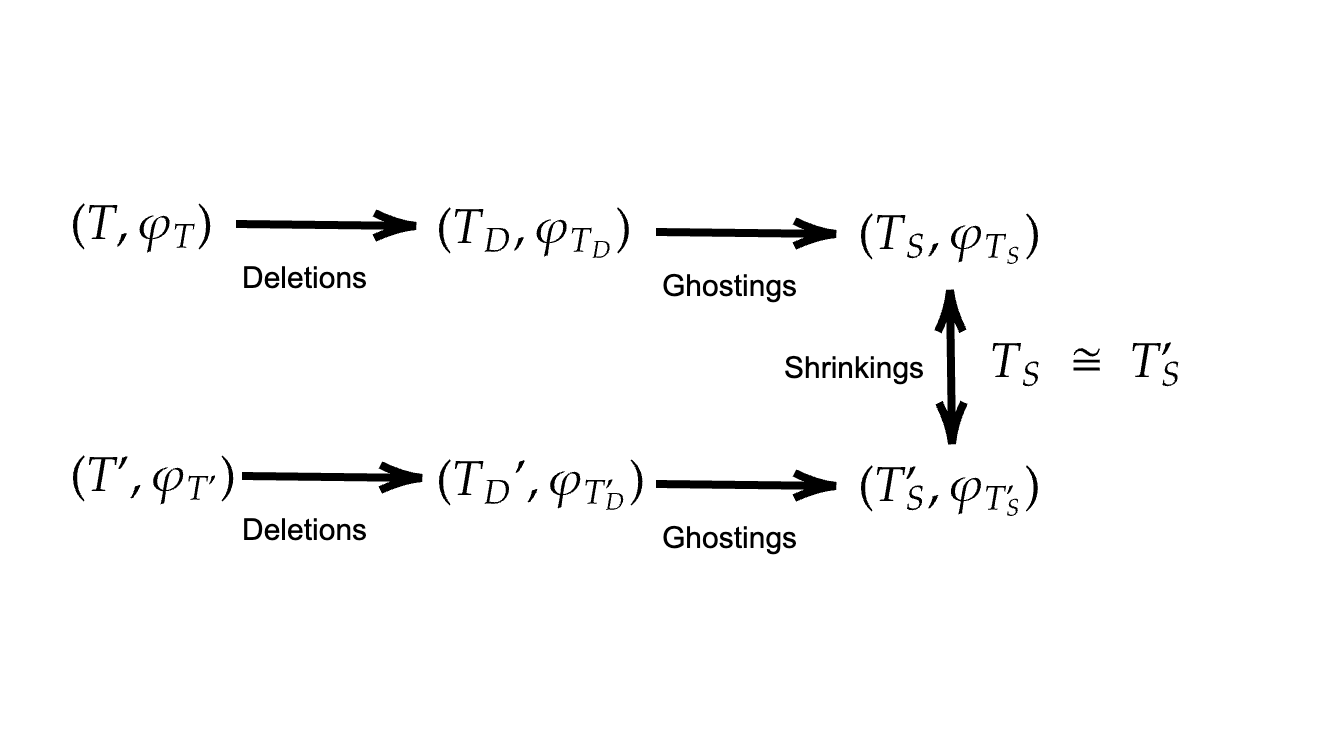
Figure 5: A representation of particular optimal edit paths between dendrograms.

In Section 5.1 we have highlighted that starting from a local representation of $f\in L_{1}(D_{\pi_{0}(X_{\operatorname*{\scalerel*{\cdot}{\bigodot}}})},E)$, after shrinkings, splittings or insertion we in general do not end up with a local representation of a function. While this may be a point which could be improved by future works, we argue that it does not represent a problem in terms of defining a reasonable metric structure to compare $f\in L_{1}(D_{\pi_{0}(X_{\operatorname*{\scalerel*{\cdot}{\bigodot}}})},E)$ and $g\in L_{1}(D_{\pi_{0}(Y_{\operatorname*{\scalerel*{\cdot}{\bigodot}}})},E)$.

In Pegoraro (2023) it is in fact shown that there is always a minimal edit path that operates as in Figure 5. Suppose $(T,\varphi_{T})$ is the starting dendrogram and $(T^{\prime},\varphi_{T^{\prime}})$ the target one: one can operate all deletions on $T$ and then the ghostings on $T$. And do the same on $T^{\prime}$, obtaining respectively the dendrograms $(T_{S},\varphi_{T_{S}})$ and $(T^{\prime}_{S},\varphi_{T._{S}})$. If the starting dendrograms are local representation of functions, then all the dendrograms along these edit paths are still local representation of functions. Thus no metric artefact has appeared up to now.

The properties of such optimal edit paths then imply that the tree structures $T_{S}$ and $T^{\prime}_{S}$ are isomorphic and the shrinkings that take place always turn $\varphi_{T_{S}}(e)$ into $\varphi_{T^{\prime}_{S}}(e^{\prime})$, for some $e\in E_{T_{S}}$ and $e^{\prime}\in E_{T^{\prime}_{S}}$. Thus the shrinking are locally, edge by edge, comparing the functions on $T_{S}$ and $T^{\prime}_{S}$.

5.4 Stability

In this section we establish some stability properties for the metric $d_{E}$ when applied to functions defined on merge trees. To do so, we leverage on the proof of Theorem 1 in Pegoraro and Secchi (2021).

Developing stability results in high generality for functions defined on merge trees is a very broad topic which is outside the aim of the present work. Such results, in fact, require establishing sufficient conditions both for the merge trees to be similar and for the functions to be similar on portions of the merge trees which can be matched together via low-cost mappings. In this context we will deal with the more general of the two issues, removing the problem about similarity of the functions, which is very application-dependent, and focus on how the functional framework we designed is able to handle similarity between merge trees. We will thus consider only a very particular, but meaningful, scenario.

As showcased in the upcoming Section 6, a natural way to produce functions defined on merge trees is to consider a subcategory $\mathcal{B}$ of $\operatorname*{Top}$ and define a function $\Theta:\mathcal{B}\rightarrow E$. Consequently, $f:D_{\pi_{0}(X_{\operatorname*{\scalerel*{\cdot}{\bigodot}}})}\rightarrow E$ can be obtained as $f(a,t)=\Theta(a)$. We call $\varphi^{\Theta}_{T}$ the local representation of such function.

For our purposes we define the constant function $\Theta_{1}:\operatorname*{Top}\rightarrow\mathbb{R}_{\geq 0}$, such that $\Theta_{1}(s)=1$ for all sets $s$. That is $f:D_{\pi_{0}(X_{\operatorname*{\scalerel*{\cdot}{\bigodot}}})}\rightarrow\mathbb{R}_{\geq 0}$ is defined by $f((a,t))=1$. As a consequence we have $f\circ(h_{\mid U(p)})^{-1}=\chi_{(t_{p},t^{p})}$, for some $p\in D_{\pi_{0}(X_{\operatorname*{\scalerel*{\cdot}{\bigodot}}})}$ and with $\chi_{I}$ being the characteristic function over the interval $I\subset\mathbb{R}$. And, if we consider $\mathcal{M}(\pi_{0}(X_{\operatorname*{\scalerel*{\cdot}{\bigodot}}}))=(T,h_{T})$, given $e=(v,v^{\prime})\in E_{T}$, we have $\varphi_{T}(e)=\chi_{(t_{i},t_{j})}=\chi_{(t_{p},t^{p})}$ with $h_{T}(v)=t_{i}$ and $h_{T}(v^{\prime})=t_{j}$. We call $\varphi_{T}^{\Theta_{1}}$ the local representation of the function $f$ induced by $\Theta_{1}$ on $D_{\pi_{0}(X_{\operatorname*{\scalerel*{\cdot}{\bigodot}}})}$. Consider two functions $(T,\varphi^{\Theta_{1}}_{T})$ and $(T^{\prime},\varphi^{\Theta_{1}}_{T^{\prime}})$. Suppose there is $\eta:V_{T}\rightarrow V_{T^{\prime}}$ isomorphism of tree structures such that $\varphi_{T}\circ\eta=\varphi_{T^{\prime}}\circ\eta$. Then $(T,h_{T})\cong(T^{\prime},h_{T^{\prime}})$. In fact via $\eta$, the support of $\varphi_{T}^{\Theta_{1}}(e)$ coincide with the support of $\varphi_{T^{\prime}}^{\Theta_{1}}(\eta(e))$. But the support is given by the critical values of the filtration, that is, the value of the height function $h_{T}$ on the extremes of the edge $e$. So $(T,\varphi^{\Theta_{1}}_{T})\cong(T^{\prime},\varphi^{\Theta_{1}}_{T^{\prime}})$ if and only if $(T,h_{T})\cong(T^{\prime},h_{T^{\prime}})$. Thus, $\Theta_{1}$ gives another way to represent merge trees and so $d_{E}$ between dendrograms of the form $(T,\varphi^{\Theta_{1}}_{T})$ induces a metric between merge trees.

Being the edit distance a summation of the costs of local modification of trees, we expect that the stability properties of $d_{E}$ are quite different from the ones of the bottleneck distance between persistence diagrams, which is defined as the biggest modification ones needs to match two persistence diagrams. Instead, we expect the edit distance to be dependent on the number of vertices in the merge trees but, at the same time, that the cost of the local modifications we need to match the two merge trees goes to $0$. For this reason we give the following definitions.

Definition 25

Given a constructible persistence module $S:\mathbb{R}\rightarrow\operatorname*{Vec}_{\mathbb{K}}$, we define its rank as $\operatorname*{rank}(S):=\#PD(S)$ i.e. the number of points in its persistence diagram. When $S$ is generated on $\mathbb{K}$ by an abstract merge tree $\pi_{0}(X_{\operatorname*{\scalerel*{\cdot}{\bigodot}}})$ we have $\operatorname*{rank}(S):=\#PD(S)=\#L_{T}$, with $(T,h_{T})=\mathcal{M}(\pi_{0}(X_{\operatorname*{\scalerel*{\cdot}{\bigodot}}}))$ and may refer to $\operatorname*{rank}(S)$ also as the rank of the merge tree $\operatorname*{rank}(T)$. We also fix the notation $\dim(T):=\#E_{T}$.

Definition 26

Let $f,g$ be tame functions defined on a path connected topological space $X$. Define $X_{t}=f^{-1}((-\infty,t])$ and $Y_{t}=g^{-1}((-\infty,t])$. Let $T=\mathcal{M}(\pi_{0}(X_{\operatorname*{\scalerel*{\cdot}{\bigodot}}}))$ and $T^{\prime}=\mathcal{M}(\pi_{0}(Y_{\operatorname*{\scalerel*{\cdot}{\bigodot}}}))$ be the merge trees associated to $f$ and $g$ respectively. A metric for merge trees is locally stable if:

$$d(T,T^{\prime})\leq K(\operatorname*{rank}(T)+\operatorname*{rank}(T^{\prime}))\parallel f-g\parallel_{\infty}$$

for some $K>0$.

We want prove that $d_{E}$ induces a locally stable metric on merge trees, via the relationship $(T,h_{T})\cong(T^{\prime},h_{T^{\prime}})$ if and only if $(T,\varphi_{T}^{\Theta_{1}})\cong(T^{\prime},\varphi_{T^{\prime}}^{\Theta_{1}})$.

Corollary 4 (of Theorem 1 in Pegoraro and Secchi (2021))

Let $f,g$ be tame functions defined on a path connected topological space $X$ and such that

$$\text{sup}_{x\in X}|f(x)-g(x)|\leq\varepsilon.$$

Define $X_{t}=f^{-1}((-\infty,t])$ and $Y_{t}=g^{-1}((-\infty,t])$. Let $T=\mathcal{M}(\pi_{0}(X_{\operatorname*{\scalerel*{\cdot}{\bigodot}}}))$ and $T^{\prime}=\mathcal{M}(\pi_{0}(Y_{\operatorname*{\scalerel*{\cdot}{\bigodot}}}))$ be the merge trees associated to $f$ and $g$ respectively.

Then, there exists an edit path $\gamma$ between $V_{T}$ and $V_{T^{\prime}}$ such that:

• $\gamma$ contains at most one edit per edge of $T$ and one per edge of $T^{\prime}$;

• any deletion of an edge $e=(v,v^{\prime})$ is such that $h_{T}(v^{\prime})-h_{T}(v)\leq 2\varepsilon$;

• for any edge $(v,v^{\prime})$ which is shrunk on $(w,w^{\prime})$ after all ghostings and deletions on $T$ and on $T^{\prime}$ we have $\mid h_{T}(v)-h_{T^{\prime}}(w)\mid<\varepsilon$ and $\mid h_{T}(v^{\prime})-h_{T^{\prime}}(w^{\prime})\mid<\varepsilon$ (if $v^{\prime}\neq r_{T}$ and $w^{\prime}\neq r_{T^{\prime}}$).

Leveraging on such result, we can state the following stability result for functions of the form $(T,\varphi_{T}^{\Theta_{1}})$, which implies the local stability of $d_{E}$.

Theorem 2

Let $f,g$ be tame functions defined on a path connected topological space $X$ and such that

$$\text{sup}_{x\in X}|f(x)-g(x)|\leq\varepsilon.$$

Define $X_{t}=f^{-1}((-\infty,t])$ and $Y_{t}=g^{-1}((-\infty,t])$. Lastly, let $T=\mathcal{M}(\pi_{0}(X_{\operatorname*{\scalerel*{\cdot}{\bigodot}}}))$ and $T^{\prime}=\mathcal{M}(\pi_{0}(Y_{\operatorname*{\scalerel*{\cdot}{\bigodot}}}))$ be the merge trees associated to $f$ and $g$ respectively. And let $(T,\varphi_{T}^{\Theta_{1}})$ and $(T^{\prime},\varphi_{T^{\prime}}^{\Theta_{1}})$.

Then, there exists an edit path $\gamma=e_{1}\circ\ldots e_{N}$ between $V_{T}$ and $V_{T^{\prime}}$ such that $cost(e_{i})<2\cdot\varepsilon$, and $N\leq\operatorname*{rank}(T)+\operatorname*{rank}(T^{\prime})$.

6 Examples

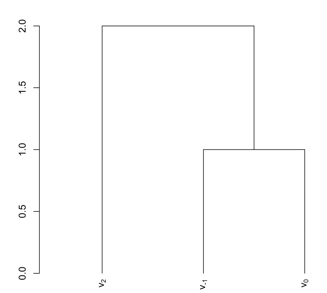
(a) Single linkage clustering dendrogram referring to the example in Section 6.0.1.

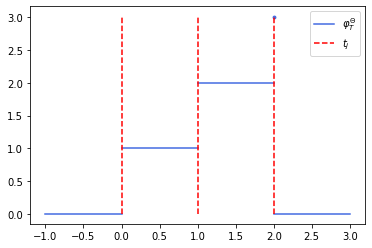
(b) In the context of the example in Section 6.0.1, we see the sum of the weight functions of the vertices going from $v_{0}$ to the root $r_{T}$: $\varphi^{\Theta_{c}}_{T}(\{v_{0}\})+\varphi^{\Theta_{c}}_{T}(\{v_{0},v_{-1}\})$. The dotted lines represent critical values.

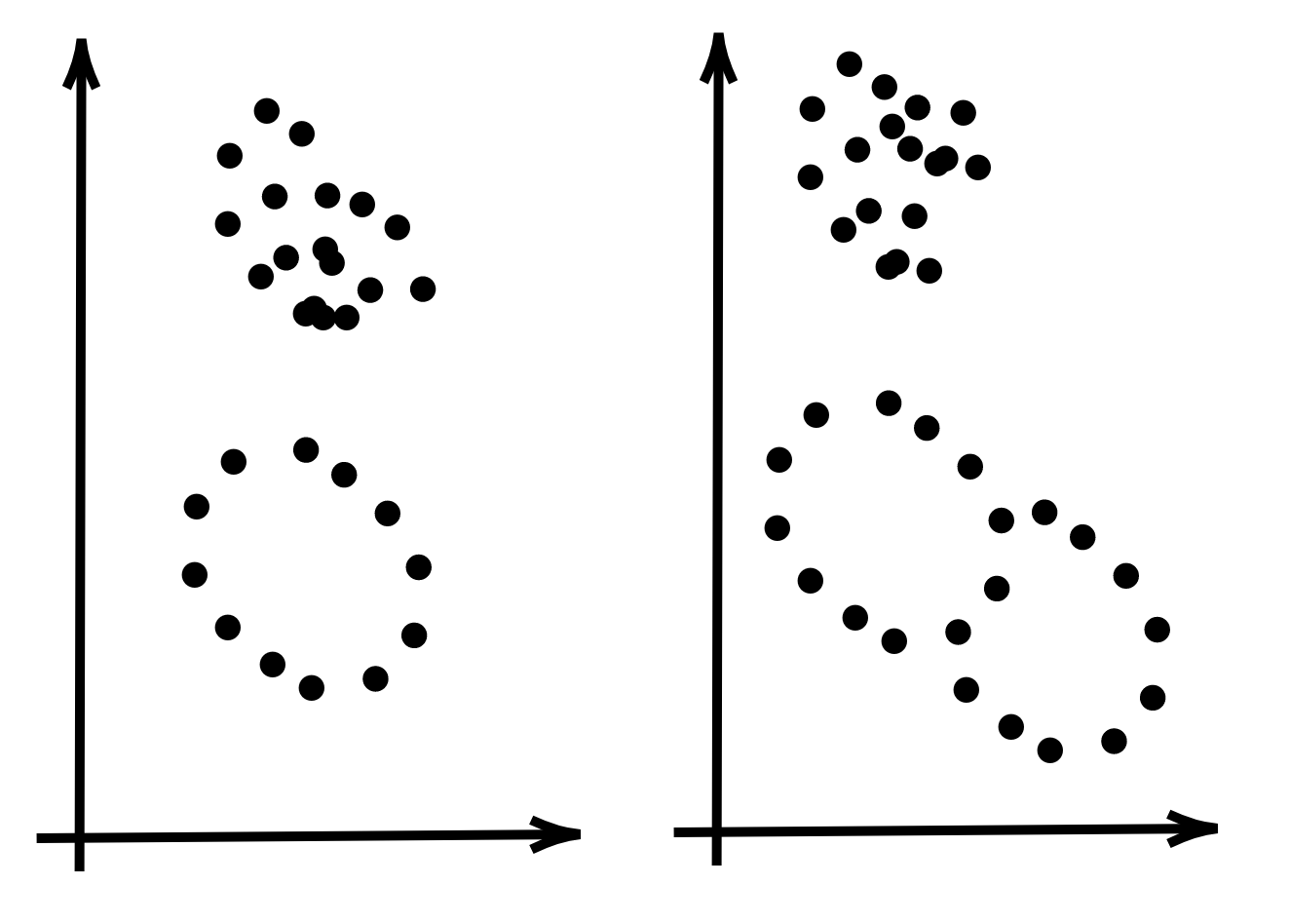
(c) Two point clouds made by two clusters each which cannot be separated by zero dimensional homology, but present different within-cluster homological information and can be distinguished by $\Theta_{1}$ defined in Section 6.0.3.

Figure 6: Plots referring to the examples in Section 6.

We close the manuscript with some examples of functions defined on display posets, to show how they can be used to capture useful information about a filtration $X_{\operatorname*{\scalerel*{\cdot}{\bigodot}}}$. In Section D we report also some simulated scenarios in which we test some of the upcoming ideas.

The general structure of the following examples is to consider a subcategory $\mathcal{B}$ of $\operatorname*{Top}$ and pick a function $\Theta:\mathcal{B}\rightarrow E$. Then, $f:D_{\pi_{0}(X_{\operatorname*{\scalerel*{\cdot}{\bigodot}}})}\rightarrow E$ is obtained as $f(a,t)=\Theta(a)$. As anticipated, we call $\varphi^{\Theta}_{T}$ the local representation of such function, and we prove that in all our examples the information contained in the functions generalizes, in some sense, the notion of merge trees. More formally, if $(T,\varphi^{\Theta}_{T})\cong(T^{\prime},\varphi^{\Theta}_{T^{\prime}})$ then $(T,h_{T})\cong(T^{\prime},h_{T^{\prime}})$. Under such hypotheses a metric to compare $(T,\varphi^{\Theta}_{T})$ and $(T^{\prime},\varphi^{\Theta}_{T^{\prime}})$ can be pulled back to compare objects of the form $(T,h_{T},\varphi_{T})$ - or, equivalently, $f\in L_{1}(D_{\pi_{0}(X_{\operatorname*{\scalerel*{\cdot}{\bigodot}}})},E)$ and $g\in L_{1}(D_{\pi_{0}(Y_{\operatorname*{\scalerel*{\cdot}{\bigodot}}})},E)$.

We immediately stress that many of the upcoming functions do not lie in $L_{p}(D_{\pi_{0}(X_{\operatorname*{\scalerel*{\cdot}{\bigodot}}})},E)$, for some $D_{\pi_{0}(X_{\operatorname*{\scalerel*{\cdot}{\bigodot}}})}$, as:

$$\lim_{x\rightarrow+\infty}d(f\circ(h_{\mid U_{\infty}})^{-1}(x),0)>0.$$

However, in Section B we discuss how these examples can be modified to fit into the proposed framework.

6.0.1 Cardinality of Clusters

Consider the case of a merge tree $\mathcal{M}(\pi_{0}(X_{\operatorname*{\scalerel*{\cdot}{\bigodot}}}))=(T,h_{T})$, with $X_{\operatorname*{\scalerel*{\cdot}{\bigodot}}}$ being the Céch filtration of the point cloud $\{x_{1},\ldots,x_{n}\}$. Sensible information that one may want to track down along $\pi_{0}(X_{\operatorname*{\scalerel*{\cdot}{\bigodot}}})$ is the cardinality of the clusters. Thus we can take $\Theta_{c}:FSets\rightarrow\mathbb{R}_{\geq 0}$, defined on all finite sets ($Fsets$) considered with the discrete topology, defined as $\Theta_{c}(\{x_{j,1},\ldots,x_{j,n_{j}}\})=n_{j}$. As a consequence, we have $\varphi^{\Theta}_{T}(e)=m\chi_{[t_{i},t_{j})}$, for some positive cardinality $m$ and some critical points $t_{i},t_{j}$. Note that, clearly, $\operatorname*{supp}(\varphi^{\Theta_{c}}_{T}(e))=[t_{i},t_{j}]$. Thus if we have $(T,\varphi^{\Theta_{c}}_{T})\cong(T^{\prime},\varphi^{\Theta_{c}}_{T^{\prime}})$ then $(T,h_{T})\cong(T^{\prime},h_{T^{\prime}})$.

We now make a concrete example - Figure 6(a) and Figure 6(b). Consider the finite set $\{v_{-1}=-1,v_{0}=0,v_{2}=2\}$ and build the abstract merge tree and the single linkage hierarchical clustering dendrogram. Abstract merge tree is given by $a_{t}=\{\{v_{-1}\},\{v_{0}\},\{v_{2}\}\}$ for $t\in[0,1)$, $a_{t}=\{\{v_{-1},v_{0}\},\{v_{2}\}\}$ for $t\in[1,2)$ and $a_{t}=\{\{v_{-1},v_{0},v_{2}\}\}$ for $t\geq t^{+}=2$. With maps given by $a\mapsto b$ with $a\subset b$.

The associated merge tree $(T,h_{T})$ - see Figure 6(a) - can be represented with the vertex set $V_{T}=\{\{v_{-1}\},\{v_{0}\},\{v_{2}\},\{v_{-1},v_{0}\},\{v_{-1},v_{0},v_{2}\},r_{T}\}$. The leaves are $\{v_{-1}\},\{v_{0}\}$ and $\{v_{2}\}$; the children of $\{v_{-1},v_{0}\}$ are $\{v_{-1}\}$ and $\{v_{0}\}$, and the ones of $\{v_{-1},v_{0},v_{2}\}$ are $\{v_{-1},v_{0}\}$ and $\{v_{2}\}$. The height function $h_{T}$ is given by $h_{T}(\{v_{i}\})=0$ for $i=-1,0,2$, $h_{T}(\{v_{-1},v_{0}\})=1$, $h_{T}(\{v_{-1},v_{0},v_{2}\})=2$ and $h_{T}(r_{T})=+\infty$.

Consider $\Theta_{c}$. The local representation $\varphi^{\Theta_{c}}_{T}$ of the induced function is thus the following: $\varphi^{\Theta_{c}}_{T}(\{v_{i}\})=\chi_{[0,1)}$ for $i=-1,0$, $\varphi^{\Theta_{c}}_{T}(\{v_{2}\})=\chi_{[0,2)}$, $\varphi^{\Theta_{c}}_{T}(\{v_{-1},v_{0}\})=2\chi_{[1,2)}$ and $\varphi^{\Theta_{c}}_{T}(\{v_{-1},v_{0},v_{2}\})=3\chi_{[2,+\infty)\}}$. See Figure 6(b).

6.0.2 Measure of Sublevel Sets

Now consider $U\subset\mathbb{R}^{m}$ convex bounded open set, with $\overline{U}$ being its topological closure, and let $\mathcal{L}$ be the Lebesgue measure in $\mathbb{R}^{m}$. Let $f:\overline{U}\rightarrow\mathbb{R}$ be a tame (Chazal et al., 2016) continuous function. Consider the sublevel set filtration $X_{t}=f^{-1}((-\infty,t])$ with $\pi_{0}(X_{t})=\{U^{t}_{1},\ldots,U^{t}_{n}\}$. Here the tameness condition is simply asking that $\pi_{0}(X_{\operatorname*{\scalerel*{\cdot}{\bigodot}}})$ is a finite constructible persistent set, and thus a finite abstract merge tree. Call $\psi_{t}^{t^{\prime}}$ the functions $\psi_{t}^{t^{\prime}}=X_{t\leq t^{\prime}}$. We set $\Theta_{\mathcal{L}}=\mathcal{L}:\mathcal{B}(\mathbb{R}^{n})\rightarrow\mathbb{R}_{\geq 0}$ with $\mathcal{B}(\mathbb{R}^{n})$ being the Borel $\sigma$-algebra of $\mathbb{R}^{n}$. So that we can always take: $\Theta_{\mathcal{L}}(U^{t}_{i})=\mathcal{L}(U^{t}_{i})$.

Proposition 12

If we have $(T,\varphi^{\Theta_{\mathcal{L}}}_{T})\cong(T^{\prime},\varphi^{\Theta_{\mathcal{L}}}_{T^{\prime}})$ then $(T,h_{T})\cong(T^{\prime},h_{T^{\prime}})$.

Proof  Let $(T,h_{T})$ being the merge tree representing $\pi_{0}(X_{\operatorname*{\scalerel*{\cdot}{\bigodot}}})$, and $\varphi^{\Theta_{\mathcal{L}}}_{T}$ the local representation of the associated function. Since $f$ is continuous, for and edge $e=(v,v^{\prime})\in E_{T}$ spanning from height $h_{T}(v)=t_{i}$ to $h_{T}(v^{\prime})=t_{j}$, we can prove that $\operatorname*{supp}(\varphi^{\Theta_{\mathcal{L}}}_{T}(e))=[t_{i},t_{j}]$. We know that $v$ is associated to a connected component $U^{t_{i}}_{k}$, for some $k$. If $v$ represents the merging of two or more path connected components $U^{t_{i}-\varepsilon}_{k_{1}}$ and $U^{t_{i}-\varepsilon}_{k_{2}}$, for some small $\varepsilon>0$, with $\mathcal{L}(U^{t_{i}-\varepsilon}_{k_{1}}),\mathcal{L}(U^{t_{i}-\varepsilon}_{k_{2}})>0$, then, since $U^{t_{i}-\varepsilon}_{k_{1}},U^{t_{i}-\varepsilon}_{k_{2}}\subset U^{t_{i}}_{k}$, we have $\mathcal{L}(U^{t_{i}}_{k})>0$. Thus if we prove the statement for $v$ leaf, we are done. So, suppose $v$ is a leaf and consider $x_{0}\in U^{t_{i}}_{k}$. We know $f(x_{0})=t_{i}$. By the continuity of $f$, for every $\varepsilon>0$ there is $\delta>0$ such that if $\mid\mid x-x_{0}\mid\mid<\delta$, then $f(x_{0})\leq f(x)<f(x_{0})+\varepsilon$. Since $\{x\in\overline{U}\mid\mid\mid x-x_{0}\mid\mid<\delta\}$ is convex (and so path connected), then it is contained in $\psi_{t_{i}}^{t_{i}+\varepsilon}(U^{t_{i}}_{k})$. Moreover, since it contains the non-empty open set $\{x\in U\mid\text{ }\mid\mid x-x_{0}\mid\mid<\delta\}$, we have $\mathcal{L}(\psi_{t_{i}}^{t_{i}+\varepsilon}(U^{t_{i}}_{k}))>0$ for every $\varepsilon>0$. As a consequence, $\operatorname*{supp}(\varphi^{\Theta_{\mathcal{L}}}_{T}(e))=[t_{i},t_{j}]$.  

Again we make a quick hands-on example. Consider the function $f=\mid\mid x\mid-1\mid$ defined on the interval $[-2,2]$. Let $\pi_{0}(X_{t})=\pi_{0}(f^{-1}((-\infty,t]))$. Let $(T,h_{T})$ be the merge tree associated to the sequence $\pi_{0}(X_{\operatorname*{\scalerel*{\cdot}{\bigodot}}})$. Now we obtain the local representation $\varphi^{\Theta_{\mathcal{L}}}_{T}(e_{i})$.

We have $\varphi^{\Theta_{\mathcal{L}}}_{T}(e_{1})=\mid 1+t-1+t\mid=2t$ for $t\in[0,1)$, and $0$ otherwise. Clearly $\varphi^{\Theta_{\mathcal{L}}}_{T}(e_{1})=\varphi^{\Theta_{\mathcal{L}}}_{T}(e_{2})$. Lastly $\varphi^{\Theta_{\mathcal{L}}}_{T}(r_{T})=4\chi_{[2,+\infty)}$.

6.0.3 Homological Information

Lastly we propose a function $\Theta_{p}$ to combine homological information of different dimensions (Hatcher, 2000) obtaining dendrograms which are closely related to the barcode decorated merge trees defined by Curry et al. (2022). We consider the topological spaces with $p$-th homology of finite type, that is, their $p$-th homology group is finitely generated, and collect all the spaces with finitely generated $1,\ldots,p$-th homology groups in the set $\operatorname*{FTop}_{p}$. Consider $\Theta_{p}:\operatorname*{FTop}_{p}\rightarrow\mathbb{N}\times\ldots\times\mathbb{N}$ defined on a topological space $U$ as $\Theta_{p}(U)=(\dim(H_{0}(U;\mathbb{K}),\ldots,\dim(H_{p}(U;\mathbb{K}))$, with $H_{p}(U;\mathbb{K})$ being the $p$-th homology group of $U$ with coefficients in the field $\mathbb{K}$. Note that, by definition, generators of homology groups of $U$ lie inside a connected component. In this way we are able to track if in a path connected component there are some kind of holes arising or dying, and thus collecting a more complete set of topological invariants which capture the shape of each connected component, which could be useful in situations like the one depicted in Figure 6(c). From another point of view, at every step along a filtration, we are decomposing homological information of a topological space by means of its connected components.

Note that we clearly have $(T,\varphi^{\Theta_{p}}_{T})\cong(T^{\prime},\varphi^{\Theta_{p}}_{T^{\prime}})$ implying $(T,h_{T})\cong(T^{\prime},h_{T^{\prime}})$. In fact $\operatorname*{FTop}_{p}\xrightarrow{\Theta_{p}}\mathbb{N}\times\ldots\times\mathbb{N}\xrightarrow{\pi_{1}}\mathbb{N}$ is $\Theta_{1}$ - with $\pi_{1}$ being the projection on the first component.

7 Conclusions

We develop a framework to work with functions defined on different merge trees. As motivated in the manuscript, we argue that these kinds of topological summaries can succeed in situations where persistence diagrams and merge trees alone are not effective. They also provide a great level of versatility because of the wide range of additional information that can be extracted from data. We define a metric structure which has suitable stability properties and is feasible if the number of leaves is not too high and we test it in simulated scenarios to prove its effectiveness.

The main drawback of the framework is that the deformation between two functions is not guaranteed to always produce a function at the intermediate steps i.e. the metric space of local representation of functions is embedded in a bigger dendrograms space, but geodesics between points in general are not contained in this subspace. We believe that there is always at least one geodesic which remains in this subspace. Investigating such claim will be the object of future works. In case this does not hold true, it may limit the intrinsic statistical tools that can be defined in this space: should Frechét means exists, for instance, it is not guaranteed that they are functions.

Outline of the Appendix

Section A briefly motivates the use of merge trees over more traditional TDA’s techniques with a couple of examples, introducing also some problems which can be solved by considering functions on merge trees. In Section B we describe how the examples presented in Section 6 can be modified in order to fall back into the admissible function spaces. In Section C we take a little detour to showcase why all the machinery we set up to work with functions defined on merge trees does not work with persistence diagrams. Section D presents some simulated scenarios to test some of the functions defined in Section 6. Section E contains the proofs of the results in the paper.

A Why Using Trees

We want to give some motivation to propel the use of merge trees and functions defined on merge trees over persistence diagrams, in certain situations. We give only two brief examples since a similar topic is already tackled for instance in Elkin and Kurlin (2021), Smith and Kurlin (2022), Kanari et al. (2020), Curry et al. (2021) and Curry et al. (2022).

A.1 Point Clouds

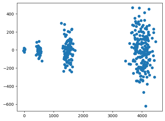
(a) First point cloud.

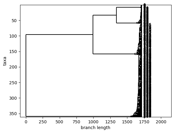
(b) First dendrogram.

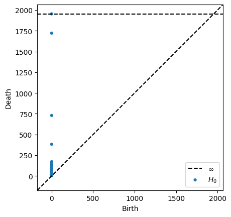
(c) First PD.

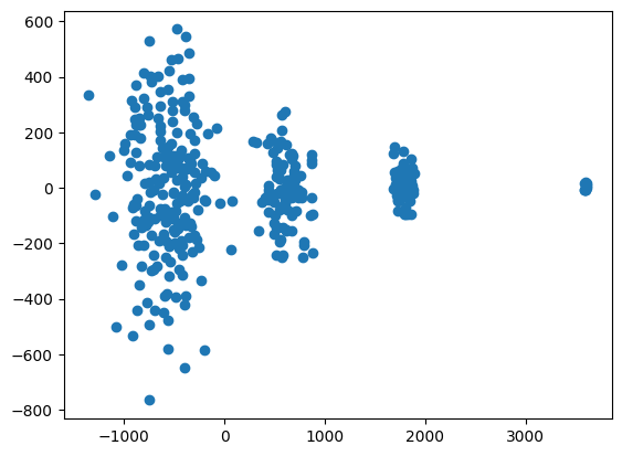
(d) Second point cloud.

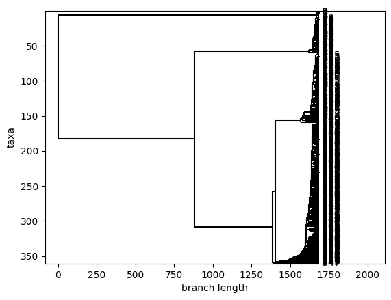
(e) Second dendrogram.

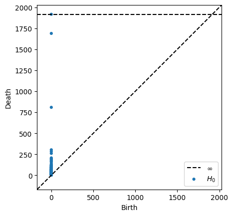
(f) Second PD.

Figure 7: Data clouds, hierarchical clustering dendrograms and PDs involved in the first example.

Given a point cloud $C=\{x_{1},\ldots,x_{n}\}$ in $\mathbb{R}^{n}$ there are many ways in which one can build a family of simplicial complexes (Edelsbrunner and Harer, 2008) whose vertices are given by $C$ itself and whose set of higher dimensional simplices gets bigger and bigger. A standard tool to do so is the Vietoris-Rips filtration of $C$ (Edelsbrunner and Harer, 2008), as are $\alpha$ filtrations, Céch filtrations etc..

As we are interested only in path connected components we restrict our attention to $0$ dimensional simplices (points) and $1$ dimensional simplices (edges). With such restrictions, many of the aforementioned filtrations become equivalent and amount to having a family of graphs $\{C_{t}\}_{t\geq 0}$ such that the vertex set of $C_{t}$ is $C$ and the edge between $x_{i}$ and $x_{j}$ belongs to $C_{t}$ if and only if $d(x_{i},x_{j})<t$. Thus, the set of edges of $C_{t^{\prime}}$ contains the set of edges of $C_{t}$, with $t\leq t^{\prime}$; while the set of vertices is always $C$. Note, for instance, that the path connected components of $C_{t}$ are equivalent to the ones of $X_{t/2}$ with $X_{\operatorname*{\scalerel*{\cdot}{\bigodot}}}$ being the Céch filtration built in Section 2.1. Along this filtration of graphs, the closest points become connected first and the farthest ones at last. It is thus reasonable to interpret the path connected components of $C_{t}$ as clusters of the point cloud $C$. In order to choose the best “resolution” to look at clusters, i.e. in order to choose $t$ and use $C_{t}$ to infer the clusters, statisticians look at the merge tree $\mathcal{M}(\pi_{0}(C_{t})_{t\geq 0})$, which is called hierarchical clustering dendrogram. More precisely, $\mathcal{M}(\pi_{0}(C_{t})_{t\geq 0})$ is the single linkage hierarchical clustering dendrogram. Note that $\pi_{0}(X_{\operatorname*{\scalerel*{\cdot}{\bigodot}}})$ is a regular abstract merge tree.

Suppose, instead, that we have the persistence diagram obtained from $\{\pi_{0}(C_{t})\}_{t\in\mathbb{R}_{\geq 0}}$. Persistence diagrams are made of points in $\mathbb{R}^{2}$ whose coordinates $(b,d)$ represent the value of $t$ at which a certain path-connected component appears and the value of $t$ at which that component merges with a component which appeared before $b$. Each point in the point cloud is associated to a path connected component but, in general, we have no way to distinguish between points of the diagram associated to path connected components which are proper clusters and points of the diagrams associated to outliers.

Now, consider the single linkage dendrograms and the zero dimensional PDs obtained from point clouds as in Figure 7. The persistence diagrams (in Figure 7(c) and Figure 7(f)) are very similar, in fact they simply record that there are four major clusters which merge at similar times across the Vietoris-Rips filtrations of the two point clouds. The hierarchical dendrograms, instead, are clearly very different since they show that in the first case (Figure 7(a), Figure 7(b), Figure 7(c)) the cluster with most points is the one which is more separated from the others in the point cloud; while in the second case (Figure 7(d), Figure 7(e), Figure 7(f)) the two bigger clusters are the first that get merged and the farthest cluster of points on the right could be considered as made by outliers. In many applications it would be important to distinguish between these two scenarios, since the two main clusters get merged at very different heights on the respective dendrograms.

These observations are formalized in Curry et al. (2021), with the introduction of the tree realization number with is a combinatorial description of how many merge trees share a particular persistence diagram. With hierarchical clustering dendrograms with $n$ leaves, such number is $n!$: all leaves are born at height $0$, and so, at the first merging point, each of the $n$ leaves can merge with any of the $n-1$ remaining ones. At the following merging step we have $n-1$ clusters and each one of them can merge with the other $n-2$ etc..

A.2 Real Valued Functions

Given a continuous function $f:[a,b]\rightarrow\mathbb{R}$ we can extract the merge tree $\mathcal{M}(\pi_{0}(X_{\operatorname*{\scalerel*{\cdot}{\bigodot}}}))$, with $X_{\operatorname*{\scalerel*{\cdot}{\bigodot}}}$ being the sublevel set filtration (see Section 2.1 and Section 3.2): we obtain a merge tree that tracks the evolution of the path connected components of the sublevel sets $f^{-1}((-\infty,t])$. For a visual example see Figure 8(b). Pegoraro and Secchi (2021) shows that $\pi_{0}(X_{\operatorname*{\scalerel*{\cdot}{\bigodot}}})$ is a regular merge tree.

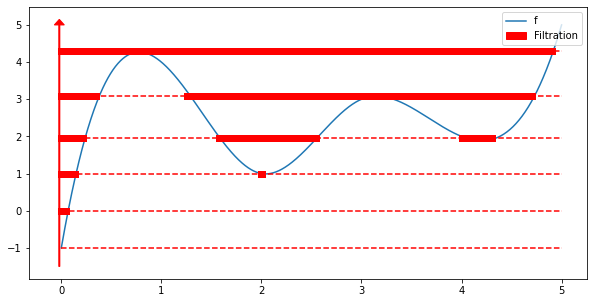
(a) Sublevel sets of a function

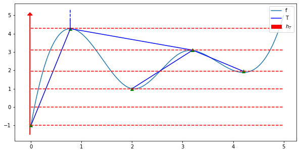
(b) A function with its associated merge tree.

Figure 8: Merge Trees of Functions

We use this example to point out two facts. First PDs may not be able to distinguish functions one may wish to distinguish, as made clear by Figure 9. Second, Proposition 1 of Pegoraro and Secchi (2021) states that if one changes the parametrization of a function by means of homeomorphisms, then, both the associated merge tree and persistence diagram do not change. A consequence of such result is that one can shrink or spread the domain of the function $f:[a,b]\rightarrow\mathbb{R}$ with reasonably regular functions, without changing its merge tree (and PD). There are cases in which such property may be useful but surely there are times when one may want to distinguish if an oscillation lasted for a time interval of $10^{-5}$ or $10^{5}$. The measure related function defined in Section 6 can solve this issue.

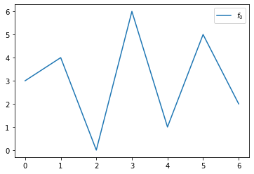
(a) A function $f_{0}$.

(b) The $0$-dimensional persistence diagram of $f_{0}$.

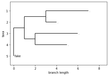
(c) The merge tree of $f_{0}$.

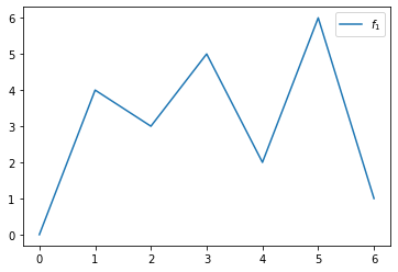
(d) A function $f_{1}$.

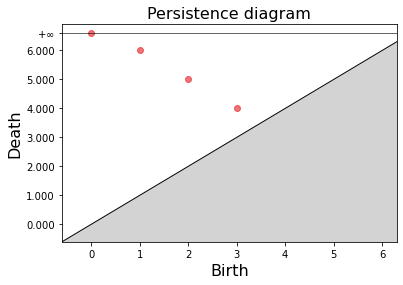
(e) The $0$-dimensional persistence diagram of $f_{1}$.

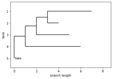
(f) The merge tree of $f_{1}$.

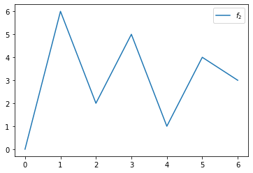
(g) A function $f_{2}$.

(h) The $0$-dimensional persistence diagram of $f_{2}$.

(i) The merge tree of $f_{2}$.

(j) A function $f_{3}$.

(k) The $0$-dimensional persistence diagram of $f_{3}$.

(l) The merge tree of $f_{3}$.

Figure 9: We compare four functions; they are all associated to the same $PD$ but to different merge trees. Functions are displayed in the first column and on each row we have on the centre the associated $PD$ and on the right the merge tree.

B Normalizing and Truncating Functions

We devote this section to describe a way in which the functions defined in Section 6 can fit into our framework.

We start with a very useful couple of results. Note that the piece of notation $sub_{T}(v)$ is defined in 8.

Proposition 13 (Extension/Truncation)

Take $(T,\varphi_{T})$ and $(T^{\prime},\varphi_{T^{\prime}})$. Suppose $r_{T}$ and $r_{T^{\prime}}$ are of order $1$ and there is a splitting $\{(v,r_{T})\}\rightarrow\{(v,v^{\prime}),(v^{\prime},r_{T})\}$ and $\{(w,r_{T^{\prime}})\}\rightarrow\{(w,w^{\prime}),(w^{\prime},r_{T^{\prime}})\}$ giving the dendrograms $(G,h_{G})$ and $(G^{\prime},h_{G^{\prime}})$. Suppose moreover that $\varphi_{G}((v^{\prime},r_{T}))=\varphi_{G^{\prime}}((w^{\prime},r_{G}))$. Then $d_{E}(T,T^{\prime})=d_{E}(sub_{G}(v^{\prime}),sub_{G^{\prime}}(w^{\prime}))$.

Proof 

Consider a minimizing mapping $M$ between $G$ and $G^{\prime}$.

Apply the deletions described by $M$ both on $G$ and on $G^{\prime}$ obtaining the merge trees $G_{M}$ and $G^{\prime}_{M}$. After such deletions the vertices $r_{G}$ and $r_{G^{\prime}}$ are still in the resulting trees, for they cannot be removed in any way. Moreover, if $(v^{\prime},w^{\prime})\notin M$ then neither $v^{\prime}$ nor $w^{\prime}$ can be deleted. In fact, for any $4$ positive numbers $n_{1},n_{2},n_{3},n_{4}$ we have:

$$\mid n_{1}+n_{2}-(n_{3}+n_{4})\mid\leq n_{1}+n_{3}+\mid n_{2}-n_{4}\mid$$

thus instead of deleting $v^{\prime}$ with cost $n_{1}$ and $w^{\prime}$ with cost $n_{3}$ and then shrinking two edges of the form $e=(a,r_{G})$ and $e^{\prime}=(b,r_{G^{\prime}})$ with weights $n_{2}$ and $n_{4}$ is better to merge $(a,v^{\prime})$ with $(v^{\prime},r_{G})$ and $(b,w^{\prime})$ with $(w^{\prime},r_{G^{\prime}})$ and then shrink them.

Thus, whatever edge of the form $e=(a,r_{G})$ remains contains, as a merged edge, also $(v^{\prime},r_{G})$. And the same for $e^{\prime}=(b,r_{G^{\prime}})$. By construction $e$ is matched with $e^{\prime}$. Since $\varphi_{G_{M}}(e)=\varphi_{G}((v^{\prime},r_{G}))\ast\ldots$ and $\varphi_{G^{\prime}_{M}}(e)=\varphi_{G}((w^{\prime},r_{G^{\prime}}))\ast\ldots$, when computing the cost of shrinking $e$ on $e^{\prime}$, by (P4), $\varphi_{G}((v^{\prime},r_{G}))$ and $\varphi_{G}((w^{\prime},r_{G^{\prime}}))$ cancel out.

Thus $d_{E}(T,T^{\prime})=d_{E}(G,G^{\prime})=d_{E}(sub_{G}(v^{\prime}),sub_{G^{\prime}}(w^{\prime}))$.  

The proof of 13, together with the definition of mappings (see LABEL:pegoraro2023edit) also yields the following corollary.

Corollary 5

Given $(T,\varphi_{T})$ and $(T^{\prime},\varphi_{T^{\prime}})$. If $r_{T}$ and $r_{T^{\prime}}$ are of order $1$, for any minimizing mappings $M$, then neither $(v,r_{T})$ or $(w,r_{T^{\prime}})$ are deleted and we have $\#\max M=1$.

Consider $f,g:D_{\pi_{0}(X_{\operatorname*{\scalerel*{\cdot}{\bigodot}}})}\rightarrow E$. If $\parallel f_{\mid U_{\infty}}-g_{\mid U_{\infty}}\parallel_{L_{1}(U_{\infty},E)}=\infty$, then there is no point in comparing such functions and any attempt to embed those functions into $L_{1}(\mathbb{R},E)$ implies losing infinite variability/information at least for one of the two functions. In fact, at least one between $f_{\mid U_{\infty}}$ and $g_{\mid U_{\infty}}$ has norm equal to $\infty$ and any approximation we make of that function with a function of finite norm, would be at infinite distance from the original function. However, if we deem that the information contained in $f_{\mid U_{\infty}}$ and $g_{\mid U_{\infty}}$ after a certain height is negligible, we can always put $f$ to $0\in E$ after some $K\geq\max h_{T}$, with $\mathcal{M}(\pi_{0}(X_{\operatorname*{\scalerel*{\cdot}{\bigodot}}}))=(T,h_{T})$. We indicate extension with $f_{\mid U_{\infty}}\cdot\chi_{[\max h_{T},K]}$ with an abuse of notation, and we refer to it as the truncation of $f$ at height $K$. Then, call $f_{\mid K}$ the function obtained as $(f_{\mid K})_{\mid U}:=f_{\mid U}$ for all $U\in\mathcal{U}(D_{\pi_{0}(X_{\operatorname*{\scalerel*{\cdot}{\bigodot}}})})$, $U\neq U_{\infty}$, and $(f_{\mid K})_{\mid U_{\infty}}:=f_{\mid U_{\infty}}\cdot\chi_{[\max h_{T},K]}$. Clearly $f_{\mid K}\in L_{1}(D_{\pi_{0}(X_{\operatorname*{\scalerel*{\cdot}{\bigodot}}})},E)$.

The examples in Section 6, however allow also for a different approach. Suppose we have $f:D_{\pi_{0}(X_{\operatorname*{\scalerel*{\cdot}{\bigodot}}})}\rightarrow E$, $g:D_{\pi_{0}(Y_{\operatorname*{\scalerel*{\cdot}{\bigodot}}})}\rightarrow E$, with the height functions of the display posets being respectively $h^{f}$ and $h^{g}$, and suppose there is $K\in\mathbb{R}$ such that:

$$f\circ(h^{f}_{\mid U^{f}_{\infty}})^{-1}(x)=g\circ(h^{g}_{\mid U^{g}_{\infty}})^{-1}g(x)$$

for $x>K$. That is, $f,g$ are definitively equal going upwards towards the roots. Then, let $(T,h_{T})$ and $(G,h_{G})$ be the merge trees associated to the sublevel set filtrations of $f$ and $g$ respectiely. We can split $e_{f}=(v,r_{T})\in E_{T}$ into $e^{\prime}_{f}=(v,v^{\prime})$, $e^{\prime\prime}_{f}=(v^{\prime},r_{T})$ and $e_{g}=(w,r_{G})\in E_{G}$ into $e^{\prime}_{g}=(w,w^{\prime})$, $e^{\prime\prime}_{g}=(w^{\prime},r_{G})$, so that $h^{f}(v^{\prime})=h^{g}(w^{\prime})=K$. Let $(T^{\prime},h_{T^{\prime}})$ and $(G^{\prime},h_{G^{\prime}})$ be the merge trees obtained with such splittings. If we call $\varphi_{T^{\prime}}$ and $\varphi_{G^{\prime}}$ the local representations of $f$ on $T^{\prime}$ and $g$ on $G^{\prime}$, respectively, we have: $\parallel\varphi_{T^{\prime}}(e_{f}^{\prime\prime})-\varphi_{G^{\prime}}(e_{g}^{\prime\prime})\parallel_{L_{1}(\mathbb{R},E)}=0$. Thus we are in the position to apply 13 to $T^{\prime}$ and $G^{\prime}$.

In other words, if we can modify $\Theta$ so that

$$\Theta\circ(h^{f}_{\mid U^{f}_{\infty}})^{-1}(x)=\Theta\circ(h^{g}_{\mid U^{g}_{\infty}})^{-1}g(x)$$

for some $K$ and $x>K$ then $d_{E}(f,g)$ can be defined as $d_{E}(f_{\mid K},g_{\mid K})$. We will do so requiring that $\Theta$ is definitively equal to some fixed constant.

Now we consider the different $\Theta$ employed in Section 6:

• $\Theta_{1}$: in this case we have $\Theta_{1}\equiv 1$ and thus $\Theta^{1}$ is definitively constant and equal to $1$;

• $\Theta_{c}$: $\Theta_{c}$ is employed when we build clustering dendrograms and so definitively it is equal to the cardinality of the starting point cloud. Thus we can normalize $\Theta_{c}$ obtaining $\Theta_{c}^{n}$ which expresses the cardinality of the clusters as a percentage of the cardinality of the point cloud i.e. the measure of the clusters wrt the uniform measure on the point cloud. Clearly such function is definitively equal to $1$;

• $\Theta_{\mathcal{L}}$: when we start from a function $f:X\rightarrow\mathbb{R}$ which is bounded and defined on $X\subset\mathbb{R}^{n}$ bounded, then $X_{t}=X$ for $t$ big enough and so $\Theta_{\mathcal{L}}$ is definitively constant and equal to $\Theta_{\mathcal{L}}(X)$. Again we can normalize $\Theta_{\mathcal{L}}$, obtaining $\Theta_{\mathcal{L}}^{n}$ which expresses the measure of path connected components as a percentage of the measure of $\mathcal{L}(X)$.

• $\Theta_{p}$: for this function it really depends on the chosen filtration and, in particular, if there is the possibility of having homology classes with death time $+\infty$ in $p$-dimensional homology, $p>0$. However, if $H_{p}(U;\mathbb{K})=0$, $U\in\pi_{0}(X_{t})$ for all $t$ big enough, as is the case, for instance, with the Céch filtration, or other filtrations of a simply connected space, we have no issues. In fact we know that, by construction, $H_{0}(U;\mathbb{K})=\mathbb{K}$, $U\in\pi_{0}(X_{t})$ for $t$ big enough. Thus there is $K$ big enough so that $\Theta_{p}\equiv(1,0)$ for $x>K$.

For what we have said previously then we can choose $K$ big enough and define $d_{E}(f,g):=d_{E}(f_{\mid K},g_{\mid K})$ for any $f$ induced by the normalized functions $\Theta_{1}$, $\Theta_{c}^{n}$ and $\Theta_{\mathcal{L}}^{n}$.

In other words, suppose that we want to work, for instance, with $\Theta_{\mathcal{L}}^{n}$ to analyze a data set of functions. For any couple of functions $f:X\rightarrow\mathbb{R}$ and $g:Y\rightarrow\mathbb{R}$ we obtain the abstract merge trees $\pi_{0}(X_{\operatorname*{\scalerel*{\cdot}{\bigodot}}})$ and $\pi_{0}(Y_{\operatorname*{\scalerel*{\cdot}{\bigodot}}})$ with sublevel set filtrations and the corresponding functions:

$$f^{\Theta_{\mathcal{L}}^{n}}(p)=\Theta_{\mathcal{L}}^{n}((a,t))=\mathcal{L}(a)/\mathcal{L}(X)$$

for $p=(a,t)\in D_{\pi_{0}(X_{\operatorname*{\scalerel*{\cdot}{\bigodot}}})}$ and

$$g^{\Theta_{\mathcal{L}}^{n}}(q)=\Theta_{\mathcal{L}}^{n}((b,t))=\mathcal{L}(b)/\mathcal{L}(Y)$$

for $q=(b,t)\in D_{\pi_{0}(Y_{\operatorname*{\scalerel*{\cdot}{\bigodot}}})}$. Then we choose $K$ big enough $\Theta_{\mathcal{L}}^{n}((a,t))=1=\Theta_{\mathcal{L}}^{n}((b,t))$ for $t\geq K$. Thus we can truncate these functions from $K$ upwards and obtain the local representations $\varphi_{T}^{\Theta_{\mathcal{L}}^{n}}$ and $\varphi_{G}^{\Theta_{\mathcal{L}}^{n}}$ of the truncated functions. Note that $\operatorname*{supp}(\varphi_{T}^{\Theta_{\mathcal{L}}^{n}}((v,r_{T})))=[\max h_{T},K]$ and $\operatorname*{supp}(\varphi_{G}^{\Theta_{\mathcal{L}}^{n}}((w,r_{G})))=[\max h_{G},K]$.

By 13 we are guaranteed that this truncation process:

1. does not depend on $K$, in the following sense. Suppose we have a third function $r:H\rightarrow\mathbb{R}$ such that $r^{\Theta_{\mathcal{L}}^{n}}(u)=\Theta_{\mathcal{L}}^{n}((c,t))<1$ for some $t>K$. While $f^{\Theta_{\mathcal{L}}^{n}}$ and $g^{\Theta_{\mathcal{L}}^{n}}$ can be truncated at height $K$, for $r^{\Theta_{\mathcal{L}}^{n}}$ we must consider some $K^{\prime}>K$ to compute $d_{E}(f^{\Theta_{\mathcal{L}}^{n}}_{\mid K^{\prime}},r^{\Theta_{\mathcal{L}}^{n}}_{\mid K^{\prime}})$. However, we have :

   $$d_{E}(f^{\Theta_{\mathcal{L}}^{n}}_{\mid K^{\prime}},g^{\Theta_{\mathcal{L}}^{n}}_{\mid K^{\prime}})=d_{E}(f^{\Theta_{\mathcal{L}}^{n}}_{\mid K},g^{\Theta_{\mathcal{L}}^{n}}_{\mid K});$$

2. moreover, comparing the truncated functions $f^{\Theta_{\mathcal{L}}^{n}}_{\mid K}$ is exactly the same as comparing the original functions $f^{\Theta_{\mathcal{L}}^{n}}$ with $d_{E}$.

C Functions on Merge Trees vs Functions on PDs

(a) The functions $f$ and $g$ in Section C; with $\varepsilon=0.3$.

(b) In the context of the example in Section C, we report $\varphi^{\Theta_{\mathcal{L}}}_{T}(v_{1})$ and $\varphi^{\Theta_{\mathcal{L}}}_{T}(v_{-0.5})$. The dotted lines represent critical values.

We make one example which shows what could happen if we try to define functions on PDs in the same way we do for merge trees. In particular, the elder rule, via the instability of the persistence pairs, makes it very difficult to add pieces of information to persistence diagrams in a stable way.

Consider the following functions, plotted in Figure 10(a), defined on $[-1,2]$:

$$f(x)=\mid x-1\mid+\varepsilon \text{ if }x\geq 0$$

$$f(x)=\mid 2x-1\mid \text{ if }x<0$$

and

$$g(x)=\mid x-1\mid \text{ if }x\geq 0$$

$$g(x)=\mid 2x-1\mid+\varepsilon \text{ if }x<0$$

for a fixed $\varepsilon>0$.

Let $(T,h_{T})$ and $(T^{\prime},h_{T^{\prime}})$ be the merge trees associated to the sublevel set filtrations of $f$ and $g$; moreover let $\varphi^{\Theta_{\mathcal{L}}}_{T}$ and $\varphi^{\Theta_{\mathcal{L}}}_{T^{\prime}}$ the two respective local representations of the induced functions with $\Theta_{\mathcal{L}}$ being the Lebesgue measure on $\mathbb{R}$. Note that $\parallel f-g\parallel_{\infty}=\varepsilon$. The local minima of the functions are the points $\{-0.5,1\}$, with $f(-0.5)=0$, $f(1)=\varepsilon$, $g(-0.5)=\varepsilon$ and $g(1)=0$. Thus the merge trees have isomorphic tree structures: we represent $T$ with the vertex set $\{v_{-0.5},v_{1},v_{0},r_{T}\}$ and edges $\{(v_{-0.5},v_{0}),(v_{1},v_{0}),(v_{0},r_{T^{\prime}})\}$; and $T^{\prime}$ with vertices $\{v_{-0.5},v_{1},v_{0},r_{T^{\prime}}\}$ and edges $\{(v_{-0.5},v_{0}),(v_{1},v_{0}),(v_{0},r_{T^{\prime}})\}$. The height functions are the following: $h_{T}(v_{-0.5})=0$, $h_{T^{\prime}}(v_{-0.5})=\varepsilon$, $h_{T}(v_{1})=\varepsilon$, $h_{T^{\prime}}(v_{1})=0$ and $h_{T}(v_{0})=h_{T^{\prime}}(v_{0})=1+\varepsilon$.

Having truncated both functions at height $1+\varepsilon$, the weight functions (see Figure 10(b)) are given by: $\varphi^{\Theta_{\mathcal{L}}}_{T}(v_{-0.5})(t)=t\chi_{[0,1)}+\chi_{[1,1+\varepsilon)}$, $\varphi^{\Theta_{\mathcal{L}}}_{T}(v_{1})(t)=2(t-\varepsilon)\chi_{[\varepsilon,1+\varepsilon)}$ and $\varphi^{\Theta_{\mathcal{L}}}_{T^{\prime}}(v_{-0.5})(t)=(t-\varepsilon)\chi_{[\varepsilon,1+\varepsilon)}$ and $\varphi^{\Theta_{\mathcal{L}}}_{T^{\prime}}(v_{1})(t)=2t\chi_{[0,1)}+2\chi_{[1,1+\varepsilon)}$.

The zero-dimensional persistence diagram associated to $f$ (we name it $PD_{0}(f)$) is given by a point with coordinates $(0,+\infty)$, associated to the connected component $[-t/2-0.5,t/2-0.5]$ which is born at $t=0$, and the point $(\varepsilon,1+\varepsilon)$, associated to the component $[1-(t-\varepsilon),1+(t-\varepsilon)]$, born at level $t=\varepsilon$ and “dying” at level $t=1+\varepsilon$, due to the elder rule, since it merges an older component, being the other component born at a lower level.

For the function $g$, the persistence diagram $PD_{0}(g)$ is made by the same points, but the situation is in some sense “reversed”. In fact, the point $(0,+\infty)$ is associated to the connected component “centered” in $1$, which is $[1-t,1+t]$, and the point $(\varepsilon,1+\varepsilon)$, is associated to the component “centered” in $0.5$, that is $[-(t-\varepsilon)/2-0.5,(t+\varepsilon)/2-0.5]$.

The consequence of this change in the associations between points and the components originating the points of the diagrams is that the information regarding the two components, end up being associated to very different spatial locations in the two diagrams: $(0,+\infty)$ and $(\varepsilon,1+\varepsilon)$. And this holds for every $\varepsilon>0$. Thus it seems very hard to design a way to “enrich” $PD_{0}(f)$ and $PD_{0}(g)$ with additional information, originating the “enriched diagrams” $D_{f}$ and $D_{g}$, respectively, and design a suitable metric $d$, so that $d(D_{f},D_{g})\rightarrow 0$ as $\varepsilon\rightarrow 0$.

Instead, if we consider the edit path $\gamma$ which shrinks $v_{-0.5}\rightarrow v_{-0.5}$ and $v_{1}\rightarrow v_{1}$ we have $d_{E}((T,\varphi^{\Theta_{\mathcal{L}}}_{T}),(T^{\prime},\varphi^{\Theta_{\mathcal{L}}}_{T^{\prime}}))\leq cost(\gamma)=3\varepsilon$.

D Simulated Scenarios

Now we use two simulated data sets to put to work the frameworks defined in Section 6. The algorithm employed to compute the metric is proposed in Pegoraro (2023).

The examples are basic, but suited to assert that dendrograms and the metric $d_{E}$ capture the information we designed them to grasp. In particular, since examples in Section A.1 and Section A.2 already give insights into the role of the tree-structured information, we want to isolate and emphasize the key role of weight functions. We also deal with the problem of approximating the metric $d_{E}$ when the number of leaves in the tree structures in the data set is too big to be handled. The examples presented concern hierarchical clustering dendrograms and dendrograms representing scalar fields.

In the implementations, dendrograms are always considered with a binary tree structure, obtained by adding negligible edges, that is edges $e$ with arbitrary small $d(\varphi(e),0)$, when the number of children of a vertex exceeds $2$.

D.1 Pruning

In this section we report a way of approximating the edit distance when the number of leaves of the involved tree structures is too high, taken from Pegoraro and Secchi (2021).

If one defines a proper weight function with values in an editable space $(E,d)$ coherently with the aim of the analysis, then the value $d(\varphi_{T}(e),0)$ can be thought as the amount of information carried by the edge $e$. The bigger such value is, the more important that edge will be for the dendrogram. In fact such edges are the ones most relevant in terms of $d_{E}$. A sensible way to reduce the computational complexity of the metric $d_{E}$, losing as little information as possible, is therefore the following. Given $\varepsilon>0$ and a dendrogram $(T,\varphi_{T})$, define the following 1-step process:

• Take a leaf $l$ such that $d(\varphi_{T}(l),0)$ is minimal among all leaves; if two or more leaves have minimal weight, choose $l$ at random among them. If $d(\varphi_{T}(l),0)<\varepsilon,$ delete $l$ and ghost its father if it becomes an order $2$ vertex after removing $l$.

We set $T_{0}=T$ and we apply operation (${\cal P}_{\varepsilon}$) to obtain $T_{1}$. On the result we apply again (${\cal P}_{\varepsilon}$) obtaining $T_{2}$ and, for $n>2,$ we proceed iteratively until we reach the fixed point of the sequence $\{T_{n}\}$, which we call $P_{\varepsilon}(T)$. In this way we define the pruning operator $P_{\varepsilon}:\mathcal{T}\rightarrow\mathcal{T}$. Note that the fixed point is surely reached in a finite time since the number of leaves of each tree in the sequence is finite and non increasing along the sequence. More details on such pruning operator applied on merge trees representing the path connected components of the sublevel sets of real valued functions can be found in Pegoraro and Secchi (2021), showing in the case of merge trees that the pruning operation can be interpreted quite naturally in terms of function deformations.

If we define $\parallel T\parallel$ as $\parallel T\parallel=\sum_{e\in E_{T}}d(\varphi(e),0)$, we can quantify the (normalized) lost information with what we call pruning error ($PE$): $(\parallel T\parallel-\parallel P_{\varepsilon}(T)\parallel)/\parallel T\parallel$.

Figure 11: Pruning of a weighted tree: in red the deletions and in yellow the ghostings.

D.2 Hierarchical Clustering Dendrograms

We consider a data set of $30$ points clouds in $\mathbb{R}^{2}$, each with $150$ or $151$ points. Point clouds are generated according to three different processes and are accordingly divided into three classes. Each of the first $10$ point clouds is obtained by sampling independently two clusters of $75$ points respectively from normal distributions centered in $(5,0)$ and $(-5,0)$, both with $0.5\cdot Id_{2\times 2}$ covariance. Each of the subsequent $10$ point clouds is obtained by sampling independently $50$ points from each of the following Gaussian distributions: one centered in $(5,0)$, one in $(-5,0)$ and one in $(-10,0)$. All with covariance $0.5\cdot Id_{2\times 2}$. Lastly, to obtain each of the last $10$ point clouds, we sample independently $150$ points as done for the first $10$ clouds, that is $75$ independent samples from a Gaussian centered $(5,0)$ and $75$ from one centered in $(-5,0)$, an then, to such samples, we add an outlier placed in $(-10,0)$.

Some clouds belonging to the second class and third classes are plotted respectively in Figure 12(a) and Figure 12(b). We obtain dendrograms induced by the single linkage hiercarhical clsutering dendrograms, with the cardinality functions induced by $\Theta_{c}^{n}$ and then resort to pruning because of the high number of leaves, but we still expect to be able to easily separate point clouds belonging to the first and third classes (that is, with two major clusters) from clouds belonging to the second class, which feature three clusters, thanks to the cardinality information function defined in Section 6.0.1. All dendrograms have been pruned with the same threshold, giving an average pruning error of $0.15$.

(a) Data from the second class.

(b) Data from the third class.

(c) Pairwise distances with dendrograms.

(d) Pairwise distances with PD.

Figure 12: Data and pairwise distance matrices involved in the hierarchical clustering example.

We can see in Figure 12(c) that this indeed the case. It is also no surprise that persistence diagrams do not perform equally good in this classification task, as displayed in Figure 12(d). In fact PDs have no information about the importance of the cluster, making it impossible to properly recognize the similarity between data from the first and third class. They are, however, able to distinguish clouds belonging to class two from clouds belonging to class three since the persistence of the homology class associated to the leftmost cluster in clouds belonging to class two is smaller compared to what happens in clouds from the third class. The cluster centered in $(-10,0)$ and the one in $(-5,0)$ are in fact closer when the first one is a proper cloud, than when it is a cluster made by a single point.

D.3 Dendrograms of Functions

This time our aim is to work with dendrograms obtained from functions, adding the (truncated) weight function induced by the Lebesgue measure of the sublevel sets $\Theta_{\mathcal{L}}$ and using them to discriminate between two classes in a functional data set.

We simulate the data set so that the discriminative information is contained in the size of the sublevel sets and not in the structure of the critical points. To do so, we reproduce a situation which is very similar to the one shown by Sangalli et al. (2010) for the Berkeley Growth Study data, where all the variability between groups in a classification task is explained by warping functions. We fix a sine function defined over a compact $1D$ real interval (with the Lebesgue measure) and we apply to its domain $100$ random non linear warping functions belonging to two different, but balanced, groups. Warpings from the first group are more likely to obtain smaller sublevel sets, while in the second groups we should see larger sublevel sets and so “bigger” weight functions defined on the edges. Note that, being the Lebesgue measure invariant with the translation of sets, any horizontal shifting of the functions would not change the distances between dendrograms.

The base interval is $I=[0,30]$ and the base function is $f(x)=\text{sin}(x)$. The warping functions are drawn in the following way. Pick $N$ equispaced control points in $I$ and then we draw $N$ samples from a Gaussian distribution truncated to obtain only positive values. We thus have $x_{1},\ldots x_{N}$ control points and $v_{1},\ldots,v_{N}$ random positive numbers. Define $y_{i}:=\sum_{j=1}^{i}v_{j}$. The warping is then obtained interpolating with monotone cubic splines the couples $(x_{i},y_{i})$. Being the analysis invariant to horizontal shifts in the functions, for all statistical units we fix $x_{0}=y_{0}=0$ for visualization purposes.

(a) Subset of functions colored by classes.

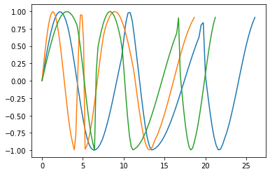
(b) Few functions from the first class.

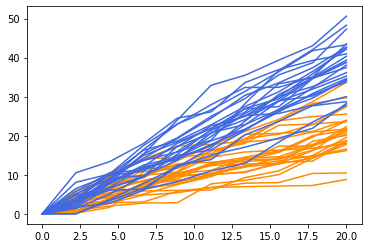
(c) Subset of warping functions colored by classes.

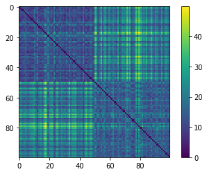
(d) Pairwise distances with dendrograms.

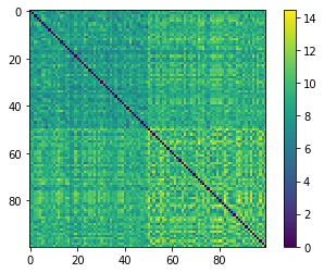
(e) Pairwise distances with $L_{2}$ metric.

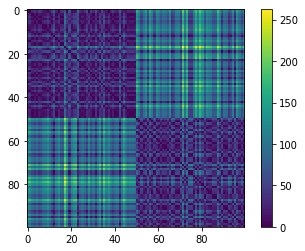
(f) Pairwise distances with $L_{2}$ metric on warping functions.

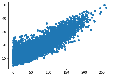
(g) Correlation between dendrograms and warping functions metric.

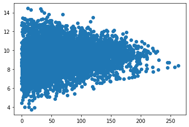
(h) Correlation between naive $L_{2}$ and warping functions metric.

Figure 13: Overview of the example of Section D.3.

The groups are discriminated by the parameters of the Gaussian distribution from which we sample the positive values $v_{i}$ to set up the warpings. For the first class we sample $N=10$ positive numbers from a truncated Gaussian with mean $3$ and standard deviation $2$; for the second the mean of the Gaussian is $5$ and the standard deviation is $2$. Thus we obtain each of the first $50$ functions sampling $10$ values $v_{i}$ from the truncated Gaussian centered in $3$, building the warping function as explained in the previous lines, and then reparametrizing the sine function accordingly. The following $50$ functions are obtained with the same pipeline but employing a Gaussian centered in $5$. Note that, by construction, all the functions in the data set share the same merge tree. We truncate the functions induced by $\Theta_{\mathcal{L}}$ at height $1$.

Examples of the warping functions can be seen in Figure 13(c); the resulting functions can be seen in Figure 13(a). The key point here is that we want to see if the dendrograms can retrieve the information contained in the warping functions. For this reason we compare the $L_{2}$ pairwise distances between such functions (see Figure 13(f)) and the pairwise distances obtained with dendrograms (see Figure 13(d)). The visual inspection confirms the close relationships between the two sources of information. Moreover, if we vectorize the arrays given by the two matrices (considering only entries above the diagonal) and compute the Fisher correlation, we get a score of $0.85$ (see Figure 13(g)). Instead, a naive approach with the $L_{2}$ metric applied directly to the data set would capture no information at all, as we can observe from Figure 13(e) and the Fisher correlation with the matrix obtained from warping functions is $0.15$ (see Figure 13(h)).

Note that, in general, the problem of finding warping functions to align functional data is deeply studied and with no easy solution (see, for instance, the special issue of the Electronic Journal of Statistics dedicated to phase and amplitude variability - year 2014, volume 8 or Srivastava et al. (2011)) especially for non-linear warping of multidimensional or non-euclidean domains. Instead, dendrograms less sensitive to such dimensionality issues, in the sense that they only arise in calculating the connected components and measure of the sublevel sets.

E Proofs

Proof of 3. Let $\pi_{0}(X_{\operatorname*{\scalerel*{\cdot}{\bigodot}}})$ be an abstract merge tree with critical values $t_{1}<\ldots<t_{n}$. Suppose that at $t_{j}$ changes happen across the critical value. Then we can fix $\varepsilon>0$ such that $t_{j}+\varepsilon<t_{j+1}$ and define $X_{\operatorname*{\scalerel*{\cdot}{\bigodot}}}^{\prime}$ with $X^{\prime}_{t}=X_{t}$ for all $t\neq t_{j}$ and $X^{\prime}_{t_{j}}=X_{t_{j}+\varepsilon}$. Now we need to define the $X_{\operatorname*{\scalerel*{\cdot}{\bigodot}}}^{\prime}$ on maps:

• if $t=t_{j}$ and $t<t^{\prime}\leq t_{j}+\varepsilon$, $X_{t<t^{\prime}}^{\prime}=(X_{t^{\prime}\leq t_{j}+\varepsilon})^{-1}$ which is well defined as $X_{t^{\prime}\leq t_{j}+\varepsilon}$ is an isomorphism;

• if $t^{\prime}=t_{j}$, $X_{t<t^{\prime}}^{\prime}=X_{t\leq t_{j}+\varepsilon}$ which is well defined as $X_{t^{\prime}\leq t_{j}+\varepsilon}$ is an isomorphism;

• otherwise $X^{\prime}_{t<t^{\prime}}=X_{t<t^{\prime}}$.

We need to check that $X_{\operatorname*{\scalerel*{\cdot}{\bigodot}}}^{\prime}$ is a regular abstract merge tree. First we have:

$$X^{\prime}_{t,t_{j}}\circ X^{\prime}_{t_{j},t^{\prime}}=X_{t\leq t_{j}+\varepsilon}\circ(X_{t^{\prime}\leq t_{j}+\varepsilon})^{-1}=X_{t,t^{\prime}}=X_{t,t^{\prime}}^{\prime}$$

if $t^{\prime}\leq t_{j}+\varepsilon$, otherwise

$$X^{\prime}_{t,t_{j}}\circ X^{\prime}_{t_{j},t^{\prime}}=X_{t\leq t_{j}+\varepsilon}\circ X_{t_{j}+\varepsilon\leq t^{\prime}}=X_{t,t^{\prime}}=X_{t,t^{\prime}}^{\prime}.$$

The filtration $X_{\operatorname*{\scalerel*{\cdot}{\bigodot}}}^{\prime}$ is regular at $t_{j}$ by construction as $X^{\prime}_{t_{j}}=X_{t_{j}+\varepsilon}\cong X^{\prime}_{t^{\prime}}$ for $t^{\prime}\in[t_{j},t_{j}+\varepsilon]$. Always by construction, it is a.e. isomorphic to $X_{\operatorname*{\scalerel*{\cdot}{\bigodot}}}$: the natural transformation $\varphi:X_{\operatorname*{\scalerel*{\cdot}{\bigodot}}}\rightarrow X_{\operatorname*{\scalerel*{\cdot}{\bigodot}}}^{\prime}$ is given by $\varphi_{t}=Id:X_{t}\rightarrow X^{\prime}_{t}$ for $t\neq t_{j}$ and, in fact, it is defined on $\mathbb{R}-\{t_{1},\ldots,t_{n}\}$.

If $t_{j}$ is the only critical value at which changes in $X_{\operatorname*{\scalerel*{\cdot}{\bigodot}}}$ happen across the value we are done, otherwise consider $t_{k}$ such that changes in $X_{\operatorname*{\scalerel*{\cdot}{\bigodot}}}$ happen across $t_{k}$. The same, by construction, holds also for $X_{\operatorname*{\scalerel*{\cdot}{\bigodot}}}^{\prime}$. Thus we can recursively apply the steps proposed up to now on $X_{\operatorname*{\scalerel*{\cdot}{\bigodot}}}^{\prime}$ until we obtain an abstract merge tree $R(\pi_{0}(X_{\operatorname*{\scalerel*{\cdot}{\bigodot}}}))$ which is regular. This is reached in a finite number of steps since the critical values are a finite set.

Uniqueness (up to isomorphism) follows easily.

$\blacksquare$

Proof of 4.

1. WLOG suppose $\pi_{0}(X_{\operatorname*{\scalerel*{\cdot}{\bigodot}}})\cong R(\pi_{0}(X_{\operatorname*{\scalerel*{\cdot}{\bigodot}}}))$; we build the merge tree $\mathcal{M}(\pi_{0}(X_{\operatorname*{\scalerel*{\cdot}{\bigodot}}}))=(T,h_{T})$ along the following rules in a recursive fashion starting from an empty set of vertices $V_{T}$ and an empty set of edges $E_{T}$. We simultaneously add points and edges to $T$ and define $h_{T}$ on the newly added vertices. Let $\{t_{i}\}_{i=1}^{n}$ be the critical set of $\pi_{0}(X_{\operatorname*{\scalerel*{\cdot}{\bigodot}}})$ and let $\pi_{0}(X_{t}):=a_{t}:=\{a^{t}_{1},\ldots,a^{t}_{n_{t}}\}$. Call $\psi_{t}^{t^{\prime}}:=\pi_{0}(X_{t\leq t^{\prime}})$. Lastly, from now on, we indicate with $\#C$ the cardinality of a finite set $C.$

   Considering in increasing order the critical values:

   • for the critical value $t_{1}$ add to $V_{T}$ a leaf $a_{t_{1}}^{k}$, with height $t_{1}$, for every element $a_{t_{1}}^{k}\in a_{t_{1}}$;

   • for $t_{i}$ with $i>1$, for every $a_{t_{i}}^{k}\in a_{t_{i}}$ such that $a_{t_{i}}^{k}\notin\text{Im}(\psi_{t_{i-1}}^{t_{i}}))$, add to $V_{T}$ a leaf $a_{t_{i}}^{k}$ with height $t_{i}$;

   • for $t_{i}$ with $i>1$, if $a_{t_{i}}^{k}=\psi_{t_{i-1}}^{t_{i}}(a_{t_{i-1}}^{s})=\psi_{t_{i-1}}^{t_{i}}(a_{t_{i-1}}^{r})$, with $a_{t_{i-1}}^{s}$ and $a_{t_{i-1}}^{r}$ distinct basis elements in $a_{t_{i-1}}$, add a vertex $a_{t_{i}}^{k}$ with height $t_{i}$, and add edges so that the previously added vertices

     $$v=\arg\max\{h_{T}(v^{\prime})\mid v^{\prime}\in V_{T}\text{ s.t. }\psi_{t_{v^{\prime}}}^{t_{i}}(v^{\prime})=a_{t_{i}}^{k}\}$$

     and

     $$w=\arg\max\{h_{T}(w^{\prime})\mid w^{\prime}\in V_{T}\text{ s.t. }\psi_{t_{w^{\prime}}}^{t_{i}}(w^{\prime})=a_{t_{i}}^{k}\}$$

     connect with the newly added vertex $a_{t_{i}}^{k}$.

   The last merging happens at height $t_{n}$ and, by construction, at height $t_{n}$ there is only one point, which is the root of the tree structure.

   These rules define a tree structure with a monotone increasing height function $h_{T}$. In fact, edges are induced by maps $\psi_{t}^{t^{\prime}}$ with $t<t^{\prime}$ and thus we can have no cycles and the function $h_{T}$ must be increasing. Moreover, we have $\psi_{t}^{t_{n}}(a_{i}^{t})=a_{1}^{t_{n}}$ for every $i$ and $t<t_{n}$ and thus the graph is path connected.

2. Now we start from a merge tree $(T,h_{T})$ and build an abstract merge tree $\pi_{0}(X_{\operatorname*{\scalerel*{\cdot}{\bigodot}}})$ such that $\mathcal{M}(\pi_{0}(X_{\operatorname*{\scalerel*{\cdot}{\bigodot}}}))\cong(T,h_{T})$.

   To build the abstract merge tree, the idea is that we would like to “cut” $(T,h_{T})$ at every height $t$ and take as many elements in the set of path connected components as the edges met by the cut.

   Let $\{t_{1},\ldots,t_{n}\}$ be the ordered image of $h_{T}$ in $\mathbb{R}$.

   Then consider the sets $v_{t_{j}}=\{v_{i}^{t_{j}}\}_{i=1,\ldots,n_{t_{j}}}=h_{T}^{-1}(t_{j})$. We use the notation $\mathcal{F}((T,h_{T}))_{t}:=a_{t}:=\{a^{t}_{1},\ldots,a^{t}_{n_{t}}\}$. We define $a_{t_{1}}=v_{t_{1}}$. For every $\varepsilon>0$ such that $t_{1}-t_{0}>\varepsilon$, we set $a_{t_{1}+\varepsilon}=a_{t_{1}}$ and consequently $\psi_{t}^{t^{\prime}}=Id$ for every $[t,t^{\prime}]\subset[t_{1},t_{2})$. Now we build $a_{t_{2}}$ starting from $a_{t_{1}}$ and using $v_{t_{2}}$. We need to consider $v_{i}^{t_{2}}\in v_{t_{2}}$. There are two possibilities:

   • if $v_{i}^{t_{2}}$ is a leaf, then we add $v_{i}^{t_{2}}$ to $a_{t_{1}}$;

   • if $v_{i}^{t_{2}}$ is an internal vertex with $\#\text{child}(v_{i}^{t_{2}})>1$ - i.e. a merging point, we add $v_{i}^{t_{2}}$ to $a_{t_{1}}$ and then remove $\text{child}(v_{i}^{t_{2}})=\{v\in V_{T}\mid v\text{ is a children of }v_{i}^{t_{2}}\}$. Note that, by construction $\text{child}(v_{i}^{t_{2}})\subset a_{t_{1}}$ and by hypothesis $\#\text{child}(v_{i}^{t_{2}})>1$;

   • if $v_{i}^{t_{2}}$ is an internal vertex with $\#\text{child}(v_{i}^{t_{2}})=1$ - i.e. an order $2$ vertex, we don’t do anything.

   By doing these operations for every $v_{i}^{t_{2}}\in v_{1}$, we obtain $a_{t_{2}}$. The map $\psi_{t}^{t_{2}}$, for $t\in[t_{1},t_{2})$ is then defined by setting $\psi_{t}^{t_{2}}(a_{i}^{t_{1}})=v_{i}^{t_{2}}$ if $a_{i}^{t_{1}}\in\text{child}(v_{i}^{t_{2}})$ and $\psi_{t}^{t_{2}}(a_{i}^{t_{1}})=a_{i}^{t_{1}}$ otherwise. To define $a_{t}$ for $t>t_{2}$ we recursively repeat for every critical value $t_{i}$ (in increasing order) the steps of defining $a_{t_{i}+\varepsilon}$ equal to $a_{t_{i}}$ for small $\varepsilon>0$ and then adjusting (as explained above) $a_{t_{i}}$ according to the tree structure to obtain $a_{i+1}$ and $\psi_{t_{i}}^{t_{i+1}}$. When reaching $t_{n}$ we have $v_{t_{n}}=\{v^{t_{n}}_{1}\}$ and we set $a_{t}=v_{t_{n}}$ for every $t\geq t_{n}$.

   We call this persistent set $\mathcal{F}((T,h_{T}))$. Note that, by construction:

   • for every $v\in V_{T}$ we have $v\in a_{t}$ for $t\in[h_{T}(v),h_{T}(\text{father}(v))$;

   • $\mathcal{F}((T,h_{T}))$ is regular;

   • $\mathcal{F}((T,h_{T}))$ is independent from order $2$ vertices of $(T,h_{T})$;

   • $\mathcal{F}((T,h_{T}))$ is an abstract merge tree.

   Now we need to check that $(T^{\prime},h_{T^{\prime}})=\mathcal{M}(\mathcal{F}((T,h_{T})))\cong_{2}(T,h_{T})$. WLOG we suppose $(T,h_{T})$ is without order $2$ vertices and prove $(T^{\prime},h_{T^{\prime}})=\mathcal{M}(\mathcal{F}((T,h_{T})))\cong(T,h_{T})$. Let $\pi_{0}(X_{\operatorname*{\scalerel*{\cdot}{\bigodot}}})=\mathcal{F}((T,h_{T}))$.

   As before, for notational convenience, we set $a_{t}:=\pi_{0}(X_{t})$ and $\psi_{t}^{t^{\prime}}:=\pi_{0}(X_{t\leq t^{\prime}})$. By construction, $a_{t}\subset V_{T}$ for every $t$. Which implies $V_{T^{\prime}}\subset V_{T}$.

   Consider now $a_{t_{i}}$ with $t_{i}$ critical value. To build $\pi_{0}(X_{\operatorname*{\scalerel*{\cdot}{\bigodot}}})$ elements $a_{j}^{t_{i-1}},a_{k}^{t_{i-1}}\in a_{t_{i-1}}$ are replaced by $v$ in $a_{t_{i}}$ if and only if they merge with $v$ in the merge tree $(T,h_{T})$: $(a_{j}^{t_{i-1}},v),(a_{k}^{t_{i-1}},v)$, with $h_{T}(v)=t_{i}$. The maps $\psi_{t_{i}}^{t_{i}}:a_{t_{i-1}}\rightarrow a_{t_{i-1}}$ are defined accordingly to represent that merging mapping $a_{j}^{t_{i-1}}\mapsto v$ and $a_{k}^{t_{i-1}}\mapsto v$. So an element $v^{\prime}$ stays in $a_{t}$ until the edge $(v^{\prime},father(v^{\prime}))$ meets another edge in $(T,h_{T})$, and then is replaces by $father(v^{\prime})$. As a consequence, we have $a_{j}^{t_{i-1}},a_{k}^{t_{i-1}},v\in V_{T^{\prime}}$ and $(a_{j}^{t_{i-1}},v),(a_{k}^{t_{i-1}},v)\in E_{T^{\prime}}$.

   Since $(T,h_{T})$ has no order $2$ vertices then 1) $V_{T}=\bigcup_{i=1,\ldots,n}a_{t_{i}}$ 2) $V_{T}=V_{T^{\prime}}$ 3) $id:V_{T}\rightarrow V_{T^{\prime}}$ is an isomorphism of merge trees.

   Now we consider $\pi_{0}(X_{\operatorname*{\scalerel*{\cdot}{\bigodot}}})$ regular abstract merge tree and prove $\mathcal{F}(\mathcal{M}(R(\pi_{0}(X_{\operatorname*{\scalerel*{\cdot}{\bigodot}}})))\cong\pi_{0}(X_{\operatorname*{\scalerel*{\cdot}{\bigodot}}})$. Consider $t_{i}$ critical value, $\varepsilon>0$ such that $t_{i-1}<t_{i}-\varepsilon$ and let $v_{t_{i}}=\{v\in\pi_{0}(X_{t_{i}})\mid\#\pi_{0}(X_{t_{i}-\varepsilon<t_{i}})^{-1}(v)\neq 1\}$. By construction, $v_{t_{i}}\subset V_{T}$, for every $t_{i}$ critical value, with $(T,h_{T})=\mathcal{M}(R(\pi_{0}(X_{\operatorname*{\scalerel*{\cdot}{\bigodot}}}))$.

   For every $v\in\pi_{0}(X_{t})$, for any $t\in\mathbb{R}$ there is $v_{j}^{t_{i}}\in v_{t_{i}}$ for some $t_{i}$, such that $\pi_{0}(X_{t_{i}\leq t})(v_{j}^{t_{i}})=v$. Moreover the following element is well defined:

   $$s(v):=\max\{w\in v_{t_{i}},t_{i}\text{ critical value }\mid\pi_{0}(X_{t_{i}\leq t})(w)=v\}$$

   By construction we have $v=\pi_{0}(X_{t_{i}\leq t})(s(v))$.

   Let $\pi_{0}(Y_{\operatorname*{\scalerel*{\cdot}{\bigodot}}})=\mathcal{F}(\mathcal{M}(R(\pi_{0}(X_{\operatorname*{\scalerel*{\cdot}{\bigodot}}})))$. Define $\alpha_{t}:\pi_{0}(X_{t})\rightarrow\pi_{0}(Y_{t})$ given by $v=\pi_{0}(X_{t_{i}\leq t})(s(v))\mapsto s(v)$. It is an isomorphism of abstract merge trees.

3. if $\pi_{0}(X_{\operatorname*{\scalerel*{\cdot}{\bigodot}}})\cong_{a.e.}\pi_{0}(Y_{\operatorname*{\scalerel*{\cdot}{\bigodot}}})$, then $R(\pi_{0}(X_{\operatorname*{\scalerel*{\cdot}{\bigodot}}}))\cong R(\pi_{0}(Y_{\operatorname*{\scalerel*{\cdot}{\bigodot}}}))$ and then the merge trees $\mathcal{M}(R(\pi_{0}(X_{\operatorname*{\scalerel*{\cdot}{\bigodot}}}))$ and $\mathcal{M}(R(\pi_{0}(Y_{\operatorname*{\scalerel*{\cdot}{\bigodot}}}))$ differ just by a change in the names of the vertices. If $\mathcal{M}(R(\pi_{0}(X_{\operatorname*{\scalerel*{\cdot}{\bigodot}}}))\cong\mathcal{M}(R(\pi_{0}(Y_{\operatorname*{\scalerel*{\cdot}{\bigodot}}}))$ then $\mathcal{F}(\mathcal{M}(R(\pi_{0}(X_{\operatorname*{\scalerel*{\cdot}{\bigodot}}})))\cong\mathcal{F}(\mathcal{M}(R(\pi_{0}(Y_{\operatorname*{\scalerel*{\cdot}{\bigodot}}})))\cong R(\pi_{0}(X_{\operatorname*{\scalerel*{\cdot}{\bigodot}}}))\cong R(\pi_{0}(Y_{\operatorname*{\scalerel*{\cdot}{\bigodot}}}))$.

4. the proof is analogous to the one of the previous point, with regularity condition on abstract merge trees being replaced by being without order $2$ vertices for merge trees.

$\blacksquare$

Proof of 6.

First note that even if $\inf\operatorname*{CA}(Q)$, with $Q\subset D_{\pi_{0}(X_{\operatorname*{\scalerel*{\cdot}{\bigodot}}})}$ and $\sup h(Q)<\infty$, may be a set with more than one element, $\inf\{h(p)\text{ with }p\in D_{\pi_{0}(X_{\operatorname*{\scalerel*{\cdot}{\bigodot}}})}\mid p\geq Q\}$ is uniquely defined. Moreover, consider $p=(b,t_{b}),q=(c,t_{c})\in\inf\operatorname*{CA}(Q)$. For every $(a,t)\in\operatorname*{CA}(Q)$ we know $\pi_{0}(X_{t_{b}\leq t})(b)=\pi_{0}(X_{t_{c}\leq t})(c)=a$. Clearly $t_{b}$ and $t_{c}$ must be critical values otherwise we can consider $p^{\prime}>p$ and $q^{\prime}>q$ with $q^{\prime},p^{\prime}\leq Q$, which is absurd. But the same holds if $t_{b}\neq t_{c}$: suppose $t_{b}<t_{c}\leq h(Q)$ then $p^{\prime}=(\pi_{0}(X_{t_{b}<t_{b}+\varepsilon})(b),t_{b}+\varepsilon)$ (with $\varepsilon>0$ small enough) satisfies $p<p^{\prime}$ and $p^{\prime}\leq Q$, which is absurd. Thus $t_{b}=t_{c}=t_{i}$ critical value.

The map $d:D_{\pi_{0}(X_{\operatorname*{\scalerel*{\cdot}{\bigodot}}})}\times D_{\pi_{0}(X_{\operatorname*{\scalerel*{\cdot}{\bigodot}}})}\rightarrow\mathbb{R}_{\geq 0}$ is symmetric. For what have said before $d(p,q)=0$ if and only if $p,q\in\inf\operatorname*{CA}(\{p,q\})$ and $h(p)=h(q)=t_{i}$ critical value. This is equivalent to $p=(b,t_{i}),q=(c,t_{i})\in D_{\pi_{0}(X_{\operatorname*{\scalerel*{\cdot}{\bigodot}}})}$ such that $\pi_{0}(X_{t_{i}<t_{i}+\varepsilon})(b)=\pi_{0}(X_{t_{i}<t_{i}+\varepsilon})(c)$ for every $\varepsilon>0$.

Thus, if $\pi_{0}(X_{\operatorname*{\scalerel*{\cdot}{\bigodot}}})$ is regular we have $d((b,t_{i}),(c,t_{i}))=0$ if and only if $p=q$; in fact $X_{t_{i}<t_{i}+\varepsilon}$ is an isomorphism for $\varepsilon>0$ small enough.

Now we check the triangle inequality. Let $p_{1},p_{2},p_{3}\in D_{\pi_{0}(X_{\operatorname*{\scalerel*{\cdot}{\bigodot}}})}$. And let $t_{i}=h(p_{i})$, $Q_{ij}=(p_{i},p_{j})$, $q_{ij}=\inf\{h(p)\text{ with }p\in\operatorname*{CA}(Q_{ij})\}$ and $q=\inf\{h(p)\text{ with }p\in\operatorname*{CA}(\{p_{1},p_{2},p_{3}\})\}$.

Consider $P_{1}=\operatorname*{CA}(\{p_{1}\})$. Clearly $\inf\operatorname*{CA}(\{p_{1},p_{2}\})\subset P_{1}$ and $\inf\operatorname*{CA}(\{p_{1},p_{3}\})\subset P_{1}$. Thus either (1) $q_{13}\leq q_{12}$ (and $q_{23}=q_{12}$) or (2) $q_{12}<q_{13}$ (and $q_{13}=q_{23}$) hold.

In case (1) holds:

$$q_{12}-t_{1}=q_{12}-q_{13}+q_{13}-t_{1}\leq q_{12}-q_{13}+q_{13}-t_{1}+2q_{13}-2t_{3}=q_{13}-t_{1}+q_{13}-t_{3}+q_{23}-t_{3}$$

Thus:

$$q_{12}-t_{1}+q_{12}-t_{2}\leq q_{13}-t_{1}+q_{13}-t_{3}+q_{23}-t_{3}+q_{23}-t_{2}$$

The proof in case (2) holds is analogous. $\blacksquare$

Proof of 10.

Let’s start with $\mathcal{O}\vee\mathcal{O}^{\prime}$. It is clearly an a.e. covering. Moreover $\bigcup_{U\in\mathcal{O}^{\prime}\text{ or }U\in\mathcal{O}}U$ is clearly contained in $\bigcup_{U\in\mathcal{U}(D_{\pi_{0}(X_{\operatorname*{\scalerel*{\cdot}{\bigodot}}})})}U$, and by functoriality we have that the set $\pi_{0}\left(\bigcup_{U\in\mathcal{O}^{\prime}\text{ or }U\in\mathcal{O}}U\right)$ is included in $\pi_{0}\left(\bigcup_{U\in\mathcal{U}(D_{\pi_{0}(X_{\operatorname*{\scalerel*{\cdot}{\bigodot}}})})}U\right).$ And the latter is equal to $\mathcal{U}(D_{\pi_{0}(X_{\operatorname*{\scalerel*{\cdot}{\bigodot}}})})$. Thus $\mathcal{O}\vee\mathcal{O}^{\prime}$ is regular and clearly is refined by $\mathcal{O}$ and $\mathcal{O}^{\prime}$. Lastly, consider any $\mathcal{O},\mathcal{O}^{\prime}<\mathcal{O}^{\prime\prime}$. Since the sets of $\mathcal{O}^{\prime\prime}$ are disjoint and path connected (by construction), then any $U^{\prime\prime}\in\mathcal{O}^{\prime\prime}$ contains all the sets of $\mathcal{O}$ and $\mathcal{O}^{\prime}$ it intersects. Thus it contains a path connected component of their union.

Now we turn to $\mathcal{O}\wedge\mathcal{O}^{\prime}$. All the sets in $\mathcal{O}\wedge\mathcal{O}^{\prime}$ are disjiont, open and path connected. And they form an a.e. cover of $D_{\pi_{0}(X_{\operatorname*{\scalerel*{\cdot}{\bigodot}}})}$ - otherwise a positive-measure set would be left out by $\mathcal{O}$ or $\mathcal{O}^{\prime}$. Thus $\mathcal{O}\wedge\mathcal{O}^{\prime}$ is a regular a.e. covering which refines $\mathcal{O}$ and $\mathcal{O}^{\prime}$. Consider $\mathcal{O}^{\prime\prime}$ such that $\mathcal{O},\mathcal{O}^{\prime}>\mathcal{O}^{\prime\prime}$. Take $U^{\prime\prime}\in\mathcal{O}^{\prime\prime}$. By construction there are $U\in\mathcal{O}$ and $U^{\prime}\in\mathcal{O}^{\prime}$ with $U^{\prime\prime}\subset U^{\prime},U$. Thus $U^{\prime\prime}\subset U\cap U^{\prime}$. So $\mathcal{O}^{\prime\prime}<\mathcal{O}\wedge\mathcal{O}^{\prime}$.

$\blacksquare$

Proof of 2.

The proof is largely based on Theorem 1 in Pegoraro and Secchi (2021).

First notice that $\parallel\varphi_{T}^{\Theta_{1}}((v,v^{\prime}))\parallel_{L_{1}(\mathbb{R})}=h_{T}(v^{\prime})-h_{T}(v)=w_{T}((v,v^{\prime}))$ - see LABEL:sec:positive_editable. Thus the cost of deleting $v$ in $(T,w_{T})$ is the same as in $(T,\varphi_{T}^{\Theta_{1}})$.

Second, consider the following cases:

1. if $h_{T}(v)<h_{T^{\prime}}(w)<h_{T}(v^{\prime})<h_{T^{\prime}}(w^{\prime})$:

   $$\parallel\varphi_{T}^{\Theta_{1}}((v,v^{\prime}))-\varphi_{T^{\prime}}^{\Theta_{1}}((w,w^{\prime}))\parallel_{L_{1}(\mathbb{R})}=\mid h_{T}(v)+h_{T}(w)-h_{T^{\prime}}(w)-h_{T^{\prime}}(w^{\prime})\mid;$$

2. if $h_{T}(v)<h_{T}(v^{\prime})<h_{T^{\prime}}(w)<h_{T^{\prime}}(w^{\prime})$:

   $$\parallel\varphi_{T}^{\Theta_{1}}((v,v^{\prime}))-\varphi_{T^{\prime}}^{\Theta_{1}}((w,w^{\prime}))\parallel_{L_{1}(\mathbb{R})}=w_{T}((v,v^{\prime}))+w_{T^{\prime}}((w,w^{\prime}));$$

3. if $h_{T}(v)<h_{T^{\prime}}(w)<h_{T^{\prime}}(w^{\prime})<h_{T}(v^{\prime})$:

   $$\parallel\varphi_{T}^{\Theta_{1}}((v,v^{\prime}))-\varphi_{T^{\prime}}^{\Theta_{1}}((w,w^{\prime}))\parallel_{L_{1}(\mathbb{R})}=w_{T}((v,v^{\prime}))-w_{T^{\prime}}((w,w^{\prime})).$$

Consider the same mapping $M$ constructed in the proof of Theorem 1 in Pegoraro and Secchi (2021). As in 4 $M$ is such that:

• the deletions $(v,"D")$ and $("D",w)$ are always such that $w_{T^{\prime}}(w),w_{T}(v)\leq 2\varepsilon$;

• for any edge $(v,v^{\prime})$ which is shrink on $(w,w^{\prime})$ after all ghostings and deletions on $T$ and on $T^{\prime}$ we have $\mid h_{T}(v)-h_{T^{\prime}}(w)\mid<\varepsilon$ and $\mid h_{T}(v^{\prime})-h_{T^{\prime}}(w^{\prime})\mid<2\varepsilon$.

As a consequence:

1. if $h_{T}(v)<h_{T^{\prime}}(w)<h_{T}(v^{\prime})<h_{T^{\prime}}(w^{\prime})$: $cost_{M}((v,w))\leq 2\varepsilon$;

2. if $h_{T}(v)<h_{T}(v^{\prime})<h_{T^{\prime}}(w)<h_{T^{\prime}}(w^{\prime})$: since $h_{T^{\prime}}(w)-h_{T}(v)<\varepsilon$, then $w_{T}((v,v^{\prime})),w_{T^{\prime}}((w,w^{\prime}))<\varepsilon$. So $cost_{M}((v,w))\leq 2\varepsilon$.

3. if $h_{T}(v)<h_{T^{\prime}}(w)<h_{T^{\prime}}(w^{\prime})<h_{T}(v^{\prime})$: $cost_{M}((v,w))\leq 2\varepsilon$.

$\blacksquare$

References

- Adams et al. (2017) H. Adams, Tegan Emerson, M. Kirby, R. Neville, C. Peterson, P. Shipman, Sofya Chepushtanova, E. Hanson, F. Motta, and Lori Ziegelmeier. Persistence images: A stable vector representation of persistent homology. Journal of Machine Learning Research, 18(1):1–35, 2017.
- Audin et al. (2014) Michele Audin, Mihai Damian, and Reinie Erné. Morse theory and Floer homology. Springer, 2014.
- Bauer et al. (2014) Ulrich Bauer, Elizabeth Munch, and Yusu Wang. Strong equivalence of the interleaving and functional distortion metrics for reeb graphs. arXiv, 2014.
- Bauer et al. (2020) Ulrich Bauer, Claudia Landi, and Facundo Mémoli. The reeb graph edit distance is universal. Foundations of Computational Mathematics, pages 1–24, 2020.
- Beketayev et al. (2014) Kenes Beketayev, Damir Yeliussizov, Dmitriy Morozov, Gunther H. Weber, and Bernd Hamann. Measuring the distance between merge trees. In Topological Methods in Data Analysis and Visualization, pages 151–166. Springer International Publishing, Cham, 2014.
- Bhattacharya et al. (2015) Subhrajit Bhattacharya, Robert Ghrist, and Vijay Kumar. Persistent homology for path planning in uncertain environments. IEEE Transactions on Robotics, 31:1–13, 2015.
- Biasotti et al. (2008) Silvia Biasotti, Daniela Giorgi, Michela Spagnuolo, and Bianca Falcidieno. Reeb graphs for shape analysis and applications. Theoretical Computer Science, 392(1-3):5–22, 2008.
- Bille (2005) Philip Bille. A survey on tree edit distance and related problems. Theoretical Computer Science, 337(1-3):217 – 239, 2005.
- Billera et al. (2001) Louis J Billera, Susan P Holmes, and Karen Vogtmann. Geometry of the space of phylogenetic trees. Advances in Applied Mathematics, 27(4):733–767, 2001.
- Bock et al. (2017) Alexander Bock, Harish Doraiswamy, Adam Summers, and Claudio Silva. Topoangler: Interactive topology-based extraction of fishes. IEEE Transactions on Visualization and Computer Graphics, 2017.
- Bubenik (2015) Peter Bubenik. Statistical topological data analysis using persistence landscapes. Journal of Machine Learning Research, 16(3):77–102, 2015.
- Burago et al. (2022) Dmitri Burago, Yuri Burago, and Sergei Ivanov. A course in metric geometry, volume 33. American Mathematical Society, 2022.
- Cardona et al. (2021) Robert Cardona, Justin Curry, Tung Lam, and Michael Lesnick. The universal -metric on merge trees. arXiv, 2112.12165 [cs.CG], 2021.
- Carlsson and Mémoli (2013) Gunnar Carlsson and Facundo Mémoli. Classifying clustering schemes. Foundations of Computational Mathematics, 13, 2013.
- Carstens and Horadam (2013) Corrie Jacobien Carstens and Kathy Horadam. Persistent homology of collaboration networks. Mathematical Problems in Engineering, 2013, 2013.
- Chazal et al. (2015) F. Chazal, Brittany Terese Fasy, F. Lecci, A. Rinaldo, and L. Wasserman. Stochastic convergence of persistence landscapes and silhouettes. Journal of Computational Geometry, 6(2):140–161, 2015.
- Chazal et al. (2016) Frédéric Chazal, Vin De Silva, Marc Glisse, and Steve Oudot. The structure and stability of persistence modules. Springer, 2016.
- Chazal et al. (2008) Frédéric Chazal, David Cohen-Steiner, Marc Glisse, Leonidas Guibas, and Steve Oudot. Proximity of persistence modules and their diagrams. Proc. 25th ACM Sympos. Comput. Geom., 12 2008.
- Cohen-Steiner et al. (2007) D. Cohen-Steiner, H. Edelsbrunner, and J. Harer. Stability of persistence diagrams. Discrete & Computational Geometry, 37:103–120, 2007.
- Cohen-Steiner et al. (2010) David Cohen-Steiner, Herbert Edelsbrunner, John Harer, and Yuriy Mileyko. Lipschitz functions have lp-stable persistence. Foundations of Computational Mathematics, 10:127–139, 2010.
- Curry (2018) Justin Curry. The fiber of the persistence map for functions on the interval. Journal of Applied and Computational Topology, 2, 2018.
- Curry et al. (2021) Justin Curry, Jordan DeSha, Adélie Garin, Kathryn Hess, Lida Kanari, and Brendan Mallery. From trees to barcodes and back again ii: Combinatorial and probabilistic aspects of a topological inverse problem. arXiv, 2107.11212, 2021.
- Curry et al. (2022) Justin Curry, Haibin Hang, Washington Mio, Tom Needham, and Osman Berat Okutan. Decorated merge trees for persistent topology. Journal of Applied and Computational Topology, 2022.
- De Silva et al. (2016) Vin De Silva, Elizabeth Munch, and Amit Patel. Categorified reeb graphs. Discrete & Computational Geometry, 55(4):854–906, 2016.
- Di Fabio and Landi (2016) Barbara Di Fabio and Claudia Landi. The edit distance for reeb graphs of surfaces. Discrete & Computational Geometry, 55(2):423–461, 2016.
- Dryden and Mardia (1998) I. L. Dryden and K. V. Mardia. Statistical Shape Analysis. Wiley, Chichester, 1998.
- Edelsbrunner et al. (2002) H. Edelsbrunner, D. Letscher, and A. Zomorodian. Topological persistence and simplification. Discrete & Computational Geometry, 28:511–533, 2002.
- Edelsbrunner and Harer (2008) Herbert Edelsbrunner and John Harer. Persistent homology—a survey. In Surveys on discrete and computational geometry, volume 453 of Contemporary Mathematics, pages 257–282. American Mathematical Society, Providence, RI, 2008.
- Elkin and Kurlin (2021) Yury Elkin and Vitaliy Kurlin. Isometry invariant shape recognition of projectively perturbed point clouds by the mergegram extending 0d persistence. Mathematics, 9(17), 2021.
- Emmett et al. (2015) K. Emmett, Benjamin Schweinhart, and R. Rabadan. Multiscale topology of chromatin folding. In Proceedings of the 9th EAI International Conference on Bio-inspired Information and Communications Technologies, 2015.
- Fasy et al. (2014) Brittany Fasy, Fabrizio Lecci, Alessandro Rinaldo, Larry Wasserman, Sivaraman Balakrishnan, and Aarti Singh. Confidence sets for persistence diagrams. The Annals of Statistics, 42:2301–2339, 2014.
- Felsenstein and Felenstein (2004) Joseph Felsenstein and Joseph Felenstein. Inferring phylogenies, volume 2. Sinauer associates Sunderland, MA, 2004.
- Feragen et al. (2012) Aasa Feragen, Pechin Lo, Marleen de Bruijne, Mads Nielsen, and Francois Lauze. Toward a theory of statistical tree-shape analysis. IEEE Transactions on Pattern Analysis and Machine Intelligence, 2012.
- Gameiro et al. (2014) Marcio Gameiro, Yasuaki Hiraoka, Shunsuke Izumi, Miroslav Kramár, Konstantin Mischaikow, and Vidit Nanda. A topological measurement of protein compressibility. Japan Journal of Industrial and Applied Mathematics, 32:1–17, 2014.
- Gao et al. (2010) Xinbo Gao, Bing Xiao, Dacheng Tao, and Xuelong Li. A survey of graph edit distance. Pattern Analysis and applications, 13:113–129, 2010.
- Garba et al. (2021) Maryam Kashia Garba, Tom MW Nye, Jonas Lueg, and Stephan F Huckemann. Information geometry for phylogenetic trees. Journal of Mathematical Biology, 82(3):1–39, 2021.
- Gasparovic et al. (2019) Ellen Gasparovic, E. Munch, S. Oudot, Katharine Turner, B. Wang, and Yusu Wang. Intrinsic interleaving distance for merge trees. ArXiv, 1908.00063v1[cs.CG], 2019.
- Giusti et al. (2016) Chad Giusti, Robert Ghrist, and Danielle Bassett. Two’s company, three (or more) is a simplex: Algebraic-topological tools for understanding higher-order structure in neural data. Journal of Computational Neuroscience, 41, 2016.
- Hatcher (2000) Allen Hatcher. Algebraic topology. Cambridge University Press, Cambrige, 2000.
- Hein et al. (1995) Jotun Hein, Tao Jiang, Lusheng Wang, and Kaizhong Zhang. On the complexity of comparing evolutionary trees. In Combinatorial Pattern Matching, pages 177–190, Berlin, Heidelberg, 1995. Springer Berlin Heidelberg.
- Hofer et al. (2017) C. Hofer, R. Kwitt, M. Niethammer, and A. Uhl. Deep learning with topological signatures. In NIPS, 2017.
- Hong et al. (2017) Eunpyeong Hong, Yasuaki Kobayashi, and Akihiro Yamamoto. Improved methods for computing distances between unordered trees using integer programming. In International Conference on Combinatorial Optimization and Applications, pages 45–60. Springer, 2017.
- Kanari et al. (2020) Lida Kanari, Adélie Garin, and Kathryn Hess. From trees to barcodes and back again: theoretical and statistical perspectives. ArXiv, 2010.11620[math.AT], 2020.
- Kendall (1977) D. G. Kendall. The diffusion of shape. Advances in Applied Probability, 1977.
- Kendall (1984) D. G. Kendall. Shape Manifolds, Procrustean Metrics, and Complex Projective Spaces. Bulletin of the London Mathematical Society, 1984.
- Kovacev-Nikolic et al. (2016) Violeta Kovacev-Nikolic, Peter Bubenik, Dragan Nikolic, and Giseon Heo. Using persistent homology and dynamical distances to analyze protein binding. Statistical applications in genetics and molecular biology, 15:19–38, 2016.
- Kramár et al. (2013) Miroslav Kramár, Arnaud Goullet, Lou Kondic, and K Mischaikow. Persistence of force networks in compressed granular media. Physical review. E, Statistical, nonlinear, and soft matter physics, 87, 2013.
- Lacombe et al. (2018) T. Lacombe, Marco Cuturi, and S. Oudot. Large scale computation of means and clusters for persistence diagrams using optimal transport. In NeurIPS, 2018.
- Lord et al. (2016) Louis-David Lord, Paul Expert, Henrique Fernandes, Giovanni Petri, Tim Van Hartevelt, Francesco Vaccarino, Gustavo Deco, Federico Turkheimer, and Morten Kringelbach. Insights into brain architectures from the homological scaffolds of functional connectivity networks. Frontiers in Systems Neuroscience, 10:85, 2016.
- Lum et al. (2013) P. Y. Lum, G. Singh, A. Lehman, T. Ishkanov, M. Alagappan, J. Carlsson, G. Carlsson, and Mikael Vilhelm Vejdemo Johansson. Extracting insights from the shape of complex data using topology. Scientific Reports, 3, 2013.
- MacPherson and Schweinhart (2010) Robert MacPherson and Benjamin Schweinhart. Measuring shape with topology. Journal of Mathematical Physics, 53, 2010.
- Maletić et al. (2015) Slobodan Maletić, Yi Zhao, and Milan Rajkovic. Persistent topological features of dynamical systems. Chaos: An Interdisciplinary Journal of Nonlinear Science, 26, 2015.
- Mileyko et al. (2011) Yuriy Mileyko, Sayan Mukherjee, and John Harer. Probability measures on the space of persistence diagrams. Inverse Problems, 27, 2011.
- Morozov et al. (2013) Dmitriy Morozov, Kenes Beketayev, and Gunther Weber. Interleaving distance between merge trees. Discrete & Computational Geometry, 49:22–45, 2013.
- Murtagh and Contreras (2017) Fionn Murtagh and Pedro Contreras. Algorithms for hierarchical clustering: An overview, ii. Wiley Interdisciplinary Reviews: Data Mining and Knowledge Discovery, 7(6):e1219, 2017.
- Naitzat et al. (2020) Gregory Naitzat, Andrey Zhitnikov, and Lek-Heng Lim. Topology of deep neural networks. Journal of Machine Learning Research, 21(184):1–40, 2020.
- Pascucci and Cole-McLaughlin (2003) Valerio Pascucci and Kree Cole-McLaughlin. Parallel computation of the topology of level sets. Algorithmica, 38:249–268, 2003.
- Patel (2018) Amit Patel. Generalized persistence diagrams. Journal of Applied and Computational Topology, 1, 2018.
- Pegoraro (2021a) Matteo Pegoraro. A locally stable stable edit distance for merge trees. arXiv, 2111.02738 [math.GN], 2021a.
- Pegoraro (2021b) Matteo Pegoraro. A combinatorial approach to interleaving distance between merge trees. arXiv, 2111.15531[math.co], 2021b.
- Pegoraro (2023) Matteo Pegoraro. A persistence-driven edit distance for graphs with abstract weights. arXiv, 2304.12088 [math.CO], 2023.
- Pegoraro and Secchi (2021) Matteo Pegoraro and Piercesare Secchi. Functional data representation with merge trees. arXiv, 2108.13147v2 [stat.ME], 2021.
- Perea and Harer (2013) Jose Perea and John Harer. Sliding windows and persistence: An application of topological methods to signal analysis. Foundations of Computational Mathematics, 15, 2013.
- Perea et al. (2015) Jose Perea, Anastasia Deckard, Steven Haase, and John Harer. Sw1pers: Sliding windows and 1-persistence scoring; discovering periodicity in gene expression time series data. BMC bioinformatics, 16:257, 2015.
- Pokorny et al. (2015) Florian Pokorny, Majd Hawasly, and Subramanian Ramamoorthy. Topological trajectory classification with filtrations of simplicial complexes and persistent homology. The International Journal of Robotics Research, 35, 2015.
- Rizvi et al. (2017) Abbas Rizvi, Pablo Camara, Elena Kandror, Thomas Roberts, Ira Schieren, Tom Maniatis, and Raul Rabadan. Single-cell topological rna-seq analysis reveals insights into cellular differentiation and development. Nature Biotechnology, 35, 2017.
- Sangalli et al. (2010) Laura Sangalli, Piercesare Secchi, Simone Vantini, and Valeria Vitelli. K-mean alignment for curve clustering. Computational Statistics & Data Analysis, 54:1219–1233, 2010.
- Scolamiero et al. (2017) Martina Scolamiero, Wojciech Chachólski, Anders Lundman, Ryan Ramanujam, and Sebastian Öberg. Multidimensional persistence and noise. Foundations of Computational Mathematics, 17(6):1367–1406, 2017.
- Shinagawa et al. (1991) Y. Shinagawa, T. L. Kunii, and Y. L. Kergosien. Surface coding based on morse theory. IEEE Computer Graphics and Applications, 11(5):66–78, 1991.
- Silva and Ghrist (2007) Vin Silva and Robert Ghrist. Coverage in sensor networks via persistent homology. Algebraic & Geometric Topology, 7, 2007.
- Sizemore et al. (2015) Ann Sizemore, Chad Giusti, and Danielle Bassett. Classification of weighted networks through mesoscale homological features. Journal of Complex Networks, 5, 2015.
- Smith and Kurlin (2022) Philip Smith and Vitaliy Kurlin. Families of point sets with identical 1d persistence. arXiv, 2202.00577 [cs.CG], 2022.
- Sridharamurthy et al. (2020) R. Sridharamurthy, T. B. Masood, A. Kamakshidasan, and V. Natarajan. Edit distance between merge trees. IEEE Transactions on Visualization and Computer Graphics, 26(3):1518–1531, 2020.
- Srivastava et al. (2011) A. Srivastava, W. Wu, S. Kurtek, E. Klassen, and J. S. Marron. Registration of functional data using fisher-rao metric. arXiv, arXiv:1103.3817v2 [math.ST], 2011.
- Tai (1979) Kuo-Chung Tai. The tree-to-tree correction problem. Journal of the ACM, 26:422–433, 1979.
- Touli (2020) Elena Farahbakhsh Touli. Frechet-like distances between two merge trees. ArXiv, 2004.10747v1[cs.CC], 2020.
- Touli and Wang (2018) Elena Farahbakhsh Touli and Yusu Wang. Fpt-algorithms for computing gromov-hausdorff and interleaving distances between trees. In ESA, 2018.
- Turner et al. (2012) Katharine Turner, Yuriy Mileyko, Sayan Mukherjee, and John Harer. Frechet means for distributions of persistence diagrams. Discrete & Computational Geometry, 52, 06 2012.
- Wang and Marron (2007) Haonan Wang and J. S. Marron. Object oriented data analysis: Sets of trees. Annals of Statistics, 35(5):1849–1873, 2007.
- Wetzels et al. (2022) Florian Wetzels, Heike Leitte, and Christoph Garth. Branch decomposition-independent edit distances for merge trees. Comput. Graph. Forum, 41(3):367–378, 2022.
- wu and Zhang (2013) Keqin wu and Song Zhang. A contour tree based visualization for exploring data with uncertainty. International Journal for Uncertainty Quantification, 3:203–223, 2013.
- Xia et al. (2015) Kelin Xia, Xin Feng, Yiying Tong, and Guo We. Persistent homology for the quantitative prediction of fullerene stability. Journal of Computational Chemistry, 36, 2015.
- Xu and Tian (2015) Dongkuan Xu and Yingjie Tian. A comprehensive survey of clustering algorithms. Annals of Data Science, 2, 2015.
- Zomorodian and Carlsson (2005) Afra Zomorodian and Gunnar Carlsson. Computing persistent homology. Discrete & Computational Geometry, 33:249–274, 2005.