The diffuse interstellar band around 8620 Å

Abstract

Context. Diffuse interstellar bands (DIBs) are important interstellar absorption features of which the origin is still debated. With the large data sets from modern spectroscopic surveys, background stars are widely used to show how the integrated columns of DIB carriers accumulate from the Sun to great distances. To date, studies on the kinematics of the DIB carriers are still rare.

Aims. We aim to make use of the measurements from the Giraffe Inner Bulge Survey (GIBS) and the Gaia–ESO survey (GES) to study the kinematics and distance of the carrier of DIB $\lambda$8620, as well as other properties.

Methods. The DIBs were detected and measured following the same procedures as in Paper $\rm I$, assuming a Gaussian profile. The median radial velocities of the DIB carriers in 38 GIBS and GES fields were used to trace their kinematics, and the median distances of the carriers in each field were estimated by the median radial velocities and two applied Galactic rotation models.

Results. We successfully detected and measured DIB $\lambda$8620 in 760 of 4117 GES spectra with $|b|\,{\leqslant}\,10^{\circ}$ and $\rm S/N>50$. Combined with the DIBs measured in GIBS spectra (Paper $\rm I$), we confirmed a tight relation between EW and $E(J\,{-}\,K_{\rm S})$ as well as $A_{\rm V}$, with similar fitting coefficients to those found by previous works. With a more accurate sample and the consideration of the solar motion, the rest-frame wavelength of DIB $\lambda$8620 was redetermined as 8620.83 Å, with a mean fit error of 0.36 Å. We studied the kinematics of the DIB carriers by tracing their median radial velocities in each field in the local standard of rest ($V_{\rm LSR}$) and into the galactocentric frame ($V_{\rm GC}$), respectively, as a function of the Galactic longitudes. Based on the median $V_{\rm LSR}$ and two Galactic rotation models, we obtained valid kinematic distances of the DIB carriers for nine GIBS and ten GES fields. We also found a linear relation between the DIB $\lambda$8620 measured in this work and the near-infrared DIB in APOGEE spectra at $1.5273\,\rm\mu m$, and we estimated the carrier abundance to be slightly lower compared to the DIB $\lambda$15273.

Conclusions. We demonstrate that the DIB carriers can be located much closer to the observer than the background stars based on the following arguments: (i) qualitatively, the carriers occupy in the Galactic longitude–velocity diagram typical rotation velocities of stars in the local Galactic disk, while the background stars in the GIBS survey are mainly located in the Galactic bulge; (ii) quantitatively, all the derived kinematic distances of the DIB carriers are smaller than the median distances to background stars in each field. A linear correlation between DIB $\lambda$8620 and DIB $\lambda$15273 has been established, showing similar carrier abundances and making them both attractive for future studies of the interstellar environments.

1 Introduction

Diffuse interstellar bands (DIBs) are a set of absorption features that can be observed nearly everywhere in the spectra from optical to infrared wavelengths. DIBs were first observed in 1919 (Heger, 1922) and then named and definitively determined as interstellar features in the 1930s (Merrill & Wilson, 1938). Strong optical DIBs, such as the famous $\lambda$5780 and $\lambda$5797 (Heger, 1922) and $\lambda$6284 and $\lambda$6614 (Merrill, 1930), were discovered and studied first. Then, with the increase of spectral resolution, more and more DIBs, especially weak features, were reported. An example mentioned in Krełowski (2018), a recent review, was that in the spectral window 5700–5860 Å, Heger (1922) mentioned two DIBs, Herbig (1975) mentioned five, and after, with Hobbs et al. (2009), the number increased to 30. In the latest published catalog (Fan et al., 2019), this range contained 51 DIBs. Of course, most of them are very weak features that can only be detected in high-resolution, high signal-to-noise (S/N) spectra. DIBs were also discovered at infrared bands (e.g., Cox et al., 2014; Hamano et al., 2015; Galazutdinov et al., 2017a) and in distant galaxies (Monreal-Ibero et al., 2015, 2018).

The most important topic with regard to the DIBs is the identification of their carriers, which is usually described as “the longest-standing unsolved mystery in astronomical spectroscopy” (see Zack & Maier 2014, Tielens 2014, Geballe 2016, and Krełowski 2018 for recent reviews). Today, carbon-bearing molecules, such as carbon chains (Maier et al., 2004), polycyclic aromatic hydrocarbons (PAHs, Omont et al., 2019), and fullerenes (Omont, 2016), are thought to be the most likely candidates for the DIB carriers. As the direct comparison between the observations and the laboratory predictions is very difficult, buckminsterfullerene $(C_{60}^{+})$ is the first and only identified DIB carrier for five near-infrared (NIR) DIBs (Campbell et al., 2015; Walker et al., 2016; Campbell et al., 2016a, b; Cordiner et al., 2017; Walker et al., 2017; Campbell & Maier, 2018; Lallement et al., 2018; Cordiner et al., 2019; Linnartz et al., 2020), although some debates still exist (e.g., Galazutdinov et al., 2017b, 2021). Besides the laboratory investigations, modern spectroscopy also provides observational clues for the carrier research. Mutual correlations between different DIBs (e.g., McCall et al., 2010; Friedman et al., 2011; Elyajouri et al., 2017) facilitate the estimation of a single carrier for a set of DIBs, although it is still too early to conclude the same origin for any pair because of the variation of their strength ratio (Krełowski et al., 2016). Elyajouri et al. (2018) reported a tight correlation between the strength of the so-called $C_{2}$-DIBs (Thorburn et al., 2003) and the $C_{2}$ column density, which is very different from other non-$C_{2}$ DIBs. They also discovered substructures for at least 14 $C_{2}$-DIBs, which may reveal information about the rotational branches of the carriers. It should be noted that although dust grain lost its qualification as the carrier candidate (see e.g., Cox et al., 2007, 2011; Xiang et al., 2017), the tight correlation between the DIB strength and interstellar extinction for many strong DIBs (e.g., Lan et al., 2015) means that the DIB carriers are well mixed with the interstellar dust grains.

The studies related to the DIB carriers focus on their physical identifications, while very few works pay attention to the kinematics and distances of the DIB carriers. As the statistical research was not available during the early studies, which usually made use of only a few to tens of spectra, the unresolved carriers alleviate the importance and necessity of the kinematic study. However, kinematic research benefits from the large spectroscopic surveys and can reveal the rotation curve of the DIB carriers, such as the longitude–velocity diagram built for the NIR DIB $\lambda$15273 (Zasowski et al., 2015) based on the APOGEE spectra (Eisenstein et al., 2011). The three-dimensional (3D) distribution of the DIB carrier is revealed by modern spectroscopic surveys (e.g., Kos et al., 2014; Zasowski et al., 2015). Furthermore, DIBs are also proven to be good tracers of Galactic arms (Puspitarini et al., 2015; Puspitarini & Lallement, 2019). In this work, we aim to establish a kinematic study of the DIB $\lambda$8620 (although the rest-frame wavelength, $\lambda_{0}$, for this DIB is larger than 8620 Å, we still call it DIB $\lambda$8620 for brevity) and estimate the kinematic distance of its carrier.

The DIB $\lambda$8620 was first observed in the spectrum of the star HD 183143 (Geary, 1975) and then confirmed as an interstellar band by Sanner et al. (1978), who further reported $\lambda_{0}\,{=}\,8620.7\,{\pm}\,0.3$ Å and derived a linear correlation between the DIB strength and $E(B\,{-}\,V)$. Later on, various $\lambda_{0}$ were measured by different works: 8620.75 Å (Herbig & Leka, 1991), 8621.2 Å (Jenniskens & Desert, 1994), 8620.8 Å (Galazutdinov et al., 2000), and 8620.18 Å (Fan et al., 2019). In the new century, DIB $\lambda$8620 attracts more attention because it is within the spectral window of the RAdial Velocity Experiment (RAVE) survey (Steinmetz et al., 2006). A tight correlation with $E(B\,{-}\,V)$ was confirmed by Munari et al. (2008) using 68 hot stars from RAVE, and $\lambda_{0}=8620.4\pm 0.1$ Å was suggested. Moreover, Kos et al. (2013) and Kos et al. (2014) built the first pseudo-3D intensity map for DIB $\lambda$8620 using $\sim$500,000 RAVE spectra. The correlation between the DIB strength and interstellar extinction was also studied by Wallerstein et al. (2007), Puspitarini et al. (2015), and Damineli et al. (2016). Nearly all the linear coefficients derived by different works are slightly different from each other, but most of them still correspond with each other considering the uncertainties. Zhao et al. (2021, hereafter Paper I) developed a set of procedures for automatic detection and measurement of the DIB $\lambda$8620 in a spectral window between 8605 and 8640 Å. The DIB quantities, depth, width, central wavelength ($\lambda_{C}$), and equivalent width (EW), can be measured from the Gaussian profile, together with their uncertainties and the quality flag (QF), which evaluates the reliability of the fit. The procedures were tested with 4797 low-resolution spectra from the Giraffe Inner Bulge Survey (GIBS; Zoccali et al., 2014), a survey of red clump (RC) stars in the Galactic bulge. We derived the EW–$E(J\,{-}\,K_{\rm S})$ linear relation in three ways by the median quantities in reddening bins, in observational fields, and with a pure RC sample (see Table 1 and Sect 4.1 in Paper $\rm I$ for details). The recommended result was $E(J\,{-}\,K_{\rm S})\,{=}\,1.884\,({\pm}\,0.225)\,{\times}\,{\rm EW}\,{-}\,0.012\,({\pm}\,0.072)$, which was a medium value in comparison with other results and closest to Munari et al. (2008), under the conversion with a specific extinction law.

In this paper, we continue to study the kinematics and distance of the carrier of DIB $\lambda$8620, with high-quality results from the GIBS samples used in Paper $\rm I$ and new samples from the Gaia–ESO Spectroscopic Survey (GES; Gilmore et al., 2012). In Sect. 2, we describe the spectra used in this work and define the fields for further analysis. The linear relation between EW and extinction is derived and discussed in Sect. 3. Section 4 presents the kinematic studies of the DIB carriers. The estimation of the carrier distance is introduced and discussed in Sect. 5. In Sect. 6, a rough comparison between DIB $\lambda$8620 and DIB $\lambda$15273 is made to study their possible correlation. The main conclusions are summarized in Sect. 7.

2 Samples and fields

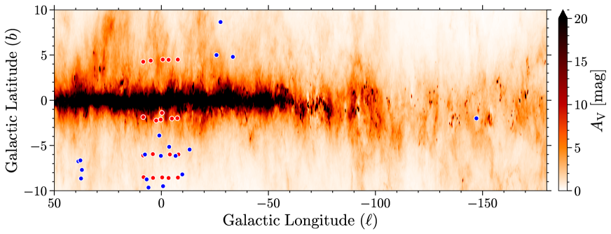
Figure 1: Locations of 20 GIBS observational fields (red dots) and 18 GES selected fields (blue dots), overplotted on the extinction map of Schlegel et al. (1998) calibrated by Schlafly & Finkbeiner (2011).

Giraffe Inner Bulge Survey (GIBS) is a dedicated survey to study the kinematics and chemistry of RC stars in the Galactic bulge (Zoccali et al., 2014). In Paper $\rm I$, we constructed a pure RC sample applying an additional criterion where we consider stars only to be on the RC if their $J-K_{\rm S}$ colors lie within 1$\sigma$ width of the peak of the RC $J-K_{\rm S}$ (see Paper $\rm I$, Appendix A for more details). This guarantees, as discussed in Paper $\rm I$, a pure RC sample, and avoids contamination by foreground dwarfs and/or red giant branch (RGB) stars. In addition, we applied a cut of $\rm S/N\,{>}\,50$ to ensure high-quality measurements. Finally, our working sample consists of 1780 DIBs distributed in 20 GIBS fields in total. The DIB measurements of the first ten GIBS targets are shown in Table 1.

Gaia–ESO (GES) is a public spectroscopic survey targeting all the major components of the Milky Way with the purpose of characterizing the chemistry and the kinematics of these populations. A detailed description of the data processing and general characterization of the data set can be found in Gilmore et al. (2012). For this paper, we used the official public data release DR4 and the high-resolution grating HR21 centered at $\rm 8757$ Å with a spectral resolution of $R\,{\sim}\,16,200$ on the GIRAFFE spectrograph. We restricted our sample within $|b|\,{\leqslant}\,10^{\circ}$ and $\rm S/N\,{>}\,50,$ which gives a total of 4117 spectra.

The stellar parameters of the GES stars were estimated by applying the MATISSE (Recio-Blanco et al., 2006, 2016) parameterization algorithm to the corresponding spectra, refining the results thanks to the GAUGUIN procedure (Bijaoui, 2012; Recio-Blanco et al., 2016). On one hand, MATISSE is a projection method for which the full input spectra are projected into a set of vectors derived during a learning phase, based on the noise-free reference grids. These vectors are a linear combination of reference spectra and could be viewed roughly as the derivatives of these spectra with respect to the different stellar parameters. MATISSE is thus a local multi-linear regression method. On the other hand, GAUGUIN is a classical local optimization method implementing a Gauss–Newton algorithm. It is based on a local linearization around a given set of parameters that are associated with a reference synthetic spectrum (via linear interpolation of the derivatives). A few iterations are carried out through linearization around the new solutions, until the algorithm converges toward the minimum distance. In this application, GAUGUIN is initialized by the MATISSE parameters solution.

Both parameterization algorithms together with the DIB measurement rely on a grid of synthetic spectra specifically computed for FGKM-type stars analyzed by GES. This grid contains high-resolution synthetic spectra over the spectral range 845–895 nm. It covers metallicities from $\rm[M/H]\,{=}\,{-}5.0$ to ${+}1.0$ dex and variations in $\rm[\alpha/Fe]$ (five values for each metallicity). The grid computation adopted the same methodology as the grid computed for the AMBRE project (de Laverny et al., 2013) and is described in de Laverny et al. (2012). We remind the reader that it is based on the MARCS model atmospheres (Gustafsson et al., 2008) and the Turbospectrum code for radiative transfer (Plez, 2012). For the present application, we adopted the GES atomic and molecular line lists (Heiter et al., 2021) and a microturbulence velocity that varies with the atmospheric parameter values (empirical relation adopted within GES, Bergemann 2021, in prep).

The DIBs in GES spectra were detected and measured by the procedures developed in Paper $\rm I$. We were able to recover l 760 DIBs in tota with $\rm QF\,{>}\,0$. The fit results for the first ten GES targets are shown in Table 1, and the full catalog can be accessed online. A fit example is shown in Fig. 2. Due to the DIBs’ sparse sampling, we manually defined 18 GES fields with at least ten stars in each field (see Fig. 1).

In total, our combined GIBS and GES sample consists of 20 GIBS fields and 18 GES fields. Figure 1 shows the spatial distribution of the fields, overplotted with the extinction map of Schlegel et al. (1998, hereafter SFD), calibrated by Schlafly & Finkbeiner (2011). Table 2 lists the central coordinates and radii of each field, together with the number of DIBs in them.

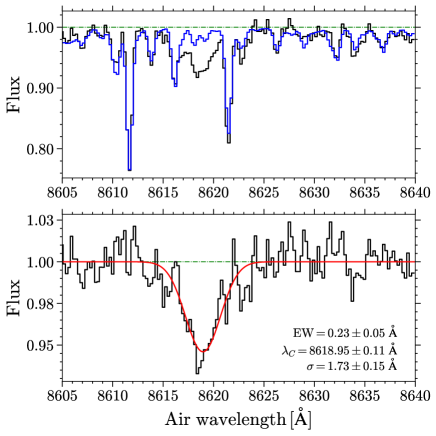
Figure 2: Fit of the DIB $\lambda$8620 in the spectrum of the GES target 06440722–0055038. Upper panel: Black and blue lines show the observed and synthetic spectra, respectively. Lower panel: Black line is the renormalized interstellar spectrum. The red line represents the fitted Gaussian profile. The measured EW, central wavelength ($\lambda_{C}$), and width ($\sigma$) are also indicated.

Table 1: Fit results of DIB $\lambda$8620 in the GIBS and GES data sets, as well as extinction, distance, and radial velocity of the background stars.

target ID	source	$\ell$	$b$	$\lambda_{C}\pm{\rm err}$	$\sigma\pm{\rm err}$	$\rm EW\pm{\rm err}$	$E(J\,{-}\,K_{\rm S})$	$d_{\rm star}$	$V_{\rm rad}$
		$(^{\circ})$	$(^{\circ})$	(Å)	(Å)	(Å)	(mag)	(kpc)	$(\rm km\,s^{-1})$
06432248–0046204	GES	–147.30	–2.15	$8622.46\,{\pm}\,0.02$	$0.80\,{\pm}\,0.03$	$0.063\,{\pm}\,0.026$	0.21	2.45	–5.62
06432400–0046576	GES	–147.29	–2.15	$8616.15\,{\pm}\,0.07$	$1.89\,{\pm}\,0.12$	$0.107\,{\pm}\,0.023$	0.19	3.24	171.91
06432685–0047112	GES	–147.28	–2.14	$8620.20\,{\pm}\,0.25$	$1.80\,{\pm}\,0.23$	$0.120\,{\pm}\,0.008$	0.22	3.09	54.54
06433215–0055203	GES	–147.15	–2.18	$8621.57\,{\pm}\,0.03$	$0.72\,{\pm}\,0.04$	$0.149\,{\pm}\,0.045$	0.26	0.55	11.40
06433789–0047286	GES	–147.25	–2.10	$8620.37\,{\pm}\,0.24$	$1.85\,{\pm}\,0.12$	$0.146\,{\pm}\,0.012$	0.25	5.22	64.12
06434241–0052100	GES	–147.18	–2.12	$8621.57\,{\pm}\,0.02$	$0.78\,{\pm}\,0.04$	$0.069\,{\pm}\,0.021$	0.13	1.11	12.63
06434513–0103076	GES	–147.01	–2.19	$8619.63\,{\pm}\,0.08$	$1.43\,{\pm}\,0.07$	$0.109\,{\pm}\,0.028$	0.25	4.33	69.55
06434800–0051432	GES	–147.17	–2.09	$8619.81\,{\pm}\,0.20$	$2.11\,{\pm}\,0.29$	$0.194\,{\pm}\,0.018$	0.35	5.58	65.63
06435592–0057034	GES	–147.08	–2.10	$8618.98\,{\pm}\,0.03$	$0.74\,{\pm}\,0.07$	$0.052\,{\pm}\,0.007$	0.21	2.08	97.97
06435624–0040198	GES	–147.32	–1.98	$8621.36\,{\pm}\,0.06$	$1.66\,{\pm}\,0.05$	$0.135\,{\pm}\,0.010$	0.18	1.50	36.71
$\cdots$
LRp8p4_F1_4094	GIBS	8.32	4.31	$8622.01\,{\pm}\,0.36$	$1.74\,{\pm}\,0.38$	$0.169\,{\pm}\,0.050$	0.46	7.56	–38.34
LRp8p4_F1_4343	GIBS	8.34	4.39	$8623.98\,{\pm}\,0.46$	$1.88\,{\pm}\,0.49$	$0.102\,{\pm}\,0.034$	0.48	7.24	–7.38
LRp8p4_F1_4355	GIBS	8.36	4.36	$8622.18\,{\pm}\,0.28$	$1.42\,{\pm}\,0.34$	$0.146\,{\pm}\,0.006$	0.52	7.29	–36.61
LRp8p4_F1_4379	GIBS	8.38	4.32	$8624.13\,{\pm}\,0.38$	$1.70\,{\pm}\,0.43$	$0.117\,{\pm}\,0.015$	0.40	7.80	–137.54
LRp8p4_F1_4393	GIBS	8.40	4.35	$8620.88\,{\pm}\,0.45$	$1.81\,{\pm}\,0.45$	$0.129\,{\pm}\,0.028$	0.44	7.81	–7.85
LRp8p4_F1_4399	GIBS	8.41	4.39	$8614.71\,{\pm}\,0.40$	$1.53\,{\pm}\,0.41$	$0.145\,{\pm}\,0.044$	0.49	7.76	182.51
LRp8p4_F1_4400	GIBS	8.41	4.35	$8622.18\,{\pm}\,0.29$	$1.59\,{\pm}\,0.40$	$0.243\,{\pm}\,0.022$	0.44	7.25	–22.18
LRp8p4_F1_4422	GIBS	8.33	4.28	$8614.35\,{\pm}\,0.41$	$1.52\,{\pm}\,0.42$	$0.109\,{\pm}\,0.017$	0.43	8.07	189.82
LRp8p4_F1_4424	GIBS	8.34	4.28	$8623.01\,{\pm}\,0.47$	$2.00\,{\pm}\,0.44$	$0.186\,{\pm}\,0.022$	0.41	7.75	13.02
LRp8p4_F1_4444	GIBS	8.37	4.25	$8618.93\,{\pm}\,0.39$	$1.68\,{\pm}\,0.56$	$0.118\,{\pm}\,0.018$	0.41	7.22	68.52
$\cdots$

Table 2: Selected GIBS and GES fields.

Field	($\ell_{0}$, $b_{0}$)	radius	source	DIB	$d_{\rm stellar}\pm{\rm err}$	$R_{\rm GC}^{\rm Reid19}\pm{\rm err}$	$R_{\rm GC}^{\rm Mroz19}\pm{\rm err}$	$d_{\rm los}\pm{\rm err}$
Nr	$(^{\circ})$	$(^{\circ})$		Nr	(kpc)	(kpc)	(kpc)	(kpc)
1	(8.5, 4.3)	0.2	GIBS	123	$7.68\,{\pm}\,0.41$	$4.69\,{\pm}\,0.45$	$4.87\,{\pm}\,0.36$	$3.57\,{\pm}\,0.48$
2	(5.0, 4.4)	0.2	GIBS	116	$7.30\,{\pm}\,0.37$	–	–	–
3	(–0.7, 4.5)	0.2	GIBS	116	$9.04\,{\pm}\,0.47$	$6.99\,{\pm}\,4.59$	$6.97\,{\pm}\,1.74$	–
4	(–3.4, 4.5)	0.1	GIBS	107	$8.58\,{\pm}\,0.44$	$5.06\,{\pm}\,1.30$	$5.33\,{\pm}\,1.12$	$3.17\,{\pm}\,1.19$
5	(–7.7, 4.5)	0.2	GIBS	101	$9.23\,{\pm}\,0.50$	$7.65\,{\pm}\,1.04$	$7.67\,{\pm}\,0.88$	–
6	(–0.3, –1.4)	0.2	GIBS	205	$7.44\,{\pm}\,0.91$	–	–	–
7	(8.5, –1.9)	0.1	GIBS	54	$7.45\,{\pm}\,0.55$	$6.48\,{\pm}\,0.47$	$6.44\,{\pm}\,0.39$	$1.80\,{\pm}\,0.48$
8	(2.4, –2.2)	0.1	GIBS	99	$7.80\,{\pm}\,0.46$	$4.18\,{\pm}\,0.98$	$4.67\,{\pm}\,0.86$	$3.86\,{\pm}\,0.99$
9	(0.3, –2.1)	0.1	GIBS	171	$7.58\,{\pm}\,0.81$	–	–	–
10	(–4.9, –2.0)	0.1	GIBS	128	$9.05\,{\pm}\,0.33$	$6.80\,{\pm}\,0.66$	$6.64\,{\pm}\,0.52$	$1.50\,{\pm}\,0.62$
11	(–7.5, –2.0)	0.2	GIBS	105	$9.16\,{\pm}\,0.46$	$7.17\,{\pm}\,0.57$	$7.01\,{\pm}\,0.45$	$0.93\,{\pm}\,0.52$
12	(–8.5, –6.1)	0.2	GIBS	63	$7.49\,{\pm}\,0.43$	$4.98\,{\pm}\,1.04$	$5.18\,{\pm}\,0.95$	$3.22\,{\pm}\,1.03$
13	(4.0, –6.0)	0.2	GIBS	48	$7.54\,{\pm}\,1.10$	–	–	–
14	(–4.0, –6.0)	0.2	GIBS	88	$9.24\,{\pm}\,0.65$	$7.86\,{\pm}\,3.13$	$7.63\,{\pm}\,1.36$	–
15	(–8.0, –6.0)	0.2	GIBS	55	$9.45\,{\pm}\,0.91$	$11.48\,{\pm}\,3.97$	$8.82\,{\pm}\,0.97$	–
16	(8.3, –8.5)	0.2	GIBS	54	$7.44\,{\pm}\,0.47$	$4.56\,{\pm}\,0.78$	$4.81\,{\pm}\,0.66$	$3.72\,{\pm}\,0.81$
17	(3.9, –8.6)	0.2	GIBS	55	$7.14\,{\pm}\,0.38$	–	–	–
18	(–0.4, –8.5)	0.2	GIBS	52	$7.47\,{\pm}\,0.35$	–	–	–
19	(–3.4, –8.6)	0.2	GIBS	20	$9.91\,{\pm}\,0.46$	$5.25\,{\pm}\,4.37$	$5.80\,{\pm}\,2.03$	–
20	(–7.7, –8.5)	0.2	GIBS	20	$9.29\,{\pm}\,0.62$	$4.60\,{\pm}\,2.55$	$5.34\,{\pm}\,1.73$	$3.49\,{\pm}\,1.78$
21	(–147.2, –2.0)	0.2	GES	22	$2.84\,{\pm}\,1.47$	$9.95\,{\pm}\,0.33$	$9.73\,{\pm}\,0.17$	$2.07\,{\pm}\,0.37$
22	(–33.4, 4.8)	0.2	GES	91	$8.80\,{\pm}\,1.67$	$6.80\,{\pm}\,0.20$	$6.66\,{\pm}\,0.06$	$1.76\,{\pm}\,0.27$
23	(–25.8, 5.0)	0.2	GES	48	$6.10\,{\pm}\,1.70$	$7.53\,{\pm}\,0.26$	$7.38\,{\pm}\,0.13$	$0.74\,{\pm}\,0.29$
24	(–27.7, 8.7)	0.2	GES	19	$5.84\,{\pm}\,2.09$	$8.35\,{\pm}\,0.43$	$8.20\,{\pm}\,0.36$	–
25	(–13.2, –5.5)	0.2	GES	28	$5.63\,{\pm}\,2.80$	$8.52\,{\pm}\,0.67$	$8.38\,{\pm}\,0.57$	–
26	(–9.8, –8.2)	0.4	GES	44	$5.21\,{\pm}\,1.98$	$9.67\,{\pm}\,1.47$	$9.08\,{\pm}\,0.68$	–
27	(–6.7, –6.2)	0.3	GES	24	$5.24\,{\pm}\,1.81$	$6.41\,{\pm}\,1.37$	$6.58\,{\pm}\,1.14$	$1.80\,{\pm}\,1.02$
28	(–3.7, –5.2)	0.2	GES	16	$4.77\,{\pm}\,2.11$	–	–	–
29	(1.0, –3.9)	0.3	GES	91	$4.86\,{\pm}\,2.13$	–	–	–
30	(0.2, –6.2)	0.2	GES	12	$6.78\,{\pm}\,2.05$	–	–	–
31	(–0.8, –9.5)	0.2	GES	13	$4.06\,{\pm}\,1.52$	–	–	–
32	(6.0, –9.7)	0.3	GES	40	$3.18\,{\pm}\,1.97$	$8.38\,{\pm}\,1.53$	$8.19\,{\pm}\,0.97$	–
33	(6.8, –8.8)	0.4	GES	24	$5.02\,{\pm}\,1.74$	$4.90\,{\pm}\,0.88$	$5.17\,{\pm}\,0.78$	$3.47\,{\pm}\,0.91$
34	(7.7, –6.0)	0.2	GES	27	$4.62\,{\pm}\,1.14$	$6.69\,{\pm}\,0.90$	$6.81\,{\pm}\,0.84$	$1.43\,{\pm}\,0.77$
35	(37.5, –8.7)	0.3	GES	41	$5.04\,{\pm}\,2.06$	$7.64\,{\pm}\,0.32$	$7.50\,{\pm}\,0.24$	$0.65\,{\pm}\,0.39$
36	(38.8, –6.8)	0.3	GES	25	$3.27\,{\pm}\,2.16$	$6.76\,{\pm}\,0.38$	$6.70\,{\pm}\,0.31$	$1.88\,{\pm}\,0.57$
37	(37.8, –6.7)	0.8	GES	112	$3.18\,{\pm}\,2.29$	$7.15\,{\pm}\,0.24$	$7.04\,{\pm}\,0.14$	$1.34\,{\pm}\,0.34$
38	(37.1, –7.7)	0.5	GES	83	$2.99\,{\pm}\,1.99$	$7.00\,{\pm}\,0.27$	$6.92\,{\pm}\,0.18$	$1.50\,{\pm}\,0.38$

3 Equivalent width and extinction

The tight linear correlation between EW and interstellar extinction for DIB $\lambda$8620 has been reported in many works (e.g., Wallerstein et al., 2007; Munari et al., 2008; Kos et al., 2013; Puspitarini et al., 2015) and also plays an important role in the study of the property of the DIB carrier. In Paper $\rm I$, we derived a linear relation of $E(J\,{-}\,K_{\rm S})\,{=}\,1.884\,({\pm}\,0.225)\,{\times}\,{\rm EW}\,{-}\,0.012\,({\pm}\,0.072)$ with a pure RC sample, where EW was the median value in each GIBS field and $E(J\,{-}\,K_{\rm S})$ in each field was derived based on the peak color estimated by the VVV–DR2 catalog (Minniti et al., 2017) and intrinsic color given by Gonzalez et al. (2011). In this section, we briefly describe our measurements of the EW and the $E(J\,{-}\,K_{\rm S})$ for the GES targets, while we use the results from Paper $\rm I$ for GIBS targets.

3.1 EW measurement

As the DIB profile is fitted by a Gaussian function in our procedures, the EW can be calculated by the fitted depth ($D$) and width ($\sigma$), $\rm EW\,{=}\,\sqrt{2\pi}\,{\it D}\,\sigma$. The error of EW is estimated using the same method as described in Paper $\rm I$, considering the contribution of both the random noise (i.e., S/N) and the error based on the discrepancy between the observed and the synthetic spectrum. Puspitarini et al. (2015) also analyzed the DIB $\lambda$8620 in 162 GES spectra. Due to the low S/N of these spectra, only 43 passed our quality-flag criteria $(\rm QF\,{>}\,0)$. Figure 3 shows the comparison of the EW for these 43 stars where Puspitarini et al. (2015) systematically obtained slightly larger EW than the result in this work, with a mean difference of 0.031 Å and a standard deviation of 0.022 Å. The mean difference is similar to the average error of EW in this work (0.020 Å) and in that of Puspitarini et al. (2015, 0.045 Å). The systematic difference might be caused by the use of different synthetic spectra in Puspitarini et al. (2015) and this work. Specifically, the synthetic model used in Puspitarini et al. (2015) was based on an the ATLAS 9 model atmosphere and the SYNTHE suite (Kurucz, 2005; Sbordone et al., 2004; Sbordone, 2005), which is different from the MARCS model atmospheres (Gustafsson et al., 2008) used in this work. The different fit methods also contribute to the discrepancy in EW, that is we applied a Gaussian fit to the DIB profile, while Puspitarini et al. (2015) fitted the DIB feature with an empirical model averaging the profiles detected in several spectra based on the data analysis reported by Chen et al. (2013).

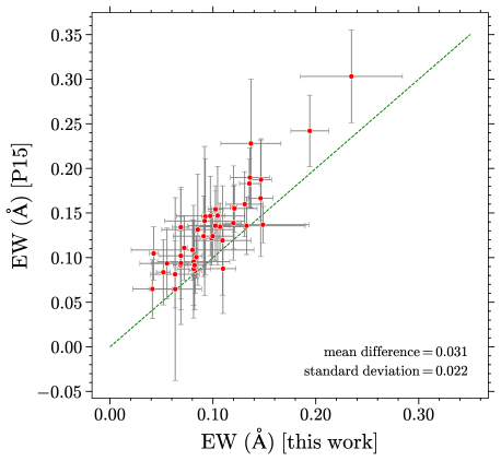
Figure 3: Comparison of the EW computed in this work with the one from Puspitarini et al. (2015) for 43 common targets. The dashed green line traces the one-to-one correspondence.

3.2 Extinction

The distances to and the individual reddenings of the GES stars were calculated by the spectro-photometric method described in Rojas-Arriagada et al. (2017, hereafter R17), using the stellar parameters ($T_{\rm eff}$, ${\rm log}\,g$, $\rm[Fe/H]$) with the corresponding errors together with the PARSEC isochrones (Marigo et al., 2017). The extinction of our GIBS sample was derived by the high-resolution extinction map from Surot et al. (2020, hereafter S20) using RGB+RC stars from the VVV survey (Minniti et al., 2010). We refer the reader to Paper $\rm I$ for a more detailed description. Figure 4 shows the comparison between $E(J\,{-}\,K_{\rm S})$ calculated by R17 and S20 for 1626 GES sample stars with $|\ell|\,{\leqslant}\,10^{\circ}$. The derived $E(J\,{-}\,K_{\rm S})_{\rm R17}$ is systematically larger than that of $E(J\,{-}\,K_{\rm S})_{\rm S20}$ with a mean difference $\rm(R17-S20)$ of 0.056 mag and a standard deviation of 0.082 mag. As this difference between R17 and S20 is smaller than the variation of $E(J\,{-}\,K_{\rm S})$ in each field, we did not attempt to correct for this.

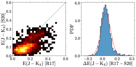
Figure 4: Left panel: Comparison between $E(J\,{-}\,K_{\rm S})$ derived by R17 and S20. The dashed green line traces the one-to-one correspondence. The color represents the number density. Right panel: Distribution of the differences between R17 and S20. The red line represents a Gaussian fit.

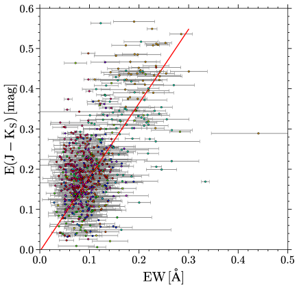
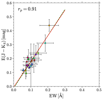
Figure 5: Correlation between EW and $E(J\,{-}\,K_{\rm S})$ derived from GES individual targets (left) and fields (right). The dots with the same color are from the same field, and their median value shown in right panel is colored in the same way. The dashed green line in the right panel shows the relation derived by Paper $\rm I$. The error bars indicate the standard deviation in each field. The red lines in both panels are fit to the dots in the right panel. The Pearson correlation coefficient ($r_{p}$) is also indicated.

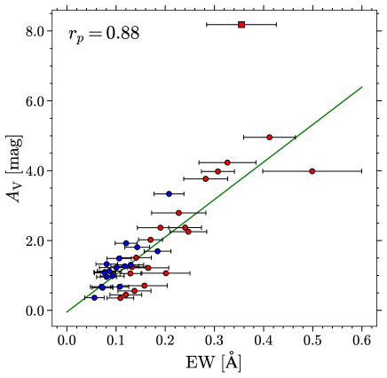
Figure 6: Correlation between EW and $A_{\rm V}$ (SFD) for the median values in each GIBS (red) and GES (blue) field. The green line represents the linear fit, excluding the field with $A_{\rm V}\,{>}\,8$ mag (the red square). The Pearson correlation coefficient ($r_{p}$) is also indicated.

3.3 Correlation between EW and extinction

Figure 5 shows the correlation between EW and $E(J\,{-}\,K_{\rm S})$ for the individual GES targets (left panel) and the median values for each field (right panel). Although a large dispersion is found for individual measurements, the median EW and $E(J\,{-}\,K_{\rm S})$ for each field present a tight correlation with a Pearson correlation coefficient ($r_{p}$) of 0.91. The linear relation is derived as $E(J\,{-}\,K_{\rm S})\,{=}\,1.842\,({\pm}\,0.203)\,{\times}\,{\rm EW}\,{-}\,0.005\,({\pm}\,0.023)$, which is highly consistent with the relation recommended by Paper $\rm I$ for the GIBS fields (the dashed green line in Fig. 5), even when taking into account the different resolutions between the GES ($R\,{\sim}\,16,200$) and GIBS ($R\,{=}\,6500$) spectra and the difference between $E(J\,{-}\,K_{\rm S})_{\rm R17}$ and $E(J\,{-}\,K_{\rm S})_{\rm S20}$. For the latter, the reasons are 1) the recommended relation in Paper $\rm I$ was derived using an RC-based $E(J\,{-}\,K_{\rm S})$ (which is not from the S20 map), although $E(J\,{-}\,K_{\rm S})_{\rm S20}$ was used for GIBS individual targets. We emphasize here again that in Paper $\rm I$ we derived the relation in three ways, two of them were based on the median $E(J\,{-}\,K_{\rm S})_{\rm S20}$ in each field, but the preferred one used the RC-based $E(J\,{-}\,K_{\rm S})$; and 2) we applied a cut of $E(J\,{-}\,K_{\rm S})\,{>}\,0.25$ mag as described in Paper $\rm I$, and the typical $E(J\,{-}\,K_{\rm S})_{\rm R17}$ of GES fields are within 0.3 mag as they are located at higher Galactic latitudes (see Fig. 1). Thus, the two relations were derived in different $E(J\,{-}\,K_{\rm S})$ ranges. Their consistency might indicate a decrease of the difference between R17 and S20 for higher $E(J\,{-}\,K_{\rm S})$. For the further analysis, we use as in Paper $\rm I$ the median quantities for each GES field rather than the individual measurements.

Additionally, we also find a linear relation ($r_{p}$=0.88) between EW and $A_{\rm V}$ derived from the SFD map with a calibration by Schlafly & Finkbeiner (2011), except for the GIBS field #7 located at $(\ell,\,b)\,{=}\,(8.5^{\circ},\,{-}1.9^{\circ}),$ where the corresponding $A_{\rm V}$ is clearly overestimated. This outlier is due to the fact that at low galactic latitudes, the SFD map may not be reliable. Indeed, a comparison with S20 reveals much lower extinction values for this field ($A_{\rm V}\,{\sim}\,4\,$mag). The linear fit yields a coefficient of $A_{\rm V}/{\rm EW}\,{=}\,10.733\,{\pm}\,0.972$. With the relation in NIR band $E(J\,{-}\,K_{\rm S})/{\rm EW}\,{=}\,1.884$, we obtain $E(J\,{-}\,K_{\rm S})/A_{\rm V}\,{=}\,0.176$, slightly higher than the ratio of 0.170 predicted by the CCM model (Cardelli et al., 1989) with $R_{\rm V}\,{=}\,3.1$. On the other hand, the tight correlation with extinction makes DIB $\lambda$8620 a powerful tracer of any possible extinction law variation for different lines of sight. However, Krełowski (2018) argued the variation of the ${\rm EW}/E(B\,{-}\,V)$ ratio for DIB $\lambda$8620 by two stars HD 204827 and HD 219287 which have similar $E(B\,{-}\,V)$ but very different DIB profiles (see Fig. 11 in his paper).

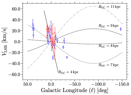
Figure 7: Longitude–velocity ($\ell-V_{\rm LSR}$) diagram for the GIBS (red) and GES (blue) fields, respectively. The circles indicate the median $V_{\rm LSR}$ and standard error of the mean for each field. Velocity curves calculated by Model A5 in Reid et al. (2019) for different galactocentric distances ($R_{\rm GC}$) are overplotted.

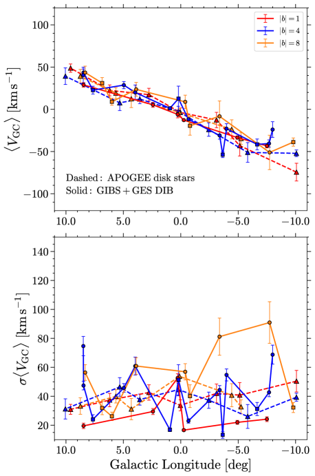
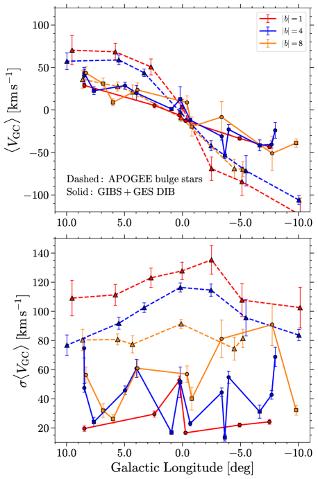
Figure 8: Median galactocentric radial velocity (top) and velocity dispersion (bottom) calculated in GIBS fields (circles), GES fields (squares), and APOGEE bins (triangles), as a function of Galactic longitude, for different latitudes marked with different colors. The APOGEE stars used in the left panels are in the disk with line-of-sight distances smaller than 3 kpc. Bulge stars ($R_{\rm GC}\,{\leqslant}\,3$ kpc) are used in right panels.

4 Kinematics of the DIB carrier

4.1 Rest-frame wavelength

As the most important observational parameter, the precise DIB rest-frame wavelength ($\lambda_{0}$) is required for inferring the kinematic information of the DIB carrier. Although without a physical identification of the carrier, $\lambda_{0}$ can be determined with the empirical assumption that the radial velocity toward the Galactic center or the Galactic anti-center (see Zasowski et al. 2015) is essentially null. Similarly to Paper $\rm I$, 603 DIBs with $-3^{\circ}\,{<}\,b\,{<}\,3^{\circ}$ and $-6^{\circ}\,{<}\,\ell\,{<}\,3^{\circ}$ are selected from our pure GIBS sample which includes only the most reliable measurements (i.e., the error in EW is small). We obtained a median central wavelength in the heliocentric frame of $8620.52\,{\pm}\,0.36$ Å, close to the results of Paper $\rm I$ and Munari et al. (2008).

However, both of the previous works did not consider the effect of the solar motion toward the Galactic center. Therefore, the rest-frame wavelength in the Local Standard of Rest (LSR) should be derived as $\lambda_{0}\,{=}\,\frac{c}{c-U_{\odot}}\cdot C_{\rm obs,}$ where $c$ is the speed of light, $C_{\rm obs}$ the measured central wavelength in the heliocentric frame, and $U_{\odot}$ the solar motion toward the Galactic center. In this work, we assume $U_{\odot}\,{=}\,10.6\,{\pm}\,1.2\,\rm km\,s^{-1}$ (Reid et al., 2019, Model A5) which gives a $\lambda_{0}\,{=}\,8620.83$ Å that is in good agreement with the value of 8620.79 Å in Galazutdinov et al. (2000). However, the solar motion $U_{\odot}$ can vary between $10.1\,{\pm}\,1.0\,\rm km\,s^{-1}$ (Mróz et al., 2019), $10.3\,\rm km\,s^{-1}$ (Bovy et al., 2012), $10.6\,{\pm}\,1.2\,\rm km\,s^{-1}$ (Reid et al., 2019), $10.7\,{\pm}\,1.8\,\rm km\,s^{-1}$ (Reid et al., 2014), and $11.1\,\rm km\,s^{-1}$ (Reid & Brunthaler, 2004; Schönrich et al., 2010). For an exhaustive summary of the measurements of the solar motion, we refer the reader to Wang et al. (2021). We note that a difference of $\Delta U_{\odot}\,{=}\,1\,\rm km\,s^{-1}$ causes an error of $\sim$0.03 Å in $\lambda_{0},$ while the typical error of $C_{\rm obs}$ in the fit is about 0.36 Å.

4.2 Distribution of the carrier velocities

We investigate here the radial velocity of the DIB carrier with respect to the LSR, $V_{\rm LSR}=V_{\rm HC}+\@vec{V_{\sun}}\,{\cdot}\,\@vec{A}$, where $\@vec{V_{\sun}}=(10.6,10.7,7.6)\,\rm km\,s^{-1}$ is the solar motion fitted by Model A5 of Reid et al. (2019), and $\@vec{A}\,{=}\,(\cos(b)\cos(\ell),\cos(b)\sin(\ell),\sin(b))$ is the directional array of the DIB carrier. Figure 7 presents $V_{\rm LSR}$ as a function of Galactic longitude for the GIBS (red circles) and GES (blue circles) fields, respectively, where we show the median $V_{\rm LSR}$ in each field. The error bars show the standard error of the mean (${\rm SEM}\,{=}\,\sigma/\sqrt{N}$, $N$ is the sample size) in each field. Indicated are Galactic rotation curves computed by Model A5 in Reid et al. (2019) with different galactocentric radii ($R_{\rm GC}$).

Limited by the available sightlines, we cannot find a clear Galactic rotation from the GIBS$/$GES fields as seen in Zasowski et al. (2015, Figure 8). Moreover, fields with $|\ell|\,{\leqslant}\,10^{\circ}$ present a large velocity dispersion caused by both the fitting errors (an error of 0.36 Å in $C_{\rm obs}$ amounts to $\Delta V_{\rm LSR}\,{\sim}\,10\,\rm km\,s^{-1}$) and the velocity crowding (Wenger et al., 2018). In Sect. 5, we apply two Galactic rotation models in order to derive kinematic distance for the DIB carrier.

4.3 Galactocentric velocity and velocity dispersion

One of the known kinematic characteristics of the Galactic boxy/peanut bulge is its cylindrical rotation, which has already been investigated in many studies (see e.g., Ness et al., 2013; Zoccali et al., 2014; Rojas-Arriagada et al., 2020). This rotation curve is steeper in the bulge than for the Galactic disk (see e.g., Howard et al., 2009; Shen et al., 2010; Zoccali et al., 2014). In contrast, the velocity dispersion in the bulge is higher with respect to the Galactic disk (by a factor of two or more), indicating more isotropic kinematics. Using these kinematic properties, we can determine if the DIB carriers are associated with the background stars or in the foreground disk. Here, we investigate the validity of this assumption. We use the APOGEE DR16 data set (Majewski et al., 2017) as a comparison sample, and in particular the Galactic bulge sample from Rojas-Arriagada et al. (2020) with $|\ell|\,{\leqslant}\,11^{\circ}$, for three different Galactic latitude bins $|b|\,{=}\,1^{\circ},\,4^{\circ},\,8^{\circ}$. As shown by Rojas-Arriagada et al. (2020), a simple cut at $R_{\rm GC}\,{\leqslant}\,3.5$ kpc ensures a reliable bulge sample, which we applied.

Furthermore, we define a typical “Galactic disk” sample of APOGEE within the same longitude and latitude range as the bulge sample but with line-of-sight distances within 3 kpc. The distances of our APOGEE stars were calculated by the same method used in Rojas-Arriagada et al. (2020) using the spectro-photometric distances together with PARSEC isochrones (Rojas-Arriagada et al., 2017). $V_{\rm HC}$ has been transformed to Galactocentric velocities ($V_{\rm GC}$) using the following formula (e.g., Ness et al., 2013; Zoccali et al., 2014), where $(\ell,b)$ are the galactic coordinates:

$$\begin{split}V_{\rm GC}=V_{\rm HC}&+220\,{\rm sin}(\ell)\,{\rm cos}(b)\\ &+16.5[{\rm sin}(b)\,{\rm sin(25)}+{\rm cos}(b)\,{\rm cos}(25)\,{\rm cos}(\ell-53)]\end{split}.$$ (1)

Figure 8 shows the rotation curves and velocity dispersion for the APOGEE sample (dashed lines) as well as our DIB measurements (solid lines). The APOGEE stars at different latitudes are further separated into eight equal longitude bins, where the median $V_{\rm GC}$ in each bin is used. Our full sample (GES and GIBS) has been divided into three groups with $|b|\,{<}\,3^{\circ}$, $3^{\circ}\,{<}\,|b|\,{<}\,7^{\circ}$ and $7^{\circ}\,{<}\,|b|\,{<}\,10^{\circ}$. The right panel of Fig. 8 shows the comparison between the bulge sample of APOGEE stars and our DIB samples. It is evident that in terms of rotation and velocity dispersion, our DIB measurements do not follow the general bulge characteristics of the stars. This is most striking in the velocity dispersion where the DIBs show more than a factor of two smaller velocity dispersion with respect to the bulge stars. In the left panel of Fig. 8, we see, on the other hand, a much better agreement, with the disk sample from APOGEE showing similar velocity dispersion and rotation velocities. We therefore conclude that the DIB carriers located inside the Galactic disk ($4\,{<}\,R_{\rm GC}\,{<}\,11$ kpc) could be far away from the background stars and much closer to us.

5 Distance of the DIB carrier

As an interstellar feature, the DIB profile measured in the spectrum of a background star is the result of an integration of the DIB carrier between the observer and the star. The distance of the background star is then an upper limit on the typical distance of the DIB carrier along the sight line (Zasowski et al., 2015). Based on hundreds of thousands spectra, Kos et al. (2014) and Zasowski et al. (2015) built 3D intensity maps for DIB $\lambda$8620 and DIB $\lambda$15273, respectively, using stellar distances and tracing the cumulation and variation of the DIB carriers along substantial sight lines. Their pioneering works encourage the following studies with large spectroscopic surveys, while in this work we attempt to estimate the distance of the DIB carrier more “directly” by the carrier radial velocity and Galactic rotation model; that is, the kinematic distance.

5.1 Kinematic distance

We calculated the kinematic distance of the DIB carrier using the median $V_{\rm LSR}$ in each field together with two different Galactic rotation models. One is a two-parameter “universal” rotation model (Model A5 in Reid et al., 2019), the other is a linear rotation model (Model 2 in Mróz et al., 2019). For Model A5 in Reid et al. (2019), the kinematic distance is computed with a Monte Carlo method introduced by Wenger et al. (2018), using their python package kd and considering the error of $V_{\rm LSR}$ as well as the parameter uncertainty of the rotation model. For Model 2 in Mróz et al. (2019), only the error of $V_{\rm LSR}$ is considered. Figure 9 shows the comparison between the estimated galactocentric distances $R_{\rm GC}$ derived by the two models for our sample, which give consistent results with slightly larger distances for Mróz et al. (2019) within $4\,{<}\,R_{\rm GC}\,{<}\,6$ kpc, while these are smaller for $R_{\rm GC}\,{>}\,9$ kpc. As both Reid et al. (2019) and Mróz et al. (2019) fit the models mainly within the 4–15 kpc range, kinematic distances in the inner Galaxy with $R_{\rm GC}\,{<}\,4$ kpc are not reliable and should not be used. In addition, in the inner Galaxy the orbits of the stars are highly eccentric (see e.g., Rojas-Arriagada et al. 2020), causing large errors for the kinematic distances.

We also calculated the line-of-sight distance:

$$d_{\rm los}=R_{\odot}\cdot{\rm cos}(\ell)\pm\sqrt{R_{\rm GC}^{2}-R_{\odot}^{2}\cdot{\rm sin^{2}}(\ell)},$$ (2)

where $R_{\odot}=8.15$ kpc (Reid et al., 2019), $\ell$ is the median Galactic latitude of each field, and for $R_{\rm GC}$ we use the results from the model of Reid et al. (2019). The calculation was also completed by the kd package. For the inner Galaxy, Eq. 2 gives two possible solutions, of which we always chose the closest one. In case where the solution is negative or has no rational solution, the result has been dropped.

Finally, we obtained $R_{\rm GC}\,{>}\,4$ kpc for 14 GIBS and 14 GES fields. Nine GIBS and ten GES fields had valid $d_{\rm los}$. These measurements, together with their uncertainties, are listed in Table 2. A face-on view of the distribution of the fields with valid $d_{\rm los}$ is shown in Fig. 10. The fields within $|\ell|\,{<}\,10^{\circ}$ experience large uncertainties than the fields outside. Seven fields are located within or beyond the Scutum–Centaurus Arm, while 11 other fields are around the Sagittarius Arm and the Orion Spur. The only field toward the Galactic anti-center at $(\ell,\,b)=({-}147.2^{\circ},\,{-}2.0^{\circ})$ almost reaches the edge of the Perseus Arm.

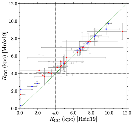
Figure 9: Comparison between kinematic distances derived by Model 2 in Mróz et al. (2019) and Model A5 in Reid et al. (2019). The red and blue dots indicate the GIBS and GES fields, respectively. The dashed green line traces the one-to-one correspondence. The dashed black lines indicate $R_{\rm GC}=4$ kpc.

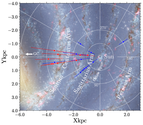
Figure 10: Face-on view of the spatial distribution of nine GIBS and ten GES fields with valid $d_{\rm los}$; i.e., the kinematic distance of the DIB carrier calculated by the field-median radial velocity and model A5 in Reid et al. (2019), overplotted with the Milky Way sketch created by Robert Hurt and Robert Benjamin (Churchwell et al., 2009). The Galactic center is located at $(-8,0)$. Red and blue dots indicate the GIBS and GES fields, respectively.

5.2 Comparison with stellar distances

The distances to the background stars are the upper limit on the carrier distances and can be used to test the reliability of our distance measurements. As the targets in the GIBS sample are RC stars, we can calculate their distance assuming $M_{\rm K_{S}}\,{=}\,-1.61$ mag (Ruiz-Dern et al., 2018) and $(J-K_{\rm S})_{0}\,{=}\,0.674$ mag (Gonzalez et al., 2012). For the GES sample, we used spectro-photometric distances (see Sect. 2). For each field, we calculated the median distance together with its standard deviation. The results are shown in Table 2 for field medians and Table 1 for individual stars (some examples; full catalog can be accessed online). For a test, we also cross-matched the GES sample with the catalog of Gaia–EDR3 (Gaia Collaboration et al., 2021) within 1″and used the photogeometric distances estimated by Bailer-Jones et al. (2021) from the Gaia parallaxes. The resulting median distances for each field are consistent with our calculations within the distance uncertainties.

Figure 11 displays the comparison between the median stellar distances and the kinematic distance of the DIB carrier for nine GIBS and ten GES fields with valid $d_{\rm los}$. All of the points lie below the identity line (dashed green), indicating all the estimated carrier distances are smaller than the stellar distances. This is not very surprising for GIBS as the RC stars in GIBS fields are mainly distributed in the Galactic bulge, and we required the nearer solution for $d_{\rm los}$. It is more interesting for GES fields, of which the median distances are much closer to the Sun, meaning that the kinematic distance of the DIB carrier is still smaller than the stellar distance. This confirms the reliability of the derived kinematic distance to some extent. While we still need to emphasize that kinematic distances are of high uncertainty in the direction of the Galactic center and the Galactic anti-center (see e.g., Balser et al., 2015; Wenger et al., 2018) and need to be carefully used.

The comparison in Fig. 11 also demonstrates that the DIB carrier can be located much closer to the observer than the background stars. So, when we make use of DIBs as a tool to trace the ISM environments and Galactic structure, such as local ISM medium (Piecka & Paunzen, 2020), Galactic arms (Puspitarini & Lallement, 2019), and Galactic warp (Istiqomah et al., 2020), target stars at distant zones and/or high latitudes require more attention.

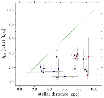
Figure 11: Comparison between stellar distance and the kinematic distance of the DIB carrier for nine GIBS (red dots) and ten GES fields (blue dots). The dashed green line traces the one-to-one correspondence.

6 Comparison with the NIR DIB$\,\lambda$15273

The correlation between different DIBs is one of the most important methods to study the relations of their carriers and to find the common carrier for a set of DIBs (see Elyajouri et al. 2017, 2018, Sonnentrucker et al. 2018, Galazutdinov et al. 2020, and Bondar 2020 for some recent studies). The tightest correlation is between DIB $\lambda$6196 and DIB $\lambda$6614 (McCall et al., 2010), although the conclusion of their common origin still encounters some problems (Krełowski et al., 2016). Elyajouri et al. (2017) reported tight correlations between the strong NIR DIB at $1.5273\,\rm\mu m$ and the weak DIBs in its vicinity ($\lambda$15617, $\lambda$15653, and $\lambda$15673), as well as some strong optical DIBs, proposing DIB $\lambda$15273 as a good tracer of the interstellar environments.

In this section, we make a simple comparison between DIB $\lambda$8620 measured in this work and DIB $\lambda$15273 in the APOGEE spectra measured by Zasowski et al. (2015). We accessed the full APOGEE DIB catalog with 49,474 entries, but cross-matched them with our GIBS$/$GES sample within 1″, where only 16 common targets were found (GES). This is due to the fact that APOGEE and GIBS$/$GES trace different stellar populations in their target selection; that is GIBS trace RC stars, while APOGEE traces brighter and cooler giants on the RGB. Therefore, we selected the APOGEE DIBs based on the same fields with respect to GIBS and GES and compared their median EW in each field. In total, we find six GES and three GIBS fields matching the APOGEE footprint. Figure 12 shows the comparison between the EW of the two DIBs where a linear relation between the two carriers can be found ($r_{p}\,{=}\,0.90$). Clearly, more observations of these two DIB carriers spanning a larger EW range are needed in order to draw firmer conclusions. A linear fit to all the fields yields a ratio of $\rm EW\,\lambda 15273/EW\,\lambda 8620\,{=}\,1.411\,{\pm}\,0.242$, demonstrating that the DIB $\lambda$15273 is stronger than DIB $\lambda$8620.

It should be noted that Elyajouri & Lallement (2019) reported measurements of DIB $\lambda$15273 that were systematically weaker than those in Zasowski et al. (2015) due to the use of different stellar models. With their results, DIB $\lambda$8620 would be oppositely larger than the DIB $\lambda$15273, with a ratio of $\rm EW\,\lambda 15273/EW\,\lambda 8620\,{=}\,0.670\,{\pm}\,0.132$ ($r_{p}\,{=}\,0.75$, see triangles in Fig. 12; the fields are selected with the same method for Zasowski et al. 2015). However, this correlation was built only with the median values in very few common fields. Thus, the present result is still a rough one, and further investigations with bigger data sets are expected. The correlation between DIB $\lambda$8620 and DIB $\lambda$15273, as well as other optical and infrared DIBs, will benefit from forthcoming new large spectroscopic data. The DIB $\lambda$8620 shows a promising diagnostic of the interstellar conditions and a tracer of the Galactic structure.

We derived a linear correlation between EW and $A_{\rm V}$ with ${\rm EW}\,\lambda 8620/A_{\rm V}\,{=}\,0.093$ Å $\rm mag^{-1}$ for our GIBS$/$GES fields (Sect. 3.3). Compared to ${\rm EW}\,\lambda 15273/A_{\rm V}\,{=}\,0.102$ Å $\rm mag^{-1}$ from Zasowski et al. (2015), we can obtain a ratio of 1.097 for $\rm EW\,\lambda 15273/EW\,\lambda 8620$, which is about 22% lower than the value from the direct EW comparison with Zasowski et al. (2015). This difference could be caused by the different extinction sources used in Zasowski et al. (2015) and this work; Zasowski et al. (2015) applied the RJCE method (Majewski et al., 2011) for their extinction values, while we used the $A_{\rm V}$ from the SFD map with a calibration of Schlafly & Finkbeiner (2011).

Zasowski et al. (2015) roughly estimated the carrier abundance relative to hydrogen for DIB $\lambda$15273 as $N_{\rm DIB}/N_{\rm H}\sim 2.3\times 10^{-11}/f$ with its relationship to $A_{\rm V}$, $\lambda_{0}=15272.42$ Å, and a mean hydrogen-to-extinction relation of $N_{\rm H}/A_{\rm V}=2\times 10^{21}\,{\rm cm^{-2}\,mag^{-1}}$ (Dickey & Lockman, 1990), where $f$ is the transition oscillator strength (e.g., Spitzer, 1978). With our derived relation ${\rm EW}\,\lambda 8620/A_{\rm V}=0.093$ Å $\rm mag^{-1}$ and $\lambda_{0}=8620.83$ Å, the carrier abundance for DIB $\lambda$8620 is estimated as $1.4\times 10^{-11}/f$, slightly lower than the value of the DIB $\lambda$15273.

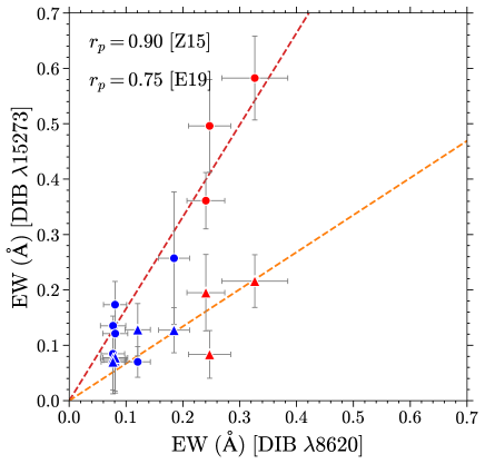
Figure 12: Median EW comparison between DIB $\lambda$8620 and DIB $\lambda$15273 for GIBS (red) and GES (blue) fields. Filled circles indicate the DIB $\lambda$15273 measured by Zasowski et al. (2015) and triangles by Elyajouri & Lallement (2019). The dashed red line is the fit between the GIBS$/$GES sample and the Zasowski et al. (2015) sample, and the dashed orange line between GIBS$/$GES and Elyajouri & Lallement (2019). The error bars represent the standard deviation in each field. The Pearson correlation coefficients ($r_{p}$) are also indicated.

7 Conclusions and summary

In this work, we successfully detected the DIB $\lambda$8620 in 760 GES spectra with $|b|\,{\leqslant}\,10^{\circ}$ and $\rm S/N\,{>}\,50$. Their EW, as well as depth, central wavelength, and width, were measured with a Gaussian profile. Our EWs were slightly smaller than those measured in Puspitarini et al. (2015), with a mean difference of 0.031 Å for 43 common targets. The linear relation between EW and $E(J\,{-}\,K_{\rm S})$ ($r_{p}=0.91$) derived from field median values is highly consistent with the recommended correlation derived in Paper $\rm I$.

Combined with a pure GIBS sample from Paper $\rm I$, we confirmed a linear relation between EW and $A_{\rm V}$ (SFD) with $r_{p}=0.88$, using 2540 DIBs distributed in 38 fields. We obtained $E(J\,{-}\,K_{\rm S})/A_{\rm V}\,{=}\,0.176$ from their linear fit with EW, which was slightly higher than the ratio of 0.170 predicted by the CCM model (Cardelli et al., 1989). Furthermore, the rest-frame wavelength of DIB $\lambda$8620 was redetermined as $\lambda_{0}=8620.83\pm 0.36$ Å after the consideration of the solar motion.

We also studied the kinematics of the DIB carriers based on the median radial velocities in each field. Most of our fields distributed close to the Galactic center ($|\ell|\,{\leqslant}\,10^{\circ}$), thus they were crowded in the $\ell-V_{\rm LSR}$ diagram with large scatters. The $\ell-V_{\rm GC}$ diagram showed that the DIB carriers mainly occupied in the local Galactic disk as traced by a sample of APOGEE stars.

Applying the Galactic rotation models (Reid et al., 2019; Mróz et al., 2019), we calculated the kinematic distances of the DIB carriers for each field and got valid line-of-sight distances ($d_{\rm los}$) for nine GIBS and ten GES fields. All derived $d_{\rm los}$ are smaller than the median distances to background stars in each field. It demonstrates that the DIB carriers can be located much closer to us than the background stars. Therefore, when we make use of target stars to build the integrated DIB map, we have to be careful with the distant- and/or high-latitude zones, as well as the region where stars are not well sampled.

For the first time, we roughly investigated the mutual correlation between DIB $\lambda$8620 measured in this work and DIB $\lambda$15273 in Zasowski et al. (2015) and Elyajouri & Lallement (2019), respectively, with three GIBS fields and six GES fields, resulting in a liner coefficient of $\rm EW\,\lambda 15273/EW\,\lambda 8620\,{=}\,1.411\,{\pm}\,0.242$ for the measurements from Zasowski et al. (2015) and $0.670\,{\pm}\,0.132$ for Elyajouri & Lallement (2019). The Pearson correlation coefficients are 0.90 and 0.75, respectively. The difference was caused by the use of different stellar templates for APOGEE spectra. The linear correlation suggested that DIB $\lambda$8620 may also correlate with other optical and infrared DIBs such as DIB $\lambda$15273, which can be used to trace the interstellar environments and Galactic structure with the measurements in large spectroscopic surveys.