Positron energy distribution in factorized trident process

Abstract

We estimate the energy distribution of positrons produced in the interaction of ultra-relativistic electrons with a high-intensity laser beam. The underlying trident process is factorized on the probabilistic level. That is, we deploy a two-step mechanism for the formation of electron-positron pairs. In the first step, a high-energy photon is produced as a result of nonlinear Compton scattering. In the second step, an electron-positron pair is created by the nonlinear (multi-photon) Breit-Wheeler process.

I Introduction

Our study is devoted to an analysis of the energy spectra of positrons ($e^{+}$) produced in collisions of ultra-relativistic electrons ($e^{-}$) with a high-intensity laser beam (${\cal L}$, circular polarization), $e^{-}+{\cal L}\to{e^{-}}^{\prime}+e^{+}e^{-}$, where ${e^{-}}^{\prime}$ is the recoil electron. This is the trident process which, analog to the nonlinear two-photon Compton process Loetstedt:2009zz ; Seipt:2012tn ; Mackenroth:2012rb , is described within the Furry picture by a prototypical two-vertex diagram and its exchange part. Quantum interference effects make a throughout description quite challenging. Correspondingly, a series of papers, e.g. Ilderton:2010wr ; Hu:2010ye ; King:2013osa ; King:2013zw ; Dinu:2017uoj ; Torgrimsson:2020wlz ; Dinu:2019wdw ; Dinu:2019pau ; Torgrimsson:2020gws ; King:2018ibi ; Mackenroth:2018smh , analyzed in depth the many interesting facets of trident VIRitus ; VNBaier as a fundamental strong-field QED process. Trident is to be considered as the fist stage of the development of QED cascades and plays thus a prominent role, also for testing numerical simulation codes Gonoskov:2014mda ; DiPiazza:2018bfu ; Gonoskov:2021hwf , in particular in the strong-field regime. The increasing interest is documented by a number of plans of experimental facilities E_320 ; Meuren:2020nbw ; Abramowicz:2019gvx ; Abramowicz:2021zja ; Salgado:2021fgt enabling high-precision measurements after the pioneering work of E-144 Bamber:1999zt ; Burke:1997ew and successors Cole:2017zca ; Poder:2018ifi .

In view of these developments, an easily usable approximation of trident should be devised. Following suggestions in Torgrimsson:2020wlz ; Dinu:2019pau ; Dinu:2019wdw and in line with earlier approaches King:2013osa ; King:2013zw ; Hu:2010ye ; Bamber:1999zt , we apply a folding model of type n$\ell$C $\otimes$ n$\ell$BW, i.e. gluing the probabilities of nonlinear Compton (n$\ell$C) and nonlinear Breit-Wheeler (n$\ell$BW) processes as depicted by the Furry picture diagrams
                                         (double lines: Volkov wave functions, vertical lines: photon propagator or real unpolarized photon with frequency $\omega^{\prime}$). This is the incoherent product of two one-vertex processes in the spirit of kinetic simulations, cf.  Elkina:2010up ; Seipt:2020uxv , which is realized here by the convolution

$$\int d\omega^{\prime}\frac{d\Gamma_{n\ell C}^{e^{-}+{\cal L}\to\gamma^{\prime}(\omega^{\prime})+{e^{-}}^{\prime}}}{d\omega^{\prime}}\,\Gamma_{n\ell BW}^{\gamma^{\prime}(\omega^{\prime})+{\cal L}\to e^{+}e^{-}}$$ (1)

of n$\ell$C and n$\ell$BW probabilities or rates $\Gamma_{n\ell C,n\ell BW}$ (see also equation (21) in King:2013osa and equation (30) in King:2013zw ). The integration over the energy $\omega^{\prime}$ of the intermediate photon reduces strongly the impact of $\omega^{\prime}$-local structures of the individual rates. The recent references King:2019igt ; King:2020hsk discuss various approximation schemes of one-vertex processes and their capabilities to catch the rich structures in laser pulses. The convolution (1) make them less severe.

Our focus is on the positron energy distribution. The pair production probabilities have been considered in Acosta21 within the same folding model. Positrons are best identifiable and do not suffer from distinguishing the recoil electron from the pair electron. The selected kinematics is motivated by plans of the LUXE collaboration Abramowicz:2019gvx ; Abramowicz:2021zja . The considered laser intensities are high but not ultra-high, so that we are working in a regime where the Ritus-Naroshny conjecture does not apply, therefore enabling the safe use of the Furry picture. The two building blocks of our approach, i.e. n$\ell$C and n$\ell$BW, have been elaborated long ago by Nikishov and Ritus, see Ritus85 .

Our short note is organized as follows. In section II we recall the main formulas for nonlinear Compton and Breit-Wheeler processes w.r.t. to the easy application in calculating the energy distribution of the produced positrons in electron-laser collisions which we consider in section III. Besides that also the laser intensity dependence is discussed and a brief remark on the “boiling point of the QED vacuum” is added there. Our summary and remarks for further developments are given in section IV. Band width effects are considered in appendix A for linear trident.

II Nonlinear one-vertex processes

Analog to kinetic theory on probabilistic level as causal reaction network we approximate the factorized trident process by multiple emission as incoherent combination of one-vertex processes. Albeit nonlinear Compton and nonlinear Breit-Wheeler processes are related by crossing symmetry on amplitude level, their final phase spaces are different and the physically allowed regions in the Mandelstam plane have different shapes, as exhibited in figure 1 in HernandezAcosta:2020agu . Our ansatz in section III below, based on the convolution (1), needs the rates $\frac{d\Gamma_{n\ell C}(\omega^{\prime}|E_{e})}{d\omega^{\prime}}$ and $\frac{d\Gamma_{n\ell BW}(E^{+}|\omega^{\prime})}{dE^{+}}$ which depend parametrically on laser frequency and intensity. The lab. frame kinematic quantities $E_{e}$ ($in$-electron energy), $\omega^{\prime}$ (hard-photon energy) and $E^{+}$ ($out$-positron energy) uncover certain ranges: $0<\omega^{\prime}<E_{e}$ (n$\ell$C) and $0<E^{+}<\omega^{\prime}$ (n$\ell$BW), suggesting representations of $out$-states quantities scaled by $in$-state quantities, i.e. $0<\omega^{\prime}/E_{e}<1$ and $0<E^{+}/\omega^{\prime}<1$ and finally $0<E^{+}/E_{e}<1$. The different dependencies of n$\ell$C and n$\ell$BW rates on $(out|in)$ quantities also enable different approximations which we recollect in the subsequent subsections on the basis of adapted textbook formulas.

For the classical laser intensity parameter we use the Lorentz and gauge invariant variable $\xi=|e|{\cal E}/(m\omega)$, expressed by quantities in the lab. system: ${\cal E}$ - electric laser field strength (peak value), $\omega$ - the laser’s central frequency; $-|e|$ and $m$ stand for the electron charge and mass, respectively, and $\alpha=e^{2}/4\pi\approx 1/137$ is the fine-structure constant. We use natural units with $\hbar=c=1$.

II.1 Nonlinear Compton scattering

The following notation is employed for the nonlinear Compton process $e+{\cal L}\to e^{\prime}+\gamma^{\prime}$: $p$ is the $in$-electron four-momentum, $k$ the laser photon four-momentum, and $k^{\prime}$ the $out$-photon’s ($\gamma^{\prime}$) four-momentum. Quantities in the lab. frame $E_{e}$, $\omega$ and $\omega^{\prime}$ denoting the incoming (beam) electron energy mentioned above, frequency of the above mentioned laser beam and Compton-produced photons, respectively. For simplicity, we restrict ourselves on head-on electron-laser collisions and leave the explication of formulas for the experimentally relevant case of a finite inclination of both beams to later work. The laser frequency is chosen as $\omega=1.55$ eV.

The one-photon emission rate in a monochromatic, circularly polarized background (laser) field is Ritus85 ; Kampfer:2020cbx ; Acosta21

$$\frac{d\Gamma_{n\ell C}}{d\omega^{\prime}} = \frac{\alpha m^{2}}{E_{e}^{2}}\sum_{n=n_{min}}^{\infty}{\cal F}_{n}(z,u,\xi),$$ (2)

$${\cal F}_{n}=-J_{n}^{2}(z) + \xi^{2}w(u)\left(\left[\frac{n^{2}}{z^{2}}-1\right]J_{n}^{2}(z)+{J_{n}^{\prime}}^{2}(z)\right),$$ (3)

where $w(u)=1+\frac{u^{2}}{2(1+u)}$ and

$$n_{min}=\left\lceil 1+\frac{m^{2}(1+\xi^{2})\omega^{\prime}}{4\omega E_{e}(E_{e}-\omega^{\prime})}\right\rceil,$$ (4)

$$z=\frac{\xi^{2}\sqrt{1+\xi^{2}}}{\chi}\sqrt{u(u_{n}-u)},\quad\chi=\xi k\cdot p/m^{2},$$ (5)

$$u=k\cdot k^{\prime}/k\cdot p^{\prime}\approx\omega^{\prime}/(E_{e}-\omega^{\prime}),\,\,u_{n}=\frac{2n\chi}{\xi(1+\xi^{2})}.$$ (6)

$J_{n}$ and $J^{\prime}_{n}$ denote Bessel function of first kind and its derivative, respectively, and $\left\lceil\cdot\right\rceil$ stands for the ceiling function. Some approximation of (3) is provided by utilizing an asymptotic expression of the Bessel function

$$J_{n}(z)\approx(2\pi n\tanh a)^{-1}{\rm e}^{2n(a-\tanh a)}$$ (7)

with $\tanh a=\sqrt{1-z^{2}/n^{2}}$ valid at $\xi\gg 1$. In numerically evaluating the differential rate of n$\ell$C, the “large-$\xi$ approximation” Ritus85 is often convenient:

$$\frac{d\Gamma_{n\ell C}}{d\omega^{\prime}}\approx-\frac{\alpha m^{2}}{\pi E_{e}^{2}}\left\{\int\limits_{z}^{\infty}dy\,\Phi(y)+\frac{2}{z}w(u)\Phi^{\prime}(z)\right\},$$ (8)

where $\Phi(z)$ and $\Phi(z)^{\prime}$ stand for the Airy function and its derivative with arguments $z=(u/\chi)^{2/3}$.

The differential distributions $d\Gamma_{n\ell C}/d\omega^{\prime}$ for various initial electron energies $E_{e}$ and laser intensities $\xi$ are exhibited in Fig. 1.
The solid curves depict the monochromatic model, Eqs. (2, 3), and the dotted and dashed curves correspond to the approximations (7) and (8), respectively. Results depicted by solid and dotted curves are close to each other in the considered region of $E_{e}$, $\xi$ and $\omega^{\prime}$ At $\xi\geq 3$ and $\omega^{\prime}\geq 0.1E_{e}$, the solid and dashed curves are indistinguishable. One can see a monotonic decrease of the rate with increasing $\omega^{\prime}$ and some plateau at $\omega^{\prime}\sim E_{e}/2$. The width of the plateau increases with increasing $E_{e}$. The harmonic structures of Eqs. (2, 3) are visible at low values of $\omega^{\prime}$ and extend only for small values of $\xi$ towards moderate values of $\omega^{\prime}$. Despite the assumptions made in deriving the approximation Eq. (8) Ritus85 the agreement with Eq. (3) is impressive for hard photons at $\xi>1$.

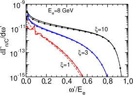
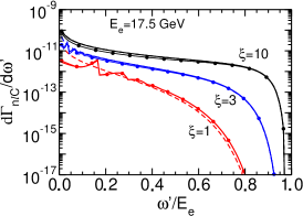
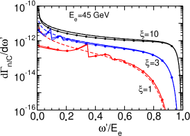
Figure 1: (Color online) The dimensionless differential rate $d\Gamma_{n\ell C}/d\omega^{\prime}$ as a function of $\omega^{\prime}$ (scaled by $E_{e}$) for electron beam energies $E_{e}=8$ GeV (top panel), 17.5 GeV (middle panel) and 45 GeV (bottom panel) at different values of $\xi=1$ (red), 3 (blue) and 10 (black). The solid curves depict the monochromatic model Eqs. (2, 3), while dotted curves use the approximation Eq. (7). Dashed curves are for the approximation Eq. (8). The solid and dotted curves display harmonic structures at low values of $\omega^{\prime}$ and $\xi$.

When considering a laser pulse, instead of the monochromatic background field, an additional scale enters, which characterizes, e.g. the pulse duration. Due to interference effects, the $out$-photon spectra may acquire more complex shapes with nonlinear dependencies on pulse shape and duration. There is extended literature on this and attempts of useful approximation schemes. We emphasize again that, in our positron number estimate below, the rate $\frac{d\Gamma_{n\ell C}(\omega^{\prime}|E_{e})}{d\omega^{\prime}}$ is to be integrated over $\omega^{\prime}$ with the weight $\frac{d\Gamma_{n\ell BW}(E^{+}|\omega^{\prime})}{dE^{+}}$ at given $E^{+}$. In so far, the (fine or harmonic) structures in $\frac{d\Gamma_{n\ell C}(\omega^{\prime}|E_{e})}{d\omega^{\prime}}$ do not matter. The agreement of the differential cross section for a pulse (see figure 8 in Kampfer:2020cbx ) with the monochromatic spectrum according to Eqs. (2, 3) support that claim. As a consequence, Eqs. (2, 3, 7, 8) provide useful ingredients of our n$\ell$C$\otimes$n$\ell$BW folding model.

II.2 Nonlinear Breit-Wheeler process

The differential rate of produced positrons in nonlinear (essentially multi-photon) Breit-Wheeler process $\gamma^{\prime}+{\cal L}\to e^{+}e^{-}$ for given four-momentum $k^{\prime}$ ($in$-photon $\gamma^{\prime}$, frequency $\omega^{\prime}$) and $k$ (laser, frequency $\omega$) reads for head-on collisions Ritus85

$$\frac{d\Gamma_{n\ell BW}}{dE^{+}} = \frac{\alpha m^{2}}{{\omega^{\prime}}^{2}}\sum\limits_{n=n_{\rm min}}^{\infty}{\cal J}_{n}(z,u,\xi),$$ (9)

$${\cal J}_{n}=J_{n}^{2}(z) + \xi^{2}w(u)\left(\left[\frac{n^{2}}{z^{2}}-1\right]J_{n}^{2}(z)+{J_{n}^{\prime}}^{2}(z)\right),$$ (10)

where $E^{+}$ is the positron energy, $w(u)=(2u-1)$ and

$$n_{\rm min} = \left\lceil 1+\frac{m^{2}(1+\xi^{2})\omega^{\prime}}{4\omega E^{+}(\omega^{\prime}-E^{+})}\right\rceil\leavevmode\nobreak\ ,$$ (11)

$$z = \frac{2\xi n}{\sqrt{1+\xi^{2}}}\sqrt{\frac{u}{u_{n}}\left(1-\frac{u}{u_{n}}\right)}\leavevmode\nobreak\ ,$$ (12)

$$u = \frac{{\omega^{\prime}}^{2}}{4E^{+}(\omega^{\prime}-E^{+})}\leavevmode\nobreak\ ,\qquad u_{n}=\frac{n\omega\omega^{\prime}}{m^{2}(1+\xi^{2})}\leavevmode\nobreak\ .$$ (13)

Some approximation is based on Eq. (10) with (7) yielding

$${\cal J}_{n}(z,u,\xi)\approx\frac{1}{2\pi}{\rm e}^{2n(a-\tanh a)}\frac{1+2\xi^{2}(2u-1)\sinh^{2}a}{n\tanh a}.$$ (14)

Analog to Eq. (8) one can utilize the approximation Ritus85

$$\frac{d\Gamma_{n\ell BW}}{dE^{+}}\approx\frac{\alpha m^{2}}{\pi{\omega^{\prime}}^{2}}\left\{\int\limits_{z}^{\infty}dy\,\Phi(y)-\frac{2}{z}(2u-1)\Phi^{\prime}(z)\right\},$$ (15)

with $z=(4u/\chi_{\gamma})^{2/3}$ and $\chi_{\gamma}=\xi k\cdot k^{\prime}/m^{2}$, which both have been employed, e.g. in King:2013osa ; King:2013zw .

The dependence of the rate $d\Gamma_{n\ell BW}/dE^{+}$ as a function of $\omega^{\prime}$ for fixed positron energy $E^{+}=E_{e}/2$ is exhibited in Fig. 2. Since $E^{+}<\omega^{\prime}$, only the range $0.5<\omega^{\prime}/E_{e}$ is accessible. The small (large)-$\omega^{\prime}$ range becomes accessible for small (large) values of $E^{+}$. Note the opposite tendencies of the Compton and Breit-Wheeler rates as a function of $\omega^{\prime}$, making the details of small-$\omega^{\prime}$ and large-$\omega^{\prime}$ distributions irrelevant when considering their product in convoluting them. The laser intensity dependency is also very strong in the considered parameter range.

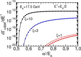
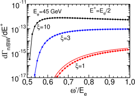
Figure 2: (Color online) The dimensionless differential rate $d\Gamma_{n\ell BW}/dE^{+}$ as a function of $\omega^{\prime}$ (scaled by $E_{e}$) for positron energies $E^{+}=E_{e}/2$ for $E_{e}=8$ GeV (top panel), 17.5 GeV (middle panel) and 45 GeV (bottom panel) at different values of $\xi=1$ (red), 3 (blue) and 10 (black). Results using either Eqs. (9, 10) (solid curves) or (9, 14) (dashed curves) are not distinguishable on the given scale. The approximation (15) is displayed by dotted curves.

Some information on the $E^{+}$ dependence of $d\Gamma_{n\ell BW}/dE^{+}$ at fixed values of $\omega^{\prime}$ is given in the left column of Fig. 3 for $E_{e}=17.5$ GeV at different values $\xi$. The symmetric energy distributions have a pronounced maximum at $E^{+}=\omega^{\prime}/2$ and monotonically decrease for $E^{+}\to 0$ or $E^{+}\to\omega^{\prime}$, thus evidencing the relevant positron energy range. To quantify the positron polar-angular distribution and to characterize the relevant range we exhibit these in the right column of Fig. 3. The angular distributions exhibit a dead cone at small angles $\Theta^{\prime}$ relative to the $\omega^{\prime}$ photon direction, i.e. at $(1-\cos\Theta^{\prime})\to 0$, similar to the nonlinear Compton process HernandezAcosta:2020agu . The dead cone effect becomes sharper with increasing value of $\xi$. The displayed angular-differential rate is determined by

$$\frac{d\Gamma_{n\ell BW}}{d\cos\Theta^{+}}=\frac{\alpha m^{2}}{\omega^{\prime}}\sum\limits_{n=n_{\rm min}}^{\infty}\frac{q^{2}}{|q\omega_{+}^{\prime}-q_{0}\omega_{-}^{\prime}\cos\Theta^{+}|}{\cal J}_{n},$$ (16)

where the definitions (12, 13) apply for $z$ and $u_{n}$ entering ${\cal J}_{n}$ (10) with $\omega_{\pm}^{\prime}=\omega^{\prime}\pm n\omega$, $q=\sqrt{q_{0}^{2}-m^{2}(1+\xi^{2})}$, $q_{0}=A+\sqrt{A^{2}-B}$, as well as

$$n_{min} = \left\lceil 1+\frac{m^{2}(1+\xi^{2})}{\omega\omega^{\prime}}\right\rceil,$$ (17)

$$u = \frac{{\omega^{\prime}}^{2}}{(q_{0}+q\cos\Theta^{+})(2\omega^{\prime}-q_{0}-q\cos\Theta^{+})},$$ (18)

$$A = \frac{2n\omega\omega^{\prime}\omega_{+}^{\prime}}{{\omega_{+}^{\prime}}^{2}-{\omega_{-}^{\prime}}^{2}\cos^{2}\Theta^{+}},$$ (19)

$$B = \frac{m^{2}(1+\xi^{2}){\omega_{-}^{\prime}}^{2}\cos^{2}\Theta^{+}+4(n\omega\omega^{\prime})^{2}}{{\omega_{+}^{\prime}}^{2}-{\omega_{-}^{\prime}}^{2}\cos^{2}\Theta^{+}}.$$ (20)

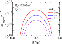
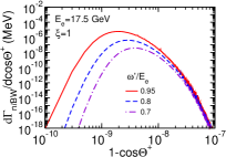
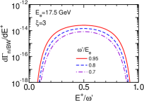
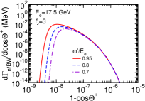
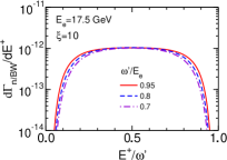
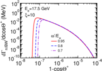
Figure 3: (Color online) Positron production rates $d\Gamma_{n\ell BW}/dE^{+}$ as a function of positron energy $E^{+}$ (scaled by $\omega^{\prime}$) (left row) and $d\Gamma_{n\ell BW}/d\cos\Theta^{+}$ as a function of the positron lab. angle $\Theta^{+}$ relative to the $\omega^{\prime}$-photon direction (right row) at laser intensity parameters $\xi=1$ (top panel), 3 (middle panel) and 10 (bottom panel) and various energies of the probe photon $\omega^{\prime}$ in units of $E_{e}=17.5$ GeV. In calculation we use Eq. (14).

III Estimate of positron production

The above recollected rates for monochromatic background (laser) fields may be realized by a very long flattop section of the envelope. To be specific consider a plane-wave laser model with electromagnetic vector potential $A(\phi)\propto f(\phi)\,cos(\phi)$ with invariant phase $\phi=\omega(t+z)$, i.e. a beam moving along $z$ axis to left, and lines of constant phase are inclined by $45^{\circ}$ in the observer’s space-time ($z$-$t$) diagram. An idealized flattop envelope would be $f(\phi)=\sqcap(\phi,\Delta\phi)$ with $\sqcap=1$ for $\phi\in[0,\Delta\phi]$ and zero elsewhere, i.e. the number of oscillations within the pulse is $N=\Delta\phi/2\pi$. (Such an envelope has been considered in King:2020hsk and Tang:2021qht for n$\ell$C and n$\ell$BW, respectively, with emphasis on the soft part of the distributions and comparison of various approximation schemes.) Despite intricate effects of finite-time laser pulses King:2020hsk , a simplified estimate of the number of produced quanta would be to use the monochromatic rate multiplied by the pulse duration. In such a spirit we estimate the number of produced positrons by convoluting the rate of produced hard photons, emitted by a high-energy electron – traversing a pulse on the trajectory $t\approx z$ near light cone thus crossing the invariant phase lines $\phi=0\cdots\Delta\phi$ – with the rate of positrons produced by these photons later on within the same pulse. Let be the relevant time intervals $T_{C,BW}$ for the respective n$\ell$C and n$\ell$BW processes. Then the energy distribution of positrons in the folding model n$\ell$C $\otimes$ n$\ell$BW may be expressed as

$$\frac{dN^{e^{+}}}{dE^{+}}=\int\limits_{0}^{E_{e}}d\omega^{\prime}\int\limits_{0}^{T_{C}}dt\frac{d\Gamma_{n\ell C}(\omega^{\prime},t)}{d\omega^{\prime}}\int\limits_{t}^{T_{BW}}dt^{\prime}\frac{d\Gamma_{n\ell BW}(\omega^{\prime},t^{\prime})}{dE^{+}},$$ (21)

where $d\Gamma_{n\ell C}(\omega^{\prime},t)/d\omega^{\prime}$ is the rate of photons per frequency interval $d\omega^{\prime}$ emerging from one electron undergoing Compton scattering at time $t\in[0,T_{C}]$, and $d\Gamma_{n\ell BW}(\omega^{\prime},t^{\prime})/{dE^{+}}$ is the the differential rate of Breit-Wheeler pairs generated by a probe photon of frequency $\omega^{\prime}$ at lab. frame time $t^{\prime}\in[t,T_{BW}]$. Formally, $\Gamma_{n\ell C}(\omega^{\prime},t)\to\Gamma_{n\ell C}(\omega^{\prime})\sqcap(t,T_{C})$ and $\Gamma_{n\ell BW}(\omega^{\prime},t^{\prime})\to\Gamma_{n\ell BW}(\omega^{\prime})\sqcap(t^{\prime},T_{BW})$. The above picture of an electron traversing a laser pulse in head-on geometry near to light cone means $T_{C}=T_{BW}\equiv T_{0}=\pi N/\omega$. (The pulse duration for an observer at rest in the $z$-$t$ Minkowski frame is $2T_{0}$. On the trajectory $z\approx t$, the invariant phase is $\phi\approx 2\omega t$, therefore, $\sqcap(t,T_{0})\to\sqcap(\phi,\Delta\phi)$.) Neglecting spatio-temporal variations within the pulse by using Eqs. (2) and (9), our final formula becomes

$$\frac{dN^{e^{+}}}{dE^{+}}=F_{t}\int\limits_{E^{+}}^{E_{e}}d\omega^{\prime}\frac{d\Gamma_{n\ell C}(\omega^{\prime})}{d\omega^{\prime}}\,\frac{d\Gamma_{n\ell BW}(\omega^{\prime},E^{+})}{dE^{+}}\leavevmode\nobreak\ ,$$ (22)

with $F_{t}=N^{e}_{0}\,T_{C}(T_{BW}-T_{C}/2)=T_{0}^{2}/2$, i.e. a quadratic dependence on the pulse length via $N^{2}$. Such an estimate neglects the attenuation of the primary electron beam towards emitting a hard photon at $t\approx z$ (which can be cured by a Glauber eikonal factor), a formation time for separating the recoil electron and the on-shell photon (which is here assumed to continue on the straight trajectory), and the poor approximation of the photon number distribution in a finite pulse by neglecting bandwidth effects (see Appendix A for genuine bandwidth effects in the weak-field trident process). Obviously, the separation in one-step and the here only partially uncovered two-step processes on probabilistic level is rather crude. Therefore, in our estimates we either use $T_{0}=2\pi/\omega$ (see Appendix B for a comparison with E-144 data) and attach to the Compton rate the number $N^{e}_{0}=6\times 10^{9}$ of primary electrons per bunch or scale out the normalization factor $F_{t}$ footnote_in_bibliography .

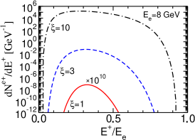
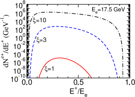
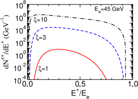
Figure 4: (Color online) The distribution of positrons $dN^{e^{+}}/dE^{+}$ as a function of lab. energy $E^{+}$ at different values of $\xi=1$ (red), 3 (blue dashed) and 10 (black dot-dashed) for electron beam energies $E_{e}=8$ GeV (top panel), 17.5 GeV (middle panel) and 45 GeV (bottom panel) with $N_{0}=6\times 10^{9}$. The harmonic structures of $d\Gamma_{n\ell C}/d\omega^{\prime}$ seen in Fig. 1 at small values of $\omega^{\prime}$ are irrelevant for $dN^{e^{+}}/dE^{+}$ since $d\Gamma_{n\ell BW}/d\omega^{\prime}$ (see Fig. 2) is exceedingly small there.

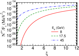
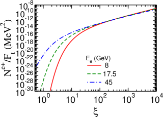
Figure 5: (Color online) The scaled number of positrons $N^{e^{+}}/F_{t}$ as a function of laser intensity parameter $\xi$ for electron beam energies $E_{e}=8$ GeV (solid red), 17.5 GeV (dashed green) and 45 GeV (dot-dashed blue). Top panel: for intensity parameter $\xi$ in the LUXE - FACET-II (E-320) range. Bottom panel: for a large range of $\xi$. Note the value of the above given factor $F_{t}\,\omega^{2}\approx 20\,N_{0}$.

Our estimate of the positron distribution $dN^{e^{+}}/dE^{+}$ is exhibited in Fig. 4. For n$\ell$Co and n$\ell$BW vertices we us Eqs.(8) and (9, 14), respectively. The positron spectra display asymmetric bump-like distributions with the maximum shifted to smaller energies, i.e. to $E^{+}<E_{e}/2$. At large beam-electron energy the bump like distributions become flatter and slightly inclined. The available phase space, $0<E^{+}<E_{e}$, becomes more and more uncovered with increasing values of $\xi$. Note the enormous sensitivity against variations of the laser intensity $\xi$.

To quantify the $\xi$ dependence we display in Fig. 5 the scaled positron number for three electron beam energies. To convert to absolute numbers one has to multiply by the beam electron number per bunch and adjust $T_{C}$ and $T_{BW}$ in Eq. (21) which determine the factor $F_{t}$ in Eq. (22). The top panel is for the laser intensity range to be uncovered by LUXE - E-320. Using the above formalism also for ultra-high intensities, the scaled positron number converge at $\xi>50$ to a unique value irrespective of the electron beam energy $E_{e}$. Such a behavior is consistent with the stabilization phenomenon discussed in Kaminski:2006xlq .

The laser intensity parameter may be noted as $\xi=\frac{m}{\omega}\frac{{\cal E}}{{\cal E}_{crit}}$ with the (critical) Sauter-Schwinger electric field strength ${\cal E}_{crit}=m^{2}/|e|\approx 1.3\times 10^{18}$ V/m. According to Hartin:2018sha , “Measuring the Boiling Point of the Vacuum of Quantum Electrodynamics”, one can perform a deconvolution of data to get an experimental access to ${\cal E}_{crit}$, supposed all other parameter are under control. Given the strong $\xi$ dependence of the individual contributions in n$\ell$C($\xi$) $\otimes$ n$\ell$BW($\xi)$, see Figs. 1 and 2, one can analogously test the dependence of the complete two-step positron number $N^{e^{+}}$ on ${\cal E}_{crit}$. A useful quantity is the ratio $N^{e^{+}}(\epsilon{\cal E}_{crit})/N^{e^{+}}({\cal E}_{crit})=N^{e^{+}}(\xi/\epsilon)/N^{e^{+}}(\xi)$ as a function of $\xi$ with all other kinematic quantities fixed, see Fig. 6. Due to the exponential suppression of both the nonlinear Compton process HernandezAcosta:2020agu and the nonlinear Breit-Wheeler process Ritus85 ; Reiss:1971wf , which is encoded in the strong $\xi$ dependence, such a ratio exhibits in fact a stark sensitivity on variations of $E_{crit}$ on the 10% level.

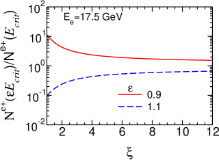
Figure 6: (Color online) The ratio $N^{e^{+}}(\epsilon\,{\cal E}_{crit})/N^{e^{+}}({\cal E}_{crit})$ as a function of $\xi$ for $E_{e}=17.5$ GeV. Upper (lower) curve: $\epsilon=0.9$ (1.1). Both curves approach unity for large values of $\xi$.

IV Summary

In summary we calculate, within a folding model n$\ell$C $\otimes$ n$\ell$BW as approximation of the trident process, the energy distributions of positrons produced in collisions of ultra-relativistic electrons with a high-intensity laser beam for different electron beam energies and intensities of the laser beam. As a prerequisite we evaluate the gross shape (by ignoring the laser pule shape and thus not catching the complex interference pattern) of photon energy distributions from n$\ell$C, which are also experimentally accessible Fleck:2020opg . Our predictions are for parameters motivated by forthcoming experiments with $\xi=1\cdots 10$, in particular at LUXE and FACET-II (E-320). While the employed folding model is related to the two-step part of trident in product approximation, the interesting one-step contribution should manifest itself as deviation. Our model may serve as reference easy to handle in such a search for genuine strong-field QED effects.

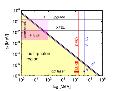
Figure 7: (Color online) Trident landscape over the $\omega$-$E_{e}$ plane. The near-by diagonal lines depict the loci of $\sqrt{s}/m=3.353$, 3.05, 3 and 2.95 (from top to bottom) linear trident processes. The yellow region is below the threshold, i.e. accessible only by multi-photon effects in the nonlinear trident or by bandwidth effects in linear trident. Thin horizontal lines mark 1.5 eV, 15 keV and 150 keV as representatives of optical lasers, XFEL and possible XFEL upgrade. Thin vertical lines bracket the energies of the Europaen XFEL electron driver beam (DESY) and Stanford linear accelerator (SLAC). Boxes filled with color indicate the previous E-144 (blue) and future LUXE (red) experiments as well as possible options at HIBEF (magenta) when using laser accelerated electrons with $E_{e}<100$ MeV.

In future developments one may envisage triple-vertex processes, e.g. irradiating laser-accelerated electrons in the laser focus by a high-energy XFEL beam, $\mbox{XFEL}+(e^{-}+{\cal L})\to{e^{-}}^{\prime}+e^{+}e^{-}$. This XFEL-induced trident is a nonlinear virtual Compton process, which is accessible to the HIBEF collaboration HIBEF , in particular with an upgrade of the European XFEL. (The corresponding theory of the nonlinear real Compton sub-process, $\mbox{XFEL}+(e^{-}+{\cal L})\to{e^{-}}^{\prime}+\gamma^{\prime}$, has been already dealt with in collinear kinematics Seipt:2013hda .) An intermediate configuration could investigate the process $\mbox{XFEL}+e_{{\cal L}}^{-}\to{e^{-}}^{\prime}+e^{+}e^{-}$, again with laser-accelerated electrons ($e_{{\cal L}}^{-}$), but outside the laser focus. Since in the present setting the XFEL intensity parameter $\xi$ is small, $\xi_{\mbox{{\footnotesize XFEL}}}\ll 1$, the multi-photon effects - which are decisive in section III - are negligible. The threshold electron energy is $E_{e}\approx 32$ MeV for $\omega_{\mbox{{\footnotesize XFEL}}}=15$ keV. Even below that value, pair production is enabled by bandwidth effects, see Appendix A. If (by a yet unknown technology) the XFEL beam could be focused to achieve $\xi_{\mbox{{\footnotesize XFEL}}}\gtrsim 1$, a new domain of testing strong-field QED effects would be opened up, see the magenta region in Fig. 7.

Appendix A Bandwidth effects in linear trident

Turning to boost invariant quantities we describe the linearly polarized laser pulse by the electromagnetic four-potential $A=(A^{0},\vec{A})$ in axial gauge, $A^{0}=0$, where $\vec{A}=f(\phi)\,\vec{a}_{x}\,\cos\phi$ and the envelope function reads $f(\phi)=\cos^{2}\left(\frac{\pi\phi}{2\Delta\phi}\right)\sqcap(\phi,2\Delta\phi)$, i.e. the number of laser-field oscillations within the pulse is $N=\Delta\phi/\pi$. The invariant laser phase is $\phi=k\cdot x$. Due to the finite pulse duration bandwidth effects occur, since the power spectrum of the laser has frequency components $\lessgtr\omega$, thus enabling the sub-threshold pair production in the process $\mbox{XFEL}+e^{-}\to{e^{-}}^{\prime}+e^{+}e^{-}$. The here assumed laser intensity parameter $\xi=e^{2}{\vec{a}\,}^{2}/m^{2}\ll 1$ is too small to allow for genuine multi-photon effects.

In Fig. 8 the inclusive differential positron cross section $d^{3}\sigma/dy\,dp_{\perp}\,d\varphi$ is exhibited, where $y$, $p_{\perp}$ and $\varphi$ denote the rapidity, the transverse momentum and azimuthal angle (w.r.t. to the polarization direction given by $\vec{a}_{x}$) of the produced positrons. The presented results are based on the weak-field evaluation of the l.h.s. Furry picture diagrams displayed in the introduction. We have selected three energies described by the Mandelstam variable $s=(p+k)^{2}$. The threshold is given by $\sqrt{s}=3m$. The left and middle panels are above and near threshold, while the right panel is below the threshold. The shorter the pulse, i.e. the smaller $\Delta\phi$, the wider becomes the kinematically accessible region. In the limit of long pulses, $\Delta\phi\gg 1$, the sub-threshold production is strongly suppressed.

The figure applies to any position on the respective diagonal lines in Fig. 7 for given value of $\sqrt{s}$ by shifting the rapidity $y\to y+y_{x}$ with $y_{x}=\ln\sqrt{s}/m$. The positron energy in the lab. frame, where $E_{e}=m\cosh y_{e}$, is $E^{+}=\sqrt{m^{2}+{p_{\perp}}^{2}}\cosh(y+y_{x}+y_{e})$.

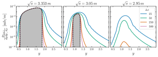
Figure 8: (Color online) Inclusive differential positron cross section $d^{3}\sigma/dy\,dp_{\perp}\,d\varphi$ for $\sqrt{s}/m=3.353$ (left panel), 3.05 (middle panel) and 2.95 (right panel) as a function of rapidity $y$ for $p_{\perp}/m=0.15$ and $\varphi=0$. The pulse duration parameter is $\Delta\phi=25$ (blue), 50 (green), 250 (red) and 500 (magenta). The black dashed curves limiting the gray region in left and middle panels depict the case of a monochromatic beam, i.e. $\Delta\phi\to\infty$. Details of the employed formalism and the kinematic relations can be found in HernandezAcosta:2019vok ; UHA .

Appendix B Testing EQ.(22) BY E-144 DATA

The choice $F_{t}=T_{0}^{2}/2$ with $T_{0}=2\pi/\omega$ in Eq. (22) copes well with the $\xi$ dependence of E-144 data (see Fig. 9). Also the differential $E^{+}$ dependence is sensitive to variations of $\xi$ (see Fig. 10). An effective value of $\xi=0.25$ is consistent with the positron momentum distribution of E-144 (see Fig. 11).

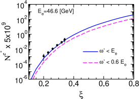
Figure 9: (Color online) Positron number as a function of laser intensity parameter $\xi$ for $F_{t}=T_{0}^{2}/2$ with $T_{0}=2\pi/\omega$ and $5\times 10^{9}$ electrons per bunch in Eq. (22). The data are from Bamber:1999zt (table 13). Accordingly the here employed laser frequency is $\omega=2.3527$ eV.

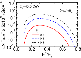
Figure 10: (Color online) Differential positron spectrum $dN^{e^{+}}/dE^{+}$ as a function of $E^{+}/E_{e}$ with the same normalization as in Fig. 9 for $\xi=0.2$ (red), 0.3 (blue dashed) and 0.4 (black dot-dashed). Despite the employed head-on geometry a value of $\xi=0.246$ reproduces the peak height of Mackenroth:2018smh (see figure 2 there) when imposing the multiplicative factor of $2\times 10^{4}$ for the number of laser shots; our distribution is up shifted by about 2 GeV and has a somewhat steeper l.h.s. flank.

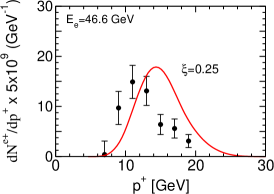
Figure 11: (Color online) Differential positron spectrum $dN^{e^{+}}/dp^{+}$ (red curve) as a function of the lab. positron momentum $p^{+}$ with the same normalization as in Figs. 9 and 10 for $\xi=0.25$ (see also Hu:2010ye ) and for 21,962 laser shots. Data from Bamber:1999zt (table 12). Including an inclination of $17^{\circ}$ between electron beam and laser beam shifts the red curve to left.