Online Stochastic Optimization for Unknown Linear Systems: Data-Driven Synthesis and Controller Analysis

Abstract

This paper proposes a data-driven control framework to regulate an unknown, stochastic linear dynamical system to the solution of a (stochastic) convex optimization problem. Despite the centrality of this problem, most of the available methods critically rely on a precise knowledge of the system dynamics (thus requiring off-line system identification and model refinement). To this aim, in this paper we first show that the steady-state transfer function of a linear system can be computed directly from control experiments, bypassing explicit model identification. Then, we leverage the estimated transfer function to design a controller – which is inspired by stochastic gradient descent methods – that regulates the system to the solution of the prescribed optimization problem. A distinguishing feature of our methods is that they do not require any knowledge of the system dynamics, disturbance terms, or their distributions. Our technical analysis combines concepts and tools from behavioral system theory, stochastic optimization with decision-dependent distributions, and stability analysis. We illustrate the applicability of the framework on a case study for mobility-on-demand ride service scheduling in Manhattan, NY.

I Introduction

This paper focuses on the design of output feedback controllers to regulate the inputs and outputs of a discrete-time linear time-invariant system to the solution of a convex optimization problem. Our controller synthesis is inspired by principled optimization methods, properly modified to account for output feedback from the dynamical system (similarly to [2, 3, 4, 5, 6, 7, 8, 9]). These problems are relevant in application domains such as power grids [10, 4], transportation systems [7], robotics [8], and control of epidemics [11], where the target optimization problem encodes desired performance objectives and constraints (possibly dynamic and time-varying) of the system at equilibrium. Within this broad context, we propose a new approach for the synthesis of data-driven feedback controllers for unknown stochastic LTI dynamical systems, and we consider the case where the system is driven towards optimal solutions of a stochastic optimization problem.

Most of the recent literature on online optimization for dynamical systems critically relies on the assumption that the system dynamics are known [2, 3, 4, 6, 7, 12, 9]. Unfortunately, perfect system knowledge is rarely available in practice – especially when exogenous disturbances are not observable and/or inputs are not persistently exciting – because maintaining and refining full system model often requires ad-hoc system-identification phases. In lieu of system-based controller synthesis, data-driven controllers can be fully synthesized by leveraging data from past trajectories. To the best of our knowledge, the design of optimization-based controllers that bypass model identification is still lacking in the literature.

Related Work. Data-driven control methods exploit the ability to express the trajectories of a linear system in terms of a sufficiently-rich single trajectory, as shown by the fundamental lemma [13]. This result, developed in the context of the behavioral framework, has enabled the synthesis of several types of controllers, including static feedback controllers [14, 15, 16], model predictive controllers [17, 18], minimum-energy control laws [19], to solve trajectory tracking problems [20], distributed control problems [21], and recent extensions account for systems with nonlinear dynamics [22, 23].

The line of research on online convex optimization [24] is also related to this work. Several works applied online convex optimization to control plants modeled as algebraic maps [25, 26, 27] (corresponding to cases where the dynamics are infinitely fast). When the dynamics are non-negligible, LTI systems are considered in [4, 10, 7, 5], stable nonlinear systems in [6, 28], switching systems in [12], and distributed multi-agent systems in [29, 3]. All these works consider continuous-time dynamics and deterministic optimization problems, and derive results in terms of asymptotic or exponential stability. In contrast, here we focus on discrete-time stochastic LTI systems and stochastic optimization problems. Discrete dynamics were the focus of [8], which is however limited to absence of disturbances. Data-driven implementations of online optimization controllers have not been explored yet. A notable exception is [30], which however does not account for the presence of noise, and results are limited to regret analysis. In contrast, when the disturbance terms are unknown, the distributions of the random variables that characterize the cost are parametrized by the decision variables, thus leading to a stochastic optimization problem with decision-dependent distributions, as studied in [31, 32, 33]. In this work, we build upon this class of problems, but accounting for two additional complexities: the online nature of the optimization method and the coupling with a dynamical system.

Contributions. The contribution of this work is fourfold. First, we show that the (steady-state) transfer function of a linear system can be computed from (non steady-state), finite-length input-output trajectories generated by the open-loop dynamics, without any knowledge or estimation of the system parameters. Second, we demonstrate that when the system is affected by unknown disturbances terms, the proposed data-driven framework can still be used to determine an approximate transfer function and, in this case, we explicitly characterize the approximation error. A distinctive feature of our framework, and in contrast with [34, 35, 36, 20], is that we account for the presence of disturbances affecting both the output equation and the model equation. Third, we leverage this data-driven representation to propose a control method to regulate the system to an equilibrium point that is the solution of a stochastic optimization problem. Our design approach is inspired by an online version of the stochastic projected gradient-descent algorithm [37]. One fundamental challenge in the design of the controller is that an error in the estimated transfer function leads to a stochastic optimization problem with decision-dependent distribution [33], that is, the optimization variable induces a shift in the distribution of the underlying random variables that parametrize the cost. This is a class of problems whose direct solution is intractable in general [31]. To bypass this hurdle, we leverage the notion of stable optimizer [31, 32], and we develop a stochastic controller that regulates the system towards such optimizer, up to an asymptotic error that depends on the time-variability of the optimization problem. We show that the controller exhibits strict contractivity with respect to the stable optimizers in expectation, and we explicitly quantify its transient performance. Fourth, we study a real-time fleet management problem, where a ride service provider seeks to maximize its profit by dispatching its fleet while serving ride requests from its customers. We demonstrate the applicability and benefits of our methods numerically on a real network and demand data.

This paper generalizes the preliminary work [1] in several directions. First, we focus on optimization problems that are stochastic rather than deterministic. This fact raises new challenges in the development of optimization methods that account for decision-dependent distributions. Second, we account for the presence of disturbances in the training data. As an additional contribution, our treatment only requires the system to be observable, instead of relying on direct state measurements. Fourth, we provide explicit (exponential) contraction bounds for the proposed control methods. Finally, here we illustrate the applicability of the methods to a ride-service scheduling problem for mobility-on-demand management.

Organization. The paper is organized as follows. Section II presents some basic notions used in our work, in Section III we formalize the problem of interest, Section IV illustrates our controller synthesis method, in Section V we discuss data-driven techniques to compute transfer function of linear systems, and Section VI presents the controller analysis. Section VII illustrates an application of the method to ride service scheduling and Section VIII concludes the paper.

II Preliminaries

In this section, we outline the notation and introduce some preliminary concepts used throughout the paper.

Notation. Given a symmetric matrix $M\in{}^{n\times n}$, $\underline{\lambda}(M)$ and $\bar{\lambda}(M)$ denote its smallest and largest eigenvalue, respectively; $M\succ 0$ indicates that $M$ is positive definite and $\|M\|_{F}$ denotes the Frobenius norm. For a vector $u\in{}^{n}$, we denote $\|u\|$ the Euclidean norm of $u$ and by $u^{\top}$ its transpose. For vectors $u\in{}^{n},w\in{}^{m}$, we use the short-hand notation $(u,w)\in{}^{n+m}$ for their vector concatenation, i.e., $(u^{\top},w^{\top})^{\top}$.

Persistency of Excitation. We next recall some useful facts on behavioral system theory from [13]. For a signal $k\mapsto z_{k}\in{}^{\sigma}$, $k\in\mathbb{Z}$, we denote the vectorization of $z$ restricted to the interval $[k,k+T]$, $T\in\mathbb{Z}_{\geq 0}$, by

$$z_{[k,k+T]}=(z_{k},\dots,z_{k+T}).$$

Given $z_{[0,T-1]}$, $t\leq T$, and $q\leq T-t+1$, we let $Z_{t,q}$ denote the Hankel matrix of length $t$ associated with $z_{[0,T-1]}$:

$$Z_{t,q}=\begin{bmatrix}z_{0}&z_{1}&\ldots&z_{q-1}\\ z_{1}&z_{2}&\ldots&z_{q}\\ \vdots&\vdots&\ddots&\vdots\\ z_{t-1}&z_{t}&\ldots&z_{q+t-2}\end{bmatrix}\in{}^{\sigma t\times q}.$$

Moreover, we use $[Z_{t,q}]_{i}$, $i\in\{1,\dots,t\}$ to denote the $i$-th block-row of $Z_{t,q}$, namely, $[Z_{t,q}]_{i}=[z_{i-1},~{}z_{i},~{}\dots,~{}z_{i+q-2}]$.

Definition II.1

(Persistently Exciting Signal [13]) The signal $z_{[0,T-1]}$, $z_{k}\in{}^{\sigma}$ for all $k\in\{0,\dots,T-1\}$, is persistently exciting of order $t$ if $Z_{t,q}$ has full row rank $\sigma t$. $\square$

We note that persistence of excitation implicitly requires $q\geq\sigma t$ (which in turns requires $T\geq(\sigma+1)t-1$).

Consider the linear dynamical system

$$x_{k+1} =Ax_{k}+Bu_{k}, y_{k} =Cx_{k}+Du_{k},$$ (1)

with $x\in{}^{n}$, $u\in{}^{m}$, $A\in{}^{n\times n}$, $B\in{}^{n\times m}$, $C\in{}^{p\times n}$, $D\in{}^{p\times m}$. Let $\mathcal{C}_{\theta}:=[B,AB,A^{2}B,\dots,A^{\theta-1}B]$ and $\mathcal{O}_{\nu}:=[C^{\mathsf{T}},A^{\mathsf{T}}C^{\mathsf{T}},\dots,(A^{\mathsf{T}})^{\nu-1}C^{\mathsf{T}}]^{\mathsf{T}}$ denote the controllability and observability matrices of (1), respectively. The system is controllable if $\operatorname{rank}(\mathcal{C}_{\theta})=n$ for some $\theta\in\mathbb{Z}_{\geq 0}$, and it is observable if $\operatorname{rank}(\mathcal{O}_{\nu})=n$ for some $\nu\in\mathbb{Z}_{\geq 0}$. The smallest integers $\mu,\nu,$ that satisfy the above conditions are the controllability and observability indices, respectively. We recall the following properties of (1) when its inputs are persistently exciting.

Lemma II.2

(Fundamental Lemma [13, Corollary 2]) Assume (1) is controllable, let $(u_{[0,T-1]},y_{[0,T-1]})$, $T\in\mathbb{Z}_{>0}$, be an input-output trajectory of (2). If $u_{[0,T-1]}$ is persistently exciting of order $n+L$, then:

$$\operatorname{rank}\begin{bmatrix}U_{L,q}\\ X_{1,q}\end{bmatrix}=Lm+n,$$

where $U_{L,q}$ and $X_{1,q}$ denote the Hankel matrices associated with $u_{[0,T-1]}$ and $x_{[0,T-1]}$, respectively. $\Box$

Lemma II.3

(Data characterizes Full Behavior [13, Theorem 1]) Assume (1) is controllable and observable, let $(u_{[0,T-1]},y_{[0,T-1]})$, $T\in\mathbb{Z}_{>0}$, be an input-output trajectory of (2). If $u_{[0,T-1]}$ is persistently exciting of order $n+L$, then any pair of $L$-long signals $(\tilde{u}_{[0,L-1]},\tilde{y}_{[0,L-1]})$ is an input-output trajectory of (2) if and only if there exists $\alpha\in{}^{q}$ such that

$$\begin{bmatrix}\tilde{u}_{[0,L-1]}\\ \tilde{y}_{[0,L-1]}\end{bmatrix}=\begin{bmatrix}U_{L,q}\\ Y_{L,q}\end{bmatrix}\alpha,$$

where $U_{L,q}$ and $Y_{L,q}$ denote the Hankel matrices associated with $u_{[0,T-1]}$ and $y_{[0,T-1]}$, respectively. $\Box$

In words, persistently exciting signals generate output trajectories that can be used to express any other trajectory.

Probability Theory. Let $(\Omega,\mathcal{F},P)$ be a probability space and $z$ be a random variable mapping this space to $({}^{d},B_{\sigma}({}^{m}))$, where $B_{\sigma}({}^{d})$ is the Borel $\sigma$-algebra on ^d. Let $\mathcal{P}$ be the distribution of $z$ and $\Xi\subseteq{}^{m}$ be the support of $\mathcal{P}$. We use $z\sim\mathcal{P}$ to denote that $z$ is distributed according to $\mathcal{P}$, and $\mathbb{E}_{z\text{$\sim$}\mathcal{P}}[\cdot]$ to denote the expectation under $\mathcal{P}$. Let $\mathcal{M}(\Xi)$ be the space of all probability distributions supported on $\Xi$ with finite first moment, i.e., $\mathbb{E}_{z\sim\mathcal{P}}[\|z\|]=\int_{\Xi}\|z\|\mathcal{P}(dz)<\infty$ for all $\mathcal{P}\in\mathcal{M}(\Xi)$. The Wasserstein-1 metric is:

$$W_{1}(\mathcal{P}_{1},\mathcal{P}_{2}):=\inf_{\Pi\in\mathcal{H}(P_{1},P_{2})}\left\{\int_{\Xi^{2}}\|z_{1}-z_{2}\|\Pi(dz_{1},dz_{2})\right\},$$

where $\mathcal{H}(P_{1},P_{2})$ is the set of all joint distributions with marginals $\mathcal{P}_{1}$ and $\mathcal{P}_{2}$. By interpreting the decision function $\Pi$ as a transportation plan for moving a mass distribution described by $\mathcal{P}_{1}$ to another one described by $\mathcal{P}_{2}$, the Wasserstein distance $W_{1}(\mathcal{P}_{1},\mathcal{P}_{2})$ represents the cost of an optimal mass transportation plan, where the transportation costs is described by the 1-Euclidean norm.

Theorem II.4

(Kantorovich-Rubinstein, [38]) For any pair of distributions $\mathcal{P}_{1},\mathcal{P}_{2}\in\mathcal{M}(\Xi)$, the following holds

$$W_{1}(\mathcal{P}_{1},\mathcal{P}_{2})=\sup_{g\in\mathcal{L}_{1}}\left\{\mathbb{E}_{z_{1}\text{$\sim$}\mathcal{P}_{1}}\left[g(z_{1})\right]-\mathbb{E}_{z_{2}\text{$\sim$}\mathcal{P}_{2}}\left[g(z_{2})\right]\right\},$$

where $\mathcal{L}_{1}$ denotes the space of all $1$-Lipschitz functions, i.e.,

$$\mathcal{L}_{1}:=\{g:\Xi\rightarrow{}^{m}\;:\;\|g(z_{1})-g(z_{2})\|\leq\|z_{1}-z_{2}\|\}.$$

The following result is instrumental for our analysis. We provide a short proof for completeness.

Lemma II.5

(Deviation Between Expectations [31, Lemma C.4]) Let $f:{}^{n}\rightarrow{}^{d}$ be $L$-Lipschitz continuous. Then, for any pair of distributions $\mathcal{P}_{1},\mathcal{P}_{2}\in\mathcal{M}(\Xi)$,

$$\|\mathbb{E}_{z_{1}\text{$\sim$}\mathcal{P}_{1}}\left[f(z_{1})\right]-\mathbb{E}_{z_{2}\text{$\sim$}\mathcal{P}_{2}}\left[f(z_{2})\right]\|\leq LW_{1}(\mathcal{P}_{1},\mathcal{P}_{2}).$$

Proof:

Let $v\in{}^{d}$ be any unit vector and let $g(z):=v^{\mathsf{T}}f(z)$. By assumption, $g(z)$ is $L$-Lipschitz continuous and therefore:

$$v^{\mathsf{T}}( \mathbb{E}_{z_{1}\text{$\sim$}\mathcal{P}_{1}}\left[f(z_{1})\right]-\mathbb{E}_{z_{2}\text{$\sim$}\mathcal{P}_{2}}\left[f(z_{2})\right])$$

$$\quad\quad=\mathbb{E}_{z_{1}\text{$\sim$}\mathcal{P}_{1}}\left[v^{\mathsf{T}}f(z_{1})\right]-\mathbb{E}_{z_{2}\text{$\sim$}\mathcal{P}_{2}}\left[v^{\mathsf{T}}f(z_{2})\right])$$

$$\quad\quad=\mathbb{E}_{z\text{$\sim$}\mathcal{Z}(\alpha)}\left[g(z)\right]-\mathbb{E}_{z\text{$\sim$}\mathcal{Z}(\beta)}\left[g(z)\right]\leq LW_{1}(\alpha,\beta),$$

where the last inequality follows by application of Theorem II.4. The result then follows by choosing

$$v=\frac{\mathbb{E}_{z_{1}\text{$\sim$}\mathcal{P}_{1}}\left[f(z_{1})\right]-\mathbb{E}_{z_{2}\text{$\sim$}\mathcal{P}_{2}}\left[f(z_{2})\right]}{\|\mathbb{E}_{z_{1}\text{$\sim$}\mathcal{P}_{1}}\left[f(z_{1})\right]-\mathbb{E}_{z_{2}\text{$\sim$}\mathcal{P}_{2}}\left[f(z_{2})\right]\|}.$$

∎

III Problem Formulation

In this section, we present the problem that is the focus of this work and we discuss a tractable reformulation used for our controller synthesis.

III-A Steady-State Regulation Problem for Linear Systems

We consider discrete-time systems with linear dynamics:

$$x_{k+1} =Ax_{k}+Bu_{k}+Ew_{k}, y_{k} =Cx_{k}+Dw_{k},$$ (2)

where $k\in\mathbb{Z}_{\geq 0}$ is the time index, $x_{k}\in{}^{n}$ is the state, $u_{k}\in{}^{m}$ denotes the control decision at time $k$, $w_{k}\in{}^{r}$ is an unknown exogenous stochastic disturbance with unknown distribution $w_{k}\sim\mathcal{W}_{k}$, and $y_{k}\in{}^{p}$ is the measurable output. We make the following assumptions on (2).

Assumption 1

(System Properties) The system (2) is controllable and observable. Moreover, the matrix $A$ is Schur stable, i.e., for any $Q\succ 0$, there exists $P\succ 0$ such that $A^{\mathsf{T}}PA-P=-Q$.  $\square$

Our control objective is to regulate (2) to the solutions of the following steady-state optimization problem at every time $k$:

$$(u^{*}_{k},x_{k}^{*},y_{k}^{*})\in\arg\min_{\bar{u},\bar{x},\bar{y}}\;\;\; \mathbb{E}_{w_{k}\text{$\sim$}\mathcal{W}_{k}}\left[\phi(\bar{u},\bar{y})\right]$$ (3a)

s.t. $$\bar{x}=A\bar{x}+B\bar{u}+Ew_{k},$$ (3b)

$$\bar{y}=C\bar{x}+Dw_{k},$$ (3c)

where $\phi:{}^{m}\times{}^{p}\rightarrow\real$ denotes a cost function that models losses associated with the control inputs and system outputs. Problem (3) formalizes an equilibrium-selection problem, where the objective is to select an optimal input-state-output triple $(u^{*}_{k},x_{k}^{*},y_{k}^{*})$ that minimizes the expected cost specified by $\phi$. We note that the optimization is time-varying because the distribution of $w_{k}$ is time-varying.

Remark 1

(Relationship with Classical Output Regulation Problem) We note that although (3) formalizes an optimal regulation problem with steady-state constraints similar to the well-established output-regulation problems [39], with respect to the classical framework in our setting the optimal trajectories are not generated by an exosystems (i.e., a known autonomous linear model) but instead are specified as the solution of an optimization problem. $\square$

We impose the following regularity assumptions on $\phi(u,y)$.

Assumption 2

​(Lipschitz and Convexity of Cost Function)​

1. For any fixed $u\in{}^{m}$, the map $y\mapsto\phi(u,y)$ is $\ell$-Lipschitz continuous.

2. For any fixed $y\in{}^{p}$, the map $u\mapsto\nabla\phi(u,y)$ is $\ell_{u}^{\nabla}$-Lipschitz continuous, and for any fixed $u\in{}^{m}$ the map $y\mapsto\nabla\phi(u,y)$ is $\ell_{y}^{\nabla}$-Lipschitz continuous.

3. For any fixed $y\in{}^{p}$, the map $u\mapsto\phi(u,y)$ is $\mu$-strongly convex, i.e., there exists $\mu\in{}_{>0}$ such that, for all $u,u^{\prime}\in{}^{m}$, $\phi(u,y)\geq\phi(u^{\prime},y)+\nabla\phi(u^{\prime},y)^{\mathsf{T}}((u,y)-(u^{\prime},y))+\frac{\mu}{2}\|u-u^{\prime}\|$. $\square$

Strong convexity and Lipschitz-type assumptions impose basic conditions on the growth of the cost function often used for the analysis of first-order optimization methods [40]. Under strong convexity, the function $\phi$ admits a unique critical point $(u^{*}_{k},y_{k}^{*})$ that is also a global optimizer (see e.g. [41]). Notice that, under Assumption 1, $x_{k}^{*}=(A-I)^{\scalebox{0.75}[0.9]{$-$}1}(Bu_{k}^{*}+Ew_{k})$ is also unique since the linear map $(A-I)^{\scalebox{0.75}[0.9]{$-$}1}$ has an empty null space. Hence, in what follows we use $(u^{*}_{k},x_{k}^{*},y_{k}^{*})$ to denote the unique solution of (3). We formalize the problem that is the focus of this work next.

Problem 1

Design an output-feedback controller of the form $u_{k+1}=\mathcal{C}(u_{k},y_{k})$ such that, without any prior knowledge of the matrices $(A,B,C,D,E)$ as well as of the noise distributions $\mathcal{W}_{k}$, the input and output of (2) converge asymptotically to the time-varying optimizer of (3). $\square$

III-B Problem Reformulation for Unknown Dynamics

Since the optimization problem (3) contains only equality constraints, Assumption 1 can be used to recast it as an unconstrained optimization problem, as described next. For any fixed $u\in{}^{m}$ and $w\in{}^{r}$, Assumption 1 guarantees that (2) has a unique exponentially-stable equilibrium point $x=(I-A)^{\scalebox{0.75}[0.9]{$-$}1}(Bu+Ew)$. At the equilibrium, the dependence between system inputs and outputs is given by

$$y=\underbrace{C(I-A)^{\scalebox{0.75}[0.9]{$-$}1}B}_{:=G}u+\underbrace{(D+C(I-A)^{\scalebox{0.75}[0.9]{$-$}1}E)}_{:=H}w.$$ (4)

By using the above representation, (3) can be rewritten as:

$$u_{k}^{*}=\arg\min_{\bar{u}}\;\;\; \mathbb{E}_{w_{k}\text{$\sim$}\mathcal{W}_{k}}\left[\phi(\bar{u},G\bar{u}+Hw_{k})\right].$$ (5)

Next, we observe that the optimization problem (5) is parametrized by the matrix $G$ as well as by the term $Hw_{k}$, which are not known when the system dynamics (2) are unknown. When an approximation $\hat{G}$ of $G$ is available, the optimization problem (5) can be equivalently rewritten as:

$$u_{k}^{*}=\arg\min_{\bar{u}}\;\;\; \mathbb{E}_{\bar{z}\text{$\sim$}\mathcal{Z}_{k}(\bar{u})}\left[\phi(\bar{u},\hat{G}\bar{u}+\bar{z})\right],$$ (6)

where $\bar{z}:=(G-\hat{G})\bar{u}+Hw_{k}$ is a random variable that encodes the lack of knowledge of the map $G$ as well as of the term $Hw_{k}$. We note that the distribution of $\bar{z}$ is parametrized by the decision variable $\bar{u}$ and, in order to emphasize such dependency, in what follows we use the notation $\bar{z}\sim\mathcal{Z}_{k}(\bar{u})$. From an optimization perspective, seeking a solution of (6) raises three main challenges:

1. Because the distribution of $\bar{z}$ is parametrized by the decision variable $\bar{u}$, the resulting cost function is nonlinear in $\bar{u}$, thus making the optimization problem (6) intractable for general costs (even when $u\mapsto\phi(u,z)$ is convex).

2. Since the distribution of the disturbance $w_{k}$ is unknown, the distribution $\mathcal{Z}_{k}(\bar{u})$ is also unknown for any $\bar{u}$. Instead, we only have access to evaluations of the random variable $\bar{z}$ via measurements of the output $y_{k}$ of the system (2). This fact calls for the development of control methods that can adjust the input $u_{k}$ based on noisy evaluations of the cost function through access to the system output $y_{k}$.

3. The closed-form expression for $G$ depends on the system matrices $(A,B,C)$ (cf. (4)), which are unknown. This raises the question of how to construct an approximate map $\hat{G}$ and how to quantify the approximation error.

The subsequent sections address the above challenges. Precisely, (Ch1) is addressed in Section IV.A, while in Section IV.B we propose a control method to address (Ch2). Section IV illustrates a data-driven technique to tackle (Ch3), while Section VI combines the methods by analyzing the performance of the control technique.

IV Synthesis of Online Optimization Controllers for Unknown Linear Systems

In this section, we tackle challenge (Ch1) and we show that the optimization problem (6) can be regarded as a standard stochastic optimization problem by accounting for worst-case shifts in the distribution. Moreover, we use techniques from online optimization to address challenge (Ch2).

IV-A Notion of Stable Optimizer

Because of the direct dependence between the random variable $\bar{z}$ and the decision variable $\bar{u}$ in (6), explicit solution of the optimization problem (6) are out of reach in general. For this reason, we focus on the problem of making online control decisions $u_{k}$ such that, when $u_{k}$ is applied as an input to (2), the resulting cost is optimal for the distribution induced on the random variable $\bar{z}$. This concept is formalized in the following definition, inspired by [31].

Definition IV.1

(Stable Optimizer) The vector ${u}^{\textup{so}}_{k}\in{}^{m}$ is a stable optimizer of (6) at time $k\in\mathbb{Z}_{\geq 0}$ if:

$${u}^{\textup{so}}_{k}=\arg\min_{\bar{u}}\;\;\; \mathbb{E}_{\mathcal{Z}_{k}({u}^{\textup{so}}_{k})}\left[\phi(\bar{u},\hat{G}\bar{u}+\bar{z})\right].$$ (7)

Accordingly, we let ${x}^{\textup{so}}_{k}:=(I-A)^{\scalebox{0.75}[0.9]{$-$}1}(B{u}^{\textup{so}}_{k}+Ew_{k})$. $\square$

In words, ${u}^{\textup{so}}_{k}$ is a stable optimizer if it solves the optimization problem that originates by fixing the distribution of $\bar{z}$ to $\mathcal{Z}_{k}({u}^{\textup{so}}_{k})$. Accounting for stable optimizers allows us to make the optimization problem (6) tractable, since standard gradient-descent methods can be adapted to converge to ${u}^{\textup{so}}_{k}$ (as we show in Section VI). Moreover, convergence to a stable optimizer is desirable because it guarantees that ${u}^{\textup{so}}_{k}$ is optimal for the distribution that it induces. Stable optimizers, in general, may not coincide with the optimizers of (6), and their existence and uniqueness is guaranteed under suitable technical assumptions (see Theorem VI.1). However, an explicit error bound can be derived under suitable smoothness assumptions, as shown next.

Proposition IV.2

(Optimizer Gap) Let Assumption 2 be satisfied, let $u_{k}^{*}$ be the optimizer of (6), and let ${u}^{\textup{so}}_{k}$ be a stable optimizer as defined in (7). Then,

$$\|u_{k}^{*}-{u}^{\textup{so}}_{k}\|\leq\frac{2\ell\|G-\hat{G}\|}{\mu{\sigma}_{\textup{min}}^{2}(\hat{G})},$$ (8)

where ${\sigma}_{\textup{min}}^{2}(\hat{G})$ denotes the smallest singular value of $\hat{G}$.

Proof:

The proof idea is similar to [31, Theorem 4.3]. By recalling that $\bar{z}=(G-\hat{G})\bar{u}+w_{k}$, a direct application of Theorem II.4 yields:

$$W_{1}(\mathcal{Z}_{k}(u),\mathcal{Z}_{k}(u^{\prime}))\leq\|G-\hat{G}\|\|u-u^{\prime}\|,$$ (9)

for any $u,u^{\prime}\in{}^{m}.$ Next, we denote in compact form $f(u,z):=\phi(u,\hat{G}u+z)$. By recalling the definition of $u_{k}^{*}$ and of ${u}^{\textup{so}}_{k}$, we have that $\mathbb{E}_{\mathcal{Z}(u^{*}_{k})}f(u^{*}_{k},z)\leq\mathbb{E}_{\mathcal{Z}({u}^{\textup{so}}_{k})}f({u}^{\textup{so}}_{k},z)$, which implies:

$$\mathbb{E}_{\mathcal{Z}({u}^{\textup{so}}_{k})}\left[f(u^{*}_{k},z)\right] -\mathbb{E}_{\mathcal{Z}({u}^{\textup{so}}_{k})}\left[f({u}^{\textup{so}}_{k},z)\right]$$ (10)

$$\quad\quad\leq\mathbb{E}_{\mathcal{Z}({u}^{\textup{so}}_{k})}\left[f(u^{*}_{k},z)\right]-\mathbb{E}_{\mathcal{Z}(u^{*}_{k})}\left[f(u^{*}_{k})\right].$$

First, we upper bound the right hand side of (10). To this aim, by combining (9) with Assumption 2(a) and by application of Lemma II.5 we have:

$$\mathbb{E}_{\mathcal{Z}({u}^{\textup{so}}_{k})}\left[f(u^{*}_{k},z)\right]-\mathbb{E}_{\mathcal{Z}(u^{*}_{k})}\left[f(u^{*}_{k},z)\right]\leq\ell\|G-\hat{G}\|\|u^{*}_{k}-{u}^{\textup{so}}_{k}\|.$$ (11)

Second, we lower bound the left hand side of (10). To this aim, we note that Assumption 2(c) implies: $f(u^{*}_{k},z)\geq f({u}^{\textup{so}}_{k},z)+\nabla_{u}f({u}^{\textup{so}}_{k},z)^{\mathsf{T}}(u^{*}_{k}-{u}^{\textup{so}}_{k})+\frac{\mu{\sigma}_{\textup{min}}^{2}(\hat{G})}{2}\|u^{*}_{k}-{u}^{\textup{so}}_{k}\|^{2}$ for all $z$. Moreover, since ${u}^{\textup{so}}_{k}$ is a stable optimizer, it satisfies the following variational inequality: $\mathbb{E}_{\mathcal{Z}({u}^{\textup{so}}_{k})}{[\nabla_{u}f({u}^{\textup{so}}_{k},z)^{\mathsf{T}}(u^{\prime}-{u}^{\textup{so}}_{k})]}\geq 0$ for all $u^{\prime}\in{}^{m}$. By combining the above two conditions we obtain:

$$\mathbb{E}_{\mathcal{Z}({u}^{\textup{so}}_{k})}\left[f(u^{*}_{k},z)\right] -\mathbb{E}_{\mathcal{Z}({u}^{\textup{so}}_{k})}\left[f({u}^{\textup{so}}_{k},z)\right]\geq\frac{\mu{\sigma}_{\textup{min}}^{2}(\hat{G})}{2}\|{u}^{\textup{so}}_{k}-u^{*}_{k}\|^{2}.$$ (12)

Finally, the claim follows by combining (11) with (12). ∎

Proposition IV.2 quantifies the error between a stable optimizer and the optimizer of (6). The bound shows that the error grows linearly with the absolute error $\|G-\hat{G}\|$ and with the Lipschitz continuity constant $\ell$, and is inversely proportional to the smallest singular value of $\hat{G}$ and to the strong-convexity constant $\mu$. Notice that, in this case, the singular value ${\sigma}_{\textup{min}}^{2}(\hat{G})$ could be interpreted as a conditioning number for the strong convexity constant $\mu$. Finally, we note that when $G$ is known exactly (i.e., $\hat{G}=G$), then $u_{k}^{*}={u}^{\textup{so}}_{k}$. Indeed, in this case the optimization problem (6) does not feature distributions that are decision-dependent, rather, it is a stochastic problem with time-varying and unknown distributions.

IV-B Controller Synthesis Technique

To synthesize a controller, we note that under two simplifying assumptions: (i) the distribution $\mathcal{W}_{k}$ of the disturbance $w_{k}$ is known at all times, and (ii) the dynamics of (2) are infinitely fast (i.e., $y_{k}=Gu_{k}+Hw_{k}$ holds for all $k\in\mathbb{Z}_{\geq 0}$), then (6) simplifies to stochastic optimization problem. Thus, standard optimization methods [26] advocate for the adoption of the following discrete update to seek a solution of (6):

$$u_{k+1}=u_{k}- \eta\mathbb{E}[\nabla_{u}\phi(u_{k},Gu_{k}+Hw_{k})$$ (13)

$$\quad\quad\quad\quad\quad+\hat{G}^{\mathsf{T}}\nabla_{y}\phi(u_{k},Gu_{k}+Hw_{k})],$$

where $\eta\in{}_{>0}$ is a tunable controller gain. However, the update (13) suffers from the following two main limitations: (i) the update requires evaluations of the gradient functions at the points $Gu_{k}+Hw_{k}$, which are unavailable when $G,H$, and $w_{k}$ are unknown, and (ii) computing the expectation in (13) requires full knowledge of the distributions $\mathcal{W}_{k}$ for all $k\in\mathbb{Z}_{\geq 0}$. In order to overcome limitation (i), we replace the steady-state map $Gu_{k}+Hw_{k}$ with instantaneous samples of the output $y_{k}$ (thus making the algorithm online [24]) and, to cope with limitation (ii), we replace exact gradient evaluations with samples collected at the current time step (thus making the algorithm stochastic), and we propose the following stochastic gradient-descent controller for (2):

$$x_{k+1} =Ax_{k}+Bu_{k}+Ew_{k},~{}~{}y_{k}=Cx_{k}+Dw_{k},$$

$$u_{k+1} =u_{k}-\eta(\nabla_{u}\phi(u_{k},y_{k})+\hat{G}^{\mathsf{T}}\nabla_{y}\phi(u_{k},y_{k})).$$ (14)

With respect to (13), the updates (IV-B) includes two fundamentally-new features: it accounts for an “approximate” $y_{k}$ that is the output of a system with non-negligible dynamics, and it describes a stochastic-gradient update, where the true gradient is replaced by its noisy versions obtained by sampling.

In the remainder of this paper, we focus on proving that a suitable choice of the controller gain $\eta$ guarantees convergence of (IV-B) to a stable optimizer. To this aim, the dynamics (IV-B) first need to be fully specified by characterizing the matrix $\hat{G}$, which is the focus of our next section.

Remark 2

(Extensions to Constrained Optimization Problems and Time-Varying Cost Functions) The proposed framework can be extended to more general settings. First, when the optimization problem (3) includes convex constrains of the form $u\in\mathcal{U}$, where $\mathcal{U}\subseteq{}^{m}$ is a closed and convex set, then the controller (IV-B) can be modified to account for constraints as follows:

$$u_{k+1} =\Pi_{\mathcal{U}}(u_{k}-\eta(\nabla_{u}\phi(u_{k},y_{k})+\hat{G}^{\mathsf{T}}\nabla_{y}\phi(u_{k},y_{k}))),$$ (15)

where $\Pi_{\mathcal{U}}:{}^{m}\rightarrow\mathcal{U}$ denotes the orthogonal projection onto $\mathcal{U}$, namely, for any $z\in{}^{m}$

$$\Pi_{\mathcal{U}}(z):=\arg\min_{u\in\mathcal{U}}\|u-z\|.$$

In this case, by using the non-expansiveness property of the projection operator [40], all the conclusions drawn in the remainder of this paper hold unchanged. Second, when the cost function of (3) is time-varying, that is, $(u,y)\mapsto\phi(u,y)$ is generalized by $(u,y)\mapsto\phi_{k}(u,y)$ in (3), then all the results derived in the remainder of this paper also hold unchanged, provided that Assumption 2 holds uniformly in time. Examples include quadratic functions of the form $\phi_{k}(u,y)=\frac{1}{2}u^{\top}Qu+\frac{1}{2}\|y-{y}^{\textup{ref}}_{k}\|^{2}$, where $Q\succ 0$ and $k\mapsto{y}^{\textup{ref}}_{k}\in]real^{p}$ is a given reference point for the system output at time $k$. $\square$

V Data-Driven Computation of the Transfer Function of Linear Systems

In this section, we tackle challenge (Ch3). To this end, we first show that the transfer function $G$ can be computed exactly by using input-output data generated from (2), provided that disturbance terms affecting the sample data are known. In the second part of the section, we relax the assumption that noise terms are known, and we devise a technique to approximate $G$.

V-A Exact Computation of the Transfer Function

We begin by assuming the availability of a set of historical data $y_{[0,T]}$ generated by (2) when $u_{[0,T]}$, $w_{[0,T]}$ are applied as inputs. In order to state our result, we define:

$${y}^{\textup{diff}} :=(y_{1}-y_{0},~{}y_{2}-y_{1},\dots,~{}y_{T}-y_{T-1}),$$

$${w}^{\textup{diff}} :=(w_{1}-w_{0},~{}w_{2}-w_{1},\dots,~{}w_{T}-w_{T-1}),$$ (16)

and we let ${Y}^{\textup{diff}}_{\nu,q}$ and ${W}^{\textup{diff}}_{\nu,q}$, respectively, be the associated Hankel matrices. The following result provides a data-driven method to compute the map $G$ via algebraic operations.

Theorem V.1

(Data-Driven Characterization of Steady-State Transfer Function) Let Assumption 1 be satisfied and let $\nu\in\mathbb{Z}_{>0}$ denote the observability index of (2). Moreover, assume $u_{[0,T-1]}$ and $w_{[0,T-1]}$ are persistently exciting signals of order $n+\nu$, and let $q:=T-\nu+1$. The following holds:

• There exists $M\in{}^{q\times m\nu}$ such that:

  $${Y}^{\textup{diff}}_{\nu,q}M =0, {W}^{\textup{diff}}_{\nu,q}M =0,$$

  $$U_{\nu,q}M =\mathds{1}_{\nu}\otimes I_{m}, W_{\nu,q}M =0,$$ (17)

  where ${Y}^{\textup{diff}}_{\nu,q}$ and ${W}^{\textup{diff}}_{\nu,q}$ are defined in (V-A).

• For any $M\in{}^{q\times m\nu}$ that satisfies ((i)), the steady-state transfer function of (2) equals $G=[Y_{\nu,q}]_{i}M$, for any $i\in\{1,\dots,\nu\}$. $\square$

Proof:

(Proof of (i)). Fix a $j\in\{1,\dots,m\}$, let $\bar{u}=(e_{j},e_{j},\dots)\in{}^{m\nu}$, where $e_{j}\in{}^{m}$ denotes the $j$-th canonical vector, let $\bar{w}=(\mymathbb{0}_{r},\mymathbb{0}_{r},\dots)\in{}^{r\nu}$, and let $\bar{y}=(Ge_{j},Ge_{j},\dots)\in{}^{p\nu}$. Since $(\bar{u},\bar{w},\bar{y})$ is an input-output trajectory of (2), Lemma II.2 guarantees the existence of $m_{j}\in{}^{q}$ such that $U_{\nu,q}m_{j}=\bar{u}$, $W_{\nu,q}m_{j}=\bar{w}$, and $Y_{\nu,q}m_{j}=\bar{y}$. By iterating the above reasoning for all $j\in\{1,\dots,m\}$, and by letting the $j$-th column of M be $m_{j}$, we obtain that $U_{\nu,q}M=\mathds{1}_{\theta}\otimes I_{m}$ and $W_{\nu,q}M=0$. Moreover, since $\bar{y}$, and $\bar{w}$ are constant at all times we conclude that ${Y}^{\textup{diff}}_{\nu,q}M=0$ and ${W}^{\textup{diff}}_{\nu,q}M=0$, which proves existence of $M$.

(Proof of (ii)). The proof of this claim builds upon the following observation. Let $\bar{U}:=I_{m}$, let $\bar{W}:=\mymathbb{0}_{r\times m}$, let $\bar{X}:=(I_{n}-A)^{\scalebox{0.75}[0.9]{$-$}1}B\bar{U}+(I_{n}-A)^{\scalebox{0.75}[0.9]{$-$}1}E\bar{W}$, and let $\bar{Y}:=C\bar{X}+D\bar{W}$. Then, by substitution, $\bar{Y}$ satisfies:

$$\bar{Y}=G\bar{U}+H\bar{W}=G.$$ (18)

In words, this implies that, when the inputs $\bar{U}=I_{m}$ and $\bar{W}=\mymathbb{0}_{r\times m}$ are applied to (2) and the state satisfies $\bar{X}=(I_{n}-A)^{\scalebox{0.75}[0.9]{$-$}1}B\bar{U}+(I_{n}-A)^{\scalebox{0.75}[0.9]{$-$}1}E\bar{W}$, then the system output satisfies $\bar{Y}=G$, namely, it coincides with the steady-state transfer function $G$.

Building upon this observation, in what follows we show that ((i)) and (18) are equivalent, in the sense described by Lemma II.3. Formally, let $M$ be any matrix that satisfies ((i)). By application of Lemma II.3, $U_{\nu,q}M=\mathds{1}_{\nu}\otimes I_{m}$ implies that the input applied to (2) is $\bar{U}=I_{m}$, and $W_{\nu,q}M=0$ implies that the exogenous disturbance applied to (2) is $\bar{W}:=\mymathbb{0}_{r\times m}$. Next, we show that the matrix $\bar{Y}$ defined as $\bar{Y}=[Y_{\nu,q}]_{i}M$ for any $i\in\{1,\dots,\nu\}$ coincides with (18), namely, we will show:

$$\bar{Y}=[Y_{\nu,q}]_{i}M\quad\Rightarrow\quad\bar{Y} =C\bar{X},\bar{X}=(I_{n}-A)^{\scalebox{0.75}[0.9]{$-$}1}BI_{m}.$$ (19)

To this aim, we let $\bar{y}_{ij}=[Y_{\nu,q}]_{i}m_{j}$ denote the $j$-th column of $\bar{Y}$, and we define $\bar{x}_{ij}:=[X_{\nu,q}]_{i}m_{j}$. Notice that $\bar{Y}=C\bar{X}$ follows from $[Y_{\nu,q}]_{i}=C[X_{\nu,q}]_{i}$. Thus, we next show that $\bar{X}=(I_{n}-A)^{\scalebox{0.75}[0.9]{$-$}1}BI_{m}$. The proof is organized into two steps.

(Step 1) Prove that $\bar{y}_{i,j}=\bar{y}_{i+1,j}$. By using ${Y}^{\textup{diff}}_{\nu,q}M=0$:

$$0 =[{Y}^{\textup{diff}}_{\nu,q}]_{i}m_{j}$$

$$=C\begin{bmatrix}(A-I_{n})&B&E\end{bmatrix}\begin{bmatrix}[X_{\nu,q}]_{i}\\ [U_{\nu,q}]_{i}\\ [W_{\nu,q}]_{i}\end{bmatrix}m_{j}+D[{W}^{\textup{diff}}_{\nu,q}]_{i}m_{j}$$

$$=C(A-I_{n})\bar{x}_{ij}+CBe_{j},$$ (20)

where the last inequality follows from $\bar{x}_{ij}:=[X_{\nu,q}]_{i}m_{j}$, $U_{\nu,q}M=\mathds{1}_{\nu}\otimes I_{m}$, $W_{\nu,q}M=0$, and ${W}^{\textup{diff}}_{\nu,q}M=0$. Hence, we conclude that

$$\bar{y}_{ij}=C\bar{x}_{ij}=CA\bar{x}_{ij}+CBe_{j}.$$ (21)

Moreover, since (V-A) holds for all $i\in\{1,\dots,\nu\}$, Lemma II.3 guarantees that $\bar{u}=(e_{j},\dots,e_{j})\in{}^{m\nu}$, $\bar{w}=(\mymathbb{0}_{r},\dots,\mymathbb{0}_{r})\in{}^{r\nu}$, $\bar{x}=(\bar{x}_{1j},\dots,\bar{x}_{\nu j})\in{}^{n\nu}$, and $\bar{y}=(\bar{y}_{1j},\dots,\bar{y}_{\nu j})\in{}^{p\nu}$ is an input-state-output trajectory of the system (2), and thus it satisfies the dynamics:

$$\bar{x}_{i+1,j} =A\bar{x}_{ij}+Be_{j}, \bar{y}_{ij} =C\bar{x}_{ij}.$$ (22)

By combining (21) with (22) we conclude that:

$$\bar{y}_{ij} =CA\bar{x}_{ij}+CBe_{j}=C(A\bar{x}_{ij}+Be_{j})=C\bar{x}_{i+1,j}=\bar{y}_{i+1,j}.$$

(Step 2) Prove that $\bar{x}_{i,j}=(I-A)^{\scalebox{0.75}[0.9]{$-$}1}Be_{j}$. By combining $\bar{y}_{i,j}=\bar{y}_{i+1,j}$ with the dynamics (22) we obtain:

$$CA^{k}\begin{bmatrix}A-I_{n}&B\end{bmatrix}\begin{bmatrix}\bar{x}_{0,j}\\ e_{j}\end{bmatrix}=0,\text{ for all }k\in\{1,\dots,\nu-1\}.$$

By recalling that (2) is Observable (see Assumption 1), the above identity implies $(A-I)\bar{x}_{0,j}+Be_{j}=0$ or, equivalently, $\bar{x}_{0,j}=(I-A)^{\scalebox{0.75}[0.9]{$-$}1}Be_{j}$. By recalling that $\bar{x}=(\bar{x}_{1j},\dots,\bar{x}_{\nu j})\in{}^{n\nu}$ represents the state associated with the constant input sequences $\bar{u}=(e_{j},\dots,e_{j})\in{}^{m\nu}$ and $\bar{w}=(\mymathbb{0}_{r},\dots,\mymathbb{0}_{r})\in{}^{r\nu}$ (see (22)), we obtain $x_{i+1,j}=x_{i,j}$ for all $i\in\{1,\dots,\nu-1\}$, which implies that $\bar{x}_{i,j}=(I-A)^{\scalebox{0.75}[0.9]{$-$}1}Be_{j}$ holds for all $i$, thus proving Step 2. Finally, $\bar{X}=(I_{n}-A)^{\scalebox{0.75}[0.9]{$-$}1}BI_{m}$ follows by iterating the above reasoning for all $j\in\{1,\dots,m\nu\}$. ∎

Theorem V.1 shows that $G$ can be computed from (non steady-state) sample data generated by the open-loop system (2), and without knowledge of the matrices $(A,B,C)$. With reference to sample complexity, the result suggests that the length of the sample trajectory needed to compute $G$ grows linearly with the observability index $\nu$. Two technical observations are in order. First, in general, any matrix $M$ chosen according to ((i)) depends on the realization of $w_{[0,T-1]}$ and on the choice of the input $u_{[0,T-1]}$. Second, for any fixed $u_{[0,T-1]}$ and $w_{[0,T-1]}$, in general, there exists an infinite number of choices of $M$ that satisfy ((i)). Despite $M$ not being unique, Theorem V.1 guarantees that $[Y_{\nu,q}]_{i}M$ is unique and independent of the choice of $u_{[0,T-1]}$ and $w_{[0,T-1]}$.

Remark 3

(Sample Complexity) Theorem V.1 requires persistence of excitation of the $T$-long signals $u_{[0,T-1]}$ and $w_{[0,T-1]}$. In addition, constructing the difference signals ${y}^{\textup{diff}}$ and ${w}^{\textup{diff}}$ requires the collection of one additional sample of the signals $y_{[0,T]}$ and $w_{[0,T]}$ (i.e., $T+1$ samples). $\square$

In Theorem V.1 we assume full knowledge of the disturbance terms $w_{[0,T-1]}$, affecting the training data. Next, we show that in the special case where $w_{[0,T-1]}$ is unknown but constant at all times, Theorem V.1 can still be used to determine the input-to-output map of (2). To this aim, for all $k\in\mathbb{Z}_{\geq 0}$, define:

$$d_{k}:=x_{k+1}-x_{k},r_{k}:=y_{k+1}-y_{k},v_{k}:=u_{k+1}-u_{k}.$$ (23)

By using (2), the new variables follow the dynamical update:

$$d_{k+1} =Ad_{k}+Bv_{k}, r_{k} =Cd_{k}.$$ (24)

The above observation is formalized next.

Corollary V.2

(Data-Driven Characterization of Steady-State Transfer Function with Constant Noise) Let Assumption 1 be satisfied and let $\nu\in\mathbb{Z}_{>0}$ denote the observability index of (2). Moreover, assume $u_{[0,T]}$ is a persistently exciting signals of order $n+\nu$, and let $q:=T-\nu+1$. If $w_{k}=w\in{}^{r}$ for all $k\in\{0,\dots,T\}$, then the steady-state transfer function of (2) equals $G=[R_{\nu,q}]_{i}M$, for any $i\in\{1,\dots,\nu\}$, where

$${R}^{\textup{diff}}_{\nu,q}M=0,\qquad V_{\nu,q}M =\mathds{1}_{\nu}\otimes I_{m},$$ (25)

and $R_{\nu,q}$, $V_{\nu,q}$ are the Hankel matrices associated with the signals in (23), and ${R}^{\textup{diff}}_{\nu,q}$ is the Hankel matrix associated with $[r_{1}-r_{0},~{}r_{2}-r_{1},~{}\dots~{}r_{T}-r_{T-1}]$. $\square$

Proof:

For the dynamics (24), the steady-state transfer function from the input $v$ to the output $r$ is given by $G_{vr}=C(I-A)^{\scalebox{0.75}[0.9]{$-$}1}B$. Hence, a direct application of Theorem V.1 to the signals generated by (24) guarantees that $G_{vr}$ can be computed as $G_{vr}=R_{1,q}M$, where $M$ is as in (25). Observe that, because $u_{[0,T]}$ is persistently exciting of order $n+1$, then $v_{[0,T-1]}$ is also persistently exciting of the same order (note that $u_{[0,T]}$ contains one additional sample as compared to $v_{[0,T-1]}$). This is because the columns of $V_{1,q}$ are obtained by subtracting disjoint pairs of columns of $U_{1,q+1}$, which are linearly independent. Finally, the claim follows by noting that $G_{vr}$ coincides with the steady-state transfer function $G$ of (2), as defined in (4). ∎

Corollary V.2 provides a direct way to compute the transfer function $G$ when the training data is affected by constant noise. Notice that, the Hankel matrices $R_{1,q},V_{1,q}$, and ${R}^{\textup{diff}}_{1,q}$ can be computed directly from an input-output trajectory of (2) by processing the data as described by (23).

Remark 4

(Sample Complexity with Constant Noise) Notice that statement of Corollary V.2 requires the availability of a $(T+1)$-long signal $u_{[0,T]}$, and of a $(T+2)$-long signal $y_{[0,T+1]}$ (where the additional sample is needed to compute the difference signal). By comparison with Remark 3, the presence of an unknown constant disturbance in the training data requires to collect one additional sample as opposed to the case where the disturbance is known. $\square$

Remark 5

(Numerical Accuracy) While Theorem V.1 provides a way to compute $G$, it remains unclear whether collecting a number of control experiments and computing $G$ according to Theorem V.1 provides an advantage (numerically) as opposed to identifying the matrices $(A,B,C)$ and using the closed-form expression (4). Notice that computing $G=C(I-A)^{\scalebox{0.75}[0.9]{$-$}1}B$ involves a matrix inversion, which may be ill-conditioned when $(I-A)$ is close to singular. In Figure 1(a) we illustrate the numerical error between the closed-form expression (4) and the characterization in Theorem V.1, for increasing system size $n$. Not surprisingly, the figure demonstrates that the error is an increasing function of $n$. In Figure 1(b) we compare the numerical accuracy in predicting the steady-state output by using the closed form expression (4) and by using the characterization in Theorem V.1. In this simulation, ${y}_{\textup{eq}}$ is obtained by running the (2) to convergence under a constant input ${u}_{\textup{eq}}\in{}^{m}$. The simulations reveal that the error in the two cases is of the same order of magnitude, and that the model-based expression is, on average, more accurate than the data-driven counterpart. This fact can be interpreted by noting that solving for $M$ in Theorem V.1 requires a matrix inversion (of the matrices ${Y}^{\textup{diff}}_{\nu,q},U_{\nu,q},{W}^{\textup{diff}}_{\nu,q}$, and $W_{\nu,q}$) of Hankel matrices that have size strictly larger than $n$, thus possibly originating higher numerical inaccuracies as opposed to computing the inverse of $(A-I)$. $\square$

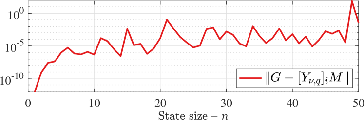
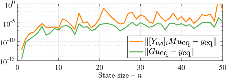
Figure 1: Montecarlo simulations illustrating precision of data-driven transfer function computed according to Theorem V.1, for increasing system size $n$. The curves illustrate the average over $100$ experiments, where matrices $A$ and $B$ have been populated with random i.i.d. normal entries and where the modulus of the eigenvalues of $A$ has been chosen in the interval $(0,1)$. All computations have been carried out using the built-in function mldivide in Matlab 2019a. (a) Error between closed-form expression (4) and the characterization in Theorem V.1 . (b) Error in predicting the steady-state output by using (4) and by using Theorem V.1. ${u}_{\textup{eq}}$ is chosen randomly with i.i.d. entries and ${y}_{\textup{eq}}$ is obtained by running (2) to convergence.

V-B Unknown Noise Terms: Inexact Transfer Function

While Theorem V.1 provides a way to compute $G$ from data, it requires full knowledge of the disturbance $w_{[0,T-1]}$, which is impractical when the exogenous disturbance is unknown. To this end, in the following result we characterize the error that originates when applying ((i)) with unknown $w_{[0,T-1]}$.

Proposition V.3

(Error Characterization) Let Assumption 1 hold and let $\nu\in\mathbb{Z}_{>0}$ denote the observability index of (2). Moreover, assume $u_{[0,T-1]}$ and $w_{[0,T-1]}$ are persistently exciting signals of order $n+\nu$, and let $q:=T-\nu+1$. Assume $\hat{M}\in{}^{q\times m\nu}$ is any matrix that satisfies:

$${Y}^{\textup{diff}}_{\nu,q}\hat{M} =0, U_{\nu,q}\hat{M} =\mathds{1}_{\nu}\otimes I_{m},$$ (26)

where ${Y}^{\textup{diff}}_{\nu,q}$ is defined according to (V-A). If $\hat{G}$ is computed as $\hat{G}:=[Y_{\nu,q}]_{i}\hat{M}$, for any $i\in\{1,\dots,\nu\}$, then

$$\hat{G}-G =CA([X_{\nu,q}]_{i}\hat{M}-(I-A)^{\scalebox{0.75}[0.9]{$-$}1}B)$$

$$\quad\quad+(CE+D)[W_{\nu,q}]_{i}\hat{M}+D[{W}^{\textup{diff}}_{\nu,q}]_{i}\hat{M}.$$ (27)

Proof:

Let $M$ be any matrix as in ((i)) and $\hat{M}$ be any matrix as in (26). By noting that $\hat{G}-G=[Y_{\nu,q}]_{i}(\hat{M}-M)$, we will prove this claim by showing that $[Y_{\nu,q}]_{i}(\hat{M}-M)$ equals the right hand side of (V.3). By using $[{Y}^{\textup{diff}}_{\nu,q}]_{i}M=0$, $[{Y}^{\textup{diff}}_{\nu,q}]_{i}\hat{M}=0$, and by recalling that $[{Y}^{\textup{diff}}_{\nu,q}]_{i}=C(A-I)[X_{\nu,q}]_{i}+CB[U_{\nu,q}]_{i}+CE[W_{\nu,q}]_{i}+D[{W}^{\textup{diff}}_{\nu,q}]_{i}$:

$$0 =[{Y}^{\textup{diff}}_{\nu,q}]_{i}(\hat{M}-M)$$ (28)

$$=C(A-I)[X_{\nu,q}]_{i}(\hat{M}-M)+CB[U_{\nu,q}]_{i}(\hat{M}-M)$$

$$\quad\quad+CE[W_{\nu,q}]_{i}(\hat{M}-M)+D[{W}^{\textup{diff}}_{\nu,q}]_{i}(\hat{M}-M),$$

$$=C(A-I)[X_{\nu,q}]_{i}(\hat{M}-M)+CE[W_{\nu,q}]_{i}\hat{M}+D[{W}^{\textup{diff}}_{\nu,q}]_{i}\hat{M},$$

where we used $[U_{\nu,q}]_{i}\hat{M}=[U_{\nu,q}]_{i}M$, $[W_{\nu,q}]_{i}M=0$, and $[{W}^{\textup{diff}}_{\nu,q}]_{i}M=0$. Next, by recalling that $[Y_{\nu,q}]_{i}(\hat{M}-M)=C[X_{\nu,q}]_{i}(\hat{M}-M)+D[W_{\nu,q}]_{i}(\hat{M}-M)$ and by using (28):

$$[Y_{\nu,q}]_{i}(\hat{M}-M) =CA[X_{\nu,q}]_{i}(\hat{M}-M)$$

$$\quad\quad+(CE+D)[W_{\nu,q}]_{i}\hat{M},+D[{W}^{\textup{diff}}_{\nu,q}]_{i}\hat{M}.$$

Finally, by iterating Step 2 in the proof of Theorem V.1, we obtain $[X_{\nu,q}]_{i}M=(I-A)^{\scalebox{0.75}[0.9]{$-$}1}B$, which proves the claim. ∎

By recalling that $(I-A)^{\scalebox{0.75}[0.9]{$-$}1}B=[X_{\nu,q}]_{i}M$, where $M$ is any matrix that satisfies ((i)), (V.3) can equivalently be written as:

$$\hat{G}-G =CA[X_{\nu,q}]_{i}(\hat{M}-M)$$

$$\quad\quad+(CE+D)[W_{\nu,q}]_{i}\hat{M}+D[{W}^{\textup{diff}}_{\nu,q}]_{i}\hat{M}.$$ (29)

Proposition V.3 shows that the absolute error $\hat{G}-G$ is governed by three terms: (i) the difference $[X_{\nu,q}]_{i}\hat{M}-(I-A)^{\scalebox{0.75}[0.9]{$-$}1}B$, which describes the error between an inexact equilibrium point ${x}_{\textup{inexact}}:=[X_{\nu,q}]_{i}\hat{M}u$, for some $u\in{}^{m}$, obtained by using an inexact matrix $\hat{M}$ and an exact equilibrium point ${x}_{\textup{exact}}:=(I-A)^{\scalebox{0.75}[0.9]{$-$}1}Bu$ obtained by using full knowledge of the system model, (ii) the quantity $[W_{\nu,q}]_{i}\hat{M}$, which can be made equal to zero only when the training data $w_{[0,T-1]}$ is known, and, similarly, (iii) the quantity $[{W}^{\textup{diff}}_{\nu,q}]_{i}\hat{M}$, which can also be made equal to zero only when $w_{[0,T-1]}$ is known. We discuss in the following remark the relationship between Theorem V.1 and Proposition V.3.

Remark 6

(Relationship Between Theorem V.1 and Proposition V.3) We note that if, in addition to (26), $\hat{M}$ satisfies:

$${W}^{\textup{diff}}_{\nu,q}\hat{M}=0,\text{ and }W_{\nu,q}\hat{M}=0,$$

then the following identity holds: $[X_{\nu,q}]_{i}\hat{M}=(I-A)^{\scalebox{0.75}[0.9]{$-$}1}B$, and thus $\hat{G}-G=0$. Hence, in this case, we recover the characterization presented in Theorem V.1. To show that $(I-A)^{\scalebox{0.75}[0.9]{$-$}1}B=[X_{\nu,q}]_{i}\hat{M}$, we recall that $[{Y}^{\textup{diff}}_{\nu,q}]_{i}=C(A-I)[X_{\nu,q}]_{i}+CB[U_{\nu,q}]_{i}+CE[W_{\nu,q}]_{i}+D[{W}^{\textup{diff}}_{\nu,q}]_{i}$ and, by using $[{Y}^{\textup{diff}}_{\nu,q}]_{i}\hat{M}=0$, $[U_{\nu,q}]_{i}\hat{M}=I$, $[W_{\nu,q}]_{i}\hat{M}=0$, and $[{W}^{\textup{diff}}_{\nu,q}]_{i}\hat{M}=0$, we have:

$$0=C(A-I)[X_{\nu,q}]_{i}\hat{M}+CB.$$

Since the system is observable and the above identity holds for all $i\in\{1,\dots,\nu\}$, we obtain that $[X_{\nu,q}]_{i}\hat{M}=(A-I)^{\scalebox{0.75}[0.9]{$-$}1}B$ (see Step 2 in the proof of Theorem V.1), thus proving the equivalence. $\square$

It follows from Remark 6 that, in the special case where the training data is noiseless (i.e., $W_{\nu,q}={W}^{\textup{diff}}_{\nu,q}=0$), Proposition V.3 guarantees that $\hat{G}=G$. Finally, we discuss in the following corollary the special case where matrix $C$ is full column-rank.

Corollary V.4

(Error Characterization for Full Column-Rank $C$) Let Assumption 1 be satisfied and let $\hat{G}$ be as in (V.3). If the Observability is $\nu=1$, then

$$\hat{G}-G =\Big{(}C(I-A)^{\scalebox{0.75}[0.9]{$-$}1}E[W_{\nu,q}]_{i}+D[W_{\nu,q}]_{i}$$ (30)

$$\quad\quad\quad\quad\quad\quad+C(I-A)^{\scalebox{0.75}[0.9]{$-$}1}C^{\dagger}D[{W}^{\textup{diff}}_{\nu,q}]_{i}\Big{)}\hat{M}.$$

Proof:

When $\nu=1$, then $C$ is of full column-rank, and in this case (28) implies:

$$[X_{\nu,q}]_{i}(\hat{M}-M) =(A-I)^{\scalebox{0.75}[0.9]{$-$}1}E[W_{\nu,q}]_{i}\hat{M}$$

$$\quad\quad+(A-I)^{\scalebox{0.75}[0.9]{$-$}1}C^{\dagger}D[{W}^{\textup{diff}}_{\nu,q}]_{i}\hat{M}.$$

The claim follows by recalling that $[Y_{\nu,q}]_{i}(\hat{M}-M)=C[X_{\nu,q}]_{i}(\hat{M}-M)+D[W_{\nu,q}]_{i}(\hat{M}-M)$. ∎

We conclude this section by discussing the particular case in which $\hat{M}$ is chosen as the (unique) minimum-norm solution of the set of equations (26).

Example 1

(Optimal Selection of Training Data) Let $\hat{M}^{*}$ be the minimum-norm solution of (26):

$$\hat{M}^{*}:=\arg\min_{\hat{M}\in{}^{q\times m\nu}}~{}~{}~{} \|\hat{M}\|_{F}$$

s.t. $${Y}^{\textup{diff}}_{\nu,q}\hat{M}=0,~{}~{}U_{\nu,q}\hat{M}=\mathds{1}_{\nu}\otimes I_{m},$$

where we recall that $\|\hat{M}\|_{F}$ denotes the Frobenius norm of $\hat{M}$. Then, $\hat{M}^{*}$ can be written as:

$$\hat{M}^{*}=\begin{bmatrix}{Y}^{\textup{diff}}_{\nu,q}\\ U_{\nu,q}\end{bmatrix}^{\dagger}\begin{bmatrix}0\\ I\end{bmatrix}:=\begin{bmatrix}Y^{+}~{}U^{+}\end{bmatrix}\begin{bmatrix}0\\ \mathds{1}_{\nu}\otimes I_{m}\end{bmatrix}=U^{+}(\mathds{1}_{\nu}\otimes I_{m}),$$

where $Y^{+}\in{}^{q\times p\nu}$ and $U^{+}\in{}^{q\times m\nu}$ are matrices that satisfy the identities: ${Y}^{\textup{diff}}_{\nu,q}Y^{+}=I$, $U_{\nu,q}Y^{+}=0$, ${Y}^{\textup{diff}}_{\nu,q}U^{+}=0$, and $U_{\nu,q}U^{+}=I$. The above equation implies $[W_{\nu,q}]_{i}\hat{M}=[W_{\nu,q}]_{i}U^{+}$ and $[{W}^{\textup{diff}}_{\nu,q}]_{i}\hat{M}=[W_{\nu,q}]_{i}U^{+}$.

By combining these relationships with (30), we have:

$$\|\hat{G}-G\| \leq\|C(I-A)^{\scalebox{0.75}[0.9]{$-$}1}E+D\|\|[W_{\nu,q}]_{i}\hat{M}\|$$

$$\quad\quad\quad\quad\quad\quad+\|C(I-A)^{\scalebox{0.75}[0.9]{$-$}1}C^{\dagger}D\|\|[{W}^{\textup{diff}}_{\nu,q}]_{i}\hat{M}\|$$

$$\leq\|C(I-A)^{\scalebox{0.75}[0.9]{$-$}1}E+D\|\|[W_{\nu,q}]_{i}U^{+}\|$$

$$\quad\quad\quad\quad\quad\quad+\|C(I-A)^{\scalebox{0.75}[0.9]{$-$}1}C^{\dagger}D\|\|[{W}^{\textup{diff}}_{\nu,q}]_{i}U^{+}\|.$$

Since $U^{+}$ is a right-inverse of $U_{\nu,q}$, the above bound suggests that $G-\hat{G}=0$ can be obtained when the signal $u_{[0,T-1]}$ is chosen so that the rows of $W_{\nu,q}$ and of ${W}^{\textup{diff}}_{1,q}$ are orthogonal to the columns of the matrix $U^{+}$. $\blacksquare$

VI Tracking Performance in the Presence of Time-Varying Disturbances

Having solved challenges (Ch1)-(Ch3), we are now ready to characterize the transient performance of the controller (IV-B). To this aim, we let

$$e_{k} :=\nabla_{u}\phi(u_{k},y_{k})+\hat{G}^{\mathsf{T}}\nabla_{y}\phi(u_{k},y_{k})$$

$$\quad\quad\quad\quad-\mathbb{E}_{y_{k}}[\nabla_{u}\phi(u_{k},y_{k})+\hat{G}^{\mathsf{T}}\nabla_{y}\phi(u_{k},y_{k})],$$ (31)

denote the gradient error that originates from using a single-point gradient approximation based on the measurement of the output of the system.

Remark 7

(Common Assumptions That Guarantee Bounded Gradient Error) In what follows, we make the implicit assumption that the gradient error $\mathbb{E}[\|e_{k}\|]$ is bounded. Such assumption is commonly adopted in the literature (see e.g. [42] for a thorough discussion). Commonly-adopted assumptions that guarantee boundedness of the gradient error include uniform boundedness assumptions of the form:

$$\mathbb{E}[\|e_{k}\|]<\sigma,\text{ for all }k\in\mathbb{Z}_{\geq 0},$$

for some $\sigma\in{}_{>0}$, or bounded variance assumptions of the form:

$$\mathbb{E}[\|e_{k}\|^{2}]\leq\|\mathbb{E}_{y_{k}}[\nabla_{u}\phi(u_{k},y_{k})+\hat{G}^{\mathsf{T}}\nabla_{y}\phi(u_{k},y_{k})]\|^{2}+\bar{\sigma}^{2}.$$

for some $\bar{\sigma}\in\mathbb{R}_{\geq 0}$. We also notice that – except for the use of the 1-norm as opposed to the 2-norm – due to unbiasedness, uniform boundedness and bounded variance assumptions are equivalent. $\square$

Theorem VI.1

(Tracking of Time-Varying Stable Optimizer) Let Assumption 2 be satisfied, and let $\xi_{k}:=(x_{k},u_{k})$ and ${\xi}^{\textup{so}}_{k}:=({x}^{\textup{so}}_{k},{u}^{\textup{so}}_{k})$, where ${u}^{\textup{so}}_{k}$ and ${x}^{\textup{so}}_{k}$ are as in Definition IV.1. Then, for any $k\in\mathbb{Z}_{\geq 0}$, the solutions of (IV-B) satisfy:

$$\mathbb{E}[\|\xi_{k+1}-{\xi}^{\textup{so}}_{k+1}\|]\leq\beta_{1}\mathbb{E}\left[\|u_{k}-{u}^{\textup{so}}_{k}\|\right]+\beta_{2}\mathbb{E}\left[\|x_{k}-{x}^{\textup{so}}_{k}\|\right]$$

$$\quad+\gamma_{1}\mathbb{E}[\|e_{k}\|]+\gamma_{2}\|{u}^{\textup{so}}_{k+1}-{u}^{\textup{so}}_{k}\|+\gamma_{3}\mathbb{E}[\sup_{t\in\mathbb{Z}_{\geq 0}}\|{x}^{\textup{so}}_{k+1}-{x}^{\textup{so}}_{k}\|],$$ (32)

where $e_{k}$ defined in (VI) and, for any $\kappa\in(0,1)$,

$$\beta_{1} =\sqrt{1-\eta\mu}+\eta\hat{\ell}^{\nabla}\|G-\hat{G}\|,\quad\hat{\ell}^{\nabla}:=\ell_{u}^{\nabla}+\|\hat{G}\|\ell_{y}^{\nabla},$$

$$\beta_{2} =\sqrt{\frac{\bar{\lambda}(P)}{\underline{\lambda}(P)}\left(1-(1\!-\!\kappa)\frac{\underline{\lambda}(Q)}{\bar{\lambda}(P)}\right)}+\eta\hat{\ell}^{\nabla}\|C\|,$$

$$\gamma_{1} =\eta,\quad\gamma_{2}=1,\quad\gamma_{3}=\max\{\sqrt{\frac{2\bar{\lambda}(P)}{\kappa\underline{\lambda}(Q)}},\frac{4\|A^{\mathsf{T}}P\|}{\kappa\underline{\lambda}(Q)}\}.$$

Moreover, if $\beta_{1}<1$ and $\beta_{2}<1$, then ${u}^{\textup{so}}_{k}$ exists and is unique.

Proof:

The proof is organized into four main steps.

(1 – Change of Variables and Contraction Bound) Define the change of variables $\tilde{x}_{k}:=x_{k}-{x}^{\textup{so}}_{k}=x_{k}-(I-A)^{\scalebox{0.75}[0.9]{$-$}1}B{u}^{\textup{so}}_{k}-(I-A)^{\scalebox{0.75}[0.9]{$-$}1}Ew_{k}$. Accordingly, (IV-B) read as:

$$\tilde{x}_{k+1} =A\tilde{x}_{k}+(x_{k}^{*}-x_{k+1}^{*}),$$

$$u_{k+1} =u_{k}-\eta(\nabla_{u}\phi(u_{k},C\tilde{x}_{k}+\hat{G}u_{k}+\bar{z})$$

$$\quad\quad\quad\quad\quad\quad+\hat{G}^{\mathsf{T}}\nabla_{u}\phi(u_{k},C\tilde{x}_{k}+\hat{G}u_{k}+\bar{z})).$$

Next, we introduce the following compact notation to denote the algorithmic updates (IV-B) for all $\theta\in{}^{m}$, $u\in{}^{m}$, $x\in{}^{n}$:

$$F_{\theta}(u,x) :=\underset{\mathcal{Z}(\theta)}{\mathbb{E}}[\nabla_{u}\phi(u,Cx+\hat{G}u+z)$$ (33)

$$\quad\quad\quad\quad\quad\quad\quad+\hat{G}^{\mathsf{T}}\nabla_{y}\phi(u,Cx+\hat{G}u+z)],$$

$$\hat{F}(u,x) :=\nabla_{u}\phi(u,Cx+\hat{G}u+z)$$

$$\quad\quad\quad\quad\quad\quad\quad+\hat{G}^{\mathsf{T}}\nabla_{y}\phi(u,Cx+\hat{G}u+z),$$

$$\mathcal{C}_{\theta}(u,x) :=u-\eta F_{\theta}(u,x),\quad\mathcal{\hat{C}}(u,x):=u-\eta\hat{F}(u,x).$$

Accordingly, the left hand side of (VI.1) satisfies:

$$\mathbb{E}[\|\xi_{k+1}-{\xi}^{\textup{so}}_{k+1}\|]\leq\mathbb{E}[\|u_{k+1}-{u}^{\textup{so}}_{k+1}\|]+\mathbb{E}[\|\tilde{x}_{k+1}\|]$$ (34)

$$\quad\quad\quad\leq\mathbb{E}[\|u_{k+1}-{u}^{\textup{so}}_{k}\|]+\|{u}^{\textup{so}}_{k+1}-{u}^{\textup{so}}_{k}\|+\mathbb{E}[\|\tilde{x}_{k+1}\|],$$

where we used $\mathbb{E}[\|{u}^{\textup{so}}_{k+1}-{u}^{\textup{so}}_{k}\|]=\|{u}^{\textup{so}}_{k+1}-{u}^{\textup{so}}_{k}\|$ since stable optimizers are deterministic quantities. Moreover, notice that:

$$\mathbb{E}[\|u_{k+1}-{u}^{\textup{so}}_{k}\|] =\mathbb{E}[\|\mathcal{\hat{C}}(u_{k},\tilde{x})-\mathcal{C}_{{u}^{\textup{so}}_{k}}({u}^{\textup{so}}_{k},0)\|]$$

$$\leq\mathbb{E}[\|e_{k}\|]+\|\mathcal{C}_{u_{k}}(u_{k},\tilde{x})-\mathcal{C}_{{u}^{\textup{so}}_{k}}(u_{k},\tilde{x}_{k})\|$$

$$\quad+\|\mathcal{C}_{{u}^{\textup{so}}_{k}}(u_{k},\tilde{x}_{k})-\mathcal{C}_{{u}^{\textup{so}}_{k}}(u_{k},0)\|$$

$$\quad+\|\mathcal{C}_{{u}^{\textup{so}}_{k}}(u_{k},0)-\mathcal{C}_{{u}^{\textup{so}}_{k}}({u}^{\textup{so}}_{k},0)\|.$$ (35)

where we used $\mathcal{\hat{C}}(u_{k},\tilde{x})-\mathcal{C}_{u_{k}}(u_{k},\tilde{x})=e_{k}$ and we remark that the last three terms are deterministic quantities. Linear convergence of (IV-B) is a direct consequence of three independent properties, namely contraction at the equilibrium, calmness to distributional shifts, and ease with respect to system dynamics, which we prove next.

(2 – Calmness With Respect to Distributional Shifts) We will show: $\|\mathcal{C}_{u_{k}}(u_{k},\tilde{x}_{k})-\mathcal{C}_{{u}^{\textup{so}}_{k}}(u_{k},\tilde{x}_{k})\|\leq\eta\hat{\ell}^{\nabla}\|G-\hat{G}\|\|u_{k}-{u}^{\textup{so}}_{k}\|$. Indeed, the following estimate holds:

$$\|\mathcal{C}_{u_{k}}(u_{k},\tilde{x}_{k})-\mathcal{C}_{{u}^{\textup{so}}_{k}}(u_{k},\tilde{x}_{k})\| \leq\eta\hat{\ell}^{\nabla}W_{1}(\mathcal{Z}(u_{k}),\mathcal{Z}({u}^{\textup{so}}_{k}))$$

$$\leq\eta\hat{\ell}^{\nabla}\|G-\hat{G}\|\|u_{k}-{u}^{\textup{so}}_{k}\|,$$

where the first inequality follows by expanding (33) and by using Lemma II.5, and the second inequality follows from (9).

(3 – Ease With Respect to the System Dynamics) We will show that $\|\mathcal{C}_{{u}^{\textup{so}}_{k}}(u_{k},\tilde{x}_{k})-\mathcal{C}_{\tilde{u}_{k}^{*}}(u_{k},0)\|\leq\eta\hat{\ell}^{\nabla}\|C\|\|\tilde{x}_{k}\|$. By using Assumption 2(b):

$$\|\mathcal{C}_{{u}^{\textup{so}}_{k}}(u_{k},\tilde{x}_{k})-\mathcal{C}_{{u}^{\textup{so}}_{k}}(u_{k},0)\|$$

$$\leq\eta\|\mathbb{E}_{\mathcal{Z}_{k}({u}^{\textup{so}}_{k})}\left[\nabla_{u}\phi(u_{k},C\tilde{x}_{k}\!+\!\hat{G}u_{k}\!+\!z)-\nabla_{u}\phi(u_{k},\hat{G}u_{k}\!+\!z)\right]\|$$

$$~{}+\eta\|\hat{G}^{\mathsf{T}}\!\mathbb{E}_{\mathcal{Z}_{k}({u}^{\textup{so}}_{k})}\left[\nabla_{y}\phi(u_{k},C\tilde{x}_{k}\!+\!\hat{G}u_{k}\!+\!z)-\nabla_{y}\phi(u_{k},\hat{G}u_{k}\!+\!z)\right]\|$$

$$\leq\eta\hat{\ell}^{\nabla}\|C\|\|\tilde{x}_{k}\|,$$

which proves the claimed estimate.

(4 – Contraction at the Equilibrium) We will show that $\|\mathcal{C}_{{u}^{\textup{so}}_{k}}(u_{k},0)-\mathcal{C}_{{u}^{\textup{so}}_{k}}({u}^{\textup{so}}_{k},0)\|\leq\sqrt{1-\eta\mu}\|u_{k}-{u}^{\textup{so}}_{k}\|$. This fact follows directly from [37, Thm 3.12], and we provide a short proof for completeness. By substituting (33):

$$\|\mathcal{C}_{{u_{k}}^{\textup{so}}_{k}}(u,0)-\mathcal{C}_{{u}^{\textup{so}}_{k}}({u}^{\textup{so}}_{k},0)\|^{2}=\|u-\eta F_{{u}^{\textup{so}}_{k}}(u_{k},0)-{u}^{\textup{so}}_{k}\|^{2}$$

$$~{}=\|u_{k}\!-\!{u}^{\textup{so}}_{k}\|^{2}-2\eta F_{{u}^{\textup{so}}_{k}}(u_{k},0)^{\mathsf{T}}(u_{k}\!-\!{u}^{\textup{so}}_{k})+\eta^{2}\|F_{{u}^{\textup{so}}_{k}}(u_{k},0)\|^{2}$$

$$~{}\leq(1-\eta\mu)\|u_{k}\!-\!{u}^{\textup{so}}_{k}\|^{2}-2\eta\Big{(}\mathbb{E}_{\mathcal{Z}({u}^{\textup{so}}_{k})}\left[\phi(u_{k},C\tilde{x}_{k}+\hat{G}u_{k}+z)\right]$$

$$\quad\quad+\mathbb{E}_{\mathcal{Z}({u}^{\textup{so}}_{k})}\left[\phi({u}^{\textup{so}}_{k},C\tilde{x}_{k}+\hat{G}{u}^{\textup{so}}_{k}+z)\right]\Big{)}+\eta^{2}\|F_{{u}^{\textup{so}}_{k}}(u_{k},0)\|^{2}$$

$$~{}\leq(1-\eta\mu)\|u_{k}-{u}^{\textup{so}}_{k}\|^{2}+\alpha\Big{(}\mathbb{E}_{\mathcal{Z}({u}^{\textup{so}}_{k})}\left[\phi(u_{k},C\tilde{x}_{k}+\hat{G}u_{k}+z)\right]$$

$$\quad\quad-\mathbb{E}_{\mathcal{Z}({u}^{\textup{so}}_{k})}\left[\phi({u}^{\textup{so}}_{k},C\tilde{x}_{k}+\hat{G}{u}^{\textup{so}}_{k}+z)\right]\Big{)}$$

$$\quad\leq(1-\eta\mu)\|u_{k}-{u}^{\textup{so}}_{k}\|^{2},$$

where $\alpha=2(\eta^{2}\hat{\ell}^{\nabla}-\eta)$. Above, the first inequality follows from $\phi(u_{k},z_{k})-\phi(u_{k},{z}^{\textup{so}}_{k})\geq\nabla\phi(u_{k},{z}^{\textup{so}}_{k})^{\mathsf{T}}(u_{k}-{u}^{\textup{so}}_{k})+\frac{\mu}{2}\|u_{k}-{u}^{\textup{so}}_{k}\|^{2}$ (see Assumption 2(c)), the second inequality follows from $\|F_{{u}^{\textup{so}}_{k}}(u_{k},0)\|^{2}\leq 2\hat{\ell}^{\nabla}(\phi(u_{k},z_{k})-\phi(u_{k},{z}^{\textup{so}}_{k}))$ (see Assumption  2(b)), and the last inequality holds because ${u}^{\textup{so}}_{k}$ is a stable optimizer (see (7)).

(5 – Contraction of the Dynamical System) We will prove the following estimate:

$$\mathbb{E}[\|\tilde{x}_{k+1}\|]\leq\sqrt{\frac{\bar{\lambda}(P)}{\underline{\lambda}(P)}\left(1-\frac{\underline{\lambda}(Q)}{4\bar{\lambda}(P)}\right)}\mathbb{E}[\|\tilde{x}_{k}\|]$$ (36)

$$\quad\quad+\max\{\sqrt{\frac{4\bar{\lambda}(P)}{\underline{\lambda}(Q)}},\frac{4\|A^{\mathsf{T}}P\|}{\underline{\lambda}(Q)}\}\mathbb{E}[\sup_{t\in\mathbb{Z}_{\geq 0}}\|{x}^{\textup{so}}_{k+1}-{x}^{\textup{so}}_{k}\|].$$

In what follows, we fix the realization of the disturbance $w_{k}$ and (with a slight abuse of notation) we denote by $\tilde{x}_{k}$ the corresponding (deterministic) state of (2) and by ${x}^{\textup{so}}_{k}$ the associated (deterministic) stable optimizer. Let $V(x):=x^{\mathsf{T}}Px$ and define the set:

$$\Omega :=\{x\in{}^{n}:V(x)\leq\frac{4\bar{\lambda}(P)\|A^{\mathsf{T}}P\|}{\underline{\lambda}(Q)}\sup_{t\in\mathbb{Z}_{\geq 0}}\|{x}^{\textup{so}}_{t+1}-{x}^{\textup{so}}_{t}\|$$

$$\quad\quad\quad\quad\text{ and }V(x)\leq\bar{\lambda}(P)\sqrt{\frac{4\bar{\lambda}(P)}{\underline{\lambda}(Q)}}\sup_{t\in\mathbb{Z}_{\geq 0}}\|{x}^{\textup{so}}_{t+1}-{x}^{\textup{so}}_{t}\|\}.$$

We distinguish among two cases.

(5 – Case 1) Suppose $\tilde{x}_{k}\not\in\Omega$. In this case, we have:

$$V(\tilde{x}_{k+1})-V(\tilde{x}_{k}) \leq-\underline{\lambda}(Q)\|\tilde{x}_{k}\|^{2}+\bar{\lambda}(P)\|{x}^{\textup{so}}_{k+1}-{x}^{\textup{so}}_{k}\|^{2}$$

$$\quad\quad+2\|A^{\mathsf{T}}P\|\|{x}^{\textup{so}}_{k+1}-{x}^{\textup{so}}_{k}\|\|\tilde{x}_{k}\|$$

$$\leq-\frac{1}{4}\frac{\underline{\lambda}(Q)}{\bar{\lambda}(P)}V(\tilde{x}_{k}),$$ (37)

where the last inequality follows since $\tilde{x}_{k}\not\in\Omega$ and by using $V(\tilde{x}_{k})\leq\bar{\lambda}(P)\|\tilde{x}_{k}\|^{2}$. By using $\underline{\lambda}(P)\|\tilde{x}_{k}\|^{2}\leq V(\tilde{x}_{k})\leq\bar{\lambda}(P)\|\tilde{x}_{k}\|^{2}$, (VI) implies the following bound for the state:

$$\|\tilde{x}_{k+1}\|^{2}\leq\frac{\bar{\lambda}(P)}{\underline{\lambda}(P)}\left(1-\frac{\underline{\lambda}(Q)}{4\bar{\lambda}(P)}\right)\|\tilde{x}_{k}\|^{2}.$$ (38)

(5 – Case 2) Suppose $\tilde{x}_{k}\in\Omega$. In this case, we will show that $\Omega$ is forward-invariant, i.e., $\tilde{x}_{k+1}\in\Omega$. By contradiction, let $\epsilon>0$ and let $k_{1}$ be the first instant such that one of the following conditions is satisfied:

$$V(\tilde{x}_{k_{1}}) >\bar{\lambda}(P)\frac{4\|A^{\mathsf{T}}P\|}{\underline{\lambda}(Q)}\sup_{t\in\mathbb{Z}_{\geq 0}}\|{x}^{\textup{so}}_{t+1}-{x}^{\textup{so}}_{t}\|+\epsilon,\text{ or}$$

$$V(\tilde{x}_{k_{1}}) >\bar{\lambda}(P)\sqrt{\frac{4\bar{\lambda}(P)}{\underline{\lambda}(Q)}}\sup_{t\in\mathbb{Z}_{\geq 0}}\|{x}^{\textup{so}}_{t+1}-{x}^{\textup{so}}_{t}\|+\epsilon,$$ (39)

It follows by iterating (VI) that $V(\tilde{x}_{k})$ is strictly decreasing in a neighborhood of $k_{1}$. Accordingly, there must exists $0\leq k_{0}<k_{1}$ such that $V(\tilde{x}_{k_{0}})>V(\tilde{x}_{k_{1}})$. But this contradicts the assumption that $k_{1}$ is the first instant that satisfies (VI). So $\Omega$ must be forward invariant. By recalling the definition of $\Omega$, when $\tilde{x}_{k}\in\Omega$:

$$\|\tilde{x}_{k+1}\|\leq\max\{\sqrt{\frac{4\bar{\lambda}(P)}{\underline{\lambda}(Q)}},\frac{4\|A^{\mathsf{T}}P\|}{\underline{\lambda}(Q)}\}\sup_{t\in\mathbb{Z}_{\geq 0}}\|{x}^{\textup{so}}_{k+1}-{x}^{\textup{so}}_{k}\|.$$ (40)

Finally, the estimate (36) follows by combining (38) and (40) and by taking the expectation on both sides.

To conclude, (VI.1) follows by substituting the estimates derived in the above five steps into (34)–(VI). Notice that, existence and uniqueness of ${u}^{\textup{so}}_{k}$ follows from contractivity and by application of the Banach fixed-point theorem. ∎

Remark 8

(Choices of $\eta$ that guarantee $\beta_{1}<1$) To guarantee $\beta_{1}<1$, the following conditions must hold simultaneously:

$$\|G-\hat{G}\|<\frac{\mu}{\hat{\ell}^{\nabla}},\quad\text{ and }\quad\frac{2\|G-\hat{G}\|-\mu}{\|G-\hat{G}\|^{2}}<\eta\leq\frac{1}{\mu}.$$ (41)

Note that for any $\mu\in{}_{>0}$ and $\hat{G}\in{}^{p\times m}$, there exists a nonempty set of choices of $\eta$ that satisfy the second condition in (41). To see this, notice that $\frac{2\|G-\hat{G}\|-\mu}{\|G-\hat{G}\|^{2}}\leq\frac{1}{\mu}$ is equivalent to $(\|G-\hat{G}\|-\mu)^{2}\geq 0$, which is satisfied for any $\mu\in{}_{>0}$ and $\hat{G}\in{}^{p\times m}$. While there always exists a choice of $\eta$ that guarantees the second condition, the first inequality in (41) outlines a feasibility condition. Namely, when the absolute error $\|G-\hat{G}\|$ is larger than the constant $\mu/\hat{\ell}^{\nabla}$, then the controller (IV-B) cannot guarantee contractivity.

To derive (41), notice that $\sqrt{1-\eta\mu}$ admits a real-valued solution if an only if $\eta\leq 1/\mu$. Moreover, the equation $\sqrt{1-\eta\mu}+\eta\hat{\ell}^{\nabla}\|G-\hat{G}\|=1$ yields the solution $\eta=\eta_{1}:=0$ and $\eta=\eta_{2}:=(2\|G-\hat{G}\|-\mu)/\|G-\hat{G}\|^{2}$, where $\eta_{2}$ is real only if $\hat{\ell}^{\nabla}\|G-\hat{G}\|\leq\mu$. Accordingly, $\beta_{1}<1$ when $\eta<\eta_{1}$ or $\eta>\eta_{2}$ (see Fig. 2), which yields (41). $\square$

Remark 9

(Choices of $\eta$ that guarantee $\beta_{2}<1$) To guarantee $\beta_{2}<1$ the controller $\eta$ must be chosen as:

$$\eta<\frac{1}{\hat{\ell}^{\nabla}\|C\|}\left(1-\sqrt{\frac{\bar{\lambda}(P)}{\underline{\lambda}(P)}\left(1-(1\!-\!\kappa)\frac{\underline{\lambda}(Q)}{\bar{\lambda}(P)}\right)}~{}\right).$$

Notice that the quantity $\frac{\bar{\lambda}(P)}{\underline{\lambda}(P)}\left(1-(1\!-\!\kappa)\frac{\underline{\lambda}(Q)}{\bar{\lambda}(P)}\right)$ is always non-negative since $\underline{\lambda}(Q)/\bar{\lambda}(P)<1$ and it strictly smaller that $1$ if the open-loop dynamics (2) are contractive. $\square$

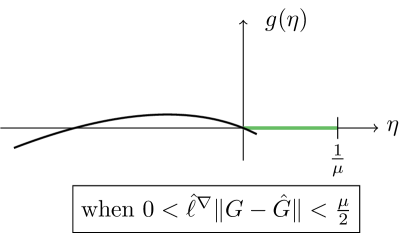
Figure 2: Roots of $g(\eta)=\sqrt{1-\eta\mu}+\eta\hat{\ell}^{\nabla}\|G-\hat{G}\|-1$. The green segment illustrates the set of choices of $\eta$ that guarantee $\beta_{1}<1$.

Theorem VI.1 provides a sufficient condition to guarantee that the controlled dynamics (IV-B) converge to a stable optimizer $({x}^{\textup{so}}_{k},{u}^{\textup{so}}_{k})$ (up to an asymptotic error that depends on the time-variability of the optimizer and on the sampling error). This result, combined with Proposition IV.2, allows us to conclude convergence to a small neighborhood of the desired optimizer $(x_{k}^{*},u_{k}^{*})$.

According to Theorem VI.1, the rate of contraction of (IV-B) depends on various parameters of the optimization problem as well as of the dynamical system: it increases with the square root of $\eta$, $\mu$, and of the ratio $\underline{\lambda}(Q)/\bar{\lambda}(P)$ (that characterizes the rate of convergence of the open-loop plant (2)), and it is inversely proportional to $\eta$, $\hat{\ell}^{\nabla}$, $\|G-\hat{G}\|$, and $\|C\|$. Moreover, there are three error terms that affect the bound: the error between the sample-based and true gradient $\|e_{k}\|$, the shift in the stable input optimizer $\|{u}^{\textup{so}}_{k+1}-{u}^{\textup{so}}_{k}\|$, and the worse-case shift in the stable state optimizer $\sup_{t\in\mathbb{Z}_{\geq 0}}\|{x}^{\textup{so}}_{t+1}-{x}^{\textup{so}}_{t}\|$.

Some important comments on the choice of $\eta$ are in order. First, as discussed in Remark 8, when the distributional shifts originated by the controller update are small (i.e., $\hat{\ell}^{\nabla}\|G-\hat{G}\|<\mu/2$), then a sufficiently-slow controller (i.e, $\eta\leq 1/\mu$) guarantees contraction in (VI.1). On the other hand, when the distributional shifts originated by the controller updates are large (i.e., $\hat{\ell}^{\nabla}\|G-\hat{G}\|>\mu/2$), then there is a lower bound on the required controller gain to guarantee contractivity (namely, $\eta>(2\|G-\hat{G}\|-\mu)/\|G-\hat{G}\|^{2}$). This fact can be interpreted by noting that a sufficiently-large controller gain guarantees that deviations introduced by shifts in the distribution (i.e. the term $\eta\hat{\ell}^{\nabla}\|G-\hat{G}\|$) are dominated by the the algorithm contractivity towards the optimizer (i.e., the term $\sqrt{1-\eta\mu}$). See the proof of Theorem VI.1, steps 2 and 4. We note that this fact is in contrast with standard conditions for convergence of gradient-descent (see e.g. [37]), where arbitrarily-small choices of the controller gain always guarantee contractivity of the updates.

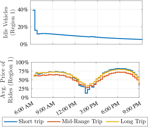
Figure 3: (a) Case study: Manhattan, NY, partitioned into $18$ regions of ride requests. (b) Number of idle vehicles and cost of trips for region 1. Short trip refers to trips from $1$ to $4$, mid range trip refers from $1$ to $10$, long trip refers from $1$ to $16$. See caption of Figure 5 for detailed experiment description.

VII Application to Ride-Service Scheduling

We illustrate here the versatility and performance of the proposed controller synthesis approach in an application scenario. A ride service provider (RSP), such as Uber, Lyft, or DiDi, seeks to maximize its profit by dispatching the vehicles in its fleet to serve ride requests from its customers. We model the area of interest using a graph $\mathcal{G}=(\mathcal{V},\mathcal{E})$, where each node in $\mathcal{V}$ represents a region (e.g., a block or a district of a city) and an edge $(i,j)\in\mathcal{E}$ allows rides from node $i$ to node $j$. As a case study, we consider Manhattan, NY, and, similarly to [43], we divide the area into $n=18$ region as in Figure 3(a). We assume that time is slotted and each slot has duration $\Delta=5$ min. We let $\delta^{ij}_{k}\in\mathbb{R}_{\geq 0}$ be the demand of rides from region $i\in\mathcal{V}$ to region $j\in\mathcal{V}$ at time $k\in\mathbb{Z}_{\geq 0}$. We denote by $p_{ij}^{k}$ the price of rides, decided by the RSP, from region $i$ to region $j$ at time $k$. We account for elasticity of the demand, whereby customers can decide to accept or decline rides after observing the price set by the RSP, and leave the system when prices are higher that the their maximum willingness to pay. We model the elasticity of the demand as follows:

$$d^{ij}_{k}=\delta^{ij}_{k}\Big{(}1-\theta^{ij}\frac{p^{ij}_{k}}{{p}_{\textup{max}}^{ij}}\Big{)}.$$ (42)

Here, $d^{ij}_{k}$ denotes the accepted demand (after customers have observed the prices set by the RSP) of rides from region $i$ to $j$ at time $k$, $\theta^{ij}\in[0,1]$ is a parameter that characterizes the steepness of elasticity, and ${p}^{\textup{max}}_{ij}\in{}_{>0}$ is an upper limit on prices from $i$ to $j$.

We let $x^{i}_{k}\in\mathbb{R}_{\geq 0}$ denote the idle-vehicle occupancy (i.e., the number of unoccupied vehicles, normalized by the fleet size) of fleet vehicles in region $i$ at time $k$. We assume that drivers of unoccupied vehicles naturally rebalance the fleet, namely, they travel from regions with a high occupancy of (fleet) vehicles to regions with a lower occupancy in order to maximize their profit. We denote by $a_{ij}\in\mathbb{R}_{\geq 0}$ the fraction of unoccupied vehicles that travel from $i$ to $j$ at every time step. Travel times are non-negligible and can vary over time: we model them by using Boolean variables:

$$\sigma^{ij,\tau}_{k}=\begin{cases}1,&\text{if travel time from $i$ to $j$ at time $k$ is $\tau$ slots,}\\ 0,&\text{otherwise},\end{cases}$$

defined for all $i,j\in\mathcal{V}$ and $k,\tau\in\mathbb{Z}_{\geq 0}$. In what follows, we assume that $\sigma^{ij,0}_{k}=0$ for all $i,j\in\mathcal{V},k\in\mathbb{Z}_{\geq 0}$, so vehicles take at least one time slot to travel between any pair of nodes; moreover, we let $\sigma^{ij,\tau}_{k}=0$ for all $\tau>T\in\mathbb{Z}_{\geq 0}$, so that $T$ is the maximum travel time in the network. Accordingly, the occupancy of idle vehicles in each region $i$ satisfies the following conservation law:

$$x_{k+1}^{i} =x_{k}^{i}-\sum_{j\in\mathcal{V}}a_{ij}x_{k}^{i}+\sum_{j\in\mathcal{V}}a_{ji}x_{k}^{j}$$ (43)

$$\quad\quad\quad\quad\quad-\sum_{j\in\mathcal{V}}d^{ij}_{k}+\underbrace{\sum_{j\in\mathcal{V}}\sum_{\tau=k-T}^{k-1}\sigma^{ji,k-\tau}_{\tau}d^{ji}_{\tau}+e_{k}^{i}}_{:=w^{i}_{k}},$$

In (43), the quantity $-\sum_{j\in\mathcal{V}}a_{ij}x_{k}^{i}$ accounts for the vehicles that leave the region due to fleet rebalancing, while $\sum_{j\in\mathcal{V}}a_{ji}x_{k}^{j}$ models rebalancing vehicles arriving at $i$. The quantity $-\sum_{j\in\mathcal{V}}d^{ij}_{k}$ models all customer-occupied vehicles departing $i$ at time $k$, while $\sum_{\tau=0}^{k}\sigma^{ji,k-\tau}_{\tau}d^{ji}_{\tau}$ accounts for occupied vehicles arriving to $i$ at time $k$. Finally, we use the term $e_{k}^{i}$ to account for all the unmodeled disturbances affecting the dynamics, including inaccuracies in the rebalancing coefficients $a_{ij}$ and vehicles leaving or entering the system (e.g., drivers that stop or start driving). Further, we assume that the travel times between regions (i.e., the scalars $\sigma^{ij,\tau}_{k}$) are unknown or difficult to estimate, and we incorporate all unknown terms in the exogenous signal $w_{k}^{i}$.

Because (43) describes a mass conservation law, the dynamics (43) define a compartmental model that is marginally stable [44]. For this reason, we define the state differences $\tilde{x}_{k}^{i}:=x_{k}^{i}-x_{k}^{i+1}$ for all $k\in\mathbb{Z}_{\geq 0}$, $i\in\mathcal{V}$. In these new variables, (43) define a $(n-1)$-dimensional system that is asymptotically stable and thus satisfies Assumption 1.

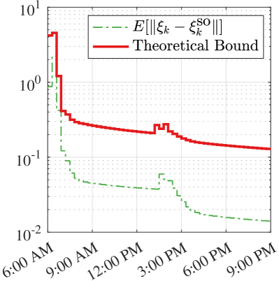
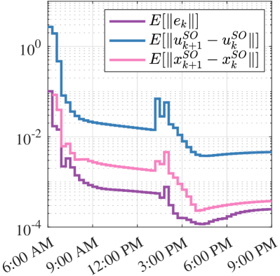
Figure 4: (a) Numerical error and error bound from Theorem VI.1 and (b) terms characterizing the error bound. Curves illustrate the average over $100$ realizations of the noise terms. Fluctuation at around 1:00PM is caused by a drop in ride demands (see Figure 5 (top panel)).

We formulate the RSP’s objectives of selecting the price of rides in order to maximize its profit as the following optimization problem to be solved at every $k$:

$$\max_{p,x,d}~{}~{} \sum_{i\in\mathcal{V}}\sum_{j\in\mathcal{V}}p^{ij}d^{ij}-c^{ij}d^{ij}-\varrho\|x\|^{2},$$

s.t. $$0=-\sum_{j\in\mathcal{V}}a_{ij}x^{i}+\sum_{j\in\mathcal{V}}a_{ji}x^{j}-\sum_{j\in\mathcal{V}}d^{ij}+w_{k}^{i},$$

$$d^{ij}=\delta^{ij}_{k}\left(1-\theta^{ij}p^{ij}/{p}_{\textup{max}}^{ij}\right),$$

$$d^{ij}\geq 0,\;x^{i}\geq 0,\quad\forall i,j,\in\mathcal{V},$$ (44)

where $p,x,d$ denote the vectors obtained by stacking $p^{ij}$, $x^{i}$, and $d^{ij}$, for all $i,j\in\mathcal{V}$, respectively, $p^{ij}d^{ij}$ models the RSP earnings from serving the demand $d^{ij}$, the quantity $c^{ij}d^{ij}$, $c^{ij}\in{}_{>0}$, models the cost of routing vehicles from $i$ to $j$, and the term $\varrho\|x\|$, $\varrho\in{}_{>0}$, describes the RSP’s objective of maximizing the fleet utilization.

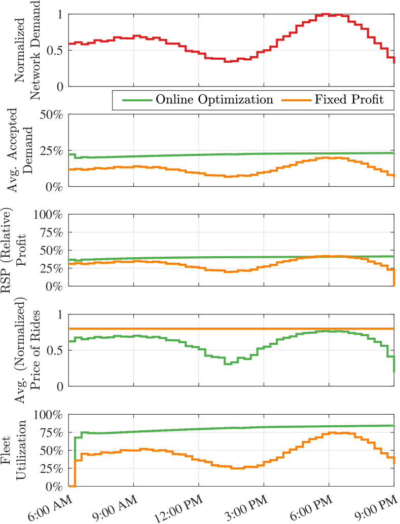
Figure 5: Comparison between optimized pricing policy and fixed-pricing policy. In the fixed-pricing policy, the RSP sets prices to guarantee a 25% profit from the operational cost of the fleet. All lines show trajectories averaged over 100 realizations of the simulation and over the regions of the network (Figure 3). Network demand data was derived from [45] for March 1, 2019, and normalized by its maximum value for illustration purposes. Fleet size was set to $25\%$ of the maximum demand. The RSP profit (third panel) was normalized by the maximum profit achievable if the fleet had an infinite number of vehicles.The average price of rides (fourth panel) was normalized by the maximum willingness to pay ${p}^{\textup{max}}$.

To solve the optimization problems we employ the projected controller (15) to account for constraints. All experiments were performed using Matlab 2019a, ride demands and locations were estimated by using the Taxi and Limousine Commission (TLC) data from New York City [45] for March 1, 2019 between 6:00AM and 9:00PM. Note that the available demand data does not describe the potential rides, but rather the realized ones. Although this data may not reflect the true demand, it is often used as a good approximation in several related works (see e.g., [43]).

Figure 4(a) illustrates the numerical tracking error and the error bound characterized in Theorem VI.1, and Figure 4(b) presents a breakdown of the terms characterizing the tracking error. The plots show that during the initial transient the tracking error quickly decreases, up to a steady-state value of order $10^{-2}$, thus validating the conclusions drawn in Theorem VI.1. Figure 4(b) showcases that the tracking error does not further decrease beyond such steady-state error because the optimizer $({u}^{\textup{so}}_{k},{x}^{\textup{so}}_{k})$ is changing over time. The sudden increase in error that occurs at around 1:00PM can be interpreted by means of Fig 3(b), which shows that the price of rides, at this time of the day, must decrease consistently since the network experiences a drop in ride demands (see Figure 5, top panel).

In Figure 5, we compare the performance of the online optimization method with a fixed-pricing policy, whereby the RSP selects a fixed price for all rides, corresponding to a 25% profit from the operational cost of the fleet. A 25% profit was selected as the maximum profit that allows the RSP to serve the peak of demand with the available fleet. Figure 5, second panel from the top, shows that by using the adaptive pricing policy the RSP always accept a higher number of rides; Figure 5, third panel, shows that the RSP profit is always higher under the adaptive pricing policy except at the peak of demand, which can be interpreted as an optimistic situation where suboptimal pricing still leads to a high utilization of the fleet; Figure 5, fourth panel shows that the adaptive policy adjusts the price of rides based on the instantaneous demand, and showcases that our optimal pricing policy tends to reduce the price of rides in the interest of maximizing fleet utilization; finally, Figure 5, bottom panel, shows that the optimized pricing policy always results in a higher fleet utilization.

VIII Conclusions

We have proposed a data-driven method to design controllers that steer an unknown dynamical system to the solution trajectory of a stochastic, time-varying optimization problem. The technique does not rely on any prior knowledge or estimation of the system matrices or the exogenous disturbances affecting the model equation. We have shown how knowledge of (possibly noisy) input-output data generated by the open-loop system can be used to compute the steady-state transfer function of the system and how to approximate it when disturbances are unknown. Our analysis has established that the resulting closed-loop dynamics are strictly contractive when the controller gain is chosen: (i) small enough so that the controller is sufficiently slower than the dynamical system and, simultaneously, (ii) large enough so that the controller can overcome shifts in the distributions associated with the lack of knowledge of the system dynamics. Our work here demonstrates for the first time that online optimization techniques can be used to control dynamical systems even when the system model is unknown. This opens up several exciting opportunities for future work, including extensions to scenarios where the control method guarantees persistence of excitation, and the generalization to scenarios with distributed computation, sensing, and communication.

References

- [1] G. Bianchin, M. Vaquero, J. Cortés, and E. Dall’Anese, “Data-driven synthesis of optimization-based controllers for regulation of unknown linear systems,” in IEEE Conf. on Decision and Control, Austin, TX, Dec. 2021, to appear.
- [2] A. Jokic, M. Lazar, and P. van den Bosch, “On constrained steady-state regulation: Dynamic KKT controllers,” IEEE Transactions on Automatic Control, vol. 54, no. 9, pp. 2250–2254, 2009.
- [3] F. Brunner, H.-B. Dürr, and C. Ebenbauer, “Feedback design for multi-agent systems: A saddle point approach,” in IEEE Conf. on Decision and Control, 2012, pp. 3783–3789.
- [4] M. Colombino, E. Dall’Anese, and A. Bernstein, “Online optimization as a feedback controller: Stability and tracking,” IEEE Transactions on Control of Network Systems, vol. 7, no. 1, pp. 422–432, 2020.
- [5] L. S. P. Lawrence, Z. E. Nelson, E. Mallada, and J. W. Simpson-Porco, “Optimal steady-state control for linear time-invariant systems,” in IEEE Conf. on Decision and Control, Dec. 2018, pp. 3251–3257.
- [6] A. Hauswirth, S. Bolognani, G. Hug, and F. Dörfler, “Timescale separation in autonomous optimization,” IEEE Transactions on Automatic Control, vol. 66, no. 2, pp. 611–624, 2021.
- [7] G. Bianchin, J. Cortés, J. I. Poveda, and E. Dall’Anese, “Time-varying optimization of LTI systems via projected primal-dual gradient flows,” arXiv preprint, Jan. 2021, arXiv:2101.01799.
- [8] M. Nonhoff and M. A. Müller, “Online gradient descent for linear dynamical systems,” arXiv preprint, 2019, arXiv:1912.09311.
- [9] G. Belgioioso, D. Liao-McPherson, M. H. de Badyn, S. Bolognani, J. Lygeros, and F. Dörfler, “Sampled-data online feedback equilibrium seeking: Stability and tracking,” arXiv preprint, 2021, arXiv:2103.13988.
- [10] S. Menta, A. Hauswirth, S. Bolognani, G. Hug, and F. Dörfler, “Stability of dynamic feedback optimization with applications to power systems,” in Annual Conf. on Communication, Control, and Computing, Oct. 2018, pp. 136–143.
- [11] G. Bianchin, E. Dall’Anese, J. I. Poveda, and A. Buchwald, “When can we safely return to normal? a novel method for identifying safe levels of npis in the context of covid-19 vaccinations,” medRxiv, 2021.
- [12] G. Bianchin, J. I. Poveda, and E. Dall’Anese, “Online optimization of switched LTI systems using continuous-time and hybrid accelerated gradient flows,” arXiv preprint, Aug. 2020, arXiv:2008.03903.
- [13] J. C. Willems, P. Rapisarda, I. Markovsky, and B. D. Moor, “A note on persistency of excitation,” Systems & Control Letters, vol. 54, no. 4, pp. 325–329, 2005.
- [14] T. Maupong and P. Rapisarda, “Data-driven control: A behavioral approach,” Systems & Control Letters, vol. 101, pp. 37–43, 2017.
- [15] C. D. Persis and P. Tesi, “Formulas for data-driven control: Stabilization, optimality and robustness,” IEEE Transactions on Automatic Control, vol. 65, no. 3, pp. 909–924, 2020.
- [16] S. Talebi, S. Alemzadeh, N. Rahimi, and M. Mesbahi, “Online regulation of unstable LTI systems from a single trajectory,” arXiv preprint, 2020, arXiv:2006.00125.
- [17] J. Coulson, J. Lygeros, and F. Dörfler, “Data-enabled predictive control: In the shallows of the DeePC,” in European Control Conference, 2019, pp. 307–312.
- [18] J. Berberich, J. Koehler, M. A. Müller, and F. Allgöwer, “Data-driven model predictive control with stability and robustness guarantees,” IEEE Transactions on Automatic Control, vol. 66, no. 4, pp. 1702–1717, 2021.
- [19] G. Baggio, V. Katewa, and F. Pasqualetti, “Data-driven minimum-energy controls for linear systems,” IEEE Control Systems Letters, vol. 3, no. 3, pp. 589–594, 2019.
- [20] L. Xu, M. Turan Sahin, B. Guo, and G. Ferrari-Trecate, “A data-driven convex programming approach to worst-case robust tracking controller design,” arXiv preprint, 2021, arXiv:2102.11918.
- [21] A. Allibhoy and J. Cortés, “Data-based receding horizon control of linear network systems,” IEEE Control Systems Letters, vol. 5, no. 4, pp. 1207–1212, 2020.
- [22] J. Berberich and F. Allgöwer, “A trajectory-based framework for data-driven system analysis and control,” in European Control Conference, 2020, pp. 1365–1370.
- [23] M. Guo, C. De Persis, and P. Tesi, “Data-driven stabilization of nonlinear polynomial systems with noisy data,” arXiv preprint, 2020, arXiv:2011.07833.
- [24] E. Hazan, “Introduction to online convex optimization,” Foundations and Trends in Optimization, vol. 2, no. 3-4, pp. 157–325, 2016.
- [25] S. Bolognani and S. Zampieri, “A distributed control strategy for reactive power compensation in smart microgrids,” IEEE Transactions on Automatic Control, vol. 58, no. 11, pp. 2818–2833, 2013.
- [26] A. Bernstein, E. Dall’Anese, and A. Simonetto, “Online primal-dual methods with measurement feedback for time-varying convex optimization,” IEEE Transactions on Signal Processing, vol. 67, no. 8, pp. 1978–1991, 2019.
- [27] C.-Y. Chang, M. Colombino, J. Cortés, and E. Dall’Anese, “Saddle-flow dynamics for distributed feedback-based optimization,” IEEE Control Systems Letters, vol. 3, no. 4, pp. 948–953, 2019.
- [28] D. Li, D. Fooladivanda, and S. Martínez, “Online optimization and learning in uncertain dynamical environments with performance guarantees,” arXiv preprint, 2021, arXiv:2102.09111.
- [29] K. Hirata, J. Hespanha, and K. Uchida, “Real-time pricing leading to optimal operation under distributed decision makings,” in American Control Conference, 2014, pp. 1925–1932.
- [30] M. Nonhoff and M. A. Müller, “Data-driven online convex optimization for control of dynamical systems,” arXiv preprint, 2021, arXiv:2103.09127.
- [31] J. C. Perdomo, T. Zrnic, C. Mendler-Dünner, and M. Hardt, “Performative prediction,” arXiv preprint, 2021, arXiv:2002.06673.
- [32] C. Mendler-Dünner, J. C. Perdomo, T. Zrnic, and M. Hardt, “Stochastic optimization for performative prediction,” arXiv preprint, 2020, arXiv:2006.06887.
- [33] D. Drusvyatskiy and L. Xiao, “Stochastic optimization with decision-dependent distributions,” arXiv preprint, 2020, arXiv:2011.11173.
- [34] M. Yin, A. Iannelli, and R. S. Smith, “Maximum likelihood estimation in data-driven modeling and control,” arXiv preprint, 2020, arXiv:2011.00925.
- [35] H. J. van Waarde, M. K. Camlibel, and M. Mesbahi, “From noisy data to feedback controllers: non-conservative design via a matrix S-lemma,” IEEE Transactions on Automatic Control, 2021, in press.
- [36] A. Bisoffi, C. De Persis, and P. Tesi, “Trade-offs in learning controllers from noisy data,” arXiv preprint, 2021, arXiv:2103.08629.
- [37] S. Bubeck, “Convex optimization: Algorithms and complexity,” Foundations and Trends Machine Learning, vol. 8, no. 3–4, p. 231–357, Nov. 2015.
- [38] L. V. Kantorovich and S. G. Rubinshtein, “On a space of totally additive functions,” Vestnik Leningradskogo Universiteta, vol. 13, no. 7, pp. 52–59, 1958.
- [39] E. Davison, “The robust control of a servomechanism problem for linear time-invariant multivariable systems,” IEEE Transactions on Automatic Control, vol. 21, no. 1, pp. 25–34, 1976.
- [40] S. Boyd and L. Vandenberghe, Convex Optimization. Cambridge University Press, 2004.
- [41] H. Karimi, J. Nutini, and M. Schmidt, “Linear convergence of gradient and proximal-gradient methods under the Polyak-Łojasiewicz condition,” in Joint European Conference on Machine Learning and Knowledge Discovery in Databases, 2016, pp. 795–811.
- [42] A. Khaled and P. Richtárik, “Better theory for SGD in the nonconvex world,” arXiv preprint, 2020, arXiv:2002.03329.
- [43] B. Turan and M. Alizadeh, “Competition in electric autonomous mobility on demand systems,” IEEE Transactions on Control of Network Systems, 2021, in press.
- [44] W. M. Haddad, V. S. Chellaboina, and E. August, “Stability and dissipativity theory for discrete-time non-negative and compartmental dynamical systems,” International Journal of Control, vol. 76, no. 18, pp. 1845–1861, 2003.
- [45] “TLC trip record data,” https://www1.nyc.gov/site/tlc/about/tlc-trip-record-data.page, [Online; accessed 12-Aug-2021].