Shatter: An Efficient Transformer Encoder with Single-Headed Self-Attention and Relative Sequence Partitioning

Abstract

The highly popular Transformer architecture, based on self-attention, is the foundation of large pretrained models such as BERT, that have become an enduring paradigm in NLP. While powerful, the computational resources and time required to pretrain such models can be prohibitive. In this work, we present an alternative self-attention architecture, Shatter, that more efficiently encodes sequence information by softly partitioning the space of relative positions and applying different value matrices to different parts of the sequence. This mechanism further allows us to simplify the multi-headed attention in Transformer to single-headed. We conduct extensive experiments showing that Shatter achieves better performance than BERT, with pretraining being faster per step (15% on TPU), converging in fewer steps, and offering considerable memory savings (>50%). Put together, Shatter can be pretrained on 8 V100 GPUs in 7 days, and match the performance of BERT_Base – making the cost of pretraining much more affordable.

1 Introduction

Large pretrained models such as BERT (Devlin et al., 2019) have become a mainstay of natural language processing (NLP), enabling the transfer of knowledge learned from large amounts of unsupervised data to downstream tasks with a small number of labeled examples. Due to the size of both the unsupervised data and model architecture, pretraining is computationally very expensive, requiring either TPUs or a substantial number of GPUs (Liu et al., 2019), which can make experimentation cumbersome. As a result, many have attempted to improve pretraining efficiency from largely two aspects: the model architecture (Ke et al., 2020; Shaw et al., 2018; He et al., 2020) or pretraining objective (Yang et al., 2019; Clark et al., 2020).

In this work, we focus on developing a more efficient architecture, inspired by the recent literature of modeling sequence attention with relative position embeddings (Shaw et al., 2018). Similar techniques have been integrated in many Transformer variants (Yang et al., 2019; Raffel et al., 2019; He et al., 2020; Ke et al., 2020), and as we show in this work, relative position embeddings not only achieve better finetuned performance with fewer pretraining steps (§5.2), but also hold the potential of being pretrained on shorter sequences than used in finetuning, which could considerably reduce the memory requirements and accelerate pretraining.

Unfortunately, training with relative position embeddings is much slower per step: While Shaw et al. (2018) reported $7\%$ more training time on GPUs, we found it $3.9$ times slower than BERT on TPUs (§5.1). Consequently, the cost in speed hinders the adoption of this model.

In this work, we develop an alternative that captures the advantages of relative position embeddings (i.e. better finetuning performance with fewer pretraining steps, pretraining on shorter sequence length) without the associated speed overhead. Instead of using (absolute or relative) position embeddings, we propose to incorporate sequence order information by softly partitioning the space of relative positions into parts, which can be implemented by a TPU-efficient operation of multiplying the attention matrix with a constant mask.

Subsequently, we can replace multi-headed attention with a single-headed variant, by changing the activation function from softmax (i.e. L1-normalized $\exp$ which favors sparse positions of the top attention score) to L2-normalized sigmoid (which favors dense weighting of positions). This single-headed formulation simplifies the concept of self-attention, and leads to further efficiency gains.

We exhaustively evaluate our model, Shatter, across several datasets: The GLUE Benchmark (Wang et al., 2018), SQuAD (Rajpurkar et al., 2016), BoolQ (Clark et al., 2019) and MultiRC (Khashabi et al., 2018). We show that our model is 15% faster per pretraining step than BERT on TPU (§5.1), and achieves better finetuned performance across the datasets, for both base and large size, with fewer pretraining steps (§5.2.3). Furthermore, we show that our approach generalizes better to longer sequences, and can pretrain on half the sequence length required in finetuning, which reduces the memory footprint by more than 50% (§5.2.2). Put together, we can pretrain the base-size Shatter on 8 V100 GPUs in 7 days and match or outperform BERT_Base, significantly reducing the computational requirements for pretraining.

2 Background

A Transformer encoder (Vaswani et al., 2017) is a stack of self-attention (Cheng et al., 2016; Parikh et al., 2016) and feed-forward layers. In the following, we briefly review the self-attention mechanism and some variants to model relative position. Vectors are denoted by lowercase bold letters, matrices by uppercase bold, and tensors of higher ranks by bold sans-serif. We use Numpy indexing for tensors, and matrices are row-major.

At each layer $k$, the hidden state of a Transformer is represented by an $l\times d$ matrix ${\bm{X}}^{k}$, where $l$ is the sequence length and $d$ the hidden size. For simplicity of notation, we omit the $k$ superscript unless the layer index is critical. The hidden vector ${\bm{x}}_{i}={\bm{X}}[i,:]$ $(0\leq i<l)$ encodes context around position $i$ in the sequence.

From the hidden state, self-attention calculates the query ${\bm{Q}}$, key ${\bm{K}}$, and value ${\bm{V}}$ matrices as trainable linear transformations of ${\bm{X}}$:

$${\bm{Q}} ={\bm{X}}{\bm{W}}^{Q},\;{\bm{K}}={\bm{X}}{\bm{W}}^{K},\;{\bm{V}}={\bm{X}}{\bm{W}}^{V}$$

Then, it uses query and key to compute attention scores and construct a weighted average of the value:

$${\bm{A}} =\mathrm{softmax}\left(\frac{{\bm{Q}}{\bm{K}}^{\top}}{\sqrt{d}}\right)$$

$$\bar{{\bm{X}}} ={\bm{A}}{\bm{V}}$$

Here, ${\bm{A}}$ is an $l\times l$ matrix, with ${\bm{A}}[i,j]$ representing the attention score from position $i$ to position $j$. The input to the next layer ${\bm{X}}^{k+1}$ is computed as $F^{k}(\bar{{\bm{X}}}^{k},{\bm{X}}^{k})$, where $F^{k}$ is a feed forward network with layer normalization (Ba et al., 2016).

Multi-headed Attention

In practice, it performs better to divide the inner dimension of ${\bm{Q}}$, ${\bm{K}}$ and ${\bm{V}}$ into $n$ blocks, and run the self-attention mechanism $n$ times in parallel. This is calculated formally by converting ${\bm{Q}}$ into a rank $3$ tensor ${\bm{\mathsfit{Q}}}$ such that:

$${\bm{\mathsfit{Q}}}[h,:,:]={\bm{Q}}[:,\tfrac{h}{n}d:\tfrac{h+1}{n}d]\quad(0\leq h<n)$$

and similarly ${\bm{K}}$, ${\bm{V}}$ into ${\bm{\mathsfit{K}}}$, ${\bm{\mathsfit{V}}}$, respectively. Then, multi-headed attention is computed by:

$${\bm{\mathsfit{A}}} =\mathrm{softmax}\left(\frac{{\bm{\mathsfit{Q}}}{\bm{\mathsfit{K}}}^{\top}}{\sqrt{d/n}}\right)$$ (1)

$$\bar{{\bm{\mathsfit{X}}}} ={\bm{\mathsfit{A}}}{\bm{\mathsfit{V}}}$$ (2)

where multiplication of tensors means batched matrix multiplication. The tensor $\bar{{\bm{\mathsfit{X}}}}$ is converted back to a matrix $\bar{{\bm{X}}}$ by setting

$$\bar{{\bm{X}}}[:,\tfrac{h}{n}d:\tfrac{h+1}{n}d]=\bar{{\bm{\mathsfit{X}}}}[h,:,:]\quad(0\leq h<n).$$ (3)

Here, ${\bm{\mathsfit{A}}}$ is a $n\times l\times l$ tensor, where each “attention head” ${\bm{\mathsfit{A}}}[h,:,:]$ is expected to weight sequence positions from different aspects, and the model more efficiently encodes context information.

Position Embeddings

Self-attention does not recognize sequence order; i.e., a permutation of rows in ${\bm{X}}$ leads to the same permutation of rows in $\bar{{\bm{X}}}$. To inject order information, Transformer learns an $l\times d$ matrix ${\bm{P}}$ as “position embeddings”, besides the word embeddings ${\bm{E}}$. Namely, given a word sequence $w_{0}w_{1}\ldots$ of length $l$, the input vector ${\bm{x}}^{0}_{i}$ of the first layer is calculated by:

$${\bm{x}}^{0}_{i}=\operatorname{LayerNormalize}({\bm{E}}(w_{i})+{\bm{P}}[i]).$$ (4)

Thus, a permutation of the word sequence $w_{0}w_{1}\ldots$ does not lead to a permutation of rows in ${\bm{X}}^{0}$, thanks to position embeddings.

Relative Position Embeddings

Although being simple, position embeddings only inject order information to the first layer, and the solution is not shift-invariant (e.g., if we shift $w_{0}w_{1}\ldots$ one position to the right, the input sequence $\texttt{<pad>}w_{0}w_{1}\ldots$ will be encoded into completely different hidden states, not the shift of hidden states of $w_{0}w_{1}\ldots$, which is unintuitive of a sequence encoder). As an alternative, the Relative Position Embeddings (RPE) model (Shaw et al., 2018) aims to inject stronger notion of position at each self-attention layer, with shift-invariance. The model learns a $(2l-1)\times d$ matrix ${\bm{R}}^{k}$ at each layer $k$, which contributes to both attention scores and values, as below:

$${\bm{S}}={\bm{Q}} {\bm{K}}^{\top},\;{\bm{S}}_{\text{rel}}[i,j-i]={\bm{S}}[i,j]$$

$${\bm{K}}_{\text{rel}} ={\bm{R}}{\bm{W}}^{K},\;{\bm{V}}_{\text{rel}}={\bm{R}}{\bm{W}}^{V}$$

$${\bm{A}}_{\text{rel}} =\mathrm{softmax}\left(\frac{{\bm{S}}_{\text{rel}}+{\bm{Q}}{\bm{K}}_{\text{rel}}^{\top}}{\sqrt{d}}\right)$$

$${\bm{A}}[i,j] ={\bm{A}}_{\text{rel}}[i,j-i]$$

$$\bar{{\bm{X}}} ={\bm{A}}{\bm{V}}+{\bm{A}}_{\text{rel}}{\bm{V}}_{\text{rel}}$$

Here, ${\bm{S}}_{\text{rel}}$ and ${\bm{A}}_{\text{rel}}$ are $l\times(2l-1)$ matrices with inner index ranging from $-l+1$ to $l-1$, representing attention to relative positions. Intuitively, the calculation corresponds to using ${\bm{x}}_{j}+{\bm{R}}[j-i]$ to obtain key and value, while using ${\bm{x}}_{i}$ to obtain query. The multi-headed case is defined similarly.

In the above calculation, RPE requires conversion between ${\bm{S}},{\bm{A}}$ and ${\bm{S}}_{\text{rel}},{\bm{A}}_{\text{rel}}$, respectively, which changes the memory configuration of these tensors in the accelerator in a less optimized manner, and increases computational cost. This is especially a bottleneck on TPUs, making the model difficult to scale up to larger size.

Nevertheless, RPE consistently performs better in our experiments (§5.2), and the model can be naturally extended to longer sequences by copying the learnt embeddings ${\bm{R}}[-l+1]$ and ${\bm{R}}[l-1]$ to farther relative positions. It serves as a strong motivation for us to design a fast alternative for relative position modeling.

Relative Attention Bias

Several Transformer variants (Raffel et al., 2019; He et al., 2020; Ke et al., 2020) have simplified the relative position modeling, in addition to the (absolute) position embeddings. For example, instead of Eq.1, the T5 model (Raffel et al., 2019) learns an attention bias ${\bm{\mathsfit{B}}}$ according to relative positions:

$${\bm{\mathsfit{B}}}[:,i,j] ={\bm{W}}^{B}[g,:]\quad(b_{g}\leq j-i<b_{g+1})$$

$${\bm{\mathsfit{A}}} =\mathrm{softmax}\left(\frac{{\bm{\mathsfit{Q}}}{\bm{\mathsfit{K}}}^{\top}}{\sqrt{d/n}}+{\bm{\mathsfit{B}}}\right)$$

In which, ${\bm{\mathsfit{B}}}$ is an $n\times l\times l$ tensor obtained from a trainable $m\times n$ matrix ${\bm{W}}^{B}$, with the relative position $j-i$ put into one of $m$ fixed buckets: $b_{0}=-\infty<\ldots b_{g}\ldots<b_{m}=\infty$. The computation of this Relative Attention Bias (RAB) model is much simpler than RPE, but still adds extra cost. In our experiments, using the T5 default $m=32$, pretraining RAB is $20\%$ more costly than the vanilla Transformer on TPU. Performance is improved on some tasks, but not all (§5.2.1).

3 Our Approach

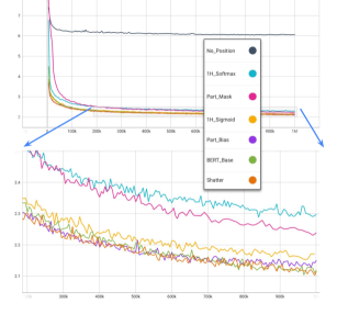
Figure 1: The learning curves (MLM valid loss over pretraining step) of our model variants, developed one by one and lead to Shatter, compared with BERT_Base.

In this section, we describe the components of our more efficient self-attention architecture, Shatter, by steps. First, we partition the space of relative positions to softly bias each attention head to focus on a different part of the sequence (§3.1). Then, we can simplify the multi-head attention to single-headed (§3.2). Finally, we show how to incorporate partition embeddings for improved performance with minimal additional cost ( §3.3).

A demonstrating experiment is shown in Figure 1: We progressively develop our model variants and show their Masked Language Modeling (MLM) loss Devlin et al. (2019) on a validation corpus during pretraining. Detailed settings are given in §A.2. The baseline is BERT_Base, and we note its learning curve converging to $\approx\!2$ (Figure 1, “BERT_Base”). We start from removing the position embeddings in Eq.4, and the valid loss drastically increases to $>\!6$ (Figure 1, “No_Position”), which suggests that the sequence order information is crucial for a Transformer encoder.

3.1 Soft Relative Partition of Sequence

Instead of position embeddings, we explore an alternative way of integrating sequence order, by restricting different attention heads to different parts of a sequence. This is achieved by multiplying a mask ${\bm{\mathsfit{N}}}$ to the attention score:

$${\bm{\mathsfit{A}}} =\mathrm{softmax}\left(\frac{{\bm{\mathsfit{Q}}}{\bm{\mathsfit{K}}}^{\top}}{\sqrt{d/n}}\right)\odot{\bm{\mathsfit{N}}}.$$ (5)

Here, $\odot$ denotes element-wise multiplication, and ${\bm{\mathsfit{N}}}$ is an $n\times l\times l$ constant tensor up to model design. Intuitively, the attention head $h$ at position $i$ is more sensitive to position $j$ if ${\bm{\mathsfit{N}}}[h,i,j]$ is larger. We set ${\bm{\mathsfit{N}}}$ to be dependent only on the relative position $j-i$, which makes the model shift-invariant:

$${\bm{\mathsfit{N}}}[h,i,j]=f_{h}(j-i).$$

In order to recognize sequence order, $f_{h}$ should not be constant; we use a partition of unity to evenly concentrate different $f_{h}$ to different parts of the relative position space.

A partition of unity is a group of functions $\{f_{h}\}$ $(0\leq h<n)$ such that: (i) $f_{h}(x)\geq 0$ and (ii) $\sum_{h=0}^{n-1}f_{h}(x)=1$, for any $x\in(-\infty,\infty)$. For example, consider the four functions in Figure 2: $f_{0}$ concentrates at relative position $j-i=x=1$ and $f_{2}$ peaks around $j-i=x=4$, while $f_{0}+f_{1}+f_{2}+f_{3}$ constantly equals $1$ at all positions.

The partition of unity is a generalization of T5’s idea of putting relative positions into buckets: Dividing $(-\infty,\infty)$ into $n$ buckets, $b_{0}=-\infty<\ldots b_{h}\ldots<b_{n}=\infty$, is equivalent to setting

$$f_{h}(x)=\begin{cases}1\quad\mbox{If $b_{h}\leq x<b_{h+1}$}\\ 0\quad\mbox{Otherwise}\end{cases}.$$

In our case, instead of a hard division into buckets, we adopt a soft division to avoid discontinuity at bucket boundaries. Specifically, we use Bernstein polynomials to construct the partition of unity, and the detailed definition is given in §A.1.

Compared to Eq.1, the extra computation cost of Eq.5 is negligible, because ${\bm{\mathsfit{N}}}$ is constant without any trainable components. Figure 1 (“Part_Mask”) shows that multiplying ${\bm{\mathsfit{N}}}$ largely closes the gap between BERT_Base and “No_Position”.

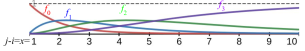
Figure 2: An illustration of the partition of unity used in this work, which consists of four functions {$f_{0}$, $f_{1}$, $f_{2}$, $f_{3}$} over the relative position space.

3.2 One-Head Sigmoid Attention

The partition mask ${\bm{\mathsfit{N}}}$ makes different attention heads focus on different parts of the sequence, limiting the overlap between parts. It suggests a possibility to neatly combine all the attention scores over the whole sequence into one $l\times l$ matrix, without the multi-headed redundancy. Formally, it suggests that we may replace the tensor ${\bm{\mathsfit{Q}}}{\bm{\mathsfit{K}}}^{\top}$ with the matrix version ${\bm{Q}}{\bm{K}}^{\top}$, without loss of model expressivity. For the matrix version, linear algebra suggests that we may further replace ${\bm{K}}={\bm{X}}{\bm{W}}^{K}$ by ${\bm{X}}$, which reduces one matrix multiplication for the self-attention layer. It leads to $5\%$ reduction of training time on GPU and $15\%$ on TPU, in our experiments (§5.1).

One issue with the matrix version (i.e. single-headed attention), is that attention scores are calculated by softmax (i.e. L1-Normalized $\exp$), which favors sparse positions of the top attention score; it might still be better to attend to more positions, as in multi-headed attention. Thus, we propose to use L2-Normalized sigmoid instead of softmax, which favors a dense weighting of positions:

$${\bm{\mathsfit{A}}} =\operatorname{L2-Normalize}\left(\sigma\left(\frac{{\bm{Q}}{\bm{X}}^{\top}}{\sqrt{d}}\right)\right)\odot{\bm{\mathsfit{N}}}.$$ (6)

Figure 1 shows the effect of single-headed attention: If we use softmax scores (“1H_Softmax”), the validation loss gets slightly worse; however, it is significantly improved by using L2-Normalized sigmoid (“1H_Sigmoid”).

It is noteworthy that in Eq.6, although ${\bm{Q}}{\bm{X}}^{\top}$ is a matrix, we still get an $n\times l\times l$ tensor ${\bm{\mathsfit{A}}}$ by multiplying to ${\bm{\mathsfit{N}}}$ through Numpy broadcasting. We use Eq.6 to replace Eq.1, then the tensor $\bar{{\bm{\mathsfit{X}}}}={\bm{\mathsfit{A}}}{\bm{\mathsfit{V}}}$ is calculated the same as in Eq.2. It is crucial to keep ${\bm{\mathsfit{V}}}$ as a rank 3 tensor to make the model aware of different parts of the sequence. We have confirmed in preliminary experiments, that reducing ${\bm{\mathsfit{V}}}$ to matrix would hurt valid loss, even with sigmoid attention score.

3.3 Partition Embeddings

Besides injecting sequence order, (absolute or relative) position embeddings enable a model to attend to a position no matter what the token is. To achieve a similar role, we further add partition embeddings to our final model, named Shatter (Single-headed attention with relative partition).

At each layer, Shatter learns an $n\times d$ matrix ${\bm{R}}$ to represent partition, in analogue to the relative position embeddings. It uses the query ${\bm{Q}}$, partition embeddings ${\bm{R}}$, and the partition mask ${\bm{\mathsfit{N}}}$ to calculate an attention bias ${\bm{B}}$ as the following:

$${\bm{B}}[i,:]=\sum_{h=0}^{n-1}({\bm{Q}}{\bm{R}}^{\top})[i,h]\cdot{\bm{\mathsfit{N}}}[h,i,:]$$

$${\bm{\mathsfit{A}}}=\operatorname{L2-Normalize}\left(\sigma\left(\frac{{\bm{Q}}{\bm{X}}^{\top}}{\sqrt{d}}+{\bm{B}}\right)\right)\odot{\bm{\mathsfit{N}}}$$

In addition, ${\bm{R}}$ contributes to the value as below:

$${\bm{A}}_{\text{part}}^{\top}=\sum_{j=0}^{l-1}{\bm{\mathsfit{A}}}[:,:,j],\;{\bm{V}}_{\text{part}}={\bm{R}}{\bm{W}}^{V}$$

$$\bar{\bar{{\bm{X}}}}=\bar{{\bm{X}}}+{\bm{A}}_{\text{part}}{\bm{V}}_{\text{part}}$$

where $\bar{{\bm{X}}}$ is defined the same as in Eq.3. Then, $\bar{\bar{{\bm{X}}}}$ is used in the feed-forward network instead of $\bar{{\bm{X}}}$.

In Figure 1, “Part_Bias” shows the effect of adding the bias term ${\bm{B}}$, and “Shatter” shows the result adding value contribution. Our final model now matches the valid loss of BERT_Base.

The computation cost of partition embeddings is small, because $n\ll l$, and the part-wise bias for the attention score is converted to absolute positions via matrix multiplication by a constant tensor ${\bm{\mathsfit{N}}}$, without memory rearrangement.

3.4 Sequence Classification with Relative Position Modeling

Model	Size	# Params	Hardware	Batch	Length	# Steps	Time
BERTGPU	12-layers 12-heads 768-hidden	84.9M	GPU V100$\times 8$	128	256	1.6M	170 hrs
ShatterGPU	12-layers 12-parts 768-hidden	78.0M	GPU V100$\times 8$	128	256	1.6M	161 hrs
BERTBase	12-layers 12-heads 768-hidden	84.9M	TPUv3 4x4	256	512	1M	53 hrs
ShatterBase	12-layers 12-parts 768-hidden	78.0M	TPUv3 4x4	256	512	1M	45 hrs
BERT-RPE	12-layers 12-heads 768-hidden	87.3M	TPUv3 4x4	256	512	1M	206 hrs
BERT-RAB	12-layers 12-heads 768-hidden	84.9M	TPUv3 4x4	256	512	1M	64 hrs
XLNetBase	12-layers 12-heads 768-hidden	92.0M	TPUv3 4x4	256	512	1M	123 hrs
BERTLarge	24-layers 16-heads 1024-hidden	151.0M	TPUv3 8x8	1024	512	1M	180 hrs
ShatterLarge	24-layers 16-parts 1024-hidden	138.6M	TPUv3 8x8	1024	512	1M	151 hrs

Table 1: Number of trainable parameters (excluding word embeddings), pretraining settings and pretraining speed.

For sequence classification tasks, BERT adds [CLS] and [SEP] tokens to the input sequence(s) and feeds the final hidden state at [CLS] to a classifier. As pointed out by Ke et al. (2020), this strategy might hurt models using relative position, since the hidden state at [CLS] might be affected by its position relative to other tokens, which is irrelevant to [CLS]’s role of capturing the semantics of the whole sequence(s). Therefore, Ke et al. (2020) propose a mechanism to “reset” relative positions regarding [CLS], but this mechanism is model specific. Related to the issue, He et al. (2020) propose to model relative positions but add absolute position embeddings to the last few layers.

In this work, we adopt a modified strategy for sequence classification, and apply it to all sequence encoders in our experiments for fair comparison. We first encode [CLS]- and [SEP]- augmented input sequence(s) and record the hidden state ${\bm{X}}^{k}$ at each layer $(0\leq k\leq L)$. Then, instead of using [CLS]’s final hidden state ${\bm{X}}^{L}[0,:]$, we newly start from a learnt vector ${\bm{y}}^{0}$ and recalculate a weighted average of the hidden states at each layer:

$${\bm{q}} ={\bm{y}}{\bm{W}}^{Q},\;{\bm{K}}={\bm{X}}{\bm{W}}^{K},\;{\bm{V}}={\bm{X}}{\bm{W}}^{V}$$

$${\bm{a}} =\mathrm{softmax}\left(\frac{{\bm{q}}{\bm{K}}^{\top}}{\sqrt{d}}\right),\;\bar{{\bm{y}}}={\bm{a}}{\bm{V}}$$

Finally, the result ${\bm{y}}^{L}$ is used for classification. In the above, the attention mechanism is replaced with either multi-headed or single-headed sigmoid, according to the sequence encoder model.

Our experiments suggest that the strategy does not affect the performance of BERT, but improves others that model relative positions (§A.4).

4 Related Work

The original Transformer (Vaswani et al., 2017) uses fixed sinusoid functions to encode positions, justified by the existence of linear transformations between vectors of different positions. This idea is conveyed further by XLNet (Yang et al., 2019), which models relative positions (hence shift-invariant) and can accumulate context information of arbitrary length. Our relative sequence partitioning method differs by directly affecting the attention score, and the coarse partition imposes more regularization than position-wise vectors. We will further compare with XLNet in our evaluation.

BERT (Devlin et al., 2019) learns the position embeddings, and Shaw et al. (2018) model relative positions. Many (Raffel et al., 2019; He et al., 2020; Ke et al., 2020; Wennberg and Henter, 2021; Chen et al., 2021) combine the techniques with different approaches, while we point out that modeling relative positions with learnt components often increases pretraining cost, and will clearlly evaluate the cost-performance trade-off.

Many ideas are explored to reduce the training cost (Lan et al., 2019; Jiang et al., 2020; Chen et al., 2020; Lee-Thorp et al., 2021), some specifically for very long ($\geq\!4096$) sequences (Child et al., 2019; Kitaev et al., 2020; Choromanski et al., 2020; Beltagy et al., 2020), but we are not aware of previous work that can pretrain with 8 V100 GPUs within 1 week and match BERT_Base.

Previous works have found that multiple attention heads are redundant and can be pruned (Michel et al., 2019; Voita et al., 2019), but incorporating this insight into training is more challenging, as naively reducing the number of heads will reduce performance. Our single-headed self-attention both simplified the concept and improved performance.

5 Experiments

	CoLA		SST-2		MRPC		QQP		STS-B		MNLI-m		MNLI-mm		QNLI		RTE
	Dev. (Acc.)	Test (MCC)	Dev. (Acc.)	Test (Acc.)	Dev. (F1)	Test (F1)	Dev. (F1)	Test (F1)	Dev. ($\rho$)	Test ($\rho$)	Dev. (Acc.)	Test (Acc.)	Dev. (Acc.)	Test (Acc.)	Dev. (Acc.)	Test (Acc.)	Dev. (Acc.)	Test (Acc.)
BERTGPU 256-$l$	82.0	-	92.5	-	90.5	-	87.2	-	84.5	-	83.5	-	84.2	-	90.8	-	66.4	-
BERTGPU 512-$l$ ext.	82.1	-	92.8	-	86.1	-	86.7	-	84.5	-	82.9	-	83.2	-	90.1	-	63.9	-
ShatterGPU 512-$l$ ext.	83.3	49.1	92.2	92.5	91.3	88.7	87.8	70.6	85.5	85.1	84.5	84.2	84.8	83.6	91.4	90.4	66.1	65.4
BERTBase	83.6	46.9	92.2	92.3	89.7	87.6	87.3	70.2	85.6	83.8	84.0	83.5	83.8	82.4	90.7	89.8	65.3	61.8
ShatterBase	84.0	48.8	93.6	92.8	92.1	88.1	87.6	70.5	85.8	81.6	84.8	84.7	84.9	83.7	90.7	90.9	67.9	66.4
BERT-RPE	84.4	55.7	93.5	94.0	92.1	89.5	88.5	71.0	86.4	85.0	86.2	86.1	86.1	85.0	92.3	92.1	74.0	70.4
BERT-RAB	76.2	33.4	92.4	92.7	88.3	86.3	86.7	69.1	84.3	80.2	85.1	84.4	85.0	84.2	91.2	90.6	65.0	61.7
XLNetBase	79.4	-	93.0	-	90.8	-	86.4	-	81.8	-	84.1	-	84.6	-	89.6	-	68.2	-
Huggingface BERT	83.3	-	92.4	-	91.2	-	88.1	-	86.7	-	84.9	-	84.7	-	91.5	-	70.8	-
BERTLarge	84.9	56.5	95.4	94.2	92.4	90.1	88.4	71.6	87.3	85.9	88.9	88.2	88.8	87.4	93.6	93.0	80.9	75.4
ShatterLarge	85.9	65.2	96.2	95.6	93.3	90.4	88.7	71.2	87.9	90.3	88.7	88.4	88.6	87.6	94.1	93.3	84.1	77.0
BERTLarge 400k	81.2	44.5	93.9	94.7	91.3	84.7	88.3	71.5	86.9	85.6	87.6	87.2	87.6	86.2	93.2	92.5	70.0	63.5
ShatterLarge 400k	85.5	59.8	95.0	94.1	90.3	88.9	88.8	71.5	87.3	89.0	87.6	87.5	87.7	86.6	93.6	93.0	70.0	66.7
Jacob Devlin Subm.	-	60.5	-	94.9	-	89.3	-	72.1	-	86.5	-	86.7	-	85.9	-	92.7	-	70.1

Table 2: Results on GLUE. Test performance obtained by submitting to https://gluebenchmark.com/.

For evaluation, we implemented and compared the following models:

BERT (Devlin et al., 2019) is a Transformer encoder (Vaswani et al., 2017) with model parameters trained on large amounts of unsupervised data (i.e. pretraining). The Masked Language Modeling (MLM) pretraining objective attempts to recover the original tokens when 15% tokens in an input sequence are masked out. We pretrain three models, BERT_GPU, BERT_Base and BERT_Large, using different model size (Base or Large), sequence length (256-$l$ or 512-$l$) and hardware (GPU or TPU).

Shatter is our proposed model architecture. We pretrain Shatter_GPU, Shatter_Base and Shatter_Large, in correspondence to the BERT models.

BERT-RPE (Shaw et al., 2018) uses Relative Position Embeddings (RPE) at each layer, instead of (absolute) position embeddings. We set the vocab size of RPE to $2\times 128-1=255$, so that relative positions farther than $128$ are represented by the same embedding vector.

BERT-RAB adds a Relative Attention Bias (RAB) to the BERT model. Relative positions are put into buckets, and each bucket shares the same bias term. We copied code from the T5 model (Raffel et al., 2019) to implement bucketing, and the number of buckets is set to $32$ (T5 default).

XLNet (Yang et al., 2019) uses fixed sinusoid encoding to represent relative positions, and has a memorization mechanism to accumulate context information of arbitrary length. It is also pretrained by an auto-regressive Permutation Language Modeling (PLM) objective instead of MLM. In this work, we pretrain XLNet with PLM but without memorization, in order to adopt the same input data pipeline as other models.

All the models were implemented by modifying the code of Huggingface Transformers package (Wolf et al., 2020), using TensorFlow 2. We use the BooksCorpus (Zhu et al., 2015) and English Wikipedia to pretrain the models, the same as Devlin et al. (2019) (but not the same as RoBERTa (Liu et al., 2019)). More detailed settings for pretraining are given in §A.2.

5.1 Pretraining Cost

Table 1 shows the number of trainable parameters, and the time required to pretrain the models on different hardware. Shatter has a significant reduction in number of parameters than other models, due to the omission of a $d\times d$ matrix per layer (§3.2). It also leads to 5% faster pretraining speed than BERT on GPUs and 15% on TPUs.

Reducing the batch size to 128 and sequence length to 256 (the largest possible to fit in memory), we can pretrain Shatter on 8 V100 GPUs for 1.6M steps within 1 week. At step 1.6M, Shatter_GPU sees the same amount of tokens as Shatter_Base at step 400k; as we will show in §5.2.1, it is already close to converge and outperforms BERT_Base on GLUE.

BERT-RPE has significantly more parameters than BERT_Base, due to the relative position embeddings at each layer; which prevents the model from running on GPUs using the same settings as BERT_GPU. It is also $3.9$ times slower than BERT on TPUs, making it impractical to scale up to larger size. BERT-RAB has almost the same number of parameters as BERT, but still 20% slower on TPU; The most memory intensive model is XLNet, due to an extra trainable $d\times d$ matrix at each layer to transform the sinusoid encoding of relative positions. Pretraining of XLNet_Base is also slow, probably due to the two-stream self-attention calculation for the PLM objective.

5.2 Finetuning Results

We finetune the models on GLUE (Wang et al., 2018), SQuAD v1.1 (Rajpurkar et al., 2016), and MultiRC (Khashabi et al., 2018) and BoolQ (Clark et al., 2019) from SuperGLUE (Wang et al., 2019). For all tasks, we use the Adam optimizer (Kingma and Ba, 2014), set batch size to 16, evaluate the model in every 1k steps and choose the one that scores highest on the development set.

5.2.1 GLUE Benchmark

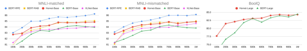
Figure 3: Plots showing finetuned performance on dev set (y-axis) as a function of pretrained steps (x-axis).

GLUE is a collection of classification tasks on text sequences or sequence pairs. Following Devlin et al. (2019), we evaluate on CoLA (Warstadt et al., 2019), SST-2 (Socher et al., 2013), MRPC (Dolan and Brockett, 2005), QQP, STS-B (Cer et al., 2017), MNLI (Williams et al., 2018), QNLI (Wang et al., 2018) and RTE (Bentivogli et al., 2009) in GLUE. Table 2 shows the results.

For BERT_Base, Devlin et al. (2019) finetuned with learning rate [1e-5, 2e-5, 3e-5, 4e-5, 5e-5] and took the best. We found smaller learning rates almost always give better results, but the numbers on development set can randomly vary $\sim\!0.25$ points on large datasets such as MNLI or QNLI, and up to $2$ points on small datasets such as RTE or MRPC. Thus, we set the learning rate on CoLA and SST-2 to 5e-6, otherwise to 1e-5, and we conduct several runs to show one run better than average (i.e., if the number on some task is worse than average, we will re-run it and show a better one).

It is especially important to use the small learning rate 5e-6 on CoLA; our accuracy on CoLA dev is better than Devlin et al. (2019) and other papers. On the other hand, our BERT_Base is $\sim\!1$ point worse on MNLI than Devlin et al. (2019), which agrees with the findings of a reproduction study (Sellam et al., 2021), that it usually requires BERT_Base to be pretrained for a larger number of steps in order to reproduce the performance on GLUE. As a reference, we also show the finetuned results of the “bert-base-uncased” checkpoint in the Huggingface Transformers package (row “Huggingface BERT” in Table 2), which reproduces Devlin et al. (2019).

Overall, Shatter_GPU and Shatter_Base match Huggingface BERT on the development set, and outperform BERT_Base on test. It is noteworthy that, although Shatter_Base is better than Shatter_GPU on dev, the performance gap on test set is only marginal. It suggests that Shatter_GPU is close to convergence, making the model favorable given its low pretraining cost. Shatter_GPU achieves such cost-performance thanks to two ingredients: a shorter sequence length in pretraining and a faster convergence of the model. We will further investigate these two aspects in following sections.

BERT-RPE is the best performing among base-size models, demonstrating the efficiency of relative position modeling. However, its high training cost on TPU becomes a burden, as one can outperform BERT-RPE with larger models. On the other hand, BERT-RAB and XLNet_Base ourperform BERT_Base on some tasks, but not all.

Scaling up, Shatter_Large consistently outperforms BERT_Large, showing the ability of our model. We also cite Jacob Devlin’s original BERT_Large submission to GLUE leaderboard for better comparison.

5.2.2 Extending Max Sequence Length

SQuADv1.1 (Dev.)	EM	F1
BERTGPU 256-$l$	80.0	75.6
BERTGPU 512-$l$ ext.	79.7	87.3
ShatterGPU 256-$l$	78.8	75.5
ShatterGPU 512-$l$ ext.	81.8	88.7
BERTBase 512-$l$	83.3	90.0
BERTBase 1024-$l$ ext.	79.7	86.6
ShatterBase 512-$l$	82.6	89.6
ShatterBase 1024-$l$ ext.	82.8	89.6
BERT-RPE 512-$l$	84.7	91.0
BERT-RPE 1024-$l$ ext.	84.4	91.0
BERTLarge 512-$l$	86.5	92.8
BERTLarge 1024-$l$ ext.	86.5	92.7
ShatterLarge 512-$l$	86.5	92.8
ShatterLarge 1024-$l$ ext.	86.3	93.0

Table 3: Results on SQuAD v1.1 development set.

MultiRC	Dev. (Acc.)	Test (F1a)
BERTLarge 512-$l$	81.0	76.6
BERTLarge 1024-$l$ ext.	79.6	75.8
ShatterLarge 512-$l$	79.4	77.1
ShatterLarge 1024-$l$ ext.	81.7	78.9

Table 4: Results on the MultiRC task.

The relative sequence partition in Shatter can be naturally extended longer. In order to demonstrate our model’s ability of generalizing to longer sequences, we conduct finetuning experiments with 2 times the max sequence length seen in pretraining (indicated by an “ext.” suffix after the model name). For example, “Shatter_GPU 512-$l$ ext.” in Table 2 indicates that Shatter_GPU is extended to length 512 in finetuning, while it is pretrained on sequence length 256. We compare it with (i) BERT_GPU 256-$l$, which is pretrained and finetuned on sequence length 256, and (ii) BERT_GPU 512-$l$ ext., which is pretrained on 256 but finetuned on 512, with the extra position embeddings randomly initialized. We can see Shatter_GPU outperforming BERT_GPU on most tasks, and the performance of BERT_GPU decreasing when we extend sequence length, possibly due to un-pretrained position embeddings.

More systematically, in Table 3 we compare finetuned results on SQuAD v1.1 dev set, with or without extending sequence length. This question-answering task requires sequence length to be sufficiently long to cover the correct answer; hence the models with short length, BERT_GPU 256-$l$ and Shatter_GPU 256-$l$, suffer from low performance. When max length is extended, the performance of BERT usually decreases while Shatter increases, showing the better generalizability of Shatter.

Further on the MultiRC task (Table 4), we verify again that Shatter_Large can generalize to a longer sequence length and outperform BERT_Large.

BoolQ	Dev.	Test
BERTLarge	84.5	82.6
ShatterLarge	84.3	82.7
BERTLarge 400k	81.8	80.2
ShatterLarge 400k	82.8	80.1

Table 5: Results on the BoolQ task.

5.2.3 Convergence

Next, we investigate convergence, i.e. how many pretrained steps are required for a model to achieve certain performance. In Figure 3, we plot the finetuned performance of base-size models on MNLI dev sets, and large-size models on BoolQ dev, as a function of pretrained steps. Shatter achieves better performance with fewer pretrained steps than BERT, and Shatter_Base scores the second among all base-size models, next to BERT-RPE. The good convergence is a critical factor for Shatter_GPU, as Shatter_GPU only sees the same amount of tokens as Shatter_Base at pretrained step 400k.

For further comparison, we show performance of large-size models at pretrained step 400k in Table 2, and BoolQ in Table 5, where Shatter_Large outperforms BERT_Large as well. It is but noteworthy that dev and test performance do not always align; so pretraining longer seems a safe choice.

6 Conclusion

We have presented Shatter, an efficient Transformer encoder with a novel self-attention architecture. We expect broader applications in the future.

GLUE (Dev.)	CoLA	SST-2	MRPC	QQP	STS-B	MNLI-m	MNLI-mm	QNLI	RTE
Part_Mask (§3.1)	69.4	81.4	81.9	87.2	43.5	80.4	81.0	84.7	55.2
1H_Sigmoid (§3.2)	79.8	92.5	91.3	87.1	83.3	84.5	84.7	91.4	61.7
Part_Bias (§3.3)	84.2	93.8	92.3	85.7	84.2	84.5	84.7	91.0	62.8
ShatterBase	84.0	93.6	92.1	87.6	85.8	84.8	84.9	90.7	67.9

Table 6: Finetuning results of several model variants on GLUE development set.

GLUE (Dev.)	CoLA	SST-2	MRPC	QQP	STS-B	MNLI-m	MNLI-mm	QNLI	RTE
BERTBase	83.6	92.2	89.7	87.3	85.6	84.0	83.8	90.7	65.3
BERTBase [CLS]	83.0	93.1	88.6	87.9	85.5	84.0	83.9	90.5	64.3
ShatterBase	84.0	93.6	92.1	87.6	85.8	84.8	84.9	90.7	67.9
ShatterBase [CLS]	83.5	93.2	90.6	87.7	83.9	84.3	84.5	90.6	65.3
BERT-RPE	84.4	93.5	92.1	88.5	86.4	86.2	86.1	92.3	74.0
BERT-RPE [CLS]	83.7	94.3	92.9	88.1	85.6	85.9	85.7	91.8	66.4

Table 7: Comparing sequence classification strategy on GLUE development set.

Appendix A More Details for Shatter

In this appendix, we show more detailed settings of Shatter, as well as additional ablation experiments.

A.1 Partition of Unity

Given the number of parts $n$, the partition of unity $\{f_{h}\}$ $(0\leq h<n)$ consists of $n$ functions. We use half of the functions to cover relative positions to the left (i.e. $x<0$), and the other half to the right ($x>0$).

Let $D=n/2-1$. The Bernstein polynomials of degree $D$ consists of $D+1=n/2$ polynomials, $B_{\nu}(u)$ $(0\leq\nu\leq D)$, of the varialbe $u$. They are defined by:

$$B_{\nu}(u)=\binom{D}{\nu}u^{\nu}(1-u)^{D-\nu}$$

where $\binom{D}{\nu}$ is the binomial coefficient. $\{B_{\nu}(u)\}$ is a partition of unity on the interval $0\leq u\leq 1$, and we transform the interval $u\in[0,1]$ to $x\in[0,\infty]$, in order to obtain $n/2$ functions that cover the relative positions to the right. Then, we reflex the $x$-axis to obtain another $n/2$ functions to cover the relative positions to the left.

Formally, we transform $u\in[0,1]$ to $x\in[0,\infty]$ by setting

$$u=\frac{\ln{\left(e^{\beta x}(1-e^{\alpha})+e^{\alpha}\right)}}{\alpha}$$

where $\alpha<0$ and $\beta<0$ are hyper-parameters. The above is an affine transformation of the softplus; it maps $x=0$ to $u=0$, and $x=+\infty$ to $u=1$. As $\alpha\to-\infty$, the limit of $u$ converges to the hinge function $\min(\frac{\beta}{\alpha}x,1)$.

In this work, we set

$$\alpha =-\frac{k+1}{L}D$$

$$\beta =-\frac{1}{D}\left(\frac{D}{12}\right)^{\frac{k+1}{L}}$$

where $0\leq k<L$ is the layer index and $L$ is the number of layers. Thus, the first layer (i.e. $k=0$) has more parts that concentrate to relative positions close to $0$, while the last layer (i.e. $k=L-1$) has all parts more evenly distributed with interval $\approx\!12$.

In our preliminary experiments, we have tried other settings (e.g. all layers using the same partition), and the pretraining loss and finetuned performance are sensitive to the choice of the partition of unity. The current setting is largely based on our intuition, but might not yet be optimal.

A.2 Pretraining Settings

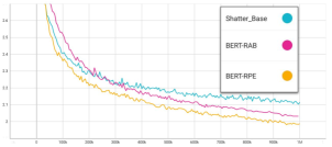
Figure 4: MLM valid loss for base-size models.

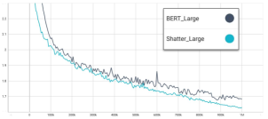
Figure 5: MLM valid loss for large-size models.

Instead of the word-piece tokenizer (Wu et al., 2016) used in BERT, we use sentence-piece (Kudo and Richardson, 2018) for tokenization, on account of its easy usage and fast speed. The pretraining corpus is lower-cased and the vocabulary size set to 32k. This same tokenizer is used in all models in our experiments, for fair comparison.

To save pretraining time, we tokenize the corpus in advance and cache the results to files. The tokenization can be done with 20 parallel 4-core CPU machines in 2 hours. Following RoBERTa (Liu et al., 2019), we use Masked Language Modeling (MLM) as the pretraining objective, without Next Sentence Prediction.

For optimization we use Adam with $0.01$ weight decay (Bentivogli et al., 2009). The learning rate is set to 1e-4, with 10k steps warmup then linear decay to 0.

For validation we use the Penn Tree Bank corpus (Marcus et al., 1994), and the valid loss is plotted in Figure 1 (for our model variants and BERT_Base), Figure 4 (for base-size models) and Figure 5 (for large-size models). In Figure 4, BERT-RPE consistently outperforms other models, while Shatter_Base shows faster convergence than BERT-RAB, which roughly aligns with the convergence of finetuned performance (Figure 3). In Figure 5, Shatter_Large outperforms BERT_Large. The valid loss for XLNet is not shown in the figures, since XLNet is pretrained with PLM instead of MLM.

A.3 Ablation on GLUE

In Table 6, we compare the finetuned performance of our model variants developed in §3. Mostly, the performance of Shatter_Base $\geq$ Part_Bias $>$ 1H_Sigmoid $>$ Part_Mask, which aligns with the comparison of pretraining loss in Figure 1. The performance of Shatter_Base and Part_Bias are close, but Shatter_Base slightly outperforms Part_Bias on MNLI and QQP.

A.4 Sequence Classification Strategy

We further compare different sequence classification strategies in Table 7. The sequence classification method originally used in BERT (Devlin et al., 2019), which takes the hidden state at the [CLS] token, is indicated by a “[CLS]” suffix in the table. It is compared with our modified sequence classification method described in §3.4.

For BERT_Base, the difference in sequence classification strategy does not affect finetuned performance; but for Shatter_Base and BERT-RPE, our modified method is generally better, which suggests that our method can better cope with the relative position modeling of the [CLS] token.

References

- Ba et al. (2016) Jimmy Lei Ba, Jamie Ryan Kiros, and Geoffrey E. Hinton. 2016. Layer normalization.
- Beltagy et al. (2020) Iz Beltagy, Matthew E. Peters, and Arman Cohan. 2020. Longformer: The long-document transformer. CoRR, abs/2004.05150.
- Bentivogli et al. (2009) Luisa Bentivogli, Peter Clark, Ido Dagan, and Danilo Giampiccolo. 2009. The fifth pascal recognizing textual entailment challenge. In TAC.
- Cer et al. (2017) Daniel Cer, Mona Diab, Eneko Agirre, Inigo Lopez-Gazpio, and Lucia Specia. 2017. Semeval-2017 task 1: Semantic textual similarity-multilingual and cross-lingual focused evaluation. arXiv preprint arXiv:1708.00055.
- Chen et al. (2021) Pu-Chin Chen, Henry Tsai, Srinadh Bhojanapalli, Hyung Won Chung, Yin-Wen Chang, and Chun-Sung Ferng. 2021. Demystifying the better performance of position encoding variants for transformer. CoRR, abs/2104.08698.
- Chen et al. (2020) Xiaohan Chen, Yu Cheng, Shuohang Wang, Zhe Gan, Zhangyang Wang, and Jingjing Liu. 2020. Earlybert: Efficient bert training via early-bird lottery tickets. arXiv preprint arXiv:2101.00063.
- Cheng et al. (2016) Jianpeng Cheng, Li Dong, and Mirella Lapata. 2016. Long short-term memory-networks for machine reading. In Proceedings of the 2016 Conference on Empirical Methods in Natural Language Processing, pages 551–561, Austin, Texas. Association for Computational Linguistics.
- Child et al. (2019) Rewon Child, Scott Gray, Alec Radford, and Ilya Sutskever. 2019. Generating long sequences with sparse transformers. CoRR, abs/1904.10509.
- Choromanski et al. (2020) Krzysztof Choromanski, Valerii Likhosherstov, David Dohan, Xingyou Song, Andreea Gane, Tamás Sarlós, Peter Hawkins, Jared Davis, Afroz Mohiuddin, Lukasz Kaiser, David Belanger, Lucy J. Colwell, and Adrian Weller. 2020. Rethinking attention with performers. CoRR, abs/2009.14794.
- Clark et al. (2019) Christopher Clark, Kenton Lee, Ming-Wei Chang, Tom Kwiatkowski, Michael Collins, and Kristina Toutanova. 2019. Boolq: Exploring the surprising difficulty of natural yes/no questions. arXiv preprint arXiv:1905.10044.
- Clark et al. (2020) Kevin Clark, Minh-Thang Luong, Quoc V Le, and Christopher D Manning. 2020. Electra: Pre-training text encoders as discriminators rather than generators. arXiv preprint arXiv:2003.10555.
- Devlin et al. (2019) Jacob Devlin, Ming-Wei Chang, Kenton Lee, and Kristina Toutanova. 2019. BERT: Pre-training of deep bidirectional transformers for language understanding. In Proceedings of the 2019 Conference of the North American Chapter of the Association for Computational Linguistics: Human Language Technologies, Volume 1 (Long and Short Papers), pages 4171–4186, Minneapolis, Minnesota. Association for Computational Linguistics.
- Dolan and Brockett (2005) William B Dolan and Chris Brockett. 2005. Automatically constructing a corpus of sentential paraphrases. In Proceedings of the Third International Workshop on Paraphrasing (IWP2005).
- He et al. (2020) Pengcheng He, Xiaodong Liu, Jianfeng Gao, and Weizhu Chen. 2020. Deberta: Decoding-enhanced bert with disentangled attention. arXiv preprint arXiv:2006.03654.
- Jiang et al. (2020) Zihang Jiang, Weihao Yu, Daquan Zhou, Yunpeng Chen, Jiashi Feng, and Shuicheng Yan. 2020. Convbert: Improving BERT with span-based dynamic convolution. CoRR, abs/2008.02496.
- Ke et al. (2020) Guolin Ke, Di He, and Tie-Yan Liu. 2020. Rethinking positional encoding in language pre-training. arXiv preprint arXiv:2006.15595.
- Khashabi et al. (2018) Daniel Khashabi, Snigdha Chaturvedi, Michael Roth, Shyam Upadhyay, and Dan Roth. 2018. Looking beyond the surface: A challenge set for reading comprehension over multiple sentences. In Proceedings of the 2018 Conference of the North American Chapter of the Association for Computational Linguistics: Human Language Technologies, Volume 1 (Long Papers), pages 252–262.
- Kingma and Ba (2014) Diederik P Kingma and Jimmy Ba. 2014. Adam: A method for stochastic optimization. arXiv preprint arXiv:1412.6980.
- Kitaev et al. (2020) Nikita Kitaev, Lukasz Kaiser, and Anselm Levskaya. 2020. Reformer: The efficient transformer. CoRR, abs/2001.04451.
- Kudo and Richardson (2018) Taku Kudo and John Richardson. 2018. Sentencepiece: A simple and language independent subword tokenizer and detokenizer for neural text processing. arXiv preprint arXiv:1808.06226.
- Lan et al. (2019) Zhenzhong Lan, Mingda Chen, Sebastian Goodman, Kevin Gimpel, Piyush Sharma, and Radu Soricut. 2019. ALBERT: A lite BERT for self-supervised learning of language representations. CoRR, abs/1909.11942.
- Lee-Thorp et al. (2021) James Lee-Thorp, Joshua Ainslie, Ilya Eckstein, and Santiago Ontañón. 2021. Fnet: Mixing tokens with fourier transforms. CoRR, abs/2105.03824.
- Liu et al. (2019) Yinhan Liu, Myle Ott, Naman Goyal, Jingfei Du, Mandar Joshi, Danqi Chen, Omer Levy, Mike Lewis, Luke Zettlemoyer, and Veselin Stoyanov. 2019. Roberta: A robustly optimized bert pretraining approach. arXiv preprint arXiv:1907.11692.
- Marcus et al. (1994) Mitchell Marcus, Grace Kim, Mary Ann Marcinkiewicz, Robert MacIntyre, Ann Bies, Mark Ferguson, Karen Katz, and Britta Schasberger. 1994. The Penn Treebank: Annotating predicate argument structure. In Human Language Technology: Proceedings of a Workshop held at Plainsboro, New Jersey, March 8-11, 1994.
- Michel et al. (2019) Paul Michel, Omer Levy, and Graham Neubig. 2019. Are sixteen heads really better than one? arXiv preprint arXiv:1905.10650.
- Parikh et al. (2016) Ankur Parikh, Oscar Täckström, Dipanjan Das, and Jakob Uszkoreit. 2016. A decomposable attention model for natural language inference. In Proceedings of the 2016 Conference on Empirical Methods in Natural Language Processing, pages 2249–2255, Austin, Texas. Association for Computational Linguistics.
- Raffel et al. (2019) Colin Raffel, Noam Shazeer, Adam Roberts, Katherine Lee, Sharan Narang, Michael Matena, Yanqi Zhou, Wei Li, and Peter J. Liu. 2019. Exploring the limits of transfer learning with a unified text-to-text transformer. CoRR, abs/1910.10683.
- Rajpurkar et al. (2016) Pranav Rajpurkar, Jian Zhang, Konstantin Lopyrev, and Percy Liang. 2016. Squad: 100,000+ questions for machine comprehension of text. arXiv preprint arXiv:1606.05250.
- Sellam et al. (2021) Thibault Sellam, Steve Yadlowsky, Jason Wei, Naomi Saphra, Alexander D’Amour, Tal Linzen, Jasmijn Bastings, Iulia Turc, Jacob Eisenstein, Dipanjan Das, et al. 2021. The multiberts: Bert reproductions for robustness analysis. arXiv preprint arXiv:2106.16163.
- Shaw et al. (2018) Peter Shaw, Jakob Uszkoreit, and Ashish Vaswani. 2018. Self-attention with relative position representations. arXiv preprint arXiv:1803.02155.
- Socher et al. (2013) Richard Socher, Alex Perelygin, Jean Wu, Jason Chuang, Christopher D. Manning, Andrew Ng, and Christopher Potts. 2013. Recursive deep models for semantic compositionality over a sentiment treebank. In Proceedings of the 2013 Conference on Empirical Methods in Natural Language Processing, pages 1631–1642, Seattle, Washington, USA. Association for Computational Linguistics.
- Vaswani et al. (2017) Ashish Vaswani, Noam Shazeer, Niki Parmar, Jakob Uszkoreit, Llion Jones, Aidan N Gomez, Łukasz Kaiser, and Illia Polosukhin. 2017. Attention is all you need. In Advances in neural information processing systems, pages 5998–6008.
- Voita et al. (2019) Elena Voita, David Talbot, Fedor Moiseev, Rico Sennrich, and Ivan Titov. 2019. Analyzing multi-head self-attention: Specialized heads do the heavy lifting, the rest can be pruned. arXiv preprint arXiv:1905.09418.
- Wang et al. (2019) Alex Wang, Yada Pruksachatkun, Nikita Nangia, Amanpreet Singh, Julian Michael, Felix Hill, Omer Levy, and Samuel R Bowman. 2019. Superglue: A stickier benchmark for general-purpose language understanding systems. arXiv preprint arXiv:1905.00537.
- Wang et al. (2018) Alex Wang, Amanpreet Singh, Julian Michael, Felix Hill, Omer Levy, and Samuel R Bowman. 2018. Glue: A multi-task benchmark and analysis platform for natural language understanding. arXiv preprint arXiv:1804.07461.
- Warstadt et al. (2019) Alex Warstadt, Amanpreet Singh, and Samuel R. Bowman. 2019. Neural network acceptability judgments. Transactions of the Association for Computational Linguistics, 7:625–641.
- Wennberg and Henter (2021) Ulme Wennberg and Gustav Eje Henter. 2021. The case for translation-invariant self-attention in transformer-based language models. arXiv preprint arXiv:2106.01950.
- Williams et al. (2018) Adina Williams, Nikita Nangia, and Samuel Bowman. 2018. A broad-coverage challenge corpus for sentence understanding through inference. In Proceedings of the 2018 Conference of the North American Chapter of the Association for Computational Linguistics: Human Language Technologies, Volume 1 (Long Papers), pages 1112–1122, New Orleans, Louisiana. Association for Computational Linguistics.
- Wolf et al. (2020) Thomas Wolf, Lysandre Debut, Victor Sanh, Julien Chaumond, Clement Delangue, Anthony Moi, Pierric Cistac, Tim Rault, Remi Louf, Morgan Funtowicz, Joe Davison, Sam Shleifer, Patrick von Platen, Clara Ma, Yacine Jernite, Julien Plu, Canwen Xu, Teven Le Scao, Sylvain Gugger, Mariama Drame, Quentin Lhoest, and Alexander Rush. 2020. Transformers: State-of-the-art natural language processing. In Proceedings of the 2020 Conference on Empirical Methods in Natural Language Processing: System Demonstrations, pages 38–45, Online. Association for Computational Linguistics.
- Wu et al. (2016) Yonghui Wu, Mike Schuster, Zhifeng Chen, Quoc V Le, Mohammad Norouzi, Wolfgang Macherey, Maxim Krikun, Yuan Cao, Qin Gao, Klaus Macherey, et al. 2016. Google’s neural machine translation system: Bridging the gap between human and machine translation. arXiv preprint arXiv:1609.08144.
- Yang et al. (2019) Zhilin Yang, Zihang Dai, Yiming Yang, Jaime Carbonell, Russ R Salakhutdinov, and Quoc V Le. 2019. Xlnet: Generalized autoregressive pretraining for language understanding. Advances in neural information processing systems, 32.
- Zhu et al. (2015) Yukun Zhu, Ryan Kiros, Rich Zemel, Ruslan Salakhutdinov, Raquel Urtasun, Antonio Torralba, and Sanja Fidler. 2015. Aligning books and movies: Towards story-like visual explanations by watching movies and reading books. In Proceedings of the IEEE international conference on computer vision, pages 19–27.