Logarithmic Schrödinger equation and isothermal fluids

Abstract.

We consider the large time behavior in two types of equations, posed on the whole space ${\mathbb{R}}^{d}$: the Schrödinger equation with a logarithmic nonlinearity on the one hand; compressible, isothermal, Euler, Korteweg and quantum Navier-Stokes equations on the other hand. We explain some connections between the two families of equations, and show how these connections may help having an insight in all cases. We insist on some specific aspects only, and refer to the cited articles for more details, and more complete statements. We try to give a general picture of the results, and present some heuristical arguments that can help the intuition, which are not necessarily found in the mentioned articles.

1. Introduction

1.1. Linear equations

As a preliminary, and for future comparison with the logarithmic Schrödinger equation, we recall some basic facts regarding the large time dynamics for the linear heat equation and the linear Schrödinger equation, on ${\mathbb{R}}^{d}$.

1.1.1. Heat equation

Consider the Cauchy problem

$${\partial}_{t}u=\frac{1}{2}\Delta u,\quad x\in{\mathbb{R}}^{d},\quad u_{\mid t=0}=u_{0}\in L^{1}({\mathbb{R}}^{d}).$$

The solution is given by the explicit formula: $\displaystyle u(t,x)=\frac{1}{(2\pi t)^{d/2}}\int_{{\mathbb{R}}^{d}}e^{-\frac{|x-y|^{2}}{2t}}u_{0}(y)dy.$ This formula is classical, and follows from Fourier analysis, see e.g. [70]. To fix ideas, we normalize the Fourier transform as

$$\hat{f}(\xi)=\frac{1}{(2\pi)^{d/2}}\int_{{\mathbb{R}}^{d}}e^{-ix\cdot\xi}f(x)dx,\quad f\in{\mathcal{S}}({\mathbb{R}}^{d}).$$

The Fourier transform of $u$ at time $t$ is given by

$$\hat{u}(t,\xi)=e^{-\frac{t}{2}|\xi|^{2}}\hat{u}_{0}(\xi)=\underbrace{e^{-\frac{t}{2}|\xi|^{2}}\hat{u}_{0}(0)}_{\text{order }t^{-d/(2p)}\text{ in }L^{p}}+\underbrace{e^{-\frac{t}{2}|\xi|^{2}}\left(\hat{u}_{0}(\xi)-\hat{u}_{0}(0)\right)}_{\mathcal{O}\left(|\xi|e^{-\frac{t}{2}|\xi|^{2}}\right):\text{ order }t^{-(d+1)/(2p)}\text{ in }L^{p}}.$$

If $m:=\int_{{\mathbb{R}}^{d}}u_{0}=(2\pi)^{d/2}\hat{u}_{0}(0)\not=0$, we infer, by the Fourier inverse formula,

$$u(t,x)\mathop{\sim}\limits_{t\rightarrow\infty}\frac{m}{(2\pi t)^{d/2}}e^{-|x|^{2}/(2t)},$$

and we leave out the discussion on the norms involved above: the key message is that the large time description involves a universal diffusive rate, and a universal Gaussian profile, the initial data appears only through its mass $m$.

1.1.2. Schrödinger equation

For the Schrödinger equation, the initial datum naturally belongs to $L^{2}$,

$$i{\partial}_{t}u+\frac{1}{2}\Delta u=0,\quad x\in{\mathbb{R}}^{d},\quad u_{\mid t=0}=u_{0}\in L^{2}({\mathbb{R}}^{d}).$$

Again, the solution is given explicitly, now by an oscillatory integral:

$$u(t,x)=\frac{1}{(2i\pi t)^{d/2}}\int_{{\mathbb{R}}^{d}}e^{i\frac{|x-y|^{2}}{2t}}u_{0}(y)dy.$$

We emphasize two consequences:

• Dispersion: $\displaystyle\|u(t)\|_{L^{\infty}({\mathbb{R}}^{d})}\lesssim\frac{1}{|t|^{d/2}}\|u_{0}\|_{L^{1}({\mathbb{R}}^{d})}.$

• Large time description: $\left\lVert u(t)-A(t)u_{0}\right\rVert_{L^{2}({\mathbb{R}}^{d})}\mathop{\longrightarrow}\limits_{t\rightarrow\pm\infty}0$, where

  $$A(t)u_{0}(x)=\frac{1}{(it)^{d/2}}\hat{u}_{0}\left(\frac{x}{t}\right)e^{i\frac{\lvert x\rvert^{2}}{2t}}.$$

  We now have a universal oscillation, but the profile depends on the initial data, through its Fourier transform.

To check the second point, expanding the argument of the exponential in the oscillatory integral, we can write

$$u(t,x)=M_{t}D_{t}\mathcal{F}M_{t}u_{0}(x),$$

where $\mathcal{F}$ stands for the Fourier transform, $M_{t}$ is the multiplication by $e^{i|x|^{2}/(2t)}$, and $D_{t}$ is the time dependent dilation

$$D_{t}\varphi(x)=\frac{1}{(it)^{d/2}}\varphi\left(\frac{x}{t}\right).$$

Then $A(t)u_{0}=M_{t}D_{t}\mathcal{F}u_{0}$, and the approximation follows from the limit $M_{t}\to 1$ in $L^{2}$, as $t\to\infty$, as granted by the dominated convergence theorem.

Example 1.1 (Explicit computation in the Gaussian case).

The evolution of Gaussian initial data is given, for $z\in{\mathbb{C}}$ such that $\operatorname{Re}z>0$, by:

$$e^{i\frac{t}{2}\Delta}\left(e^{-z\frac{|x|^{2}}{2}}\right)=\frac{1}{(1+itz)^{d/2}}e^{-\frac{z}{1+itz}\frac{|x|^{2}}{2}}.$$

1.2. Nonlinear Schrödinger equation: the usual nonlinearity

We recall a few standard properties related to the nonlinear Schrödinger equation with power-like nonlinearity. These properties can be found e.g. in [33]. For $\lambda\in{\mathbb{R}}$, and $0<{\sigma}<\frac{2}{(d-2)_{+}}$, consider:

(1.1) $$i{\partial}_{t}u+\frac{1}{2}\Delta u=\lambda|u|^{2{\sigma}}u,\quad x\in{\mathbb{R}}^{d},\quad u_{\mid t=0}=u_{0}\in H^{1}({\mathbb{R}}^{d}).$$

Under our assumption on ${\sigma}$, the nonlinearity is $H^{1}$-subcritical (the $L^{2{\sigma}+2}$-norm in the energy below is controlled by the $H^{1}$-norm, thanks to Sobolev embedding), and the Cauchy problem (1.1) is locally well-posed in $H^{1}({\mathbb{R}}^{d})$. The standard proof relies on Strichartz estimates, and a fixed point argument on Duhamel’s formula; the nonlinearity is thus considered as a perturbation, the problem is semilinear. The situation is completely different in the case of equations from (compressible) fluid mechanics, addressed in the second part of this survey.

1.2.1. Invariants

Equation 1.1 is invariant under space and time translation, as well as under the gauge transforms

$$u(t,x)\mapsto e^{i\theta}u(t,x),\quad\theta\in{\mathbb{R}}.$$

The Galilean invariance reads as follows: if $u(t,x)$ solves (1.1), then for any ${\mathbf{v}}\in{\mathbb{R}}^{d}$, so does

(1.2) $$u(t,x-{\mathbf{v}}t)e^{i{\mathbf{v}}\cdot x-i|{\mathbf{v}}|^{2}t/2}.$$

(With a different initial datum.) This property is useful to construct multisolitons (with different velocities), as in e.g. [68].
The following quantities are formally independent of time:

Mass: $$M(u(t)):=\|u(t)\|_{L^{2}({\mathbb{R}}^{d})}^{2},$$

Momentum: $$J(u(t)):=\operatorname{Im}\int_{{\mathbb{R}}^{d}}\bar{u}(t,x)\nabla u(t,x)dx,$$

Energy: $$E(u(t)):=\frac{1}{2}\|\nabla u(t)\|_{L^{2}({\mathbb{R}}^{d})}^{2}+\frac{\lambda}{{\sigma}+1}\|u(t)\|_{L^{2{\sigma}+2}({\mathbb{R}}^{d})}^{2{\sigma}+2}.$$

According to the sign of $\lambda$, the energy is or is not a positive functional.

1.2.2. Defocusing case

If $\lambda>0$: the local well-posedness in $H^{1}$ and the conservations of mass and energy imply global existence ($u\in L^{\infty}({\mathbb{R}};H^{1}({\mathbb{R}}^{d}))$), and if ${\sigma}>2/d$, the solution behaves asymptotically like a linear solution,

(1.3) $$\exists u_{+}\in H^{1}({\mathbb{R}}^{d}),\quad\|u(t)-e^{i\frac{t}{2}\Delta}u_{+}\|_{H^{1}({\mathbb{R}}^{d})}\mathop{\longrightarrow}\limits_{t\rightarrow\infty}0.$$

The (inverse of) the wave operator is not trivial: $u_{0}\mapsto u_{+}$ is one-to-one. In view of the description in the linear case, this means that the large time asymptotics involves a universal oscillation, a universal dispersion, and a somehow arbitrary profile.

If we assume in addition that $x\mapsto|x|u_{0}(x)$ belongs to $L^{2}({\mathbb{R}}^{d})$, then the same conclusion as above is known to remain valid for some smaller values of ${\sigma}$, but not too small. Typically, for ${\sigma}\leqslant 1/d$, if $u$ solves (1.1), then its large time behavior cannot be directly compared to the linear evolution, in the sense that if there exists $u_{+}\in L^{2}({\mathbb{R}}^{d})$ such that

$$\|u(t)-e^{i\frac{t}{2}\Delta}u_{+}\|_{L^{2}({\mathbb{R}}^{d})}\mathop{\longrightarrow}\limits_{t\rightarrow\infty}0,$$

then necessarily $u_{0}=u_{+}=0$ (hence $u\equiv 0$), from [13]. This is due to the presence of long range effects, and scattering theory must be modified, see e.g. [58] and references therein. We will give reasons to consider that the limit ${\sigma}\to 0$ leads to the logarithmic Schrödinger equation (see Section 7), and show that the dynamical properties related to that model are very specific.

1.2.3. Focusing case

If $\lambda<0$, finite time blow-up is possible when ${\sigma}\geqslant 2/d$, as proved typically by a virial computation (the second order derivative of the function $t\mapsto\|xu(t)\|_{L^{2}({\mathbb{R}}^{d})}^{2}$ may be smaller than a negative constant, [48], see also [33]), and blow-up is characterized by the existence of a finite $T^{*}$ such that

$$\lim_{t\to T^{*}}\|\nabla u(t)\|_{L^{2}}=\infty.$$

For ${\sigma}\geqslant 2/d$, small initial data generate global solutions, which are moreover asymptotically linear in the sense of (1.3).

Finally, we evoke the existence of large standing waves, of the form $u(t,x)=e^{i\omega t}\psi(x)$. When $\psi$ is a ground state (which is unique up to the invariants of the associated elliptic equation), the above standing wave is orbitally stable if and only if ${\sigma}<2/d$ (instability by blow-up occurs when ${\sigma}\geqslant 2/d$, [15, 80]: small – in $H^{1}$ – perturbations of the standing wave may generate a solution which blows up in finite time). The right notion is indeed orbital stability, as opposed to asymptotic stability of the standing wave, due to the invariants of the equation: in view of the Galilean invariance (1.2), a small initial perturbation $\psi(x)e^{i\mathbf{v}\cdot x}$ ($|\mathbf{v}|\ll 1$) will generate a standing wave whose “support” becomes distinct from the support of $u$ for sufficiently large time. Orbital stability consists in taking the invariants of the equation into account: in the present case, this means that for any $\varepsilon>0$, there exists $\eta>0$ such that if

$$\text{if}\quad\|\tilde{u}_{0}-\psi\|_{H^{1}}\leqslant\eta,\quad\text{then}\quad\sup_{t\in{\mathbb{R}}}\inf_{\theta\in{\mathbb{R}}}\inf_{y\in{\mathbb{R}}^{d}}\|\tilde{u}(t)-e^{i\theta}\phi(\cdot-y)\|_{H^{1}}\leqslant\varepsilon,$$

where $\tilde{u}$ is the solution to (1.1) with initial data $\tilde{u}_{0}$. See e.g. [33].

We will see that there are many differences in the case where the power-like nonlinearity is replaced by a logarithmic nonlinearity.

1.3. Logarithmic Schrödinger equation

We now consider the Cauchy problem

(1.4) $$i{\partial}_{t}u+\frac{1}{2}\Delta u=\lambda\ln\left(|u|^{2}\right)u,\quad u_{\mid t=0}=u_{0},$$

with $x\in{\mathbb{R}}^{d}$, $d\geqslant 1$, and $\lambda\in{\mathbb{R}}$. This model was introduced in [16] to satisfy the following tensorization property: if the initial datum is a tensor product,

$$u_{0}(x)=\prod_{j=1}^{d}u_{0j}(x_{j}),$$

then the solution to (1.4) is given by

$$u(t,x)=\prod_{j=1}^{d}u_{j}(t,x_{j}),$$

where each $u_{j}$ solves a one-dimensional equation,

$$i{\partial}_{t}u_{j}+\frac{1}{2}{\partial}_{x_{j}}^{2}u_{j}=\lambda\ln\left(|u_{j}|^{2}\right)u_{j},\quad u_{j\mid t=0}=u_{0j}.$$

The logarithmic nonlinearity turns out to be the only one satisfying such a property. This nonlinearity has then been proposed to model various physical phenomena, e.g. quantum optics [25, 63], nuclear physics [59], transport and diffusion phenomena [69, 56], open quantum systems [81, 61], effective quantum gravity [82], theory of superfluidity and Bose-Einstein condensation [11]. This tensorization property is classical when the linear Schrödinger equation is considered, and might suggest that nonlinear effects in (1.4) are weak: we will see that on the contrary, the dynamical properties associated to (1.4) are rather unique. This is due to the singularity of the logarithm at the origin.

Like above, (1.4) is invariant under space and time translations, gauge and Galilean transforms. We still have conservation of mass, momentum and energy, but the expression of the latter has changed:

$$M(u(t))=\|u(t)\|_{L^{2}({\mathbb{R}}^{d})}^{2},$$

$$J(u(t))=\operatorname{Im}\int_{{\mathbb{R}}^{d}}\bar{u}(t,x)\nabla u(t,x)dx,$$

$$E(u(t))=\frac{1}{2}\|\nabla u(t)\|_{L^{2}({\mathbb{R}}^{d})}^{2}+\lambda\int_{{\mathbb{R}}^{d}}|u(t,x)|^{2}\left(\ln|u(t,x)|^{2}-1\right)dx.$$

In view of the conservation of mass, we rather consider the energy

(1.5) $$E(u(t)):=\frac{1}{2}\|\nabla u(t)\|_{L^{2}({\mathbb{R}}^{d})}^{2}+\lambda\int_{{\mathbb{R}}^{d}}|u(t,x)|^{2}\ln|u(t,x)|^{2}dx.$$

The energy has no definite sign, and it is not completely clear to decide about the influence of the sign of $\lambda$ on the dynamics. However, a formal argument suggests that when $\lambda<0$, solutions cannot disperse: indeed, if $u$ is dispersive, then it morally goes to zero pointwise, and the argument of the logarithm in the energy going to zero, the factor of $\lambda$ goes to $-\infty$: if $\lambda<0$, this contradicts the conservation of the energy, which would then become infinite. On the other hand, if $\lambda>0$, this argument shows that if a solution is dispersive, then its $\dot{H}^{1}$-norm becomes infinite in the large time régime.

Another unusual feature of (1.4) concerns the effect of the size of the initial data on the dynamics: If $u$ solves (1.4), then for all $k\in{\mathbb{C}}$, so does

(1.6) $$u_{k}(t,x):=ku(t,x)e^{-it\lambda\ln|k|^{2}}.$$

This shows that the size of the initial data alters the dynamics only through a purely time dependent oscillation, a feature which is fairly unusual for a nonlinear equation. For $k>0$, we readily compute

$$\frac{d}{dk}u_{k}(t,x)=(1-2it)u(t,x)e^{-it\lambda\ln|k|^{2}}.$$

The above quantity has no limit as $k\to 0$ for $t>0$: the flow map $u_{0}\mapsto u(t)$ cannot be $C^{1}$, whichever function spaces are considered for $u_{0}$ and $u(t)$, respectively; it is at most Lipschitzean.

The next few sections are dedicated to the analysis of the logarithmic Schrödinger equation (1.4). In Section 5, we will see a first connection with models from compressible fluid mechanics, and from Section 6 to the end of the survey, we will focus our attention on such models and some of their generalizations.

1.4. Schematic summary: power vs. logarithmic nonlinearity

In the following tables, we give an overview of the results presented below, in order to emphasize some differences due to the nature of the nonlinearity. To avoid unnecessary technical details, we assume in all cases that the initial datum $u_{0}$ belongs to $\Sigma$, defined by

$$\Sigma=H^{1}\cap\mathcal{F}(H^{1})=\{f\in H^{1}({\mathbb{R}}^{d}),\ x\mapsto|x|f(x)\in L^{2}({\mathbb{R}}^{d})\},$$

that the nonlinearity is $H^{1}$-subcritical, $0<{\sigma}<\frac{2}{(d-2)_{+}}$, and do not try to invoke sharp results. (GWP stands for global well-posedness.)

Case $\lambda>0.$

Equation	(1.1)	(1.4)
Nonlinearity	$\lambda|u|^{2{\sigma}}u$	$\lambda\ln(|u|^{2})u$
GWP in $H^{1}$	Yes	Yes
Dispersion: $(\delta(t))^{-d/2}$	$\delta(t)=t$ (at least if $\sigma\geqslant 2/d$)	$\delta(t)=2t\sqrt{\lambda\ln t}$
$\displaystyle\lim_{t\to\infty}(\delta(t))^{d/2}|u(t,x\delta(t))|$	$|v_{+}|$ for any $v_{+}\in\Sigma$ (if ${\sigma}\geqslant 2/d$)	$\displaystyle\frac{\|u_{0}\|_{L^{2}}}{\pi^{d/4}}e^{-|x|^{2}/2}$
Growth of $H^{1}$ norm	Never	Always

In connection with the results recalled in Sections 1.1.2 and 1.2, $v_{+}=\hat{u}_{+}$, the Fourier transform of the asymptotic state $u_{+}$, which may be any function in $\Sigma$.

Case $\lambda<0.$

Equation	(1.1)	(1.4)
Nonlinearity	$\lambda|u|^{2{\sigma}}u$	$\lambda\ln(|u|^{2})u$
GWP in $H^{1}$	For sure, if ${\sigma}<2/d$	Yes
Finite time blow up	Possible if ${\sigma}\geqslant 2/d$	Never
Dispersion	For small data, if ${\sigma}\geqslant 2/d$	Never
Standing waves	Exist	Exist
Ground states are orbitally stable	Yes, iff ${\sigma}<2/d$	Yes
Breathers	?	Exist
Multisolitons	Exist	Exist
Multibreathers	?	Exist

2. Cauchy problem

In view of the expression (1.5), the natural energy space is given by

$$W:=\Big{\{}u\in H^{1}({\mathbb{R}}^{d})\,,\,x\mapsto|u(x)|^{2}\ln|u(x)|^{2}\in L^{1}({\mathbb{R}}^{d})\Big{\}}\,.$$

The Cauchy problem (1.4) is indeed solved in $W$, provided that $\lambda<0$:

Theorem 2.1 ([34]).

Suppose $\lambda<0$ and $u_{0}\in W$: there exists a unique, global solution $u\in C({\mathbb{R}};W)$ to (1.4). The mass $M(u)$ and the energy $E(u)$ are independent of time.

The proof given in [34] relies on compactness arguments, using a regularization of the nonlinearity. An alternative proof has been proposed more recently by Masayuki Hayashi [57], providing the strong convergence of a sequence of approximate solutions. See also [52] for the local Cauchy problem in $H^{2}$ on bounded 3D domains. We emphasize that the sign of $\lambda$ appears when seeking a priori estimates: if $\lambda<0$, we have

$$0\leqslant E_{+}(u(t)) :=\frac{1}{2}\|\nabla u(t)\|_{L^{2}({\mathbb{R}}^{d})}^{2}+\lambda\int_{|u|<1}|u(t,x)|^{2}\ln|u(t,x)|^{2}dx$$

$$\leqslant E(u_{0})\underbrace{-\lambda}_{+|\lambda|}\int_{|u|>1}|u(t,x)|^{2}\ln|u(t,x)|^{2}dx.$$

Since the logarithm grows slowly,

$$\int_{|u|>1}|u(t,x)|^{2}\ln|u(t,x)|^{2}dx \leqslant C_{\varepsilon}\int_{|u|>1}|u(t,x)|^{2+\varepsilon}dx$$

$$\lesssim\|u(t)\|_{L^{2}({\mathbb{R}}^{d})}^{2+\varepsilon-\varepsilon d/2}\|\nabla u(t)\|_{L^{2}({\mathbb{R}}^{d})}^{\varepsilon d/2},$$

where we have used Gagliardo-Nirenberg inequalities, for $\varepsilon<2d/(d-2)_{+}$. Using the conservation of mass, this implies

$$E_{+}(u(t))\leqslant E(u_{0})+C_{\varepsilon}E_{+}\left(u(t)\right)^{\varepsilon d/4}.$$

Therefore, picking $\varepsilon>0$ sufficiently small yields $E_{+}\in L^{\infty}({\mathbb{R}})$, hence (resuming the above inequality) $u\in L^{\infty}({\mathbb{R}};W)$.

Remark 2.2.

In the case $\lambda>0$, the same strategy would require the control of

$$\int_{|u|<1}|u(t,x)|^{2}\ln\frac{1}{|u(t,x)|^{2}}dx\leqslant C_{\varepsilon}\int_{|u|<1}|u(t,x)|^{2-\varepsilon}dx.$$

The above Lebesgue norm involves an index below $2$, and Sobolev embedding cannot help: we will see that the finiteness of a momentum in $L^{2}$ saves the day.

Uniqueness follows from the algebraic property discovered in [34]:

Lemma 2.3 ([34]).

We have

$$\left|\operatorname{Im}\left(\left(z_{2}\ln|z_{2}|^{2}-z_{1}\ln|z_{1}|^{2}\right)\left(\bar{z}_{2}-\bar{z}_{1}\right)\right)\right|\leqslant 4|z_{2}-z_{1}|^{2}\,,\quad\forall z_{1},z_{2}\in{\mathbb{C}}\,.$$

Formally, if $u_{1}$ and $u_{2}$ are two solutions of (1.4), $w:=u_{2}-u_{1}$ solves

$$i{\partial}_{t}w+\frac{1}{2}\Delta w=\lambda\left(u_{2}\ln|u_{2}|^{2}-u_{1}\ln|u_{1}|^{2}\right).$$

Multiplying the above equation by $\bar{w}$, integrating in space and considering the imaginary part, Lemma 2.3 yields

$$\frac{1}{2}\frac{d}{dt}\|w(t)\|_{L^{2}}^{2}\leqslant 4|\lambda|\|w(t)\|_{L^{2}}^{2},$$

and Gronwall lemma provides uniqueness. One has to be cautious though, this argument is fully justified provided that we know $u\in C({\mathbb{R}};L^{2})$, a property which is satisfied for $u\in L^{\infty}({\mathbb{R}};W)$, as shown by a careful examination of (1.4); see [34] for details.

This strategy was adapted in [51] to consider the case $\lambda>0$, under the extra assumption $|x|^{1/2}u_{0}\in L^{2}({\mathbb{R}}^{d})$, for $d=3$.

In [31], another compactness method was proposed, consisting in neutralizing the singularity of the logarithm at the origin: for $\varepsilon>0$, consider $u^{\varepsilon}$ solution to

(2.1) $$i{\partial}_{t}u^{\varepsilon}+\frac{1}{2}\Delta u^{\varepsilon}=\lambda\ln\left(\varepsilon+|u^{\varepsilon}|^{2}\right)u^{\varepsilon},\quad u^{\varepsilon}_{\mid t=0}=u_{0}.$$

For fixed $\varepsilon>0$, the above nonlinearity is smooth and $L^{2}$-subcritical, and there exists a unique solution at the $L^{2}$-level [75]. Assuming $u_{0}\in H^{1}$, $|x|^{\alpha}u_{0}\in L^{2}$ for some $0<\alpha\leqslant 1$, we can prove a priori estimates on bounded time intervals, which are uniform in $\varepsilon\in]0,1]$, and infer:

Theorem 2.4 ([31]).

Let $\lambda\in{\mathbb{R}}$, $u_{0}\in H^{1}\cap\mathcal{F}(H^{\alpha})$ for some $0<\alpha\leqslant 1$: (1.4) has a unique, global solution $u\in L^{\infty}_{\rm loc}({\mathbb{R}};H^{1}\cap\mathcal{F}(H^{\alpha}))$. The mass $M(u)$ and the energy $E(u)$ are independent of time.

Heuristically, the assumption $|x|^{\alpha}u_{0}\in L^{2}$ for some $0<\alpha\leqslant 1$ seems rather natural in view of Remark 2.2. Indeed, considering $0<\eta<\frac{4\alpha}{d+2\alpha}$, we have

(2.2) $$\int_{{\mathbb{R}}^{d}}|u|^{2-\eta}\lesssim\|u\|_{L^{2}}^{2-\eta-\frac{d\eta}{2\alpha}}\left\lVert\lvert x\rvert^{\alpha}u\right\rVert_{L^{2}}^{\frac{d\eta}{2\alpha}}.$$

This estimate is readily established by using Hölder estimate: let $p=\frac{2}{2-\eta}$, so its dual exponent is $p^{\prime}=\frac{2}{\eta}$. Fix $R>0$, and write

$$\int_{|x|<R}|u|^{2-\eta}\leqslant|B(0,R)|^{1/p^{\prime}}\|u\|_{L^{2}({\mathbb{R}}^{d})}^{2/p}\lesssim R^{d/p^{\prime}}\|u\|_{L^{2}({\mathbb{R}}^{d})}^{2-\eta}.$$

For large $x$, write

$$\int_{|x|>R}|u|^{2-\eta}=\int_{|x|>R}|x|^{-\beta}|x|^{\beta}|u|^{2-\eta}\lesssim\left(\int_{R}^{\infty}\frac{r^{d-1}}{r^{p^{\prime}\beta}}dr\right)^{1/p^{\prime}}\left\||x|^{\frac{\beta}{2-\eta}}u\right\|_{L^{2}({\mathbb{R}}^{d})}^{2-\eta}.$$

We now choose $\beta$ so that $\frac{\beta}{2-\eta}=\alpha$ and that the first integral on the right-hand side is finite, $p^{\prime}\beta>d$. This means $0<\eta<\frac{4\alpha}{d+2\alpha}$, and optimizing in $R$,

$$R^{d/p^{\prime}}\|u\|_{L^{2}({\mathbb{R}}^{d})}^{2-\eta}=R^{d/p^{\prime}-\beta}\left\||x|^{\frac{\beta}{2-\eta}}u\right\|_{L^{2}({\mathbb{R}}^{d})}^{2-\eta}\Longleftrightarrow R^{\alpha}=\frac{\left\lVert\lvert x\rvert^{\alpha}u\right\rVert_{L^{2}}}{\|u\|_{L^{2}}},$$

we obtain (2.2). Therefore, choosing $0<\eta\ll 1$, we guess that any solution in $H^{1}\cap\mathcal{F}({\mathcal{H}}^{\alpha})$ is global.

The complete argument to prove Theorem 2.4 consists in differentiating (2.1) in space, and using the same $L^{2}$-estimate as for uniqueness (multiply by $\nabla\bar{u}$, integrate in space, and take the imaginary part), to get

$$\frac{1}{2}\frac{d}{dt}\|\nabla u^{\varepsilon}(t)\|_{L^{2}}^{2}\leqslant 2|\lambda|\|\nabla u^{\varepsilon}(t)\|_{L^{2}}^{2},$$

hence a control on bounded time intervals, which is uniform in $\varepsilon$. To get compactness in space, we compute

$$\frac{d}{dt}\|\left\langle x\right\rangle^{\alpha}u^{\varepsilon}(t)\|_{L^{2}({\mathbb{R}}^{d})}^{2} =2\alpha\operatorname{Im}\int\frac{x\cdot\nabla u_{\varepsilon}}{\langle x\rangle^{2-2\alpha}}\,\overline{u}_{\varepsilon}\,dx$$

$$\leqslant 2\alpha\|\left\langle x\right\rangle^{2\alpha-1}u_{\varepsilon}(t)\|_{L^{2}({\mathbb{R}}^{d})}\|\nabla u_{\varepsilon}(t)\|_{L^{2}({\mathbb{R}}^{d})}$$

$$\leqslant 2\alpha\|\left\langle x\right\rangle^{\alpha}u_{\varepsilon}(t)\|_{L^{2}({\mathbb{R}}^{d})}\|\nabla u_{\varepsilon}(t)\|_{L^{2}({\mathbb{R}}^{d})},$$

since $\alpha\leqslant 1$, hence a closed system of estimate, uniformly in $\varepsilon$. We refer to [31] for the remaining arguments.

We recall the notation

$$\Sigma=H^{1}\cap\mathcal{F}(H^{1})=\{f\in H^{1}({\mathbb{R}}^{d}),\ x\mapsto|x|f(x)\in L^{2}({\mathbb{R}}^{d})\},$$

and keep in mind that if $u_{0}\in\Sigma$, then (1.4) has a unique solution $u\in L^{\infty}_{\rm loc}({\mathbb{R}};\Sigma)$.

Remark 2.5 (Higher regularity).

As the nonlinearity $z\mapsto z\ln|z|^{2}$ has limited regularity, it is not obvious to propagate higher $H^{s}$ regularity in (1.4). Typically,

$${\partial}_{j}^{2}\left(u\ln|u|^{2}\right) ={\partial}_{j}^{2}u\ln|u|^{2}+\frac{\ln\bar{u}}{u}({\partial}_{j}u)^{2}+4\frac{\ln u}{u}|{\partial}_{j}u|^{2}+{\partial}_{j}^{2}u\ln\bar{u}+\frac{u}{\bar{u}}\ln u\,{\partial}_{j}^{2}\bar{u}$$

$$\quad-\frac{u}{\bar{u}^{2}}({\partial}_{j}\bar{u})^{2}\ln u,$$

and it is not clear to propagate the $H^{2}$ regularity by differentiating the equation twice in space. On the other hand, a specificity of Schrödinger equations is that $H^{2}$ regularity in space can be read from the $L^{2}$ regularity of ${\partial}_{t}u$, see e.g. [33, Section 5.3]. Replacing the space derivatives with time derivative in the above estimates, and noticing that if $u_{0}\in H^{2}\cap\mathcal{F}(H^{\alpha})$ for some $\alpha>0$,

$$i{\partial}_{t}u_{\mid t=0}=-\frac{1}{2}\Delta u_{0}+\lambda\ln\left(|u_{0}|^{2}\right)u_{0}\in L^{2}({\mathbb{R}}^{d}),$$

we infer ${\partial}_{t}u\in L^{\infty}_{\rm loc}({\mathbb{R}};L^{2}({\mathbb{R}}^{d}))$. Theorem 2.4 implies $u\ln|u|^{2}\in L^{\infty}_{\rm loc}({\mathbb{R}};L^{2}({\mathbb{R}}^{d}))$, and then from (1.4), $\Delta u\in L^{\infty}_{\rm loc}({\mathbb{R}};L^{2}({\mathbb{R}}^{d}))$, hence $u\in L^{\infty}_{\rm loc}({\mathbb{R}};H^{2}({\mathbb{R}}^{d}))$. However, propagating $H^{3}$ regularity (and higher) is still an open question.

3. Explicit Gaussian solutions

An important feature of (1.4), noticed already in [16], is that Gaussian initial data propagate as Gaussian solutions. Plugging Gaussian solutions into (1.4), this property is suggested by the property that in the presence of a quadratic, possibly time dependent potential in (linear) Schrödinger equations,

$$i{\partial}_{t}u+\frac{1}{2}\Delta u=\sum_{j=1}^{d}\Omega_{j}(t)x_{j}^{2}u\quad;\quad u_{\mid t=0}=u_{0},$$

Gaussian initial data propagate as Gaussian solutions; see e.g. [60, 53, 54].

3.1. General computation

Suppose $d=1$, and plug $u(t,x)=b(t)e^{-a(t)x^{2}/2}$ into (1.4): simplifying by $e^{-a(t)x^{2}/2}$, we get

$$i\dot{b}-i\dot{a}\frac{x^{2}}{2}b-\frac{ab}{2}+a^{2}\frac{x^{2}}{2}b=\lambda\left(\ln\left(|b|^{2}\right)-\left(\operatorname{Re}a\right)x^{2}\right)b,$$

hence

$$i\dot{a}-a^{2}=2\lambda\operatorname{Re}a\,;\quad i\dot{b}-\frac{ab}{2}=\lambda b\ln\left(|b|^{2}\right).$$

We can express $b$ as a function of $a$:

(3.1) $$b(t)=b_{0}\exp\left({-i\lambda t\ln\left(|b_{0}|^{2}\right)-\frac{i}{2}A(t)-i\lambda\operatorname{Im}\int_{0}^{t}A(s)sds}\right)\,,$$

where we have set $\displaystyle A(t):=\int_{0}^{t}a(s)ds$. So we focus on

$$i\dot{a}-a^{2}=2\lambda\operatorname{Re}a,\quad a_{\mid t=0}=a_{0}=\alpha_{0}+i\beta_{0}.$$

We seek $a$ of the form $\displaystyle a=-i\frac{\dot{\omega}}{\omega}$. This yields $\displaystyle\ddot{\omega}=2\lambda\omega\operatorname{Im}\frac{\dot{\omega}}{\omega}$.
Introducing a polar decomposition $\omega=re^{i\theta}$, we find

$$\ddot{r}-(\dot{\theta})^{2}r=2\lambda r\dot{\theta}\,;\quad\ddot{\theta}r+2\dot{\theta}\dot{r}=0.$$

Notice that

$$\dot{\theta}_{\mid t=0}=\alpha_{0}\,,\quad\left(\frac{\dot{r}}{r}\right)_{\mid t=0}=-\beta_{0}\,.$$

We decide $r(0)=1$, so $\dot{\theta}(0)=\operatorname{Re}a_{0}=\alpha_{0}$ and $\dot{r}(0)=-\operatorname{Im}a_{0}=-\beta_{0}.$ Note

$$\frac{d}{dt}\left(r^{2}\dot{\theta}\right)=r\left(2\dot{r}\dot{\theta}+r\ddot{\theta}\right)=0\,,$$

and we can express the problem in terms of $r$ only:

(3.2) $$a(t)=\frac{\alpha_{0}}{r(t)^{2}}-i\frac{\dot{r}(t)}{r(t)},\quad\ddot{r}=\frac{\alpha_{0}^{2}}{r^{3}}+2\lambda\frac{\alpha_{0}}{r},\quad r(0)=1\,,\ \,\dot{r}(0)=-\beta_{0}\,.$$

Multiply by $\dot{r}$ and integrate:

(3.3) $$(\dot{r})^{2}=\beta_{0}^{2}+\alpha_{0}^{2}-\frac{\alpha_{0}^{2}}{r^{2}}+4\lambda\alpha_{0}\ln|r|.$$

Cauchy-Lipschitz theorem yields the existence of a unique local solution. The obstruction to the existence of a global solution is the possibility of $r$ going to zero. Supposing $r\to 0$ leads to a contradiction in (3.3), so there exists

$$r(t)\geqslant\delta>0,\quad t\geqslant 0,$$

and the solution is global in time, and smooth.

Remark 3.1 (Decay rate).

In the above computations, the formula (3.1) shows that the decay rate is given by

$$|b(t)|=|b_{0}|\exp\left(\frac{1}{2}\operatorname{Im}A(t)\right)=\frac{|b_{0}|}{\sqrt{r(t)}},$$

where the last identity follows from (3.2).

Remark 3.2 (Linear Schrödinger equation).

In the case $\lambda=0$ (linear case), the equation for $r$ reads

$$\ddot{r}=\frac{\alpha_{0}^{2}}{r^{3}},\quad r(0)=1\,,\ \,\dot{r}(0)=-\beta_{0}\,.$$

The solution is given by

$$r(t)=\sqrt{1+t^{2}(\alpha_{0}^{2}+\beta_{0}^{2})-2t\beta_{0}},$$

which is a rather indirect way to recover the formula presented in Example 1.1.

3.2. Nondispersive case: $\lambda<0$

Suppose $\lambda<0$: in view of (3.3), $r$ is bounded. Standard techniques in the study of ordinary differential equations show that every solution is periodic in time. The relation (3.3) defines the potential energy (see e.g. [8])

$$U(r)=-\frac{1}{2}\beta_{0}^{2}-\frac{\alpha_{0}^{2}}{2}\left(1-\frac{1}{r^{2}}\right)-2\lambda\alpha_{0}\ln|r|=-\frac{1}{2}\beta_{0}^{2}-\frac{\alpha_{0}^{2}}{2}\left(1-\frac{1}{r^{2}}\right)+2|\lambda|\alpha_{0}\ln|r|.$$

We check that $U$ is decreasing on $(0,\sqrt{\alpha_{0}/2|\lambda|}]$, and increasing on $[\sqrt{\alpha_{0}/2|\lambda|},\infty)$. The minimum is given by

$$U_{\rm min}=-\frac{1}{2}\beta_{0}^{2}+\frac{\alpha_{0}^{2}}{2}\left(x-1-x\ln x\right)\Big{|}_{x=\frac{2|\lambda|}{\alpha_{0}}}\leqslant 0,$$

in view of the property

$$x-1-x\ln x\leqslant 0,\quad\forall x>0.$$

We have $U_{\rm min}<0$ unless $\beta_{0}=\dot{r}(0)=0$ and $\alpha_{0}=2|\lambda|$, the only case where $U_{\rm min}=0$. See Figure 1. Note that the case $\beta_{0}=0$ and $\alpha_{0}=2|\lambda|$ is degenerate, in the sense that we then have $r(t)\equiv 1$.

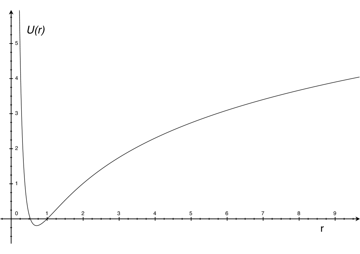
Figure 1. Potential $U$ in the case $a_{0}=1$ and $\lambda=-1$.

For every energy $E>U_{\rm min}$, the equation $U(r)=E$ has two distinct solutions. We infer (see e.g. [8]) that all the solutions to (3.2) are periodic, and the half-period is given by

$$\frac{T}{2}=\int_{r_{*}}^{r^{*}}\frac{dr}{\sqrt{E-U(r)}},$$

where $r_{*}<r^{*}$ are the two above mentionned solutions. Therefore, the amplitude of the corresponding (Gaussian) solution $u$ is time-periodic, and we naturally call such solutions breathers; see [41] for more details. Note however that only the amplitude is periodic, not the solution $u$ itself: in view of (3.1), $|b(t)|$ is periodic, but not $b(t)$, unless $|b_{0}|=1$ and $\operatorname{Im}A\equiv-0$.

As pointed out above, the relations $\beta_{0}=0$, $\alpha_{0}=-2\lambda$ imply $r\equiv 1$. This provides a stationary solution,

$$u(t,x)=\sqrt{e}\,e^{\lambda|x|^{2}}.$$

In view of the remarkable scaling property (1.6), and of the tensorization property discussed in the introduction, we infer the existence of infinitely many standing waves in ${\mathbb{R}}^{d}$ (we had assumed $d=1$ so far), parametrized by $\omega\in{\mathbb{R}}$ (related to $k\in{\mathbb{R}}$ in (1.6) through the relation $\omega=-\lambda\ln(k^{2})$),

$$u_{\omega}(t,x)=e^{i\omega t}e^{\frac{d}{2}-\frac{\omega}{2\lambda}}e^{\lambda|x|^{2}}.$$

These standing waves, discovered in [16] (see also [17]), are known as Gaussons. Given $\omega\in{\mathbb{R}}$ is arbitrary, for each prescribed mass $M$, there exists a (unique) Gausson whose mass is equal to $M$.

3.3. Dispersive case: $\lambda>0$

In this case, $r$ is strictly (but not uniformly) convex. We can prove the following: there exists $T\geqslant 0$ such that for $t\geqslant T$, $\ddot{r}>0$, and $r(t)\to\infty$ as $t\to\infty$. Therefore, the dynamics is expected to be well approximated by

$$\ddot{r}_{\rm eff}=\frac{2\lambda\alpha_{0}}{r_{\rm eff}}\quad(\alpha_{0}>0).$$

Multiply by $\dot{r}_{\rm eff}$ and integrate: since (at least) for $t\gg 1$, $\dot{r}_{\rm eff}>0$, we find

$$\dot{r}_{\rm eff}=\sqrt{C_{0}+4\lambda\alpha_{0}\ln r_{\rm eff}},$$

Separate variables:

$$\int^{r_{\rm eff}}\frac{dz}{\sqrt{C_{0}+4\lambda\alpha_{0}\ln z}}=t-T.$$

Set $y=\sqrt{C_{0}+4\lambda\alpha_{0}\ln z}$. The left hand side becomes

$$\frac{1}{2\lambda\alpha_{0}}\int^{Y}e^{(y^{2}-C_{0})/(4\lambda\alpha_{0})}dy.$$

The asymptotics of Dawson function (see e.g. [1]) yields, for any $x_{0}\in{\mathbb{R}}$,

$$\int_{x_{0}}^{x}e^{y^{2}}dy\mathop{\sim}\limits_{x\rightarrow\infty}\frac{1}{2x}e^{x^{2}}\Longrightarrow\frac{r_{\rm eff}}{\sqrt{C_{0}+4\lambda\alpha_{0}\ln r_{\rm eff}}}\mathop{\sim}\limits_{t\rightarrow\infty}t.$$

Since $r_{\rm eff}\to\infty$, $\displaystyle\frac{r_{\rm eff}}{\sqrt{4\lambda\alpha_{0}\ln r_{\rm eff}}}\mathop{\sim}\limits_{t\rightarrow\infty}t,$ hence

$$r_{\rm eff}(t)\mathop{\sim}\limits_{t\rightarrow\infty}2t\sqrt{\lambda\alpha_{0}\ln t}.$$

We note that $C_{0}$ has disappeared, at leading order. Thus, all the Gaussian solutions have the same asymptotic profile, with a nonstandard dispersion (enhanced compared to the standard one, by a logarithmic factor). Up to scaling the solution and changing initial data, we can simply consider $\displaystyle\ddot{\tau}=\frac{2\lambda}{\tau}$, with $\tau(0)=1$ and $\dot{\tau}(0)=0$. This yields a uniform dispersion in the case of Gaussian data. We will see that this dispersion is actually completely general, in the case $\lambda>0$.

4. Solitons

In this section, we always assume $\lambda<0$. The formal discussion presented in Section 1.3 suggests that when $\lambda<0$, dispersion is impossible. This has been proven rigorously by variational arguments by Thierry Cazenave:

Lemma 4.1 ([32]).

Let $\lambda<0$ and $k<\infty$ such that

$$L_{k}:=\{u\in W,\ \|u\|_{L^{2}({\mathbb{R}}^{d})}=1,\ E(u)\leqslant k\}\not=\emptyset\,.$$

Then $\displaystyle\inf_{{u\in L_{k}}\atop{1\leqslant p\leqslant\infty}}\|u\|_{L^{p}({\mathbb{R}}^{d})}>0.$

In view of the conservation of the mass and the energy, this implies that no solution is dispersive in the case $\lambda<0$ (otherwise an $L^{p}$-norm would go to zero for some $p>2$).

4.1. Gaussons

As we have seen above, we have explicit standing waves, called Gaussons, given by the formula

$$u_{\omega}(t,x)=e^{i\omega t}e^{\frac{d}{2}-\frac{\omega}{2\lambda}}e^{\lambda|x|^{2}}.$$

Due to the Galilean invariance (1.2), such solutions are not asymptotically stable: multiplying $u_{\omega}(0,x)$ by $e^{i{\mathbf{v}}\cdot x}$, for some small ${\mathbf{v}}$, is a small perturbation in $H^{1}$, but the drift in space, given by ${\mathbf{v}}t$, shows that the corresponding solution does not remain close to $u_{\omega}$ for all time. Even in the radial case (where Galilean invariance is absent), it is necessary to take phase shifts into account, as noticed in [32] by an explicit example on Gaussian data, which is related to (1.6): for $|\omega-\omega^{\prime}|\ll 1$, $u_{\omega}(0,\cdot)$ and $u_{\omega^{\prime}}(0,\cdot)$ are initial data which are close to each other in $H^{1}({\mathbb{R}}^{d})$, but of course the corresponding solutions $u_{\omega}$ and $u_{\omega^{\prime}}$ present a non-negligible phase shift e.g. for $(\omega-\omega^{\prime})t=\pi$. On the other hand, Gaussons are orbitally stable: this was proven in [32] for the radial case, and in [6] for the general case (the key variational step there is based on the logarithmic Sobolev inequality).

Theorem 4.2 ([32, 6]).

Let $\lambda<0$ and $\omega\in{\mathbb{R}}$. Set

$$\phi_{\omega}(x)=e^{\frac{d}{2}-\frac{\omega}{2\lambda}}e^{\lambda|x|^{2}}.$$

For any $\varepsilon>0$, there exists $\eta>0$ such that if $u_{0}\in W$ satisfies $\|u_{0}-\phi_{\omega}\|_{W}<\eta$, then the solution $u$ to (1.4) exists for all $t\in{\mathbb{R}}$, and

$$\sup_{t\in{\mathbb{R}}}\inf_{\theta\in{\mathbb{R}}}\inf_{y\in{\mathbb{R}}^{d}}\|u(t)-e^{i\theta}\phi_{\omega}(\cdot-y)\|_{W}<\varepsilon.$$

4.2. Superposition

Numerical experiments reported in [12] reveal dynamical properties which are fairly different from the phenomena observed in the case of a power-like nonlinearity, when solitons interact. In particular, two Gaussons centered far apart seem motionless over a long time of simulation. Each Gausson solves (1.4) exactly, but the equation being nonlinear, the sum of two Gaussons does not solve (1.4): there seems to be a rather strong superposition principle however. This was proven rigorously in [41], in a more general framework: starting from finitely many initial Gaussians (not necessarily Gaussons) with pairwise distances of order at least $1/\varepsilon$ (for $0<\varepsilon\ll 1$), the solution of (1.4) is well approximated by the sum of the corresponding solutions (computed in Section 3), over a time $o(\varepsilon^{-2})$. More precisely, the error is of order $e^{c_{0}t-c_{1}/\varepsilon^{2}}$ for some constants $c_{0},c_{1}>0$ expressed explicitly in [41].

At this stage, we emphasize an aspect which is crucial in the next section too: the logarithmic nonlinearity is not Lipschitz continuous at the origin, and in particular any linearization process becomes very delicate. To overcome this difficulty, the strategy employed in [41] consists in establishing fine properties of the logarithmic nonlinearity. Typically, the nonlinearity $F(z):=z\ln|z|^{2}$ satisfies, for $|z|,|z^{\prime}|\leqslant 1$, $z\not=0$,

(4.1) $$|F(z)-F(z^{\prime})|\leqslant|z-z^{\prime}|\left(6-\ln|z|^{2}\right).$$

The interest of this estimate lies in the fact that it is not symmetric in $(z,z^{\prime})$. This is crucial in order to estimate the source term in the equation solved by the difference between the exact solution and the sum of individual Gaussian solutions, which is of the form

$$u\ln|u|^{2}-\sum_{j=1}^{N}g_{j}\ln|g_{j}|^{2}.$$

4.3. Multigaussons

Again, we do not make complete statements here, and try to give a flavor of the corresponding result. Using the Galilean invariance, introduce, for some $k\geqslant 1$

$$G_{k}=\sum_{j=1}^{k}\Gamma_{j}(t,x),\quad\mathbb{B}_{k}=\sum_{j=1}^{k}B_{j}(t,x),$$

where the $\Gamma_{j}$’s are Gaussons associated with pairwise different velocities ${\mathbf{v}}_{j}$, and the $B_{j}$’s are (more general) breathers associated with pairwise different velocities ${\mathbf{v}}_{j}$. Unlike in [38], it is not assumed that the relative velocities ${\mathbf{v}}_{j}-{\mathbf{v}}_{k}$, $j\not=k$, are large. As evoked above, linearization is a delicate process here, and so, even though the following statement is reminiscent of [68] or [72] (for the modified KdV equation, an equation which is integrable), the approach must be adapted:

Theorem 4.3 ([43]).

Let $d\geqslant 1$ and $\lambda<0$.

• Multibreathers: there exists a unique solution $u\in C_{b}({\mathbb{R}};W)$ to (1.4), and $c,C>0$ such that

  $$\|u(t)-\mathbb{B}_{k}(t)\|_{L^{2}({\mathbb{R}}^{d})}\leqslant Ce^{-ct^{2}},\quad t\geqslant 0.$$

• Multigaussons: there exists a unique solution $u\in C_{b}({\mathbb{R}};\Sigma)$ to (1.4), $c,C>0$ such that

  $$\|u(t)-G_{k}(t)\|_{\Sigma}\leqslant Ce^{-ct^{2}},\quad t\geqslant 0.$$

We emphasize a few aspects, and refer to [43] for details:

• The construction is based on compactness techniques, as introduced in [68].

• The linearized operator around the Gausson seems to be nice, as it is a harmonic oscillator, whose eigenproperties are very well known. However, the logarithm is singular at zero, and so linearizing becomes a delicate matter. Like in the previous section, a clever use of (4.1) saves the day.

• The proof uses localized energy functionals involving a linearized functional, which is not the linearized energy.

5. Dispersive case

We now assume $\lambda>0$, and focus on the following result:

Theorem 5.1 ([31]).

Let $\lambda>0$. Introduce the solution $\tau\in C^{\infty}({\mathbb{R}})$ to

(5.1) $$\ddot{\tau}=\frac{2\lambda}{\tau}\,,\quad\tau(0)=1\,,\quad\dot{\tau}(0)=0\,.$$

Then, as $t\to\infty$, $\tau(t)\sim 2t\sqrt{\lambda\ln t}$ and $\dot{\tau}(t)\sim 2\sqrt{\lambda\ln t}$. For $u_{0}\in\Sigma\setminus\{0\}$, (1.4) has a unique solution $u\in L^{\infty}_{\rm loc}({\mathbb{R}};\Sigma))$. Introduce $\gamma(x):=e^{-|x|^{2}/2}$, and rescale the solution to $v=v(t,y)$ by setting

(5.2) $$u(t,x)=\frac{1}{\tau(t)^{d/2}}v\left(t,\frac{x}{\tau(t)}\right)\frac{\|u_{0}\|_{L^{2}({\mathbb{R}}^{d})}}{\|\gamma\|_{L^{2}({\mathbb{R}}^{d})}}\exp\Big{(}{i\frac{\dot{\tau}(t)}{\tau(t)}\frac{|x|^{2}}{2}}\Big{)}.$$

Then we have

(5.3) $$\sup_{t\geqslant 0}\left(\int_{{\mathbb{R}}^{d}}\left(1+|y|^{2}+\left|\ln|v(t,y)|^{2}\right|\right)|v(t,y)|^{2}dy+\frac{1}{\tau(t)^{2}}\|\nabla_{y}v(t)\|^{2}_{L^{2}}\right)<\infty,$$

(5.4) $$\int_{{\mathbb{R}}^{d}}\begin{pmatrix}1\\ y\\ |y|^{2}\end{pmatrix}|v(t,y)|^{2}dy\mathop{\longrightarrow}\limits_{t\rightarrow\infty}\int_{{\mathbb{R}}^{d}}\begin{pmatrix}1\\ y\\ |y|^{2}\end{pmatrix}\gamma^{2}(y)dy,$$

and

$$|v(t,\cdot)|^{2}\mathop{\rightharpoonup}\limits_{t\to\infty}\gamma^{2}\quad\text{weakly in }L^{1}({\mathbb{R}}^{d}).$$

The last bound in (5.3) shows that the phase introduced in (5.2) incorporates the main oscillations in the large time limit: since $\dot{\tau}(t)/\tau(t)\sim 1/t$ as $t\to\infty$, we recover the same oscillation (at leading order) as for the linear Schrödinger equation, see Section 1.1.2. On the other hand, the dispersive rate is different: the boundedness of the momentum of $v$ shows that $v$ is not dispersive, and the factor $t$ present in the expression of $A(t)$ in Section 1.1.2 has been replaced by $\tau(t)$. The dispersion of $u$ is thus enhanced by a logarithmic factor, compared to the standard dispersion. Finally, $|v(t,\cdot)|^{2}$ has a universal limit, which is reminiscent of the heat equation rather than of the Schrödinger equation.

As a consequence, the Sobolev norms of every nontrivial solutions are unbounded, providing a precise answer to a question asked in [18] regarding the growth of Sobolev norms for Hamiltonian nonlinear dispersive equations (see also e.g. [37, 44, 45, 50, 55, 73]):

Corollary 5.2.

Let $u_{0}\in\Sigma\setminus\{0\}$, and $0<s\leqslant 1$. As $t\to\infty$,

$$\left(\ln t\right)^{s/2}\lesssim\|u(t)\|_{\dot{H}^{s}({\mathbb{R}}^{d})}\lesssim\left(\ln t\right)^{s/2},$$

where $\dot{H}^{s}({\mathbb{R}}^{d})$ denotes the standard homogeneous Sobolev space.

Proof in the case $s=1$.

Differentiate (5.2) with respect to $x$:

$$\nabla u(t,x)=\frac{1}{\tau(t)^{d/2}}\nabla_{x}\left(v\left(t,\frac{x}{\tau(t)}\right)e^{i\frac{\dot{\tau}(t)}{\tau(t)}\frac{|x|^{2}}{2}}\right)$$

$$=\underbrace{\frac{1}{\tau(t)}\frac{1}{\tau(t)^{d/2}}\nabla_{y}v\left(t,\frac{x}{\tau(t)}\right)e^{i\frac{\dot{\tau}(t)}{\tau(t)}\frac{|x|^{2}}{2}}}_{\|\cdot\|_{L^{2}}=\frac{1}{\tau}\|\nabla v\|_{L^{2}}=\mathcal{O}(1).}+\underbrace{i\dot{\tau}\frac{1}{\tau(t)^{d/2}}\frac{x}{\tau}v\left(t,\frac{x}{\tau(t)}\right)e^{i\frac{\dot{\tau}(t)}{\tau(t)}\frac{|x|^{2}}{2}}}_{\|\cdot\|_{L^{2}}=\dot{\tau}\|yv\|_{L^{2}}\sim\dot{\tau}\|y\gamma\|_{L^{2}}\approx\sqrt{\ln t}},$$

where we have used (5.3) to control the first term, and (5.4) to show that the last factor is indeed of order $\dot{\tau}$. ∎

Remark 5.3.

For the case $0<s<1$, we refer to [31]. Essentially, the proof relies on [2, Lemma 5.1], which states the following (we simplify the original statement, which incorporates a semiclassical parameter): there exists a constant $K$ such that for all $s\in[0,1]$, all $u\in H^{1}({\mathbb{R}}^{d})$ and all $w\in W^{1,\infty}({\mathbb{R}}^{d})$,

$$\||w|^{s}u\|_{L^{2}}\leqslant\||D_{x}|^{s}u\|_{L^{2}}+\|(\nabla-iw)u\|_{L^{2}}^{s}\|u\|_{L^{2}}^{1-s}+K\left(1+\|\nabla w\|_{L^{\infty}}\right)\|u\|_{L^{2}}.$$

We then apply this inequality with $w$ the gradient of the quadratic oscillation in (5.3), $w(t,x)=\frac{\dot{\tau}(t)}{\tau(t)}x$.

Remark 5.4.

As pointed out by the editorial board, the function $\tau$, its asymptotic behavior, and the rescaling (5.2) were already present in [36], a reference we were not aware of.

Remark 5.5.

In the case of a defocusing power nonlinearity, (1.1) with $\lambda>0$, the conservation of the energy implies that the $H^{1}$-norm of $u$ is uniformly bounded in time, unlike in Corollary 5.2. Moreover, when ${\sigma}\geqslant 2/d$ is an integer, and $u\in{\mathcal{S}}({\mathbb{R}}^{d})$, all the Sobolev norms $\|u(t)\|_{H^{s}}$ are bounded. This result is natural, since in that case, $u$ is asymptotically linear and the linear flow $e^{i\frac{t}{2}\Delta}$ preserves the Sobolev norms $H^{s}$ (see e.g. [26]).

Remark 5.6.

These results remain valid when the logarithmic nonlinearity is perturbed by an energy-subcritical, defocusing powerlike nonlinearity,

$$i{\partial}_{t}u+\frac{1}{2}\Delta u=\lambda\ln\left(|u|^{2}\right)u+\mu|u|^{2{\sigma}}u,\quad u_{\mid t=0}=u_{0},$$

with $\mu>0$ and $0<{\sigma}<\frac{2}{(d-2)_{+}}$. Surprisingly enough, the logarithmic nonlinearity is thus the stronger in the above equation.

5.1. Elements of proof

5.1.1. A priori estimates

The key step is to change the unknown function in order to get coercivity. The change of unknown function is motivated by the explicit computations in the Gaussian case: at leading order, all the Gaussian solutions have the same dispersion, the same oscillations, and the same asymptotic profile. Theorem 5.1 states that these three properties are shared by all solutions.

Direct computations show that $v=v(t,y)$, given by (5.2), solves

$$i{\partial}_{t}v+\frac{1}{2\tau(t)^{2}}\Delta_{y}v=\lambda v\ln\left\lvert\frac{v}{\gamma}\right\rvert^{2}-\lambda dv\ln\tau+2\lambda v\ln\left(\frac{\|u_{0}\|_{L^{2}({\mathbb{R}}^{d})}}{\|\gamma\|_{L^{2}({\mathbb{R}}^{d})}}\right)\,,$$

where we recall that $\gamma(y)=e^{-|y|^{2}/2}$, and the initial datum for $v$ is

$$v_{\mid t=0}=v_{0}:=\frac{\|\gamma\|_{L^{2}({\mathbb{R}}^{d})}}{\|u_{0}\|_{L^{2}({\mathbb{R}}^{d})}}u_{0}.$$

Replacing $v$ with $ve^{-i\theta(t)}$ for

$$\theta(t)=\lambda d\int_{0}^{t}\ln\tau(s)ds-2\lambda t\ln(\|u_{0}\|_{L^{2}}/\|\gamma\|_{L^{2}}),$$

a change of unknown function which does not affect the conclusions of Theorem 5.1, we may assume that the last two terms are absent, and we focus our attention on

(5.5) $$i{\partial}_{t}v+\frac{1}{2\tau(t)^{2}}\Delta_{y}v=\lambda v\ln\left\lvert\frac{v}{\gamma}\right\rvert^{2},\quad v_{\mid t=0}=v_{0}\,.$$

The above equation is still Hamiltonian: introduce

$$\mathcal{E}(t):=\operatorname{Im}\int_{{\mathbb{R}}^{d}}\bar{v}(t,y){\partial}_{t}v(t,y)dy=\mathcal{E}_{\rm kin}(t)+\lambda\mathcal{E}_{\rm ent}(t)\,,$$

where

$$\mathcal{E}_{\rm kin}(t):=\frac{1}{2\tau(t)^{2}}\|\nabla_{y}v(t)\|_{L^{2}}^{2}$$

is the (modified) kinetic energy and

$$\mathcal{E}_{\rm ent}(t):=\int_{{\mathbb{R}}^{d}}|v(t,y)|^{2}\ln\left\lvert\frac{v(t,y)}{\gamma(y)}\right\rvert^{2}dy=\int_{{\mathbb{R}}^{d}}|v(t,y)|^{2}\ln\left\lvert{v(t,y)}\right\rvert^{2}dy+\int_{{\mathbb{R}}^{d}}|y|^{2}|v(t,y)|^{2}dy$$

is a relative entropy. Direct computations yield

(5.6) $$\dot{\mathcal{E}}=-2\frac{\dot{\tau}}{\tau}\mathcal{E}_{\rm kin}\,.$$

Remark 5.7.

The Csiszár-Kullback inequality reads (see e.g. [3, Th. 8.2.7]), for $f,g\geqslant 0$ with $\int f=\int g$,

$$\|f-g\|_{L^{1}({\mathbb{R}}^{d})}^{2}\leqslant 2\|f\|_{L^{1}({\mathbb{R}}^{d})}\int f(x)\ln\left(\frac{f(x)}{g(x)}\right)dx.$$

Since $|v|^{2}$ and $\gamma^{2}$ have the same $L^{1}$-norm, ${\mathcal{E}}_{\rm ent}\geqslant 0$: we will not actually use this piece of information, but this shows that if we could prove ${\mathcal{E}}_{\rm ent}(t)\to 0$ as $t\to\infty$ (which is established in the case of Gaussian initial data), then the weak convergence in the last point of Theorem 5.1 would become a strong convergence.

The following lemma resumes (5.3), and contains an extra integrability property:

Lemma 5.8.

Under the assumptions of Theorem 5.1,

$$\sup_{t\geqslant 0}\left(\int_{{\mathbb{R}}^{d}}\left(1+|y|^{2}+\left|\ln|v(t,y)|^{2}\right|\right)|v(t,y)|^{2}dy+\frac{1}{\tau(t)^{2}}\|\nabla_{y}v(t)\|^{2}_{L^{2}({\mathbb{R}}^{d})}\right)<\infty$$

and

(5.7) $$\int_{0}^{\infty}\frac{\dot{\tau}(t)}{\tau^{3}(t)}\|\nabla_{y}v(t)\|^{2}_{L^{2}({\mathbb{R}}^{d})}dt<\infty.$$

Proof.

Write the pseudo-energy $\mathcal{E}$ as $\mathcal{E}=\mathcal{E}_{+}+\mathcal{E}_{-}$, where $\mathcal{E}_{+}$ gathers the positive terms of $\mathcal{E}$,

$$\mathcal{E}_{+}(t)=\frac{1}{2\tau(t)^{2}}\|\nabla_{y}v(t)\|_{L^{2}}^{2}+\lambda\int_{|v|>1}|v|^{2}\ln|v|^{2}+\lambda\int_{{\mathbb{R}}^{d}}|y|^{2}|v|^{2},$$

and

$$\mathcal{E}_{-}(t)=\lambda\int_{|v|<1}|v|^{2}\ln|v|^{2}\leqslant 0.$$

Since $\mathcal{E}$ is nonincreasing,

$$\mathcal{E}_{+}(t)\leqslant\mathcal{E}(0)-\mathcal{E}_{-}(t)\leqslant\mathcal{E}(0)+C_{\varepsilon}\int_{|v|<1}|v|^{2-\varepsilon}\leqslant\mathcal{E}(0)+C_{\varepsilon}\int_{{\mathbb{R}}^{d}}|v|^{2-\varepsilon},$$

for any $0<\varepsilon<2$. Recalling (2.2) (with $\alpha=1$), and noting that $\|v(t)\|_{L^{2}}=\|v(0)\|_{L^{2}}(=\|\gamma\|_{L^{2}})$, we obtain a control of the form

$$\mathcal{E}_{+}(t)\leqslant\mathcal{E}(0)+C\mathcal{E}_{+}(t)^{d\epsilon/2},$$

hence $\mathcal{E}_{+}\in L^{\infty}({\mathbb{R}}_{+})$ by picking $\varepsilon>0$ sufficiently small. Then $\mathcal{E}_{-}\in L^{\infty}({\mathbb{R}}_{+})$, hence $\mathcal{E}\in L^{\infty}({\mathbb{R}}_{+})$, and (5.7) by just saying that $\dot{\mathcal{E}}$ is integrable. ∎

5.1.2. Center of mass

Adapting the computation of [39], introduce

$$I_{1}(t):=\operatorname{Im}\int_{{\mathbb{R}}^{d}}\overline{v}(t,y)\nabla_{y}v(t,y)dy\,,\quad I_{2}(t):=\int_{{\mathbb{R}}^{d}}y|v(t,y)|^{2}dy\,.$$

We compute:

$$\dot{I}_{1}=-2\lambda I_{2}\,,\qquad\dot{I}_{2}=\frac{1}{\tau(t)^{2}}I_{1}\,.$$

Set $\tilde{I}_{2}=\tau I_{2}$: $\ddot{\tilde{I}}_{2}=0$, hence

$$I_{2}(t)=\frac{1}{\tau(t)}\left(\dot{\tilde{I}}_{2}(0)t+\tilde{I}_{2}(0)\right)=\frac{1}{\tau(t)}\left(-I_{1}(0)t+I_{2}(0)\right)=\mathcal{O}\left(\frac{1}{\sqrt{\ln t}}\right)\,.$$

In particular, $\displaystyle\int_{{\mathbb{R}}^{d}}y|v(t,y)|^{2}dy\mathop{\longrightarrow}\limits_{t\rightarrow\infty}0=\int_{{\mathbb{R}}^{d}}y\gamma(y)^{2}dy.$ If $I_{1}(0)\not=0$, we also have

$$I_{1}(t)\mathop{\sim}\limits_{t\rightarrow\infty}c\frac{t}{\sqrt{\ln t}},$$

while if $I_{1}(0)=0\not=I_{2}(0)$,

$$I_{1}(t)\mathop{\sim}\limits_{t\rightarrow\infty}\tilde{c}\sqrt{\ln t}.$$

Remark 5.9.

In view of Cauchy-Schwarz inequality,

$$|I_{1}(t)|\leqslant\|v\|_{L^{2}}\|\nabla_{y}v\|_{L^{2}}=\|\gamma\|_{L^{2}}\|\nabla_{y}v\|_{L^{2}}.$$

So unless the initial data are centered in zero in phase space ($I_{1}(0)=I_{2}(0)=0$),

$$\|\nabla_{y}v(t)\|_{L^{2}}\mathop{\longrightarrow}\limits_{t\rightarrow\infty}\infty,$$

suggesting that $v$ is rapidly oscillatory: in general, (5.2) filters out the leading order oscillations only, in the limit $t\to\infty$. A careful examination of the computations in the Gaussian case leads to the same conclusion. This explains why, in Theorem 5.1, the main results concern the modulus of $v$, and no other quantity (that would involve the argument of $v$).

5.1.3. Second order momentum

Introduce $\displaystyle A=\operatorname{Im}\int v\,y\cdot\nabla_{y}\bar{v}.$ The estimate (5.3) and Cauchy-Schwarz inequality yield: $|A|\leqslant\|yv\|_{L^{2}}\|\nabla v\|_{L^{2}}\lesssim\tau(t)$.

Use the conservation of the energy of $u$, and rewrite the energy in terms of $v$, via (5.2):

$$\frac{d}{dt}\Bigg{(} \underbrace{E_{\rm kin}}_{=\mathcal{O}(1)}+\frac{(\dot{\tau})^{2}}{2}\int|y|^{2}|v|^{2}-\underbrace{\frac{\dot{\tau}}{\tau}A}_{=\mathcal{O}(\dot{\tau})}+\underbrace{\lambda\int|v|^{2}\ln|v|^{2}}_{=\mathcal{O}(1)}-\lambda d\ln\tau\int|v|^{2}$$

$$+\underbrace{2\lambda\|\gamma\|_{L^{2}}^{2}\ln\left(\frac{\|u_{0}\|_{L^{2}}}{\|\gamma\|_{L^{2}}}\right)}_{=\mathcal{O}(1)}\Bigg{)}=0,$$

where we have used (5.3) for the a priori estimates. We infer

$$\frac{(\dot{\tau})^{2}}{2}\int|y|^{2}|v|^{2}-\lambda d\ln\tau\int|v|^{2}=\mathcal{O}(\dot{\tau}).$$

But multiplying (5.1) by $\dot{\tau}$ and integrating, we find $(\dot{\tau})^{2}=4\lambda\ln\tau$, and $\|v\|_{L^{2}}^{2}=\|\gamma\|_{L^{2}}^{2}=\frac{2}{d}\|y\gamma\|_{L^{2}}^{2}$, so we conclude

$$\|yv(t)\|_{L^{2}}^{2}-\|y\gamma\|_{L^{2}}^{2}=\mathcal{O}\left(\frac{1}{\sqrt{\ln t}}\right).$$

5.1.4. Universal profile

The proof of the weak convergence of $|v(t,\cdot)|^{2}$ to $\gamma^{2}$ relies on a hydrodynamical formulation of (5.5), based on the Madelung transform, which relates (nonlinear) Schrödinger equations to some equations from compressible fluid mechanics (see for instance the survey [30]). Formally, this amounts to a polar factorization of $v$,

$$v=\sqrt{\rho}e^{i\phi}.$$

The fluid velocity is then given by $\nabla\phi$. However, such a decomposition is obviously delicate when $v$ (or, equivalently, $\rho$) becomes zero. The rigorous approach consists in introducing

$$\rho=|v|^{2},\quad J=\operatorname{Im}\bar{v}\nabla v.$$

From a fluid mechanical perspective, we consider the momentum $J$ instead of the velocity: this is standard in compressible fluid mechanics. Plugging this decomposition into (5.5) and separating real and imaginary parts, we find:

$$\left\{\begin{aligned} &{\partial}_{t}\rho+\frac{1}{\tau^{2}}\nabla\cdot J=0,\\ &{\partial}_{t}J+\lambda\nabla\rho+2\lambda y\rho=\frac{1}{4\tau^{2}}\Delta\nabla\rho-\frac{1}{\tau^{2}}\nabla\cdot\operatorname{Re}\left(\nabla v\otimes\nabla\bar{v}\right).\end{aligned}\right.$$

To guess the result, consider the baby model:

$$\left\{\begin{aligned} &{\partial}_{t}\rho+\frac{1}{\tau^{2}}\nabla\cdot J=0,\\ &{\partial}_{t}J+\lambda\nabla\rho+2\lambda y\rho=0.\end{aligned}\right.$$

We can write an equation involving $\rho$ only, by just writing ${\partial}_{t}\nabla\cdot J=\nabla\cdot{\partial}_{t}J$:

$${\partial}_{t}\left(\tau^{2}{\partial}_{t}\rho\right)=\lambda\nabla\cdot\left(\nabla+2y\right)\rho=:\lambda L\rho,$$

where $L$ is the Fokker-Planck operator associated to the harmonic potential. Note that $\tau^{2}\ll(\dot{\tau}\tau)^{2}$: define $s$ such that $\displaystyle\frac{\dot{\tau}\tau}{\lambda}{\partial}_{t}={\partial}_{s}\,,$ that is

$$s=\int\frac{\lambda}{\dot{\tau}\tau}=\int\frac{\ddot{\tau}}{2\dot{\tau}}=\frac{1}{2}\ln\dot{\tau}(t)\,.$$

Notice that

$$s\sim\frac{1}{4}\ln\ln t\,,\quad t\to\infty\,.$$

Then again discarding formally lower order terms we find

$${\partial}_{s}\rho=L\rho.$$

Remark 5.10.

Recall that $\rho(t,y)=|v(t,y)|^{2}$: the previous computations have shown

$$\int_{{\mathbb{R}}^{d}}\begin{pmatrix}1\\ y\\ |y|^{2}\end{pmatrix}\rho(t,y)dy=\int_{{\mathbb{R}}^{d}}\begin{pmatrix}1\\ y\\ |y|^{2}\end{pmatrix}\gamma^{2}(y)dy+\mathcal{O}\left(\frac{1}{\sqrt{\ln t}}\right).$$

We have just derived formally:

$${\partial}_{s}\rho=L\rho,\quad L=\nabla\cdot\left(\nabla+2y\right).$$

For such Fokker–Planck equation, convergence to equilibrium is known thanks to (5.3) ([7]),

$$\|\rho(s)-\gamma^{2}\|_{L^{1}}\lesssim e^{-Cs}\|\rho_{0}-\gamma^{2}\|_{L^{1}}.$$

The constant $C$ stems from a spectral gap, which is, in the present case of a Fokker-Planck operator associated to the harmonic potential, $C=2$. Both aspects coincide, since

$$s\sim\frac{1}{4}\ln\ln t\,,\quad t\to\infty,\quad\text{hence}\quad e^{-2s}\sim\frac{1}{\sqrt{\ln t}}.$$

This is a hint that the new time variable $s$ is well adapted. Back to the complete hydrodynamical system, introduce the time variable $s$, $\tilde{\rho}(s,y):=\rho(t,y)$:

$${\partial}_{s}\tilde{\rho}-\frac{2\lambda}{(\dot{\tau})^{2}}{\partial}_{s}\tilde{\rho}+\frac{\lambda}{(\dot{\tau})^{2}}{\partial}_{s}^{2}\tilde{\rho}=L\tilde{\rho}-\frac{1}{4\lambda\tau^{2}}\Delta^{2}\tilde{\rho}-\frac{1}{\tau^{2}}\nabla\cdot\nabla\cdot\operatorname{Re}\left(\nabla v\otimes\nabla\bar{v}\right).$$

For $s\in[-1,2]$ and an arbitrary sequence $s_{n}\to\infty$, set $\tilde{\rho}_{n}(s,y)=\tilde{\rho}(s+s_{n},y).$ By De la Vallée-Poussin and Dunford–Pettis theorems, we have some weak compactness in $L^{1}$, hence, up to a subsequence,

$$\tilde{\rho}_{n}\rightharpoonup\tilde{\rho}_{\infty}\text{ in }L^{p}_{s}(-1,2;L^{1}_{y}),\quad\forall p\in[1,\infty).$$

Passing to the limit in the equation for $\tilde{\rho}$ (see [31] for details),

$${\partial}_{s}\tilde{\rho}_{\infty}=L\tilde{\rho}_{\infty}\text{ in }\mathcal{D}^{\prime}\left((-1,2)\times{\mathbb{R}}^{d}\right).$$

Since $J=\operatorname{Im}\bar{v}\nabla_{y}v$, (5.7) yields

$$\frac{\dot{\tau}}{\tau}\tilde{J}\in L^{2}_{s}L^{1}_{y},\quad\text{hence }\frac{\dot{\tau}}{\tau}\nabla\cdot\tilde{J}_{n}\mathop{\longrightarrow}\limits_{n\rightarrow\infty}0\quad\text{in }L^{2}(-1,2;W^{-1,1}).$$

Therefore, ${\partial}_{s}\tilde{\rho}_{\infty}=0$.

On the other hand, as evoked above, it is known from [7] that any solution to

$${\partial}_{s}\tilde{\rho}_{\infty}=L\tilde{\rho}_{\infty}$$

satisfying the a priori estimates of Lemma 5.8 converges for large time

$$\lim_{s\to\infty}\|\tilde{\rho}_{\infty}(s)-\gamma^{2}\|_{L^{1}({\mathbb{R}}^{d})}=0.$$

Since we have seen that ${\partial}_{s}\tilde{\rho}_{\infty}=0$, we infer $\tilde{\rho}_{\infty}=\gamma^{2}$. Thus, the limit is unique, and no extraction is needed:

$$\tilde{\rho}(s)\mathop{\rightharpoonup}\limits_{s\to\infty}\gamma^{2}\quad\text{weakly in }L^{1}({\mathbb{R}}^{d}).$$

Remark 5.11.

Some information is lost when approximating the original hydrodynamical system by a Fokker-Planck equation: this is the reason why only a weak convergence is obtained. This should not be too surprising, as the Fokker-Planck equation is parabolic, while we started from a Hamiltonian equation. On the other hand, in [42], by changing the strategy of proof, the convergence is improved: Denoting by $W_{1}$ the Wasserstein distance, there exists $C$ such that

$$W_{1}\left(\frac{|v(t)|^{2}}{\pi^{d/2}},\frac{\gamma^{2}}{\pi^{d/2}}\right)\leqslant\frac{C}{\sqrt{\ln t}},\quad t\geqslant e.$$

We recall that for $\nu_{1}$ and $\nu_{2}$ probability measures, the Wasserstein distance is defined by

$$W_{p}(\nu_{1},\nu_{2})=\inf\left\{\left(\int_{{\mathbb{R}}^{d}\times{\mathbb{R}}^{d}}|x-y|^{p}d\mu(x,y)\right)^{1/p};\quad(\pi_{j})_{\sharp}\mu=\nu_{j}\right\},$$

where $\mu$ varies among all probability measures on ${\mathbb{R}}^{d}\times{\mathbb{R}}^{d}$, and $\pi_{j}:{\mathbb{R}}^{d}\times{\mathbb{R}}^{d}\to{\mathbb{R}}^{d}$ denotes the canonical projection onto the $j$-th factor. See e.g. [78]. In the case $p=1$, the Wasserstein distance, corresponding to the Kantorovich-Rubinstein metric, is also characterized by

$$W_{1}(\nu_{1},\nu_{2})=\sup\left\{\int_{{\mathbb{R}}^{d}}\Phi d(\mu_{1}-\mu_{2}),\ \Phi\in C({\mathbb{R}}^{d};{\mathbb{R}}),\ \operatorname{Lip}(\Phi)\leqslant 1\right\},$$

and it is this point of view which is adopted in [42]. The question of the strong convergence, in L¹, of $|v|^{2}$ toward $\gamma^{2}$ remains open for non-Gaussian initial data.

6. From NLS to compressible fluids

We have seen that the end of the proof of Theorem 5.1 relies on a hydrodynamical point of view. This suggests that we might consider models from fluid mechanics from the very start (instead of (1.4)), and see how what has been understood on the Schrödinger side can be exported to the fluid mechanical side. Essentially, Theorem 5.1 has an exact counterpart in fluid mechanics, up to two important remarks:

• The direct analogue of (1.4) in fluid mechanics is the Korteweg equation (via Madelung transform): we may have or not have the capillary term (Korteweg or Euler), and we may add a quantum Navier-Stokes term.

• The existence theory is much easier in the Schrödinger case, (1.4), than for fluids.

Consider the solution $u$ to (1.1), and resume the Madelung transform, now directly for $u$:

$$\rho=|u|^{2},\quad j=\operatorname{Im}\bar{u}\nabla u.$$

The unknown $(\rho,j)$ solves the Korteweg system:

$$\left\{\begin{aligned} &{\partial}_{t}\rho+\nabla\cdot j=0,\\ &{\partial}_{t}j+\nabla\left(\frac{j\otimes j}{\rho}\right)+\nabla\left(\rho^{\gamma}\right)=\frac{1}{2}\rho\nabla\left(\frac{\Delta\sqrt{\rho}}{\sqrt{\rho}}\right),\end{aligned}\right.$$

provided that we require

$$\lambda=\frac{\gamma}{\gamma-1},\quad{\sigma}=\frac{\gamma-1}{2}.$$

The capillarity term (right-hand side of the second equation), involving the term $\frac{1}{2}\left(\frac{\Delta\sqrt{\rho}}{\sqrt{\rho}}\right)$, also known as quantum pressure or Bohm potential in quantum mechanics, can be written in several fashions, e.g.:

$$\rho\nabla\left(\frac{\Delta\sqrt{\rho}}{\sqrt{\rho}}\right) =\frac{1}{2}\nabla\cdot\left(\rho\nabla^{2}\ln\rho\right)=\nabla\cdot\left(\sqrt{\rho}\nabla^{2}\sqrt{\rho}-\nabla\sqrt{\rho}\otimes\nabla\sqrt{\rho}\right)$$

$$=\frac{1}{2}\nabla\Delta\rho-2\nabla\cdot\left(\nabla\sqrt{\rho}\otimes\nabla\sqrt{\rho}\right).$$

See for instance [4, 30]. Either of these formulas may be used, typically when constructing solutions to the Korteweg equation, according to the level of regularity considered, and the presence or absence of vacuum.

When $\gamma>1$, the pressure law $P(\rho)=\rho^{\gamma}$ corresponds to polytropic fluids, while for $\gamma=1$, the fluid is isothermal. We note that to get a correspondence with fluid mechanics, the nonlinearity in Schrödinger equations comes with some coupling constant $\lambda>0$ (defocusing case).

7. The limit $\gamma\to 1$

From the above identification between ${\sigma}$ and $\gamma$, passing to the limit $\gamma\to 1$ is clear, at least formally, in the equations from fluid mechanics. On the other hand, it is not obvious to determine the “natural” limit for Equation (1.1) when ${\sigma}\to 0$. Madelung transform, as we have seen before, suggests that the “good” limit is

$$|u|^{2{\sigma}}u\to\ln(|u|)u\quad\text{as}\quad{\sigma}\to 0.$$

We mention [79], where it is shown that the ground state of

$$-\frac{1}{2}\Delta\phi+\omega\phi=|\phi|^{2{\sigma}}\phi$$

converges, as ${\sigma}\to 0$, to the ground state of

$$-\frac{1}{2}\Delta\phi+\omega\phi=\phi\ln|\phi|,$$

that is, the Gausson (up to invariants). This case, corresponding to the assumption $\lambda<0$, gives more credit to the above discussion.

Apart from this very specific case, it is difficult to give a rigorous meaning to the limit $\gamma\to 1$, or even construct solutions the case $\gamma=1$. In the case of (1.1), we have seen that the (nonlinear) potential energy is

$$\frac{\lambda}{{\sigma}+1}\int_{{\mathbb{R}}^{d}}|u(t,x)|^{2{\sigma}+2}dx,$$

and becomes, in the case of (1.4),

$$\lambda\int_{{\mathbb{R}}^{d}}|u(t,x)|^{2}\left(\ln|u(t,x)|^{2}-1\right)dx.$$

It has no longer a definite sign. In the fluid case, using the conservation of mass, the standard entropy in the isothermal case reads

$$\int_{{\mathbb{R}}^{d}}\rho(t,x)\ln\rho(t,x)dx,$$

and we naturally face the same issue. There is however a major difference regarding the Cauchy problem: (1.1) is semilinear (for ${\sigma}<\frac{2}{(d-2)_{+}}$, it is solved in $H^{1}({\mathbb{R}}^{d})$ by using a fixed point argument, and the nonlinearity is viewed as a perturbation, see e.g. [33]), while the above Korteweg equation is quasilinear (nonlinear terms cannot be viewed as perturbations, unless one works with analytic regularity). The Cauchy problem is in general still a major issue for the equations of compressible fluid mechanics which we now discuss, in the sense that the optimal assumptions to construct weak solutions are not always known; see e.g. [71] and references therein. For this reason, we distinguish rigidity results (“if theorem”) and the construction of weak solutions.

On the other hand, the presence of a pressure term of isothermal form in the large time limit can be guessed as follows. Consider more generally a barotropic (convex) pressure law $P(\rho)$, not necessarily equal to $\rho^{\gamma}$. Since the gradient of the pressure is involved, the value of $P(0)$ is irrelevant from a mathematical point of view, and we assume $P(0)=0$. If the density $\rho$ is dispersive in the large time limit, then the Taylor expansion of $P$ at zero determines the large time behavior:

$$P(\rho)\mathop{\sim}\limits_{\rho\rightarrow 0}P^{\prime}(0)\rho+\frac{1}{2}P^{\prime\prime}(0)\rho^{2}+\dots$$

If $P^{\prime}(0)>0$, then isothermal effects are present at leading order, while if $P^{\prime}(0)=0$, the dynamics corresponds to polytropic fluids. This is another way, probably more natural, to interpret Remark 5.6; see Remark 9.2.

8. Isothermal fluids: setting

From now on, we no longer write any Schrödinger equation, and $u$ denotes the fluid velocity, whose rigorous definition requires some care (as we have slightly evoked before), and which corresponds to the momentum divided by the density,

$$u=\frac{j}{\rho},$$

outside of vacuum, that is for $\rho>0$ ($\rho\geqslant 0$ in general). We consider

(8.1) $$\left\{\begin{aligned} &{\partial}_{t}\rho+\nabla\cdot(\rho u)=0,\\ &{\partial}_{t}(\rho u)+\nabla\cdot(\rho u\otimes u)+\nabla\rho=\frac{\varepsilon^{2}}{2}\rho\nabla\left(\frac{\Delta\sqrt{\rho}}{\sqrt{\rho}}\right)+\nu\nabla\cdot(\rho{\mathbb{D}}u),\end{aligned}\right.$$

with a capillarity $\varepsilon\geqslant 0$, a viscosity $\nu\geqslant 0$, and where ${\mathbb{D}}u=\frac{1}{2}(\nabla u+\nabla u^{\top})$ denotes the symmetric part of $\nabla u$. The first term of the right-hand side corresponds to capillarity (Korteweg term), and the second is a quantum Navier-Stokes correction, see [24]: contrary to the Newtonian case involving $\nu\Delta u$ (see e.g. [40, 66]), the viscosity can be thought of as linear in $\rho$; see [22, 23] for more general models and their analysis.

We shall not detail here the notion of solution adopted in [28, 27], and present the main results or ideas in a rather superficial way.

Formally, the mass is conserved in (8.1),

$$\frac{d}{dt}\int_{{\mathbb{R}}^{d}}\rho(t,x)dx=0,$$

and the energy

(8.2) $$E(t)=\frac{1}{2}\int_{{\mathbb{R}}^{d}}\rho|u|^{2}dx+\frac{\varepsilon^{2}}{2}\int|\nabla\sqrt{\rho}|^{2}dx+\int_{{\mathbb{R}}^{d}}\rho\ln\rho\,dx,$$

satisfies

(8.3) $$\dot{E}(t)=-\nu\int_{{\mathbb{R}}^{d}}\rho|\mathbb{D}u|^{2}dx.$$

We do not write the dependence of the integrated functions upon $(t,x)$ to shorten notations.

Remark 8.1 (Explicit solutions).

If $\rho_{0}$, the initial datum for $\rho$, is Gaussian, and if $u_{0}$ (initial velocity) is affine (think of $u_{0}$ as the gradient of the argument of a complex Gaussian), then we have explicit solutions: $\rho(t,\cdot)$ is Gaussian for all $t\geqslant 0$, $u(t,\cdot)$ is affine, and their time-dependent coefficients are given by explicit ordinary differential equations. Surprisingly enough, at leading order, the large time behavior of the solutions to these ordinary differential equations is independent of $\varepsilon,\nu\geqslant 0$, and the analysis presented in Section 3 is generalized in [28].

9. Rigidity in isothermal fluids

The end of the proof of Theorem 5.1 relies on a hydrodynamical approach, suggesting that some results remain valid if we start from the isothermal Korteweg equation. The argument presented in Section 5.1.4 suggests that the capillary term has no influence in the large time behavior at leading order: assuming $\varepsilon>0$ or $\varepsilon=0$ in (8.1) is not expected to change the large time description. More surprisingly, the presence of the quantum Navier-Stokes correction has no influence either: we may suppose $\nu=0$ or $\nu>0$.

In view of (5.2) and Madelung transform, we change the unknown functions $(\rho,u)$ to $(R,U)$ through the relations

(9.1) $$\rho(t,x)=\frac{1}{\tau(t)^{d}}R\left(t,\frac{x}{\tau(t)}\right)\frac{\|\rho_{0}\|_{L^{1}}}{\|\Gamma\|_{L^{1}}},\quad u(t,x)=\frac{1}{\tau(t)}U\left(t,\frac{x}{\tau(t)}\right)+\frac{\dot{\tau}(t)}{\tau(t)}x,$$

where we denote by $y$ the spatial variable for $R$ and $U$. The function $\tau$ is the same as in Theorem 5.1, given by (5.1). The function $\Gamma$ is defined by $\Gamma(y)=e^{-|y|^{2}}$; in other words, $\Gamma=\gamma^{2}$ as defined in Theorem 5.1. The system (8.1) becomes, in terms of these new unknowns,

(9.2) $$\left\{\begin{aligned} &{\partial}_{t}R+\frac{1}{\tau^{2}}\nabla\cdot\left(RU\right)=0,\\ &{\partial}_{t}(RU)+\frac{1}{\tau^{2}}\nabla\cdot(RU\otimes U)+2\kappa yR+\nabla R\\ &\phantom{{\partial}_{t}(Rw)+\frac{1}{\tau^{2}}\nabla}=\frac{\varepsilon^{2}}{2\tau^{2}}R\nabla\left(\frac{\Delta\sqrt{R}}{\sqrt{R}}\right)+\frac{\nu}{\tau^{2}}\nabla\cdot(R\mathbb{D}U)+\nu\frac{\dot{\tau}}{\tau}\nabla R.\end{aligned}\right.$$

We define the pseudo-energy $\mathcal{E}$ of the system (9.2) by

(9.3) $$\mathcal{E}(t):=\frac{1}{2\tau^{2}}\int R|U|^{2}+\frac{\varepsilon^{2}}{2\tau^{2}}\int|\nabla\sqrt{R}|^{2}+\int(R|y|^{2}+R\ln R),$$

which formally satisfies

(9.4) $$\dot{\mathcal{E}}(t)=-\mathcal{D}(t)-\nu\frac{\dot{\tau}(t)}{\tau(t)^{3}}\int R(t,y)\nabla\cdot U(t,y)dy,$$

where the dissipation $\mathcal{D}(t)$ is defined by

(9.5) $$\mathcal{D}(t):=\frac{\dot{\tau}}{\tau^{3}}\int R|U|^{2}+\varepsilon^{2}\frac{\dot{\tau}}{\tau^{3}}\int|\nabla\sqrt{R}|^{2}+\frac{\nu}{\tau^{4}}\int R|\mathbb{D}U|^{2}.$$

Mimicking the proof of Lemma 5.8, it is natural to expect that each term in $\mathcal{E}$ is bounded (recall that $\mathcal{E}$ is not signed, because of the logarithm), and that $\dot{\mathcal{E}}$ is integrable. This is formally a natural assumption, but as the Cauchy problem is a delicate issue, the following result remains an “if theorem” in most cases.

Theorem 9.1 ([28]).

Let $\varepsilon,\nu\geqslant 0$, and let $(R,U)$ be a global weak solution of (9.2).

1. If $\int_{0}^{\infty}\mathcal{D}(t)\,dt<\infty,$ then

   $$\int_{{\mathbb{R}}^{d}}yR(t,y)dy\mathop{\longrightarrow}\limits_{t\rightarrow\infty}0\quad\text{and}\quad\left|\int_{{\mathbb{R}}^{d}}(RU)(t,y)dy\right|\mathop{\longrightarrow}\limits_{t\rightarrow\infty}\infty,$$

   unless $\int yR(0,y)dy=\int(RU)(0,y)dy=0$, a case where

   $$\int_{{\mathbb{R}}^{d}}yR(t,y)dy=\int_{{\mathbb{R}}^{d}}(RU)(t,y)dy\equiv 0.$$

2. If $\displaystyle\sup_{t\geqslant 0}\mathcal{E}(t)+\int_{0}^{\infty}\mathcal{D}(t)dt<\infty,$ then $R(t,\cdot)\rightharpoonup\Gamma$ weakly in $L^{1}({\mathbb{R}}^{d})$ as $t\to\infty$.

3. If $\displaystyle\sup_{t\geqslant 0}\mathcal{E}(t)<\infty$ and the energy $E$ defined by (8.2) satisfies $E(t)=o\left(\ln t\right)$ as $t\to\infty$, then

   $$\int_{{\mathbb{R}}^{d}}|y|^{2}R(t,y)dy\mathop{\longrightarrow}\limits_{t\rightarrow\infty}\int_{{\mathbb{R}}^{d}}|y|^{2}\Gamma(y)dy.$$

Essentially, the proof is based on arguments similar to those sketched in Section 5.1. As evoked above, it is a bit of a surprise that the Navier-Stokes term goes through the arguments, and we refer to [28] for details.

Remark 9.2.

In the same spirit as the discussion at the end of Section 7, the pressure law considered in [28] is more general than exactly isothermal: we assume that $P\in C^{1}([0,\infty[;{\mathbb{R}}_{+})\cap C^{2}(]0,\infty[;{\mathbb{R}}_{+})$, and $P$ is convex, with $P^{\prime}(0)>0$.

10. On the existence of weak solutions

As already evoked, constructing solutions in compressible fluid mechanics is a difficult question. In the polytropic Euler equation ($\gamma>1$), a suitable change of unknown function (consider $\rho^{\frac{\gamma-1}{2}}$ instead of $\rho$) makes the system hyperbolic symmetric, so the Cauchy problem can be solved in Sobolev spaces with sufficiently high regularity, but finite time blow-up occurs, typically when starting from smooth, compactly supported data, [67, 35]. Global, smooth solutions are constructed for suitable affine velocities: [74, 49]. In the case of Korteweg equation, the link with nonlinear Schrödinger equations has been exploited in [14], leading to further developments, e.g. [4, 5, 9, 10]. In the presence of the quantum Navier-Stokes correction, many results are available, regarding the existence of weak solutions, still for $\gamma>1$; see e.g. [20, 46, 47, 62, 64, 76], and [71] for a survey. However, in the isothermal case $\gamma=1$, far less is known: we refer to [65] for the one-dimensional Euler equation, [62] for the quantum Navier-Stokes on ${\mathbb{T}}^{d}$ for $d\leqslant 2$.

In [27], we construct weak solutions to (8.1) in the presence of viscosity, $\nu>0$. We emphasize two aspects in this construction, which seem to be the most important contributions of this work:

• We consider solutions on the whole space ${\mathbb{R}}^{d}$, while most of the previous references assume a periodic setting, $x\in{\mathbb{T}}^{d}$ ($x\in{\mathbb{R}}$ in [65]).

• We gain positivity properties by working on the intermediary system (9.2).

Both points are intimately connected, as the change of unknown functions (9.1) involves a time-dependent rescaling. The reasons why most of the references consider the periodic setting $x\in{\mathbb{T}}^{d}$ seem to be mostly that compactness in space then comes from free, and integrations by parts can be performed freely. The periodic case is also rather convenient for approximating, among others in Lebesgue spaces, the initial density by a density bounded away from zero, a step which would require some modification on ${\mathbb{R}}^{d}$. Note also that this property is classically propagated by the flow in a suitable regularized continuity equation (see e.g. [40, 62]), and such a property is needed in the presence of cold pressure and regularizing terms (see e.g. [47, 77]).

For these reasons, to construct a solution $(R,U)$ to (9.2) on ${\mathbb{R}}^{d}$, we first replace ${\mathbb{R}}^{d}$ with a periodic box ${\mathbb{T}}^{d}_{\ell}$ of size $\ell>0$, where $\ell$ is aimed at going to infinity at the last step of the proof.

We refer to [27] for the details, and conclude this section by pointing out another important tool, which has proven very useful in the context of compressible Navier-Stokes equations with a density-dependent velocity, known as BD-entropy, after [19, 21]. It involves an effective velocity, which reads $U+\nu\nabla\ln R$ in the case of (9.2):

$${\mathcal{E}}_{\rm BD}(R,U)=\frac{1}{2\tau^{2}}\int_{{\mathbb{R}}^{d}}\left(R|U+\nu\nabla\log R|^{2}+\varepsilon^{2}|\nabla\sqrt{R}|^{2}\right)+\int_{{\mathbb{R}}^{d}}\left(R|y|^{2}+R\log R\right).$$

The evolution of this BD-entropy is given formally, for $t\geqslant 0$, by

(10.1) $${\mathcal{E}}_{\rm BD}(R,U)(t) +\int_{0}^{t}{\mathcal{D}}_{\rm BD}(R,U)(s)ds$$

$$={\mathcal{E}}_{\rm BD}(R_{0},U_{0})+\nu\int_{0}^{t}\frac{2d}{\tau^{2}}\int_{{\mathbb{R}}^{d}}R+\nu\int_{0}^{t}\frac{\dot{\tau}}{\tau^{3}}\int_{{\mathbb{R}}^{d}}R\nabla\cdot U,$$

where the above dissipation is defined by

(10.2) $${\mathcal{D}}_{\rm BD}(R,U) =\frac{\dot{\tau}}{\tau^{3}}\int\left(R|U|^{2}+\varepsilon^{2}|\nabla\sqrt{R}|^{2}\right)+\frac{\nu}{\tau^{4}}\int_{{\mathbb{R}}^{d}}R|\mathbb{A}U|^{2}$$

$$\quad+\frac{\nu\varepsilon^{2}}{\tau^{4}}\int R|\nabla^{2}\log R|^{2}+\frac{4\nu}{\tau^{2}}\int|\nabla\sqrt{R}|^{2},$$

with $\mathbb{A}U:=\frac{1}{2}(\nabla U-\nabla U^{\top})$ the skew-symmetric part of $\nabla U.$ Hence putting together the energy and the BD-entropy equalities, it holds

$$\mathcal{E}(t)+{\mathcal{E}}_{\rm BD}(t)+\int_{0}^{t}\left(\mathcal{D}(s)+{\mathcal{D}}_{\rm BD}(s)\right)ds=\mathcal{E}(0)+{\mathcal{E}}_{\rm BD}(0)+\nu\int_{0}^{t}\frac{2d}{\tau^{2}}\int_{{\mathbb{R}}^{d}}R,\quad t\geqslant 0.$$

Thanks to the conservation of mass and the fact that $\int_{0}^{\infty}\tau^{-2}(t)dt<\infty$, the last term is uniformly bounded.

Theorem 10.1 ([27]).

Assume $\nu>0$, $\varepsilon\geqslant 0$. Let $(\sqrt{R_{0}},\Lambda_{0}=(\sqrt{R}U)_{0})\in L^{2}({\mathbb{R}}^{d})\times L^{2}({\mathbb{R}}^{d})$ satisfy $\mathcal{E}(0)<\infty$, ${\mathcal{E}}_{\rm BD}(0)<\infty$, as well as the compatibility conditions

$$\sqrt{R_{0}}\geqslant 0\text{ a.e.\ on }{\mathbb{R}}^{d},\quad(\sqrt{R}U)_{0}=0\text{ a.e.\ on }\{\sqrt{R_{0}}=0\}.$$

There exists at least one global weak solution to (9.2), which satisfies moreover the energy and BD-entropy inequalities: There exist absolute constants $C,C^{\prime}$ such that, for almost all $t\geqslant 0$, there holds:

(10.3) $$\mathcal{E}(t)+\int_{0}^{t}\mathcal{D}(s)ds \leqslant C(\mathcal{E}(0)),$$

(10.4) $$\mathcal{E}_{\mathrm{BD}}(t)+\int_{0}^{t}\mathcal{D}_{\mathrm{BD}}(s)ds \leqslant C^{\prime}(\mathcal{E}(0),\mathcal{E}_{\mathrm{BD}}(0)),$$

with $\mathcal{E},\mathcal{D},\mathcal{E}_{\mathrm{BD}},\mathcal{D}_{\mathrm{BD}}$ as defined in (9.3)-(9.4)-(10.1)-(10.2).

This result implies existence results for (8.1), see [27]. Note however that this approach does not seem to provide any relevant information regarding the energy (8.2).

11. From isothermal to polytropic

The method of proof developed to study (1.4) and (8.1) turns out to bring some information in the case of (1.1) and polytropic fluids, as shown in [29]. Replace (5.1) with

(11.1) $$\ddot{\tau}=\frac{\alpha}{2\tau^{1+\alpha}},\quad\tau(0)=1,\ \dot{\tau}(0)=0.$$

We note that this ordinary differential equation was already considered in [36], in a context very similar to the Schrödinger equation considered in [29], for a different study. The large time behavior of $\tau$ turns out to be independent of $\alpha>0$:

Lemma 11.1.

Let $\alpha>0$. The ordinary differential equation (11.1) has a unique, global, smooth solution $\tau\in C^{\infty}({\mathbb{R}};{\mathbb{R}}_{+})$. In addition, its large time behavior is given by

$$\dot{\tau}(t)\mathop{\longrightarrow}\limits_{t\rightarrow\infty}1,\quad\text{hence }\tau(t)\mathop{\sim}\limits_{t\rightarrow\infty}t.$$

We see that the value of the parameter $\alpha>0$ does not influence the large time behavior, at leading order. And in view of Theorem 5.1, the behavior changes for $\alpha=0$ (if the numerator in (11.1) is not canceled!), by a logarithmic factor (which turns out to be the key of e.g. Corollary 5.2). All the algebra presented so far can then be resumed: we change unknown functions as in (5.2) and (9.1), and obtain equations analogous to (5.5) and (9.2). The choice of $\alpha$ is suggested by the value of ${\sigma}$ (or, equivalently, $\gamma$). Informally, the main result for fluid dynamics in [29] is again an “if theorem”, as in [28]: every solution to the analogue of (9.2), where, among others, $\nabla R$ is replaced by $\nabla R^{\gamma}$, satisfying suitable conditions, has an asymptotic profile, that is, there exists $R_{\infty}\in\mathbb{P}(\mathbb{R}^{d})$ the set of probability measures on ${\mathbb{R}}^{d}$, with two finite momenta, such that

$$R(t,\cdot)\rightharpoonup R_{\infty}\quad\text{ in }\mathbb{P}(\mathbb{R}^{d}),\ \text{ as }t\to\infty.$$

We have in addition $R_{\infty}\in L^{1}({\mathbb{R}}^{d})$ (at least) in the following cases:

• $\varepsilon=\nu=0$ and $1<\gamma\leqslant 1+2/d$,

• $\varepsilon>0$, $\nu=0$ and $\gamma>1$,

• $\varepsilon\geqslant 0$, $\nu>0$ and $1<\gamma\leqslant 1+1/d$.

The results of [74, 49] in the case of the Euler equation ($\varepsilon=\nu=0$) and the scattering results for the nonlinear Schrödinger equation (for the Korteweg equation $\varepsilon>0=\nu$) show that unlike what has been established in the isothermal case, the profile $R_{\infty}$ is not universal.

References

• [1] M. Abramowitz and I. A. Stegun. Handbook of mathematical functions with formulas, graphs, and mathematical tables, volume 55 of National Bureau of Standards Applied Mathematics Series. For sale by the Superintendent of Documents, U.S. Government Printing Office, Washington, D.C., 1964.
• [2] T. Alazard and R. Carles. Loss of regularity for super-critical nonlinear Schrödinger equations. Math. Ann., 343(2):397–420, 2009.
• [3] C. Ané, S. Blachère, D. Chafaï, P. Fougères, I. Gentil, F. Malrieu, C. Roberto, and G. Scheffer. Sur les inégalités de Sobolev logarithmiques, volume 10 of Panoramas et Synthèses [Panoramas and Syntheses]. Société Mathématique de France, Paris, 2000. With a preface by Dominique Bakry and Michel Ledoux.
• [4] P. Antonelli and P. Marcati. On the finite energy weak solutions to a system in quantum fluid dynamics. Comm. Math. Phys., 287(2):657–686, 2009.
• [5] P. Antonelli and P. Marcati. The quantum hydrodynamics system in two space dimensions. Arch. Ration. Mech. Anal., 203(2):499–527, 2012.
• [6] A. H. Ardila. Orbital stability of Gausson solutions to logarithmic Schrödinger equations. Electron. J. Differential Equations, pages Paper No. 335, 9, 2016.
• [7] A. Arnold, P. Markowich, G. Toscani, and A. Unterreiter. On convex Sobolev inequalities and the rate of convergence to equilibrium for Fokker-Planck type equations. Comm. Partial Differential Equations, 26(1-2):43–100, 2001.
• [8] V. I. Arnold. Ordinary differential equations. Universitext. Springer-Verlag, Berlin, 2006. Translated from the Russian by Roger Cooke, Second printing of the 1992 edition.
• [9] C. Audiard. Dispersive smoothing for the Euler-Korteweg model. SIAM J. Math. Anal., 44(4):3018–3040, 2012.
• [10] C. Audiard and B. Haspot. Global well-posedness of the Euler-Korteweg system for small irrotational data. Comm. Math. Phys., 351(1):201–247, 2017.
• [11] A. V. Avdeenkov and K. G. Zloshchastiev. Quantum Bose liquids with logarithmic nonlinearity: Self-sustainability and emergence of spatial extent. J. Phys. B: Atomic, Molecular Optical Phys., 44(19):195303, 2011.
• [12] W. Bao, R. Carles, C. Su, and Q. Tang. Regularized numerical methods for the logarithmic Schrödinger equation. Numer. Math., 143(2):461–487, 2019.
• [13] J. E. Barab. Nonexistence of asymptotically free solutions for nonlinear Schrödinger equation. J. Math. Phys., 25:3270–3273, 1984.
• [14] S. Benzoni-Gavage, R. Danchin, and S. Descombes. On the well-posedness for the Euler-Korteweg model in several space dimensions. Indiana Univ. Math. J., 56(4):1499–1579, 2007.
• [15] H. Berestycki and T. Cazenave. Instabilité des états stationnaires dans les équations de Schrödinger et de Klein-Gordon non linéaires. C. R. Acad. Sci. Paris Sér. I Math., 293(9):489–492, 1981.
• [16] I. Białynicki-Birula and J. Mycielski. Nonlinear wave mechanics. Ann. Physics, 100(1-2):62–93, 1976.
• [17] I. Białynicki-Birula and J. Mycielski. Gaussons: Solitons of the logarithmic Schrödinger equation. Special issue on solitons in physics, Phys. Scripta, 20:539–544, 1979.
• [18] J. Bourgain. On the growth in time of higher Sobolev norms of smooth solutions of Hamiltonian PDE. Internat. Math. Res. Notices, 1996(6):277–304, 1996.
• [19] D. Bresch and B. Desjardins. Quelques modèles diffusifs capillaires de type Korteweg. Comptes Rendus Mécanique, 332(11):881–886, 2004.
• [20] D. Bresch and B. Desjardins. On the existence of global weak solutions to the Navier-Stokes equations for viscous compressible and heat conducting fluids. J. Math. Pures Appl. (9), 87(1):57–90, 2007.
• [21] D. Bresch, B. Desjardins, and C.-K. Lin. On some compressible fluid models: Korteweg, lubrication, and shallow water systems. Comm. Partial Differential Equations, 28(3-4):843–868, 2003.
• [22] D. Bresch and P.-E. Jabin. Global existence of weak solutions for compressible Navier-Stokes equations: thermodynamically unstable pressure and anisotropic viscous stress tensor. Ann. of Math. (2), 188(2):577–684, 2018.
• [23] D. Bresch, A. F. Vasseur, and C. Yu. Global existence of entropy-weak solutions to the compressible Navier-Stokes equations with non-linear density dependent viscosities. J. Eur. Math. Soc. (JEMS), 24(5):1791–1837, 2022.
• [24] S. Brull and F. Méhats. Derivation of viscous correction terms for the isothermal quantum Euler model. ZAMM Z. Angew. Math. Mech., 90(3):219–230, 2010.
• [25] H. Buljan, A. Šiber, M. Soljačić, T. Schwartz, M. Segev, and D. Christodoulides. Incoherent white light solitons in logarithmically saturable noninstantaneous nonlinear media. Phys. Rev. E, 68(3):036607, 2003.
• [26] R. Carles. Nonlinear Schrödinger equation with time dependent potential. Commun. Math. Sci., 9(4):937–964, 2011.
• [27] R. Carles, K. Carrapatoso, and M. Hillairet. Global weak solutions for quantum isothermal fluids. Ann. Inst. Fourier (Grenoble). To appear. Archived at https://hal.archives-ouvertes.fr/hal-02116596.
• [28] R. Carles, K. Carrapatoso, and M. Hillairet. Rigidity results in generalized isothermal fluids. Annales Henri Lebesgue, 1:47–85, 2018.
• [29] R. Carles, K. Carrapatoso, and M. Hillairet. Large-time behavior of compressible polytropic fluids and nonlinear Schrödinger equation. Quart. Appl. Math., 80(3):549–574, 2022.
• [30] R. Carles, R. Danchin, and J.-C. Saut. Madelung, Gross-Pitaevskii and Korteweg. Nonlinearity, 25(10):2843–2873, 2012.
• [31] R. Carles and I. Gallagher. Universal dynamics for the defocusing logarithmic Schrödinger equation. Duke Math. J., 167(9):1761–1801, 2018.
• [32] T. Cazenave. Stable solutions of the logarithmic Schrödinger equation. Nonlinear Anal., 7(10):1127–1140, 1983.
• [33] T. Cazenave. Semilinear Schrödinger equations, volume 10 of Courant Lecture Notes in Mathematics. New York University Courant Institute of Mathematical Sciences, New York, 2003.
• [34] T. Cazenave and A. Haraux. Équations d’évolution avec non linéarité logarithmique. Ann. Fac. Sci. Toulouse Math. (5), 2(1):21–51, 1980.
• [35] J.-Y. Chemin. Dynamique des gaz à masse totale finie. Asymptotic Anal., 3(3):215–220, 1990.
• [36] C. Cid and J. Dolbeault. Defocusing Nonlinear Schrödinger equation: confinement, stability and asymptotic stability. Unpublished work, available at https://citeseerx.ist.psu.edu/viewdoc/download?doi=10.1.1.7.1144&rep=rep1&type=pdf, 2001.
• [37] J. Colliander, M. Keel, G. Staffilani, H. Takaoka, and T. Tao. Transfer of energy to high frequencies in the cubic defocusing nonlinear Schrödinger equation. Invent. Math., 181(1):39–113, 2010.
• [38] R. Côte and S. Le Coz. High-speed excited multi-solitons in nonlinear Schrödinger equations. J. Math. Pures Appl. (9), 96(2):135–166, 2011.
• [39] P. Ehrenfest. Bemerkung über die angenaherte Gültigkeit der klassischen Mechanik innerhalb der Quantenmechanik. Zeitschrift für Physik, 45(7-8):455–457, 1927.
• [40] E. Feireisl. Dynamics of viscous compressible fluids, volume 26 of Oxford Lecture Series in Mathematics and its Applications. Oxford University Press, Oxford, 2004.
• [41] G. Ferriere. The focusing logarithmic Schrödinger equation: analysis of breathers and nonlinear superposition. Discrete Contin. Dyn. Syst., 40(11):6247–6274, 2020.
• [42] G. Ferriere. Convergence rate in Wasserstein distance and semiclassical limit for the defocusing logarithmic Schrödinger equation. Anal. PDE, 14(2):617–666, 2021.
• [43] G. Ferriere. Existence of multi-solitons for the focusing logarithmic non-linear Schrödinger equation. Ann. Inst. H. Poincaré Anal. Non Linéaire, 38(3):841–875, 2021.
• [44] P. Gérard and S. Grellier. The cubic Szegö equation and Hankel operators, volume 389 of Astérisque. Paris: Société Mathématique de France (SMF), 2017.
• [45] P. Gérard, E. Lenzmann, O. Pocovnicu, and P. Raphaël. A two-soliton with transient turbulent regime for the cubic half-wave equation on the real line. Ann. PDE, 4(1):Paper No. 7, 166, 2018.
• [46] P. Germain and P. LeFloch. Finite energy method for compressible fluids: the Navier-Stokes-Korteweg model. Comm. Pure Appl. Math., 69(1):3–61, 2016.
• [47] M. Gisclon and I. Lacroix-Violet. About the barotropic compressible quantum Navier-Stokes equations. Nonlinear Anal., 128:106–121, 2015.
• [48] R. T. Glassey. On the blowing up of solutions to the Cauchy problem for nonlinear Schrödinger equations. J. Math. Phys., 18:1794–1797, 1977.
• [49] M. Grassin. Global smooth solutions to Euler equations for a perfect gas. Indiana Univ. Math. J., 47(4):1397–1432, 1998.
• [50] M. Guardia, E. Haus, and M. Procesi. Growth of Sobolev norms for the analytic NLS on $\mathbb{T}^{2}$. Adv. Math., 301:615–692, 2016.
• [51] P. Guerrero, J. López, and J. Nieto. Global solvability of the 3d logarithmic schrödinger equation. Nonlinear Analysis: Real World Applications, 11(1):79–87, 2010.
• [52] P. Guerrero, J. L. López, J. Montejo-Gámez, and J. Nieto. Wellposedness of a nonlinear, logarithmic Schrödinger equation of Doebner-Goldin type modeling quantum dissipation. J. Nonlinear Sci., 22(5):631–663, 2012.
• [53] G. A. Hagedorn. Semiclassical quantum mechanics. I. The $\hbar\rightarrow 0$ limit for coherent states. Comm. Math. Phys., 71(1):77–93, 1980.
• [54] G. A. Hagedorn. Semiclassical quantum mechanics. III. The large order asymptotics and more general states. Ann. Physics, 135(1):58–70, 1981.
• [55] Z. Hani, B. Pausader, N. Tzvetkov, and N. Visciglia. Modified scattering for the cubic Schrödinger equation on product spaces and applications. Forum Math. Pi, 3:63, 2015. Id/No e4.
• [56] T. Hansson, D. Anderson, and M. Lisak. Propagation of partially coherent solitons in saturable logarithmic media: A comparative analysis. Phys. Rev. A, 80(3):033819, 2009.
• [57] M. Hayashi. A note on the nonlinear Schrödinger equation in a general domain. Nonlinear Anal., 173:99–122, 2018.
• [58] N. Hayashi and P. Naumkin. Domain and range of the modified wave operator for Schrödinger equations with a critical nonlinearity. Comm. Math. Phys., 267(2):477–492, 2006.
• [59] E. F. Hefter. Application of the nonlinear Schrödinger equation with a logarithmic inhomogeneous term to nuclear physics. Phys. Rev. A, 32:1201–1204, 1985.
• [60] K. Hepp. The classical limit for quantum mechanical correlation functions. Comm. Math. Phys., 35:265–277, 1974.
• [61] E. S. Hernandez and B. Remaud. General properties of Gausson-conserving descriptions of quantal damped motion. Physica A, 105:130–146, 1980.
• [62] A. Jüngel. Global weak solutions to compressible Navier-Stokes equations for quantum fluids. SIAM J. Math. Anal., 42(3):1025–1045, 2010.
• [63] W. Krolikowski, D. Edmundson, and O. Bang. Unified model for partially coherent solitons in logarithmically nonlinear media. Phys. Rev. E, 61:3122–3126, 2000.
• [64] I. Lacroix-Violet and A. Vasseur. Global weak solutions to the compressible quantum Navier–Stokes equation and its semi-classical limit. J. Math. Pures Appl. (9), 114:191–210, 2018.
• [65] P. G. LeFloch and V. Shelukhin. Symmetries and Global Solvability of the Isothermal Gas Dynamics Equations. Arch. Ration. Mech. Anal., 175:389–430, 2005.
• [66] P.-L. Lions. Mathematical topics in fluid mechanics. Vol. 2, volume 10 of Oxford Lecture Series in Mathematics and its Applications. The Clarendon Press, Oxford University Press, New York, 1998. Compressible models, Oxford Science Publications.
• [67] T. Makino, S. Ukai, and S. Kawashima. Sur la solution à support compact de l’équation d’Euler compressible. Japan J. Appl. Math., 3(2):249–257, 1986.
• [68] Y. Martel and F. Merle. Multi solitary waves for nonlinear Schrödinger equations. Ann. Inst. H. Poincaré Anal. Non Linéaire, 23(6):849–864, 2006.
• [69] S. D. Martino, M. Falanga, C. Godano, and G. Lauro. Logarithmic Schrödinger-like equation as a model for magma transport. Europhys. Lett., 63:472–475, 2003.
• [70] J. Rauch. Partial Differential Equations, volume 128 of Graduate Texts in Math. Springer-Verlag, New York, 1991.
• [71] F. Rousset. Solutions faibles de l’équation de Navier-Stokes des fluides compressibles. Astérisque, pages Exp. No. 1135, 565–584, 2017. Séminaire Bourbaki, Vol. 2016/17.
• [72] P. C. Schuur. Asymptotic analysis of soliton problems, volume 1232 of Lecture Notes in Mathematics. Springer-Verlag, Berlin, 1986. An inverse scattering approach.
• [73] V. Schwinte and L. Thomann. Growth of Sobolev norms for coupled Lowest Landau Level equations. Pure Appl. Anal., 3(1):189–222, 2021.
• [74] D. Serre. Solutions classiques globales des équations d’Euler pour un fluide parfait compressible. Ann. Inst. Fourier, 47:139–153, 1997.
• [75] Y. Tsutsumi. $L^{2}$–solutions for nonlinear Schrödinger equations and nonlinear groups. Funkcial. Ekvac., 30(1):115–125, 1987.
• [76] A. F. Vasseur and C. Yu. Existence of global weak solutions for 3D degenerate compressible Navier-Stokes equations. Invent. Math., 206(3):935–974, 2016.
• [77] A. F. Vasseur and C. Yu. Global weak solutions to the compressible quantum Navier-Stokes equations with damping. SIAM J. Math. Anal., 48(2):1489–1511, 2016.
• [78] C. Villani. Topics in optimal transportation, volume 58 of Graduate Studies in Mathematics. American Mathematical Society, Providence, RI, 2003.
• [79] Z.-Q. Wang and C. Zhang. Convergence from power-law to logarithm-law in nonlinear scalar field equations. Arch. Ration. Mech. Anal., 231(1):45–61, 2019.
• [80] M. I. Weinstein. Nonlinear Schrödinger equations and sharp interpolation estimates. Comm. Math. Phys., 87(4):567–576, 1982/83.
• [81] K. Yasue. Quantum mechanics of nonconservative systems. Annals Phys., 114(1-2):479–496, 1978.
• [82] K. G. Zloshchastiev. Logarithmic nonlinearity in theories of quantum gravity: Origin of time and observational consequences. Grav. Cosmol., 16:288–297, 2010.