Abstract

Ringdown gravitational waves of compact object binaries observed by ground-based gravitational-wave detectors encapsulate rich information to understand remnant objects after the merger and to test general relativity in the strong field. In this work, we investigate the ringdown gravitational waves in detail to better understand their property, assuming that the remnant objects are black holes. For this purpose, we perform numerical simulations of post-merger phase of binary black holes by using the black hole perturbation scheme with the initial data given under the close-limit approximation, and generate data of ringdown gravitational waves with smaller numerical errors than that associated with currently available numerical relativity simulations. Based on the analysis of the data, we propose an orthonormalization of the quasinormal mode functions describing the fundamental tone and overtones to model ringdown gravitational waves. Finally, through some demonstrations of the proposed model, we briefly discuss the prospects for ringdown gravitational-wave data analysis including the overtones of quasinormal modes.

1 1 0 Received: date; Accepted: date; Published: date Fundamental Tone and Overtones of Quasinormal Modes in Ringdown Gravitational Waves: A Detailed Study in Black Hole Perturbation Norichika Sago ^1,2 Soichiro Isoyama ³ Hiroyuki Nakano ⁴ Norichika Sago Soichiro Isoyama Hiroyuki Nakano Correspondence: sago@tap.scphys.kyoto-u.ac.jp

1 Introduction

The remnant of merging black holes (BHs) is a perturbed compact object (a Kerr BH Kerr (1963), or even something more exotic) characterized by the set of complex frequencies known as quasinormal modes (QNMs), and the gravitational radiation from this remnant is called the ringdown phase of gravitational waves (GWs). Ringdown GWs from binary BH mergers are now routinely detected by ground based GW detectors such as Advanced LIGO and Virgo Abbott et al. (2021a, b). An accurate measurement of QNMs encoded in the ringdown signal therefore offers various GR tests regarding the compact object, for example, to disclose the remnant property (the ergo region of Kerr geometry Nakamura et al. (2016); Nakamura and Nakano (2016); Nakano et al. (2016), ringdown test of general relativity (GR) Nakano et al. (2015) etc.), and to verify GR itself in the strong-field regime; we refer readers to Ref. Berti et al. (2009) for a review of the BH QNMs, and Ref. Berti et al. (2018) for that of the ringdown GWs.

The theoretical investigation of QNMs has a long history since early 1970, including Vishveshwara Vishveshwara (1970), Press Press (1971), Teukolsky and Press Teukolsky and Press (1974), and Chandrasekhar and Detweiler Chandrasekhar and Detweiler (1975), and Detweiler Detweiler (1977). In 1980s, Detweiler Detweiler (1980) basically completed the analysis of QNMs for Kerr BHs. Leaver Leaver (1985) gave a standard method to calculate the QNM frequencies very accurately (see also, e.g., Refs. Castro et al. (2013); Casals and Longo Micchi (2019); Hatsuda and Kimura (2020) for more modern techniques to compute QNMs, motivated by the recent development in the BH perturbation theory or high-energy physics).

At the same time, the work on the data analysis of ringdown GWs also goes back to 1980s. Echeverria Echeverria (1989) and Finn Finn (1992) showed that one can indeed extract information of the mass and spin of the remnant Kerr BH from the ringdown signals. Flanagan and Hughes Flanagan and Hughes (1998a, b) evaluated the signal-to-noise ratio (SNR) and parameter estimation errors for practical GW detectors. Creighton Creighton (1999) analyzed data from the Caltech 40-meter prototype interferometer with a single-filter search. Arnaud et al. Arnaud et al. (2003) and Nakano et al. Nakano et al. (2003, 2004) developed effective search methods of ringdown GWs. Tsunesada et al. Tsunesada (2004); Tsunesada et al. (2005a, b) discussed the detection efficiency, event selection, and parameter estimation of TAMA 300 (‘prototype’ KAGRA) data Ando et al. (2001) in the matched filtering analysis. The LIGO-Virgo data in 2005 and the LIGO-Virgo data in 2005–2010 were analyzed in Refs. Abbott et al. (2009); Aasi et al. (2014), respectively (see also Refs. Goggin (2008); Caudill et al. (2012); Caudill (2012); Talukder (2012); Baker (2013) for the earlier related works).

Among that orderly development, the first direct GW detection of merging binary BHs: GW150914 Abbott et al. (2016a) has particularly burst the activity of QNMs and the ringdown GW data analysis. In Ref. Abbott et al. (2016b), three tests of GR involving the ringdown phase were attempted for GW150914: consistency test between the remnant BH parameters evaluated by the inspiral and post-inspiral signals; consistency check between the remnant BH parameters predicted from an inspiral-merger-ringdown waveform in GR and evaluated by the least-damped QNM; and constraining deviations from GR with a parametrized waveform model. This analysis was based on the leading order, longest-lived QNM, i.e., the $(\ell=2,\,m=2,\,n=0)$ mode; here $(\ell,\,m)$ are angular indices, and $n$ shows the overtone index. (From this point onward we refer to $n=0$ mode as the fundamental tone, while $n\geq 1$ mode as the overtone), and it was a mainstream strategy for the ringdown GW data analysis (see, e.g., Ref. Nakano et al. (2021) in the context of multiband GW observation with B-DECIGO Nair et al. (2016); Nakamura et al. (2016); Isoyama et al. (2018); Kawamura et al. (2021)).

Nevertheless, Berti et al. Berti et al. (2007) showed that the ringdown analysis with only $(\ell=2,\,m=2,\,n=0)$ mode can lose $10\%$ of potential LIGO events, and indeed the recent development has revealed the importance of including QNM overtones in the ringdown GW analysis. Notably, Giesler et al. Giesler et al. (2019) demonstrated that one can have a larger SNR for the ringdown phase and better parameter estimations of the remnant BH with enough QNM tones up to $n=7$ (see also Refs. Buonanno et al. (2007); Baibhav et al. (2018); Carullo et al. (2018) for earlier work). The study was followed up with more detailed theoretical investigation Bhagwat et al. (2020); Ota and Chirenti (2020); Cook (2020); Jiménez Forteza et al. (2020); Mitman et al. (2020); Dhani (2021); Jiménez Forteza and Mourier (2021); Dhani and Sathyaprakash (2021) to consider the QNM fits including overtones to the numerical relativity (NR) waveforms of binary BH mergers Pretorius (2005); Campanelli et al. (2006); Baker et al. (2006) after the time of peak amplitude (of some waveform quantity). The observational impacts of including QNM overtones in the ringdown GW analysis are examined for GW150914 Isi et al. (2019) and for GW190521 Abbott et al. (2020a), but the strong contribution of overtones and higher harmonics was not found in the ringdown signal. Because GW190521 with a total mass of $150\,M_{\odot}$ is the heaviest binary BH merger observed to date and the its signal are dominated by the merger and ringdown phases, three ringdown models were particularly considered in this case Abbott et al. (2020b): a single damped sinusoid, a set of the $(\ell=2,\,m=2)$ QNM fundamental tone and overtones, i.e., $n=0,\,1,\,2$, and a set of all fundamental tone of the QNMs up to the $\ell=4$ harmonic mode by taking the QNM starting time into account (see also Ref. Abbott et al. (2021) about testing GR with ringdown GWs for binary BH events in GWTC-2 Abbott et al. (2021a)).

To data, the contribution of QNM overtones to the ringdown has been largely investigated relying on the NR waveforms as a reference signal. Although NR waveforms ‘exactly’ describe the ringdown phase of the BH mergers, still, the relative error in the NR strain data would be typically limited at $\sim 10^{-4}$ around the time of peak amplitude (see Figure 2 of Ref. Giesler et al. (2019)), according to a publicly available NR catalogue of “SXS Gravitational Waveform Database” SXS Gravitational Waveform Database ; see also other NR catalogues including “CCRG@RIT Catalog of Numerical Simulations” CCRG@RIT Catalog of Numerical Simulations , “Georgia tech catalog of gravitational waveforms” Georgia tech catalog of gravitational waveforms and “SACRA Gravitational Waveform Data Bank” SACRA Gravitational Waveform Data Bank .

Interestingly, it is found that the dominant $(\ell=2,\,m=2)$ mode after the time of the peak amplitude could be fitted by only the QNM fundamental tone and overtones in the linearized perturbation around the remnant BH spacetime, making use of precise NR waveforms Okounkova (2020); Pook-Kolb et al. (2020); Mourier et al. (2021). This facts implies that the second and higher order QNMs would not be excited enough at least in the $(\ell=2,\,m=2)$ mode (we note, however, that the second order QNMs due to the self-coupling of the first-order, e.g., $(\ell=2,\,m=2)$ mode was already identified in the $(\ell=4,\,m=4)$ mode of the NR waveforms London et al. (2014); see also, e.g., Refs. Ioka and Nakano (2007); Nakano and Ioka (2007); Okuzumi et al. (2008) for earlier works on the second order QNMs). This motivates us to work with the close-limit approximation to the binary BH merges, proposed in the seminal work by Price and Pullin Price and Pullin (1994), and Abrahams and Prices Abrahams and Price (1996).

The close-limit approximation describes the last stage of a binary BH coalescence as a perturbation of a single (remnant) BH, demonstrating a remarkably good agreement with full NR simulation Anninos and Brandt (1998); Sopuerta et al. (2006); other recent applications of close-limit approximations are, for example, for the initial data of the NR simulation Baker et al. (2002) and for binary BH mergers beyond GR Annulli et al. (2021). A particularly relevant aspect of the closed-limit approximation here is that the approximated system can be evolved highly accurately in the framework of the linear BH perturbation theory. A range of methods for numerically evolving the linearized Einstein equation is described in literature, and the numerical accuracy that we can achieve in this work is at the level of $10^{-7}$ in the GW strain data at the time of the peak amplitude and $10^{-13}$ in the late time of simulations (see Figure 2). Therefore, our close-limit waveforms in the BH perturbation approach allow us the more depth study regarding to the QNM fit than using NR waveform with numerically accuracy available for now.

This paper is organized as follows. In Section 2, we briefly review the close-limit approximation of the post-Newtonian (PN) metric Le Tiec and Blanchet (2010), which we use to prepare the initial data for the BH perturbation calculation. In the calculation presented in this work, for simplicity, we focus on the head-on collision of nonspinning binary BHs. Therefore, the remnant BH can be considered as a (nonspinning) Schwarzschild BH. Our numerical method in the BH perturbation approach is presented in Section 3 where we carefully check the numerical accuracy. In Section 4, we propose a modified QNM fitting formula by introducing an orthonormal set of mode function to analyze the ringdown waveforms. In Section 5, we use the QNM fitting formulae in Section 4 and apply them to the GW data obtained in Section 3. We will find the late-time power-law tail Price (1972) in the fit residuals, and a convergent behavior for the modified QNM fitting formula. In Section 6, we summarize our analysis, and discuss some application. A brief analysis of the dominant $(\ell=2,\,m=2)$ mode of NR waveforms for nonprecessing binary BHs and the fitting with the QNMs overtones is given in Appendices A and B. Here, we find some problematic behavior in NR waveforms for the cases with a highly spinning remnant BH, and this is discussed in Appendix C.

Throughout this paper, we adopt the negative metric signature $(-+++)$, geometrized units with $c=G=1$, except in Section 2. The coordinates, $x^{\alpha}=\{ct,\,r,\,\theta,\,\varphi\}$, are used as the Schwarzschild coordinates for Schwarzschild spacetime and the Boyer-Lindquist coordinates for Kerr spacetime.

2 Post-Newtonian initial conditions in the close limit: head-on collisions

We wish to describe the evolution of nonspinning binary BHs in its last stage, making use of the close-limit approximation starting from a given initial condition. For this purpose, we adopt the close-limit form of the post-Newtonian metric for two nonspinning BHs (or point particles) of masses $m_{A}\,(A=1,\,2)$ derived by Le Tiec and Blanchet Le Tiec and Blanchet (2010). This close-limit, PN metric is particularly convenient to examine the ringdown phase of asymmetric mass-ratio binaries. To set the stage for our analysis, we review their essential discussion and results here.

We assume that the binary system admits two different (dimensionless) small parameters. The first one is the close-limit parameter Price and Pullin (1994); Abrahams and Price (1996); Gleiser et al. (1996); Andrade and Price (1997); Gleiser et al. (2000); Sopuerta et al. (2006) in which the binary separation $r_{12}$ is sufficiently small compared to the distance $r$ from any field point to a reference source point (e.g., the center of mass of the system):

$$\epsilon_{\rm CL}\sim\frac{r_{12}}{r}\ll 1\,.$$ (1)

The other is the post-Newtonian (PN) parameter Futamase and Itoh (2007); Blanchet (2014); Levi (2020); Schäfer and Jaranowski (2018) where the typical value of the relative orbital velocity $v_{12}$ is small enough compared to the speed of light (or that of the separation between two masses $r_{12}$ is sufficiently large):

$$\epsilon_{\rm PN}\sim\frac{v_{12}^{2}}{c^{2}}\sim\frac{GM}{c^{2}r_{12}}\ll 1\,.$$ (2)

Here, $M=m_{1}+m_{2}$ is the total mass of the binary system, and we shall say that a term relative to $O(\epsilon_{\rm PN}^{N})$ is $N$th PN order. We note that the PN expansion is valid when $r\ll r_{12}/\sqrt{GM/(c^{2}r_{12})}$ that defines the (so named) near-zone.

The crux of this approach is that the metric of the binary system is formally expanded in powers of both in $\epsilon_{\rm CL}$ and $\epsilon_{\rm PN}$ (though the close-limit approximation would imply $r_{12}\gtrsim GM/c^{2}$ i.e., $\epsilon_{\rm PN}\lesssim 1$ Price (1972); see also Refs. Le Tiec and Blanchet (2010); Le Tiec et al. (2010); Nichols and Chen (2010) for an elaboration of this double expansion). This allows us to recast the (late inspiral phase of) PN binary spacetime to a PN vacuum perturbation of the single Schwarzschild spacetime. Specifically, we work with the $2$PN near-zone metric $g_{\mu\nu}^{\rm PN}$ of two point masses Blanchet et al. (1998); Tagoshi et al. (2001); Faye et al. (2006); Bohe et al. (2013), and then further expand it in the power of $\epsilon_{\rm CL}$. The resultant metric can be manipulated to be identified with

$$g_{\mu\nu}^{\rm PN}=g_{\mu\nu}^{\rm Schw.}+h_{\mu\nu}\,,$$ (3)

where $g_{\mu\nu}^{\rm Schw.}$ is the Schwarzschild metric with mass $M$ and $h_{\mu\nu}$ is the perturbation that takes the schematic form

$$h_{\mu\nu}=G\,\sum_{n=0}^{2}\,\sum_{k\geq 0}\,h_{\mu\nu}^{(n,\,k)}\,\epsilon_{\rm PN}^{n}\,\epsilon_{\rm CL}^{k+1}+O(G^{2})\,.$$ (4)

We note that this expression is truncated at $O(G)$ so that $h_{\mu\nu}$ consistently satisfies the linearized Einstein equation to the $2$PN order. The general explicit expressions for the coefficients $h_{\mu\nu}^{(n,\,k)}$ are too unwieldy to be presented here; the expressions up to $k=2$ in the (slightly altered) Cartesian harmonic coordinates are listed in Eq. (2.12) of Ref. Le Tiec and Blanchet (2010), for example.

Because the Schwarzschild spacetime is spherically symmetric, the angular dependence of $h_{\mu\nu}$ in Eq. (4) can be conveniently separated to decompose it in a given tensor spherical harmonics. Using a standard Schwarzschild coordinates, this mode decomposition takes a form (e.g., Section 4.2 of Ref. Pound and Wardell (2021))

$$h_{\mu\nu}=\sum_{i=1}^{10}\sum_{\ell,\,m}{\bar{h}}^{(i),\,\ell m}(t,\,r)Y^{(i),\,\ell m}_{\mu\nu}(\theta,\,\varphi)\,,$$ (5)

where $Y^{(i),\,\ell m}_{\mu\nu}$ is a basis of tensor spherical harmonics. A set of 10 time-radial functions ${\bar{h}}^{(i),\,\ell m}$ further decouples into two subsets: seven for even-parity perturbations while three for odd-parity ones, depending on whether they are “even” or “odd” under the transformation $(\theta,\,\varphi)\to(\pi-\theta,\,\pi+\varphi)$.

2.1 Model problem: head-on collisions of two nonspinning black holes

We now specialize the close-limit, $2$PN metric to a head-on collision of two nonspinning BHs. The head-on collision is not an astrophysically relevant scenario, but it provides a useful and simple example to explore the ringdown radiation with a good numerical accuracy in the remaining sections.

We adopt the notations of Le Tiec and Blanchet (Section 3 of Ref. Le Tiec and Blanchet (2010)), and work with the Regge-Wheeler basis of tensor Spherical harmonics and in the Regge-Wheeler gauge to simplify the expressions Regge and Wheeler (1957) (see also Appendix A of Ref. Sago et al. (2003)) . In the case of the head-on collision, the odd-parity perturbations are identically zero, and the non-trivial components of even-parity perturbations (in the Regge-Wheeler gauge) are

$$h_{00} =\left(1-\frac{2M}{r}\right)\sum_{\ell,\,m}{\tilde{H}}^{\ell m}_{0}\,Y_{\ell m}\,,$$ (6)

$$h_{rr} =\left(1-\frac{2M}{r}\right)^{-1}\sum_{\ell,\,m}{\tilde{H}}^{\ell m}_{2}\,Y_{\ell m}\,,$$ (7)

$${h_{\varphi\varphi}} =h_{\theta\theta}\,{\sin^{2}\theta}=r^{2}\sum_{\ell,\,m}{\tilde{K}}^{\ell m}\,{\sin^{2}\theta}\,Y_{\ell m}\,.$$ (8)

We then read off ${\tilde{H}}^{\ell m}_{0},\,{\tilde{H}}^{\ell m}_{2}$ and ${\tilde{K}}^{\ell m}$ from the close-limit expansion to the $2$PN metric in Eq. (4). To model the ringdown radiation yet in the simple setup, we shall consider only the $\ell=2$ and $3$ perturbations that satisfy the linearized Einstein equations at the first order in the (symmetric) mass ratio $\nu\equiv m_{1}m_{2}/M^{2}$ up to terms $O(G^{2},\,c^{{}^{6}},\,r_{12}^{4})$. This restriction gives

$${\tilde{H}}^{\ell m}_{0}\equiv{\tilde{H}}^{\ell m}={\tilde{H}}^{\ell m}_{2}\,.$$ (9)

With this relation, the explicit expressions of $\ell=2$ components on the time symmetric initial surface are (Eq. (3.6) of Ref. Le Tiec and Blanchet (2010); $r_{12}$ is the binary’s separation and we assume that the relative orbital velocity $v_{12}$, orbital angular velocity $\omega_{12}$ and the orbital phase $\beta$ are all zero)

$$\tilde{H}_{\textrm{CL}}^{2,0}= -2\sqrt{\frac{\pi}{5}}\,\nu\,\frac{M\,r_{12}^{2}}{r^{3}}=\tilde{K}_{\textrm{CL}}^{2,0}\,,$$ (10)

$$\tilde{H}_{\textrm{CL}}^{2,\pm 2}= -\sqrt{\frac{3}{2}}\,\tilde{H}_{\textrm{CL}}^{2,0}\,,$$ (11)

$$\tilde{K}_{\textrm{CL}}^{2,\pm 2}= -\sqrt{\frac{3}{2}}\,\tilde{K}_{\textrm{CL}}^{2,0}\,,$$ (12)

and those of $\ell=3$ components are

$$\tilde{H}_{\textrm{CL}}^{3,\pm 1}= \mp\sqrt{\frac{3\pi}{7}}\,\nu\,\frac{\delta Mr_{12}^{3}}{r^{4}}=\tilde{K}_{\textrm{CL}}^{3,\pm 1}\,,$$ (13)

$$\tilde{H}_{\textrm{CL}}^{3,\pm 3}= -\sqrt{\frac{5}{3}}\,\tilde{H}_{\textrm{CL}}^{3,\pm 1}\,,$$ (14)

$$\tilde{K}_{\textrm{CL}}^{3,\pm 3}= -\sqrt{\frac{5}{3}}\,\tilde{K}_{\textrm{CL}}^{3,\pm 1}\,,$$ (15)

with $\delta M\equiv m_{1}-m_{2}$.

3 Numerical method

In this section, we shall use the close-limit, $2$PN metric in Eqs. (10) and (13) (in the Regge-Wheeler gauge) as initial data, and numerically evolve it with the time-domain (TD) implementation of the Regge-Wheeler-Zerilli equations, to obtain the associated ringdown waveform.

Before proceeding, we note that Eq. (10) in the equal-mass limit $(\nu=1/4)$ essentially agrees with the Brill-Lindquist geometry for the head-on collision Brill and Lindquist (1963), after a certain coordinate adjustment to the initial separation $r_{12}$. This will provide reassurance that the physics in our TD numerical waveform should be largely independent of our specific choice of the PN initial data (see Section 5 of Ref. Le Tiec and Blanchet (2010) for further elaboration).

3.1 Initial data and gravitational waveform in terms of master functions

In the practical implementation, it is more preferable to use gauge-invariant master functions that can be constructed from $\tilde{H}_{\textrm{CL}}^{\ell m}$ and $\tilde{K}_{\textrm{CL}}^{\ell m}$ in the Regge-Wheeler gauge. For even-parity perturbations, we use (the Regge-Wheeler-gauge expression for) the Zerilli-Moncrief function given by (Eq. (5.1) of Ref. Le Tiec and Blanchet (2010); see also Eq. (126) of Ref. Pound and Wardell (2021))

$$\Psi^{\ell m}=\frac{r}{2(\lambda_{\ell}+1)}\left[\tilde{K}^{\ell m}+\frac{r-2M}{\lambda_{\ell}\,r+3M}\left(\tilde{H}^{\ell m}-r\,\partial_{r}\tilde{K}^{\ell m}\right)\right]\,,$$ (16)

where $\lambda_{\ell}\equiv(\ell-1)(\ell+2)/2$. Substituting Eqs. (10) and (13) into this, the $\ell=2$ and $3$ multipolar coefficients for the head-on collisions are then translated to

$$\Psi^{2,\,0} =\frac{1}{3}\sqrt{\frac{\pi}{5}}\,\nu M\frac{r_{12}^{2}}{r^{2}}\frac{5M-6r}{3M+2r}\,,$$ (17)

$$\Psi^{3,\,\pm 1} =\pm\frac{1}{4}\sqrt{\frac{\pi}{21}}\,\nu\delta M\frac{r_{12}^{3}}{r^{3}}\frac{7M-10r}{3M+5r}\,,$$ (18)

with $\Psi^{2,\,\pm 2}=-\sqrt{{3}/{2}}\,\Psi^{2,\,0}$ and $\Psi^{3,\,\pm 3}=-\sqrt{{5}/{3}}\,\Psi^{3,\,\pm 1}$.

Furthermore, the Zerilli-Moncrief function in Eq. (16) is directly related to the GW strain

$$h_{+}-ih_{\times}=\sum_{\ell,m}\frac{\sqrt{(\ell-1)\ell(\ell+1)(\ell+2)}}{r}\Psi^{\ell m}(t,r)\,{}_{-2}Y_{\ell m}(\theta,\varphi)\,,$$ (19)

where ${}_{-2}Y_{\ell m}$ is the spin-weighted spherical harmonics with $s=-2$ (note that the contribution from the odd-parity perturbation identically vanishes in the case of the head-on collision). To avoid the dependence of the polarization on the observer’s location, we focus on $\Psi^{\ell m}$ in the remaining sections.

3.2 Time domain integration of the Zerilli equation

In our model problem of the head-on collision, the Zerilli-Moncrief function $\Psi^{\ell m}$ satisfies the homogeneous Zerilli equation. We write the equation in the double null coordinates, in practice,

$$\left[\frac{\partial^{2}}{{\partial u\partial v}}+\frac{1}{4}V_{\ell}^{\rm Z}(r)\right]\Psi^{\ell m}(u,v)=0\,,$$ (20)

where $u=t-r^{*}$ and $v=t+r^{*}$ with the tortoise coordinate $r^{*}=r+2M\ln[r/(2M)-1]$, and

$$V_{\ell}^{\rm Z}=\left(1-\frac{2M}{r}\right)\left[\frac{\ell(\ell+1)}{r^{2}}-\frac{6M}{r^{3}}\frac{\lambda_{\ell}(\lambda_{\ell}+2)\,r^{2}+3M(r-M)}{(\lambda_{\ell}\,r+3M)^{2}}\right]\,,$$ (21)

is the Zerilli potential.

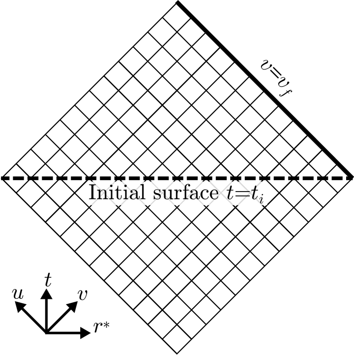
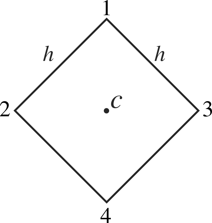
Figure 1: Left: Schematic picture of the numerical domain in the double null coordinates, $(u=t-r^{*},\,v=t+r^{*})$. We impose the close-limit, PN initial condition in Eqs. (17) and (18) on the surface with $t=t_{i}$ (the bold dashed line) and extract the waveform on the surface with $v=v_{f}$ (the bold solid line). Right: a cell in the numerical domain with the size of $h\times h$, where $h$ is the resolution and $C$ denotes the center of the cell.

To evolve Eq. (20), we use the finite-difference scheme developed by Lousto and Price Lousto and Price (1997). We introduce an uniform null grid in the $1+1$ numerical domain as the left panel of Figure 1. Consider a grid cell with the size of $h\times h$ in the domain. Integrating Eq. (20) over the cell gives

$$\Psi_{1}-\Psi_{2}-\Psi_{3}+\Psi_{4}+\frac{h^{2}}{8}V_{\ell}^{\textrm{Z}}(r_{c})(\Psi_{2}+\Psi_{3})+O(h^{4})=0\,,$$ (22)

where $r_{c}$ is the value of $r$ at the center of the cell, and $\Psi_{i}$ for $i=1,\,2,\,3,\,4$ correspond to the values of $\Psi$ (we have omitted the indices $(\ell,\,m)$ here) at the vertices of the cell in the right panel of Figure 1. By using the above equation, we can obtain $\Psi_{1}$ from $\Psi_{2}$, $\Psi_{3}$ and $\Psi_{4}$ with the local error term of $O(h^{4})$,

$$\Psi_{1}=\Psi_{2}+\Psi_{3}-\Psi_{4}-\frac{h^{2}}{8}V_{\ell}^{\textrm{Z}}(r_{c})(\Psi_{2}+\Psi_{3})+O(h^{4})\,.$$ (23)

The local error is accumulated through the integration over $v$ and $u$ to give a global error of $O(h^{2})$.

The finite-difference scheme on the initial surface should be derived separately. To implement the time-symmetric initial conditions in Eqs. (17) and (18), we also assume the time symmetry on the initial surface, and therefore $\partial_{t}\Psi|_{t=t_{0}}=0$, which leads to

$$\Psi_{1}=\Psi_{4}+O(h^{3})\,,$$ (24)

if the vertices 2 and 3 are on the surface. From this relation, we find that the finite-difference scheme on the initial surface is

$$\Psi_{1}=\frac{\Psi_{2}+\Psi_{3}}{2}-\frac{h^{2}}{16}V_{\ell}^{\textrm{Z}}(r_{c})(\Psi_{2}+\Psi_{3})+O(h^{3})\,.$$ (25)

While the local error term in this case is $O(h^{3})$, it eventually gives the global error of $O(h^{2})$ because the error is accumulated only over the initial surface. Hence, the convergence of our numerical solution through the finite difference scheme in Eqs. (23) and (25) is quadratic with respect to $h$ (see Figure 2 below).

3.3 Simulation parameters

In this paper, we calculate the Zerilli-Moncrief function with the close-limit, $2$PN initial data for head-on collisions of two nonspinning BHs in the following two cases:

• Case A: an equal mass collision with the initial separation of $r_{12}=3.5M$.

• Case B: an asymmetric mass collision with the mass ratio of $\nu=0.2$ and the initial separation of $r_{12}=4.4M$.

These system parameters are chosen so that they agree with those employed in Ref. Le Tiec and Blanchet (2010). In the case A, we focus only on $(\ell=2,\,m=0)$ mode because $(\ell=2,\,m=\pm 2)$ modes are just proportional to this mode. Similarly, in the case B, we look at only $(\ell=3,\,m=1)$ modes because $(\ell=3,\,m=-1)$ differs by only an overall minus sign, and $(\ell=3,\,m=\pm 3)$ modes are proportional to that mode; recall Eqs. (17) and (18).

3.4 Code validation

In our numerical simulations, the initial data given in Section 3.1 with the parameters shown in Section 3.3 is set on the region of $-1000\leq r^{*}/M\leq 3000$ at $t=t_{i}=0$ and the Zerilli equation in Eq. (20) are integrated within the future domain of dependence of the initial surface (the upper triangular domain in the left panel of Figure 1). The produced gravitational waveform is extracted on $v=v_{f}=3000M$ as a function of the retarded time $u=t-r^{*}$. We take the resolution as $h/M=(0.08,\,0.04,\,0.02,\,0.01,\,0.005)$ with the number of grid-point $N=(50000,\,100000,\,200000,\,400000,\,800000)$ respectively. From this point onward, we may set $M=1$.

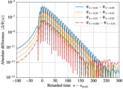
Figure 2: Absolute differences between the results with different resolutions, $h/M=(0.08,\,0.04,\,0.02,\,0.01,\,0.005)$. For example, $\Psi_{h=0.04}-\Psi_{h=0.08}$ (the blue solid curve) denotes the absolute differences between $(\ell=2,\,m=0)$ mode of the Zerilli-Moncrief function for the case A in the $h/M=0.08$ and $0.04$ simulations. The plot demonstrates the second order convergence of our time domain code. The numerical accuracy with the highest resolution is roughly estimated as $10^{-7}$ at the time of the peak amplitude $u_{\rm peak}$ and $10^{-13}$ in the late time of $(u-u_{\rm peak})/M\gtrsim 200$.

To check the convergence of our TD code, we consider the absolute differences between the Zerilli-Moncrief function $\Psi$ (we have omitted the indices $(\ell,\,m)$ here) computed with different resolutions,

$$\Delta\Psi=\left|\Psi_{h_{2}}-\Psi_{h_{1}}\right|\,,$$ (26)

where $h_{1}$ and $h_{2}$ denote adjacent resolutions. The result for the $(\ell=2,\,m=0)$ Zerilli-Moncrief function for the case A is shown in Figure 2. We can find that the difference becomes a quarter when the resolution gets a half. This shows the $O(h^{2})$ convergence of the data, as expected. The numerical accuracy with the highest resolution, $h=0.005M$, is roughly estimated as $10^{-7}$ at the time of the peak amplitude. In the late time of $(u-u_{\rm peak})/M\gtrsim 200$, the numerical accuracy becomes $10^{-13}$.

4 Modeling of ringdown waveforms

In this section, we introduce waveform models to describe the ringdown data in our close-limit calculations, as a superposition of QNMs associated with the remnant Schwarzschild BH. The method to compute QNMs are well developed in literature (see, e.g., Ref. Ringdown ). We use the accurate numerical data of QNM frequencies of the remnant BH provided by Berti Ringdown (for $\ell=2$) and those generated with the Black Hole Perturbation Club (B.H.P.C.) code Black Hole Perturbation Club (2020) (for $\ell=3$).

We should note that the zero-spin remnant BH here is a limitation of our close-limit approximation to the binary nonspinning BHs. When we treat general binary BH mergers in the full NR simulations with an astrophysically realistic initial data, the remnant BHs after merger are Kerr with a non-zero spin in general. For example, a nonspinning equal-mass binary BH of the quasicircular merger can produce a remnant Kerr BH with the nondimensional spin $\sim 0.67$ Lousto et al. (2010).

4.1 Standard quasinormal-mode fitting formula

We write the ringdown waveforms as a sum of the fundamental tone and overtones of QNMs decomposed into spin-weighted spherical harmonics with angular indices $(\ell,\,m)$ and spin $s=-2$, ${}_{-2}Y_{\ell m}(\theta,\varphi)$:

$$h=h_{+}-ih_{\times}=\frac{1}{r}\sum_{\ell,m}h_{N}^{\ell m}(t){}_{-2}Y_{\ell m}(\theta,\varphi)\quad(t\geq t_{0})\,,$$ (27)

with

$$h_{N}^{\ell m}(t)=\sum_{n=0}^{N}Q_{n}^{\ell m}e^{-i\omega_{\ell mn}^{\rm QNM}(t-t_{0})}\,,$$ (28)

where we truncate the summation with a finite overtone index of $n=N$ although there are infinite overtones. Here, $Q_{n}^{\ell m}$ is a complex amplitude, $\omega_{\ell mn}^{\rm QNM}$ is the Schwarzschild QNM frequency of the $(\ell,\,m,\,n)$ mode, and $t_{0}$ is the ’starting time’ before which we do not include the model to fit our numerical waveforms. As mentioned later, we choose the time of the peak amplitude of the wave, $t_{\textrm{peak}}$, as $t_{0}$.

With an appropriate choice of the initial phase, our numerical waveforms of the head-on collisions are given as purely real functions of the retarded time, $u$. Therefore, instead of the complex representation of the waveform in Eq. (28), we adopt the following real expression for the Zerilli-Moncrief function in practice, making use of the relation in Eq. (19),

$$\Psi_{N}^{\ell m}(u)=\sum_{n=0}^{N}\left[C_{2n}^{\ell m}\,\phi_{2n}^{\ell m}(u)+C_{2n+1}^{\ell m}\,\phi_{2n+1}^{\ell m}(u)\right]\,,$$ (29)

with

$$\phi_{2n}^{\ell m}(u) =\sqrt{\frac{4(\omega_{\ell mn}^{2}\tau_{\ell mn}^{2}+1)}{\omega_{\ell mn}^{2}\tau_{\ell mn}^{3}}}\,e^{-(u-u_{0})/\tau_{\ell mn}}\sin\left[\omega_{\ell mn}(u-u_{0})\right]\,,$$ (30)

$$\phi_{2n+1}^{\ell m}(u) =\sqrt{\frac{4(\omega_{\ell mn}^{2}\tau_{\ell mn}^{2}+1)}{(\omega_{\ell mn}^{2}\tau_{\ell mn}^{2}+2)\tau_{\ell mn}}}\,e^{-(u-u_{0})/\tau_{\ell mn}}\cos\left[\omega_{\ell mn}(u-u_{0})\right]\,,$$ (31)

where $C_{k}^{\ell m}$ ($k=0,\cdots,2N+1$) are real constants, $u_{0}$ is the starting time in terms of the retarded time, $\omega_{\ell mn}$ and $\tau_{\ell mn}$ are derived from the real and imaginary parts of the QNM frequency, respectively,

$$\omega_{\ell mn}=\Re(\omega_{\ell mn}^{\rm QNM})\,,$$ (32)

$$\tau_{\ell mn}=-\dfrac{1}{\Im(\omega_{\ell mn}^{\rm QNM})}\,.$$ (33)

The prefactor in the mode functions $\phi_{k}^{\ell m}(u)$ of Eqs. (30) and (31) is chosen so that they are certainly normalized (see the next subsection). We note that the model in Eq. (29) is a linear function with respect to the fitting coefficients $C_{k}^{\ell m}$. This means that one can obtain the best fit values of $C_{k}^{\ell m}$ through linear least squares.

4.2 Modified quasinormal-mode fitting formula with an orthonormal set of mode functions

The mode functions $\phi_{k}^{\ell m}(u)$ defined in the previous subsection are linearly independent but not orthogonal each other. For convenience of our analysis, we introduce an ‘orthonormal set’ of mode functions by using the Gram-Schmidt procedure. For this purpose, we first define the inner product between two real functions of $f(u)$ and $g(u)$ given in $u\geq u_{0}$

$$(f,\,g)\equiv\int_{u_{0}}^{\infty}f(u)g(u)\,du\,.$$ (34)

For this definition, we can find that $\phi_{k}^{\ell m}$ in Eqs. (30) and (31) is normalized as $(\phi_{k}^{\ell m},\,\phi_{k}^{\ell m})=1$.

Using the inner product in Eq. (34) and the standard Gram–Schmidt procedure, we obtain the orthonormal set of mode functions $\tilde{\phi}_{k}^{\ell m}$. Their explicit listing is

$$\tilde{\phi}_{0}^{\ell m} \equiv \phi_{0}^{\ell m}\,,$$ (35)

$$\tilde{\phi}_{1}^{\ell m} \equiv \frac{1}{\sqrt{1-(\tilde{\phi}_{0}^{\ell m},\,\phi_{1}^{\ell m})^{2}}}\left[\phi_{1}^{\ell m}-(\tilde{\phi}_{0}^{\ell m},\,\phi_{1}^{\ell m})\,\tilde{\phi}_{0}^{\ell m}\right]\,,$$ (36)

$$\tilde{\phi}_{2}^{\ell m} \equiv \frac{1}{\sqrt{1-(\tilde{\phi}_{1}^{\ell m},\,\phi_{2}^{\ell m})^{2}-(\tilde{\phi}_{0}^{\ell m},\,\phi_{1}^{\ell m})^{2}}}$$ (38)

$$\times\left[\phi_{2}^{\ell m}-(\tilde{\phi}_{1}^{\ell m},\,\phi_{2}^{\ell m})\,\tilde{\phi}_{1}^{\ell m}-(\tilde{\phi}_{0}^{\ell m},\,\phi_{2}^{\ell m})\,\tilde{\phi}_{0}^{\ell m}\right]\,,$$

$$\tilde{\phi}_{3}^{\ell m} \equiv \frac{1}{\sqrt{1-(\tilde{\phi}_{2}^{\ell m},\,\phi_{3}^{\ell m})^{2}-(\tilde{\phi}_{1}^{\ell m},\,\phi_{3}^{\ell m})^{2}-(\tilde{\phi}_{0}^{\ell m},\,\phi_{3}^{\ell m})^{2}}}$$ (40)

$$\times\left[\phi_{3}^{\ell m}-(\tilde{\phi}_{2}^{\ell m},\,\phi_{3}^{\ell m})\,\tilde{\phi}_{2}^{\ell m}-(\tilde{\phi}_{1}^{\ell m},\,\phi_{3}^{\ell m})\,\tilde{\phi}_{1}^{\ell m}-(\tilde{\phi}_{0}^{\ell m},\,\phi_{3}^{\ell m})\,\tilde{\phi}_{0}^{\ell m}\right]\,,$$

$$\vdots$$ (41)

$$\tilde{\phi}_{k}^{\ell m} \equiv \left[1-\sum_{p=0}^{k-1}(\tilde{\phi}_{p}^{\ell m},\phi_{k}^{\ell m})^{2}\right]^{-1/2}\left[\phi_{k}^{\ell m}-\sum_{p=0}^{k-1}(\tilde{\phi}_{p}^{\ell m},\phi_{k}^{\ell m})\,\tilde{\phi}_{p}^{\ell m}\right]\,.$$ (42)

However, we note that a direct numerical implementation of above construction does not work well because of the accumulation of round-off errors. In practice, we use the modified Gram-Schmidt algorithm Golub and Van Loan (1996) to obtain accurately the orthonormal set of mode functions.

From the above orthonormal set of mode functions $\tilde{\phi}_{k}^{\ell m}$, we can extract the fitting coefficients easily by

$$\tilde{C}_{k}^{\ell m}=(\tilde{\phi}_{k}^{\ell m},\,\Psi^{\ell m}_{\rm num})\,,$$ (43)

from the numerically generated Zerilli-Moncrief function $\Psi^{\ell m}_{\rm num}$, and construct the modified model waveform as

$$\tilde{\Psi}_{N}^{\ell m}(u)=\sum_{k=0}^{2N+1}\tilde{C}_{k}^{\ell m}\tilde{\phi}_{k}^{\ell m}(u)\,,$$ (44)

up to a finite overtone index of $n=N$.

5 Results

We now present the demonstration of the QNM fits including overtones given in Eqs. (29) and (44) with the close-limit TD waveform for head-on collisions explained in Section 3.

5.1 Quasinormal-mode fitting and residuals

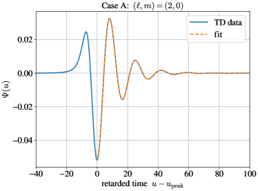
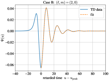
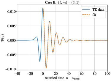
Figure 3: TD data of the Zerilli-Moncrief functions $\Psi^{\ell m}$ with the 2PN close-limit initial data for the head-on collision (the blue solid lines) and QNM fitting with $N=7$ in Eq. (44) (the orange dashed lines). The TD data is extracted as a function of the retarded time, $u$ on the $v=v_{f}=3000M$ surface. The top panel shows the $(\ell=2,\,m=0)$ mode computed for the case A. The bottom two panel shows the $(\ell=2,\,m=0)$ mode (left) and the $(\ell=3,\,m=1)$ mode (right) computed for the case B.

Figure 3 shows the QNM fit including overtones in Eq. (44) to the $(\ell=2,\,m=0)$ mode of the Zerilli-Moncrief function $\Psi^{\ell m}$ in the case A (top). Similarly, in the case B, we show the QNM fits to the $(\ell=2,\,m=0)$ mode (bottom-left) and to the $(\ell=3,\,m=1)$ mode (bottom-right), respectively. In each panel, the QNM overtone in the model waveform is truncated at $N=7$ and the time of the peak amplitude, $u_{\textrm{peak}}$ is chosen as the starting time, $u_{0}$.

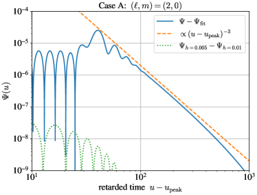
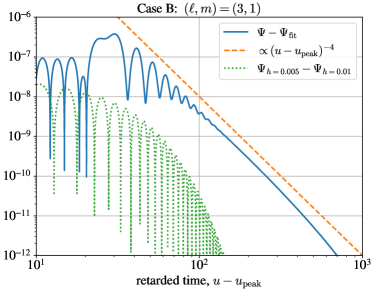
Figure 4: Fit residuals (the blue solid lines) between the Zerilli-Moncrief TD data $\Psi^{\ell m}_{\rm num}$ and the QNM fit including overtones with $N=7$. The grouping of panels are the same as for Figure 3. For reference, we plot $\Delta\Psi$ in Eq. (26) with $h_{1}=0.01M$ and $h_{2}=0.005M$ (the green dotted lines) to roughly estimates the numerical error in the data. We also show the lines proportional to $(u-u_{\textrm{peak}})^{-3}$ in the top and bottom-left panel and to $(u-u_{\textrm{peak}})^{-4}$ in the bottom-right panel in order to see the late-time behavior (the orange dashed lines).

Figure 4 provides the QNM fit residuals of Figure 3 (the blue solid lines). We find that the residuals are all larger than our numerical uncertainty (the green dotted lines), and shows the power-law behavior in the late time ($u-u_{\textrm{peak}}>100M$, the orange dashed lines). This corresponds to the late-time tail in the evolution of a perturbation of the gravitational field around a remnant Schwarzschild BH, studied in various literature; see, e.g., Refs. Leaver (1986); Ching et al. (1995); Andersson (1997) for the Schwarzschild background spacetime, and, e.g., Refs. Krivan et al. (1997); Pazos-Avalos and Lousto (2005) for the Kerr background spacetime. The power-law tail in a sufficiently late time is also investigated using a sophisticated numerical method with compactification along hyperboloidal surfaces Zenginoglu et al. (2009). Each of QNM fit residuals deviates from the power-law line when $u$ becomes larger because the null infinity approximation $v\gg u$ is broken (see Section IV in Ref. Gundlach et al. (1994)).

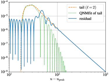
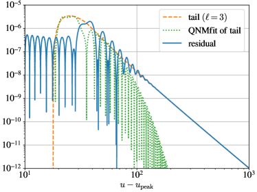
Figure 5: Analysis of mock data of the tail component in Eq. (45) (the orange dashed lines). We plot the $(\ell=2)$ and $(\ell=3)$ modes in the left and right panels, respectively. The green dotted lines show the QNM fit including overtones with $N=7$ and the blue solid lines are the fit residuals. Here, we choose $D_{l}=1$, $u_{1}=u_{\textrm{peak}}+10M$ and $u_{2}=u_{\textrm{peak}}+30M$ in Eq. (45) with Eq. (46).

In Figure 4, we also find that the QNM fit residuals in the early-time ($u-u_{\textrm{peak}}\lesssim 100M$) do not improve even if one includes more overtones into the model waveform in Eq. (44). Although we do not have a mathematically rigorous proof, we speculate that this limitation may arise from the QNM fit including overtones (that describes the exponential decay of the perturbation) to the power-law tail component of the perturbation, based on a simple numerical experiment detailed below.

First, we prepare a mock data of the tail component of the perturbation as

$$\Psi^{\ell m}_{\textrm{tail}}(u)=D_{\ell}W(u)\left(\frac{u-u_{\textrm{peak}}}{M}\right)^{-\ell-1}\,,$$ (45)

where $D_{\ell}$ is an arbitrary constant, and we define a window function by

$$W(u)=\left\{\begin{array}[]{ll}0&(u<u_{1})\,,\\ \dfrac{(u-u_{1})^{2}(2u+u_{1}-3u_{2})}{(u_{1}-u_{2})^{3}}&(u_{1}\leq u\leq u_{2})\,,\\ 1&(u_{2}<u)\,,\end{array}\right.$$ (46)

with $u_{\textrm{peak}}<u_{1}<u_{2}$. The window function is introduced to remove the divergent behavior of the late-time tail at $u=u_{\textrm{peak}}$.

Next, we fit this mock data using the QNM model including overtones in Eq. (44) in the same manner as we do for the TD data. Figure 5 shows the QNM fit including overtones to the mock tail data and corresponding fit residuals. We see that the residuals in the early-time ($(u-u_{\textrm{peak}})/M\lesssim 100$) show the similar behaviour in Figure 4. This result supports our expectation about the early-time residual in the TD data.

5.2 Convergence of the fitting coefficients

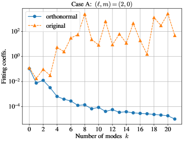
Figure 6: Left: the absolute values of the fitting coefficients, $\tilde{C}_{k}^{\ell m}$ (the blue filled circles) and $C_{k}^{\ell m}$ (the orange filled triangles) for the $(\ell=2,\,m=0)$ mode in the case A, as a function of mode $k$. $\tilde{C}_{k}^{\ell m}$ is calculated by Eq. (43), while $C_{k}^{\ell m}$ is obtained by the least square fit of the TD data to the model in Eq. (29). Right: the estimator $\Delta_{n}$ in Eq. (48) as a function of overtones $n$.

Because the model waveform in Eqs. (29) and (44) involves many overtones $k$ (or $N$) it is instructive to check their convergence in terms of fitting coefficients on $k$, to ask how higher overtones should be included in practice when we wish to model the TD data from the peak time at $u=u_{\textrm{peak}}$.

In the left panel of Figure 6 where the TD data is for the $(\ell=2,\,m=0)$ mode in the case A, we show the fitting coefficients for the original QNM basis $C_{k}^{\ell m}$ (the orange filled triangles) and those for the orthonormal set of mode functions $\tilde{C}_{k}^{\ell m}$ (the blue filled circles) as a function of overtones up to $k\leq 21$ (i.e., $N=10$). It is found that $|\tilde{C}_{k}^{\ell m}|$ decreases roughly in power law of $k$, while $|C_{k}^{\ell m}|$ does not.

Due to the benefit of the orthonormalization of mode functions in Eq. (44), it can be conveniently used to assess the fraction of power in each mode

$$\rho^{2}\equiv(\tilde{\Psi}_{N}^{\ell m},\tilde{\Psi}_{N}^{\ell m})=\sum_{k=0}^{2N+1}|\tilde{C}_{k}^{\ell m}|^{2}\,.$$ (47)

Based on the fact that one more mode is added to the orthonormal set when $k$ increases by two, we introduce an estimator to characterize the match (or overlap) between the TD data and the QNM fit model including overtones at a given $n$

$$\Delta_{n}\equiv\frac{\sqrt{|\tilde{C}_{2n}^{\ell m}|^{2}+|\tilde{C}_{2n+1}^{\ell m}|^{2}}}{\rho}\,.$$ (48)

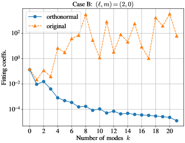
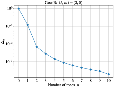
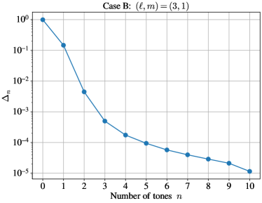
Figure 7: The same figure as for Figure 6, but using the $(\ell=2,\,m=0)$ mode (top) and $(\ell=3,\,m=1)$ mode (bottom) in the case B.

The right panel of Figure 6 shows $\Delta_{n}$ as a function of mode $n$. We see that the inclusion of the first overtone ($n=1$) can improve the match by $10\%$, and that the QNM fits up to $n=5$ will suppress the mismatch less than $0.1\%$.

In the top and bottom panels of Figure 7, we show the same figures as for Figure 6 but with the $(\ell=2,\,m=0)$ and $(\ell=3,\,m=1)$ modes in the case B, respectively. We see the similar convergent behavior in $\tilde{C}_{k}^{\ell m}$ here, and again find that $(n\geq 5)$ higher overtones contributes to the match only at the level of less than $0.1\%$. These results highlight the potential benefit to use the orthonormal set of mode functions in the data analysis of ringdown GWs.

6 Summary and Discussion

It is now widely recognized the importance to have a ringdown waveform model including higher overtones of QNMs (see, e.g., Ref. Giesler et al. (2019)). With the overtones, one can set the starting time of the ringdown GWs at the time of the peak amplitude much earlier than a time ($\sim 10M$ – $20M$ after the peak time) to obtain unbiased remnant BH parameters (see, e.g., Figure 5 for GW150914 in Ref. Abbott et al. (2016b)). This allows the increased SNR of observed ringdown signals as well as better parameter estimation of the remnant BH.

In this paper, we examined in detail the ringdown GWs of binary BHs with QNM fits including overtones in Eqs. (29) and (44), using the accurate close-limit waveform in the BH perturbation theory as a test bed. Our analysis is restricted to the narrow case of head-on collisions of two nonspinning BHs (based on the $2$PN initial data and linear BH perturbation theory), but it suffices to highlight some of the key features of the full problem, and we found three main results: (i) we reconfirm the importance of QNMs overtones to fit the ringdown waveforms after the time of the peak amplitude. This agrees with the previous findings in literature Giesler et al. (2019); Mourier et al. (2021); (ii) the small contributions of late-time tail exist in the fit residuals at the level of $O(10^{-5})$ or below (see Figure 4); (iii) the fitting coefficients decay with overtones when one uses the orthonormal set of mode functions in Eq. (43) (see Figures 6 and 7).

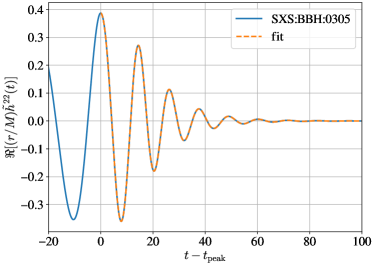
Figure 8: Left: the $(\ell=2,\,m=2)$ spheroidal harmonic mode of the NR waveform SXS:BBH:0305 (the blue solid line) and the QNM fit including overtone with orthonormalized mode functions introduced in Eq. (44) (the orange dashed line). Right: the NR data (the blue solid line) and the fit residuals (the orange dashed line).

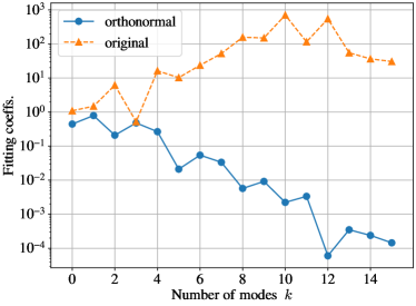
Figure 9: Fitting coefficients of the $(\ell=2,\,m=2)$ spheroidal harmonic mode of SXS:BBH:0305. The left panel displays the absolute values of the fitting coefficients for $\tilde{C}_{k}^{\ell m}$ (the blue filled circles) and $C_{k}^{\ell m}$ (the orange filled triangles). The plots in the right column shows $\Delta_{n}$ in Eq. (48).

A natural next step of our study is to assess the merit of the orthonormal set of mode functions in the context of GW data analysis, accounting for the detector’s noise. A standard technique for the analysis of ringdown GWs is the frequency-domain approach (see, e.g., Ref. Nakano et al. (2019) for various methods to extract the ringdown GWs), and we can directly apply the orthonormal set of mode function presented in Section 4.2 with the (so named) noise-weighted inner product in the matched filtering method (see, e.g., Ref. Uchikata et al. (2020)). The implementation of this method to the GW data analysis and the analysis of real data from GW detectors will be a future work.

Another interesting future work would be to add BH’s spin to our close-limit waveform. Although it is known for any field points that the $2.5$PN near-zone metric with spin effects Tagoshi et al. (2001); Faye et al. (2006), the numerical computation of either metric or curvature perturbations in Kerr spacetime is particularly challenging in the time domain Sundararajan et al. (2007); Dolan and Barack (2013); Long and Barack (2021), and would need much coding efforts. It is probably more viable, instead, to perturbatively include the spin effect into our non-spinning close-limit waveform (e.g., Lousto et al. (2010)). It may be also possible to calculate the close-limit waveform in Kerr case making use of the standard frequency-domain technique (and taking the extreme mass-ratio limit). Because, in either case, the extension is involved, we leave them for future work.

From the theoretical point of view, it will be useful to include information on excitation coefficients and factors for the fundamental tone and overtones of QNMs derived from the BH perturbation approach (See, e.g., Refs. Berti and Cardoso (2006); Zhang et al. (2013); Hughes et al. (2019); Lim et al. (2019)). Also, although we focused only on the $(\ell=2,\,m=0)$ and $(\ell=3,\,m=1)$ modes in the bulk of this paper (and will focus only on the $(\ell=2,\,m=2)$ mode in Appendix A), the inclusion of the other subdominant (higher harmonic) modes will be beneficial. In particular, the $(\ell=4,\,m=4)$ mode of NR waveforms for binary BHs is especially interesting because this mode includes the second order modes composed by the non-linear, self-coupling of first-order $(\ell=2,\,m=2)\times(\ell=2,\,m=2)$ mode, and it has already been found in NR simulations London et al. (2014).

Nevertheless, astute readers may ask what extent the results based on the close-limit approximation (to the head-on collisions of two nonspinning BHs) are consistent with the full NR waveforms in more astrophysically relevant scenarios (e.g., coalescences observed by LIGO/Virgo). We conclude our paper to briefly answer this question, analyzing the NR waveform of SXS:BBH:0305 in the Simulating eXtreme Spacetimes (SXS) catalogue SXS Gravitational Waveform Database with the same approach that we took in Section 5; Appendices A and B also provide supplemented examples of the analysis for NR waveforms.

Figure 8 shows the $(\ell=2,\,m=2)$ spheroidal mode of the waveform SXS:BBH:0305 Lovelace et al. (2016); Boyle et al. (2019); SXS Gravitational Waveform Database (see Eq. (49) for the construction of the spheroidal modes from the spherical ones). Here, we set the time of the peak amplitude as the starting time of the QNM fit (see the orange dashed line in the left panel of Figure 8), and we use the QNM fitting formula introduced in Eq. (44). Unlike the TD data generated within the close-limit approximation and the BH perturbation approach, we cannot confirm the power-law tail certainty due to some constant fit residuals of $\sim 10^{-5}$ after $t-t_{\textrm{peak}}\gtrsim 80M$; recall that the tail contribution in Figure 4 is at the level of $\lesssim O(10^{-5})$, which is as large as the remaining residual in the NR waveform. We expect that future NR simulation with higher numerical accuracy (or, e.g., the close-limit approximation to bound-orbit BBH mergers) will provide a more robust answers of the need of the tail contribution in the ringdown waveform modeling, and eventually in the measurement of remnant properties of BHs.

Figure 9 displays the fitting coefficients for the original QNM basis $C_{k}^{\ell m}$ and those for the orthonormalized QNM basis $\tilde{C}_{k}^{\ell m}$ introduced in Eq. (43), again focusing on the the $(\ell=2,\,m=2)$ spheroidal mode of SXS:BBH:0305. We see that the trend of $C_{k}^{\ell m}$ and $\tilde{C}_{k}^{\ell m}$ are similar to that of the close-limit, TD data displayed in Figures 6 and 7 (see also Appendix B). Namely, $\tilde{C}_{k}^{\ell m}$ converges as increasing the overtone $k$ while $C_{k}^{\ell m}$ (from the least square fit by using Eq. (29)) does not. The convergence property of $\tilde{C}_{k}^{\ell m}$ supports the argument that the dominant $(\ell=2,\,m=2)$ mode of NR waveforms after the time of the peak amplitude can be described only by the QNMs in the linearized BH perturbation (see Section 1 for the other confirmations).

The authors contribute equally to this paper.

N. S. and H. N. acknowledge support from JSPS KAKENHI Grant No. JP21H01082 and No. JP17H06358. S. I. acknowledges support from STFC through Grant No. ST/R00045X/1. S. I. also thanks to networking support by the GWverse COST Action CA16104, “Black holes, gravitational waves and fundamental physics.” H. N. acknowledges support from JSPS KAKENHI Grant No. JP21K03582.

Appendix A Analysis of some numerical-relativity waveforms in time domain

In this appendix and Appendix B, we focus on the $(\ell=2,\,m=2)$ (spheroidal harmonic) mode of the ringdown signal (after the time of the peak amplitude) provided by NR waveforms for nonprecessing, spinning binary BH mergers, and analyze them following the same approach as in Section 5. Our goal here is to examine if we find i) the late-time, power-law tail (this appendix) and ii) the convergence of the orthonormalized QNM fits (Appendix B) in more astrophysically relevant NR waveforms. We note that there are also various works on the mismatch and parameter estimation errors based on the ringdown portion of the NR waveforms and their QNM fits with overtones Giesler et al. (2019); Bhagwat et al. (2020); Ota and Chirenti (2020); Cook (2020); Jiménez Forteza et al. (2020); Jiménez Forteza and Mourier (2021), memory (mainly the $m=0$ mode) Mitman et al. (2020) and mirror (negative $m$) modes Dhani (2021); Dhani and Sathyaprakash (2021).

Table 1: Masses and spins of remnant BHs from NR simulations of binary BHs examined in this Appendix. $M_{\rm rem}/M$ and $\chi_{\rm rem}$ are the nondimensional mass ans spin parameters, respectively. The ‘SXS’ data is presented in the Simulating eXtreme Spacetimes (SXS) catalogue SXS Gravitational Waveform Database while the ‘RIT’ data is imported from the CCRG@RIT Catalog of Numerical Simulations CCRG@RIT Catalog of Numerical Simulations . Each reference in the table is cited from the corresponding metadata file. SXS:BBH:0305 is used in Section 6, and the remaining NR data are studied in Appendices A and B.

ID	Mass ($M_{\rm rem}/M$)	Spin ($\chi_{\rm rem}$)	Reference
SXS:BBH:0305	0.952032939704	0.6920851868180025	Lovelace et al. (2016); Boyle et al. (2019); SXS Gravitational Waveform Database
SXS:BBH:1936	0.9851822160611967	0.021659378750190413	Varma et al. (2019); Boyle et al. (2019); SXS Gravitational Waveform Database
SXS:BBH:0260	0.9810057011067479	0.12447236057508855	Chu et al. (2016); Boyle et al. (2019); SXS Gravitational Waveform Database
SXS:BBH:1501	0.93633431069	0.8085731624240002	Varma et al. (2019); Boyle et al. (2019); SXS Gravitational Waveform Database
SXS:BBH:1477	0.911077401717	0.907542632208	Varma et al. (2019); Boyle et al. (2019); SXS Gravitational Waveform Database
SXS:BBH:0178	0.8866898235070239	0.9499311295284206	Scheel et al. (2015); Boyle et al. (2019); SXS Gravitational Waveform Database
SXS:BBH:1124	0.8827804590335694	0.9506671398803149	Boyle et al. (2019); SXS Gravitational Waveform Database
RIT:BBH:0062	0.9520211506	0.6919694604	Healy et al. (2017, 2019); Healy and Lousto (2020)
RIT:BBH:0604	0.9361520656	0.8101416903	Healy et al. (2017, 2019); Healy and Lousto (2020)
RIT:BBH:0558	0.9108618514	0.9077062488	Healy et al. (2017, 2019); Healy and Lousto (2020)
RIT:BBH:0767	0.9057246958	0.9462438132	Healy et al. (2017, 2019); Healy and Lousto (2020)

In our analysis of the NR waveforms, we fix the values of remnant BH mass $M_{\textrm{rem}}/M$ and spin $\chi_{\textrm{rem}}$ provided by the NR simulations (see Table 1) and calculate the QNM frequencies by assuming a Kerr geometry with these remnant properties. We also mean the $(\ell=2,\,m=2)$ mode as that in terms of the spin-weighted spheroidal harmonics. Because the NR waveforms rather adopt the spherical basis, we have to account for the mixing of spheroidal and spherical bases here. The GW strain is decomposed in terms of the spherical and spheroidal harmonics as

$$h= \frac{1}{r}\sum_{\ell,\,m}h^{\ell m}(t){}_{-2}P_{\ell m}(\theta)\frac{e^{im\varphi}}{\sqrt{2\pi}}$$ (49)

$$= \frac{1}{r}\sum_{\ell^{\prime},\,m}\tilde{h}^{\ell^{\prime}m}(t){}_{-2}S_{\ell^{\prime}m}^{a\omega}(\theta)\frac{e^{im\varphi}}{\sqrt{2\pi}}\,,$$ (50)

where ${}_{-2}P_{\ell m}(\theta)$ and ${}_{-2}S_{\ell m}^{a\omega}(\theta)$ are the spin-weighted associated Legendre function and the spin-weighted spheroidal harmonics, respectively. When calculating the $(\ell=2,\,m=2)$ spheroidal harmonic mode, we take into account the mixing of $2\leq\ell\leq 8$ (for the SXS data) and $2\leq\ell\leq 4$ (for the RIT data) spherical harmonic modes by using the relation as

$$\tilde{h}^{\ell^{\prime}m}(t)=\int_{0}^{\pi}d\theta\,\sin\theta\,\sum_{\ell}h^{\ell m}(t){}_{-2}P_{\ell m}(\theta){}_{-2}S_{\ell^{\prime}m}^{a\omega}(\theta)\,.$$ (51)

Figure 10: Real part of the $(\ell=2,\,m=2)$ spheroidal harmonic mode $\Re(\tilde{h}^{22})$ of SXS NR waveforms listed in Table 1 and their QNM fit residuals. Each plot corresponds to that in the right panel of Figure 8 in the case of SXS:BBH:0305.

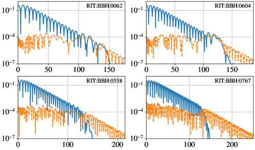
Figure 11: Real part of the $(\ell=2,\,m=2)$ spheroidal harmonic mode $\Re(\tilde{h}^{22})$ of RIT NR waveforms listed in Table 1 and their QNM fit residuals.

Figure 10 shows the QNM fit residuals of the $(\ell=2,\,m=2)$ SXS ringdown waveforms: SXS:BBH:1936 (almost nonspinning remnant BH, $\chi_{\rm rem}\sim 0.02$) Varma et al. (2019); Boyle et al. (2019); SXS Gravitational Waveform Database , SXS:BBH:0260 (slowly rotating remnant BH, $\chi_{\rm rem}\sim 0.12$) Chu et al. (2016); Boyle et al. (2019); SXS Gravitational Waveform Database , SXS:BBH:1501 (spinning remnant BH, $\chi_{\rm rem}\sim 0.81$) Varma et al. (2019); Boyle et al. (2019); SXS Gravitational Waveform Database , SXS:BBH:1477 (spinning remnant BH, $\chi_{\rm rem}\sim 0.91$) Varma et al. (2019); Boyle et al. (2019); SXS Gravitational Waveform Database , SXS:BBH:0178 (highly spinning remnant BH, $\chi_{\rm rem}\sim 0.95$) Scheel et al. (2015); Boyle et al. (2019); SXS Gravitational Waveform Database , and SXS:BBH:1124 (highly spinning remnant BH, $\chi_{\rm rem}\sim 0.95$) Boyle et al. (2019); SXS Gravitational Waveform Database . Here, we use only $\Re(\tilde{h}^{\ell m})$ from Eq. (51) of the NR waveforms and apply the real expression for the QNM fit model in Eq. (44) with overtones up to $N=7$ (by replacing $\Psi^{\ell m}$ with $\Re(\tilde{h}^{\ell m})$ and accounting for the orthonormalization of QNM basis in Section 4.2).

We find that all the SXS waveform data in the late time have the same constant residue of $O(10^{-5})$ as for SXS:BBH:0305, except for BBH:1477 that has the shorter time stretch between the peak and the end of data including the original data than other data set. We cannot identify the late-time tails in the QNM fit residuals (at least) in these NR waveforms, and some improvement in accuracy of NR simulation may be needed in order to reveal the tails.

We also find the slower damping fit residuals than the $(\ell=2,\,m=2)$ mode itself in the late-time part of SXS:BBH:0178 and SXS:BBH:1124 (with highly spinning remnant BHs, $\chi_{\textrm{rem}}\sim 0.95$). This is rather unexpected result because any QNMs (even including the second and higher order perturbations) have a faster damping time than the fundamental tone ($\ell=2,\,m=2,\,n=0$) in the high-spin range; see Figure 14 in Appendix C.

To have additional evidence for the above slower damping fit residuals, we examine another NR waveform set produced by RIT team Healy et al. (2017, 2019); Healy and Lousto (2020), including RIT:BBH:0062 (spinning remnant BH, $\chi_{\rm rem}\sim 0.69$), RIT:BBH:0604 (spinning remnant BH, $\chi_{\rm rem}\sim 0.81$), RIT:BBH:0558 (spinning remnant BH, $\chi_{\rm rem}\sim 0.91$), and RIT:BBH:0767 (highly spinning remnant BH, $\chi_{\rm rem}\sim 0.95$), and display their QNM fit residuals in Figure 11. RIT:BBH:0767 (bottom-right) has the remnant spin as high as that of SXS:BBH:0178 and SXS:BBH:1124, but we cannot confidently identify the similar slow-damping residuals due to the larger numerical error at $\sim 10^{-4}$. The source of this slower damping residuals remains unclear to us, and more systematic investigation awaits future work.

Before concluding this appendix, we should note the possible second-order contribution, i.e., the self-coupling of the two first-order QNMs computed from the linear perturbation theory, to our analysis. For example, the second-order, $(\ell=2,\,m=2)\times(\ell=2,\,m=2)$ mode is found in NR simulations London et al. (2014). This mode is corresponding to the second order $(\ell=4,\,m=4)$ mode, and we did not consider it here. Also, in principle, the $(\ell=2,\,m=2)$ mode include the second-order contribution like $(\ell=2,\,m=1)\times(\ell=2,\,m=1)$ mode, but we cannot find these second-order contributions in our analysis. This is consistent with the previous work in Ref. London et al. (2014).

Appendix B Analysis of the fitting coefficients of some numerical-relativity data

As a by-product of the analysis in Appendix A, we obtain the fitting coefficients (in terms of the original QNM basis and the orthonormal set of mode functions) for the NR data listed in Table 1, and can check the convergence in the same manner as shown in Figure 9. We summarize the results in Figure 12 for the SXS data and Figure 13 for the RIT data. From these results, we expect that the contribution from the overtones to the ringdown waveform becomes more significant with larger remnant spins. The further study will be required to clarify the relation between the parameters of binary BHs and the significance of the overtones (A comprehensive study of the dependence of the mode excitations on the source parameters has been done in the extreme mass-ratio limit Hughes et al. (2019); Lim et al. (2019)).

Figure 12: The waveforms and fitting coefficients of samples of SXS data listed in Table 1. The plots in the left column show the real part of $(\ell=2,\,m=2)$ spheroidal harmonic mode (the blue solid line) and the QNM fit to the model with the orthonormal set given in Eq. (44) (the orange dashed line). The plots in the center column present the absolute values of the fitting coefficients for $\tilde{C}_{k}^{\ell m}$ (the blue filled circles) and $C_{k}^{\ell m}$ (the orange filled triangles). The plots in the right column show $\Delta_{n}$ in Eq. (48).

Figure 13: The waveforms and fitting coefficients of samples of RIT data listed in Table 1. The plots in the left column show the real part of the $(\ell=2,\,m=2)$ spheroidal harmonic mode (the blue solid line) and the QNM fit to the model with the orthonormal set given in Eq. (44) (the orange dashed line). The plots in the center column present the absolute values of the fitting coefficients for $\tilde{C}_{k}^{\ell m}$ (the blue filled circles) and $C_{k}^{\ell m}$ (the orange filled triangles). The plots in the right column show $\Delta_{n}$ in Eq. (48).

Appendix C Frequencies of Kerr quasinormal modes

Although many plots for Kerr QNM frequencies are available in literature, e.g., in Refs. Onozawa (1997); Berti et al. (2009); Cook and Zalutskiy (2014), we reproduce a QNM figure here for $m=\ell$ modes using publicly available data provided in “Ringdown” by Berti Ringdown (see also “Kerr Quasinormal Modes: $s=-2$, $n=0$–$7$” by Cook Kerr Quasinormal Modes: $s=-2$, $n=0$-$7$ ). They give the lowest damping rate in each $\ell$ mode, and help to check the presence of the second order perturbation in our analysis. Below the indices $(\ell,\,m)$ refer to the spin-weighted spheroidal basis with $s=-2$.

Figure 14 shows the Kerr QNM frequencies (the fundamental tone and overtones up to $n=7$) for the nondimensional spin $0\leq\chi\leq 0.999$, but it suffices to consider the QNM frequencies up to the filled circles ($\chi=0.95$) because the NR simulations used for our study have the remnant BH spin $\chi\lesssim 0.95$ after merger. In particular, we see that the $(\ell=2,\,m=2,\,n=0)$ mode has the lowest damping rate (recall Eq. (33)). Importantly, the first order $(\ell=2,\,m=2,\,n=0)$ mode remains to be the longest-lived mode even when considering the second and higher order QNMs as we establish below.

Figure 14: Fundamental tone and overtones of Kerr QNMs for $m=\ell$ modes. Here $\omega_{R}$ and $\omega_{I}$ mean the real and imaginary parts of the QNM frequency, respectively. We plot the values for $2\leq\ell\leq 7$ in the range of the nondimensional spin of $0\leq\chi\leq 0.999$. The filled circles show the QNM values at $\chi=0.95$. For $\chi\leq 0.95$, the $n=0$ mode always has the highest real frequency and the slowest damping time. There is an interesting feature in the fifth overtone ($n=5$) of the $m=\ell=2$ mode. To make these plots, we use the QNM data provided in Ref. Ringdown .

Suppose an expansion of the metric of the form,

$$g_{\mu\nu}=g_{\mu\nu}^{(0)}+h_{\mu\nu}^{(1)}+h_{\mu\nu}^{(2)}+(\text{higher-order terms})\,,$$ (52)

where $g_{\mu\nu}^{(0)}$ is a background (Kerr) spacetime, and $h_{\mu\nu}^{(1)}$ is the first order perturbation here. The second order perturbation $h_{\mu\nu}^{(2)}$ formally satisfies the linearized Einstein equation

$$G_{\mu\nu}^{(1)}[h^{(2)}]=-G_{\mu\nu}^{(2)}[h^{(1)},\,h^{(1)}]\,,$$ (53)

where $G_{\mu\nu}^{(1)}$ is the linearized Einstein tensor (in a given gauge), and $G_{\mu\nu}^{(2)}[h^{(1)},\,h^{(1)}]$ is the term quadratic in $h^{(1)}$ in the expansion of the Einstein tensor. Although the real part of second-order QNM frequencies of $h_{\mu\nu}^{(2)}$ can take various values due to the self-mode coupling of $h_{\mu\nu}^{(1)}$ through $G_{\mu\nu}^{(2)}$, Figure 14 indicates that for $\chi\lesssim 0.95$ the imaginary part of any second-order QNM frequencies $\omega_{I}^{(2)}$ is bounded at Ioka and Nakano (2007); Nakano and Ioka (2007)

$$\left|\omega_{I}^{(2)}\right|\geq 2\,\left|\omega_{I,\,220}^{(1)}\right|\,,$$ (54)

where $\omega_{I,\,220}^{(1)}$ is the imaginary part of the first order $(\ell=2,\,m=2,\,n=0)$ QNM frequency. This in turn implies that the damping time of any second order QNMs satisfies

$$\tau^{(2)}\leq\frac{1}{2}\,\tau_{220}\,.$$ (55)

Therefore, the first order $(\ell=2,\,m=2,\,n=0)$ QNM has the slowest damping time, at least to the second order in the expansion of the metric and for $0\leq\chi\leq 0.95$ of the remnant BH (whose imaginary part of the first order QNMs is not too close to zero).

References

yes

References

- Kerr (1963) Kerr, R.P. Gravitational Field of a Spinning Mass as an Example of Algebraically Special Metrics. Phys. Rev. Lett. 1963, 11, 237–238. doi:\changeurlcolorblack10.1103/PhysRevLett.11.237.
- Abbott et al. (2021a) Abbott, R.; others. GWTC-2: Compact Binary Coalescences Observed by LIGO and Virgo During the First Half of the Third Observing Run. Phys. Rev. X 2021, 11, 021053, [arXiv:gr-qc/2010.14527]. doi:\changeurlcolorblack10.1103/PhysRevX.11.021053.
- Abbott et al. (2021b) Abbott, R.; others. GWTC-2.1: Deep Extended Catalog of Compact Binary Coalescences Observed by LIGO and Virgo During the First Half of the Third Observing Run. arXiv e-prints 2021, p. arXiv:2108.01045, [arXiv:gr-qc/2108.01045].
- Nakamura et al. (2016) Nakamura, T.; Nakano, H.; Tanaka, T. Detecting quasinormal modes of binary black hole mergers with second-generation gravitational-wave detectors. Phys. Rev. D 2016, 93, 044048, [arXiv:astro-ph.HE/1601.00356]. doi:\changeurlcolorblack10.1103/PhysRevD.93.044048.
- Nakamura and Nakano (2016) Nakamura, T.; Nakano, H. How close can we approach the event horizon of the Kerr black hole from the detection of gravitational quasinormal modes? PTEP 2016, 2016, 041E01, [arXiv:gr-qc/1602.02385]. doi:\changeurlcolorblack10.1093/ptep/ptw026.
- Nakano et al. (2016) Nakano, H.; Nakamura, T.; Tanaka, T. The detection of quasinormal mode with a/M = 0.95 would prove a sphere 99% soaking in the ergoregion of the Kerr space-time. PTEP 2016, 2016, 031E02, [arXiv:gr-qc/1602.02875]. doi:\changeurlcolorblack10.1093/ptep/ptw015.
- Nakano et al. (2015) Nakano, H.; Tanaka, T.; Nakamura, T. Possible golden events for ringdown gravitational waves. Phys. Rev. D 2015, 92, 064003, [arXiv:astro-ph.HE/1506.00560]. doi:\changeurlcolorblack10.1103/PhysRevD.92.064003.
- Berti et al. (2009) Berti, E.; Cardoso, V.; Starinets, A.O. Quasinormal modes of black holes and black branes. Class. Quant. Grav. 2009, 26, 163001, [arXiv:gr-qc/0905.2975]. doi:\changeurlcolorblack10.1088/0264-9381/26/16/163001.
- Berti et al. (2018) Berti, E.; Yagi, K.; Yang, H.; Yunes, N. Extreme Gravity Tests with Gravitational Waves from Compact Binary Coalescences: (II) Ringdown. Gen. Rel. Grav. 2018, 50, 49, [arXiv:gr-qc/1801.03587]. doi:\changeurlcolorblack10.1007/s10714-018-2372-6.
- Vishveshwara (1970) Vishveshwara, C.V. Scattering of Gravitational Radiation by a Schwarzschild Black-hole. Nature 1970, 227, 936–938. doi:\changeurlcolorblack10.1038/227936a0.
- Press (1971) Press, W.H. Long Wave Trains of Gravitational Waves from a Vibrating Black Hole. Astrophys. J. Lett. 1971, 170, L105–L108. doi:\changeurlcolorblack10.1086/180849.
- Teukolsky and Press (1974) Teukolsky, S.A.; Press, W.H. Perturbations of a rotating black hole. III - Interaction of the hole with gravitational and electromagnet ic radiation. Astrophys. J. 1974, 193, 443–461. doi:\changeurlcolorblack10.1086/153180.
- Chandrasekhar and Detweiler (1975) Chandrasekhar, S.; Detweiler, S.L. The quasi-normal modes of the Schwarzschild black hole. Proc. Roy. Soc. Lond. A 1975, 344, 441–452. doi:\changeurlcolorblack10.1098/rspa.1975.0112.
- Detweiler (1977) Detweiler, S.L. Resonant oscillations of a rapidly rotating black hole. Proc. Roy. Soc. Lond. A 1977, 352, 381–395. doi:\changeurlcolorblack10.1098/rspa.1977.0005.
- Detweiler (1980) Detweiler, S.L. BLACK HOLES AND GRAVITATIONAL WAVES. III. THE RESONANT FREQUENCIES OF ROTATING HOLES. Astrophys. J. 1980, 239, 292–295. doi:\changeurlcolorblack10.1086/158109.
- Leaver (1985) Leaver, E.W. An Analytic representation for the quasi normal modes of Kerr black holes. Proc. Roy. Soc. Lond. A 1985, 402, 285–298. doi:\changeurlcolorblack10.1098/rspa.1985.0119.
- Castro et al. (2013) Castro, A.; Lapan, J.M.; Maloney, A.; Rodriguez, M.J. Black Hole Scattering from Monodromy. Class. Quant. Grav. 2013, 30, 165005, [arXiv:hep-th/1304.3781]. doi:\changeurlcolorblack10.1088/0264-9381/30/16/165005.
- Casals and Longo Micchi (2019) Casals, M.; Longo Micchi, L.F. Spectroscopy of extremal and near-extremal Kerr black holes. Phys. Rev. D 2019, 99, 084047, [arXiv:gr-qc/1901.04586]. doi:\changeurlcolorblack10.1103/PhysRevD.99.084047.
- Hatsuda and Kimura (2020) Hatsuda, Y.; Kimura, M. Semi-analytic expressions for quasinormal modes of slowly rotating Kerr black holes. Phys. Rev. D 2020, 102, 044032, [arXiv:gr-qc/2006.15496]. doi:\changeurlcolorblack10.1103/PhysRevD.102.044032.
- Echeverria (1989) Echeverria, F. Gravitational Wave Measurements of the Mass and Angular Momentum of a Black Hole. Phys. Rev. D 1989, 40, 3194–3203. doi:\changeurlcolorblack10.1103/PhysRevD.40.3194.
- Finn (1992) Finn, L.S. Detection, measurement and gravitational radiation. Phys. Rev. D 1992, 46, 5236–5249, [gr-qc/9209010]. doi:\changeurlcolorblack10.1103/PhysRevD.46.5236.
- Flanagan and Hughes (1998a) Flanagan, E.E.; Hughes, S.A. Measuring gravitational waves from binary black hole coalescences: 1. Signal-to-noise for inspiral, merger, and ringdown. Phys. Rev. D 1998, 57, 4535–4565, [gr-qc/9701039]. doi:\changeurlcolorblack10.1103/PhysRevD.57.4535.
- Flanagan and Hughes (1998b) Flanagan, E.E.; Hughes, S.A. Measuring gravitational waves from binary black hole coalescences: 2. The Waves’ information and its extraction, with and without templates. Phys. Rev. D 1998, 57, 4566–4587, [gr-qc/9710129]. doi:\changeurlcolorblack10.1103/PhysRevD.57.4566.
- Creighton (1999) Creighton, J.D.E. Search techniques for gravitational waves from black hole ringdowns. Phys. Rev. D 1999, 60, 022001, [gr-qc/9901084]. doi:\changeurlcolorblack10.1103/PhysRevD.60.022001.
- Arnaud et al. (2003) Arnaud, N.; Barsuglia, M.; Bizouard, M.A.; Brisson, V.; Cavalier, F.; Davier, M.; Hello, P.; Kreckelbergh, S.; Porter, E.K. An Elliptical tiling method to generate a two-dimensional set of templates for gravitational wave search. Phys. Rev. D 2003, 67, 102003, [gr-qc/0211064]. doi:\changeurlcolorblack10.1103/PhysRevD.67.102003.
- Nakano et al. (2003) Nakano, H.; Takahashi, H.; Tagoshi, H.; Sasaki, M. An Effective search method for gravitational ringing of black holes. Phys. Rev. D 2003, 68, 102003, [gr-qc/0306082]. doi:\changeurlcolorblack10.1103/PhysRevD.68.102003.
- Nakano et al. (2004) Nakano, H.; Takahashi, H.; Tagoshi, H.; Sasaki, M. An Improved search method for gravitational ringing of black holes. Prog. Theor. Phys. 2004, 111, 781–805, [gr-qc/0403069]. doi:\changeurlcolorblack10.1143/PTP.111.781.
- Tsunesada (2004) Tsunesada, Y. Search for gravitational waves from black-hole ringdowns using TAMA300 data. Class. Quant. Grav. 2004, 21, S703–S708. doi:\changeurlcolorblack10.1088/0264-9381/21/5/047.
- Tsunesada et al. (2005a) Tsunesada, Y.; Kanda, N.; Nakano, H.; Tatsumi, D.; Ando, M.; Sasaki, M.; Tagoshi, H.; Takahashi, H. On detection of black hole quasi-normal ringdowns: Detection efficiency and waveform parameter determination in matched filtering. Phys. Rev. D 2005, 71, 103005, [gr-qc/0410037]. doi:\changeurlcolorblack10.1103/PhysRevD.71.103005.
- Tsunesada et al. (2005b) Tsunesada, Y.; Tatsumi, D.; Kanda, N.; Nakano, H. Black-hole ringdown search in TAMA300: Matched filtering and event selections. Class. Quant. Grav. 2005, 22, S1129–S1138. doi:\changeurlcolorblack10.1088/0264-9381/22/18/S27.
- Ando et al. (2001) Ando, M.; others. Stable operation of a 300-m laser interferometer with sufficient sensitivity to detect gravitational wave events within our galaxy. Phys. Rev. Lett. 2001, 86, 3950, [astro-ph/0105473]. doi:\changeurlcolorblack10.1103/PhysRevLett.86.3950.
- Abbott et al. (2009) Abbott, B.P.; others. Search for gravitational wave ringdowns from perturbed black holes in LIGO S4 data. Phys. Rev. D 2009, 80, 062001, [arXiv:gr-qc/0905.1654]. doi:\changeurlcolorblack10.1103/PhysRevD.80.062001.
- Aasi et al. (2014) Aasi, J.; others. Search for gravitational wave ringdowns from perturbed intermediate mass black holes in LIGO-Virgo data from 2005–2010. Phys. Rev. D 2014, 89, 102006, [arXiv:gr-qc/1403.5306]. doi:\changeurlcolorblack10.1103/PhysRevD.89.102006.
- Goggin (2008) Goggin, L.M. A Search For Gravitational Waves from Perturbed Black Hole Ringdowns in LIGO Data. PhD thesis, Caltech, 2008, [arXiv:gr-qc/0908.2085]. doi:\changeurlcolorblack10.7907/VKN2-K456.
- Caudill et al. (2012) Caudill, S.; Field, S.E.; Galley, C.R.; Herrmann, F.; Tiglio, M. Reduced Basis representations of multi-mode black hole ringdown gravitational waves. Class. Quant. Grav. 2012, 29, 095016, [arXiv:gr-qc/1109.5642]. doi:\changeurlcolorblack10.1088/0264-9381/29/9/095016.
- Caudill (2012) Caudill, S.E. Searches for gravitational waves from perturbed black holes in data from LIGO detectors. PhD thesis, Louisiana State U., 2012.
- Talukder (2012) Talukder, D. Multi-Baseline Searches for Stochastic Sources and Black Hole Ringdown Signals in LIGO-Virgo Data. PhD thesis, Washington State U., 2012.
- Baker (2013) Baker, P.T. Distinguishing Signal from Noise: new techniques for gravitational wave data analysis. PhD thesis, Montana State U., 2013.
- Abbott et al. (2016a) Abbott, B.P.; others. Observation of Gravitational Waves from a Binary Black Hole Merger. Phys. Rev. Lett. 2016, 116, 061102, [arXiv:gr-qc/1602.03837]. doi:\changeurlcolorblack10.1103/PhysRevLett.116.061102.
- Abbott et al. (2016b) Abbott, B.P.; others. Tests of general relativity with GW150914. Phys. Rev. Lett. 2016, 116, 221101, [arXiv:gr-qc/1602.03841]. [Erratum: Phys.Rev.Lett. 121, 129902 (2018)], doi:\changeurlcolorblack10.1103/PhysRevLett.116.221101.
- Nakano et al. (2021) Nakano, H.; Fujita, R.; Isoyama, S.; Sago, N. Scope out multiband gravitational-wave observations of GW190521-like binary black holes with space gravitational wave antenna B-DECIGO. Universe 2021, 7, 53, [arXiv:gr-qc/2101.06402]. doi:\changeurlcolorblack10.3390/universe7030053.
- Nair et al. (2016) Nair, R.; Jhingan, S.; Tanaka, T. Synergy between ground and space based gravitational wave detectors for estimation of binary coalescence parameters. PTEP 2016, 2016, 053E01, [arXiv:gr-qc/1504.04108]. doi:\changeurlcolorblack10.1093/ptep/ptw043.
- Nakamura et al. (2016) Nakamura, T.; others. Pre-DECIGO can get the smoking gun to decide the astrophysical or cosmological origin of GW150914-like binary black holes. PTEP 2016, 2016, 093E01, [arXiv:astro-ph.HE/1607.00897]. doi:\changeurlcolorblack10.1093/ptep/ptw127.
- Isoyama et al. (2018) Isoyama, S.; Nakano, H.; Nakamura, T. Multiband Gravitational-Wave Astronomy: Observing binary inspirals with a decihertz detector, B-DECIGO. PTEP 2018, 2018, 073E01, [arXiv:gr-qc/1802.06977]. doi:\changeurlcolorblack10.1093/ptep/pty078.
- Kawamura et al. (2021) Kawamura, S.; others. Current status of space gravitational wave antenna DECIGO and B-DECIGO. Progress of Theoretical and Experimental Physics 2021, 2021, 05A105, [arXiv:gr-qc/2006.13545]. doi:\changeurlcolorblack10.1093/ptep/ptab019.
- Berti et al. (2007) Berti, E.; Cardoso, J.; Cardoso, V.; Cavaglia, M. Matched-filtering and parameter estimation of ringdown waveforms. Phys. Rev. D 2007, 76, 104044, [arXiv:gr-qc/0707.1202]. doi:\changeurlcolorblack10.1103/PhysRevD.76.104044.
- Giesler et al. (2019) Giesler, M.; Isi, M.; Scheel, M.A.; Teukolsky, S. Black Hole Ringdown: The Importance of Overtones. Phys. Rev. X 2019, 9, 041060, [arXiv:gr-qc/1903.08284]. doi:\changeurlcolorblack10.1103/PhysRevX.9.041060.
- Buonanno et al. (2007) Buonanno, A.; Cook, G.B.; Pretorius, F. Inspiral, merger and ring-down of equal-mass black-hole binaries. Phys. Rev. D 2007, 75, 124018, [gr-qc/0610122]. doi:\changeurlcolorblack10.1103/PhysRevD.75.124018.
- Baibhav et al. (2018) Baibhav, V.; Berti, E.; Cardoso, V.; Khanna, G. Black Hole Spectroscopy: Systematic Errors and Ringdown Energy Estimates. Phys. Rev. D 2018, 97, 044048, [arXiv:gr-qc/1710.02156]. doi:\changeurlcolorblack10.1103/PhysRevD.97.044048.
- Carullo et al. (2018) Carullo, G.; others. Empirical tests of the black hole no-hair conjecture using gravitational-wave observations. Phys. Rev. D 2018, 98, 104020, [arXiv:gr-qc/1805.04760]. doi:\changeurlcolorblack10.1103/PhysRevD.98.104020.
- Bhagwat et al. (2020) Bhagwat, S.; Forteza, X.J.; Pani, P.; Ferrari, V. Ringdown overtones, black hole spectroscopy, and no-hair theorem tests. Phys. Rev. D 2020, 101, 044033, [arXiv:gr-qc/1910.08708]. doi:\changeurlcolorblack10.1103/PhysRevD.101.044033.
- Ota and Chirenti (2020) Ota, I.; Chirenti, C. Overtones or higher harmonics? Prospects for testing the no-hair theorem with gravitational wave detections. Phys. Rev. D 2020, 101, 104005, [arXiv:gr-qc/1911.00440]. doi:\changeurlcolorblack10.1103/PhysRevD.101.104005.
- Cook (2020) Cook, G.B. Aspects of multimode Kerr ringdown fitting. Phys. Rev. D 2020, 102, 024027, [arXiv:gr-qc/2004.08347]. doi:\changeurlcolorblack10.1103/PhysRevD.102.024027.
- Jiménez Forteza et al. (2020) Jiménez Forteza, X.; Bhagwat, S.; Pani, P.; Ferrari, V. Spectroscopy of binary black hole ringdown using overtones and angular modes. Phys. Rev. D 2020, 102, 044053, [arXiv:gr-qc/2005.03260]. doi:\changeurlcolorblack10.1103/PhysRevD.102.044053.
- Mitman et al. (2020) Mitman, K.; Moxon, J.; Scheel, M.A.; Teukolsky, S.A.; Boyle, M.; Deppe, N.; Kidder, L.E.; Throwe, W. Computation of displacement and spin gravitational memory in numerical relativity. Phys. Rev. D 2020, 102, 104007, [arXiv:gr-qc/2007.11562]. doi:\changeurlcolorblack10.1103/PhysRevD.102.104007.
- Dhani (2021) Dhani, A. Importance of mirror modes in binary black hole ringdown waveform. Phys. Rev. D 2021, 103, 104048, [arXiv:gr-qc/2010.08602]. doi:\changeurlcolorblack10.1103/PhysRevD.103.104048.
- Jiménez Forteza and Mourier (2021) Jiménez Forteza, X.; Mourier, P. High-overtone fits to numerical relativity ringdowns: beyond the dismissed n=8 special tone. arXiv e-prints 2021, p. arXiv:2107.11829, [arXiv:gr-qc/2107.11829].
- Dhani and Sathyaprakash (2021) Dhani, A.; Sathyaprakash, B.S. Overtones, mirror modes, and mode-mixing in binary black hole mergers. arXiv e-prints 2021, p. arXiv:2107.14195, [arXiv:gr-qc/2107.14195].
- Pretorius (2005) Pretorius, F. Evolution of binary black hole spacetimes. Phys. Rev. Lett. 2005, 95, 121101, [gr-qc/0507014]. doi:\changeurlcolorblack10.1103/PhysRevLett.95.121101.
- Campanelli et al. (2006) Campanelli, M.; Lousto, C.O.; Marronetti, P.; Zlochower, Y. Accurate evolutions of orbiting black-hole binaries without excision. Phys. Rev. Lett. 2006, 96, 111101, [gr-qc/0511048]. doi:\changeurlcolorblack10.1103/PhysRevLett.96.111101.
- Baker et al. (2006) Baker, J.G.; Centrella, J.; Choi, D.I.; Koppitz, M.; van Meter, J. Gravitational wave extraction from an inspiraling configuration of merging black holes. Phys. Rev. Lett. 2006, 96, 111102, [gr-qc/0511103]. doi:\changeurlcolorblack10.1103/PhysRevLett.96.111102.
- Isi et al. (2019) Isi, M.; Giesler, M.; Farr, W.M.; Scheel, M.A.; Teukolsky, S.A. Testing the no-hair theorem with GW150914. Phys. Rev. Lett. 2019, 123, 111102, [arXiv:gr-qc/1905.00869]. doi:\changeurlcolorblack10.1103/PhysRevLett.123.111102.
- Abbott et al. (2020a) Abbott, R.; others. GW190521: A Binary Black Hole Merger with a Total Mass of . Phys. Rev. Lett. 2020, 125, 101102, [arXiv:gr-qc/2009.01075]. doi:\changeurlcolorblack10.1103/PhysRevLett.125.101102.
- Abbott et al. (2020b) Abbott, R.; others. Properties and Astrophysical Implications of the 150 M⊙ Binary Black Hole Merger GW190521. Astrophys. J. Lett. 2020, 900, L13, [arXiv:astro-ph.HE/2009.01190]. doi:\changeurlcolorblack10.3847/2041-8213/aba493.
- Abbott et al. (2021) Abbott, R.; others. Tests of general relativity with binary black holes from the second LIGO-Virgo gravitational-wave transient catalog. Phys. Rev. D 2021, 103, 122002, [arXiv:gr-qc/2010.14529]. doi:\changeurlcolorblack10.1103/PhysRevD.103.122002.
- (66) SXS Gravitational Waveform Database. https://data.black-holes.org/waveforms/index.html.
- (67) CCRG@RIT Catalog of Numerical Simulations. https://ccrg.rit.edu/numerical-simulations.
- (68) Georgia tech catalog of gravitational waveforms. http://www.einstein.gatech.edu/catalog/.
- (69) SACRA Gravitational Waveform Data Bank. https://www2.yukawa.kyoto-u.ac.jp/~nr_kyoto/SACRA_PUB/catalog.html.
- Okounkova (2020) Okounkova, M. Revisiting non-linearity in binary black hole mergers. arXiv e-prints 2020, p. arXiv:2004.00671, [arXiv:gr-qc/2004.00671].
- Pook-Kolb et al. (2020) Pook-Kolb, D.; Birnholtz, O.; Jaramillo, J.L.; Krishnan, B.; Schnetter, E. Horizons in a binary black hole merger II: Fluxes, multipole moments and stability. arXiv e-prints 2020, p. arXiv:2006.03940, [arXiv:gr-qc/2006.03940].
- Mourier et al. (2021) Mourier, P.; Jiménez Forteza, X.; Pook-Kolb, D.; Krishnan, B.; Schnetter, E. Quasinormal modes and their overtones at the common horizon in a binary black hole merger. Phys. Rev. D 2021, 103, 044054, [arXiv:gr-qc/2010.15186]. doi:\changeurlcolorblack10.1103/PhysRevD.103.044054.
- London et al. (2014) London, L.; Shoemaker, D.; Healy, J. Modeling ringdown: Beyond the fundamental quasinormal modes. Phys. Rev. D 2014, 90, 124032, [arXiv:gr-qc/1404.3197]. [Erratum: Phys.Rev.D 94, 069902 (2016)], doi:\changeurlcolorblack10.1103/PhysRevD.90.124032.
- Ioka and Nakano (2007) Ioka, K.; Nakano, H. Second and higher-order quasi-normal modes in binary black hole mergers. Phys. Rev. D 2007, 76, 061503, [arXiv:astro-ph/0704.3467]. doi:\changeurlcolorblack10.1103/PhysRevD.76.061503.
- Nakano and Ioka (2007) Nakano, H.; Ioka, K. Second Order Quasi-Normal Mode of the Schwarzschild Black Hole. Phys. Rev. D 2007, 76, 084007, [arXiv:gr-qc/0708.0450]. doi:\changeurlcolorblack10.1103/PhysRevD.76.084007.
- Okuzumi et al. (2008) Okuzumi, S.; Ioka, K.; Sakagami, M.a. Possible Discovery of Nonlinear Tail and Quasinormal Modes in Black Hole Ringdown. Phys. Rev. D 2008, 77, 124018, [arXiv:gr-qc/0803.0501]. doi:\changeurlcolorblack10.1103/PhysRevD.77.124018.
- Price and Pullin (1994) Price, R.H.; Pullin, J. Colliding black holes: The Close limit. Phys. Rev. Lett. 1994, 72, 3297–3300, [gr-qc/9402039]. doi:\changeurlcolorblack10.1103/PhysRevLett.72.3297.
- Abrahams and Price (1996) Abrahams, A.M.; Price, R.H. Black hole collisions from Brill-Lindquist initial data: Predictions of perturbation theory. Phys. Rev. D 1996, 53, 1972–1976, [gr-qc/9509020]. doi:\changeurlcolorblack10.1103/PhysRevD.53.1972.
- Anninos and Brandt (1998) Anninos, P.; Brandt, S. Headon collision of two unequal mass black holes. Phys. Rev. Lett. 1998, 81, 508–511, [gr-qc/9806031]. doi:\changeurlcolorblack10.1103/PhysRevLett.81.508.
- Sopuerta et al. (2006) Sopuerta, C.F.; Yunes, N.; Laguna, P. Gravitational Recoil from Binary Black Hole Mergers: The Close-Limit Approximation. Phys. Rev. D 2006, 74, 124010, [astro-ph/0608600]. [Erratum: Phys.Rev.D 75, 069903 (2007), Erratum: Phys.Rev.D 78, 049901 (2008)], doi:\changeurlcolorblack10.1103/PhysRevD.78.049901.
- Baker et al. (2002) Baker, J.G.; Campanelli, M.; Lousto, C.O. The Lazarus project: A Pragmatic approach to binary black hole evolutions. Phys. Rev. D 2002, 65, 044001, [gr-qc/0104063]. doi:\changeurlcolorblack10.1103/PhysRevD.65.044001.
- Annulli et al. (2021) Annulli, L.; Cardoso, V.; Gualtieri, L. Generalizing the close limit approximation of binary black holes. arXiv e-prints 2021, p. arXiv:2104.11236, [arXiv:gr-qc/2104.11236].
- Le Tiec and Blanchet (2010) Le Tiec, A.; Blanchet, L. The Close-limit Approximation for Black Hole Binaries with Post-Newtonian Initial Conditions. Class. Quant. Grav. 2010, 27, 045008, [arXiv:gr-qc/0910.4593]. doi:\changeurlcolorblack10.1088/0264-9381/27/4/045008.
- Price (1972) Price, R.H. Nonspherical perturbations of relativistic gravitational collapse. 1. Scalar and gravitational perturbations. Phys. Rev. D 1972, 5, 2419–2438. doi:\changeurlcolorblack10.1103/PhysRevD.5.2419.
- Gleiser et al. (1996) Gleiser, R.J.; Nicasio, C.O.; Price, R.H.; Pullin, J. Colliding black holes: How far can the close approximation go? Phys. Rev. Lett. 1996, 77, 4483–4486, [gr-qc/9609022]. doi:\changeurlcolorblack10.1103/PhysRevLett.77.4483.
- Andrade and Price (1997) Andrade, Z.; Price, R.H. Headon collisions of unequal mass black holes: Close limit predictions. Phys. Rev. D 1997, 56, 6336–6350, [gr-qc/9611022]. doi:\changeurlcolorblack10.1103/PhysRevD.56.6336.
- Gleiser et al. (2000) Gleiser, R.J.; Nicasio, C.O.; Price, R.H.; Pullin, J. Gravitational radiation from Schwarzschild black holes: The Second order perturbation formalism. Phys. Rept. 2000, 325, 41–81, [gr-qc/9807077]. doi:\changeurlcolorblack10.1016/S0370-1573(99)00048-4.
- Futamase and Itoh (2007) Futamase, T.; Itoh, Y. The post-Newtonian approximation for relativistic compact binaries. Living Rev. Rel. 2007, 10, 2. doi:\changeurlcolorblack10.12942/lrr-2007-2.
- Blanchet (2014) Blanchet, L. Gravitational Radiation from Post-Newtonian Sources and Inspiralling Compact Binaries. Living Rev. Rel. 2014, 17, 2, [arXiv:gr-qc/1310.1528]. doi:\changeurlcolorblack10.12942/lrr-2014-2.
- Levi (2020) Levi, M. Effective Field Theories of Post-Newtonian Gravity: A comprehensive review. Rept. Prog. Phys. 2020, 83, 075901, [arXiv:hep-th/1807.01699]. doi:\changeurlcolorblack10.1088/1361-6633/ab12bc.
- Schäfer and Jaranowski (2018) Schäfer, G.; Jaranowski, P. Hamiltonian formulation of general relativity and post-Newtonian dynamics of compact binaries. Living Rev. Rel. 2018, 21, 7, [arXiv:gr-qc/1805.07240]. doi:\changeurlcolorblack10.1007/s41114-018-0016-5.
- Le Tiec et al. (2010) Le Tiec, A.; Blanchet, L.; Will, C.M. Gravitational-Wave Recoil from the Ringdown Phase of Coalescing Black Hole Binaries. Class. Quant. Grav. 2010, 27, 012001, [arXiv:gr-qc/0910.4594]. doi:\changeurlcolorblack10.1088/0264-9381/27/1/012001.
- Nichols and Chen (2010) Nichols, D.A.; Chen, Y. A hybrid method for understanding black-hole mergers: head-on case. Phys. Rev. D 2010, 82, 104020, [arXiv:gr-qc/1007.2024]. doi:\changeurlcolorblack10.1103/PhysRevD.82.104020.
- Blanchet et al. (1998) Blanchet, L.; Faye, G.; Ponsot, B. Gravitational field and equations of motion of compact binaries to 5/2 postNewtonian order. Phys. Rev. D 1998, 58, 124002, [gr-qc/9804079]. doi:\changeurlcolorblack10.1103/PhysRevD.58.124002.
- Tagoshi et al. (2001) Tagoshi, H.; Ohashi, A.; Owen, B.J. Gravitational field and equations of motion of spinning compact binaries to 2.5 postNewtonian order. Phys. Rev. D 2001, 63, 044006, [gr-qc/0010014]. doi:\changeurlcolorblack10.1103/PhysRevD.63.044006.
- Faye et al. (2006) Faye, G.; Blanchet, L.; Buonanno, A. Higher-order spin effects in the dynamics of compact binaries. I. Equations of motion. Phys. Rev. D 2006, 74, 104033, [gr-qc/0605139]. doi:\changeurlcolorblack10.1103/PhysRevD.74.104033.
- Bohe et al. (2013) Bohe, A.; Marsat, S.; Faye, G.; Blanchet, L. Next-to-next-to-leading order spin-orbit effects in the near-zone metric and precession equations of compact binaries. Class. Quant. Grav. 2013, 30, 075017, [arXiv:gr-qc/1212.5520]. doi:\changeurlcolorblack10.1088/0264-9381/30/7/075017.
- Pound and Wardell (2021) Pound, A.; Wardell, B. Black hole perturbation theory and gravitational self-force. arXiv e-prints 2021, p. arXiv:2101.04592, [arXiv:gr-qc/2101.04592].
- Regge and Wheeler (1957) Regge, T.; Wheeler, J.A. Stability of a Schwarzschild singularity. Phys. Rev. 1957, 108, 1063–1069. doi:\changeurlcolorblack10.1103/PhysRev.108.1063.
- Sago et al. (2003) Sago, N.; Nakano, H.; Sasaki, M. Gauge problem in the gravitational selfforce. 1. Harmonic gauge approach in the Schwarzschild background. Phys. Rev. D 2003, 67, 104017, [gr-qc/0208060]. doi:\changeurlcolorblack10.1103/PhysRevD.67.104017.
- Brill and Lindquist (1963) Brill, D.R.; Lindquist, R.W. Interaction energy in geometrostatics. Phys. Rev. 1963, 131, 471–476. doi:\changeurlcolorblack10.1103/PhysRev.131.471.
- Lousto and Price (1997) Lousto, C.O.; Price, R.H. Understanding initial data for black hole collisions. Phys. Rev. D 1997, 56, 6439–6457, [gr-qc/9705071]. doi:\changeurlcolorblack10.1103/PhysRevD.56.6439.
- (103) Ringdown. https://pages.jh.edu/eberti2/ringdown/.
- Black Hole Perturbation Club (2020) Black Hole Perturbation Club. (BHPC) cited 9 July 2020, 2020.
- Lousto et al. (2010) Lousto, C.O.; Campanelli, M.; Zlochower, Y.; Nakano, H. Remnant Masses, Spins and Recoils from the Merger of Generic Black-Hole Binaries. Class. Quant. Grav. 2010, 27, 114006, [arXiv:gr-qc/0904.3541]. doi:\changeurlcolorblack10.1088/0264-9381/27/11/114006.
- Golub and Van Loan (1996) Golub, G.H.; Van Loan, C.F. Matrix Computations, third ed.; The Johns Hopkins University Press, 1996.
- Leaver (1986) Leaver, E.W. Spectral decomposition of the perturbation response of the Schwarzschild geometry. Phys. Rev. D 1986, 34, 384–408. doi:\changeurlcolorblack10.1103/PhysRevD.34.384.
- Ching et al. (1995) Ching, E.S.C.; Leung, P.T.; Suen, W.M.; Young, K. Wave propagation in gravitational systems: Late time behavior. Phys. Rev. D 1995, 52, 2118–2132, [gr-qc/9507035]. doi:\changeurlcolorblack10.1103/PhysRevD.52.2118.
- Andersson (1997) Andersson, N. Evolving test fields in a black hole geometry. Phys. Rev. D 1997, 55, 468–479, [gr-qc/9607064]. doi:\changeurlcolorblack10.1103/PhysRevD.55.468.
- Krivan et al. (1997) Krivan, W.; Laguna, P.; Papadopoulos, P.; Andersson, N. Dynamics of perturbations of rotating black holes. Phys. Rev. D 1997, 56, 3395–3404, [gr-qc/9702048]. doi:\changeurlcolorblack10.1103/PhysRevD.56.3395.
- Pazos-Avalos and Lousto (2005) Pazos-Avalos, E.; Lousto, C.O. Numerical integration of the Teukolsky equation in the time domain. Phys. Rev. D 2005, 72, 084022, [gr-qc/0409065]. doi:\changeurlcolorblack10.1103/PhysRevD.72.084022.
- Zenginoglu et al. (2009) Zenginoglu, A.; Nunez, D.; Husa, S. Gravitational perturbations of Schwarzschild spacetime at null infinity and the hyperboloidal initial value problem. Class. Quant. Grav. 2009, 26, 035009, [arXiv:gr-qc/0810.1929]. doi:\changeurlcolorblack10.1088/0264-9381/26/3/035009.
- Gundlach et al. (1994) Gundlach, C.; Price, R.H.; Pullin, J. Late time behavior of stellar collapse and explosions: 1. Linearized perturbations. Phys. Rev. D 1994, 49, 883–889, [gr-qc/9307009]. doi:\changeurlcolorblack10.1103/PhysRevD.49.883.
- Nakano et al. (2019) Nakano, H.; Narikawa, T.; Oohara, K.i.; Sakai, K.; Shinkai, H.a.; Takahashi, H.; Tanaka, T.; Uchikata, N.; Yamamoto, S.; Yamamoto, T.S. Comparison of various methods to extract ringdown frequency from gravitational wave data. Phys. Rev. D 2019, 99, 124032, [arXiv:gr-qc/1811.06443]. doi:\changeurlcolorblack10.1103/PhysRevD.99.124032.
- Uchikata et al. (2020) Uchikata, N.; Narikawa, T.; Sakai, K.; Takahashi, H.; Nakano, H. Black hole spectroscopy for KAGRA future prospect in O5. Phys. Rev. D 2020, 102, 024007, [arXiv:gr-qc/2003.06791]. doi:\changeurlcolorblack10.1103/PhysRevD.102.024007.
- Sundararajan et al. (2007) Sundararajan, P.A.; Khanna, G.; Hughes, S.A. Towards adiabatic waveforms for inspiral into Kerr black holes. I. A New model of the source for the time domain perturbation equation. Phys. Rev. D 2007, 76, 104005, [gr-qc/0703028]. doi:\changeurlcolorblack10.1103/PhysRevD.76.104005.
- Dolan and Barack (2013) Dolan, S.R.; Barack, L. Self-force via -mode regularization and 2+1D evolution: III. Gravitational field on Schwarzschild spacetime. Phys. Rev. D 2013, 87, 084066, [arXiv:gr-qc/1211.4586]. doi:\changeurlcolorblack10.1103/PhysRevD.87.084066.
- Long and Barack (2021) Long, O.; Barack, L. Time-domain metric reconstruction for hyperbolic scattering. Phys. Rev. D 2021, 104, 024014, [arXiv:gr-qc/2105.05630]. doi:\changeurlcolorblack10.1103/PhysRevD.104.024014.
- Lousto et al. (2010) Lousto, C.O.; Nakano, H.; Zlochower, Y.; Campanelli, M. Intermediate-mass-ratio black hole binaries: Intertwining numerical and perturbative techniques. Phys. Rev. D 2010, 82, 104057, [arXiv:gr-qc/1008.4360]. doi:\changeurlcolorblack10.1103/PhysRevD.82.104057.
- Berti and Cardoso (2006) Berti, E.; Cardoso, V. Quasinormal ringing of Kerr black holes. I. The Excitation factors. Phys. Rev. D 2006, 74, 104020, [gr-qc/0605118]. doi:\changeurlcolorblack10.1103/PhysRevD.74.104020.
- Zhang et al. (2013) Zhang, Z.; Berti, E.; Cardoso, V. Quasinormal ringing of Kerr black holes. II. Excitation by particles falling radially with arbitrary energy. Phys. Rev. D 2013, 88, 044018, [arXiv:gr-qc/1305.4306]. doi:\changeurlcolorblack10.1103/PhysRevD.88.044018.
- Hughes et al. (2019) Hughes, S.A.; Apte, A.; Khanna, G.; Lim, H. Learning about black hole binaries from their ringdown spectra. Phys. Rev. Lett. 2019, 123, 161101, [arXiv:gr-qc/1901.05900]. doi:\changeurlcolorblack10.1103/PhysRevLett.123.161101.
- Lim et al. (2019) Lim, H.; Khanna, G.; Apte, A.; Hughes, S.A. Exciting black hole modes via misaligned coalescences: II. The mode content of late-time coalescence waveforms. Phys. Rev. D 2019, 100, 084032, [arXiv:gr-qc/1901.05902]. doi:\changeurlcolorblack10.1103/PhysRevD.100.084032.
- Lovelace et al. (2016) Lovelace, G.; others. Modeling the source of GW150914 with targeted numerical-relativity simulations. Class. Quant. Grav. 2016, 33, 244002, [arXiv:gr-qc/1607.05377]. doi:\changeurlcolorblack10.1088/0264-9381/33/24/244002.
- Boyle et al. (2019) Boyle, M.; others. The SXS Collaboration catalog of binary black hole simulations. Class. Quant. Grav. 2019, 36, 195006, [arXiv:gr-qc/1904.04831]. doi:\changeurlcolorblack10.1088/1361-6382/ab34e2.
- Varma et al. (2019) Varma, V.; Field, S.E.; Scheel, M.A.; Blackman, J.; Gerosa, D.; Stein, L.C.; Kidder, L.E.; Pfeiffer, H.P. Surrogate models for precessing binary black hole simulations with unequal masses. Phys. Rev. Research. 2019, 1, 033015, [arXiv:gr-qc/1905.09300]. doi:\changeurlcolorblack10.1103/PhysRevResearch.1.033015.
- Chu et al. (2016) Chu, T.; Fong, H.; Kumar, P.; Pfeiffer, H.P.; Boyle, M.; Hemberger, D.A.; Kidder, L.E.; Scheel, M.A.; Szilagyi, B. On the accuracy and precision of numerical waveforms: Effect of waveform extraction methodology. Class. Quant. Grav. 2016, 33, 165001, [arXiv:gr-qc/1512.06800]. doi:\changeurlcolorblack10.1088/0264-9381/33/16/165001.
- Varma et al. (2019) Varma, V.; Field, S.E.; Scheel, M.A.; Blackman, J.; Kidder, L.E.; Pfeiffer, H.P. Surrogate model of hybridized numerical relativity binary black hole waveforms. Phys. Rev. D 2019, 99, 064045, [arXiv:gr-qc/1812.07865]. doi:\changeurlcolorblack10.1103/PhysRevD.99.064045.
- Scheel et al. (2015) Scheel, M.A.; Giesler, M.; Hemberger, D.A.; Lovelace, G.; Kuper, K.; Boyle, M.; Szilágyi, B.; Kidder, L.E. Improved methods for simulating nearly extremal binary black holes. Class. Quant. Grav. 2015, 32, 105009, [arXiv:gr-qc/1412.1803]. doi:\changeurlcolorblack10.1088/0264-9381/32/10/105009.
- Healy et al. (2017) Healy, J.; Lousto, C.O.; Zlochower, Y.; Campanelli, M. The RIT binary black hole simulations catalog. Class. Quant. Grav. 2017, 34, 224001, [arXiv:gr-qc/1703.03423]. doi:\changeurlcolorblack10.1088/1361-6382/aa91b1.
- Healy et al. (2019) Healy, J.; Lousto, C.O.; Lange, J.; O’Shaughnessy, R.; Zlochower, Y.; Campanelli, M. Second RIT binary black hole simulations catalog and its application to gravitational waves parameter estimation. Phys. Rev. D 2019, 100, 024021, [arXiv:gr-qc/1901.02553]. doi:\changeurlcolorblack10.1103/PhysRevD.100.024021.
- Healy and Lousto (2020) Healy, J.; Lousto, C.O. Third RIT binary black hole simulations catalog. Phys. Rev. D 2020, 102, 104018, [arXiv:gr-qc/2007.07910]. doi:\changeurlcolorblack10.1103/PhysRevD.102.104018.
- Onozawa (1997) Onozawa, H. A Detailed study of quasinormal frequencies of the Kerr black hole. Phys. Rev. D 1997, 55, 3593–3602, [gr-qc/9610048]. doi:\changeurlcolorblack10.1103/PhysRevD.55.3593.
- Cook and Zalutskiy (2014) Cook, G.B.; Zalutskiy, M. Gravitational perturbations of the Kerr geometry: High-accuracy study. Phys. Rev. D 2014, 90, 124021, [arXiv:gr-qc/1410.7698]. doi:\changeurlcolorblack10.1103/PhysRevD.90.124021.
- (135) Kerr Quasinormal Modes: , -. https://zenodo.org/record/2650358.