Supporting Information: Chiral Phonons in Moiré Superlattices

Phonons in Moiré Superlattices

In this section we present a detailed derivation of the moiré phonon band structures, following Ref. 1 and 2. Let us consider the case of twisted homobilayers. We define the primitive lattice vectors of layer 1 as

$$\bm{a}_{1}=a(1,0)\;,\quad\bm{a}_{2}=a(1/2,\sqrt{3}/2)\;.$$ (S1)

The reciprocal lattice vectors of layer 1 are given as

$$\bm{a}_{1}^{*}=2\pi/a(1,-1/\sqrt{3})\;,\quad\bm{a}_{2}^{*}=2\pi/a(0,2/\sqrt{3})\;.$$ (S2)

As a result of the twist, an atom on layer 2 originally located at $\bm{r}_{0}$ is moved to $\bm{r}={R}(\theta)\bm{r}_{0}$, where $R(\theta)$ is the rotation matrix. Then, we define the interlayer atomic shift given by $\bm{\delta}(\bm{r})$ as the in-plane position of an atom on layer 2 measured from its counterpart in layer 1. In the case of pure rotation we have

$$\bm{\delta}_{0}(\bm{r})=\bm{r}-\bm{r}_{0}=(1-{R}^{-1}(\theta))\bm{r}\;.$$ (S3)

The moiré lattice and reciprocal lattice vectors are given as

$$\bm{L}_{i}=(1-{R}^{-1}(\theta))^{-1}\bm{a}_{i}\;,\quad\bm{G}_{i}=(1-{R}(\theta))\bm{a}_{i}^{*}\;,$$ (S4)

respectively.

The total instantaneous interlayer atomic shift is given by $\bm{\delta}(\bm{r})=\bm{\delta}_{0}(\bm{r})+\bm{u}^{-}(\bm{r},t)$ , where $\bm{u}^{-}=\bm{u}^{(2)}-\bm{u}^{(1)}$ is the relative deformation field. The Lagrangian density is composed of the kinetic energy $K$, intra-layer elastic energy $U_{E}$ and the inter-layer binding energy $U_{B}$,

$$\mathcal{L} =K-U_{E}-U_{B}\;,$$ (S5)

$$K =\int d^{2}r\ \frac{\rho}{2}\sum_{\ell=1}^{2}(\dot{\bm{u}}^{(\ell)})^{2}\;,$$ (S6)

$$U_{E} =\int d^{2}r\ \sum_{\ell=1}^{2}\bigg{\{}\frac{\lambda}{2}\left(\partial_{\alpha}u_{\alpha}^{(\ell)}\right)^{2}+\frac{\mu}{4}\left(\partial_{\alpha}u_{\beta}^{(\ell)}+\partial_{\beta}u_{\alpha}^{(\ell)}\right)^{2}\bigg{\}}\;,$$ (S7)

$$U_{B} =\int d^{2}r\ V_{0}\sum_{j=1}^{3}\cos(\bm{a}_{j}^{*}\cdot\bm{\delta}(\bm{r})+\phi)\;,$$ (S8)

where $\ell$ is the layer index, $\rho$ is the density, and $\mu,\lambda$ are the Lamé coefficients. Similar to $\bm{u}^{-}$, it is convenient to define $\bm{u}^{+}=\bm{u}^{(2)}+\bm{u}^{(1)}$ and write the above energies and equations in these coordinates:

$$K =\int d^{2}r\ \frac{\rho}{4}\sum_{l=1}^{2}(\dot{\bm{u}}^{+2}+\dot{\bm{u}}^{-2})\;,$$ (S9)

$$U_{E} =\int d^{2}r\ \frac{1}{2}\bigg{\{}\frac{\lambda}{2}[\left(\partial_{\alpha}u_{\alpha}^{+}\right)^{2}+(\partial_{\alpha}u_{\alpha}^{-})^{2}]+\frac{\mu}{4}[\left(\partial_{\alpha}u_{\beta}^{+}+\partial_{\beta}u_{\alpha}^{+}\right)^{2}+\left(\partial_{\alpha}u_{\beta}^{-}+\partial_{\beta}u_{\alpha}^{-}\right)^{2}]\bigg{\}}\;,$$ (S10)

$$U_{B} =\int d^{2}r\ V_{0}\sum_{j=1}^{3}\cos(\bm{G}_{j}\cdot\bm{r}+\bm{a}_{j}^{*}\cdot\bm{u}^{-}+\phi)\;.$$ (S11)

Since mirror $z$ symmetry is present in elastic theory, $\bm{u}^{+}$ and $\bm{u}^{-}$ modes are completely decoupled. The $\bm{u}^{+}$ mode is unaffected by the binding energy; it can be ignored as its phonon dispersion will be the zone folded monolayer dispersion. In the following we will only focus on the $\bm{u}^{-}$ mode.

We express $\bm{u}^{-}(\bm{r},t)=\bm{u}^{-}_{0}(\bm{r})+\delta\bm{u}^{-}(\bm{r},t)$, where $\bm{u}_{0}$ is the equilibrium part describing the lattice relaxation and $\delta\bm{u}^{-}$ is the dynamical part describing phonons. Using the Euler-Lagrange equations for $\bm{u}^{-}_{0}$, we obtain:

$$\mu\partial_{\beta}^{2}u_{0\alpha}^{-}+(\mu+\lambda)\partial_{\alpha}\partial_{\beta}u_{0\beta}^{-}+2V_{0}\sum_{j}\left(a_{j}^{*}\right)_{\alpha}\sin\left(\bm{G}_{j}\cdot\bm{r}+\bm{a}_{j}^{*}\cdot\bm{u}_{0}^{-}+\phi\right)=0\;.$$ (S12)

To solve for the relaxed structure we transform to Fourier space and proceed to solve a system of self-consistent equations. We write $\bm{u}^{-}_{0}=\sum_{\bm{G}}\bm{u}^{-}_{0\bm{G}}e^{i\bm{G}\cdot\bm{r}}$ where $\bm{G}=m\bm{G}_{1}+n\bm{G_{2}}$, such that $m,n\in\mathbb{Z}$. We note that with enough harmonics we can get the relaxation to converge, leading to an all real phonon spectrum which is physical. For the calculation shown in main text, it suffices to take $m,n\in\{\pm 1,\dots,\pm 20\}$ for the most strongly relaxed $1^{\circ}$ twist configuration. Since $\phi$ breaks the six-fold symmetry, we impose $C_{3}$ constraint on $\bm{u}_{0}^{-}$:

$${R}_{\frac{2\pi}{3}}\bm{u}^{-}_{0,\bm{q}}=\bm{u}^{-}_{0,{R}_{\frac{2\pi}{3}}\bm{q}}\;,$$ (S13)

where ${R}_{\frac{2\pi}{3}}$ is the rotation matrix. It can further be shown that the equation for phonon dynamics is

$$\rho\delta\ddot{u}_{\alpha}^{-}=\mu\partial_{\beta}^{2}\delta u_{\alpha}^{-}+(\mu+\lambda)\partial_{\alpha}\partial_{\beta}\delta u_{\beta}^{-}+2V_{0}\sum_{j}\left(a_{j}^{*}\right)_{\alpha}\left(a_{j}^{*}\right)_{\beta}\cos\left(\bm{G}_{j}\cdot\bm{r}+\bm{a}_{j}^{*}\cdot\bm{u}_{0}^{-}+\phi\right)\delta u_{\beta}^{-}\;.$$ (S14)

We expand the above equation in Fourier series,

$$\delta\bm{u}^{-}(\bm{r},t)=e^{-i\omega t}\sum_{\bm{q}}\bm{\epsilon}^{-}(\bm{q})e^{i\bm{q}\cdot\bm{r}}\;,$$ (S15)

$$\cos(\bm{G}_{j}\cdot\bm{r}+\bm{a}_{j}^{*}\cdot\bm{u}_{0}^{-}+\phi)=\sum_{\bm{G}}h_{\bm{G}}^{j}e^{i\bm{G}\cdot\bm{r}}\;,$$ (S16)

$$\rho\omega^{2}\ \epsilon^{-}_{\alpha}(\bm{q})=\mu q_{\beta}^{2}\ \epsilon_{\alpha}^{-}(\bm{q})+(\mu+\lambda)q_{\alpha}q_{\beta}\ \epsilon_{\beta}^{-}(\bm{q})-2V_{0}\sum_{j\bm{G}}(a_{j}^{*})_{\alpha}(a_{j}^{*})_{\beta}h_{\bm{G}}^{j}\ \epsilon^{-}_{\beta}(\bm{q}-\bm{G})\;,$$ (S17)

where $\bm{G}=m\bm{G}_{1}+n\bm{G_{2}}$ and $m,n\in\mathbb{Z}$. The solution of the above central equation is given by the set of eigenfunctions

$$\delta\bm{u}^{-}_{\sigma\bm{q}}(\bm{r})=e^{-i\omega t}\sum_{\bm{G}}\bm{\epsilon}^{-}_{\sigma,\bm{q}-\bm{G}}e^{i(\bm{q}-\bm{G})\cdot\bm{r}}\;,$$ (S18)

for eigenvalues $\omega_{\sigma}^{2}(\bm{q})$ where $\sigma$ is the band index.

For the actual calculations we considered twisted bilayer MoS₂. For MoS₂, $a=3.18$Å. The density $\rho=3.026\times 10^{-6}$ kg/m². The Lamé constants are given by $\lambda=3.3\ \text{eV}/\text{\AA}^{2}$, $\mu=3.6\ \text{eV}/\text{\AA}^{2}$. The parameters for binding energy are given by Ref. 3:

$$\Delta =\sum_{i=1}^{3}[\Delta_{1}\cos(\bm{G}_{j}\cdot\bm{r}+\bm{a}^{*}_{j}\cdot\bm{u}^{-})+\Delta_{2}\sin(\bm{G}_{j}\cdot\bm{r}+\bm{a}^{*}_{j}\cdot\bm{u}^{-})]/Area$$ (S19)

$$=V_{0}\sum_{i=1}^{3}\cos(\bm{G}_{j}\cdot\bm{r}+\bm{a}^{*}_{j}\cdot\bm{u}^{-}+\phi)$$ (S20)

$$=V_{0}\sum_{i=1}^{3}(\cos(\bm{G}_{j}\cdot\bm{r}+\bm{a}^{*}_{j}\cdot\bm{u}^{-})\cos(\phi)-\sin(\bm{G}_{j}\cdot\bm{r}+\bm{a}^{*}_{j}\cdot\bm{u}^{-})\sin(\phi))\;.$$ (S21)

Using the relations $V_{0}=\sqrt{\Delta_{1}^{2}+\Delta^{2}_{2}}/\text{unit cell area}$ and $\tan\phi=-\Delta_{2}/\Delta_{1}$. For $0^{\circ}$ MoS₂, with $\Delta_{1}=0.014$ eV, $\Delta_{2}=0$, we obtain $V_{0}=1.6\ \text{meV/\AA}^{2}$ and $\phi=0^{\circ}$. For $180^{\circ}$ MoS₂, with $\Delta_{1}=0.0123$ eV, $\Delta_{2}=0.0024$ eV, we obtain $V_{0}=1.4\ \text{meV/\AA}^{2}$ and $\phi=-11.04^{\circ}$. In our calculation of the phonon spectrum (Fig. 2 in main text), we used the same $V_{0}=1.4$ meV/Ų for both configurations to illustrate the effect of inversion symmetry breaking (finite $\phi$). The real space phonon field for the second and third lowest bands are shown in Fig. S1. To demonstrate the chirality of respective domains, the fields for each band are plotted for times $t=0$ and $t=T/4$, where $T$ is the time period.

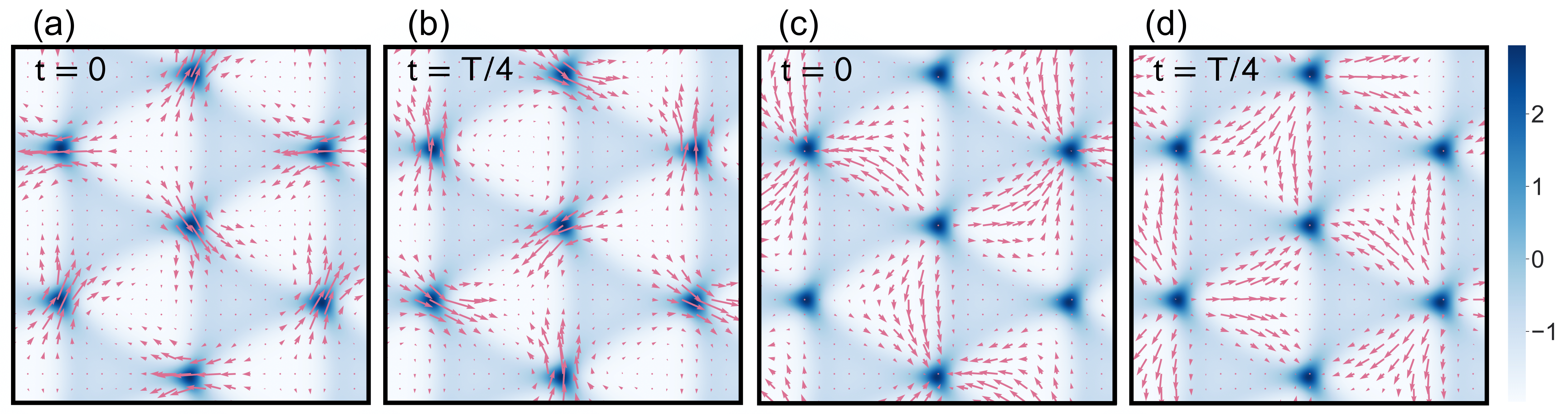
Figure S1: The twist angle is 1^∘ for the 180^∘ configuration MoS₂. The background is the interlayer binding potential of the relaxed structure. The dark blue regions are BA^′, the bigger white regions are AA^′ and the smaller light blue regions are AB^′. The real space displacement field $\delta\bm{u}^{-}(\bm{r},t)$ of the second lowest band at the $\bm{K}$ point at times (a) $t=0$ and (b) $t=T$/4 respectively, where $T$ is the time period. The real space displacement field for the third lowest band at times (c) $t=0$ and (d) $t=T/4$ respectively.

Angular Momentum

In this section we present the detailed steps on the calculation of phonon angular momentum shown in Fig. 3 and Fig. 5 in the main text. The phonon angular momentum is defined as [4, 5]:

$$L^{z}=\rho\int d^{2}\bm{r}\sum_{\ell=1,2}(\delta u_{x}^{(\ell)}\delta\dot{u}_{y}^{(\ell)}-\delta u_{y}^{(\ell)}\delta\dot{u}_{x}^{(\ell)})=\rho\int d^{2}\bm{r}\ \delta u^{T}(\bm{r})\ iM\ \delta\dot{u}(\bm{r})\;,$$ (S22)

where $M=I_{2}\otimes\sigma_{y}$ and $\delta u{(\bm{r})}=[\delta u_{x}^{(1)}(\bm{r}),\delta u_{y}^{(1)}(\bm{r}),\delta u_{x}^{(2)}(\bm{r}),\delta u_{y}^{(2)}(\bm{r})]^{T}$. For the unit cell number $n$ and the sublattice atom number $\alpha$, we have

$$\delta u_{n,\alpha}=\sum_{k}\tilde{\epsilon}_{k,\alpha}e^{i(\bm{k}\cdot\bm{R}_{n}-\omega_{k}t)}\sqrt{\frac{\hbar}{2\omega_{k}m_{\alpha}N}}a_{k}+h.c.\;,$$ (S23)

where $k=(\bm{k},\sigma)$, $\sigma$ is the band number, $m_{\alpha}$ is the mass of the $\alpha^{\text{th}}$ atom and $N$ is the number of unit cells. The eigenfunction $\tilde{\epsilon}_{k\alpha}=\sum_{G}\epsilon_{k\bm{G}}\ e^{i(\bm{k}-\bm{G})\cdot\bm{r}_{\alpha}}$, where $\epsilon_{k\bm{G}}$ are the coefficients of the block function solution to the central equation. The $\epsilon_{k,\bm{G}}$ can be obtained from Eq. S18 by setting $\bm{u}^{+}=0$ as we are calculating angular momentum for the $\bm{u}^{-}$ bands. The $\epsilon_{k\bm{G}}$ are normalized with respect to harmonics $\bm{G}$. The vector $\bm{r}_{\alpha}$ points to the $\alpha^{\text{th}}$ atom in moiré unit cell. In the case where all sublattices are the same, $m_{\alpha}=\rho\frac{A_{u}}{N_{u}}$, where $A_{u}$ is the area of the unit cell and $N_{u}$ are the number of atoms in the unit cell. Using $\bm{G}\cdot\bm{R}_{n}=2n\pi$, we obtain

$$\delta u(\bm{r})=\frac{1}{\sqrt{N_{u}}}\sum_{k\bm{G}}\epsilon_{k\bm{G}}e^{i((\bm{k}-\bm{G})\cdot\bm{r}-\omega_{k}t)}\sqrt{\frac{\hbar N_{u}}{2\omega_{k}\rho A_{u}N}}a_{k}+h.c.\;,$$ (S24)

where $\bm{r}$ is over the entire lattice. Writing the angular momentum

$$L^{z}=\frac{\hbar}{2A_{u}N}\int d^{2}\bm{r}\sum_{kk^{\prime}\bm{G}\bm{G}^{\prime}} \bigg{(}\epsilon_{k\bm{G}}^{\dagger}M\epsilon_{k^{\prime}\bm{G}^{\prime}}\sqrt{\frac{\omega_{k^{\prime}}}{\omega_{k}}}a_{k}^{\dagger}a_{k^{\prime}}$$

$$+\epsilon_{k^{\prime}\bm{G}^{\prime}}^{T}(-M)\epsilon^{*}_{k\bm{G}}\sqrt{\frac{\omega_{k}}{\omega_{k^{\prime}}}}a_{k^{\prime}}a^{\dagger}_{k}\bigg{)}e^{i[(\bm{k}^{\prime}-\bm{G}^{\prime})-(\bm{k}-\bm{G})]\cdot\bm{r}}e^{i(\omega_{k}-\omega_{k^{\prime}})t}\;,$$ (S25)

where we ignore the fast moving $aa$ and $a^{\dagger}a^{\dagger}$ terms. Since $\bm{k}$ runs only in the first brillouin zone and $\bm{G}$ are the reciprocal lattice vectors we have $\int d^{2}\bm{r}\ e^{i[\bm{k}^{\prime}-\bm{G}^{\prime}-(\bm{k}-\bm{G})]\cdot\bm{r}}=(2\pi)^{2}\delta(\bm{k}^{\prime}-\bm{k}-\bm{G}^{\prime}+\bm{G})\rightarrow{\delta_{\bm{k},\bm{k}^{\prime}}\delta_{\bm{G}\bm{G}^{\prime}}NA_{u}}$. Therefore

$$L^{z}=\frac{\hbar}{2}\sum_{k\bm{G}}\bigg{(}\epsilon_{k\bm{G}}^{\dagger}M\epsilon_{k\bm{G}}\ a_{k}^{\dagger}a_{k}+\epsilon_{k\bm{G}}^{T}(-M)\epsilon^{*}_{k\bm{G}}\ a_{k}a^{\dagger}_{k}\bigg{)}\;.$$ (S26)

We use the properties $\bm{\epsilon}_{k\bm{G}}^{T}(-M)\bm{\epsilon}_{k\bm{G}}^{*}=\bm{\epsilon}_{k\bm{G}}^{\dagger}M\bm{\epsilon}_{k\bm{G}}$ and $[a_{k},a^{\dagger}_{k}]=1$ to obtain

$${L^{z}}=\sum_{k}{L^{z}_{k}}\bigg{(}a_{k}^{\dagger}a_{k}+\frac{1}{2}\bigg{)}\;.$$ (S27)

In the main text we plot angular momentum at $k=(\bm{k},\sigma)$ given by $L^{z}_{k}=\sum_{\bm{G}}(\epsilon_{k\bm{G}}^{\dagger}M\epsilon_{k\bm{G}})\hbar$.

Berry Curvature

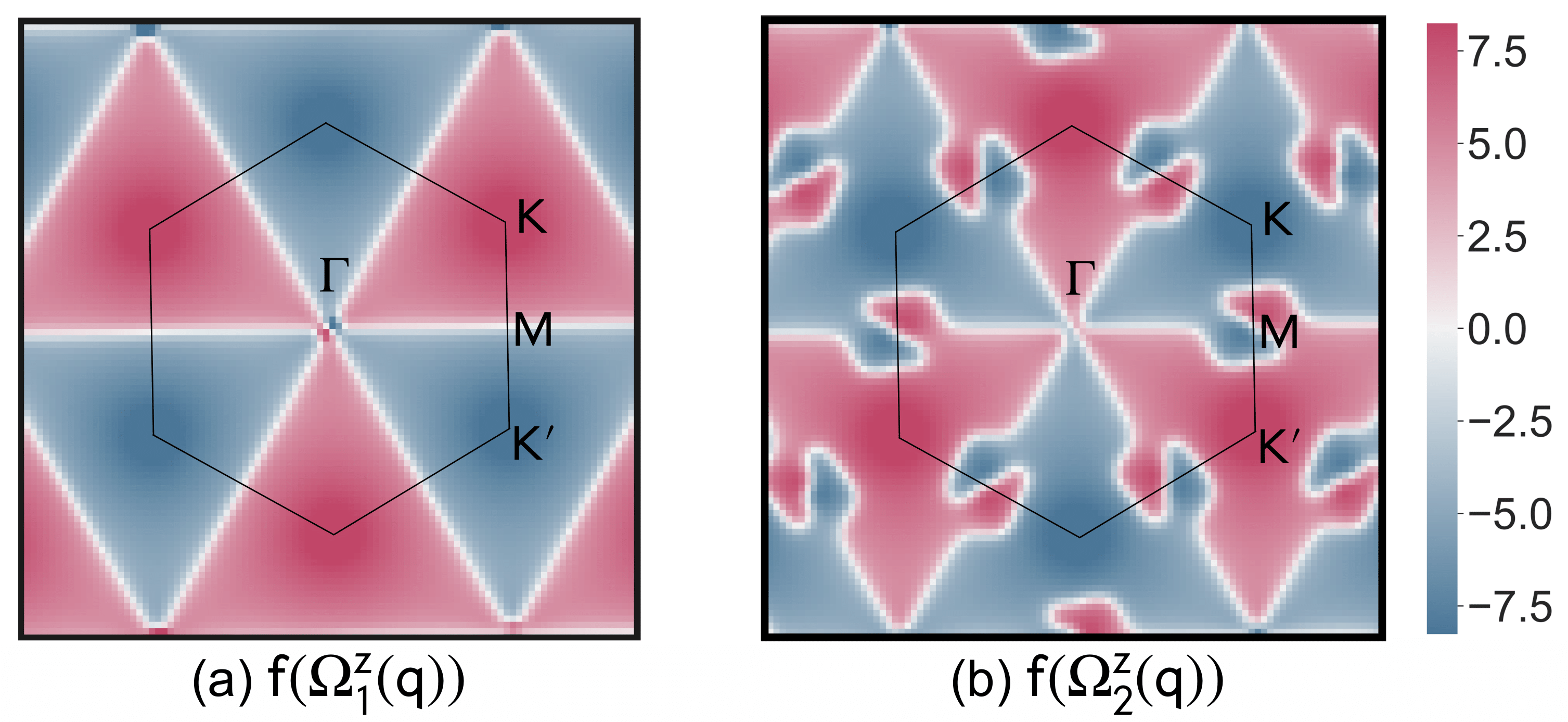
Figure S2: The log scaled Berry curvature of (a) the lowest and (b) the second lowest phonon band in the reciprocal space for the 180^∘ twisted bilayer MoS₂ at twist angle $\theta=2^{\circ}$. The scaling function is $f(\Omega^{z})=\text{sign}(\Omega^{z})\ln(1+|\Omega^{z}|)$

We follow the procedure in Ref.6 to calculate the phonon Berry curvature. We obtain the Hamiltonian from the Lagrangian using Legendre transformation and write it in Fourier space $H=\frac{1}{2}\sum_{q}\psi^{\dagger}_{\bm{q}}H_{\bm{q}}\psi_{\bm{q}}$. We define the basis as $\psi_{\bm{q}}=[\delta\tilde{u}^{-}_{({\bm{q}-\bm{G}})x},\delta\tilde{u}^{-}_{({\bm{q}-\bm{G}})y},\tilde{p}^{-}_{-({\bm{q}-\bm{G}})x},\tilde{p}^{-}_{-({\bm{q}-\bm{G}})y}]^{T}$ where each of the four operators $\delta\tilde{u}^{-}_{({\bm{q}-\bm{G}})\alpha}$, $\tilde{p}^{-}_{({\bm{q}-\bm{G}})\alpha}$ are $N$ dimensional, with $\bm{G}$ taking $N$ values given by $\bm{G}=m_{1}\bm{G}_{1}+m_{2}\bm{G}_{2}$ s.t. $m_{1},m_{2}\in\mathbb{Z}$. Here, we choose an appropriately large cutoff $N$, which is sufficient for convergence. The $4N\times 4N$ matrix $H_{\bm{q}}$ is given as

$$H_{\bm{q}}=\frac{1}{2}\begin{bmatrix}K_{\bm{q}}+V_{\bm{q}}&0\\ 0&\frac{\rho}{4}I_{2N}\end{bmatrix}\;,$$ (S28)

where $K_{q}$ is the spring constant matrix, given as

$$K_{\bm{q}}=\begin{bmatrix}\text{diag}\{(\lambda+2\mu)q^{2}_{x}+\mu q_{y}^{2}\}&\text{diag}\{(\lambda+\mu)q_{x}q_{y}\}\\ \text{diag}\{(\lambda+\mu)q_{x}q_{y}\}&\text{diag}\{(\lambda+2\mu)q^{2}_{y}+\mu q_{x}^{2}\}\end{bmatrix}\;,$$ (S29)

where each element is a $N$ dimensional diagonal matrix $\text{diag}\{{q}\}=\text{diag}(q-G_{0},\dots,q-G_{N-1})$. Similarly the interlayer interaction enters as

$$V_{\bm{q}}=-2V_{0}\sum_{j}\begin{bmatrix}a_{jx}^{*2}\ h^{j}&a_{jx}^{*}a_{jy}^{*}\ h^{j}\\ a_{jx}^{*}a_{jy}^{*}\ h^{j}&a_{jy}^{*2}\ h^{j}\end{bmatrix}\;,$$ (S30)

where the elements of matrix $h^{j}$ are given as $(h^{j})_{\bm{G},\bm{G}^{\prime}}=h^{j}_{\bm{G}-\bm{G}^{\prime}}$. The element $h^{j}_{\bm{G}}$ is calculated as $\cos(\bm{G}_{j}\cdot\bm{r}+\bm{a}_{j}^{*}\cdot\bm{u}_{0}^{-}+\phi)=\sum_{\bm{G}}h_{\bm{G}}^{j}e^{i\bm{G}\cdot\bm{r}}$. Using the Heisenberg equation of motion $i\partial_{t}\psi_{\bm{q}}=[\psi_{\bm{q}},H]$, we obtain $i\mathcal{J}\partial_{t}\psi_{\bm{q}}=H_{\bm{q}}\psi_{\bm{q}}$. The matrix $\mathcal{J}=[\psi_{\bm{q}},\psi_{\bm{q}}^{\dagger}]$ is given as

$$\mathcal{J}=2i\begin{bmatrix}0&I_{2N}\\ -I_{2N}&0\end{bmatrix}\;.$$ (S31)

We solve the eigenvalue problem $\omega_{n\bm{q}}\mathcal{J}\psi_{n\bm{q}}=H_{\bm{q}}\psi_{n{\bm{q}}}$. The Berry curvature defined as $\Omega_{n}^{z}=\partial_{q_{x}}A_{ny}-\partial_{q_{y}}A_{nx}$, where $\bm{A}_{n}=i\left\langle\psi_{n\bm{q}}\left|\mathcal{J}\partial_{\bm{q}}\right|\psi_{n\bm{q}}\right\rangle/\langle\psi_{n\bm{q}}|\mathcal{J}|{\psi}_{n\bm{q}}\rangle$.

We show the log-scaled berry curvature in Fig. S2 for the lowest two bands respectively in the reciprocal space. The log function is defined as $f(\Omega^{z})=\text{sign}(\Omega^{z})\ln(1+|\Omega^{z}|)$. The symmetry properties are similar to the angular momentum discussed in the main text. The higher band is slightly dissimilar to the lower band: it has another Berry curvature hot spot as a result of anti-crossing point with a higher band at the $\bm{M}$ point [see Fig. 2(b) in the main text].

Effective Model

The effective model of our chiral phonons is an extension of the effective model developed for twisted bilayer graphene by Koshino and Son [1]. As we discussed in the main text, there are two contributions to the total potential energy, those associated with domain walls and those associated with domains. The domain wall potential has been discussed by Koshino and Son. It is given by [1],

$$E_{\text{DW}}=\frac{1}{2}\sum_{\mathbf{q}}\tilde{\mathbf{u}}_{-\mathbf{q}}^{T}{D}^{DW}(\mathbf{q})\tilde{\mathbf{u}}_{\mathbf{q}}\;,$$ (S32)

where

$$D^{DW}_{\mu\nu}(\mathbf{q})=\sum_{i=1}^{3}\frac{\alpha V_{0}w_{d}}{2L_{M}}\left(2\sin\frac{\mathbf{q}\cdot\mathbf{L}_{i}^{M}}{2}\right)^{2}\left[\delta_{\mu\nu}-\frac{\left(\mathbf{L}_{i}^{M}\right)_{\mu}\left(\mathbf{L}_{i}^{M}\right)_{v}}{L_{M}^{2}}\right]\;.$$ (S33)

where $w_{d}\approx\frac{a}{4}\sqrt{\frac{2(\lambda+\mu)}{V_{0}}}$ is the width of domain walls, $\bm{L}_{i}$ are the first star of moiré lattice vectors such that $L_{M}=|\bm{L}_{i}|$   . It satisfies the property ${D}^{\text{DW}}(\bm{q})={D}^{\text{DW}}(-\bm{q})$, i.e., $E_{\text{DW}}$ does not break $C_{2z}$.

In the main text, we argued that when the interlayer binding energy breaks $C_{2z}$ symmetry, there is an additional potential energy associated with the area change of the stacking domains,

$$E_{\text{Domain}}=\frac{1}{2}\sum_{\mathbf{q}}\tilde{\mathbf{u}}_{-\mathbf{q}}^{T}D^{\text{Domain}}(\mathbf{q})\tilde{\mathbf{u}}_{\mathbf{q}}=\alpha\frac{(V_{AA^{\prime}}-V_{AB^{\prime}})}{2}\sum_{\mathbf{q}}\tilde{\mathbf{u}}_{-\mathbf{q}}^{T}\begin{bmatrix}0&\gamma_{AA^{\prime}}(\bm{q})\\ -\gamma_{AA^{\prime}}(\bm{q})&0\end{bmatrix}\tilde{\mathbf{u}}_{\mathbf{q}}\;,$$ (S34)

where

$$\gamma_{AA^{\prime}}(\bm{q})=4i\sin(\frac{\bm{q}\cdot(\bm{L_{2}-L_{1}})}{2})\sin(\frac{\bm{q}\cdot\bm{L_{1}}}{2})\sin(\frac{\bm{q}\cdot\bm{L_{2}}}{2})$$ (S35)

with $\bm{L}_{1}$ and $\bm{L}_{2}$ being the moiré lattice vectors. It must be noted that only bilinear terms in displacement contribute to the change in area as the linear terms average out to zero. For twisted bilayer graphene, the AA regions have the highest energy, therefore $E_{\text{Domain}}\propto V_{AB}-V_{BA}$. Since $V_{AB}=V_{BA}$, this term does not appear in Koshino and Son’s model.

Combining $E_{\text{DW}}$ and $E_{\text{Domain}}$ together, the equation of motion is given by

$$M\ddot{\bm{\tilde{u}}}_{\bm{q}}=-[D^{\text{DW}}+D^{\text{Domain}}]\bm{\tilde{u}}_{\bm{q}}\;,$$ (S36)

where $M=\rho(a/w_{d})^{2}w_{d}L_{M}$ is the effective mass [1]. Solving the above equation yields the phonon band dispersion of the effective model shown in Fig. 4(d) in the main text.

References

- Koshino and Son [2019] M. Koshino and Y.-W. Son, Moiré phonons in twisted bilayer graphene, Phys. Rev. B 100, 075416 (2019).
- Ochoa [2019] H. Ochoa, Moiré-pattern fluctuations and electron-phason coupling in twisted bilayer graphene, Phys. Rev. B 100, 155426 (2019).
- Carr et al. [2018] S. Carr, D. Massatt, S. B. Torrisi, P. Cazeaux, M. Luskin, and E. Kaxiras, Relaxation and domain formation in incommensurate two-dimensional heterostructures, Phys. Rev. B 98, 224102 (2018).
- Zhang and Niu [2015] L. Zhang and Q. Niu, Chiral phonons at high-symmetry points in monolayer hexagonal lattices, Phys. Rev. Lett. 115, 115502 (2015).
- Zhang and Niu [2014] L. Zhang and Q. Niu, Angular momentum of phonons and the einstein–de haas effect, Phys. Rev. Lett. 112, 085503 (2014).
- Zhang et al. [2019] X. Zhang, Y. Zhang, S. Okamoto, and D. Xiao, Thermal Hall effect induced by magnon-phonon interactions, Phys. Rev. Lett. 123, 167202 (2019).
- Note [1] Koshino and Son in Ref. 1 take as the binding potential energy constant compared to used in this letter. The expression for has a factor of half to account for the change.