Pseudo-mask Matters in Weakly-supervised Semantic Segmentation

Abstract

Most weakly supervised semantic segmentation (WSSS) methods follow the pipeline that generates pseudo-masks initially and trains the segmentation model with the pseudo-masks in fully supervised manner after. However, we find some matters related to the pseudo-masks, including high quality pseudo-masks generation from class activation maps (CAMs), and training with noisy pseudo-mask supervision. For these matters, we propose the following designs to push the performance to new state-of-art: (i) Coefficient of Variation Smoothing to smooth the CAMs adaptively; (ii) Proportional Pseudo-mask Generation to project the expanded CAMs to pseudo-mask based on a new metric indicating the importance of each class on each location, instead of the scores trained from binary classifiers. (iii) Pretended Under-Fitting strategy to suppress the influence of noise in pseudo-mask; (iv) Cyclic Pseudo-mask to boost the pseudo-masks during training of fully supervised semantic segmentation (FSSS). Experiments based on our methods achieve new state-of-art results on two changeling weakly supervised semantic segmentation datasets, pushing the mIoU to 70.0% and 40.2% on PAS-CAL VOC 2012 and MS COCO 2014 respectively. Codes including segmentation framework are released at https://github.com/Eli-YiLi/PMM

1 Introduction

Semantic segmentation is a fundamental computer vision problem and requires time-consuming pixel-level manual annotations. To reduce the annotation burden, weakly-supervised semantic segmentation approaches have been proposed using scribble annotations [23, 32], bounding boxes [36, 9, 16] , points [3] or image-level labels [17, 27, 28, 2, 33]. In this paper, we focus on weakly-supervised semantic segmentation with image-level labels due to its easily available annotations.

Almost all the latest WSSS algorithms require pseudo-mask derived from CAM to train the FSSS model. Instead of the pseudo-mask, previous works mainly focus on the generation of CAMs, or the post-process of them. We observe that there are some matters about pseudo-mask that are not handled appropriately as follows: (i) argmax operation on the CAMs along the channel dimension projects multi-label class activation maps (CAMs) to single-label pseudo-masks, but the image-level classification for generating CAMs does not consider the conflicts of predictions on target locations; (ii) CAMs generated by the classification model tend to focus on the most discriminative part and result in partial activations; (iii) the noise in pseudo-masks is inevitable and impedes the training of fully-supervised semantic segmentation (FSSS). (iv) the predictions of FSSS are usually more accurate than supervisory signals (pseudo-masks).

In this paper, we propose a series of strategies to boost the efficiency of pseudo-masks in aspects of both generation and utilization. Specifically, in the pseudo-mask generation step, we firstly compute the Coefficient of Variation ($c_{v}$) for each channel of CAMs, and then refine CAMs via exponential functions with $c_{v}$ as the control coefficient. This operation smooths the CAMs and could alleviate the partial response problem introduced by the classification pipeline. Instead of projecting the three-dimensional CAM after dense-CRF [18] directly to two-dimensional pseudo-mask with the argmax operation on scores as in previous studies, we equip each pixel a scalar which is computed as the proportion between the pixel’s attention and the attention sum of the channels over the whole image. Intuitively the scalar represents the importance of the corresponding pixel based on which the final pseudo-masks are generated. In the FSSS training step, we propose a Pretended Under-fitting Strategy which suppresses the losses of the noise labels in the pseudo-masks. In addition, the model is evaluated on validation dataset and we update the masks cyclically in condition that prediction from model is better than the pseudo-masks, rather than use the fixed pseudo-masks generated in the first step.

Applying our methods to a baseline algorithm called SEAM [33], we achieve new state-of-the-art results on two challenging weakly-supervised semantic segmentation benchmarks. In particular, our approach reach the mIoU of 70.0% and 40.2% on In PASCAL VOC 2012 [10] and MS COCO 2014 [24] validation sets respectively.

The contributions of this paper are three-fold:

• We generate high-quality pseudo-masks by the proposed Proportional Pseudo-mask Generation with Coefficient of Variation Smoothing. The Coefficient of Variation Smoothing expands the activation area of CAMs to overcome the partial response problem based on the CAM’s coefficient of variation, and the Proportional Pseudo-mask Generation computes the importance of each location for each class independently, based on which the final pseudo-masks are generated.

• We realize the effective utilization of pseudo-masks via reducing the influence of noise by our Pretended Under-fitting Strategy, and narrow the gap between ground-truths and pseudo-masks via Cyclic Pseudo-masks. The pixel-wise losses are reweighted to suppress the noises in the Pretended Under-fitting Strategy and pseudo-masks are refined in a iterative manner.

• We conduct extensive experiments to validate the effectiveness of our proposed approach (Pseudo-mask Matters, PMM), and demonstrate that our approach achieves new state-of-the-art results on two challenging weakly-supervised semantic segmentation datasets.

2 Related Work

Weakly Supervised Semantic Segmentation: What WSSS does is to simplify the supervision with less accuracy loss. The annotation cost weakens from mask [7, 40] (fully supervision) to scribble [23, 32], bounding box [36, 9, 16], points [3] and image label [17, 27, 28, 2, 33] gradually. Till image-level label, there is only category information without spatial supervision. Thanks to the translation invariance of CNNs, the classification contributed pixels keep high response in the feature map. After combining the weights of classifier with the feature map, we get the CAM [42] as the initial semantic mask. Later works mostly focus on expanding the seed areas. The methods include adding CRF and dilation [34], designing new losses [17], erasing high response area [13], keeping scale consistency via siamese network and correlation module [33], clustering sub-categories for classification [5]. Besides CAM based methods, weakly supervised object detection method is also used with proposal models [25].

For the overall pipeline of WSSS, firstly a binary classification model is trained to obtain the CAMs and several techniques have been proposed to improve its quality. Secondly post-processing has been applied on the CAMs to generate pseudo-masks. Finally, semantic segmentation model with pseudo-masks supervised is trained in fully supervised manner.

Pseudo-mask Generation: Pseudo-mask generation is to project three-dimensional CAM to two-dimensional pseudo-mask with some post-process algorithms. Following the manner of single label classification, the pixel-level labels are identified by argmax operation on the CAMs along the channel dimension after post-process, although the model to predict the CAMs is trained by binary classifiers which exclude the label competition.

Conditional Random Fields (CRF), a sort of statistical modeling method for structured prediction with considering neighboring samples, has been widely used as the post processing tool for segmentation. Some variations of CRF have been proposed. Dense-CRF [18] applies the appearance kernel to link nearby pixels with similar color, and smoothness kernel to removes small isolated regions. Deeplabv1 [6] is an early work that introduces fully connected CRF in to segmentation task as post process. Then, CRFasRNN [41] combines the CNN and CRF end-to-end. Besides, DPN [26] uses the MRF which is similar to CRF. Further more, G-CRF [4] introduced CNN for potential learning to improve the performance.

Several post-process methods based on deep learning have also been proposed. [2, 1] learn the contour of objects via an affinity network in inference stage. The training masks are synthesised from two CRF results with different background intensities. Besides the unsupervised contour learning method, other works introduce saliency detection models trained from extra dataset to refine CAMs [37, 38, 11].

3 Methodology

In this section, We firstly elaborate the traditional pipeline generating pseudo-mask which projects the class activation map $\boldsymbol{X}\in\mathbb{R}^{C\times H\times W}$ to pseudo-mask $\boldsymbol{Y}\in\mathbb{R}^{H\times W}$ with CRF function $crf$ and image $\boldsymbol{I}$. Then we introduce our pseudo-mask generation method, Proportional Pseudo-mask Generation (PPMG) with Coefficient of Variation Smoothing (CVS) as Fig. 1. After that, the noise suppressing module, Pretended Under-fitting Strategy (PUS) for the FSSS is described. Finally, the overall pipeline with Cyclic Pseudo-masks (CPM) involved is presented. We name our pipeline PMM from the abbreviation of Pseudo-mask Matters.

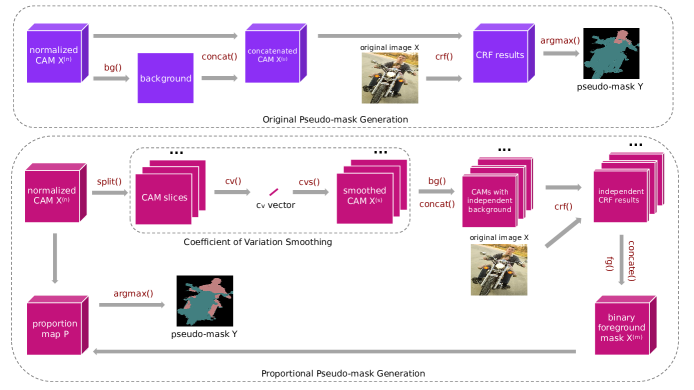
Figure 1: Illustration of pseudo-mask generation. Top: traditional pipeline for pseudo-mask generation. Bottom: Proportional Pseudo-mask Generation with Coefficient of Variation Smoothing. $cv$ counts the coefficient of variation for each channel and $cvs$ smooths the CAM. $bg$ generates the background with exponential function and $fg$ returns the binary foreground. $p$ counts the proportion of a pixel to the entire category.

3.1 Pseudo-mask Generation with CRF

The CRF algorithm $crf$ here is dense-CRF [18]. The CAMs are processed with operations, including normalization $norm$, exponentially background generation $bg$ and $argmax$, and the results are set as the input to CRF.

Specifically, Min-Max Normalization is applied on $\boldsymbol{X}_{c,:,:}$ and formulated as:

$$norm(\boldsymbol{X}_{c,h,w})=\frac{\boldsymbol{X}_{c,h,w}-min(\boldsymbol{X}_{c,:,:})}{max(\boldsymbol{X}_{c,:,:})-min(\boldsymbol{X}_{c,:,:})},\forall c,h,w$$ (1)

where $h$ and $w$ are the coordinates on the CAMs, and $c$ represents the channel index.

After normalization for each pixel, we have $\boldsymbol{X}^{(n)}$. Then the normalized pixel $\boldsymbol{X}_{c,h,w}^{(n)}$ on background matrix is constructed exponentially with power $\alpha$ from the normalized foreground pixels $\boldsymbol{X}_{:,h,w}^{(n)}$ in location $h$ and $w$:

$$bg(\boldsymbol{X}_{:,h,w}^{(n)})=(1-max(\boldsymbol{X}_{:,h,w}^{(n)}))^{\alpha},\forall h,w$$ (2)

Then concatenate the background and foreground to form the input $\boldsymbol{X}^{(u)}$ of unary potential function in CRF:

$$\boldsymbol{X}^{(u)}=concat(bg(\boldsymbol{X}^{(n)}),\boldsymbol{X}^{(n)})$$ (3)

Finally, the pseudo-mask is identified via argmax operation in category channel after CRF:

$$\boldsymbol{Y}=argmax(crf(\boldsymbol{I},\boldsymbol{X}^{(u)})),$$ (4)

3.2 Coefficient of Variation Smoothing

The motivation of Coefficient of Variation Smoothing (CVS) is to smooth the class activation map based on the variation of confidence in spatial domain. We believe different images and classes require varied smoothing intensity depending on its distribution of confidences. To measure it, we introduce the Coefficient of Variation ($c_{v}$) as the metric for the foreground pixels $\boldsymbol{X}_{c,:,:}^{(f)}$ whose scores are higher than threshold $t$ in normalized metric $\boldsymbol{X}_{c,:,:}^{(n)}$ at channel $c$. We define the $cv$ function in Eq.(5) where $\mathbb{D}$ counts the deviation $\sigma^{2}$ and $\mathbb{E}$ counts the mean $\mu$.

$$cv(\boldsymbol{X}_{c,:,:}^{(n)})=\frac{\sqrt{\mathbb{D}(\boldsymbol{X}_{c,:,:}^{(f)})}}{\mathbb{E}(\boldsymbol{X}_{c,:,:}^{(f)})},$$ (5)

Then the $c_{v}$ is used as exponential function power to each pixel. As $\boldsymbol{X}^{(n)}\in[0,1]$, lower exponential power under 1 leads smaller differences between the foreground pixels and smooths the CAM. Here, We define the $cvs$ for each pixel with scale factor $s$ as:

$$cvs(\boldsymbol{X}_{c,h,w}^{(n)},(c_{v})_{c})=(X_{c,h,w}^{(n)})^{(1-s\times(c_{v})_{c})},\forall c,h,w$$ (6)

The CVS is applied after the normalization operation Eq.(1), and expand the activation area of target objects. Experimentally, CVS works more efficiently with stronger augmentations involved, which also requires more training iterations.

3.3 Proportional Pseudo-mask Generation

One important concern in WSSS is that the CAMs are obtained from binary classifiers. Follow the independent manner of binary cross entropy loss, we generate class-specific background for the smoothed CAM $\boldsymbol{X}_{c,:,:}^{(s)}$ by $bg$ and apply $crf$ for it, then we return the binary foreground via $fg$, thus we have $\boldsymbol{X}_{c,:,:}^{(m)}$ as:

$$\boldsymbol{X}_{c,:,:}^{(m)}=fg(crf(\boldsymbol{I},bg(\boldsymbol{X}_{c,:,:}^{(s)}))),\forall c$$ (7)

In this function, $fg$ sets the foreground pixels whose scores are upper than $t$ to 1, and other pixels to 0. So $\boldsymbol{X}_{c,:,:}^{(m)}$ is a binary class mask. Then we concatenate the masks to $\boldsymbol{X}^{(m)}$.

However, more than one labels may be assigned to some pixels as activation areas of different classes could be overlapped. We do not assign the label to each pixel by activation scores on CAM, because in binary cross entropy, the loss only requires the network to distinguish positive sample and negatives for each category independently, and thus highlights the foreground consequently. But scores of different categories on foreground areas are not competitive during the training of binary classification. So rather than taking the index of the highest score as pseudo label, we compute a metric indicating the importance of each class on each pixel, based on which the pixel is assigned with more important label. Specifically, the CRF map is converted to a binary mask with the a thresholding operation and the computation of metric mention before could not be affected by the CRF score. The proportion function $p$ is defined as:

$$p(\boldsymbol{X}_{c,h,w}^{(n)})=\frac{\boldsymbol{X}_{c,h,w}^{(n)}}{sum(\boldsymbol{X}_{(c,:,:)}^{(n)}\cdot\boldsymbol{X}_{c,:,:}^{(m)})},\forall c,h,w$$ (8)

In Eq.(8) $\boldsymbol{X}_{c,:,:}^{(m)}$ is the foreground binary mask in channel $c$. Then, argmax is operated on the element-wise multiplication of mask and proportion map along channel dimension to generate pseudo-mask and formulated as:

$$\boldsymbol{Y}=argmax(\boldsymbol{X}^{(m)}\cdot\boldsymbol{P})$$ (9)

Thus, each pixel is equipped with a single label after the processing above and could be serve as supervision for semantic segmentation training.

The pseudo implementation of Proportional Pseudo-mask Generation is described in Alg.(1) :

Algorithm 1 Proportional Pseudo-mask Generation

Input: image $\boldsymbol{I}$ and CAM $\boldsymbol{X}\in\mathbb{R}^{C\times H\times W}$

Output: pseudo-mask $\boldsymbol{Y}\in\mathbb{R}^{H\times W}$

  1: normalize the CAM: $\boldsymbol{X}^{(n)}=norm(\boldsymbol{X})$

  2: count $c_{v}$ for each class: $c_{v}=cv(\boldsymbol{X}^{(n)})$

  3: smooth the CAM: $\boldsymbol{X}^{(s)}=cvs(\boldsymbol{\boldsymbol{X}}^{(n)},c_{v})$

  4: compute binary mask with $crf$:

       $\boldsymbol{X}_{c,:,:}^{(m)}=fg(crf(\boldsymbol{I},bg(\boldsymbol{X}_{c,:,:}^{(s)}))),\forall c$

  5: count the proportion map: $\boldsymbol{P}=p(\boldsymbol{X}^{(n)})$

  6: generare pseudo-mask: $\boldsymbol{Y}=argmax(\boldsymbol{X}^{(m)}\cdot\boldsymbol{P})$

3.4 Pretended Under-fitting Strategy

Compared with the manual annotations, pseudo-masks that serves as supervision signal to train the semantic segmentation are noisy. Previous studies focus on the generation of high quality pseudo-masks to reduce the noise and rare of them attempt to suppress the noise during the model training. Our approach is to reweight the losses of potential noise pixels in the optimization of FSSS. For this goal, we propose the Pretended Under-fitting Strategy as Eq.(10):

$$\ell(\boldsymbol{L})=\begin{cases}mean(\boldsymbol{L})&mean(\boldsymbol{L})>=\beta\\ mean(pus(\boldsymbol{L}))&mean(\boldsymbol{L})<\beta\end{cases}$$ (10)

$\boldsymbol{L\in}\mathbb{R}^{H\times C}$ is the loss map for pixels in the image from cross entropy loss, and $\ell$ means the loss of Pretended Under-fitting Strategy for the loss map $\boldsymbol{L}$. Funtion $pus()$ is the operation of Pretended Under-fitting Strategy if the mean value of $\boldsymbol{L}$ below warm up threshold $\beta$.

Three operations are implemented as followed:

$$pus_{clamp}(\boldsymbol{L})=\begin{cases}\boldsymbol{L}_{h,w}&\boldsymbol{L}_{h,w}<\kappa\\ \boldsymbol{L}_{h,w}\cdot\frac{\kappa}{\boldsymbol{L}_{h,w}}&\boldsymbol{L}_{h,w}>=\kappa\end{cases}\forall h,w$$ (11)

$$pus_{pow}(\boldsymbol{L})=\boldsymbol{L}^{\kappa}$$ (12)

$$pus_{ignore}(\boldsymbol{L})=\begin{cases}\boldsymbol{L}_{h,w}&\boldsymbol{L}_{h,w}<\kappa\\ 0&\boldsymbol{L}_{h,w}>=\kappa\end{cases}\forall h,w$$ (13)

$pus_{clamp}$ sets a maximum of $\boldsymbol{L}$ to a hyper parameter $\kappa$ while $pus_{ignore}$ drops these pixels. $pus_{pow}$ carries out a scaling strategy by exponential function. We later evaluate these operations in Tab. 4.

3.5 Cyclic Pseudo-mask and Overall Pipeline

Obviously there is a large gap between pseudo-mask and real ground-truth. Previous studies have shown that CNN model is robust to noise in some degree. So a simple but effective method to narrow the gap is to update the pseudo-mask cyclically. We replace the pseudo-mask on training dataset as the predictions from the trained model on it. We call the new mask as Cyclic Pseudo-mask. This operation is validated in next section.

The overall pipeline is consisted of (i) classification for CAMs, (ii) pseudo-mask generation and (iii) training of FSSS. In the first step, multi-crop test is used to generate the CAMs instead of multi-scale test. Specifically, Multi-crop firstly resizes the image to different resolutions and crop the resized images with fixed crop size and stride, then compute the average of crop results. Meanwhile, we propose a multi-crop training technique which transforms the image in the similar way to the test. Note that, we need a base mask to update the ground truth, as multi-crop may crops the background if the image is resized too large, causing the original labels invalid. In our study, the CAMs from SEAM [33] are used as the base mask. The scale-friendly CNN structure, ScaleNet [22], is applied to train the classification model and multi-crop operation which loads the rough mask and update the image level label is implemented online.

4 Experiments

4.1 Implementation Setup

Datasets: We evaluate our approach on PASCAL VOC 2012 dataset and MS-COCO 2014 dataset. All the mask annotations are converted to image level multi-label ground-truths. VOC12 contains 20 foreground objects and one background. The dataset is divided into train set (1464 images), validation set (1449 images) and test set (1456 images). In general, additional annotations from SBD [12] are used to augment training set to 10582 images. COCO14 dataset ranges from 1 to 90, among them 80 categories are valid foreground. The train set contains 82081 images and the number of validation set is 40137. We evaluate the experiments on the validation sets by Mean intersection over union (mIoU).

Implementation details: Our baseline of classification framework is SEAM. We replace the backbone from Wide ResNet38 [35] in SEAM to ScaleNet101 [22] to boost the multi-scale feature which is similar to multiple resolution training in SEAM. The output stride is 8 without extra dilations since the receptive fields of ScaleNet is massive. Feature maps from stage 3 and stage 4 are projected to 64 and 128 channels respectively by 1$\times$1 convolution layers for the PCM module in SEAM.

The resize scales of multi-crop start from 0.75 to 3 (step 0.25). The resized images are cropped in size 448$\times$448 with crop stride 300. In train phase, if crop area covers over 10% of foreground class $c$ or over 10% area of crop is class $c$, we tag the ground-truth to positive in channel $c$. The training images is randomly selected from the multi-crop proposals. In test phase, the resize scales, crop size and stride are the same to train phase. We get the base mask from original SEAM with $\alpha$ in CRF setting to be 24 without Random Walk. SEAM is trained as original settings. Note that multi-crop training requires 20 epochs to make sure that each cropped patch of images are involved. The initial learning rate:wq is set to 0.02 with batch size 16. The CAM background exponent $\alpha$ and the scale factor $s$ of $cvh$ function are obtained from grid search (eg. 11 and 0.3), with foreground threshold $t$ at 0.05.

For the fully supervised segmentation, we do not reproduce the performance of deeplab-v2 [7] as described in [33], so we use the PSPnet [40] to achieve the mIoU in the paper with codebase MMSegmentation [8]. We follow the settings in MMSegmentation for VOC, and we add dense-CRF to it. For Pretended Under-fitting Strategy, set the warm up threshold $\beta$ and hyper parameter $\kappa$ in PUS to 0.5 for VOC, and 0.8 for COCO. The training batch size is 16 on 8 gpus at learning rate 0.005 for 20000 iterations in ploy policy. On VOC12 dataset, the pseudo-mask is updated once according to the method described in 3.5 and we do only apply the pretended under-fitting strategy in the 1st round training. On COCO14 dataset, the pseudo mask is not updated as we observe that the performance on validation dataset is the best after the 1st round training. We set the class number to 91 (one background and 10 invalid), and the invalid classes are ignored in test. Besides that, we use 32 gpus, batch size 64, learning rate 0.02 and iteration 40000 for the training of COCO14. All of the backbones in FSSS are initialized with the pretrained model from ImageNet[19].

4.2 Ablation Studies

We make ablation studies for CAM generation, pseudo-mask generation and segmentation in different settings. All the results are evaluated on validation set of VOC12 for the consistency of comparison.

Improvements of CAM: In this paper, we push out a strong CAM baseline based on multi-crop and multi-scale network. In Tab. 1, the top part evaluates the effectiveness of multi-crop strategy. Notable, there is 3.49 improvement when multi-crop is applied on both train and test phase, compared to 1.21 in test phase only. Then we compare multi-scale backbones in the middle part, and we find the ScaleNet101 performs significantly better than Res2Net101 and wide ResNet38, which suggests that apply multi-scale operations in backbone benefits CAMs a lot. We add multi-crop to train phase in last line for ScaleNet101, and the final result is 58.21.

Setting	Backbone	VOC12 val
baseline	ResNet38	52.72
multi-crop test	ResNet38	53.93
multi-crop test & train	ResNet38	56.21
multi-crop test	Res2Net101	54.90
multi-crop test	ScaleNet101	57.81
multi-crop test & train	ScaleNet101	58.21

Table 1: CAM mIoU of different settings.

Improvements of Pseudo-mask Generation: We evaluate the effectiveness of CVS and PPMG in Tab. 2. We firstly apply dense-CRF on baseline (SEAM) and our variant in the top part. The mIoU of CAMs increases by 1.52 and 0.98 respectively in these two settings. These results are obtained from grid search of CRF background reduction hyper parameter $\alpha$ from 0 to 20. In the middle part, we show the individual gains and we find the gains of PPMG are more. In the last line, PPMG with CVS and CRF improves the baseline by 4.6, and the gain of our CAM is 3.28. In Fig. 2 we give some examples with its $c_{v}$ values and its results after CVS, we can observe that the disparity problem is more critical with larger $c_{v}$ values and CVS could handle it appropriately.

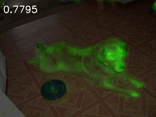
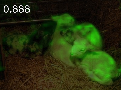
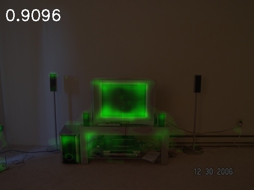
Figure 2: Visualization of CAM and its Coefficient of Variation. Top: CAM. Bottom: CAM after CVS. Only one category is highlighted in these images.

Setting	Baseline	Ours
CAM	52.72	58.21
CRF	54.24	59.19
CRF & CVS	54.41	60.83
PPMG without CVS	57.02	61.23
PPMG	57.32	61.49

Table 2: CAM mIoU of different post-process settings on VOC12 val set. CVS: Coefficient of Variation Smoothing. PPMG: Proportional Pseudo-mask Generation. Baseline CAM results are from SEAM, and “Ours” adds multi-crop and ScaleNet.

Removal of Random Walk: Most WSSS algorithms deploy Random Walk to refine the CAM. It requires CRF operations at different $\alpha$ values to synthesize the training data. However, the results in Tab. 3 suggest that the affinity network and Random Walk do not work in our settings. So we remove the affinity network and Random Walk in our pipeline. The visualization of our refined CAM is depicted in Fig. 3 with baseline SEAM.

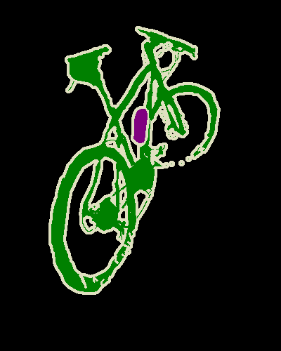
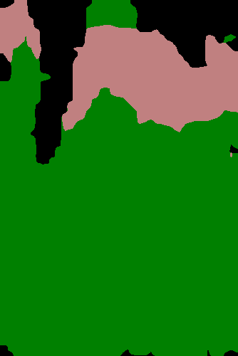
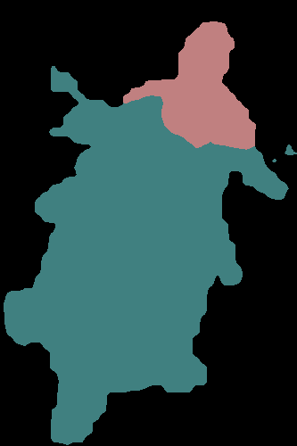
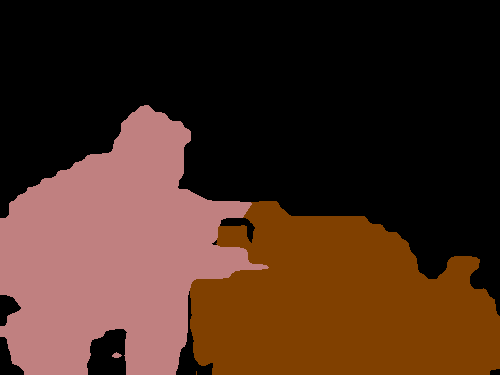
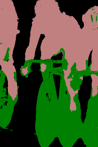
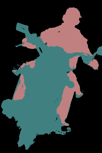
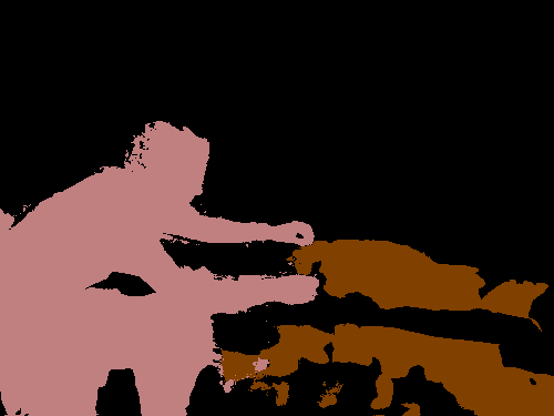
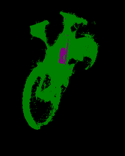
Figure 3: Qualitative results of pseudo-maskt. Top: original images in VOC12 validation set. Second row: ground truth with ignored boundary. Third row: pseudo-masks of SEAM (baseline) with Random Walk. Bottom : our pseudo-masks from PPMG with CVS.

our CAM	CRF	RW	PPMG	VOC12 val
$\checked$				58.21
$\checked$	$\checked$			59.19
$\checked$		$\checked$		52.18
$\checked$			$\checked$	61.49
$\checked$		$\checked$	$\checked$	60.96

Table 3: mIoU of different post-process settings.

Improvements of Pseudo-mask Utilization: We firstly compare three $pus$ operations in Tab. 4. The top part shows the results from different pseudo-masks without PUS. The middle part shows the results of three $pus$ functions, among which, $pus_{clamp}$ performs best. Compared to baseline pseudo-mask, the improvement rises from 0.45 to 3.46 after applying the $pus_{clamp}$, which means the PUS is essential to our pipeline.

$pus$	Pseudo-Mask	VOC12 val
-	SEAM & RW	64.41
-	Ours	64.86
pow	Ours	64.92
ignore	Ours	65.44
clamp	Ours	66.73
clamp	SEAM & RW	63.27

Table 4: Comparison of Pretended Under-fitting Strategy.

We also validate the effectiveness of Cyclic Pseudo-mask in Tab. 5. We find VOC dataset needs to update the pseudo-mask once while COCO does not require cyclically updating.

Cycle Times	V0C val	COCO val
0	66.73	36.73
1	68.50	35.65
2	68.27	-

Table 5: Performance of Cyclic Pseudo-mask in different cycle times. 0 suggests non-cyclic pseudo-mask.

In Tab. 6, We show the accumulated gains of our methods, including the classification, segmentation and pseudo-mask generation methods. Although our classification pipeline improve the performance of CAM, application of RW instead of PPMG hurts the performance.

Ori	Cls	RW	PPMG	PUS	Cyclic	R2N	mIoU
$\checked$							52.72
$\checked$	$\checked$						58.21
$\checked$	$\checked$	$\checked$					52.18
$\checked$	$\checked$		$\checked$				61.49
$\checked$	$\checked$		$\checked$	$\checked$			66.73
$\checked$	$\checked$		$\checked$	$\checked$	$\checked$		68.50
$\checked$	$\checked$		$\checked$	$\checked$	$\checked$	$\checked$	70.01

Table 6: Accumulated gains on V0C12 validation set. Cls means our classification setting. RW is affinity with Random Walk. PPMG is Proportional Pesudo-mask Generation with CVS. PUS is fully-supervised segmentation with Pretended Under-fitting Strategy. Cyclic indicates Cyclic Pseudo-mask. R2N change the backbone of segmentation to Res2Net.

4.3 Comparison with State-of-the-arts

We compare the final results after fully supervised segmentation step in Tab. 7. The backbones of segmentation framework are listed in the table. Our method does not require affinity network and Random Walk inference, while achieves new state-of-the-arts in both VOC12 and COCO14 validation datasets at 70.0 and 40.2 respectively. Compared to our baseline SEAM, the gain is 5.5 in VOC12 and 5.0 in COCO14. For the same backbone, the improvements are 4.0 and 5.0 respectively. Note that the performance of ScaleNet101 on VOC is lower than base model ResNet38, but it suits tiny objects well on COCO at mIoU 40.2.

Method	Backbone	RW	val	test	COCO
BFBP [29]	VGG16	$\mathsf{x}$	46.6	48.0	20.4
SEC [17]	VGG16	$\mathsf{x}$	50.7	51.7	22.4
AffinityNet [2]	ResNet38	$\checked$	61.7	63.7	-
IRNet [1]	ResNet50	$\checked$	63.5	64.8	-
OAA [15]	ResNet101	$\mathsf{x}$	63.9	65.6	-
ICD [11]	ResNet101	$\mathsf{x}$	64.1	64.3	-
SEAM [33]⋆	ResNet38	$\checked$	64.4	65.7	-
SEAM [33]	ResNet38	$\checked$	64.5	65.7	31.7
SSDD [30]	ResNet	$\checked$	64.9	65.5	-
CONTA [39]	ResNet38	$\checked$	66.1	66.7	32.8
SC-CAM [5]	ResNet101	$\checked$	66.1	65.9	-
Sun et al. [31]	ResNet101	$\checked$	66.2	66.9	-
PMM	ResNet38	$\mathsf{x}$	68.5	69.0	36.7
PMM	ScaleNet101	$\mathsf{x}$	67.1	67.7	40.2
PMM	Res2Net101	$\mathsf{x}$	70.0	70.5	35.7

Table 7: Performance comparisons with state-of-the-art WSSS methods on VOC 2012 and COCO 2014 validation datasets. All the methods listed use image-level supervision only without extra models. Checkmarks suggest these methods need training an affinity network and Random Walk inference. SEAM in blue is our baseline and^⋆ indicates our re-implementation baseline in same segmentation code.

In Tab. 8 we compare our PMM to methods with extra information like saliency model, bounding box supervision, extra dataset and segment-based object proposals. These methods introduce more information and thus take advantage to the methods in Tab. 7. Even though, our PMM achieves new SOTA in both VOC12 and COCO14 without extra information. Especially, on COCO14 our method significantly surpasses the best published results by 3.1.

Method	Extra Info	val	test	COCO
DSRG [14]	MSRA-B	61.4	63.2	26.0†
BoxSup [9]	$\mathcal{D}$	62.0†	64.6	-
FickleNet [20]	$\mathcal{S}$	64.9	65.3	-
SDI [16]	$\mathcal{D}$+BSDS	65.7	67.5	-
OAA+ [15]	$\mathcal{S}$	65.2	66.4
SGAN [37]	$\mathcal{S}$	67.1	67.2	33.6
ICD [11]	$\mathcal{S}$	67.8	68.0	-
Li et al. [21]	$\mathcal{S}$	68.2	68.5	28.4†
LIID [25]	SOP	66.5	67.5	-
LIID [25]	SOP	69.4‡	70.4	-
PMM	-	68.5	69.0	36.7
PMM	-	67.1⋆	67.7⋆	40.2⋆
PMM	-	70.0‡	70.5‡	35.7‡

Table 8: Performance comparisons state-of-the-art WSSS methods on VOC 2012 and COCO 2014 validation datasets. Except PMM, other methods use different supervision or extra models. $\mathcal{S}$ means external saliency models and $\mathcal{D}$ means supervision of detection. SOP is segment-based object proposals. ${\dagger}$ indicates using VGG, $\ddagger$ indicates Res2Net and ^⋆ means ScaleNet others using ResNet.

In Fig. 4, we shows some qualitative results on VOC12 validation set, which verifies the effectiveness of our PMM.

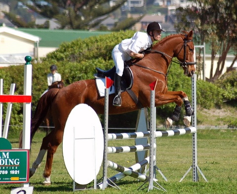
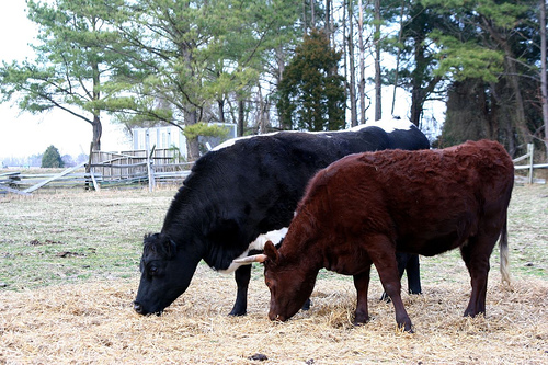
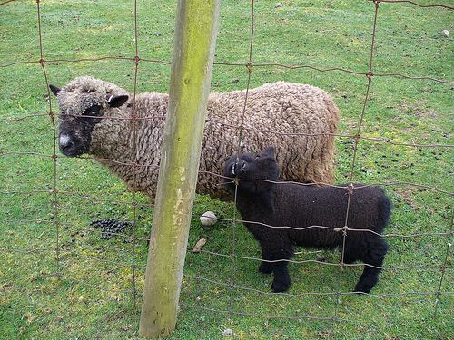
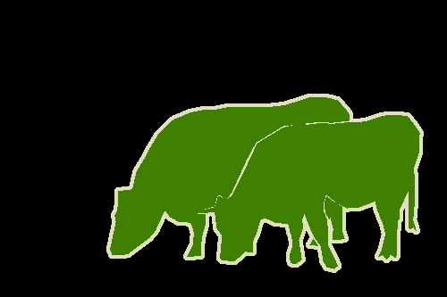
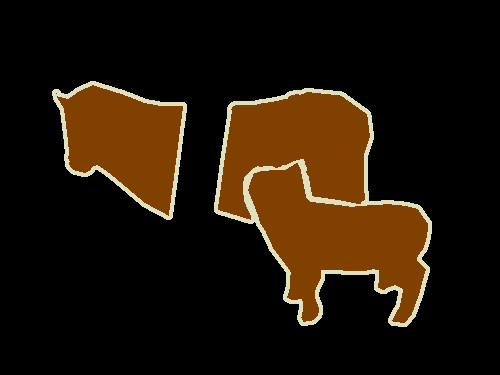
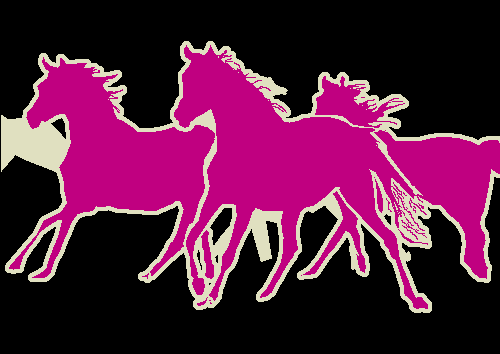
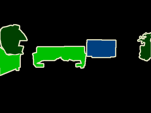
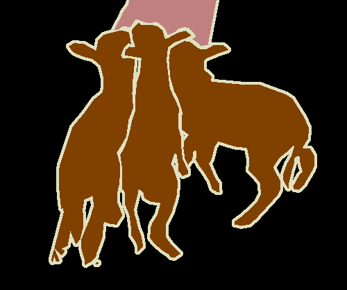
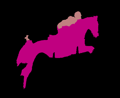
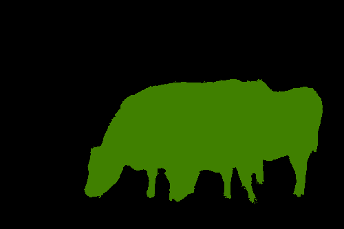
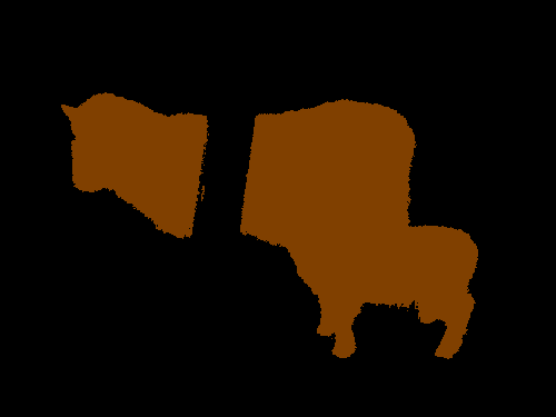
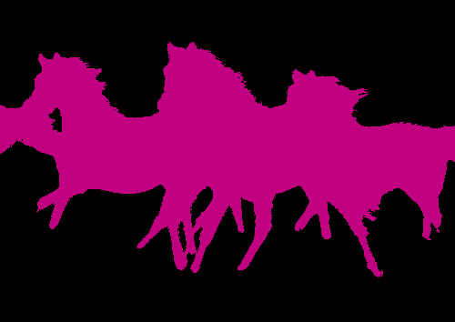
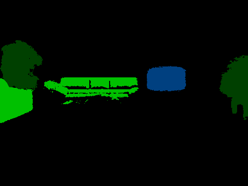
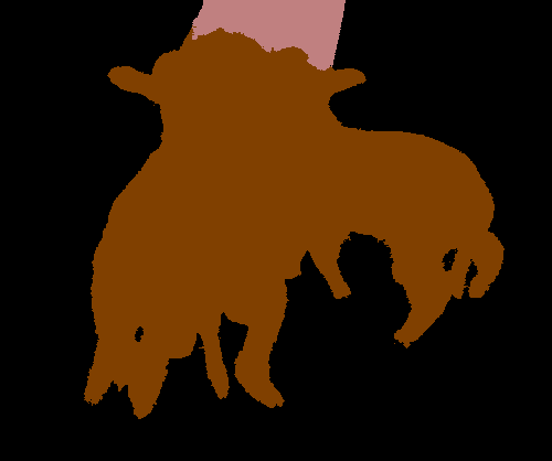
Figure 4: Qualitative segmentation results on the VOC12 validation set. Top: original images. Middle: ground truth with ignored boundary. Bottom: Our results of PMM.

4.4 Failure Case and Remedy

In Fig. 3 we can see that, the details of our pseudo-masks are much better than SEAM with Random Walk. But the mIoU of ours is not very high. The problem is the under-activation CAM, which causes incomplete prediction map or false positive. For this issue, the experiment in Tab. 6 and visualization in Fig. 5 prove that this phenomenon is able to remedy by fully supervised segmentation. Thus PPMG reserves the details, on the other hand, segmentation model remedies the miss area.

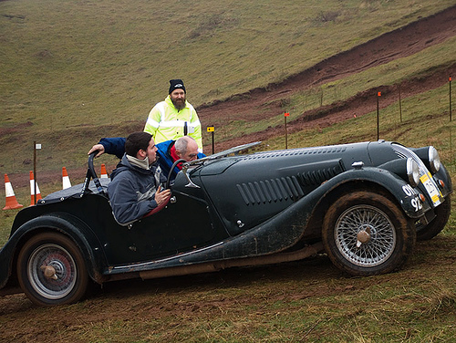
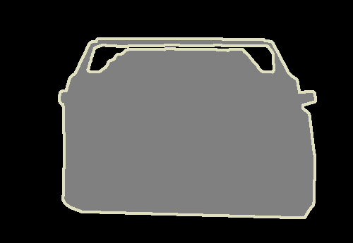
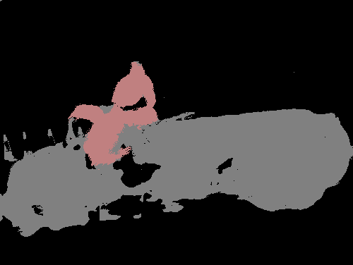
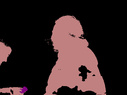
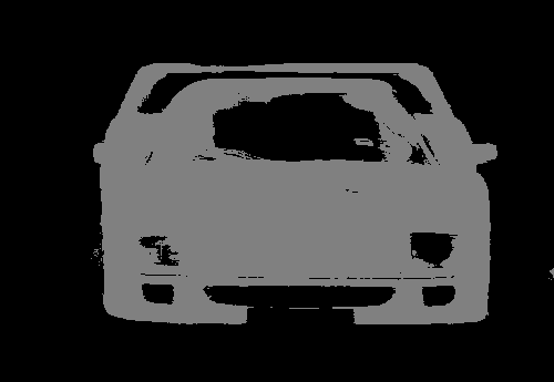
Figure 5: Failure cases of pseudo-masks and its segmentation results on VOC12 validation set. First line: original images. Second line: ground truth. Third line: failure cases of our pseudo-masks. Last line: segmentation remedy results.

5 Conclusion

In weakly supervised semantic segmentation, there are some matters about pseudo-mask in the generation and utilization. To solve these matters, we propose the Proportional Pseudo-mask Generation to identify the category independently and avoid direct score comparison, and the Coefficient of Variation Smoothing to smooth the CAM by its distribution statistics. Then, we add Pretended Under-fitting Strategy to FSSS, and verify the effectiveness of Cyclic Pseudo-mask experimentally. We solve the matters about pseudo-mask and achieves new state-of-the-art in both VOC12 and COCO14 datasets, even beyond the methods using extra information.

6 Acknowledgement

The work is partially supported by Innovation and Technology Commission of the Hong Kong Special Administrative Region, China (Enterprise Support Scheme under the Innovation and Technology Fund B/E030/18).

References

- [1] J. Ahn, S. Cho, and S. Kwak. Weakly supervised learning of instance segmentation with inter-pixel relations. In 2019 IEEE Conference on Computer Vision and Pattern Recognition, pages 2204–2213, 2019.
- [2] Jiwoon Ahn and Suha Kwak. Learning pixel-level semantic affinity with image-level supervision for weakly supervised semantic segmentation. In Proceedings of the IEEE Conference on Computer Vision and Pattern Recognition, pages 4981–4990, 2018.
- [3] Amy Bearman, Olga Russakovsky, Vittorio Ferrari, and Li Fei-Fei. What’s the point: Semantic segmentation with point supervision. In European conference on computer vision, pages 549–565. Springer, 2016.
- [4] Siddhartha Chandra and Iasonas Kokkinos. Fast, exact and multi-scale inference for semantic image segmentation with deep gaussian crfs. In European conference on computer vision, pages 402–418, 2016.
- [5] Yu-Ting Chang, Qiaosong Wang, Wei-Chih Hung, Robinson Piramuthu, Yi-Hsuan Tsai, and Ming-Hsuan Yang. Weakly-supervised semantic segmentation via sub-category exploration. In Proceedings of the IEEE Conference on Computer Vision and Pattern Recognition, pages 8991–9000, 2020.
- [6] Liang-Chieh Chen, George Papandreou, Iasonas Kokkinos, Kevin Murphy, and Alan L. Yuille. Semantic image segmentation with deep convolutional nets and fully connected crfs. In International Conference on Learning Representations, 2015.
- [7] Liang-Chieh Chen, George Papandreou, Iasonas Kokkinos, Kevin Murphy, and Alan L Yuille. Deeplab: Semantic image segmentation with deep convolutional nets, atrous convolution, and fully connected crfs. IEEE transactions on pattern analysis and machine intelligence, 40(4):834–848, 2017.
- [8] MMSegmentation Contributors. Mmsegmentation, an open source semantic segmentation toolbox. https://github.com/open-mmlab/mmsegmentation, 2020.
- [9] Jifeng Dai, Kaiming He, and Jian Sun. Boxsup: Exploiting bounding boxes to supervise convolutional networks for semantic segmentation. In Proceedings of the IEEE international conference on computer vision, pages 1635–1643, 2015.
- [10] Mark Everingham, Luc Van Gool, Christopher KI Williams, John Winn, and Andrew Zisserman. The pascal visual object classes (voc) challenge. International journal of computer vision, 88(2):303–338, 2010.
- [11] Junsong Fan, Zhaoxiang Zhang, Chunfeng Song, and Tieniu Tan. Learning integral objects with intra-class discriminator for weakly-supervised semantic segmentation. In Proceedings of the IEEE Conference on Computer Vision and Pattern Recognition, pages 4283–4292, 2020.
- [12] Bharath Hariharan, Pablo Arbeláez, Lubomir Bourdev, Subhransu Maji, and Jitendra Malik. Semantic contours from inverse detectors. In 2011 International Conference on Computer Vision, pages 991–998. IEEE, 2011.
- [13] Qibin Hou, Peng-Tao Jiang, Yunchao Wei, and Ming-Ming Cheng. Self-erasing network for integral object attention. arXiv preprint arXiv:1810.09821, 2018.
- [14] Zilong Huang, Xinggang Wang, Jiasi Wang, Wenyu Liu, and Jingdong Wang. Weakly-supervised semantic segmentation network with deep seeded region growing. In Proceedings of the IEEE Conference on Computer Vision and Pattern Recognition, pages 7014–7023, 2018.
- [15] Peng-Tao Jiang, Qibin Hou, Yang Cao, Ming-Ming Cheng, Yunchao Wei, and Hong-Kai Xiong. Integral object mining via online attention accumulation. In Proceedings of the IEEE International Conference on Computer Vision, pages 2070–2079, 2019.
- [16] Anna Khoreva, Rodrigo Benenson, Jan Hosang, Matthias Hein, and Bernt Schiele. Simple does it: Weakly supervised instance and semantic segmentation. In Proceedings of the IEEE Conference on Computer Vision and Pattern Recognition, July 2017.
- [17] Alexander Kolesnikov and Christoph H Lampert. Seed, expand and constrain: Three principles for weakly-supervised image segmentation. In European conference on computer vision, pages 695–711. Springer, 2016.
- [18] Philipp Krähenbühl and Vladlen Koltun. Efficient inference in fully connected crfs with gaussian edge potentials. In J. Shawe-Taylor, R. Zemel, P. Bartlett, F. Pereira, and K. Q. Weinberger, editors, Advances in Neural Information Processing Systems, volume 24, pages 109–117. Curran Associates, Inc., 2011.
- [19] Alex Krizhevsky, Ilya Sutskever, and Geoffrey E Hinton. Imagenet classification with deep convolutional neural networks. Advances in neural information processing systems, 25:1097–1105, 2012.
- [20] Jungbeom Lee, Eunji Kim, Sungmin Lee, Jangho Lee, and Sungroh Yoon. Ficklenet: Weakly and semi-supervised semantic image segmentation using stochastic inference. In Proceedings of the IEEE Conference on Computer Vision and Pattern Recognition, pages 5267–5276, 2019.
- [21] Xueyi Li, Tianfei Zhou, Jianwu Li, Yi Zhou, and Zhaoxiang Zhang. Group-wise semantic mining for weakly supervised semantic segmentation. arXiv preprint arXiv:2012.05007, 2020.
- [22] Yi Li, Zhanghui Kuang, Yimin Chen, and Wayne Zhang. Data-driven neuron allocation for scale aggregation networks. In Proceedings of the IEEE Conference on Computer Vision and Pattern Recognition, pages 11526–11534, 2019.
- [23] Di Lin, Jifeng Dai, Jiaya Jia, Kaiming He, and Jian Sun. Scribblesup: Scribble-supervised convolutional networks for semantic segmentation. In Proceedings of the IEEE conference on computer vision and pattern recognition, pages 3159–3167, 2016.
- [24] Tsung-Yi Lin, Michael Maire, Serge Belongie, James Hays, Pietro Perona, Deva Ramanan, Piotr Dollár, and C Lawrence Zitnick. Microsoft coco: Common objects in context. In European conference on computer vision, pages 740–755. Springer, 2014.
- [25] Yun Liu, Yu-Huan Wu, Pei-Song Wen, Yu-Jun Shi, Yu Qiu, and Ming-Ming Cheng. Leveraging instance-, image-and dataset-level information for weakly supervised instance segmentation. IEEE Transactions on Pattern Analysis and Machine Intelligence, 2020.
- [26] Ziwei Liu, Xiaoxiao Li, Ping Luo, Chen-Change Loy, and Xiaoou Tang. Semantic image segmentation via deep parsing network. In 2015 IEEE International Conference on Computer Vision, pages 1377–1385, 2015.
- [27] Deepak Pathak, Philipp Krahenbuhl, and Trevor Darrell. Constrained convolutional neural networks for weakly supervised segmentation. In Proceedings of the IEEE international conference on computer vision, pages 1796–1804, 2015.
- [28] Pedro O Pinheiro and Ronan Collobert. From image-level to pixel-level labeling with convolutional networks. In Proceedings of the IEEE conference on computer vision and pattern recognition, pages 1713–1721, 2015.
- [29] Fatemehsadat Saleh, Mohammad Sadegh Aliakbarian, Mathieu Salzmann, Lars Petersson, Stephen Gould, and Jose M Alvarez. Built-in foreground/background prior for weakly-supervised semantic segmentation. In European conference on computer vision, pages 413–432. Springer, 2016.
- [30] Wataru Shimoda and Keiji Yanai. Self-supervised difference detection for weakly-supervised semantic segmentation. In Proceedings of the IEEE International Conference on Computer Vision, pages 5208–5217, 2019.
- [31] Guolei Sun, Wenguan Wang, Jifeng Dai, and Luc Van Gool. Mining cross-image semantics for weakly supervised semantic segmentation. In European Conference on Computer Vision, pages 347–365. Springer, 2020.
- [32] Meng Tang, Abdelaziz Djelouah, Federico Perazzi, Yuri Boykov, and Christopher Schroers. Normalized cut loss for weakly-supervised cnn segmentation. In Proceedings of the IEEE Conference on Computer Vision and Pattern Recognition, June 2018.
- [33] Yude Wang, Jie Zhang, Meina Kan, Shiguang Shan, and Xilin Chen. Self-supervised equivariant attention mechanism for weakly supervised semantic segmentation. In Proceedings of the IEEE Conference on Computer Vision and Pattern Recognition, June 2020.
- [34] Yunchao Wei, Huaxin Xiao, Honghui Shi, Zequn Jie, Jiashi Feng, and Thomas S Huang. Revisiting dilated convolution: A simple approach for weakly-and semi-supervised semantic segmentation. In Proceedings of the IEEE Conference on Computer Vision and Pattern Recognition, pages 7268–7277, 2018.
- [35] Zifeng Wu, Chunhua Shen, and Anton Van Den Hengel. Wider or deeper: Revisiting the resnet model for visual recognition. Pattern Recognition, 90:119–133, 2019.
- [36] Jia Xu, Alexander G. Schwing, and Raquel Urtasun. Learning to segment under various forms of weak supervision. In Proceedings of the IEEE Conference on Computer Vision and Pattern Recognition, June 2015.
- [37] Qi Yao and Xiaojin Gong. Saliency guided self-attention network for weakly and semi-supervised semantic segmentation. IEEE Access, 8:14413–14423, 2020.
- [38] Yu Zeng, Yunzhi Zhuge, Huchuan Lu, and Lihe Zhang. Joint learning of saliency detection and weakly supervised semantic segmentation. In Proceedings of the IEEE International Conference on Computer Vision, pages 7223–7233, 2019.
- [39] Dong Zhang, Hanwang Zhang, Jinhui Tang, Xiansheng Hua, and Qianru Sun. Causal intervention for weakly-supervised semantic segmentation. arXiv preprint arXiv:2009.12547, 2020.
- [40] Hengshuang Zhao, Jianping Shi, Xiaojuan Qi, Xiaogang Wang, and Jiaya Jia. Pyramid scene parsing network. In Proceedings of the IEEE conference on computer vision and pattern recognition, pages 2881–2890, 2017.
- [41] Shuai Zheng, Sadeep Jayasumana, Bernardino Romera-Paredes, Vibhav Vineet, Zhizhong Su, Dalong Du, Chang Huang, and Philip H. S. Torr. Conditional random fields as recurrent neural networks. In 2015 IEEE International Conference on Computer Vision, pages 1529–1537, 2015.
- [42] Bolei Zhou, Aditya Khosla, Agata Lapedriza, Aude Oliva, and Antonio Torralba. Learning deep features for discriminative localization. In Proceedings of the IEEE conference on computer vision and pattern recognition, pages 2921–2929, 2016.