Partially Explicit Time Discretization for Time Fractional Diffusion Equation

Abstract

Time fractional PDEs have been used in many applications for modeling and simulations. Many of these applications are multiscale and contain high contrast variations in the media properties. It requires very small time step size to perform detailed computations. On the other hand, in the presence of small spatial grids, very small time step size is required for explicit methods. Explicit methods have many advantages as we discuss in the paper. In this paper, we propose a partial explicit method for time fractional PDEs. The approach solves the forward problem on a coarse computational grid, which is much larger than spatial heterogeneities, and requires only a few degrees of freedom to be treated implicitly. Via the construction of appropriate spaces and careful stability analysis, we can show that the time step can be chosen not to depend on the contrast or scale as the coarse mesh size. Thus, one can use larger time step size in an explicit approach. We present stability theory for our proposed method and our numerical results confirm the stability findings and demonstrate the performance of the approach.

1 Introduction

Many problems have multiscale nature. These include flow in porous media, composite materials and so on. Multiscale features typically occur spatially due to variable nature of media properties. For example, porous media properties can vary at different scales. Many multiscale methods have been developed for steady state and dynamic problems. However, there has been limited research on multiscale methods with fractional time derivatives. Fractional time derivatives occur in many applications as will be discussed next.

Recently, there has been many research activities related to equations with fractional derivatives. This is due to the numerous effective applications of fractional calculus in various fields of science and technology [1, 23, 36, 38]. For example, fractional derivatives are used for describing the physical process of statistical transfer and this leads to diffusion equations of fractional orders [6, 35]. Many methods have been developed for the numerical solution of time fractional equations. The most common differential approximation of the time fractional derivative is the so-called L1 method [36, 45]. To approximate the time fractional derivative with a higher order of accuracy, difference analogs of the L2 type are used [2, 3, 20]. The basic properties of these difference analogs are well studied and are used for solving various fractional PDEs. In this paper, we combine time fractional PDE approximation with multiscale splitting to solve challenging time fractional PDEs in heterogeneous media.

For time fractional PDEs, it is difficult to use explicit methods due to time step constraints. The time step constraints involve the fractional power and the fine grid which is much smaller compared to the coarse grid and thus one requires smaller time step size for explicit methods as the fractional power gets smaller. In the presence of multiscale features, the time step size is even smaller as the contrast increases.

In this paper, we propose partially explicit approach, where one implicitly treats a few degrees of freedom defined on a coarse grid and the rest of degrees of freedom are treated explicitly. This approach allows removing the time step constraint due to the contrast and reduce the time step constraint due to the fine-grid mesh size. In particular, the time step size is smaller than an appropriate fractional power of coarse-grid mesh size. In general, by choosing coarse-grid mesh size larger, one can allieviate this problem and make the time step larger. We would like to note that explicit methods have many advantages as they provide less communications and easy to compute. They can also be used in constructing efficient neural network architectures.

In the paper, we present a novel framework for stability analysis of implicit-explicit methods for time fractional PDEs. The stability analysis starts with a space decomposition for coarse-grid degrees of freedom and the other degrees of freedom. This framework derives conditions necessary for partial explicit schemes to be stable. In particular, the stability conditions show that one needs the second space to be free of contrast. To achieve this, we need spaces like CEM-GMsFEM, which we describe next.

In previous findings, many multiscale algorithms have been developed, such as RVE based homogenization approaches [17, 32], multiscale finite element methods [17, 24, 29], generalized multiscale finite element methods (GMsFEM) [7, 8, 9, 12, 16], constraint energy minimizing GMsFEM (CEM-GMsFEM) [10, 11], nonlocal multi-continua (NLMC) approaches [14], metric-based upscaling [37], heterogeneous multiscale method [15], localized orthogonal decomposition (LOD) [22], equation-free approaches [40, 41], multiscale stochastic approaches [25, 26, 27], and hierarchical multiscale method [4], are developed to address spatial heterogeneities. For high-contrast problems, approaches that require multiple multiscale basis functions are needed, which include approaches such as GMsFEM and NLMC [10, 11, 14]. We also note some works on numerical homogenization of time fractional PDEs [28, 5]. Special constructions are needed for computing multiscale basis functions. These spaces satisfy the conditions needed for partial explicit methods.

Splitting approaches are used for many applications, [34, 44]. For example, they are used for splitting physics. In our recent works, we have used splitting approaches in a design of partial explicit methods for parabolic and wave equations [18, 19]. In the current paper, we extend these ideas to time fractional diffusion equations, which require significant modifications.

We present several numerical results, where we compare our proposed approaches with the approaches where all degrees of freedom are treated implicitly. We consider high contrast permeability fields. Our numerical results show that the proposed methods provide similar accuracy compared to the methods where all degrees of freedom are treated implicitly. In conclusion, we would like to highlight some novelties of the proposed methods.

• The proposed methods provide a venue for performing partial explicit time stepping for time fractional PDEs, where time step constraints can be severe.

• The time step constraint depends on the coarse mesh size and is independent of the contrast.

• Numerical results confirm our theoretical findings.

The paper is organized as follows. In the next section, we present some preliminaries. Section 3 is devoted to stability conditions and their derivations. In Section 4, we briefly present the construction of spaces for partially explicit method. We present the numerical results in Section 5 and conclude the paper in Section 6.

2 Preliminaries

Let $\Omega$ be a bounded domain in $\mathbb{R}^{d}\,(d=1,2,3)$ with a sufficiently smooth boundary $\partial\Omega$. We consider a partial differential equation with the fractional derivative in time $t$, satisfying:

$$\left\{\begin{aligned} \partial_{t}^{\alpha}u(x,t)&=\nabla\cdot\left(\kappa({x})\nabla u(x,t)\right)+f(x,t)&&\text{in }\Omega,\quad t\in\left(0,T\right]\\ u&=0&&\text{on }\partial\Omega,\;t\in\left(0,T\right]\\ u(0)&=u_{0}(x)&&\text{in }\Omega.\end{aligned}\right.$$ (1)

Here, $0<\alpha<1$ is a given fixed parameter. $\kappa(x)$ is a high-contrast multiscale field. The initial function $u_{0}$ is a given term and $T>0$ is a fixed value. The source term $f$ satisfies $t^{1-\alpha}f\in L^{1}(0,T;L^{2}(\Omega))$.

In the model problem (1), $\partial_{t}^{\alpha}w$ refers to the left-sided Caputo fractional derivative of order $\alpha$ of the function $w(t)$, defined by (see, e.g. [30, p. 91, (2.4.1)] or [39, p. 78])

$$\partial^{\alpha}_{t}w(t)=\frac{1}{\Gamma(1-\alpha)}\int_{0}^{t}\frac{1}{(t-s)^{\alpha}}w^{\prime}(s)ds.$$

The fractional diffusion equations were introduced in physics aiming at describing diffusions in media with fractal geometry [35]. They are enormously applied to many fields, for example in engineering, physics, biology and finance. Their practical applications include electron transport in Xerox photocopier, visco-elastic materials, and protein transport in cell membrane [42, 21, 31].

To discretize the model problem (1), we first decompose the time domain $[0,T]$ into $N$ time subdomains $(T_{n},T_{n+1})$, $n=0,1,\cdots,N-1$, with $0=T_{0}<T_{1}<\cdots<T_{N-1}<T_{N}=T$ and $\Delta T_{n}:=T_{n+1}-T_{n}$. For simplicity, we assume $\Delta T_{n}=\Delta T$ for any $n=0,1,\cdots,N-1$. Let $\mathcal{T}_{H}$ be a decomposition of the spatial domain $\Omega$ into non-overlapping shape-regular rectangular elements with maximal mesh size $H$. Let $\mathcal{T}^{h}$ be a refinement of $\mathcal{T}^{H}$ with $h\ll H$. One could choose a finite element space $V_{h}\subset H_{0}^{1}(\Omega)$ with $h$ being an extremely small number and utilize full discretization to solve (1). For the sake of saving computational cost, we would like to construct a finite dimensional space $V_{H}\subset H_{0}^{1}(\Omega)$ based on $\mathcal{T}_{H}$.

Utilizing finite difference approximation to discretize the time-fractional derivative [33], one obtains the following approximation

$$\partial_{t}^{\alpha}u(x,T_{k})\approx\frac{1}{\Gamma(2-\alpha)}\sum_{j=0}^{k}\frac{u(x,T_{k+1-j}-u(x,T_{k-j}))}{\Delta T^{\alpha}}[(j+1)^{1-\alpha}-j^{1-\alpha}],\text{ for }k=1,2,\cdots,N.$$ (2)

Using the implicit Euler scheme and the approximation (2), one obtains the full discretized finite element method which reads as follows: for any $k=0,1,\cdots,N-1$, find $u^{k+1}\in V_{H}$ such that

$$(u^{k+1},v)+\alpha_{0}a(u^{k+1},v)=(1-b_{1})(u^{k},v)+\sum_{j=1}^{k-1}(u^{k-j},v)+b_{k}(u^{0},v)+\alpha_{0}(f^{k+1},v),\leavevmode\nobreak\ \forall v\in V_{H}.$$ (3)

Here, $\alpha_{0}=\Gamma(2-\alpha)\Delta T^{\alpha}$, $a(v,w):=(\kappa\nabla v,\nabla w)$ for any $v,w\in V_{H}$ and $b_{j}=(j+1)^{1-\alpha}-j^{1-\alpha}$, for $j=0,1,\cdots,k$. We remark that $u^{k}$ is an approximation to the solution $u(T^{k})$.

Next, we clarify some notations used throughout the article. We write $(\cdot,\cdot)$ to denote the inner product in $L^{2}(\Omega)$ and $\left\|\cdot\right\|$ for the corresponding norm. Let $H^{1}(\Omega)$ be the classical Sobolev space with the norm $\left\|v\right\|_{1}:=\left(\left\|v\right\|^{2}+\left\|\nabla v\right\|^{2}\right)^{1/2}$ for any $v\in H^{1}(\Omega)$ and $H_{0}^{1}(\Omega)$ the subspace of functions having a vanishing trace. For any subset $S\subset\Omega$, we denote $V(S):=H_{0}^{1}(S)$. We use $\left\|\cdot\right\|_{a}$ to denote the norm induced by the $a$-norm. That is, $\left\|v\right\|_{a}=\sqrt{a(v,v)}$.

3 Three Schemes and Stabilities

In this section, we will prove the unconditional stability for implicit Euler scheme in Subsection 3.1. In Subsection 3.2, we establish the stability condition for the explicit Euler scheme. Finally, in Subsection 3.3, we introduce a partial splitting algorithm and discuss the stability condition for the algorithm.

3.1 Stability of Implicit Euler Scheme

We present in the following theorem that the implicit Euler scheme is unconditionally stable (cf. [43]).

Theorem 3.1.

Assume the source term $f$ satisfies $t^{1-\alpha}f\in L^{1}(0,T;L^{2}(\Omega))$. Let $\Delta T$ be the time step size and define $\alpha_{0}:=\Gamma(2-\alpha)\Delta T^{\alpha}$. Let $u^{k}$ be the solution to (3) for $k=1,2,\cdots,N$. Then the implicit Euler Scheme (3) is unconditionally stable. Moreover, we have the following stability estimate:

$$\left\|u^{N}\right\|^{2}_{a}\leq\left\|u^{0}\right\|_{a}^{2}+\alpha_{0}\sum_{k=0}^{N-1}\left\|f^{k+1}\right\|^{2}.$$

Proof.

Note that (3) can be rewritten into

$$\sum_{j=0}^{k}b_{k-j}\big{(}u^{j+1}-u^{j},v\big{)}+\alpha_{0}(\kappa\nabla u^{k+1},\nabla v)=\alpha_{0}(f^{k+1},v)\leavevmode\nobreak\ \forall v\in V_{H}.$$ (4)

Define $b_{k}:=b_{-k}$ for any $k<0$ and $k\in\mathbb{Z}$. Choosing $v=u^{k+1}-u^{k}$ in (4) and taking a summation over $k$ from $0$ to $N-1$, one obtains the following equality.

$$\sum_{k=0}^{N-1}\sum_{j=0}^{k}b_{k-j}\big{(}u^{j+1}-u^{j},u^{k+1}-u^{k}\big{)}+\alpha_{0}\sum_{k=0}^{N-1}a(u^{k+1},u^{k+1}-u^{k})=\sum_{k=0}^{N-1}\alpha_{0}(f^{k+1},u^{k+1}-u^{k}).$$ (5)

Notice that the first term of (5) can be written as

$$\sum_{k=0}^{N-1}\sum_{j=0}^{k}b_{k-j}\big{(}u^{j+1}-u^{j},u^{k+1}-u^{k}\big{)}=\frac{b_{0}}{2}\sum_{k=0}^{N-1}\left\|u^{k+1}-u^{k}\right\|^{2}+\frac{1}{2}\sum_{k=0}^{N-1}\sum_{j=0}^{N-1}b_{|k-j|}(u^{j+1}-u^{j},u^{k+1}-u^{k}).$$

Recall that

$$b_{k}=(k+1)^{1-\alpha}-k^{1-\alpha}=\frac{1}{1-\alpha}\int_{0}^{1}(k+s)^{-\alpha}ds.$$

Notice that $\phi(k)=(k+s)^{-\alpha}$ is a complete monotonic function. It follows from Hausdorff-Bernstein-Widder Theorem that $(k+s)^{-\alpha}=\int_{0}^{\infty}e^{-k\tau}dg_{s}(\tau)$ for some cumulative distribution function $g_{s}$. We then have

$$\sum_{k=0}^{N-1}\sum_{j=0}^{N-1}b_{|k-j|}(u^{j+1}-u^{j},u^{k+1}-u^{k})$$

$$= \frac{1}{1-\alpha}\int_{0}^{1}\int_{0}^{\infty}\sum_{k=0}^{N-1}\sum_{j=0}^{N-1}e^{-|k-j|\tau}(u^{j+1}-u^{j})(u^{k+1}-u^{k})dg_{s}(\tau)ds.$$

Create a matrix $M$ of size $N\times N$ with entry $M_{k,j}=e^{-|k-j|t}$ for $0\leq k,j\leq N-1$. Then the matrix $M$ is positive definite for $t>0$. Therefore,

$$\sum_{k=0}^{N-1}\sum_{j=0}^{N-1}b_{|k-j|}(u^{j+1}-u^{j}),u^{k+1}-u^{k})>0.$$

Therefore, we have

$$\sum_{k=0}^{N-1}\sum_{j=0}^{k}b_{k-j}\big{(}u^{j+1}-u^{j},u^{k+1}-u^{k}\big{)}+\alpha_{0}\sum_{k=0}^{N-1}a(u^{k+1},u^{k+1}-u^{k})\geq\frac{1}{2}\sum_{k=0}^{N-1}\left\|u^{k+1}-u^{k}\right\|^{2}+\alpha_{0}\sum_{k=0}^{N-1}a(u^{k+1},u^{k+1}-u^{k}).$$

Notice that $a(u^{k+1},u^{k+1}-u^{k})=\frac{1}{2}(\left\|u^{k+1}\right\|^{2}_{a}-\left\|u^{k}\right\|^{2}_{a}+\left\|u^{k+1}-u^{k}\right\|^{2}_{a})$. Furthermore, utilizing Cauchy-Schwartz Inequality, one obtains the following estimate.

$$\alpha_{0}\sum_{k=0}^{N-1}(f^{k+1},u^{k+1}-u^{k}) \leq\sum_{k=0}^{N-1}\alpha_{0}\left\|f^{k+1}\right\|\left\|u^{k+1}-u^{k}\right\|$$ (6)

$$\leq\frac{\alpha_{0}^{2}}{2}\sum_{k=0}^{N-1}\left\|f^{k+1}\right\|^{2}+\frac{1}{2}\sum_{k=0}^{N-1}\left\|u^{k+1}-u^{k}\right\|^{2}$$ (7)

Therefore we have $\frac{1}{2}\sum_{k=0}^{N-1}\left\|u^{k+1}-u^{k}\right\|^{2}+\sum_{k=0}^{N-1}\frac{\alpha_{0}}{2}(\left\|u^{k+1}\right\|^{2}_{a}-\left\|u^{k}\right\|^{2}_{a}+\left\|u^{k+1}-u^{k}\right\|^{2}_{a})\leq\frac{\alpha_{0}^{2}}{2}\sum_{k=0}^{N-1}\left\|f^{k+1}\right\|^{2}+\frac{1}{2}\sum_{k=0}^{N-1}\left\|u^{k+1}-u^{k}\right\|^{2}.$ It follows from $f$ satisfies $t^{1-\alpha}f\in L^{1}(0,T;L^{2}(\Omega))$ that $\alpha_{0}\sum_{k=0}^{N-1}\left\|f^{k+1}\right\|^{2}$ is bounded. So we have

$$\left\|u^{N}\right\|^{2}_{a}\leq\left\|u^{0}\right\|_{a}^{2}+\alpha_{0}\sum_{k=0}^{N-1}\left\|f^{k+1}\right\|^{2}.$$ (8)

∎

3.2 Stability of Explicit Euler Scheme

With explicit Euler scheme and the approximation (2), the full discretized finite element method reads as follows: for any $k=0,1,\cdots,N-1$, find $u^{k+1}\in V_{H}$ such that

$$(u^{k+1},v)+\alpha_{0}a(u^{k},v)=(1-b_{1})(u^{k},v)+\sum_{j=1}^{k-1}(u^{k-j},v)+b_{k}(u^{0},v)+\alpha_{0}(f^{k+1},v),\leavevmode\nobreak\ \forall v\in V_{H}.$$ (9)

By a similar argument and $a(u^{k},u^{k+1}-u^{k})=\frac{1}{2}(\left\|u^{k+1}\right\|_{a}^{2}-\left\|u^{k}\right\|_{a}^{2}-\left\|u^{k+1}-u^{k}\right\|_{a}^{2})$, we present the stability condition of explicit Euler scheme in the following theorem. For the brevity of the paper, we omit the proof here.

Theorem 3.2.

Assume the source term $f$ satisfies $t^{1-\alpha}f\in L^{1}(0,T;L^{2}(\Omega))$. Let $\Delta T$ be the time step size and define $\alpha_{0}:=\Gamma(2-\alpha)\Delta T^{\alpha}$. Let $u^{k}$ be the solution to (9) for $k=1,2,\cdots,N$. Then the explicit scheme (9) is stable if $\left\|v\right\|^{2}\geq 2\alpha_{0}\left\|v\right\|_{a}^{2}$ for any $v\in V_{H}$. Moreover, we have the following estimate

$$\left\|u^{N}\right\|_{a}^{2}\leq\left\|u^{0}\right\|_{a}^{2}+\alpha_{0}\sum_{k=0}^{N-1}\left\|f^{k+1}\right\|^{2}.$$ (10)

3.3 Stability of Partially Explicit Scheme

In this subsection, we shall introduce a partially explicit temporal splitting scheme. For this purpose, we decompose the solution space $V_{H}$ into two subspaces $V_{H,1}$ and $V_{H,2}$. That is, $V_{H}=V_{H,1}+V_{H,2}$. Then the solution $u^{k+1}$ can be written as $u^{k+1}=u^{k+1}_{1}+u^{k+1}_{2}$ with $u^{k+1}_{1}\in V_{H,1}$ and $u^{k+1}_{2}\in V_{H,2}$. The full discretized finite element method with partially explicit temporal splitting scheme reads as follows: for any $k=0,1,\cdots,N-1$, find $u^{k+1}_{1}\in V_{H,1}$ and $u^{k+1}_{2}\in V_{H,2}$ such that

$$(u^{k+1},v)+\alpha_{0}a(u^{k+1}_{1}+u^{k}_{2},v)=(1-b_{1})(u^{k},v)+\sum_{j=1}^{k-1}(u^{k-j},v)+b_{k}(u^{0},v)+\alpha_{0}(f^{k+1},v),\leavevmode\nobreak\ \forall v\in V_{H}.$$ (11)

We study the stability of the partially explicit scheme in the following theorem.

Theorem 3.3.

Assume the source term $f$ satisfies $t^{1-\alpha}f\in L^{1}(0,T;L^{2}(\Omega))$. Let $\Delta T$ be the time step size and define $\alpha_{0}:=\Gamma(2-\alpha)\Delta T^{\alpha}$. Let $u^{k}$ be the solution to (11) for $k=1,2,\cdots,N$. Then the partially explicit scheme (11) is stable if

$$\left\|u_{1}+u_{2}\right\|^{2}\geq 2(1-\gamma^{2})\left\|u_{2}\right\|^{2}\text{ for any }u_{1}\in V_{H,1},u_{2}\in V_{H,2}$$ (12)

and

$$\left\|v\right\|\geq\alpha_{0}(1-\gamma^{2})^{-1}\left\|v\right\|_{a}^{2}\text{ for any }v\in V_{H,2},$$ (13)

for some constant $\gamma\in[0,1)$. Furthermore, we have the following estimate

$$\left\|u^{N}\right\|_{a}^{2}\leq\left\|u^{0}\right\|_{a}^{2}+\sum_{k=0}^{N-1}\alpha_{0}\left\|f^{k+1}\right\|^{2}.$$ (14)

Proof.

Notice that

$$a(u^{k+1}_{1}-u^{k}_{2},u^{k+1}-u^{k}) =a(u^{k+1},u^{k+1}-u^{k})+a(u^{k}_{2}-u^{k+1}_{2},u^{k+1}-u^{k})$$

$$\geq\frac{1}{2}(\left\|u^{k+1}\right\|_{a}^{2}-\left\|u^{k}\right\|_{a}^{2}-\left\|u^{k+1}-u^{k}\right\|_{a}^{2})-\frac{1}{2}(\left\|u^{k+1}_{2}-u^{k}_{2}\right\|_{a}^{2}+\left\|u^{k+1}-u^{k}\right\|_{a}^{2})$$

$$=\frac{1}{2}(\left\|u^{k+1}\right\|_{a}^{2}-\left\|u^{k}\right\|_{a}^{2}-\left\|u^{k+1}_{2}-u^{k}_{2}\right\|_{a}^{2}).$$

Applying a similar argument adopted in the proof of Theorem 3.1 and combining (12) and (13), we have

$$\left\|u^{N}\right\|_{a}^{2}\leq\left\|u^{0}\right\|_{a}^{2}+\sum_{k=0}^{N-1}\alpha_{0}\left\|f^{k+1}\right\|^{2}.$$ (15)

∎

4 $V_{H,1}$ and $V_{H,2}$ Constructions

In this section, we shall introduce a possible way to construct spaces $V_{H,1}$ and $V_{H,2}$ such that the partially explicit scheme is stable. Our construction follows our previous work [13]. We will first recap the constrained energy minimization (CEM) finite element method and show that the CEM type finite element space is a good choice of $V_{H,1}$ since the CEM multiscale basis functions are constructed in a way that they are almost orthogonal to the space $\tilde{V}$ which will be defined in Section 4.1. We will present two possible ways of constructing the subspace $V_{H,2}$. Before that, we introduce a concept called oversampling domain, which will be used later. For each coarse element $K_{i}$, we define the oversampled region $K_{i,k_{i}}\subseteq\Omega$ by enlarging $K_{i}$ by $k_{i}\in\mathbb{N}$ layer(s), i.e.,

$$K_{i,0}:=K_{i},\quad K_{i,k_{i}}:=\bigcup\{K\in\mathcal{T}^{H}:K\cap K_{i,k_{i}-1}\neq\emptyset\}\quad\text{for }k_{i}=1,2,\cdots.$$

We call $k_{i}$ a parameter of oversampling related to the coarse element $K_{i}$. See Figure 1 for an illustration of $K_{i,1}$. For simplicity, we denote $K_{i}^{+}$ a generic oversampling region related to the coarse element $K_{i}$ with a specific oversampling parameter $k_{i}$.

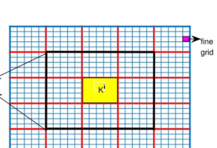
Figure 1: Illustration of the oversampling domain.

4.1 CEM method

In this section, we will discuss the CEM method for solving the problem (3). In particular, we will focus on constructing the finite element space by solving a constrained energy minimization problem. Let $\mathcal{T}_{H}$ be a decomposition of the spatial domain $\Omega$ into non-overlapping shape-regular rectangular elements with maximal mesh size $H$. We shall construct a finite dimensional space $V_{H}\subset H_{0}^{1}(\Omega)$. For each element $K_{i}\in\mathcal{T}_{H}$, one obtains a set of auxiliary basis functions $\{\psi_{j}^{(i)}\}_{j=1}^{L_{i}}\subset V(K_{j})$ by solving eigenvalue problems: finding $(\lambda_{j}^{(i)},\psi_{j}^{(i)})\in\mathbb{R}\times V(K_{j})$ such that

$$\int_{K_{i}}\kappa\nabla\psi_{j}^{i}\cdot\nabla v=\lambda_{j}^{i}s_{i}(\psi_{j}^{i},v),\leavevmode\nobreak\ \leavevmode\nobreak\ \forall v\in V(K_{i}),$$

where $s_{i}(u,v)=\int_{K_{i}}\tilde{\kappa}uv$ and $\tilde{\kappa}=\kappa\sum_{i=1}^{N_{c}}|\nabla\chi_{i}|^{2}$ with $\{\chi_{i}\}_{i=1}^{N_{c}}$ being the standard multiscale finite element basis functions. Select the first $L_{i}$ eigenfunctions corresponding to the first small eigenvalues. $\{\psi_{j}^{(i)}\}_{j=1}^{L_{i}}$ is the set of the auxiliary basis functions and we denote $V_{aux}^{(i)}:=\text{span}\{\psi_{j}^{(i)}:\;1\leq j\leq L_{i}$ as the local auxiliary space. We then can define a local projection operator $\Pi_{K_{i}}:L^{2}(K_{i})\mapsto V_{aux}^{(i)}\subset L^{2}(K_{i})$ such that

$$s_{i}(\Pi_{i}u,v)=s_{i}(u,v)\;\forall v\in V_{aux}^{(i)}.$$

Next we define a global projection operator by $\Pi:L^{2}(\Omega)\mapsto V_{aux}\subset L^{2}(\Omega)$ such that

$$s(\Pi u,v)=s(u,v)\;\forall v\in V_{aux}:=\bigcup_{i=1}^{N_{e}}V_{aux}^{(i)},$$

where $s(u,v):=\sum_{i=1}^{N_{e}}s_{i}(u|_{K_{i}},v|_{K_{i}})$ and $N_{e}$ is the number of coarse elements. For each auxiliary basis functions $\psi_{j}^{(i)}$, we can define a local basis function $\phi_{j}^{(i)}\in V(K_{i}^{+})$ such that

$$a(\phi_{j}^{(i)},v)+s(\mu_{j}^{(i)},v) =0 \forall v\in V(K_{i}^{+})$$

$$s(\phi_{j}^{(i)},\nu) =s(\psi_{j}^{(i)},\nu) \forall\nu\in V_{aux}(K_{i}^{+}).$$

We then define the space $V_{cem}$ as

$$V_{cem} :=\text{span}\{\phi_{j}^{(i)}:\;1\leq i\leq N_{e},1\leq j\leq L_{i}\}.$$

The CEM solution $u^{k+1}_{cem}$ for $k=1,2,\cdots,N-1$ is given by

$$(u_{cem}^{k+1},v)+\alpha_{0}a(u_{cem}^{k+1},v)=(1-b_{1})(u_{cem}^{k},v)+\sum_{j=1}^{k-1}(u_{cem}^{k-j},v)+b_{k}(u_{cem}^{0},v)+\alpha_{0}(f^{k+1},v),\leavevmode\nobreak\ \forall v\in V_{cem}.$$ (16)

Now we construct global basis functions $\phi_{j,glo}^{(i)}$. For each auxiliary basis functions $\psi_{j}^{(i)}$, we find $\phi_{j,glo}^{(i)}\in V$ such that

$$a(\phi_{j,glo}^{(i)},v)+s(\mu_{j}^{(i)},v) =0 \forall v\in V$$

$$s(\phi_{j,glo}^{(i)},\nu) =s(\psi_{j,glo}^{(i)},\nu) \forall\nu\in V_{aux}.$$

We remark here that the local multiscale basis $\phi_{j}^{(i)}$ is an approximation of the global basis function $\phi_{j,glo}^{(i)}$. Denote $V_{glo}:=\text{span}\{\phi_{j,glo}^{(i)}:\;1\leq i\leq N_{e},1\leq j\leq L_{i}\}.$ It can be proved the $V_{glo}$ is $a-$orthogonal to a space $\tilde{V}:=\{v\in V:\;\Pi(v)=0\}$. We also know that $V_{cem}$ is closed in $V_{glo}$ and therefore it is almost orthogonal to $\tilde{V}$. Thus, we can choose $V_{cem}$ to be $V_{H,1}$ and it remains to construct a space $V_{H,2}$ in $\tilde{V}$.

4.2 Construction of $V_{H,2}$

In this subsection, we will discuss a choice for the space $V_{H,2}\subset\tilde{V}$. This choice of $V_{H,2}$ is based on the CEM type multiscale finite element space. For each coarse element $K_{i}$, we will solve an eigenvalue problem to obtain the auxiliary basis. Find eigenpairs $(\xi_{j}^{(i)},\gamma_{j}^{(i)})\in(V(K_{i})\cap\tilde{V})\times\mathbb{R}$ such that

$$\int_{K_{i}}\kappa\nabla\xi_{j}^{(i)}\cdot\nabla v =\gamma_{j}^{(i)}\int_{K_{i}}\xi_{j}^{(i)}v,\;\ \forall v\in V(K_{i})\cap\tilde{V}.$$ (17)

For each $K_{i}$, we order the eigenvalues in an increasing order and choose the first smallest few $J_{i}$ eigenfunctions corresponding to the $J_{i}$ eigenvalues. The auxiliary space $V_{aux,2}$ is formed by the span of these $J_{i}$ eigenfunctions. We use the notation $V_{aux,1}$ to denote the space $V_{aux}$ defined in Section 4.1. For each basis function $\xi_{j}^{(i)}\in V_{aux,2}$, we will define a basis function $\zeta_{j}^{(i)}$: find $(\zeta_{j}^{(i)},\mu_{j}^{(i)},\mu_{j}^{(i),2})\in V(K_{i}^{+})\times\in V_{aux,1}\times V_{aux,2}$ such that

$$a(\zeta_{j}^{(i)},v)+s(\mu_{j}^{(i),1},v)+(\mu_{j}^{(i),2},v) =0,\;\forall v\in V(K_{i}^{+}),$$ (18)

$$s(\zeta_{j}^{(i)},\nu) =0,\;\forall\nu\in V_{aux,1},$$ (19)

$$(\zeta_{j}^{(i)},\nu) =(\xi_{j}^{(i)},\nu),\;\forall\nu\in V_{aux,2}.$$ (20)

We define

$$V_{H,2}:=\text{span}\{\zeta_{j}^{(i)}|\;\forall K_{i},\;\forall 1\leq j\leq J_{i}\}.$$

5 Numerical Experiment

In this section, we shall present numerical results to demonstrate the performance of our proposed partially explicit scheme to solve the time-fractional diffusion equations. We consider the time-fractional diffusion equation (1) in the unit square $\Omega:=[0,1]^{2}$ with the final time $T:=0.01$. The time mesh size is chosen as $\Delta T:=2*10^{-5}$ to discretize the time domain. Let $\mathcal{T}_{H}$ be a decomposition of the spatial domain $\Omega$ into non-overlapping shape-regular rectangular elements with maximal mesh size $H:=\frac{1}{10}$. Since there is no analytic solution to system (1), we need to find an approximation of the exact solutions. To this end, the coarse rectangular elements are further partitioned into a collection of connected fine rectangular elements $\mathcal{T}_{h}$ using fine mesh size $h:=\frac{1}{100}$. Similarly, we define $V_{h}$ to be a conforming piecewise affine finite element associated with $\mathcal{T}_{h}$.
To ensure the fine solutions better approximation to the exact solutions, we further partition the time mesh into the fine time mesh with the mesh size $\delta T=\frac{\Delta T}{5}$. We will use the constructed fine spatial mesh, fine time mesh and conforming finite element method to obtain the reference solutions $U_{h}^{k+1}$: for any $k=0,1,\cdots,\frac{T}{\delta T}-1$, find $U_{h}^{k+1}\in V_{h}$ such that

$$(U_{h}^{k+1},v)+\alpha_{0}a(U_{h}^{k+1},v)=(1-b_{1})(U_{h}^{k},v)+\sum_{j=1}^{k-1}(U_{h}^{k-j},v)+b_{k}(U_{h}^{0},v)+\alpha_{0}(f^{k+1},v),\leavevmode\nobreak\ \forall v\in V_{h}.$$

Notice that $U^{k}_{h}$ is an approximation of $u(x,T_{k})$ for $k=0,1,\cdots,N-1,N$. In our numerical experiments, the space meshes $\mathcal{T}_{H}$ and $\mathcal{T}_{h}$ will be fixed.

To observe the performance of the partially explicit scheme, we present three numerical solutions in addition to the fine solutions. We use $V_{cem}$ as a solution space and seek for the CEM solutions $u^{k}_{cem}$ by (16), for $k=1,2,\cdots,\frac{T}{\Delta T}$. The second numerical solutions are sought in the solution space $V_{cem}+V_{H,2}$ with implicit scheme, where $V_{H,2}$ is the space constructed in Subsection 4.2. The scheme reads: for any $k=0,1,\cdots,\frac{T}{\Delta T}-1$, find $\tilde{U}^{k+1}\in V_{cem}+V_{H,2}$ such that

$$(\tilde{U}^{k+1},v)+\alpha_{0}a(\tilde{U}^{k+1},v)=(1-b_{1})(\tilde{U}^{k},v)+\sum_{j=1}^{k-1}(\tilde{U}^{k-j},v)+b_{k}(\tilde{U}^{0},v)+\alpha_{0}(f^{k+1},v),\leavevmode\nobreak\ \forall v\in V_{cem}+V_{H,2}.$$

The last numerical solutions $u_{scem}^{k}$ are obtained using the partially explicit scheme (11), for $k=1,2,\cdots,\frac{T}{\Delta T}$.

Our numerical experiments include testing smooth source term in Subsection 5.1 and discontinuous source term in Subsection 5.2.

5.1 Numerical Experiment 1: smooth source term

In this experiment, we choose a heterogeneous permeability coefficient $\kappa$, which has two distinct value: 1 and $10^{5}$. The source term is chosen to be a smooth function $f(x_{1},x_{2},t):=2\pi^{2}\sin(\pi x_{1})\sin(\pi x_{2})$. The permeability field and the source term are plotted in Figure 2 for an illustration.

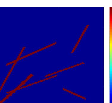
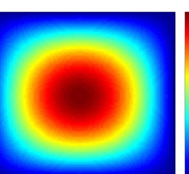
Figure 2: The heterogeneous permeability field: $\kappa$ (left) and source term $f=2\pi^{2}\sin(\pi x_{1})\sin(\pi x_{2})$ (right).

The fractional derivative order is chosen to be $\alpha:=0.9$. For the brevity of the paper, we will only present numerical solutions at the final time $T$. The fine-grid solution, CEM solution, CEM solution with more basis functions and SCEM solution at the final time $T$ are plotted in Figure 3.

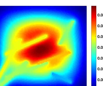
Figure 3: fine-grid solution $u_{h}^{2500}$ (top left), CEM solution $U_{cem}^{500}$ (top right), CEM solution with additional basis functions implicitly $\tilde{U}^{500}$ (bottom left), SCEM solution with additional basis functions explicitly $u_{scem}^{500}$ (bottom right).

The convergence history of three numerical solutions in relative $L^{2}(\Omega)$-norm and relative $H^{1}_{\kappa}(\Omega)$-norm are presented in Figure 4. From Figure 4, one can see that when using the same number of basis functions, SCEM solutions are better approximations than CEM solutions to the reference solutions. Moreover, numerical solutions $u_{scem}$ and $\tilde{U}$ have about the similar accuracy. However, it is computationally cheaper to solve for $u_{scem}$ than $\tilde{U}$.

Furthermore, we test the experiment with different value of fractional derivative order $\alpha$. It turns out that when we choose $\alpha=0.5,0.4,0.3$, the SCEM solutions become unstable. This observation is confirmed by the stability condition that $\left\|v\right\|\geq\alpha_{0}(1-\gamma^{2})^{-1}\left\|v\right\|_{a}^{2}$ hold true for any $v\in V_{H,2}$.

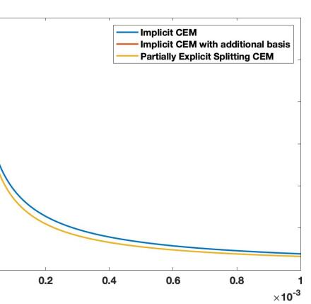
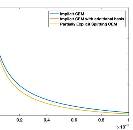
Figure 4: Relative $L^{2}(\Omega)$ error (left) and Relative $H^{1}_{\kappa}(\Omega)$ error (right).

5.2 Numerical Experiment 2: discontinuous source term

In the second experiment, we choose a heterogeneous permeability coefficient $\kappa$, which has two distinct value: 1 and $10^{5}$. The source term $f$ is chosen to be a discontinuous function. They are plotted in Figure 5 for an illustration.

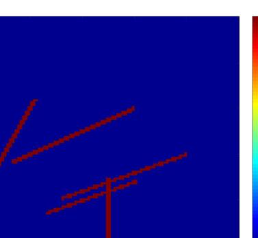
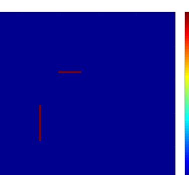
Figure 5: The heterogeneous permeability field: $\kappa$ (left) and source term $f$ (right).

We first choose The fractional derivative order $\alpha:=0.9$. The fine-grid solution, CEM solution, CEM solution with more basis functions and SCEM solution at the final time $T$ are plotted in Figure 6.

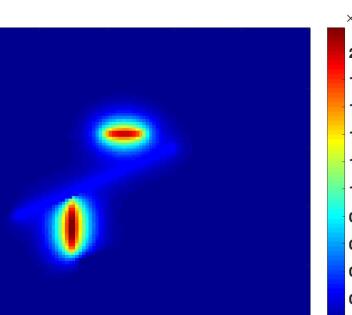
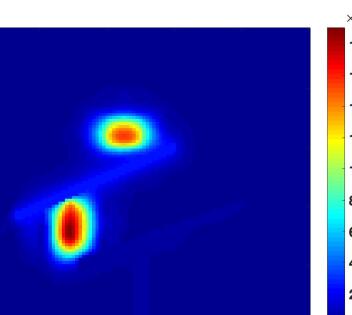
Figure 6: fine-grid solution $u_{h}^{2500}$ (top left), CEM solution $U_{cem}^{500}$ (top right), CEM solution with additional basis functions implicitly $\tilde{U}^{500}$ (bottom left), SCEM solution with additional basis functions explicitly $u_{scem}^{500}$ (bottom right).

The convergence history of three numerical solutions in relative $L^{2}(\Omega)$-norm and relative $H^{1}_{\kappa}(\Omega)$-norm are presented in Figure 7. In this experiment, we have similar observations as Experiment 1. That is, $u_{scem}$ has about similar accuracy as $\tilde{U}$ and it is cheaper to compute $u_{scem}$ than $\tilde{U}$.

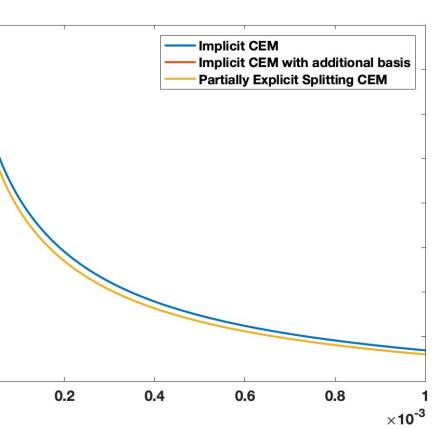
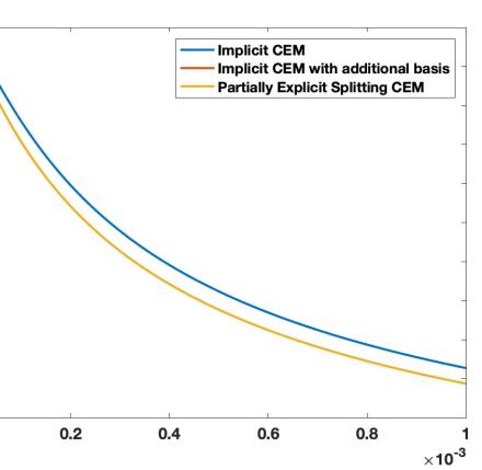
Figure 7: L2 error (left) and Energy error (right).

6 Conclusions

In this paper, we present a framework for partial explicit discretization for time fractional PDEs. The work is motivated by many applications of multiscale time fractional PDEs. Explicit time discretization for time fractional PDEs requires very small time steps due to size of the fine grid, the contrast, and additional power that is associated with the fractional power of the time derivative. Our approach solves time fractional PDEs on a coarse grid by constructing appropriate coarse spaces. We show that the proposed method is stable and one can choose the time step that does not depend on the contrast and only depends on the coarse mesh size. We note that our approach does not remove the constraint related to the power of the time fractional PDE. Via the construction of appropriate spaces and careful stability analysis, we can show that the time step can be chosen not to depend on the contrast and scale as the coarse mesh size. We present numerical results by considering time fractional diffusion in highly heterogeneous media. We show that the proposed partial explicit approach provides similar results compared to the fully implicit method, where all degrees of freedom are treated implicitly.

References

- [1] K. Aleksandrovich, H. M. Srivastava, and J. J. Trujillo. Theory and applications of fractional differential equations, volume 204. elsevier, 2006.
- [2] A. A. Alikhanov. A new difference scheme for the time fractional diffusion equation. Journal of Computational Physics, 280:424–438, 2015.
- [3] A. A. Alikhanov and C. Huang. A high-order l2 type difference scheme for the time-fractional diffusion equation. arXiv preprint arXiv:2102.08813, 2021.
- [4] D. L. Brown, Y. Efendiev, and V. H. Hoang. An efficient hierarchical multiscale finite element method for stokes equations in slowly varying media. Multiscale Modeling & Simulation, 11(1):30–58, 2013.
- [5] D. L. Brown, J. Gedicke, and D. Peterseim. Numerical homogenization of heterogeneous fractional laplacians. Multiscale Modeling & Simulation, 16(3):1305–1332, 2018.
- [6] K. Chukbar. Stochastic transport and fractional derivatives. Technical report, Rossijskij Nauchnyj Tsentr’Kurchatovskij Inst.’, 1994.
- [7] E. T. Chung, Y. Efendiev, and T. Hou. Adaptive multiscale model reduction with generalized multiscale finite element methods. Journal of Computational Physics, 320:69–95, 2016.
- [8] E. T. Chung, Y. Efendiev, and C. Lee. Mixed generalized multiscale finite element methods and applications. SIAM Multiscale Model. Simul., 13:338–366, 2014.
- [9] E. T. Chung, Y. Efendiev, and W. T. Leung. Generalized multiscale finite element methods for wave propagation in heterogeneous media. Multiscale Modeling & Simulation, 12(4):1691–1721, 2014.
- [10] E. T. Chung, Y. Efendiev, and W. T. Leung. Constraint energy minimizing generalized multiscale finite element method. Computer Methods in Applied Mechanics and Engineering, 339:298–319, 2018.
- [11] E. T. Chung, Y. Efendiev, and W. T. Leung. Constraint energy minimizing generalized multiscale finite element method in the mixed formulation. Computational Geosciences, 22(3):677–693, 2018.
- [12] E. T. Chung, Y. Efendiev, and W. T. Leung. Fast online generalized multiscale finite element method using constraint energy minimization. Journal of Computational Physics, 355:450–463, 2018.
- [13] E. T. Chung, Y. Efendiev, W. T. Leung, and P. N. Vabishchevich. Contrast-independent partially explicit time discretizations for multiscale flow problems, 2021.
- [14] E. T. Chung, Y. Efendiev, W. T. Leung, M. Vasilyeva, and Y. Wang. Non-local multi-continua upscaling for flows in heterogeneous fractured media. Journal of Computational Physics, 372:22–34, 2018.
- [15] W. E and B. Engquist. Heterogeneous multiscale methods. Comm. Math. Sci., 1(1):87–132, 2003.
- [16] Y. Efendiev, J. Galvis, and T. Hou. Generalized multiscale finite element methods (GMsFEM). Journal of Computational Physics, 251:116–135, 2013.
- [17] Y. Efendiev and T. Hou. Multiscale Finite Element Methods: Theory and Applications, volume 4 of Surveys and Tutorials in the Applied Mathematical Sciences. Springer, New York, 2009.
- [18] Y. Efendiev, S.-M. Pun, and P. N. Vabishchevich. Temporal splitting algorithms for non-stationary multiscale problems. Journal of Computational Physics, page 110375, 2021.
- [19] Y. Efendiev and P. N. Vabishchevich. Splitting methods for solution decomposition in nonstationary problems. Applied Mathematics and Computation, 397:125785, 2021.
- [20] G.-h. Gao, Z.-z. Sun, and H.-w. Zhang. A new fractional numerical differentiation formula to approximate the caputo fractional derivative and its applications. Journal of Computational Physics, 259:33–50, 2014.
- [21] M. Giona, S. Cerbelli, and H. E. Roman. Fractional diffusion equation and relaxation in complex viscoelastic materials. Physica A: Statistical Mechanics and its Applications, 191(1-4):449–453, 1992.
- [22] P. Henning, A. Målqvist, and D. Peterseim. A localized orthogonal decomposition method for semi-linear elliptic problems. ESAIM: Mathematical Modelling and Numerical Analysis, 48(5):1331–1349, 2014.
- [23] R. Hilfer. Applications of fractional calculus in physics. World scientific, 2000.
- [24] T. Hou and X. Wu. A multiscale finite element method for elliptic problems in composite materials and porous media. J. Comput. Phys., 134:169–189, 1997.
- [25] T. Y. Hou, D. Huang, K. C. Lam, and P. Zhang. An adaptive fast solver for a general class of positive definite matrices via energy decomposition. Multiscale Modeling & Simulation, 16(2):615–678, 2018.
- [26] T. Y. Hou, Q. Li, and P. Zhang. Exploring the locally low dimensional structure in solving random elliptic pdes. Multiscale Modeling & Simulation, 15(2):661–695, 2017.
- [27] T. Y. Hou, D. Ma, and Z. Zhang. A model reduction method for multiscale elliptic pdes with random coefficients using an optimization approach. Multiscale Modeling & Simulation, 17(2):826–853, 2019.
- [28] J. Hu and G. Li. Homogenization of time-fractional diffusion equations with periodic coefficients. Journal of Computational Physics, 408:109231, 2020.
- [29] P. Jenny, S. Lee, and H. Tchelepi. Multi-scale finite volume method for elliptic problems in subsurface flow simulation. J. Comput. Phys., 187:47–67, 2003.
- [30] A. A. Kilbas, H. M. Srivastava, and J. J. Trujillo. Theory and Applications of Fractional Differential Equations, volume 204 of North-Holland Mathematics Studies. Elsevier Science B.V., Amsterdam, 2006.
- [31] S. C. Kou. Stochastic modeling in nanoscale biophysics: subdiffusion within proteins. The Annals of Applied Statistics, 2(2):501–535, 2008.
- [32] C. Le Bris, F. Legoll, and A. Lozinski. An MsFEM type approach for perforated domains. Multiscale Modeling & Simulation, 12(3):1046–1077, 2014.
- [33] Y. Lin and C. Xu. Finite difference/spectral approximations for the time-fractional diffusion equation. J. Comput. Phys., 225(2):1533–1552, 2007.
- [34] G. I. Marchuk. Splitting and alternating direction methods. Handbook of numerical analysis, 1:197–462, 1990.
- [35] R. Nigmatullin. The realization of the generalized transfer equation in a medium with fractal geometry. Physica Status Solidi (b), 133(1):425–430, 1986.
- [36] K. Oldham and J. Spanier. The fractional calculus theory and applications of differentiation and integration to arbitrary order. Elsevier, 1974.
- [37] H. Owhadi and L. Zhang. Metric-based upscaling. Comm. Pure. Appl. Math., 60:675–723, 2007.
- [38] I. Podlubny. Fractional differential equations: an introduction to fractional derivatives, fractional differential equations, to methods of their solution and some of their applications. Elsevier, 1998.
- [39] I. Podlubny. Fractional Differential Equations, volume 198 of Mathematics in Science and Engineering. Academic Press, Inc., San Diego, CA, 1999. An introduction to fractional derivatives, fractional differential equations, to methods of their solution and some of their applications.
- [40] A. Roberts and I. Kevrekidis. General tooth boundary conditions for equation free modeling. SIAM J. Sci. Comput., 29(4):1495–1510, 2007.
- [41] G. Samaey, I. Kevrekidis, and D. Roose. Patch dynamics with buffers for homogenization problems. J. Comput. Phys., 213(1):264–287, 2006.
- [42] H. Scher and E. W. Montroll. Anomalous transit-time dispersion in amorphous solids. Physical Review B, 12(6):2455, 1975.
- [43] Z.-Z. Sun, C.-C. Ji, and R. Du. A new analytical technique of the l-type difference schemes for time fractional mixed sub-diffusion and diffusion-wave equations. Applied Mathematics Letters, 102:106115, 2020.
- [44] P. N. Vabishchevich. Additive Operator-Difference Schemes: Splitting Schemes. Walter de Gruyter GmbH, Berlin, Boston, 2013.
- [45] Y.-n. Zhang, Z.-z. Sun, and H.-l. Liao. Finite difference methods for the time fractional diffusion equation on non-uniform meshes. Journal of Computational Physics, 265:195–210, 2014.