Dissimilar collective decay and directional emission from two quantum emitters

Abstract

We study a system of two distant quantum emitters coupled via a one-dimensional waveguide where the electromagnetic field has a direction-dependent velocity. As a consequence, the onset of collective emission is non-simultaneous and, for appropriate parameters, while one of the emitters exhibits superradiance the other can be subradiant. Interference effects enable the system to radiate in a preferential direction depending on the atomic state and the field propagation phases. We characterize such directional emission as a function of various parameters, delineating the conditions for optimal directionality.

1 Introduction

Engineering atom-photon interactions by manipulating electromagnetic (EM) fields is a significant aspect of design and implementation of quantum technologies [1, 2, 3]. For instance, reducing the mode volume of the EM field enhances the light-matter coupling [4] and controlling the field polarization allows for chiral interactions between quantum emitters with polarization-dependent transitions [5]. Current platforms allow one to change yet another property of the EM field: its propagation velocity [6, 7, 8]. In particular, one can envision the possibility of having an EM field with unequal velocities when propagating to the left or to the right, here referred to as anisotachy . Such feature is, as yet, an unexplored aspect of quantum optical systems, which could be implemented with state-of-the art non-reciprocal components [9, 10]. Since the propagation velocity is an essential ingredient in connecting the distant parts of a larger system, the effects of anisotachy are expected to appear when measuring properties that depend on the interaction between delocalized subsystems, such as quantum correlations.

Quantum correlations among emitters can collectively enhance or inhibit light absorption and emission [11]. For example, a collection of emitters can radiate faster or slower than individual ones depending on their correlations, phenomena known as super- and sub-radiance respectively . These effects have been extensively studied both theoretically [12, 11, 13, 14, 15, 16] and experimentally across various platforms [17, 18, 19, 20, 21, 22, 23, 24, 25, 26, 27, 28, 29]. Recent works have proposed, and implemented [30], collective effects for controlling the direction of emission using the non-local correlations between two emitters, with potential applications in quantum information processing and quantum error correction [31, 32, 33, 34]

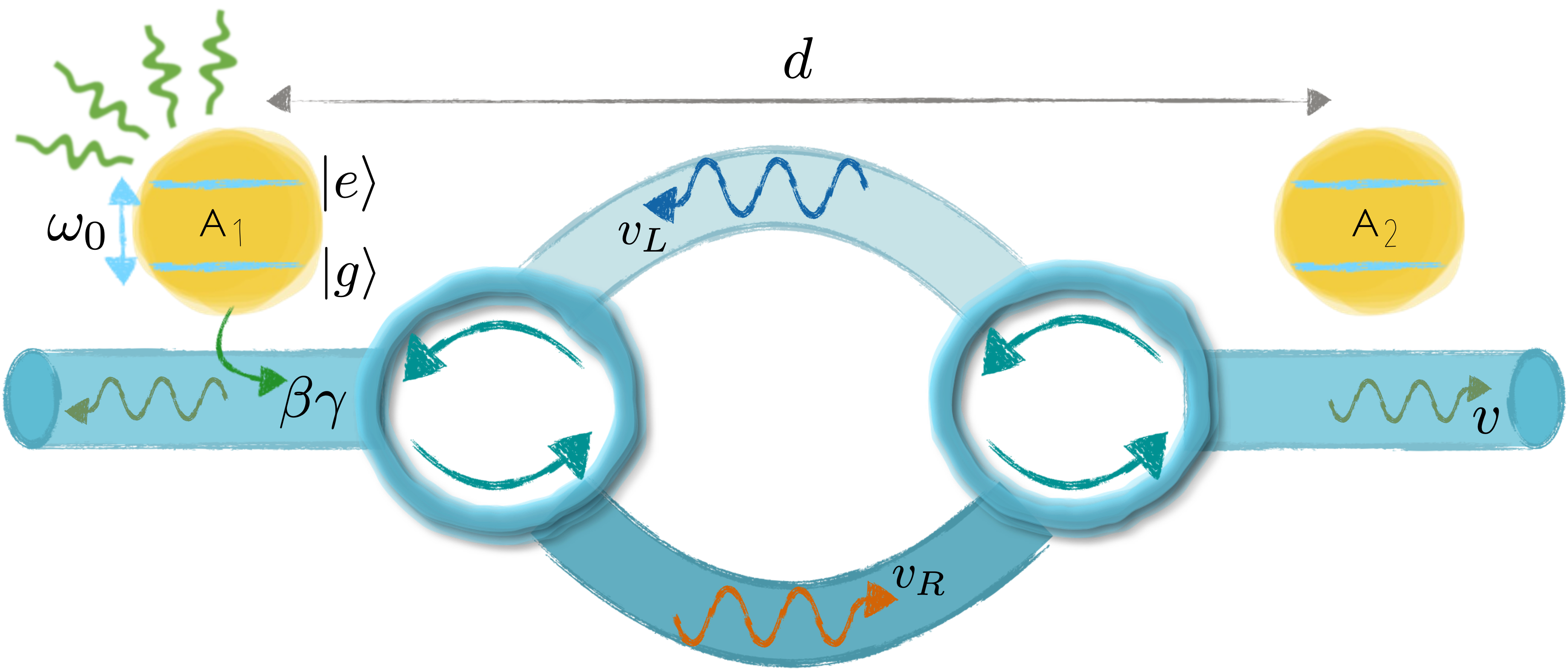
Figure 1: Schematic representation of two two-level atoms coupled to a waveguide with an interatomic separation $d$. The waveguide connects to two circulators that are coupled to two separate waveguides with different field velocities, such that the left (right) propagating modes have a velocity $v_{\rm{L}}$ $(v_{\rm{R}})$. The atoms have a resonance frequency $\omega_{0}$ and a decay rate $\gamma$, and couple to the waveguide with a coupling efficiency $\beta$. The velocity of the field in the waveguide outside of the circulator region is $v$.

In this work we propose a system comprising of two distant quantum emitters or atoms coupled to a one-dimensional waveguide with an effective direction-dependent field velocity, or anisotachy. As we will show, a direction-dependent time delay can allow two correlated emitters to exhibit disparate collective effects such that while one atom decays superradiantly, the other exhibits subradiance. In such a system, interference effects in the radiated field lead to a directional emission. We characterize such directional emission as a function of initial states of the emitters, field propagation phases, and the waveguide coupling efficiency. Our results demonstrate that collective directional emission is a rather prevalent quantum optical phenomenon that needs further exploration, to understand its advantages, limitations and dependence on a broader set of parameters.

We first present a theoretical model of the system, describing the disparate cooperative decay dynamics of the emitters and the radiated field intensity in the presence of anisotachy. We then characterize the optimum conditions for directional emission. Finally we discuss the experimental feasibility and give a brief outlook of the phenomena.

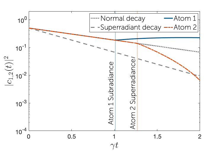
(a)

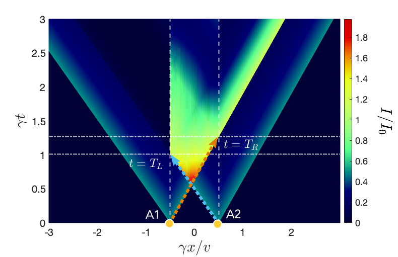
(b)

Figure 2: Atomic excitation probability and intensity dynamics for emitters prepared initially in the symmetric state $\left|\Phi_{0}\right\rangle=\frac{1}{\sqrt{2}}\left(\left|eg\right\rangle+\left|ge\right\rangle\right)$, with $\phi_{\rm{L}}=\pi$ and $\phi_{\rm{R}}=2\pi$. (a) The blue solid and red dash-dotted curves represent the populations of atoms A1 and A2 respectively, with the dotted vertical lines indicating the onset of collective emission. The gray dotted and dashed curves represent standard individual and superradiant decay, respectively. (b) Intensity of the radiated field as a function of spacetime. The vertical dashed lines indicate the position of the two atoms while the horizontal dash-dotted lines represent the times $t=T_{L}$ and $t=T_{R}$. Here we have chosen the dimensionless atomic separation $\gamma d/v\approx 1$, propagation velocities $v_{\rm{L}}/v\approx 0.988$ and $v_{\rm{R}}/v\approx 0.788$, $\omega_{0}/\gamma\approx 500$ and coupling efficiency $\beta\approx 1$.

2 Model

Let us consider two two-level quantum emitters coupled to the EM field modes of a waveguide. Using field circulators, the field modes propagate through different waveguides with unequal index of refraction, as shown in Fig. 1, leading to an effective anisotachy.

The Hamiltonian for the system is given as $H=H_{E}+H_{F}+H_{EF}$, where $H_{E}=\sum_{m=1,2}\hbar\omega_{0}\hat{\sigma}_{m}^{+}\hat{\sigma}_{m}^{-}$ is the Hamiltonian for the emitters, with $\left\{\hat{\sigma}_{m}^{+},\hat{\sigma}_{m}^{-}\right\}$ as the raising and lowering operators for the $m^{\mathrm{th}}$ atom. $H_{F}=\int_{0}^{\infty}\mathrm{d}\omega\,\hbar\omega\left[\hat{a}_{\mathrm{R}}^{\dagger}\left(\omega\right)\hat{a}_{\mathrm{R}}\left(\omega\right)+\hat{a}_{\mathrm{L}}^{\dagger}\left(\omega\right)\hat{a}_{\mathrm{L}}\left(\omega\right)\right],$ corresponds to the Hamiltonian for the guided modes of the waveguide, with $\hat{a}_{\rm{L(R)}}^{(\dagger)}$ as the bosonic operators for the left (right) propagating modes. The interaction Hamiltonian in the interaction picture with respect to the free Hamiltonians $H_{E}+H_{F}$ is [35, 36]

$$\tilde{H}_{EF}= \sum_{m=1,2}\int_{0}^{\infty}\mathrm{d}\omega\,\hbar g\left(\omega\right)\left[\hat{\sigma}_{m}^{+}\left\{\hat{a}_{\rm{R}}\left(\omega\right)e^{ik_{\rm{R}}x_{m}}\right.\right.$$

$$\left.\left.+\hat{a}_{\rm{L}}\left(\omega\right)e^{-ik_{\rm{L}}x_{m}}\right\}e^{-i\left(\omega-\omega_{0}\right)t}+\rm{H.C.}\right],$$ (1)

where $x_{1}=-x_{2}=-d/2$ denotes the position of the emitters, $g(\omega)$ represents the atom-field coupling strength and $k_{L,R}\equiv\omega/v_{L,R}$ corresponds to the asymmetric left and right wavenumbers. Considering the initial state of the system with the emitters being in the single excitation sub-space and the field in vacuum,

$$\left|\Psi(t)\right\rangle=\left[\sum_{m=1,2}c_{m}(t)\hat{\sigma}_{m}^{+}+\int_{0}^{\infty}\mathrm{d}\omega\,\left\{c_{\rm{R}}(\omega,t)\hat{a}_{\rm{R}}^{\dagger}\left(\omega\right)\right.\right.$$

$$\left.\left.+c_{\rm{L}}(\omega,t)\hat{a}_{\rm{L}}^{\dagger}\left(\omega\right)\right\}\right]\left|gg\right\rangle\otimes\left|\left\{0\right\}\right\rangle$$ , (2)

one can derive the equations of motion for the atomic coefficients, $c_{1}$ and $c_{2}$, using a Wigner-Weisskopf approach as (see Appendix A for details)

$$\dot{c}_{1(2)}\left(t\right)=- \frac{\gamma}{2}\left[c_{1(2)}\left(t\right)\right.$$

$$\left.+\beta c_{2(1)}\left(t-T_{\rm{L(R)}}\right)\Theta\left(t-T_{\rm{L(R)}}\right)e^{i\omega_{0}T_{\rm{L(R)}}}\right].$$ (3)

Here $\gamma$ is the total spontaneous emission rate, $\beta\gamma=4\pi|g(\omega_{0})|^{2}$ is the decay rate into the guided modes, and $T_{\rm{R}(\rm{L})}=d/v_{\rm{R}(\rm{L})}$ is the propagation time of the field traveling right (left) from one emitter to the other.

3 Dynamics

Let us consider the initial state of the emitters to be $\left|\Psi_{0}\right\rangle\equiv c_{1}(0)\left|eg\right\rangle+c_{2}(0)\left|ge\right\rangle$. The equations of motion (Eq. (3)) can be solved to obtain (see Appendix B):

$$c_{1(2)}(t)= \sum_{n=0}^{\infty}\underbrace{\boxed{c_{1(2)}(0)e^{i2n\phi}}\frac{\left(\beta\gamma/2\right)^{2n}}{(2n)!}\left(t-2nT\right)^{2n}e^{-\gamma\left(t-2nT\right)/2}\Theta\left(t-2nT\right)}_{\text{Even number of trips between atoms}}$$

$$-\sum_{n=0}^{\infty}\underbrace{\boxed{c_{2(1)}(0)e^{i2n\phi+i\phi_{L(R)}}}\frac{\left(\beta\gamma/2\right)^{2n+1}}{(2n+1)!}\left(t-2nT-T_{L(R)}\right)^{2n+1}e^{-\gamma\left(t-2nT-T_{L(R)}\right)/2}\Theta\left(t-2nT-T_{L(R)}\right)}_{\text{Odd number of trips between atoms}},$$ (4)

where $\phi_{\rm{R}(\rm{L})}=\omega_{0}T_{\rm{R}(\rm{L})}$ is the phase acquired by the resonant field upon propagation between the emitters, and $T=(T_{\rm{R}}+T_{\rm{L}})/2$ and $\phi=(\phi_{\rm{R}}+\phi_{\rm{L}})/2$ are the average propagation time and phase respectively . The first term in the equation above represents the modification of atomic decay after $n$ round trips of the field between the emitters. The second term represents an odd-number of trips $(2n+1)$ from one emitter to the other. The directional propagation phase ($\phi_{\rm{R}(\rm{L})}$), together with the phase from the atomic coefficients ($c_{2(1)}$), determines the constructive or destructive nature of interference between the two terms, as indicated by the boxed terms.

Fig. 2 (a) shows the decay of the atomic excitation coefficients as a function of time. Destructive (constructive) interference in the left (right) propagating modes leads to a subradiant atom A1 and a superradiant atom A2, after the field from one atom reaches the other. One can thus interpret collective decay as a mutually stimulated emission process, as is evident from the series expansion in Eq. (4). For a negligible separation between emitters $(T\rightarrow 0)$, the series converges to yield the standard superradiant exponential decay. In the presence of delay, the resulting dynamics is more precisely described as a cascade of stimulated emission processes [42]. For instance, the field from one emitter can stimulate emission of the other, leading to a non-exponential decay that is faster than superradiance [37, 40, 41, 43], or completely suppress its emission, leading to bound states in the continuum (BIC) [38, 44]. More generally, this effect can accelerate the decay of one atom while slowing the decay of the other, as shown in Fig. 2 (a). This demonstrates that the phenomena of super- and subradiance are not a characteristic of the system as a whole, rather an effective description of local atom-photon interference effects.

$\phi_{L}$	$\phi_{R}$	$\phi_{A1}-\phi_{A2}$	Atom 1	Atom 2
$2n\pi$	$(2m+1)\pi$	$0$	Superradiant	Subradiant	Anisotachy
		$\pi$	Subradiant	Superradiant	required
$(2n+1)\pi$	$2m\pi$	$0$	Subradiant	Superradiant	Anisotachy
		$\pi$	Superradiant	Subradiant	required
$(n+\frac{1}{2})\pi$	$(m+\frac{1}{2})\pi$	$\frac{\pi}{2}$	Subradiant	Superradiant	No anisotachy
		-$\frac{\pi}{2}$	Superradiant	Subradiant	required

Table 1: Some representative examples of dissimilar collective decay for different atomic and field propagation phases.

One can note a few salient features of the collective atomic dynamics from the above equation:

• Each term in the series expansion can be interpreted as multiple partial reflections of a field wave packet bouncing between the atoms at signaling times $t=2nd/v$ and $2nd/v+d/v_{L(R)}$, as denoted by the theta-functions ($\Theta\left(t-2nd/v\right)$ and $\Theta\left(t-2nd/v-d/v_{L(R)}\right)$). This offers the intuition that the collective decay dynamics arises from a cascade of stimulated emission processes as the field emitted by the each of the atoms propagates back and forth between them.

• The interference phase for all partial reflections is determined by the phase factors $c_{1(2)}(0)e^{i2n\phi}$ and $c_{2(1)}(0)e^{i2n\phi+i\phi_{L(R)}}$, which is a combination of the atomic and field propagation phases. Each successive term comes with an additional factor of the atom-waveguide coupling strength $\beta\gamma/2$.

• The propagation phases $\phi_{L(R)}$ can be different in the presence of anisotachy, which can make the contribution from the second term to the collective dynamics different for the two atoms, thus leading to dissimilar collective behavior. We summarize a few example cases of such behavior in Table 1.

The EM field intensity emitted by the system, as a function of position $x$ and time $t$, can be evaluated as $I\left(x,t\right)=\frac{\epsilon_{0}c}{2}\left\langle\Psi\left(t\right)|\hat{E}^{\dagger}\left(x,t\right)\hat{E}\left(x,t\right)|\Psi\left(t\right)\right\rangle$ (see Appendix C):

$$\frac{I(x,t)}{I_{0}}=\left|\left[\underbrace{C_{1}\left(t,\left(x+d/2\right)/v_{\rm{L}}\right)e^{-i\omega_{0}\left(x+d/2\right)/v_{\rm{L}}}}_{\text{Atom 1 left light cone}}+\underbrace{C_{2}\left(t,\left(x-d/2\right)/v_{\rm{L}}\right)e^{-i\omega_{0}\left(x-d/2\right)/v_{\rm{L}}}}_{\text{Atom 2 left light cone}}\right.\right.$$

$$\left.\left.+\underbrace{C_{1}\left(t,-\left(x+d/2\right)/v_{\rm{R}}\right)e^{i\omega_{0}\left(x+d/2\right)/v_{\rm{R}}}}_{\text{Atom 1 right light cone}}+\underbrace{C_{2}\left(t,-\left(x-d/2\right)/v_{\rm{R}}\right)e^{i\omega_{0}\left(x-d/2\right)/v_{\rm{R}}}}_{\text{Atom 2 right light cone}}\right]\right|^{2},$$ (5)

where we have redefined the atomic excitation coefficients $C_{i}\left(t,\tau\right)=c_{i}\left(t+\tau\right)\zeta\left(t,\tau\right)$ to explicitly include the causal dynamics in the notation, with $\zeta(t_{1},t_{2})\equiv\Theta(t_{1}+t_{2})-\Theta(t_{2})$. The first (last) two terms above correspond to the left-(right-) going light cones emitted from the atoms A1 and A2. Fig. 2 (b) shows the radiated intensity with the emitted fields destructively (constructively) interfering to the left (right) leading to almost perfect directional emission.

4 Directional emission

We characterize the probability of emitting the photon into the right (left) propagating mode by $P_{\rm{R(L)}}(\Psi_{0})=\lim_{t\rightarrow\infty}\int_{0}^{\infty}\mathrm{d}\omega\left|c_{\rm{R(L)}}\left(\omega,t\right)\right|^{2}$, with $P_{\rm{R(L)}}(\Psi_{0})$ as an explicit function of the initial state $\left|\Psi_{0}\right\rangle$ (see Appendix D). We focus here on the limit of small atomic separation $\gamma T\ll 1$ such that retardation effects are negligible. For convenience we write the initial condition as $c_{1}(0)=\cos\theta e^{i\phi_{\rm{A1}}}$ and $c_{2}(0)=\sin\theta e^{i\phi_{\rm{A2}}}$. The probability of emitting in a particular direction is a function of four parameters: the coupling efficiency $\beta$, the average propagation phase $\phi$; the initial atomic populations parametrized by $\theta$; and the difference between the relative atomic and propagation phases $\Delta\phi=(\phi_{\rm{A1}}-\phi_{\rm{A2}})+(\phi_{\rm{R}}-\phi_{\rm{L}})/2$. For a given experimental realization, the parameters $\beta$ and $\phi$ would be fixed, and the variable atomic parameters $\theta$ and $\Delta\phi$ would determine the directionality of emission.

The directional emission of the system can be characterized by $\chi=\left(P_{\rm{R}}-P_{\rm{L}}\right)/\left(P_{\rm{R}}+P_{\rm{L}}\right)$, which can be calculated explicitly as (see Appendix D)

$$\chi(\Psi_{0})=-\frac{\beta\sin\phi}{P_{\rm{tot}}}\left(\frac{\sin\Delta\phi\sin 2\theta+\beta\cos 2\theta\sin\phi}{1+\left(\beta\sin\phi\right)^{2}}\right),$$ (6)

where $P_{\mathrm{tot}}=P_{\mathrm{R}}+P_{\mathrm{L}}$ is the total probability of emitting into the waveguide:

$$P_{\rm{tot}}(\Psi_{0}) =$$

$$\beta\left[\frac{1-\beta\cos^{2}\phi-\left(\beta-1\right)\cos\Delta\phi\cos\phi\sin 2\theta}{1-\left(\beta\cos\phi\right)^{2}}\right].$$ (7)

We note from the above that $P_{\mathrm{tot}}=\beta$ only for $\phi=\left(n+\frac{1}{2}\right)\pi$, more generally, the interference in the field enhances or inhibits the effective coupling efficiency between the emitters and the waveguide. Eq. (6) shows that the emission is typically directional for most values of $\Delta\phi$ and $\phi\neq N\pi$, $N\in\mathbb{N}$. This indicates a prevalence of directional emission in quantum optical systems.

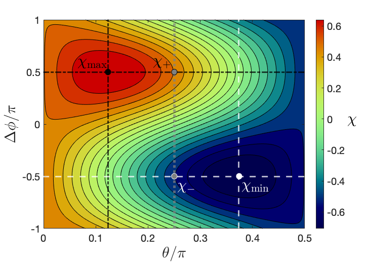
(a)

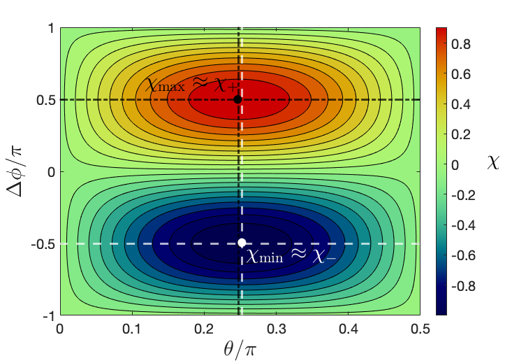
(b)

Figure 3: Directionality parameter $\chi$ as a function of the initial atomic state parameters, for waveguide coupling efficiencies of (a) $\beta=1$ (b) $\beta=0.01$. The propagation phase is fixed to be $\phi=\pi/2$ and the atomic separation is considered to be in the non-retarded regime $(\gamma T\ll 1)$. (a) For $\beta=1$, the maximum directionality is obtained for $\theta=\pi/8$ and $\Delta\phi=\pm\pi/2$ with a maximum and minimum $\chi$ values of $\chi_{\mathrm{max}}=-\chi_{\mathrm{min}}=1/\sqrt{2}$. The gray points indicate directional emission obtained for initial states $\left|eg\right\rangle\pm i\left|ge\right\rangle$ with a $\chi_{\pm}=\pm 1/2$ [32]. (b) For $\beta=0.01$ the directional parameter can be as large as $\chi_{\mathrm{max}}=-\chi_{\mathrm{min}}\approx 0.999$.

Fig. 3 shows the directionality of photon emission $\chi$ as a function of the parameters of the initial atomic state for the optimum directionality condition $\phi=\left(n+\frac{1}{2}\right)\pi$, for two particular waveguide coupling efficiencies $(\beta=1$ and $0.01)$. Considering two orthogonal entangled atomic states $\left|\Psi_{a(b)}\right\rangle=\frac{1}{\sqrt{2}}\left(\left|eg\right\rangle+e^{i\varphi_{a(b)}}\left|ge\right\rangle\right)$ with $\varphi_{a}-\varphi_{b}=\pi$, we obtain a directional parameter value $\chi_{a(b)}=\sin\left(\phi_{R}-\phi_{L}-\varphi_{a(b)}\right)/\left(1+\beta^{2}\right)$. It can be thus seen that appropriately manipulating the relative field propagation phase $(\phi_{R}-\phi_{L})$ can allow one to distinguish any two orthogonal entangled states based on the direction of emission, as illustrated by the points $\chi_{+}$ and $\chi_{-}$ on Fig. 3.

We note that the directional emission from an entangled state benefits from $\beta<1$ as can be seen from comparing Fig. 3 (a) and (b). This can be understood from the series expansions in Eqs. (4), where the terms with odd powers of $\beta$ contribute to the directionality, while terms of order $\beta^{2}$ are detrimental. This contrasts with the standard case of neglecting field propagation, where $\beta<1$ does not change the qualitative behaviour of guided emission. In the limit $\beta\ll 1$

$$\chi(\Psi_{0})\approx-\mathcal{C}\sin\phi\sin\Delta\phi,$$ (8)

where $\mathcal{C}=\sin 2\theta$ is the concurrence that characterizes the entanglement of a pure state $\left|\Psi_{0}\right\rangle$. Thus, for small waveguide coupling efficiencies, the directionality $\chi$ could be a direct measure of the entanglement of the emitters. This also indicates that directional emission can be observed even in experiments with low coupling efficiency between emitters and waveguides.

We discuss the various parameter dependencies of the directionality below:

• Dependence on average propagation phase $\left(\phi=\frac{\phi_{R}+\phi_{L}}{2}\right)$: Directionality comes from having constructive interference in one direction and destructive interference in the other direction. Considering the phases of field propagation $\phi_{R}=2n\pi$ and $\phi_{L}=\left(2m+1\right)\pi$, gives $\phi=\left(n+\frac{1}{2}\right)\pi$. We see that this maximizes the overall prefactor $\sin\phi$ and thus the directionality.

• Dependence on the relative atomic and field phases $\left(\Delta\phi\right)$: The interference effects between the atomic dipoles and the field are represented by the $\sin\Delta\phi$ term, which maximizes directionality for $\sin\Delta\phi\rightarrow 1$. This can be clearly seen from both Fig. 3 (a) and (b).

• Dependence on waveguide coupling efficiency $(\beta)$ and initial atomic excitation amplitudes ($\theta$): In the case of $\beta\rightarrow 0$, there is nearly zero probability of multiple reflections, absorptions, and reemissions of the field in the waveguide, such that the field from one atom perfectly interferes (constructive or destructively) with the field from the other atom. For $\beta\rightarrow 1$, the optimum directionality occurs when one atom radiates most of the field, while the second provides just enough field required for constructive interference (as seen from Fig.3 (a)). This case corresponds to the optimum value $\theta=\pi/8$.

Directionality can aid in sensing either the relative atomic phases or field propagation phases $\varphi$ , all other experimental parameters being fixed. In order to quantify this advantage we define $\mathcal{F}_{D}\left(\varphi\right)\equiv\sum_{i=L,R,\mathrm{out}}P_{i}\left(\partial\log\left[P_{i}\right]/\partial\varphi\right)^{2}$ as the Fisher information that considers directionality. Here $P_{i}$ is the probability of emission into the decay channel $i$, spanning over modes propagating to the left $(P_{\rm{L}})$, right $(P_{\rm{R}})$, and out of the waveguide $(P_{\rm{out}}=1-(P_{\rm{R}}+P_{\rm{L}}))$. To compare with the case where one ignores directionality, we define the non-directional Fisher information $\mathcal{F}_{\rm{ND}}\left(\varphi\right)\equiv\sum_{i=\mathrm{tot},\mathrm{out}}P_{i}\left(\partial\log\left[P_{i}\right]/\partial\varphi\right)^{2}$, that considers only the total decay into and outside the waveguide with probabilities $P_{\rm{tot}}$ and $P_{\rm{out}}$, respectively. It can be shown that $\mathcal{F}_{D}\left(\varphi\right)\geq\mathcal{F}_{ND}\left(\varphi\right)$ (see Appendix . D), meaning that distinguishing the direction of propagation of the emitted photon helps to better estimate the general phase $\varphi$.

5 Implementation in a circuit QED system

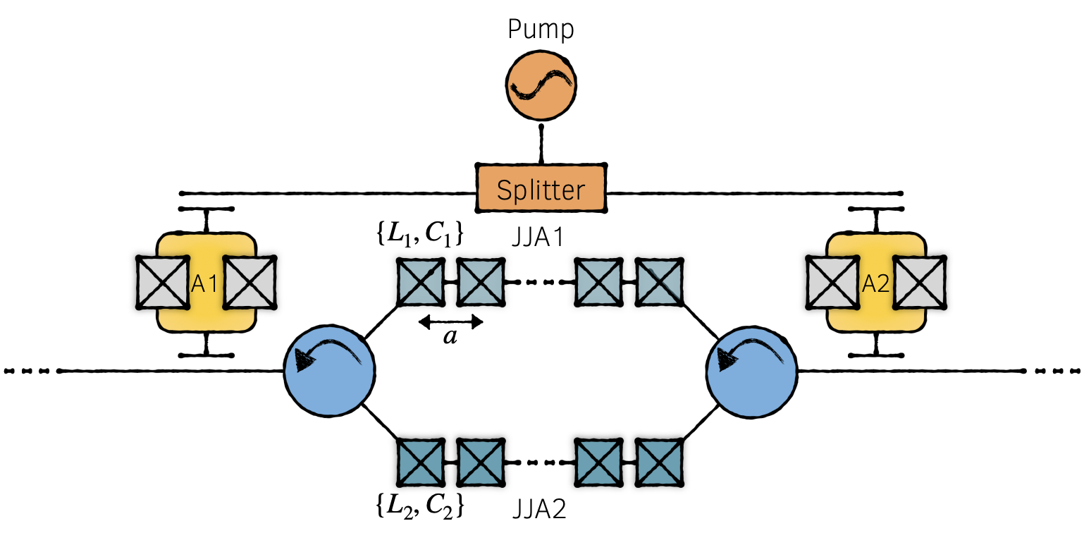
Figure 4: Schematic representation of a circuit QED implementation of the model. Two transmons (A1 and A2) coupled via circulators and Josephson junction (JJ) arrays (JJA1 and JJA2). The transmons are also coupled to each other via a control line that can allow for entangled state preparation by driving the qubits with an external pump field.

The proposed system can be implemented with field circulators, that are readily available for fiber optics and an active element of research in superconducting circuits [45, 46] and integrated photonics [47, 48]. These can be integrated into state-of-the art waveguide QED platforms [49].

We discuss a possible implementation of the present model in a circuit QED platform, as shown in Fig. 4. One can consider a system of two transmons coupled via two separate Josephson junction arrays (JJAs), that allow for low-loss propagation of microwave fields with slow velocities [50]. We assume some typical parameter values for the proposed system as shown in Table 2.

Qubit resonance frequency $\omega_{0}/(2\pi)$	5 GHz
Decay rate $\gamma/(2\pi)$	10 MHz
Waveguide coupling efficiency $\beta$	0.95
Phase velocity in JJA1 $v_{1}/c$	0.0033
Phase velocity in JJA2 $v_{2}/c$	0.0026

Table 2: Parameter values for a superconducting circuit implementation of the model as depicted in Fig. 4.

The JJ arrays are considered to be made of $N\approx 2000$ junctions, and in the regime of relevant frequencies each junction can be modeled as a linear LC-oscillator, with inductance $L_{1(2)}$ and capacitance $C_{1(2)}$, capacitively coupled to the ground with a ground capacitance $C_{g}$. The inductance and capacitance values are assumed to be: $L_{1}\approx 1$ nH, $L_{2}\approx 1.58$ nH, $C_{1}\approx C_{2}\approx 1$ fF, $C_{g}\approx 100$ fF [50, 51, 52]. The size of the unit cell in the JJ array is assumed to be $a=10\,\mu$m. With the above set of parameters, and a distance $d\approx 1.6$ cm (such that $\gamma d/v\approx 1$) between the emitters one can realize the parameter values considered.

6 Summary and outlook

We have proposed a system composed of two distant emitters coupled via a waveguide where the guided field experiences a direction-dependent propagation velocity (Fig. 1). We show that in such a system the collective decay of the emitters can be non-simultaneous and, with an appropriate set of parameters, while one of the atoms can exhibit superradiance the other behaves subradiantly (Fig. 2(a)). This suggests that collective decay can be described by local atom-photon interference processes that lead to a mutually stimulated emission of the atoms (Eq.  (4)). The power radiated by such a pair of emitters can have a high directionality controlled by their phase relation and field propagation phase (Fig. 2(b)). Such directional emission is a rather general feature of collective delocalized systems (Eq. (6)). We analyze the directionality of emission as a function of various parameters, characterizing the optimal conditions for directional emission (Fig. 3). Our results suggest that such directional emission can also be observed for waveguides with low coupling efficiencies. We further remark that an analog of the phenomena described here can also be observed in classical systems [53]. Nonetheless, in the proposed model, the directionallity of the coupling aids the detection of entanglement (Eq. (8)) and helps distinguish between the symmetric and asymmetric entangled states of two emitters (Fig. 3). We finally propose a possible implementation of the scheme in a superconducting circuit platform in Sec. 5.

While on the one hand our results show that directional emission could be used for state tomography and measuring entanglement, on the other hand one can prepare the emitters in an entangled state by driving them through the waveguide. This can be thought as the time reversal process of collective directional emission [54, 55, 39]. The directional emission and state preparation protocols can allow for efficient and controllable routing of quantum information in quantum networks [31, 32, 56, 57].

The phenomena described in this work can be extended to study directional emission from collective many-body quantum states, with the presented system as a fundamental unit along a chain of emitters coupled to an anisotachyic bath. Additionally, for strongly driven systems, the effects of atomic nonlinearity become relevant [58, 59]. It has been shown, for example, that nonlinearity can assist in directional emission [60, 61, 62, 31]. It would therefore be pertinent to analyze and optimize the directionality over a broader set of parameters including general atomic states, field propagation phases in nonlinear systems and anisotachy.

Anisotachy in waveguide QED platforms could offer new ways to manipulate light-matter interactions. In particular, we show here that it can be used to couple delocalized correlated state of two emitters to a specific direction of collective radiation. This effect expands the toolbox for quantum optics applications while enriching our understanding of waveguide QED systems.

7 Acknowledgments

We are grateful to Pierre Meystre and Alejandro González-Tudela for insightful comments on the manuscript. This work was supported in part by CONICYT-PAI grant 77190033, FONDECYT grant N^∘ 11200192 from Chile, and grant No. UNAM-DGAPA-PAPIIT IG101421 from Mexico.

Appendix A Derivation of the equations of motion

We can write the coupled emitter-field equations of motion from Eqs. (2) and (4) as:

$$\dot{c}_{\rm{R}}\left(\omega,t\right) =-i\sum_{m=1,2}c_{m}\left(t\right)\left(g\left(\omega\right)\right)^{\ast}e^{-i\omega x_{m}/v_{\rm{R}}}e^{i\left(\omega-\omega_{0}\right)t},$$ (9)

$$\dot{c}_{\rm{L}}\left(\omega,t\right) =-i\sum_{m=1,2}c_{m}\left(t\right)\left(g\left(\omega\right)\right)^{\ast}e^{i\omega x_{m}/v_{\rm{L}}}e^{i\left(\omega-\omega_{0}\right)t},$$ (10)

$$\dot{c}_{m}\left(t\right) =-i\int_{0}^{\infty}\mathrm{d}\omega\,g\left(\omega\right)e^{-i\left(\omega-\omega_{0}\right)t}\left[c_{\rm{R}}\left(\omega,t\right)e^{i\omega x_{m}/v_{\rm{R}}}+c_{\rm{L}}\left(\omega,t\right)e^{-i\omega x_{m}/v_{\rm{L}}}\right].$$ (11)

Formal integration of (9) and (10) yields

$$c_{\rm{R}}\left(\omega,t\right) =-i\int_{0}^{t}\mathrm{d}\tau\,\sum_{m=1,2}g^{\ast}\left(\omega\right)c_{m}\left(\tau\right)e^{-i\omega x_{m}/v_{\rm{R}}}e^{i\left(\omega-\omega_{0}\right)\tau},$$ (12)

$$c_{\rm{L}}\left(\omega,t\right) =-i\int_{0}^{t}\mathrm{d}\tau\,\sum_{m=1,2}g^{\ast}\left(\omega\right)c_{m}\left(\tau\right)e^{i\omega x_{m}/v_{\rm{L}}}e^{i\left(\omega-\omega_{0}\right)\tau}.$$ (13)

Substituting the above in Eq.(11), we can rewrite the atomic equation as follows

$$\dot{c}_{m}\left(t\right)= -\int_{0}^{\infty}\mathrm{d}\omega\,\left|g\left(\omega\right)\right|^{2}\int_{0}^{t}\mathrm{d}\tau\sum_{n=1,2}c_{n}\left(\tau\right)e^{-i\left(\omega-\omega_{0}\right)\left(t-\tau\right)}\left[e^{i\omega\left(x_{m}-x_{n}\right)/v_{\rm{R}}}+e^{-i\omega\left(x_{m}-x_{n}\right)/v_{\rm{L}}}\right].$$ (14)

We now define the field correlation function $F\left(s\right)=\int_{0}^{\infty}\mathrm{d}\omega\left|g\left(\omega\right)\right|^{2}e^{-i\left(\omega-\omega_{0}\right)s}$, to obtain

$$\dot{c}_{m}\left(t\right)= -\int_{0}^{t}\mathrm{d}\tau\left[2c_{m}\left(\tau\right)F\left(t-\tau\right)+c_{n}\left(\tau\right)\left\{e^{i\omega_{0}T^{mn}_{\rm{R}}}F\left(t-\tau-T^{mn}_{\rm{R}}\right)+e^{-i\omega_{0}T^{mn}_{\rm{L}}}F\left(t-\tau+T^{mn}_{\rm{L}}\right)\right\}\right],$$ (15)

where $T^{mn}_{\rm{R},\rm{L}}=\left(x_{m}-x_{n}\right)/v_{\rm{R},\rm{L}}$ is the direction dependent delay time for the light propagating between the emitters.

In the standard Markov approximation $F\left(\tau\right)=2\pi\left|g\left(\omega_{0}\right)\right|^{2}\delta(\tau)$, though more generally $F\left(\tau\right)$ is a narrow distribution symmetric around $s=0$. We assume that the temporal width $\sigma$ of such distribution is narrower than the delay time between the emitters ($\sigma<|T_{L,R}^{mn}|$),

$$\dot{c}_{m}\left(t\right)= -2\int_{0}^{t}\mathrm{d}\tau\,c_{m}\left(t-\tau\right)F\left(\tau\right)-e^{i\omega_{0}T^{mn}}\int_{-T^{mn}}^{t-T^{mn}}\mathrm{d}\tau\,c_{n}\left(t-\tau-T^{mn}\right)F\left(\tau\right),$$ (16)

where $T^{12}=T^{12}_{\rm{L}}=T_{\rm{L}}$ or $T^{21}=T^{21}_{\rm{R}}=T_{\rm{R}}$. If $\sigma$ is small enough we can assume that the amplitude of the coefficients does not vary significantly over the region where $F\left(\tau\right)$ is non-zero, such that $c_{m}\left(t-\tau\right)\approx c_{m}\left(t\right)$. Thus given that $F\left(\tau\right)$ is symmetric, centered around $\tau=0$ and narrower than $T^{mn}$ we have

$$\dot{c}_{m}\left(t\right)\approx -2c_{m}\left(t\right)\int_{0}^{\infty}\mathrm{d}s\,F\left(s\right)-c_{n}\left(t-T^{mn}\right)\Theta\left(t-T^{mn}\right)e^{i\omega_{0}T^{mn}}\int_{-\infty}^{\infty}\mathrm{d}\tau\,F\left(\tau\right).$$ (17)

The term $F\left(\tau\right)$ is a complex function with the real and imaginary part being even and odd functions respectively. We define

$$\frac{\gamma}{2}= 2\mathrm{Re}\left[\int_{0}^{\infty}\mathrm{d}\tau\,F\left(\tau\right)\right]=\mathrm{Re}\left[\int_{-\infty}^{\infty}\mathrm{d}\tau\,F\left(\tau\right)\right],$$ (18)

$$\Delta_{L}= \mathrm{Im}\left[\int_{0}^{\infty}\mathrm{d}\tau\,F\left(\tau\right)\right],$$ (19)

where $\Delta_{L}$ is the Lamb shift, which we include as a part of the emitters renormalized resonance frequency $\omega_{0}$.

Introducing a phenomenological cross-coupling efficiency $\beta$ between the emitters ($0\leq\beta\leq 1$), one can simplify Eq. (17) to obtain the atomic equations of motion (Eq. (4)).

Appendix B Atomic dynamics

B.1 Lambert W-function solution

Taking the Laplace transform of Eq. (4), one gets

$$s\tilde{c}_{1}\left(s\right)-c_{1}(0)= -\frac{\gamma}{2}\left[\tilde{c}_{1}\left(s\right)+\beta\tilde{c}_{2}\left(s\right)e^{-sT_{\mathrm{L}}}e^{i\phi_{\mathrm{L}}}\right],$$ (20)

$$s\tilde{c}_{2}\left(s\right)-c_{2}(0)= -\frac{\gamma}{2}\left[\tilde{c}_{2}\left(s\right)+\beta\tilde{c}_{1}\left(s\right)e^{-sT_{\mathrm{R}}}e^{i\phi_{\mathrm{R}}}\right],$$ (21)

which can be solved to obtain the Laplace coefficients pertaining to the two emitters as follows

$$\tilde{c}_{1}\left(s\right) =\frac{c_{1}(0)\left(s+\frac{\gamma}{2}\right)-c_{2}(0)\beta\frac{\gamma}{2}e^{-sT_{\rm{L}}}e^{i\phi_{\rm{L}}}}{\left(s+\frac{\gamma}{2}\right)^{2}-\left(\beta\frac{\gamma}{2}e^{-sT}e^{i\phi}\right)^{2}},$$ (22)

$$\tilde{c}_{2}\left(s\right) =\frac{c_{2}(0)\left(s+\frac{\gamma}{2}\right)-c_{1}(0)\beta\frac{\gamma}{2}e^{-sT_{\rm{R}}}e^{i\phi_{\rm{R}}}}{\left(s+\frac{\gamma}{2}\right)^{2}-\left(\beta\frac{\gamma}{2}e^{-sT}e^{i\phi}\right)^{2}}.$$ (23)

The poles of the above Laplace coefficients are given by

$$s^{\pm}_{n}=-\frac{\gamma}{2}+\frac{1}{T}W_{n}\left[\mp\beta\frac{\gamma T}{2}e^{\gamma T/2}e^{i\phi}\right],$$ (24)

where $W_{n}$ is the $n^{\mathrm{th}}$ branch of the Lambert W-function [63].

We can thus rewrite the Eq. (22) and (23) as

$$\tilde{c}_{m}\left(s\right) =\sum_{\pm}\sum_{n=-\infty}^{\infty}\frac{\alpha_{n,m}^{\pm}}{s-s_{n}^{\pm}},$$ (25)

where the coefficients $\alpha_{n,m}^{\pm}$ are obtained as

$$\alpha_{n,m}^{\pm}=\lim_{s\rightarrow s_{n}^{\pm}}\tilde{c}_{m}\left(s\right)\left(s-s_{n}^{\pm}\right).$$ (26)

Thus taking the inverse Laplace transform of Eq. (25), we get

$$c_{m}\left(t\right)=\sum_{\sigma=+,-}\sum_{n=-\infty}^{\infty}\alpha_{n,m}^{\sigma}e^{-\gamma_{n}^{\sigma}t},$$ (27)

where

$$\gamma_{n}^{\pm} =\frac{\gamma}{2}-\frac{1}{T}W_{n}\left(\mp\frac{\beta\gamma T}{2}e^{\gamma T/2}e^{i\phi}\right),$$ (28)

$$\alpha_{n,1}^{\pm} =\frac{1}{2}\frac{c_{1}(0)\pm c_{2}(0)e^{i\left(\phi_{L}-\phi_{R}\right)/2}e^{\left(T_{L}-T_{R}\right)\gamma^{\pm}_{n}/2}}{1+W_{n}\left(\mp\frac{\beta\gamma T}{2}e^{\gamma T/2}e^{i\phi}\right)},$$ (29)

$$\alpha_{n,2}^{\pm} =\frac{1}{2}\frac{c_{2}(0)\pm c_{1}(0)e^{-i\left(\phi_{L}-\phi_{R}\right)/2}e^{-\left(T_{L}-T_{R}\right)\gamma^{\pm}_{n}/2}}{1+W_{n}\left(\mp\frac{\beta\gamma T}{2}e^{\gamma T/2}e^{i\phi}\right)}.$$ (30)

B.2 Series expansion solution

An alternative way of expressing the atomic excitation amplitudes as the inverse Laplace transform of Eq. (22) and (23) in terms of a series solution is as follows [42]:

$$c_{1}\left(t\right)= \frac{1}{2\pi i}\lim_{\epsilon\rightarrow 0}\int_{-i\infty+\epsilon}^{+i\infty+\epsilon}\mathrm{d}s\frac{c_{1}(0)\left(s+\frac{\gamma}{2}\right)-c_{2}(0)\frac{\beta\gamma}{2}e^{-sT_{L}}e^{i\phi_{L}}}{\left(s+\frac{\gamma}{2}\right)^{2}}\left[\sum_{n=0}^{\infty}\left(\frac{\beta\gamma/2e^{-sT}e^{i\phi}}{s+\gamma/2}\right)^{2n}\right],$$ (31)

$$= c_{1}(0)\underbrace{\frac{1}{2\pi i}\int\mathrm{d}s\left[\frac{1}{s+\gamma/2}\left\{\sum_{n=0}^{\infty}\left(\frac{\beta\gamma/2e^{-sT}e^{i\phi}}{s+\gamma/2}\right)^{2n}\right\}\right]}_{\mathrm{(Ia)}}$$

$$-c_{2}(0)\underbrace{\frac{1}{2\pi i}\int\mathrm{d}s\left[\frac{\beta\gamma}{2}\frac{e^{-sT_{L}}e^{i\phi_{L}}}{\left(s+\gamma/2\right)^{2}}\left\{\sum_{n=0}^{\infty}\left(\frac{\beta\gamma/2e^{-sT}e^{i\phi}}{s+\gamma/2}\right)^{2n}\right\}\right]}_{\mathrm{(IIa)}}.$$ (32)

$$c_{2}\left(t\right)= \frac{1}{2\pi i}\lim_{\epsilon\rightarrow 0}\int_{-i\infty+\epsilon}^{+i\infty+\epsilon}\mathrm{d}s\frac{c_{2}(0)\left(s+\frac{\gamma}{2}\right)-c_{1}(0)\frac{\beta\gamma}{2}e^{-sT_{R}}e^{i\phi_{R}}}{\left(s+\frac{\gamma}{2}\right)^{2}}\left[\sum_{n=0}^{\infty}\left(\frac{\beta\gamma/2e^{-sT}e^{i\phi}}{s+\gamma/2}\right)^{2n}\right],$$ (33)

$$= c_{2}(0)\underbrace{\frac{1}{2\pi i}\int\mathrm{d}s\left[\frac{1}{s+\gamma/2}\left\{\sum_{n=0}^{\infty}\left(\frac{\beta\gamma/2e^{-sT}e^{i\phi}}{s+\gamma/2}\right)^{2n}\right\}\right]}_{\mathrm{(Ib)}}$$

$$-c_{1}(0)\underbrace{\frac{1}{2\pi i}\int\mathrm{d}s\left[\frac{\beta\gamma}{2}\frac{e^{-sT_{R}}e^{i\phi_{R}}}{\left(s+\gamma/2\right)^{2}}\left\{\sum_{n=0}^{\infty}\left(\frac{\beta\gamma/2e^{-sT}e^{i\phi}}{s+\gamma/2}\right)^{2n}\right\}\right]}_{\mathrm{(IIb)}}.$$ (34)

We identify the terms (Ia) = (Ib) $\equiv$ (I) as corresponding to the round trip times (even number) of the field between the atoms and the terms (IIa) and (IIb) (not necessarily equal to each other) as the terms coming from odd number of trips between the atoms. Simplifying each of the above terms:

$$\mathrm{(I)}= \frac{1}{2\pi i}\int\mathrm{d}s\left[\frac{1}{s+\gamma/2}\left\{\sum_{n=0}^{\infty}\left(\frac{\beta\gamma/2e^{-sT}e^{i\phi}}{s+\gamma/2}\right)^{2n}\right\}\right],$$ (35)

$$= \sum_{n}\frac{\left(\beta\gamma e^{i\phi}/2\right)^{2n}}{(2n)!}\left(t-2nT\right)^{2n}e^{-\gamma/2\left(t-2nT\right)}\Theta\left(t-2nT\right),$$ (36)

$$(\mathrm{IIa})= \frac{1}{2\pi i}\int\mathrm{d}s\left[\frac{\beta\gamma}{2}\frac{e^{-sT_{L}}e^{i\phi_{L}}}{\left(s+\gamma/2\right)^{2}}\left\{\sum_{n=0}^{\infty}\left(\frac{\beta\gamma/2e^{-sT}e^{i\phi}}{s+\gamma/2}\right)^{2n}\right\}\right],$$ (37)

$$= \sum_{n}\frac{\left(\beta\gamma/2\right)^{2n+1}}{(2n+1)!}e^{i2n\phi+i\phi_{L}}\left(t-2nT-T_{L}\right)^{2n+1}e^{-\gamma/2\left(t-2nT-T_{L}\right)}\Theta\left(t-2nT-T_{L}\right),$$ (38)

$$(\mathrm{IIb})= \frac{1}{2\pi i}\int\mathrm{d}s\left[\frac{\beta\gamma}{2}\frac{e^{-sT_{R}}e^{i\phi_{R}}}{\left(s+\gamma/2\right)^{2}}\left\{\sum_{n=0}^{\infty}\left(\frac{\beta\gamma/2e^{-sT}e^{i\phi}}{s+\gamma/2}\right)^{2n}\right\}\right],$$ (39)

$$= \sum_{n}\frac{\left(\beta\gamma/2\right)^{2n+1}}{(2n+1)!}e^{i2n\phi+i\phi_{R}}\left(t-2nT-T_{R}\right)^{2n+1}e^{-\gamma/2\left(t-2nT-T_{R}\right)}\Theta\left(t-2nT-T_{R}\right).$$ (40)

We substitute the above in Eqs. (32) and (34) to obtain the dynamics of general initial states given by Eq. (4).

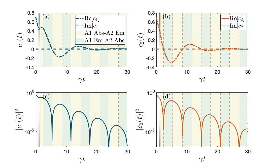
Figure 5: Dynamics of atomic coefficients (a) $c_{1}(t)$ and (b) $c_{2}(t)$, and atomic populations (c) $\left|c_{1}\left(t\right)\right|^{2}$ and (d) $\left|c_{2}\left(t\right)\right|^{2}$. Whenever the atomic coefficients change sign ($c_{1,2}(t)=0$) the atomic populations reverse their absorption and emission behavior, as indicated by the yellow and green regions corresponding to atom A1 absorbing-A2 emitting and A1 emitting-A2 absorbing, respectively.

We plot the atomic dynamics as a function of time in Fig. 5. It can be seen that when the sign of the atomic coefficients $c_{1,2}$ changes, so does the sign of its electric dipole moment that drives the field, causing the atoms to switch from absorbing to emitting, or vice versa.

Appendix C Intensity dynamics

The intensity of the field emitted by the atoms as a function of position and time can be evaluated as $I\left(x,t\right)=\frac{\epsilon_{0}c}{2}\left\langle\Psi\left(t\right)|\hat{E}^{\dagger}\left(x,t\right)\hat{E}\left(x,t\right)|\Psi\left(t\right)\right\rangle$, where $\hat{E}\left(x,t\right)=\int_{0}^{\infty}\mathrm{d}\omega\,\mathcal{E}_{\omega}\left[\hat{a}_{L}\left(\omega\right)e^{-ik_{L}x}+\hat{a}_{R}\left(\omega\right)e^{ik_{R}x}\right]e^{-i\omega t}$ is the electric field operator at position $x$ and time $t$. More explicitly, we obtain

$$I(x,t)= \frac{\epsilon_{0}c\left|\mathcal{E}_{0}\right|^{2}}{2}\left\langle\Psi\left(t\right)\right|\left[\int\mathrm{d}\omega_{1}\left\{\hat{a}_{L}^{\dagger}\left(\omega_{1}\right)e^{ik_{1L}x}+\hat{a}_{R}^{\dagger}\left(\omega_{1}\right)e^{-ik_{1R}x}\right\}e^{i\omega_{1}t}\right.$$

$$\left.\int\mathrm{d}\omega_{2}\left\{\hat{a}_{L}\left(\omega_{2}\right)e^{-ik_{2L}x}+\hat{a}_{R}\left(\omega_{2}\right)e^{ik_{2R}x}\right\}e^{-i\omega_{2}t}\right]\left|\Psi\left(t\right)\right\rangle,$$ (41)

$$= \frac{\epsilon_{0}c\left|\mathcal{E}_{0}\right|^{2}}{2}\left\langle\Psi\left(t\right)\right|\int\mathrm{d}\omega_{1}\int\mathrm{d}\omega_{2}\left[e^{i\left(k_{1L}-k_{2L}\right)x}c_{L}^{\ast}\left(\omega_{1},t\right)c_{L}\left(\omega_{2},t\right)+e^{-i\left(k_{1R}-k_{2R}\right)x}c_{R}^{\ast}\left(\omega_{1},t\right)c_{R}\left(\omega_{2},t\right)\right.$$

$$\left.+e^{-i\left(k_{1R}+k_{2L}\right)x}c_{R}^{\ast}\left(\omega_{1},t\right)c_{L}\left(\omega_{2},t\right)+e^{i\left(k_{1L}+k_{2R}\right)x}c_{L}^{\ast}\left(\omega_{1},t\right)c_{R}\left(\omega_{2},t\right)\right]e^{i\left(\omega_{1}-\omega_{2}\right)t}\left|\Psi\left(t\right)\right\rangle,$$ (42)

$$= \frac{\epsilon_{0}c\left|\mathcal{E}_{0}\right|^{2}}{2}\left\langle\Psi\left(t\right)\right|\left|\int\mathrm{d}\omega\left[c_{L}\left(\omega,t\right)e^{-i\omega x/v_{L}}+c_{R}\left(\omega,t\right)e^{i\omega x/v_{R}}\right]e^{-i\omega t}\right|^{2}\left|\Psi\left(t\right)\right\rangle,$$ (43)

$$= \frac{\epsilon_{0}c\left|\mathcal{E}_{0}\right|^{2}\gamma\beta}{4\pi}\left|\int\mathrm{d}\omega e^{-i\omega t}\left[\int_{0}^{t}\mathrm{d}\tau\left\{c_{1}\left(\tau\right)e^{i\omega(-x+x_{1})/v_{L}}+c_{2}\left(\tau\right)e^{i\omega(-x+x_{2})/v_{L}}\right.\right.\right.$$

$$\left.\left.\left.+c_{1}\left(\tau\right)e^{-i\omega(-x+x_{1})/v_{R}}+c_{2}\left(\tau\right)e^{-i\omega(-x+x_{2})/v_{R}}\right\}e^{i\left(\omega-\omega_{0}\right)\tau}\right]\right|^{2},$$ (44)

where we have used Eqs. (9) and (10) to substitute the field amplitudes in terms of the atomic excitation amplitudes. Using the W-function solution for the atomic coefficients (Eq. (27)) and performing the integrals over time and frequency, we obtain

$$I/I_{0}= \left|\sum_{\sigma=+,-}\sum_{n=-\infty}^{\infty}\left[\alpha_{n,1}^{\sigma}e^{-i\left(\omega_{0}-i\gamma_{n}^{\sigma}\right)\left(t+\left(x-x_{1}\right)/v_{L}\right)}\left\{\Theta\left[t+\left(x-x_{1}\right)/v_{L}\right]-\Theta\left[\left(x-x_{1}\right)/v_{L}\right]\right\}\right.\right.$$

$$\left.\left.+\alpha_{n,2}^{\sigma}e^{-i\left(\omega_{0}-i\gamma_{n}^{\sigma}\right)\left(t+\left(x-x_{2}\right)/v_{L}\right)}\left\{\Theta\left[t+\left(x-x_{2}\right)/v_{L}\right]-\Theta\left[\left(x-x_{2}\right)/v_{L}\right]\right\}\right.\right.$$

$$\left.\left.+\alpha_{n,1}^{\sigma}e^{-i\left(\omega_{0}-i\gamma_{n}^{\sigma}\right)\left(t-\left(x-x_{1}\right)/v_{R}\right)}\left\{\Theta\left[t-\left(x-x_{1}\right)/v_{R}\right]-\Theta\left[-\left(x-x_{1}\right)/v_{R}\right]\right\}\right.\right.$$

$$\left.\left.+\alpha_{n,2}^{\sigma}e^{-i\left(\omega_{0}-i\gamma_{n}^{\sigma}\right)\left(t-\left(x-x_{2}\right)/v_{R}\right)}\left\{\Theta\left[t-\left(x-x_{2}\right)/v_{R}\right]-\Theta\left[-\left(x-x_{2}\right)/v_{R}\right]\right\}\right]\right|^{2}.$$ (45)

We can rewrite the above in terms of the atomic excitation amplitudes using Eq. (27) as

$$I/I_{0}= \left|\left[c_{1}\left(t+\left(x+d/2\right)/v_{L}\right)e^{-i\omega_{0}\left(x+d/2\right)/v_{L}}\left\{\Theta\left[t+\left(x+d/2\right)/v_{L}\right]-\Theta\left[\left(x+d/2\right)/v_{L}\right]\right\}\right.\right.$$

$$\left.\left.+c_{2}\left(t+\left(x-d/2\right)/v_{L}\right)e^{-i\omega_{0}\left(x-d/2\right)/v_{L}}\left\{\Theta\left[t+\left(x-d/2\right)/v_{L}\right]-\Theta\left[\left(x-d/2\right)/v_{L}\right]\right\}\right.\right.$$

$$\left.\left.+c_{1}\left(t-\left(x+d/2\right)/v_{R}\right)e^{i\omega_{0}\left(x+d/2\right)/v_{R}}\left\{\Theta\left[t-\left(x+d/2\right)/v_{R}\right]-\Theta\left[-\left(x+d/2\right)/v_{R}\right]\right\}\right.\right.$$

$$\left.\left.+c_{2}\left(t-\left(x-d/2\right)/v_{R}\right)e^{i\omega_{0}\left(x-d/2\right)/v_{R}}\left\{\Theta\left[t-\left(x-d/2\right)/v_{R}\right]-\Theta\left[-\left(x-d/2\right)/v_{R}\right]\right\}\right]\right|^{2},$$ (46)

which corresponds to Eq. (6).

Appendix D Directional Emission

Let us consider the dynamics for the atomic coefficients given by Eq. (5). In the limit $\gamma T\ll 1$, neglecting the delay but keeping the propagation phases, we obtain:

$$c_{1}(t)= \left[c_{1}\left(0\right)\sum_{n=0}^{\infty}\frac{\left(\beta\frac{\gamma}{2}te^{i\phi}\right)^{2n}}{2n!}-c_{2}\left(0\right)e^{i(\phi_{L}-\phi)}\sum_{n=0}^{\infty}\frac{\left(\beta\frac{\gamma}{2}te^{i\phi}\right)^{2n+1}}{(2n+1)!}\right]e^{-\frac{\gamma}{2}t}\Theta(t),$$ (47)

$$c_{2}(t)= \left[c_{2}\left(0\right)\sum_{n=0}^{\infty}\frac{\left(\beta\frac{\gamma}{2}te^{i\phi}\right)^{2n}}{2n!}-c_{1}\left(0\right)e^{i(\phi_{R}-\phi)}\sum_{n=0}^{\infty}\frac{\left(\beta\frac{\gamma}{2}te^{i\phi}\right)^{2n+1}}{(2n+1)!}\right]e^{-\frac{\gamma}{2}t}\Theta(t).$$ (48)

These series converges to

$$c_{1}(t)= \left[c_{1}\left(0\right)\cosh\left\{\beta\frac{\gamma}{2}te^{i\phi}\right\}-c_{2}\left(0\right)e^{i(\phi_{L}-\phi)}\sinh\left\{\beta\frac{\gamma}{2}te^{i\phi}\right\}\right]e^{-\frac{\gamma}{2}t}\Theta(t),$$ (49)

$$c_{2}(t)= \left[c_{2}\left(0\right)\cosh\left\{\beta\frac{\gamma}{2}te^{i\phi}\right\}-c_{1}\left(0\right)e^{i(\phi_{R}-\phi)}\sinh\left\{\beta\frac{\gamma}{2}te^{i\phi}\right\}\right]e^{-\frac{\gamma}{2}t}\Theta(t).$$ (50)

We now consider the field coefficients in the steady state $(t\rightarrow\infty)$, which can be simplified to:

$$c_{R}(\omega,t\rightarrow\infty)=$$

$$-ig^{\ast}(\omega)e^{-i\frac{\phi_{R}}{2}}\left[\left(c_{1}\left(0\right)e^{i\phi_{R}}+c_{2}\left(0\right)\right)\frac{(\frac{\gamma}{2}-i\Delta)}{(\frac{\gamma}{2}-i\Delta)^{2}-\left(\beta\frac{\gamma}{2}e^{i\phi}\right)^{2}}-\left(c_{2}\left(0\right)e^{2i\phi}+c_{1}\left(0\right)e^{i\phi_{R}}\right)\frac{\beta\frac{\gamma}{2}}{(\frac{\gamma}{2}-i\Delta)^{2}-\left(\beta\frac{\gamma}{2}e^{i\phi}\right)^{2}}\right],$$ (51)

$$c_{L}(\omega,t\rightarrow\infty)=$$

$$-ig^{\ast}(\omega)e^{-i\frac{\phi_{L}}{2}}\left[\left(c_{1}\left(0\right)+c_{2}\left(0\right)e^{i\phi_{L}}\right)\frac{(\frac{\gamma}{2}-i\Delta)}{(\frac{\gamma}{2}-i\Delta)^{2}-\left(\beta\frac{\gamma}{2}e^{i\phi}\right)^{2}}-\left(c_{2}\left(0\right)e^{i\phi_{L}}+c_{1}\left(0\right)e^{2i\phi}\right)\frac{\beta\frac{\gamma}{2}}{(\frac{\gamma}{2}-i\Delta)^{2}-\left(\beta\frac{\gamma}{2}e^{i\phi}\right)^{2}}\right].$$ (52)

The probability of emitting the photon to the right (left) is thus given by

$$P_{R(L)}=\int_{0}^{\infty}d\omega\left|c_{R(L)}(\omega,t\rightarrow\infty)\right|^{2}.$$ (53)

We parametrize the initial atomic coefficients as $c_{1}\left(0\right)=e^{i\phi_{A1}}\cos\theta$ and $c_{2}\left(0\right)=e^{i\phi_{A2}}\sin\theta$, to obtain the right and left emission probabilities as follows:

$$P_{R}=$$

$$\left|g(\omega_{0})\right|^{2}\int_{0}^{\infty}d\omega\left|\left(\sin\theta+\cos\theta e^{i\Delta\phi}e^{i\phi}\right)\frac{(\frac{\gamma}{2}-i\Delta)}{(\frac{\gamma}{2}-i\Delta)^{2}-\left(\beta\frac{\gamma}{2}e^{i\phi}\right)^{2}}-\left(\sin\theta+\cos\theta e^{i\Delta\phi}e^{-i\phi}\right)e^{2i\phi}\frac{\beta\frac{\gamma}{2}}{(\frac{\gamma}{2}-i\Delta)^{2}-\left(\beta\frac{\gamma}{2}e^{i\phi}\right)^{2}}\right|^{2},$$ (54)

$$P_{L}=$$

$$\left|g(\omega_{0})\right|^{2}\int_{0}^{\infty}d\omega\left|\left(\sin\theta+\cos\theta e^{i\Delta\phi}e^{-i\phi}\right)\frac{(\frac{\gamma}{2}-i\Delta)}{(\frac{\gamma}{2}-i\Delta)^{2}-\left(\beta\frac{\gamma}{2}e^{i\phi}\right)^{2}}-\left(\sin\theta+\cos\theta e^{i\Delta\phi}e^{i\phi}\right)\frac{\beta\frac{\gamma}{2}}{(\frac{\gamma}{2}-i\Delta)^{2}-\left(\beta\frac{\gamma}{2}e^{i\phi}\right)^{2}}\right|^{2}.$$ (55)

We consider the integral:

$$I_{0} =\int_{0}^{\infty}d\omega\left|\frac{T_{1}(\frac{\gamma}{2}-i\Delta)-T_{2}\beta\frac{\gamma}{2}}{(\frac{\gamma}{2}-i\Delta)^{2}-\left(\beta\frac{\gamma}{2}e^{i\phi}\right)^{2}}\right|^{2},$$ (56)

$$=\left|T_{1}\right|^{2}\int_{0}^{\infty}d\omega\frac{\Delta^{2}}{\left|(\frac{\gamma}{2}-i\Delta)^{2}-\left(\beta\frac{\gamma}{2}e^{i\phi}\right)^{2}\right|^{2}}-2\mathrm{Im}\left[T_{1}T_{2}^{*}\right]\beta\frac{\gamma}{2}\int_{0}^{\infty}d\omega\frac{\Delta}{\left|(\frac{\gamma}{2}-i\Delta)^{2}-\left(\beta\frac{\gamma}{2}e^{i\phi}\right)^{2}\right|^{2}}$$

$$+\left|T_{1}-T_{2}\beta\right|^{2}\left(\frac{\gamma}{2}\right)^{2}\int_{0}^{\infty}d\omega\frac{1}{\left|(\frac{\gamma}{2}-i\Delta)^{2}-\left(\beta\frac{\gamma}{2}e^{i\phi}\right)^{2}\right|^{2}},$$

$$\equiv\left|T_{1}\right|^{2}I_{3}-2\mathrm{Im}\left[T_{1}T_{2}^{*}\right]\beta\left(\frac{\gamma}{2}\right)I_{2}+\left|T_{1}-T_{2}\beta\right|^{2}\left(\frac{\gamma}{2}\right)^{2}I_{1}.$$ (57)

where we can simplify the integrals $I_{1}$, $I_{2}$ and $I_{3}$ as follows:

$$I_{1} =\int_{0}^{\infty}d\omega\frac{1}{\left|(\frac{\gamma}{2}-i\Delta)^{2}-\left(\beta\frac{\gamma}{2}e^{i\phi}\right)^{2}\right|^{2}}=\frac{\pi}{2}\frac{1}{\left(\frac{\gamma}{2}\right)^{3}}\frac{1}{\left(1-\left(\beta\cos\phi\right)^{2}\right)\left(1+\left(\beta\sin\phi\right)^{2}\right)}$$ (58)

$$I_{2} =\int_{0}^{\infty}d\omega\frac{\Delta}{\left|(\frac{\gamma}{2}-i\Delta)^{2}-\left(\beta\frac{\gamma}{2}e^{i\phi}\right)^{2}\right|^{2}}=-\frac{\pi}{4}\frac{1}{\left(\frac{\gamma}{2}\right)^{2}}\frac{\beta^{2}\sin 2\phi}{\left(1-\left(\beta\cos\phi\right)^{2}\right)\left(1+\left(\beta\sin\phi\right)^{2}\right)},$$ (59)

$$I_{3} =\int_{0}^{\infty}d\omega\frac{\Delta^{2}}{\left|(\frac{\gamma}{2}-i\Delta)^{2}-\left(\beta\frac{\gamma}{2}e^{i\phi}\right)^{2}\right|^{2}}=\frac{\pi}{2}\frac{1}{\left(\frac{\gamma}{2}\right)}\frac{1-\beta^{2}\cos 2\phi}{\left(1-\left(\beta\cos\phi\right)^{2}\right)\left(1+\left(\beta\sin\phi\right)^{2}\right)}.$$ (60)

Substituting the above in Eq. (57), we get

$$I_{0}=\frac{\pi}{\gamma}\frac{\left|T_{1}\right|^{2}\left[1-\beta^{2}\cos 2\phi\right]+\mathrm{Im}\left[T_{1}T_{2}^{*}\right]\beta^{3}\sin 2\phi+\left|T_{1}-T_{2}\beta\right|^{2}}{\left(1-\left(\beta\cos\phi\right)^{2}\right)\left(1+\left(\beta\sin\phi\right)^{2}\right)}.$$ (61)

Plugging this result back into Eq. (D) and (D) and considering $4\pi\left|g(\omega_{0})\right|^{2}=\beta\gamma$ yields

$$P_{R}= \frac{1}{2}\frac{\beta}{1+\left(\beta\sin\phi\right)^{2}}\left[\frac{\left(1-\beta+\left(\beta\sin\phi\right)^{2}\right)\left(1-\beta\cos\Delta\phi\cos\phi\sin 2\theta\right)}{1-\left(\beta\cos\phi\right)^{2}}+\cos\left(\Delta\phi+\phi\right)\sin 2\theta+2\beta\sin^{2}\theta\sin^{2}\phi\right],$$ (62)

$$P_{L}= \frac{1}{2}\frac{\beta}{1+\left(\beta\sin\phi\right)^{2}}\left[\frac{\left(1-\beta+\left(\beta\sin\phi\right)^{2}\right)\left(1-\beta\cos\Delta\phi\cos\phi\sin 2\theta\right)}{1-\left(\beta\cos\phi\right)^{2}}+\cos\left(\Delta\phi-\phi\right)\sin 2\theta+2\beta\cos^{2}\theta\sin^{2}\phi\right].$$ (63)

which depends on the four parameters: $\beta$, $\theta$, $\phi$, and $\Delta\phi$. We use the above equations to obtain the total probability of emitting into the waveguide $P_{\mathrm{tot}}$ and the directionality parameter $\chi$ is given by Eqs. (6) and (4).

D.1 Optimum directionality

We give the parameter values that optimize the directionality parameter given by Eq. (6). The value of $\phi$ that maximizes directionality is $\phi=\frac{2n+1}{2}\pi$ such that $\sin\phi=\pm 1$. The directional parameter for the optimal value of $\phi$ reads:

$$\chi=-\frac{\sin\Delta\phi\sin 2\theta\pm\beta\cos 2\theta}{1+\beta^{2}}.$$ (64)

Considering that the value of $\beta$ is fixed for a given physical system, we find the global optimum over the two remaining parameters ($\theta$, and $\Delta\phi$), yields:

$$\beta\sin 2\theta\mp\cos 2\theta\sin\Delta\phi =0$$

$$\mp\sin 2\theta\cos\Delta\phi =0,$$

which gives the optimum values of of $\Delta\phi=\left(n+\frac{1}{2}\right)\pi$ and $\theta=\pm\frac{1}{2}\arctan\frac{1}{\beta}$. This shows that the optimum value of $\theta$ in general depends on the value of $\beta$, and it tends to $\theta\rightarrow\left(\frac{2n+1}{2}\right)\pi$ as $\beta\rightarrow 0$.

D.2 Directional Fisher Information

The directional and non-directional quantum Fisher information are defined as:

$$\mathcal{F}_{D}(\varphi)= P_{L}(\varphi)\left(\frac{\partial\log P_{L}(\varphi)}{\partial\varphi}\right)^{2}+P_{R}(\varphi)\left(\frac{\partial\log P_{R}(\varphi)}{\partial\varphi}\right)^{2}+P_{\mathrm{out}}(\varphi)\left(\frac{\partial\log P_{out}(\varphi)}{\partial\varphi}\right)^{2}$$ (65)

$$\mathcal{F}_{ND}(\varphi)= P_{\mathrm{tot}}(\varphi)\left(\frac{\partial\log P_{\mathrm{tot}}(\varphi)}{\partial\varphi}\right)^{2}+P_{\mathrm{out}}(\varphi)\left(\frac{\partial\log P_{\mathrm{out}}(\varphi)}{\partial\varphi}\right)^{2}$$ (66)

The difference between the two can be found as:

$$\mathcal{F}_{D}(\varphi)-\mathcal{F}_{ND}(\varphi) =P_{L}(\varphi)\left(\frac{\partial\log P_{L}(\varphi)}{\partial\varphi}\right)^{2}+P_{R}(\varphi)\left(\frac{\partial\log P_{R}(\varphi)}{\partial\varphi}\right)^{2}-P_{tot}(\varphi)\left(\frac{\partial\log P_{tot}(\varphi)}{\partial\varphi}\right)^{2}$$ (67)

$$=P_{L}(\varphi)\left(\frac{\partial P_{L}(\varphi)}{\partial\varphi}\frac{1}{P_{L}(\varphi)}\right)^{2}+P_{R}(\varphi)\left(\frac{\partial P_{R}(\varphi)}{\partial\varphi}\frac{1}{P_{R}(\varphi)}\right)^{2}-P_{tot}(\varphi)\left(\frac{\partial P_{tot}(\varphi)}{\partial\varphi}\frac{1}{P_{tot}(\varphi)}\right)^{2}$$ (68)

$$=\frac{1}{P_{L}(\varphi)+P_{R}(\varphi)}\left[\left(\frac{P_{R}(\varphi)}{P_{L}(\varphi)}\right)\left(\frac{\partial P_{L}(\varphi)}{\partial\varphi}\right)^{2}+\left(\frac{P_{L}(\varphi)}{P_{R}(\varphi)}\right)\left(\frac{\partial P_{R}(\varphi)}{\partial\varphi}\right)^{2}-2\frac{\partial P_{L}(\varphi)}{\partial\varphi}\frac{\partial P_{R}(\varphi)}{\partial\varphi}\right]$$ (69)

$$=\frac{1}{P_{tot}(\varphi)}\left[\left(\sqrt{\frac{P_{R}(\varphi)}{P_{L}(\varphi)}}\right)\left(\frac{\partial P_{L}(\varphi)}{\partial\varphi}\right)-\sqrt{\frac{P_{L}(\varphi)}{P_{R}(\varphi)}}\left(\frac{\partial P_{R}(\varphi)}{\partial\varphi}\right)\right]^{2}.$$ (70)

Since all the probabilities are positive real numbers, this term is always positive, thus yielding:

$$\mathcal{F}_{D}(\varphi)-\mathcal{F}_{ND}(\varphi)\geq 0.$$ (71)

The equality is satisfied when $P_{R}=P_{L}$, corresponding to equal emission probabilities in the left and right directions.

References

- Meystre [2021] P. Meystre, Quantum Optics: Taming the Quantum (Springer International Publishing, Switzerland AG, 2021).
- Predojević and Mitchell [2015] A. Predojević and M. W. Mitchell, Engineering the Atom-Photon Interaction (Springer International Publishing, New York, 2015).
- Dowling and Milburn [2003] J. P. Dowling and G. J. Milburn, Philos. Trans. Royal Soc. A 361, 1655 (2003).
- S. Haroche and J.M. Raimond [2013] S. Haroche and J.M. Raimond, Oxford University Press (2013).
- Lodahl et al. [2017] P. Lodahl, S. Mahmoodian, S. Stobbe, A. Rauschenbeutel, P. Schneeweiss, J. Volz, H. Pichler, and P. Zoller, Nature 541, 473 (2017).
- Hood et al. [2016] J. D. Hood, A. Goban, A. Asenjo-Garcia, M. Lu, S.-P. Yu, D. E. Chang, and H. J. Kimble, Proceedings of the National Academy of Sciences 113, 10507 (2016), https://www.pnas.org/content/113/38/10507.full.pdf .
- Liu and Houck [2017] Y. Liu and A. A. Houck, Nature Physics 13, 48 (2017).
- Pedersen et al. [2008] J. G. Pedersen, S. Xiao, and N. A. Mortensen, Phys. Rev. B 78, 153101 (2008).
- Asadchy et al. [2020] V. S. Asadchy, M. S. Mirmoosa, A. Díaz-Rubio, S. Fan, and S. A. Tretyakov, Proceedings of the IEEE 108, 1684 (2020).
- Jalas et al. [2013] D. Jalas, A. Petrov, M. Eich, W. Freude, S. Fan, Z. Yu, R. Baets, M. Popović, A. Melloni, J. D. Joannopoulos, M. Vanwolleghem, C. R. Doerr, and H. Renner, Nature Photonics 7, 579 (2013).
- Gross and Haroche [1982] M. Gross and S. Haroche, Phys. Rep. 93, 301 (1982).
- Dicke [1954] R. H. Dicke, Phys. Rev. 93, 99 (1954).
- Rehler and Eberly [1971] N. E. Rehler and J. H. Eberly, Phys. Rev. A 3, 1735 (1971).
- Eberly [1972] J. H. Eberly, Am. J. Phys. 40, 1374 (1972).
- Asenjo-Garcia et al. [2017] A. Asenjo-Garcia, M. Moreno-Cardoner, A. Albrecht, H. J. Kimble, and D. E. Chang, Phys. Rev. X 7, 031024 (2017).
- Needham et al. [2019] J. A. Needham, I. Lesanovsky, and B. Olmos, New J. Phys. 21, 073061 (2019).
- Skribanowitz et al. [1973] N. Skribanowitz, I. P. Herman, J. C. MacGillivray, and M. S. Feld, Phys. Rev. Lett. 30, 309 (1973).
- Pavolini et al. [1985] D. Pavolini, A. Crubellier, P. Pillet, L. Cabaret, and S. Liberman, Phys. Rev. Lett 54, 1917 (1985).
- Gross et al. [1976] M. Gross, C. Fabre, P. Pillet, and S. Haroche, Phys. Rev. Lett. 36, 1035 (1976).
- DeVoe and Brewer [1996] R. G. DeVoe and R. G. Brewer, Phys. Rev. Lett. 76, 2049 (1996).
- Scheibner et al. [2007] M. Scheibner, T. Schmidt, L. Worschech, A. Forchel, G. Bacher, T. Passow, and D. Hommel, Nat. Phys. 3, 106 (2007).
- Röhlsberger et al. [2010] R. Röhlsberger, K. Schlage1, B. Sahoo, S. Couet, and R. Rüffer, Science 328, 1248 (2010).
- Mlynek et al. [2014] J. A. Mlynek, A. A. Abdumalikov, C. Eichler, and A. Wallraff, Nat. Commun. 5, 5186 (2014).
- Goban et al. [2015] A. Goban, C.-L. Hung, J. D. Hood, S.-P. Yu, J. A. Muniz, O. Painter, and H. J. Kimble, Phys. Rev. Lett. 115, 063601 (2015).
- Guerin et al. [2016] W. Guerin, M. O. Araújo, and R. Kaiser, Phys. Rev. Lett. 116, 083601 (2016).
- Bradac et al. [2017] C. Bradac, M. T. Johnsson, M. van Breugel, B. Q. Baragiola, R. Martin, M. L. Juan, G. K. Brennen, and T. Volz, Nat. Commun. 8, 1205 (2017).
- Solano et al. [2017] P. Solano, P. Barberis-Blostein, F. K. Fatemi, L. A. Orozco, and S. L. Rolston, Nat. Commun. 8, 1857 (2017).
- Wang et al. [2020] Z. Wang, H. Li, W. Feng, X. Song, C. Song, W. Liu, Q. Guo, X. Zhang, H. Dong, D. Zheng, H. Wang, and D.-W. Wang, Phys. Rev. Lett. 124, 013601 (2020).
- Ferioli et al. [2021] G. Ferioli, A. Glicenstein, L. Henriet, I. Ferrier-Barbut, and A. Browaeys, Phys. Rev. X 11, 021031 (2021).
- Kannan et al. [2022] B. Kannan, A. Almanakly, Y. Sung, A. Di Paolo, D. A. Rower, J. Braumüller, A. Melville, B. M. Niedzielski, A. Karamlou, K. Serniak, A. Vepsäläinen, M. E. Schwartz, J. L. Yoder, R. Winik, J. I.-J. Wang, T. P. Orlando, S. Gustavsson, J. A. Grover, and W. D. Oliver, “On-demand directional photon emission using waveguide quantum electrodynamics,” (2022).
- Guimond et al. [2020] P.-O. Guimond, B. Vermersch, M. L. Juan, A. Sharafiev, G. Kirchmair, and P. Zoller, npj Quantum Information 6, 32 (2020).
- Gheeraert et al. [2020] N. Gheeraert, S. Kono, and Y. Nakamura, Phys. Rev. A 102, 053720 (2020).
- Yang et al. [2021a] X. Yang, W. Zheng, Z. Han, D. Lan, and Y. Yu, Communications in Theoretical Physics (2021a).
- Du et al. [2021] L. Du, M.-R. Cai, J.-H. Wu, Z. Wang, and Y. Li, Phys. Rev. A 103, 053701 (2021).
- Milonni [2019] P. W. Milonni, An introduction to quantum optics and quantum fluctuations (Oxford University Press, 2019).
- Meystre and Sargent [2007] P. Meystre and M. Sargent, Elements of Quantum Optics (Springer-Verlag, Berlin, 2007).
- Sinha et al. [2020a] K. Sinha, P. Meystre, E. Goldschmidt, F. K. Fatemi, S. L. Rolson, and P. Solano, Phys. Rev. Lett. 124, 043603 (2020a).
- Sinha et al. [2019] K. Sinha, P. Meystre, and P. Solano, Nanophotonic Materials, Devices, and Systems 11091, 53 (2019).
- Sinha et al. [2020b] K. Sinha, A. González-Tudela, Y. Lu, and P. Solano, Phys. Rev. A 102, 043718 (2020b).
- Dinc et al. [2019] F. Dinc, A. M. Brańczyk, and I. Ercan, Quantum 3, 213 (2019).
- Dinc and Braǹczyk [2019] F. Dinc and A. M. Braǹczyk, Phys. Rev. Research 1, 032042(R) (2019).
- Milonni and Knight [1974] P. W. Milonni and P. L. Knight, Phys. Rev. A 10, 1096 (1974).
- Longhi [2020] S. Longhi, Opt. Lett. 45, 3297 (2020).
- Calajó et al. [2019] G. Calajó, Y.-L. L. Fang, H. U. Baranger, and F. Ciccarello, Phys. Rev. Lett. 122, 073601 (2019).
- Kerckhoff et al. [2015] J. Kerckhoff, K. Lalumière, B. J. Chapman, A. Blais, and K. W. Lehnert, Phys. Rev. Applied 4, 034002 (2015).
- Wang et al. [2021] Y.-Y. Wang, S. van Geldern, T. Connolly, Y.-X. Wang, A. Shilcusky, A. McDonald, A. A. Clerk, and C. Wang, (2021), arXiv:2106.11283 [quant-ph] .
- Wang et al. [2015] Q. Wang, Z. Ouyang, M. Lin, and Q. Liu, Appl. Opt. 54, 9741 (2015).
- Huang et al. [2017] D. Huang, P. Pintus, C. Zhang, P. Morton, Y. Shoji, T. Mizumoto, and J. E. Bowers, Optica 4, 23 (2017).
- Sheremet et al. [2021] A. S. Sheremet, M. I. Petrov, I. V. Iorsh, A. V. Poshakinskiy, and A. N. Poddubny, (2021), arXiv:2103.06824 [quant-ph] .
- Masluk et al. [2012] N. A. Masluk, I. M. Pop, A. Kamal, Z. K. Minev, and M. H. Devoret, Phys. Rev. Lett. 109, 137002 (2012).
- Kuzmin et al. [2019] R. Kuzmin, N. Mehta, N. Grabon, R. Mencia, and V. E. Manucharyan, npj Quantum Information 5, 20 (2019).
- Léger et al. [2019] S. Léger, J. Puertas-Martínez, K. Bharadwaj, R. Dassonneville, J. Delaforce, F. Foroughi, V. Milchakov, L. Planat, O. Buisson, C. Naud, W. Hasch-Guichard, S. Florens, I. Snyman, and N. Roch, Nature Communications 10, 5259 (2019).
- Lama et al. [1972] W. L. Lama, R. Jodoin, and L. Mandel, American Journal of Physics 40, 32 (1972).
- Yang et al. [2021b] D. Yang, S.-h. Oh, J. Han, G. Son, J. Kim, J. Kim, M. Lee, and K. An, Nature Photonics 15, 272 (2021b).
- Zens and Rotter [2021] M. Zens and S. Rotter, Nature Photonics 15, 251 (2021).
- Kimble [2008] H. J. Kimble, Nature 453, 1023 (2008).
- Schoelkopf and Girvin [2008] R. J. Schoelkopf and S. M. Girvin, Nature 451, 664 (2008).
- Crowder et al. [2020] G. Crowder, H. Carmichael, and S. Hughes, Phys. Rev. A 101, 023807 (2020).
- Arranz Regidor et al. [2021] S. Arranz Regidor, G. Crowder, H. Carmichael, and S. Hughes, Phys. Rev. Research 3, 023030 (2021).
- Kaplan and Meystre [1981] A. E. Kaplan and P. Meystre, Opt. Lett. 6, 590 (1981).
- Kaplan and Meystre [1982] A. Kaplan and P. Meystre, Optics Communications 40, 229 (1982).
- Rosario Hamann et al. [2018] A. Rosario Hamann, C. Müller, M. Jerger, M. Zanner, J. Combes, M. Pletyukhov, M. Weides, T. M. Stace, and A. Fedorov, Phys. Rev. Lett. 121, 123601 (2018).
- Corless et al. [1996] R. M. Corless, G. H. Gonnet, D. E. G. Hare, D. J. Jeffrey, and D. E. Knuth, Adv. Comput. Math. 5, 329 (1996).