RetroGAN: A Cyclic Post-Specialization System for Improving Out-of-Knowledge and Rare Word Representations

Abstract

Retrofitting is a technique used to move word vectors closer together or further apart in their space to reflect their relationships in a Knowledge Base (KB). However, retrofitting only works on concepts that are present in that KB. RetroGAN uses a pair of Generative Adversarial Networks (GANs) to learn a one-to-one mapping between concepts and their retrofitted counterparts. It applies that mapping (post-specializes) to handle concepts that do not appear in the original KB in a manner similar to how some natural language systems handle out-of-vocabulary entries. We test our system on three word-similarity benchmarks and a downstream sentence simplification task, and achieve the state of the art (CARD-660). Altogether, our results demonstrate our system’s effectiveness for out-of-knowledge and rare word generalization.

1 Introduction

Retrofitting word embeddings with a KB Faruqui et al. (2015); Speer and Chin (2016); Mrkšić et al. (2017) means taking a vector space of word embeddings and finding a mapping that moves some of these word vectors closer together and others further apart, such that these vectors’ new positions in the vector space are in better agreement with the relationships between the same words (a.k.a., concepts) in a KB Speer and Chin (2016); Mrkšić et al. (2017). However, the retrofitting process can only work on concepts that are actually present in the KB (a.k.a., constraints), which means that retrofitting can get us improved performance in semantic tasks only on the overlapping vocabulary between the KB and the word embeddings. Post-specializationVulić et al. (2018); Kamath et al. (2019) is a solution to this problem; it is a series of techniques that try to (1) learn the mapping that retrofitting establishes and (2) generalize the mapping to the rest of the embedding vocabulary.

We develop and present a post-specialization system called RetroGAN that builds upon the approach presented as AuxGAN Ponti et al. (2018) by extending it to have a pair of Generative Adversarial Networks (GANs) Goodfellow et al. (2014). A regular GAN minimizes the loss when learning the function for post-specialization. Our pair works in a cyclic manner to minimize the losses of both the post-specialization and the inverse to ensure that there is a one-to-one mapping between the two domains. This constrains the outputs for unseen data in both domains and leads to achieving higher performance for unseen concepts.

Word	Distributional Neighbor	Retrofitted Neighbor
Dog	dog, dogs, puppy, pup , canine, pet, doggie, beagle, dachshund, cat	dog, beagle, pooch, dachshund, puppy, mutt, poodle, Rottweiler, canine, labrador
Doggo	pooch, doggies, bae, chihuahua, rad, pug, kitty, dane, furbabies, \uf602	doggies, pooch, dachshund, four-legged, Yorkie, corgi, whippet, amigos, Weimaraner, Dog

Table 1: Results of the 10 most similar embeddings for “dog” and “doggo” for FastText embeddings. The distributional neighbors are the closest embeddings in the original distributional space and the retrofitted neighbors are the closest in the RetroGAN post-specialized space. We can see that “doggo” was near slangs such as “bae” and “furbabies”, but after post-specialization, it gets closer to words that we regard as semantically similar to “dog.” The one-to-one mapping that RetroGAN provides is key to being able to incorporate useful semantic information into rare-words possibly like “doggo”.

2 Related Work

Within the field of retrofitting, work has been done in exploring the various ways of infusing constraints or KBs into word embeddings. The original work by Faruqui et al. (2015) only used synonymy relationships but not antonymy relationships, which meant that word embeddings with similar (synonymous) semantics in the KB would be pulled together, but word embeddings with dissimilar (antonymous) semantics would not be separated. The Attract-Repel work by Mrkšić et al. (2017) addressed this shortcoming by incorporating antonymy relationships in a retrofitting procedure: synonymous embeddings are attracted to each other, while antonymous embeddings are repelled against each other. This line of work was continued with the work done by Lexical Entailment Attract-Repel Vulić and Mrkšić (2018)(LEAR), which looks to add the asymmetric lexical entailment relationship to Attract-Repel.

Building on these works, a series of techniques called post-specialization were developed. These techniques consist on utilizing neural models to learn retrofitting mappings such as Glavaš and Vulić (2018) and Ponti et al. (2018); Kamath et al. (2019) which use a Deep Feed-forward Neural Network and a Generative Adversarial Network (GAN) respectively. Post-specialization permits, provided a static word embedding, to generate its retrofitted counterpart on the fly with a trained system. A concrete example is in table 1.

As it stands, attention has been shifted to using contextual embeddings such as those produced from BERT Devlin et al. (2019) on downstream tasks. Only recently have there been efforts in incorporating external, KB assertions into pre-trained transformer-based systems (e.g., KnowBERT Peters et al. (2019), Align-mask-select Ye et al. (2019), and LIBERT Lauscher et al. (2019)). LIBERT bridges contextual and retrofitted embeddings by leveraging the knowledge in retrofitted embeddings to find lexical tuples that are fed into BERT to focus on their lexical information.

GANs have been utilized extensively in the image domain to create lifelike images. CycleGAN Zhu et al. (2017) and other cyclic systems Kim et al. (2017) have been utilized to perform style transfer (i.e. apply certain distinctive characteristics from one image domain into another). CycleGAN serves to learn a, possibly unpaired, one-to-one mapping from one domain to another. To effectively utilize paired data, the work by Tripathy et al. (2018) modifies the CycleGAN architecture to include a conditional cyclic loss in which new discriminators are conditioned to determine if a generated sample is real or not based on a given, possibly paired, input. This in turn permits leveraging paired data to improve the one-to-one mapping.

3 RetroGAN

RetroGAN is a system that builds on Ponti et al. (2018) by utilizing a CycleGAN-like architecture (i.e., we use a pair of GANs cyclicly but our layers are different from the original CycleGAN). We chose the CycleGAN-like architecture because, in our domain, the cycle-consistency constraints can enforce a one-to-one mapping from original embeddings to retrofitted embeddings. This mapping guarantees that unseen concepts will have their own, unique retrofitted counterparts. We use RetroGAN to learn the mapping of Attract-Repel Mrkšić et al. (2017) retrofitting (with the synonymy and antonymy constraints from the Attract-Repel paperMrkšić et al. (2017)) on a subset of static word embeddings (i.e.., FastText Bojanowski et al. (2017), and Numberbatch Speer et al. (2017)), and perform post-specialization on the entire set.

3.1 Model & Architecture

RetroGAN consists of two GANs that interplay to balance a combination of losses to transform a particular word embedding $x_{i}\in X$ from its original domain $X$ to its counterpart $y_{i}\in Y$ in the retrofitted domain $Y$, and vice-versa. In both GANs that we employ, the generator consists of an input layer followed by 2 hidden dense layers with 2048 neurons and each followed by a dropout layer (with a percentage of 0.2 for the dropouts), and a final linear output layer with the same dimensionality as the input. The output of this layer, for the trained $G:X\rightarrow Y$ produces the post-specialized embeddings (i.e. a batch of 32 FastText embeddings produces 32 post-specialized embeddings). The hidden layers employ the ReLU Nair and Hinton (2010) activation function. Our discriminators have a similar structure (an input layer, 2 hidden layers with dropout but a percentage of 0.3), however, the second hidden layer is followed by a batch normalization layer and the output is a single neuron with a sigmoid activation. The reason for the batch normalization layer was to stabilize the training. We also utilized a third and fourth conditional discriminator following Tripathy et al. (2018), to leverage the cyclic architecture on paired data.

	Disjoint				Full
	FT-CC, A-R		FT-CC, A-R+NB		FT-CC, Attract-Repel			FT-CC, A-R+NB
Models	SL	SV	SL	SV	SL	SV	C660	SL	SV	C660
Distributional	0.4644	0.3649	0.4499	0.3643	0.4644	0.3649	0.2973	0.4499	0.3643	0.1068
Attract-Repel	0.4644	0.3649	0.4499	0.3643	0.7790	0.7632	0.3768	0.7748	0.7667	0.2203
AuxGAN	0.6127	0.4641	0.6116	0.5331	0.6901	0.5756	0.3899	0.6565	0.5872	0.2088
RetroGAN	0.6028	0.4702	0.6648	0.5971	0.7717	0.7192	0.5240	0.7960	0.7483	0.5581

Table 2: Word similarity tests results: We run two distinct scenarios in which the words present in SL and SV are present (Full) in Attract-Repel (A-R) retrofitting constraints or not (Disjoint). The Distributional row represents the results of the tests using the publicly available embeddings (FT-CC). The results are the Spearman correlation ($\rho$) between the Cosine distance of the embeddings we are evaluating and the human similarity measurements. The results for AuxGAN and RetroGAN are the average of 3 runs.

A novelty in RetroGAN is the combination of cyclic and non-cyclic optimization objectives: the regular adversarial loss for both GANs ($L_{GAN}$); the cyclic loss for both generators ($L_{CYC}$); the identity loss for both generators ($L_{ID}$); the max margin loss similar to Weston et al. (2011); Ponti et al. (2018) for both the generators and additionally for the cycle of generators ($L_{MM}$); and the conditional cycle consistency loss ($L_{cCYC}$) introduced in Tripathy et al. (2018). The combined objective has the following form:

$$\begin{split}L(G,F,D_{X},D_{Y})=L_{GAN}(G,D_{Y},X,Y)+\\ L_{GAN}(F,D_{X},X,Y)+\lambda L_{CYC}(G,F)+\\ \gamma L_{ID}(G,F,X,Y)+L_{MM}(G,F,X,Y)+\\ \varsigma L_{cCYC}(G,F,D_{cX},D_{cY},X,Y)\end{split}$$ (1)

where $G:X\rightarrow Y$ is the generator that maps the source domain $X$ of plain word embeddings to the target domain $Y$ of retrofitted word embeddings; $F:Y\rightarrow X$ is the generator that does the opposite; $D_{X}$ and $D_{Y}$ are the discriminators for the corresponding domains; and $D_{cX},D_{cY}$ are our cycle conditional discriminators. For brevity, we only go into details on $L_{MM}$ and $L_{cCYC}$. The other losses are the standard ones found in their respective works: $L_{GAN}$ is the adversarial loss from Goodfellow et al. (2014). $L_{CYC}$ is the cycle consistency loss from Zhu et al. (2017) with a scaling factor of $\lambda$ (which we set to 1); and $L_{ID}$ is the identity loss from Zhu et al. (2017), which we scale with $\gamma$ (which we set to 0.01). $L_{ID}$ serves as a check of whether the embedding is already in the correct domain. $L_{MM}$ is the max margin loss with random confounders as used by Ponti et al. (2018), and as a novel aspect, we add a cyclic margin loss:

$$\begin{split}L_{MM}(G,F,X,Y)=\Sigma^{||x||}_{i=1}\Sigma^{k}_{j=1|j\neq i}\tau[\\ (\delta_{MM}-cos(G(x_{i}),y_{i})+cos(G(x_{i}),y_{j}))+\\ (\delta_{MM}-cos(F(y_{i}),x_{i})+cos(F(y_{i}),x_{j}))+\\ \boldsymbol{(\delta_{MM}-cos(G(F(y_{i})),y_{i})+cos(G(F(y_{i})),y_{j}))}+\\ \boldsymbol{(\delta_{MM}-cos(F(G(x_{i})),x_{i})+cos(F(G(x_{i})),x_{j}))}]\end{split}$$ (2)

Equation 2, intuitively, tries to make generated embeddings similar to their gold-standard and different from confounders. RetroGAN further enforces this constraint across the cycle. Lastly, we have $L_{cCYC}$ which is the conditional cycle loss Tripathy et al. (2018), which we scale with $\varsigma$ (set to 1):

$$\begin{split}L_{cCYC}(G,F,D_{cX},D_{cY},X,Y)=\\ \mathbb{E}_{x\sim p_{data}}[log(D_{cX}(G(x),x))]+\\ \mathbb{E}_{x\sim p_{data}}[log(1-D_{cX}(G(x),F(G(x))))]+\\ \mathbb{E}_{y\sim p_{data}}[log(D_{cY}(F(y),y))]+\\ \mathbb{E}_{x\sim p_{data}}[log(1-D_{cY}(F(y),G(F(y))))]\end{split}$$ (3)

3.2 Experimental Setup

To train our system we utilize the ADAM Kingma and Ba (2015) optimizer with a learning rate of 5e-5 for the generators and 1e-4 for the non-conditional discriminators. We do not train the discriminators used in the regular GAN loss, and instead train the ones in the conditional cycle consistency loss. We also note that we did not perform explicit fine tuning of the scaling parameters, but we will do so in future work through a grid search. We train for 312,500 mini-batches which is the equivalent to the AuxGAN training, using a batch size of 32.

In our tests we use the English Common Crawl FastText with sub-word information (FT-CC) and Numberbatch 19.08 (NB) to see how performance would be affected by using embeddings that were already retrofitted with a large KB. We ran the Attract-Repel Mrkšić et al. (2017) procedure on all these embeddings then proceeded to perform our post-specialization tests on learning the mapping from FT-CC to the resulting retrofitted embeddings.

	5%			10%			25%			50%
	SL	SV	C660	SL	SV	C660	SL	SV	C660	SL	SV	C660
Attract-Repel	0.347	0.355	0.113	0.550	0.589	0.187	0.701	0.700	0.217	0.759	0.747	0.252
AuxGAN	0.615	0.510	0.453	0.667	0.569	0.470	0.679	0.581	0.475	0.685	0.600	0.490
RetroGAN	0.624	0.538	0.489	0.701	0.652	0.493	0.738	0.690	0.502	0.755	0.716	0.511

Table 3: Out of knowledge tests: We evaluate the performance of retrofitting and post specialization at varying percentages of test words seen in constraints. The full table can be seen in Appendix B

We ran the word similarity benchmarks: SimLex (SL)Hill et al. (2015) SimVerb (SV)Gerz et al. (2016), and the Cambridge Rare Word (C660) dataset Pilehvar et al. (2018). We utilize the Disjoint (evaluating words which were not seen in the constraints) and Full (evaluating words which were seen in constraints) settings from Ponti et al. (2018) for SL and SV, and evaluate C660 on the Full setting to test performance on rare words. The maximum values for the similarity benchmarks while training are listed in table 2.

We trained the publicly available AuxGAN model on 10 epochs of 1M iterations (which in AuxGAN is a single embedding pair rather than a batch of pairs) with both plain stochastic gradient descent (SGD) and ADAM (learning rate of 0.1) and selected the best performing one (ADAM) to compensate for convergence speed discrepancies. Additionally, similar to Ponti et al. (2018) we also evaluated on Light-LS Glavaš and Štajner (2015) with the default dataset Horn et al. (2014) to test downstream performance. We evaluate the accuracy of simplification substitutions(i.e., the amount of words that are substituted correctly when compared to a gold standard). We utilize the first 500k words in FT-CC and the complete Numberbatch (generating the vocabulary’s FastText embeddings as the distributional model). To test the retrofitted embeddings we substitute them in the original set.

3.3 Results & Discussion

RetroGAN outperforms AuxGAN in the majority of similarity benchmarks. We note that RetroGAN sets the state of the art on the rare-words benchmark (C660)(previously, to the best of our knowledge, it was 0.543 and 0.55 in Yang et al. (2019); Fukuda (2020)). In the similarity results for Full , we note the same observations that were noted in AuxGAN: there are some inconsistent gains and losses, which may be due to the combination of loss functions which may make the systems imprecise; although they spread the knowledge throughout the embeddings, they lose some precision when compared with the original retrofitted embeddings. The results for the lexical simplification (Light-LS) can be seen in table 4 where RetroGAN dominates.

We wanted to compare the out-of-knowledge (OOK) performance more in depth and to do this, we joined the words in SimLex (SL) and SimVerb (SV) and selected increasingly larger amounts of them ({5,10,25,50,75,100}%). We then selected the constraints that included these words, trained RetroGAN and AuxGAN with these constraints, and evaluated performance on SL, SV, and C660. Part of this can be seen in table 3. We see that RetroGAN’s performance increases every time that new constraints are added, whereas AuxGAN’s performance begins to peak after 25% of the constraints which may indicate more efficient knowledge distribution thanks to the cyclic system. Later on, the performance of RetroGAN kept increasing, but was less than the base retrofitted embeddings, possibly because of the lack of precision from the combination of losses. Lastly, we performed a small ablation study (Appendix A) on RetroGAN’s losses. We note that the max-margin loss from Ponti et al. (2018) is necessary for high performance in all the tests. We also notice that the cyclic (cyclic max-margin and cycle conditional discriminator) losses are essential for improved performance on the OOK and rare-word similarity benchmarks. We also see that the removal of the cyclic max-margin loss speeds up early learning and its addition stabilizes later learning respectively which may indicate a need to balance this. Future work will explore how to balance this losses, but it may be possible to put a scheduler to enable the loss after a peak. More details on the ablation study can be found in Appendix A.

Models	FT-CC	NB
Distributional	0.6553	0.6974
Attract-Repel	0.6993	0.6874
AuxGAN	0.7214	0.7335
RetroGAN	0.7595	0.7735

Table 4: Light-LS accuracy on Horn et al. (2014)

4 Conclusion

This work presents an improvement on post-specialization work through the use of a CycleGAN-like system called RetroGAN. We show that RetroGAN gives improved performance in both the Full (words which were seen in knowledge/constraints) and the Disjoint (words which were not seen in the constraints) evaluation settings for three benchmarks. It additionally has better performance on a downstream lexical simplification task, further confirming its improved generalization ability. We conclude that RetroGAN is an improved system for post-specializing embeddings for rare and OOK concepts.

5 Acknowledgements

This work was made possible thanks to the Media Lab Consortium funding.

Appendix A Ablation Tests

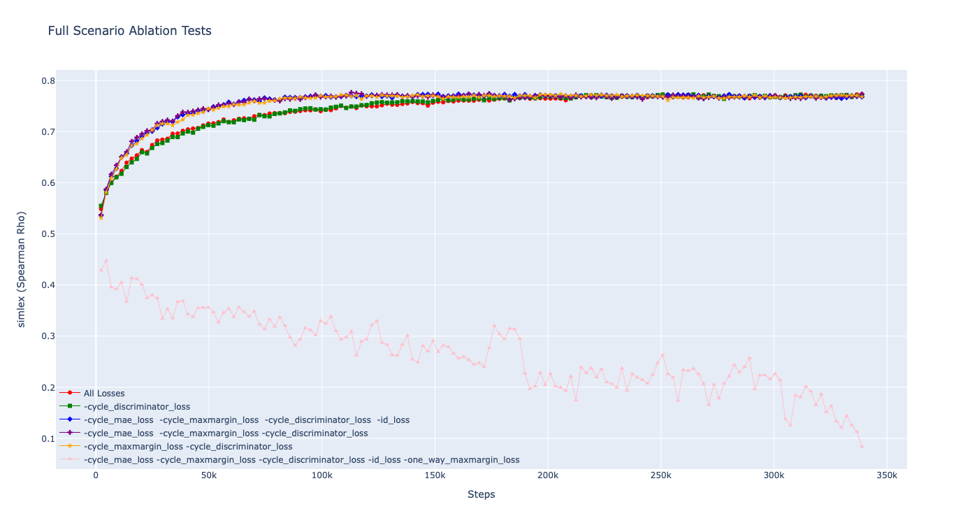
(a) SimLex Ablation Test-Full Scenario

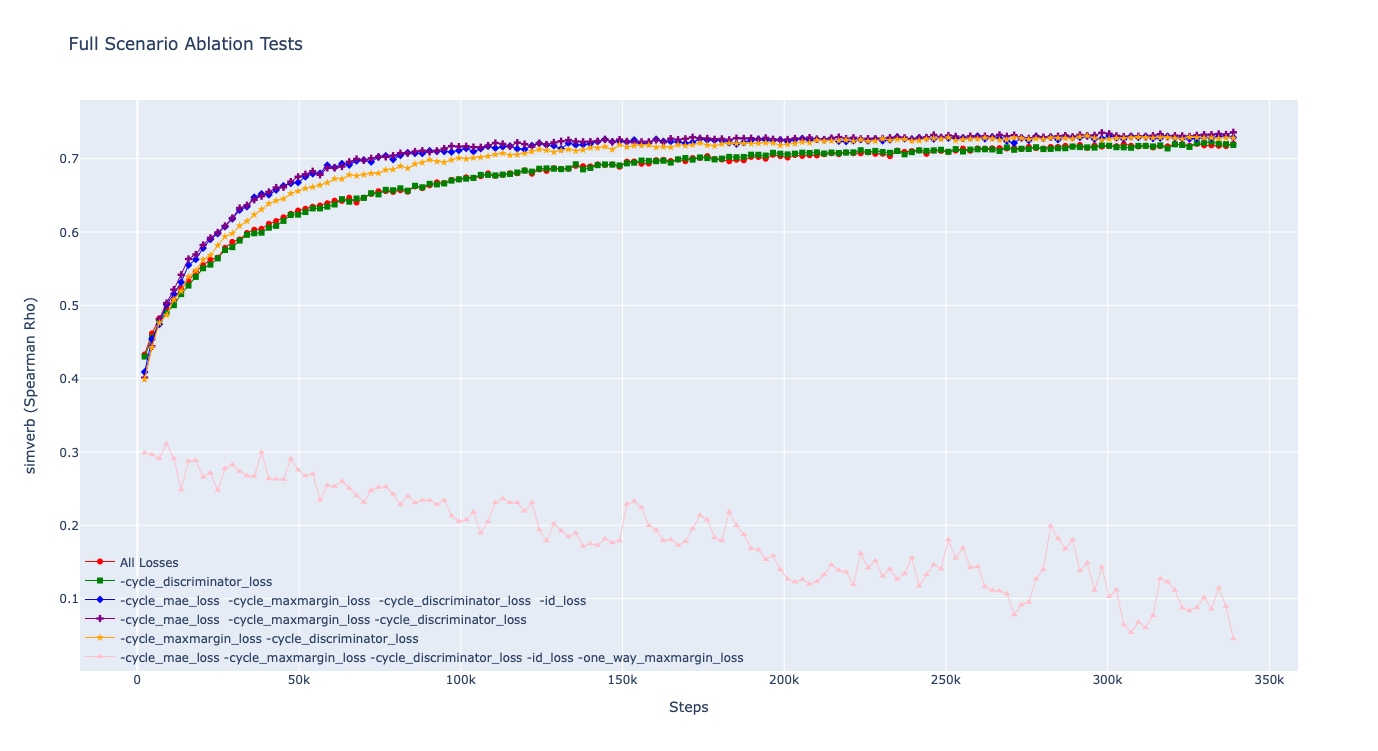
(b) SimVerb Ablation Test-Full Scenario

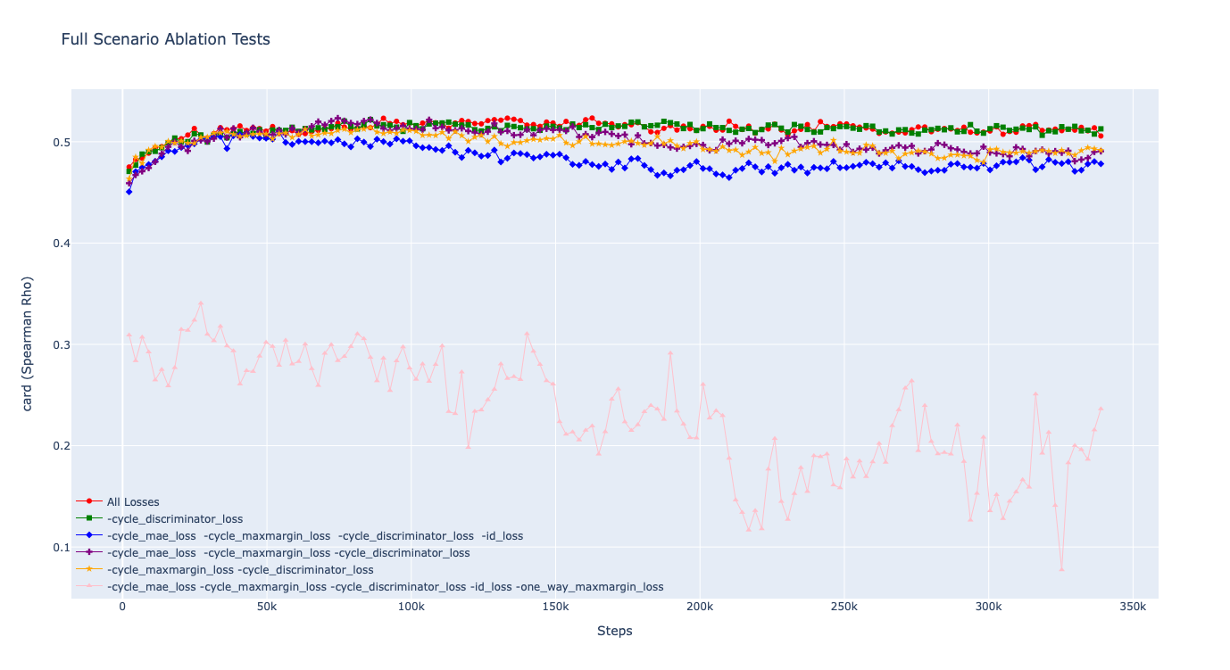
(c) CARD-660 Ablation Test-Full Scenario

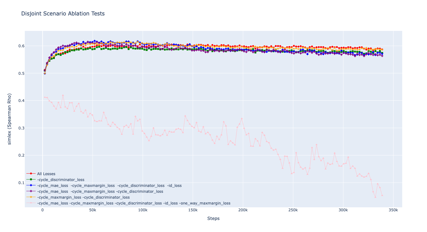
(d) SimLex Ablation Test-Disjoint Scenario

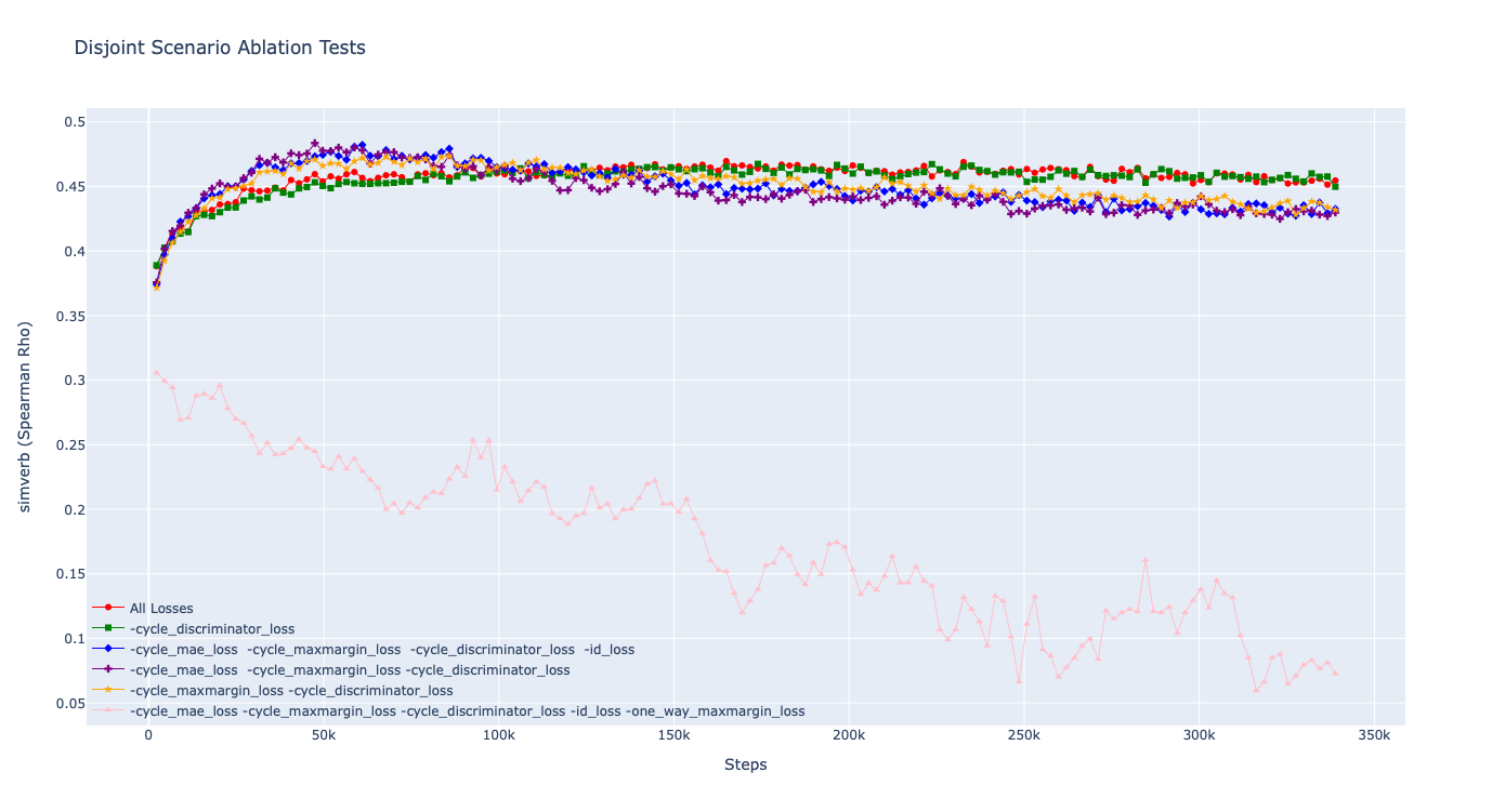
(e) SimVerb Ablation Test-Disjoint Scenario

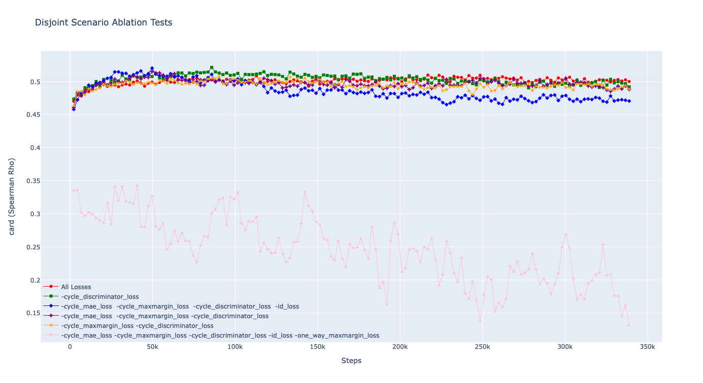
(f) CARD-660 Ablation Test-Disjoint Scenario

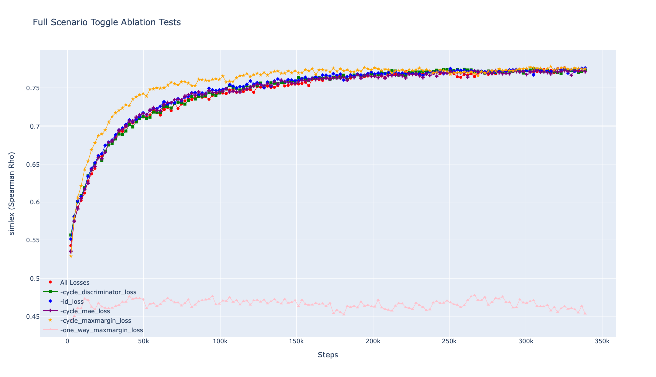
(g) SimLex Ablation Toggle Test-Disjoint Scenario

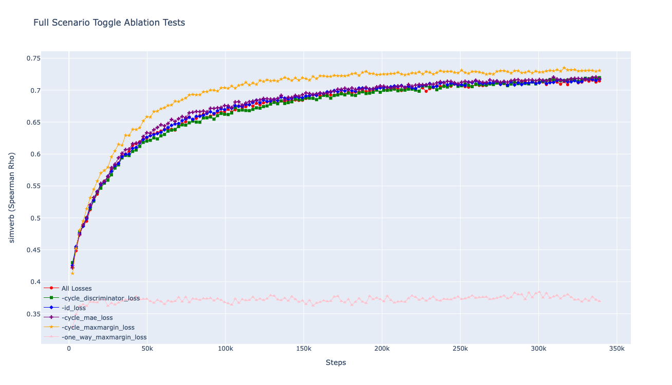
(h) SimVerb Ablation Toggle Test-Disjoint Scenario

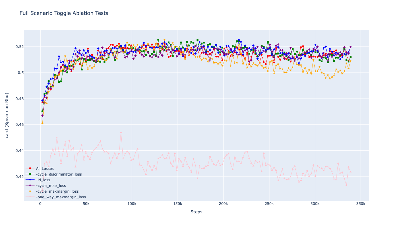
(i) CARD-660 Ablation Toggle Test-Disjoint Scenario

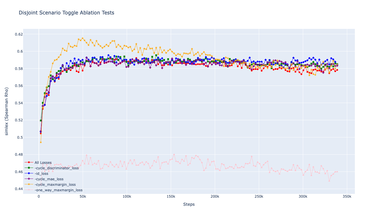
(j) SimLex Ablation Toggle Test-Disjoint Scenario

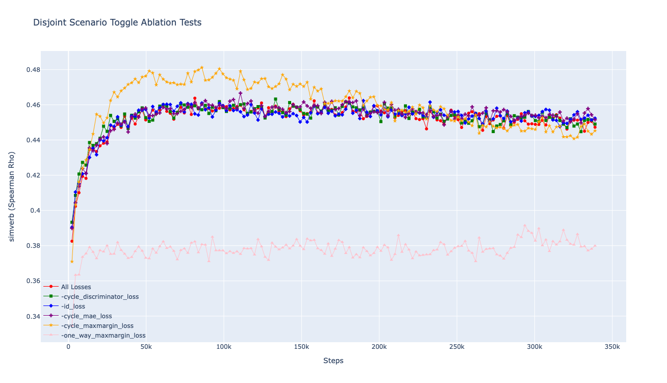
(k) SimVerb Ablation Toggle Test-Disjoint Scenario

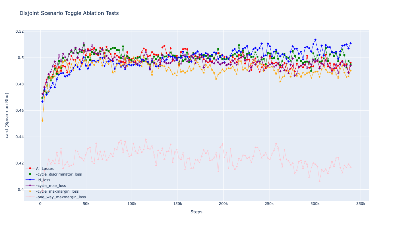
(l) CARD-660 Ablation Toggle Test-Disjoint Scenario

Figure 2: Ablation test results for SimLex, SimVerb, and CARD-660. A higher resolution version can be found in the repository at: https://github.com/pedrocolon93/retrogan.git

We performed a small ablation study to examine how the multiple losses in RetroGAN affect performance. A one-by-one removal of these can be seen in figures 2(a),2(b),2(c),2(j),2(k),2(l). A toggle of each of the losses can be seen in: 2(a),2(b),2(c),2(j),2(k),2(l). The difference between the toggle and one-by-one removal is that in the toggle, we simple turn off the specified loss and leave the others untouched, whereas in the one-by-one removal we turn off one-by-one the losses, in this way we can see the individual effects, and the group effects. We evaluated the FT-CC and the Attract-Repel retrofitted FT-CC in the same scenarios as the evaluations before (Disjoint and Full). We note that the Disjoint setting for Card includes some of the words in the constraints.

The max margin loss utilized by Ponti et al. (2018) (one_way_maxmargin_loss) is essential for high performance on the datasets. Without this loss, in all of the figures, we see that the scores in all our tests fall by at least by 0.1. This is seen in both the toggle and the one-by-one case. We can also see that the Cyclic version of this loss (cycle_maxmargin_loss) slows down learning initially, but stabilizes it in later iterations. We can see that by removing it we get higher performance in earlier iterations but the performance decays as more iterations are given. This may be because it tries to enforce that the semantic components of the embeddings be similar after going through the cycle, but it may be a hard objective to achieve. This loss is especially useful for the rare-word Card-660 evaluation. By looking at the toggle ablation test for this loss, we can see that it indeed can lead to better earlier performance, however it decays with time.

The identity loss (id_loss) helps to stabilize the training in later iterations. Removal of this loss significantly affects the disjoint settings, and the reason for it may be that it gives some indication of the important semantic components of the vectors that are being post-specialized. This in the disjoint setting leads to significant performance reductions on the later iterations. Interestingly enough, by toggling off only this loss, we can see that it leads to better performance, which means that with all the other losses, it may contain redundant information that may hinder performance, however if the model relies on the loss without other losses, its information is useful.

The Cycle Conditional discriminator loss (cycle_discriminator_loss) also contributes to the stability and generalization of the later learning. Removing this loss does not improve early learning, save on the Card-660 dataset, and in most of the other tests, there is not a large noticeable difference. However, on the disjoint setting we do see that it performance decays in later iterations. We suspect the conditioning helps slightly in the stabilization, and generalization of the system, but its effect is not too much.

The Cycle Loss (cycle_mae_loss), also stabilizes and helps in the generalization of our system. We can see in the disjoint settings in particular, that its removal hinders the model in later iterations. We suspect that since the consistency is not being enforced, the model does not learn effectively to preserve important, possibly non-semantic, parts from the distributional and the retrofitted domain.

As a practical recommendation, we suggest removing the cyclic max-margin loss either completely (pausing the training early at it’s peak around 50k-100k iterations), or toggling it after this initial training to get the speedup and the generation. Another practical recommendation may be to disable the identity loss all by itself. The other losses can be maintained as they are described in this work.

Appendix B Out-of-knowledge Scalability Tests

In table 5 we test the performance of post specialization as more constraints are added into the retrofitting process. We note that AuxGAN’s performance saturates after 50% whereas RetroGAN keeps learning, albeit less accurately than the retrofitting system. These tests were run for 100k batches on RetroGAN and for 10M iterations (312500 RetroGAN batches) on AuxGAN.

Appendix C Additional embedding pre-processing

Input and output vectors are divided by the Euclidean (2) norm. This helps slightly in the performance of the semantic comparison benchmarks. No other pre-processing is done on the vectors.

Appendix D Architecture Details

In figure 1, we can see the architecture that RetroGAN uses. On a training step, the losses are calculated as follows. For the cyclic losses, the system samples embeddings from the distributional embeddings and their retrofitted counterparts and these samples are passed to the generators (1, 5 in the figure). Then, the generators’ output is passed to the counterpart generator (Distributional Generator passes to Retrofitted Generator and vice versa, seen as 3 in the figure). The output of this is then used to calculate the max margin loss, and passed on to the subsequent discriminator to calculate the cycle discriminator loss (2, 4 in the figure). In addition to this, after going through the cycle of generators (1 or 5, 3 in the figure) we train the conditional discriminators by conditioning on real inputs from the retrofitted or distributional embeddings, or by conditioning on fake inputs (6,7 in the figure).

The amount of parameters in each model and the layers can be found in table 6.

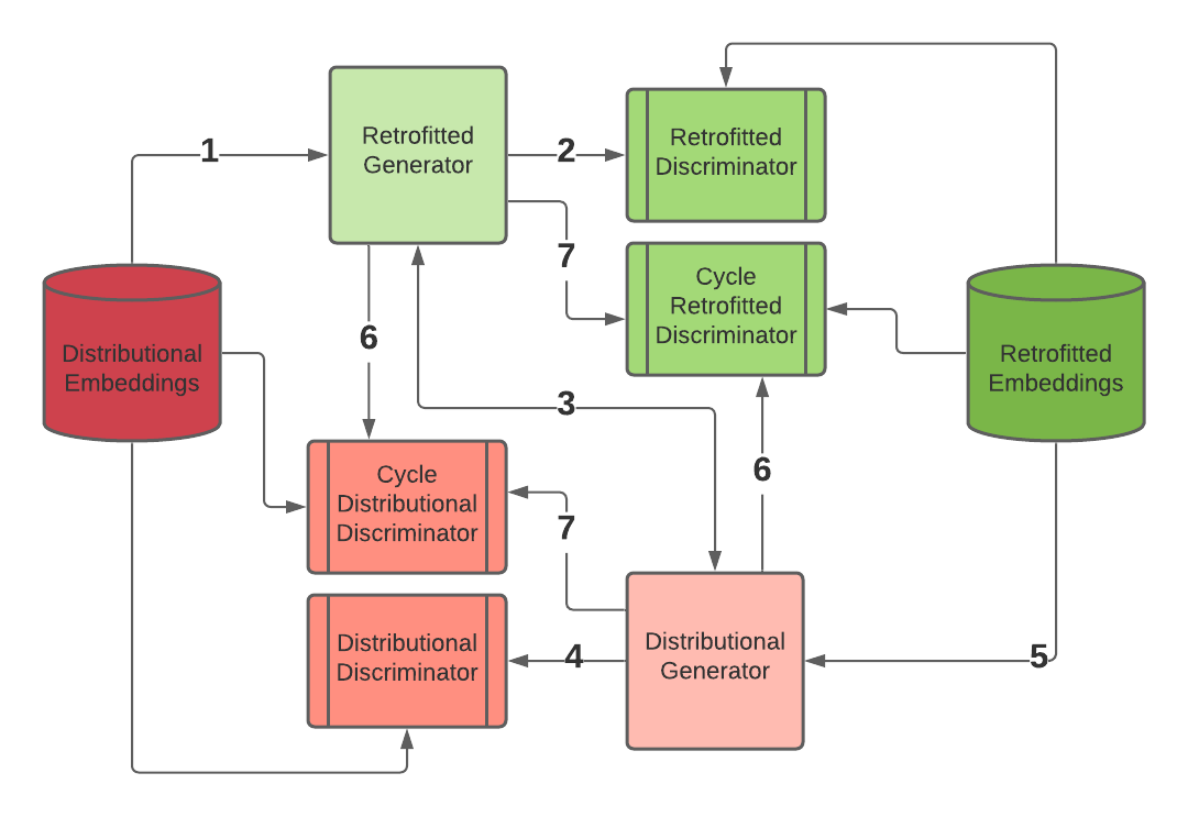
Figure 1: Architecture diagram for RetroGAN

Appendix E Parameter Tuning

We performed a parameter tuning using the Ray tuning library, to try and generate a configuration that would be optimal for RetroGAN. We utilized the ASHA SchedulerLi et al. (2020) along with the following search space configuration:

config = {
"g_lr" : tune.qloguniform(0.00005,
.1,0.00005),
"d_lr" : tune.qloguniform(0.00005,
.1,0.00005),
"one_way_mm":True,
"cycle_mm":True,
"cycle_dis":True,
"id_loss":True,
"cycle_loss":True,
"batch_size":tune.choice([16,32,64]),
"generator_size":tune.choice([512,
1024,2048]),
"discriminator_size":
tune.choice([512,1024,2048]),
"generator_hidden_layers":
tune.choice([1,2,3]),
"discriminator_hidden_layers":
tune.choice([1,2,3]),
"dis_train_amount":
tune.choice([1,2,3])
}

We used the SimVerb score to guide the parameter optimization, because it was the score that involved the largest sample of words. We also utilized a machine with two Intel processors with 48 cores in total, 128GB of RAM, an NVIDIA P6000 and a NVIDIA 1080TI. We used 25 samples in the optimization due to time constraints, although this value can be expanded more. We also ran this for 35 epochs, because the performance after that would become relatively stable and not increase greatly.

The best results from the optimization are the following:

{
’g_lr’: 0.00495,
’d_lr’: 0.00885,
’one_way_mm’: True,
’cycle_mm’: True,
’cycle_dis’: True,
’id_loss’: True,
’cycle_loss’: True,
’batch_size’: 32,
’generator_size’: 2048,
’discriminator_size’: 2048,
’generator_hidden_layers’: 1,
’discriminator_hidden_layers’: 3,
’dis_train_amount’: 1
}

	5%			10%			25%
Models	SL	SV	C660	SL	SV	C660	SL	SV	C660
Attract-Repel	0.347	0.355	0.113	0.550	0.589	0.187	0.701	0.700	0.217
AuxGAN	0.615	0.510	0.453	0.667	0.569	0.470	0.679	0.581	0.475
RetroGAN	0.624	0.538	0.489	0.701	0.652	0.493	0.738	0.690	0.502

	50%			75%			100%
Models	SL	SV	C660	SL	SV	C660	SL	SV	C660
Attract-Repel	0.759	0.747	0.252	0.766	0.757	0.244	0.771	0.761	0.257
AuxGAN	0.685	0.600	0.490	0.688	0.597	0.480	0.690	0.601	0.486
RetroGAN	0.755	0.716	0.511	0.763	0.721	0.507	0.762	0.715	0.509

Table 5: Performance of post specialization and retrofitting as more constraints are added to a system.

Model	Amount of Parameters	Layers
Generator	5,427,500(*2)	Linear (300x2048), ReLU, Dropout (0.3), Linear (2048x2048),ReLU Dropout (0.3), Linear (2048x300)
Discriminator	4,818,945(*2)	Linear (300x2048), ReLU, Dropout (0.3), Linear (2048x2048),ReLU, Batch Norm, Dropout (0.3), Linear (2048x1), Sigmoid
Cycle Conditional Discriminator	5,433,345(*2)	Linear (600x2048), ReLU, Dropout (0.3), Linear (2048x2048), ReLU, Batch Norm, Dropout (0.3), Linear (2048x1), Sigmoid
Total	31,359,580	-

Table 6: Amount of trainable parameters and layers in RetroGAN

References

- Bojanowski et al. (2017) Piotr Bojanowski, Edouard Grave, Armand Joulin, and Tomas Mikolov. 2017. Enriching word vectors with subword information. Transactions of the Association for Computational Linguistics, 5:135–146.
- Devlin et al. (2019) Jacob Devlin, Ming-Wei Chang, Kenton Lee, and Kristina Toutanova. 2019. BERT: Pre-training of deep bidirectional transformers for language understanding. In Proceedings of the 2019 Conference of the North American Chapter of the Association for Computational Linguistics: Human Language Technologies, Volume 1 (Long and Short Papers), pages 4171–4186, Minneapolis, Minnesota. Association for Computational Linguistics.
- Faruqui et al. (2015) Manaal Faruqui, Jesse Dodge, Sujay Kumar Jauhar, Chris Dyer, Eduard Hovy, and Noah A. Smith. 2015. Retrofitting word vectors to semantic lexicons. In Proceedings of the 2015 Conference of the North American Chapter of the Association for Computational Linguistics: Human Language Technologies, pages 1606–1615, Denver, Colorado. Association for Computational Linguistics.
- Fukuda (2020) Nobukazu Fukuda. 2020. Calculation of distributed representation of unknown words based on surface similarity with known words https://repository.dl.itc.u-tokyo.ac.jp/?action=repository_action_common_download&item_id=54229&item_no=1&attribute_id=14&file_no=1.
- Gerz et al. (2016) Daniela Gerz, Ivan Vulić, Felix Hill, Roi Reichart, and Anna Korhonen. 2016. SimVerb-3500: A large-scale evaluation set of verb similarity. In Proceedings of the 2016 Conference on Empirical Methods in Natural Language Processing, pages 2173–2182, Austin, Texas. Association for Computational Linguistics.
- Glavaš and Štajner (2015) Goran Glavaš and Sanja Štajner. 2015. Simplifying lexical simplification: Do we need simplified corpora? In Proceedings of the 53rd Annual Meeting of the Association for Computational Linguistics and the 7th International Joint Conference on Natural Language Processing (Volume 2: Short Papers), pages 63–68.
- Glavaš and Vulić (2018) Goran Glavaš and Ivan Vulić. 2018. Explicit retrofitting of distributional word vectors. In Proceedings of the 56th Annual Meeting of the Association for Computational Linguistics (Volume 1: Long Papers), pages 34–45.
- Goodfellow et al. (2014) Ian Goodfellow, Jean Pouget-Abadie, Mehdi Mirza, Bing Xu, David Warde-Farley, Sherjil Ozair, Aaron Courville, and Yoshua Bengio. 2014. Generative adversarial nets. In Advances in neural information processing systems, pages 2672–2680.
- Hill et al. (2015) Felix Hill, Roi Reichart, and Anna Korhonen. 2015. Simlex-999: Evaluating semantic models with (genuine) similarity estimation. Computational Linguistics, 41(4):665–695.
- Horn et al. (2014) Colby Horn, Cathryn Manduca, and David Kauchak. 2014. Learning a lexical simplifier using wikipedia. In Proceedings of the 52nd Annual Meeting of the Association for Computational Linguistics (Volume 2: Short Papers), pages 458–463.
- Kamath et al. (2019) Aishwarya Kamath, Jonas Pfeiffer, Edoardo Maria Ponti, Goran Glavaš, and Ivan Vulić. 2019. Specializing distributional vectors of all words for lexical entailment. In Proceedings of the 4th Workshop on Representation Learning for NLP (RepL4NLP-2019), pages 72–83, Florence, Italy. Association for Computational Linguistics.
- Kim et al. (2017) Taeksoo Kim, Moonsu Cha, Hyunsoo Kim, Jung Kwon Lee, and Jiwon Kim. 2017. Learning to discover cross-domain relations with generative adversarial networks. In International Conference on Machine Learning, pages 1857–1865. PMLR.
- Kingma and Ba (2015) Diederik P. Kingma and Jimmy Ba. 2015. Adam: A method for stochastic optimization. In 3rd International Conference on Learning Representations, ICLR 2015, San Diego, CA, USA, May 7-9, 2015, Conference Track Proceedings.
- Lauscher et al. (2019) Anne Lauscher, Ivan Vulić, Edoardo Maria Ponti, Anna Korhonen, and Goran Glavaš. 2019. Informing unsupervised pretraining with external linguistic knowledge. arXiv preprint arXiv:1909.02339.
- Li et al. (2020) Liam Li, Kevin Jamieson, Afshin Rostamizadeh, Ekaterina Gonina, Jonathan Ben-tzur, Moritz Hardt, Benjamin Recht, and Ameet Talwalkar. 2020. A system for massively parallel hyperparameter tuning. In Proceedings of Machine Learning and Systems, volume 2, pages 230–246.
- Mrkšić et al. (2017) Nikola Mrkšić, Ivan Vulić, Diarmuid Ó Séaghdha, Ira Leviant, Roi Reichart, Milica Gašić, Anna Korhonen, and Steve Young. 2017. Semantic specialization of distributional word vector spaces using monolingual and cross-lingual constraints. Transactions of the association for Computational Linguistics, 5:309–324.
- Nair and Hinton (2010) Vinod Nair and Geoffrey E Hinton. 2010. Rectified linear units improve restricted boltzmann machines. In Proceedings of the 27th international conference on machine learning (ICML-10), pages 807–814.
- Peters et al. (2019) Matthew E. Peters, Mark Neumann, Robert Logan, Roy Schwartz, Vidur Joshi, Sameer Singh, and Noah A. Smith. 2019. Knowledge enhanced contextual word representations. In Proceedings of the 2019 Conference on Empirical Methods in Natural Language Processing and the 9th International Joint Conference on Natural Language Processing (EMNLP-IJCNLP), pages 43–54, Hong Kong, China. Association for Computational Linguistics.
- Pilehvar et al. (2018) Mohammad Taher Pilehvar, Dimitri Kartsaklis, Victor Prokhorov, and Nigel Collier. 2018. Card-660: Cambridge rare word dataset - a reliable benchmark for infrequent word representation models. In Proceedings of the 2018 Conference on Empirical Methods in Natural Language Processing, pages 1391–1401, Brussels, Belgium. Association for Computational Linguistics.
- Ponti et al. (2018) Edoardo Maria Ponti, Ivan Vulić, Goran Glavaš, Nikola Mrkšić, and Anna Korhonen. 2018. Adversarial propagation and zero-shot cross-lingual transfer of word vector specialization. In Proceedings of the 2018 Conference on Empirical Methods in Natural Language Processing, pages 282–293, Brussels, Belgium. Association for Computational Linguistics.
- Speer and Chin (2016) Robyn Speer and Joshua Chin. 2016. An ensemble method to produce high-quality word embeddings. arXiv preprint arXiv:1604.01692.
- Speer et al. (2017) Robyn Speer, Joshua Chin, and Catherine Havasi. 2017. ConceptNet 5.5: An open multilingual graph of general knowledge. pages 4444–4451.
- Tripathy et al. (2018) Soumya Tripathy, Juho Kannala, and Esa Rahtu. 2018. Learning image-to-image translation using paired and unpaired training samples. In Asian Conference on Computer Vision, pages 51–66. Springer.
- Vulić et al. (2018) Ivan Vulić, Goran Glavaš, Nikola Mrkšić, and Anna Korhonen. 2018. Post-specialisation: Retrofitting vectors of words unseen in lexical resources. In Proceedings of the 2018 Conference of the North American Chapter of the Association for Computational Linguistics: Human Language Technologies, Volume 1 (Long Papers), pages 516–527, New Orleans, Louisiana. Association for Computational Linguistics.
- Vulić and Mrkšić (2018) Ivan Vulić and Nikola Mrkšić. 2018. Specialising word vectors for lexical entailment. In Proceedings of the 2018 Conference of the North American Chapter of the Association for Computational Linguistics: Human Language Technologies, Volume 1 (Long Papers), pages 1134–1145, New Orleans, Louisiana. Association for Computational Linguistics.
- Weston et al. (2011) Jason Weston, Samy Bengio, and Nicolas Usunier. 2011. Wsabie: Scaling up to large vocabulary image annotation. In Twenty-Second International Joint Conference on Artificial Intelligence.
- Yang et al. (2019) Ziyi Yang, Chenguang Zhu, Vin Sachidananda, and Eric Darve. 2019. Out-of-vocabulary embedding imputation with grounded language information by graph convolutional networks. arXiv e-prints, pages arXiv–1906.
- Ye et al. (2019) Zhi-Xiu Ye, Qian Chen, Wen Wang, and Zhen-Hua Ling. 2019. Align, mask and select: A simple method for incorporating commonsense knowledge into language representation models. arXiv preprint arXiv:1908.06725.
- Zhu et al. (2017) Jun-Yan Zhu, Taesung Park, Phillip Isola, and Alexei A Efros. 2017. Unpaired image-to-image translation using cycle-consistent adversarial networks. In Proceedings of the IEEE international conference on computer vision, pages 2223–2232.