Kolmogorov’s dissipation number and determining wavenumber for dyadic models

Abstract.

We study some dyadic models for incompressible magnetohydrodynamics and Navier-Stokes equation. The existence of fixed point and stability of the fixed point are established. The scaling law of Kolmogorov’s dissipation wavenumber arises from heuristic analysis. In addition, a time-dependent determining wavenumber is shown to exist; moreover, the time average of the determining wavenumber is proved to be bounded above by Kolmogorov’s dissipation wavenumber. Additionally, based on the knowledge of the fixed point and stability of the fixed point, numerical simulations are performed to illustrate the energy spectrum in the inertial range below Kolmogorov’s dissipation wavenumber.

KEY WORDS: dyadic models; intermittency; fixed point; dissipation wavenumber; determining wavenumber.

CLASSIFICATION CODE: 35Q35, 76D03, 76W05.

1. Introduction

As a primary model in geophysics and astrophysics, the incompressible magnetohydrodynamics (MHD) system

$$\begin{split}u_{t}+u\cdot\nabla u-B\cdot\nabla B+\nabla p=&\ \nu\Delta u,\\ B_{t}+u\cdot\nabla B-B\cdot\nabla u=&\ \mu\Delta B,\\ \nabla\cdot u=0,\ \ \nabla\cdot B=&\ 0,\end{split}$$ (1.1)

has been extensively studied both in physics and mathematics literatures. In the equations, the vector fields $u$ and $B$ denote respectively the fluid velocity and magnetic field; the scalar function $p$ represents the pressure; the parameters $\nu$ and $\mu$ stand for the kinematic viscosity and magnetic resistivity respectively. When $B\equiv 0$, system (1.1) reduces to the Navier-Stokes equation (NSE)

$$\begin{split}u_{t}+u\cdot\nabla u+\nabla p=&\ \nu\Delta u,\\ \nabla\cdot u=&\ 0,\end{split}$$ (1.2)

which has been a central objective in the area of fluid dynamics.

Although being studied for a long time, there are still peculiar behaviours of solutions to (1.1) and (1.2) which remain mysteries. The nonlinearities within the systems stir up complexities in the energy cascade mechanism of the dynamics. In the history, many attempts to better understand the pure fluid system (1.2) involve studying approximating systems of (1.2). Notably, a class of dyadic models of (1.2) have been proposed and well studied, see [1, 2, 4, 7, 8, 12, 15, 16, 19, 20, 21] (which is certainly not a complete list). Dyadic models for MHD have appeared and been studied mainly numerically in physics literature, see [3, 17], the survey paper [22] and references therein. Recently, dyadic models for MHD were also proposed within the umbrella of harmonic analysis techniques in [10] by the first author. The intermittency dimension $\delta$, introduced in term of the saturation of Bernstein’s inequality [5], is naturally included in the modeling process.

In this paper, we focus on two particular dyadic models suggested in [10] for the MHD with external forcing, one with only forward energy cascade given by

$$\begin{split}\frac{d}{dt}a_{j}+\nu\lambda_{j}^{2}a_{j}=&\ \lambda_{j-1}^{\theta}a_{j-1}^{2}-\lambda_{j}^{\theta}a_{j}a_{j+1}+\lambda_{j-1}^{\theta}b_{j-1}^{2}-\lambda_{j}^{\theta}b_{j}b_{j+1}+f_{j},\\ \frac{d}{dt}b_{j}+\mu\lambda_{j}^{2}b_{j}=&\ \lambda_{j}^{\theta}a_{j}b_{j+1}-\lambda_{j}^{\theta}b_{j}a_{j+1}\end{split}$$ (1.3)

for $j\geq 0$ and $a_{-1}=b_{-1}=0$; and another with both forward and backward energy cascades,

$$\begin{split}\frac{d}{dt}a_{j}+\nu\lambda_{j}^{2}a_{j}=&\ \lambda_{j-1}^{\theta}a_{j-1}^{2}-\lambda_{j}^{\theta}a_{j}a_{j+1}-\lambda_{j-1}^{\theta}b_{j-1}^{2}+\lambda_{j}^{\theta}b_{j}b_{j+1}+f_{j},\\ \frac{d}{dt}b_{j}+\mu\lambda_{j}^{2}b_{j}=&-\lambda_{j}^{\theta}a_{j}b_{j+1}+\lambda_{j}^{\theta}b_{j}a_{j+1}.\end{split}$$ (1.4)

The parameter $\theta$ is given by

$$\theta=\frac{2+n-\delta}{2}\in\left[1,\frac{2+n}{2}\right],\ \ \ \delta\in[0,n]$$

with $\delta$ being the intermittency dimension of the $n$-dimensional velocity field $u$ and magnetic field $B$, which are assumed to be the same. If $b_{j}\equiv 0$ for all $j\geq 0$, both models (1.3) and (1.4) reduce to a forced dyadic model for the NSE (1.2),

$$\frac{d}{dt}a_{j}+\nu\lambda_{j}^{2}a_{j}=\lambda_{j-1}^{\theta}a_{j-1}^{2}-\lambda_{j}^{\theta}a_{j}a_{j+1}+f_{j},\ \ \ j\geq 0$$ (1.5)

with $a_{-1}=0$, which is equipped with a forward energy cascade mechanism. For system (1.3) with $\nu=\mu=0$, the total energy defined by

$$E(t)=\frac{1}{2}\sum_{j\geq 1}\left(a_{j}^{2}(t)+b_{j}^{2}(t)\right)$$

is formally conserved; however, the cross helicity defined by

$$H^{c}(t)=\sum_{j\geq 1}a_{j}(t)b_{j}(t)$$

is not conserved, accompanied with the mechanism of only forward energy cascade. While both the total energy and cross helicity are invariant for system (1.4) with $\nu=\mu=0$.

The dyadic NSE model (1.5) has been understood comprehensively. Without external forcing, it was shown in [4] that: starting from nonnegative initial data, strong solution exists globally in time when $\theta\leq 2$ and solution blows up at finite time when $\theta>3$. Later the authors of [1] proved the existence of global strong solution of (1.5) with zero forcing when $\theta\leq\frac{5}{2}$. In [7], assuming non-zero forcing only on the first mode, the authors proved the existence of a unique fixed point for (1.5); furthermore, they showed the fixed point is a global attractor and it converges to the global attractor of the inviscid system as $\nu\to 0$. In these findings, the preservation of positivity of solutions play vital roles. With an external forcing, uniqueness of Leray-Hopf solution was established for (1.5) with $\theta\leq 2$ in [13, 14]; and non-unique Leray-Hopf solutions were constructed for (1.5) with $\theta>2$ in [14].

As a contrast, the dyadic MHD models (1.3) and (1.4) are much harder to be analyzed compared to the NSE model (1.5). Obviously, the interactions between the velocity components $a_{j}$ and magnetic field components $b_{j}$ cause obstacles to understand energy transfer from shell to shell. Moreover, due to such interactions, it is not clear whether a solution of (1.3) or (1.4) with positive initial data stays positive for all the time or not; and it is possible that a solution starting from positive initial data may become negative. Without the conservation of positivity of a solution, many techniques and methods for the dyadic NSE model fail to work for models (1.3) and (1.4). Nevertheless, with the lack of positivity, the authors of [11] proved existence and uniqueness of Leray-Hopf solution for (1.3) and (1.4) with $\theta\leq 2$ and appropriate forcing; they also constructed non-unique Leray-Hopf solutions for (1.3) and (1.4) with $\theta>2$ and a particular forcing term. Assuming positivity, it was shown in [9] that positive solution of (1.3) with large initial data blows up at finite time when $\theta>3$.

The main objective of this paper is to study large time behaviours of solutions to (1.3) and (1.4) in the following means. We first show the existence of fixed point and study the stability of the fixed point under assumption of either small forcing or small initial perturbation. In analogy with Kolmogorov’s turbulence theory for hydrodynamics [18], we then perform heuristic scaling analysis for the dyadic MHD models to indicate the existence of critical kinetic dissipation wavenumber $\kappa_{\mathrm{d}}^{u}$ and critical magnetic dissipation wavenumber $\kappa_{\mathrm{d}}^{b}$, with the former separating the kinetic inertial range from the kinetic dissipation range and the latter separating the ion-inertial range from the magnetic dissipation range. Below the critical wavenumber $\kappa_{\mathrm{d}}^{u}$ and $\kappa_{\mathrm{d}}^{b}$, we predict the scaling of the kinetic energy spectrum $\mathcal{E}_{u}(k)$ and magnetic energy spectrum $\mathcal{E}_{b}(k)$ respectively. Furthermore, we establish the existence of time-dependent determining wavenumber $\lambda_{J}$ in the sense: if two weak solutions in the energy space are close to each other below $\lambda_{J}$, the two solutions are asymptotically identical in the energy space. Both point-wise and time average estimates for the determining wavenumber $\lambda_{J}$ will be obtained. Notably, we show that the time average of $\lambda_{J}$ is bounded above by the dissipation wavenumber $\kappa_{\mathrm{d}}^{u}$ and $\kappa_{\mathrm{d}}^{b}$. It thus provides theoretical ground for the heuristic scaling law of $\kappa_{\mathrm{d}}^{u}$ and $\kappa_{\mathrm{d}}^{b}$. In the end, based on the knowledge of the fixed point and stability results established earlier, we design numerical scheme to simulate the dyadic models. The numerical results confirm the predicted scaling law of the energy spectra $\mathcal{E}_{u}(k)$ and $\mathcal{E}_{b}(k)$.

We note that the dyadic NSE model (1.5) is a reduced system of both (1.3) and (1.4). Thus the results described in the last paragraph for the dyadic MHD models can be obtained for (1.5) with some modifications.

2. Preliminaries

We denote $H=l^{2}$ which is endowed with the standard scalar product and norm,

$$(u,v):=\sum_{n=1}^{\infty}u_{n}v_{n},\ \ \ |u|:=\sqrt{(u,u)}.$$

As mentioned earlier, we choose the wavenumber $\lambda_{n}=\lambda^{n}$ for a constant $\lambda>1$, and all integers $n\geq 0$. As standard Sobolev space $H^{s}$ for functions with spacial variables, we use the same notation $H^{s}$ in this paper to represent the space for a sequence $\{u_{n}\}_{n=1}^{\infty}$, which is endowed with the scaler product

$$(u,v)_{s}:=\sum_{n=1}^{\infty}\lambda_{n}^{2s}u_{n}v_{n}$$

and the norm

$$\|u\|_{s}:=\sqrt{(u,u)_{s}}.$$

Notice that $H^{0}=l^{2}$ is the energy space.

We introduce the concept of solutions for dyadic models as follows.

Definition 2.1.

A pair of $H$-valued functions $(a(t),b(t))$ defined on $[t_{0},\infty)$ is said to be a weak solution of (1.3) if $a_{j}$ and $b_{j}$ satisfy (1.3) and $a_{j},b_{j}\in C^{1}([t_{0},\infty))$ for all $j\geq 0$.

Definition 2.2.

A solution $(a(t),b(t))$ of (1.3) is strong on $[T_{1},T_{2}]$ if $\|a\|_{1}$ and $\|b\|_{1}$ are bounded on $[T_{1},T_{2}]$. A solution is strong on $[T_{1},\infty)$ if it is strong on every interval $[T_{1},T_{2}]$ for any $T_{2}>T_{1}$.

Definition 2.3.

A Leray-Hopf solution $(a(t),b(t))$ of (1.3) on $[t_{0},\infty)$ is a weak solution satisfying the energy inequality

$$|a(t)|^{2}+|b(t)|^{2}+2\nu\int_{t_{1}}^{t}\|a(\tau)\|_{1}\,d\tau+2\mu\int_{t_{1}}^{t}\|b(\tau)\|_{1}\,d\tau\leq|a(t_{1})|^{2}+|b(t_{1})|^{2}$$

for all $t_{0}\leq t_{1}\leq t$ and a.e. $t_{1}\in[t_{0},\infty)$.

Solutions of (1.4) and (1.5) are defined in the same way.

Definition 2.4.

(Lyapunov stability) The system

$$x^{\prime}(t)=f(x),\ \ x(t_{0})=x_{0}$$

is said to be stable in the sense of Lyapunov with respect to the fixed point $x^{*}$, if for any $\varepsilon>0$, there exists a constant $\delta=\delta(\varepsilon,t_{0})>0$ such that

$$|x(t)-x^{*}|<\varepsilon,\ \ \ \forall\ \ t\geq t_{0}\ \ \mbox{provided}\ \ |x(t_{0})-x^{*}|<\delta.$$

3. Fixed point

3.1. Existence of fixed point and properties of fixed point

We consider the stationary system of (1.3) with

$$\frac{d}{dt}a_{j}=\frac{d}{dt}b_{j}=0,\ \ \forall j\geq 0,$$

$$f_{0}>0;\ \ f_{j}=0,\ \forall j\geq 1$$

Define the rescaled quantities

$$A_{j}=\lambda^{-\frac{1}{6}\theta}f_{0}^{-\frac{1}{2}}\lambda_{j}^{\frac{1}{3}\theta}a_{j},\ \ \ B_{j}=\lambda^{-\frac{1}{6}\theta}f_{0}^{-\frac{1}{2}}\lambda_{j}^{\frac{1}{3}\theta}b_{j},$$

$$\bar{\nu}=\nu\lambda^{\frac{1}{6}\theta}f_{0}^{-\frac{1}{2}},\ \ \ \bar{\mu}=\mu\lambda^{\frac{1}{6}\theta}f_{0}^{-\frac{1}{2}}.$$

The stationary system of (1.3) can be written as

$$\begin{split}A_{j-1}^{2}-A_{j}A_{j+1}+B_{j-1}^{2}-B_{j}B_{j+1}=&\ \bar{\nu}\lambda_{j}^{2-\frac{2}{3}\theta}A_{j},\ \ j\geq 1,\\ A_{j}B_{j+1}-B_{j}A_{j+1}=&\ \bar{\mu}\lambda_{j}^{2-\frac{2}{3}\theta}B_{j},\ \ j\geq 1,\\ -A_{0}A_{1}-B_{0}B_{1}=&\ \bar{\nu}A_{0}-1,\\ A_{0}B_{1}-B_{0}A_{1}=&\ \bar{\mu}B_{0}.\end{split}$$ (3.6)

Theorem 3.1.

There exists a fixed point $(a^{*},b^{*})\in\ell^{2}\times\ell^{2}$ to (1.3). Equivalently, there exists a solution $\{(A_{j},B_{j})\}$ to (3.6) with $(A,B)\in H^{-\frac{1}{3}\theta}\times H^{-\frac{1}{3}\theta}$.

Proof: It is sufficient to show the existence of an absorbing ball for (1.3). Consequently, the existence of solutions to the stationary system follows from standard fixed point arguments, for instance, an application of Brouwer’s fixed point theorem.

To make the following argument rigorous, one can apply it to Galerkin approximating systems and pass to the limit. Formally, multiplying $a_{j}$ to the first equation of (1.3), $b_{j}$ to the second one, adding the resulted equations, and taking sum over $j\geq 1$ gives us the a priori energy estimate,

$$\begin{split}\frac{d}{dt}\left(\|a\|_{2}^{2}+\|b\|_{2}^{2}\right)\leq&\ -2\nu\sum_{j=0}^{\infty}\lambda_{j}^{2}a_{j}^{2}-2\mu\sum_{j=0}^{\infty}\lambda_{j}^{2}b_{j}^{2}+\sum_{j=0}^{\infty}a_{j}f_{j}\\ \leq&\ -2m_{0}\lambda_{0}^{2}\left(\|a\|_{2}^{2}+\|b\|_{2}^{2}\right)+m_{0}\lambda_{0}^{2}\|a\|_{2}^{2}+(m_{0}\lambda_{0}^{2})^{-1}\|f\|_{2}^{2}\\ \leq&\ -m_{0}\lambda_{0}^{2}\left(\|a\|_{2}^{2}+\|b\|_{2}^{2}\right)+(m_{0}\lambda_{0}^{2})^{-1}\|f\|_{2}^{2}\end{split}$$

where $m_{0}=\min\{\nu,\mu\}$. It follows from the energy estimate that

$$\frac{d}{dt}\left(\|a\|_{2}^{2}+\|b\|_{2}^{2}\right)<0,\ \ \mbox{if}\ \ \|a\|_{2}^{2}+\|b\|_{2}^{2}>(m_{0}\lambda_{0}^{2})^{-2}\|f\|_{2}^{2}.$$

Thus, there exists an absorbing ball in the energy space $\ell^{2}\times\ell^{2}$ with radius
$(m_{0}\lambda_{0}^{2})^{-1}\|f\|_{2}$.

$\Box$

Remark 3.2.

We note $(a^{*},b^{*})$ is a Leray-Hopf solution. By Leray structure theory, we know every Leray-Hopf solution is regular almost everywhere in time. Since $(a^{*},b^{*})$ is stationary, it is thus regular everywhere and hence belongs to $H^{s}\times H^{s}$ for any $s>0$. Consequently, the solution $(A,B)$ of (3.6) is in fact in $H^{s}\times H^{s}$ for any $s>0$ as well.

Lemma 3.3.

Let $(A,B)$ be a solution to (3.6). Then we have either

$$A_{j}>0,\ \ B_{j}>0,\ \ \ \forall\ \ j\geq 0,$$

or

$$A_{j}>0,\ \ B_{j}<0,\ \ \ \forall\ \ j\geq 0.$$

Proof: Denote $(\ref{stat-2-gen})_{i}$ by the $i$-th equation of system (3.6) for $1\leq i\leq 4$. Multiplying equation $(\ref{stat-2-gen})_{1}$ by $A_{j}$, $(\ref{stat-2-gen})_{2}$ by $B_{j}$, $(\ref{stat-2-gen})_{3}$ by $A_{0}$ and $(\ref{stat-2-gen})_{4}$ by $B_{0}$, and taking sum for $j\geq 0$, we obtain

$$\sum_{j=0}^{\infty}\lambda_{j}^{2-\frac{2}{3}\theta}\left(\bar{\nu}A_{j}^{2}+\bar{\mu}B_{j}^{2}\right)=A_{0}.$$

Since $(A,B)\in H^{s}\times H^{s}$ for any $s>0$, the sum on the left hand side of the equation above is well-defined. If instead taking sum for $j\geq J$ with $J\geq 0$, we have

$$\sum_{j=J}^{\infty}\lambda_{j}^{2-\frac{2}{3}\theta}\left(\bar{\nu}A_{j}^{2}+\bar{\mu}B_{j}^{2}\right)=\left(A_{J-1}^{2}+B_{J-1}^{2}\right)A_{J}.$$

Thus we claim $A_{j}>0$ for all $j\geq 0$.

The equations $(\ref{stat-2-gen})_{2}$ and $(\ref{stat-2-gen})_{4}$ imply

$$\begin{split}B_{j+1}=&\ \frac{\bar{\mu}\lambda_{j}^{2-\frac{2}{3}\theta}+A_{j+1}}{A_{j}}B_{j},\ \ \forall\ \ j\geq 1,\\ B_{1}=&\ \frac{\bar{\mu}+A_{1}}{A_{0}}B_{0}.\end{split}$$

Since $A_{j}>0$ for all $j\geq 0$, we have if $B_{0}>0$, then $B_{j}>0$ for all $j\geq 0$; or if $B_{0}<0$, then $B_{j}<0$ for all $j\geq 0$.

$\Box$

In the case of the inviscid non-resistive dyadic MHD model, i.e. $\nu=\mu=0$ in (1.3), we are able to derive an exact form of the fixed point, which will be used to provide the last mode for the truncated system in our numerical simulation. The stationary system (3.6) becomes

$$\begin{split}A_{j-1}^{2}-A_{j}A_{j+1}+B_{j-1}^{2}-B_{j}B_{j+1}=&\ 0,\ \ j\geq 1,\\ A_{j}B_{j+1}-B_{j}A_{j+1}=&\ 0,\ \ j\geq 1,\\ -A_{0}A_{1}-B_{0}B_{1}=&-1,\\ A_{0}B_{1}-B_{0}A_{1}=&\ 0.\end{split}$$ (3.7)

Lemma 3.4.

[11] The solutions $\{(A_{j},B_{j})\}$ of (3.7) satisfy

$$A_{j}=A_{0},\ \ B_{j}=B_{0},\ \ \forall\ \ j\geq 1,$$

$$A_{0}^{2}+B_{0}^{2}=1.$$

3.2. Stability of fixed point

In this part, we show that a fixed point of (1.3) is stable under certain conditions. Specifically, we will establish the following results: (i) when the force $f_{0}$ is small or $\mu$ and $\nu$ are large enough, the fixed point is exponentially stable and thus unique; (ii) solutions starting from initial data that is closed to a fixed point converge to the fixed point, that is, the fixed point is stable in the sense of Lyapunov.

Theorem 3.5.

Solutions of system (1.3) with $\theta\leq 2$ and $0<f_{0}<\frac{1}{8}m_{0}^{2}$ converge to a fixed point in $\ell^{2}\times\ell^{2}$. Consequently, the fixed point is unique.

Proof: Let $(a(t),b(t))$ be a solution of (1.3). Denote the difference with the fixed point by

$$u(t)=a(t)-a^{*},\ \ \ v(t)=b(t)-b^{*}.$$

The difference $(u,v)$ satisfies the system

$$\begin{split}\frac{d}{dt}u_{j}=&\ -\nu\lambda_{j}^{2}u_{j}-\lambda_{j}^{\theta}u_{j}u_{j+1}+\lambda_{j-1}^{\theta}u_{j-1}^{2}-\lambda_{j}^{\theta}v_{j}v_{j+1}+\lambda_{j-1}^{\theta}v_{j-1}^{2}\\ &-\lambda_{j}^{\theta}u_{j}a_{j+1}^{*}-\lambda_{j}^{\theta}a_{j}^{*}u_{j+1}+2\lambda_{j-1}^{\theta}u_{j-1}a_{j-1}^{*}\\ &-\lambda_{j}^{\theta}v_{j}b_{j+1}^{*}-\lambda_{j}^{\theta}b_{j}^{*}v_{j+1}+2\lambda_{j-1}^{\theta}v_{j-1}b_{j-1}^{*},\\ \frac{d}{dt}v_{j}=&\ -\mu\lambda_{j}^{2}v_{j}+\lambda_{j}^{\theta}u_{j}v_{j+1}-\lambda_{j}^{\theta}v_{j}u_{j+1}\\ &+\lambda_{j}^{\theta}u_{j}b_{j+1}^{*}+\lambda_{j}^{\theta}a_{j}^{*}v_{j+1}-\lambda_{j}^{\theta}v_{j}a_{j+1}^{*}-\lambda_{j}^{\theta}b_{j}^{*}u_{j+1}.\end{split}$$ (3.8)

Multiplying $(\ref{eq-diff})_{1}$ by $u_{j}$ and $(\ref{eq-diff})_{2}$ by $v_{j}$, taking sum for $0\leq j\leq k$ with arbitrary $k\geq 1$, we get

$$\begin{split}\frac{1}{2}\frac{d}{dt}\sum_{j=0}^{k}\left(u_{j}^{2}+v_{j}^{2}\right)=&\ -\sum_{j=0}^{k}\left(\nu\lambda_{j}^{2}u_{j}^{2}+\mu\lambda_{j}^{2}v_{j}^{2}\right)-\sum_{j=0}^{k}\lambda_{j}^{\theta}\left(u_{j}^{2}+v_{j}^{2}\right)a_{j+1}^{*}\\ &+2\sum_{j=0}^{k}\lambda_{j-1}^{\theta}u_{j-1}u_{j}a_{j-1}^{*}-\sum_{j=0}^{k}\lambda_{j}^{\theta}u_{j}u_{j+1}a_{j}^{*}\\ &+2\sum_{j=0}^{k}\lambda_{j-1}^{\theta}v_{j-1}u_{j}b_{j-1}^{*}-\sum_{j=0}^{k}\lambda_{j}^{\theta}v_{j}u_{j+1}b_{j}^{*}\\ &-\sum_{j=0}^{k}\lambda_{j}^{\theta}u_{j}v_{j+1}b_{j}^{*}+\sum_{j=0}^{k}\lambda_{j}^{\theta}v_{j}v_{j+1}a_{j}^{*}\\ &-\lambda_{k}^{\theta}u_{k}^{2}u_{k+1}-\lambda_{k}^{\theta}v_{k}^{2}u_{k+1}.\end{split}$$

Since $(a^{*},b^{*})\in H^{s}\times H^{s}$ for any $s>0$, $\lambda_{j}^{s}a_{j}^{*}\to 0$ and $\lambda_{j}^{s}b_{j}^{*}\to 0$ as $j\to\infty$. We also note that $\sum_{j=0}^{\infty}\lambda_{j}^{2}u_{j}^{2}$ and $\sum_{j=0}^{\infty}\lambda_{j}^{2}v_{j}^{2}$ are integrable. Hence, taking $k\to\infty$ in the equation above and applying the dominated convergence theorem, we deduce

$$\begin{split}&\frac{1}{2}\sum_{j=0}^{\infty}\left(u_{j}^{2}(t)+v_{j}^{2}(t)\right)-\frac{1}{2}\sum_{j=0}^{\infty}\left(u_{j}^{2}(0)+v_{j}^{2}(0)\right)\\ &+\int_{0}^{t}\sum_{j=0}^{\infty}\left(\nu\lambda_{j}^{2}u_{j}^{2}(\tau)+\mu\lambda_{j}^{2}v_{j}^{2}(\tau)\right)\,d\tau\\ \leq&-\int_{0}^{t}\sum_{j=0}^{\infty}\lambda_{j}^{\theta}\left(u_{j}^{2}(\tau)+v_{j}^{2}(\tau)\right)a_{j+1}^{*}\,d\tau\\ &+\int_{0}^{t}\sum_{j=0}^{\infty}\lambda_{j}^{\theta}u_{j}(\tau)u_{j+1}(\tau)a_{j}^{*}\,d\tau+\int_{0}^{t}\sum_{j=0}^{\infty}\lambda_{j}^{\theta}v_{j}(\tau)u_{j+1}(\tau)b_{j}^{*}\,d\tau\\ &-\int_{0}^{t}\sum_{j=0}^{\infty}\lambda_{j}^{\theta}u_{j}(\tau)v_{j+1}(\tau)b_{j}^{*}\,d\tau+\int_{0}^{t}\sum_{j=0}^{\infty}\lambda_{j}^{\theta}v_{j}(\tau)v_{j+1}(\tau)a_{j}^{*}\,d\tau.\end{split}$$ (3.9)

From the proof of Theorem 3.1, we realize that the fixed point lies in an absorbing ball with radius $m_{0}^{-1}\lambda_{0}^{-2}\|f\|_{2}=(\min\{\nu,\mu\})^{-1}f_{0}$ in $\ell^{2}\times\ell^{2}$. It follows that

$$\|a^{*}\|_{2}^{2}+\|b^{*}\|_{2}^{2}\leq\min\{\nu,\mu\}^{-2}f_{0}^{2},$$

and hence

$$|a_{j}^{*}|\leq(\min\{\nu,\mu\})^{-1}f_{0},\ \ \ |b_{j}^{*}|\leq(\min\{\nu,\mu\})^{-1}f_{0},\ \ \ \forall\ \ j\geq 0.$$ (3.10)

Applying (3.10), we have

$$\begin{split}-\int_{0}^{t}\sum_{j=0}^{\infty}\lambda_{j}^{\theta}\left(u_{j}^{2}(\tau)+v_{j}^{2}(\tau)\right)a_{j+1}^{*}\,d\tau\leq m_{0}^{-1}f_{0}\int_{0}^{t}\sum_{j=0}^{\infty}\lambda_{j}^{\theta}\left(u_{j}^{2}(\tau)+v_{j}^{2}(\tau)\right)\,d\tau,\end{split}$$ (3.11)

$$\begin{split}\int_{0}^{t}\sum_{j=0}^{\infty}\lambda_{j}^{\theta}u_{j}(\tau)u_{j+1}(\tau)a_{j}^{*}\,d\tau\leq m_{0}^{-1}f_{0}\int_{0}^{t}\sum_{j=0}^{\infty}\lambda_{j}^{\theta}u_{j}^{2}(\tau)\,d\tau,\end{split}$$ (3.12)

$$\begin{split}\int_{0}^{t}\sum_{j=0}^{\infty}\lambda_{j}^{\theta}v_{j}(\tau)u_{j+1}(\tau)b_{j}^{*}\,d\tau\leq m_{0}^{-1}f_{0}\int_{0}^{t}\sum_{j=0}^{\infty}\lambda_{j}^{\theta}\left(u_{j}^{2}(\tau)+v_{j}^{2}(\tau)\right)\,d\tau,\end{split}$$ (3.13)

$$\begin{split}-\int_{0}^{t}\sum_{j=0}^{\infty}\lambda_{j}^{\theta}u_{j}(\tau)v_{j+1}(\tau)b_{j}^{*}\,d\tau\leq m_{0}^{-1}f_{0}\int_{0}^{t}\sum_{j=0}^{\infty}\lambda_{j}^{\theta}\left(u_{j}^{2}(\tau)+v_{j}^{2}(\tau)\right)\,d\tau,\end{split}$$ (3.14)

$$\begin{split}\int_{0}^{t}\sum_{j=0}^{\infty}\lambda_{j}^{\theta}v_{j}(\tau)v_{j+1}(\tau)a_{j}^{*}\,d\tau\leq m_{0}^{-1}f_{0}\int_{0}^{t}\sum_{j=0}^{\infty}\lambda_{j}^{\theta}v_{j}^{2}(\tau)\,d\tau.\end{split}$$ (3.15)

Combining (3.9) and (3.11)-(3.15), we infer

$$\begin{split}&\sum_{j=0}^{\infty}\left(u_{j}^{2}(t)+v_{j}^{2}(t)\right)-\sum_{j=0}^{\infty}\left(u_{j}^{2}(0)+v_{j}^{2}(0)\right)\\ \leq&\ -2m_{0}\int_{0}^{t}\sum_{j=0}^{\infty}\lambda_{j}^{2}\left(u_{j}^{2}(\tau)+v_{j}^{2}(\tau)\right)\,d\tau\\ &+8m_{0}^{-1}f_{0}\int_{0}^{t}\sum_{j=0}^{\infty}\lambda_{j}^{\theta}\left(u_{j}^{2}(\tau)+v_{j}^{2}(\tau)\right)\,d\tau.\end{split}$$ (3.16)

If $\theta\leq 2$ and $0<f_{0}<\frac{1}{8}m_{0}^{2}$, inequality (3.16) implies

$$\begin{split}&\sum_{j=0}^{\infty}\left(u_{j}^{2}(t)+v_{j}^{2}(t)\right)-\sum_{j=0}^{\infty}\left(u_{j}^{2}(0)+v_{j}^{2}(0)\right)\\ \leq&\ -m_{0}\int_{0}^{t}\sum_{j=0}^{\infty}\lambda_{j}^{2}\left(u_{j}^{2}(\tau)+v_{j}^{2}(\tau)\right)\,d\tau\\ \leq&\ -m_{0}\int_{0}^{t}\sum_{j=0}^{\infty}\left(u_{j}^{2}(\tau)+v_{j}^{2}(\tau)\right)\,d\tau.\end{split}$$ (3.17)

Employing Grönwall’s integral inequality to (3.17), we obtain

$$\sum_{j=0}^{\infty}\left(u_{j}^{2}(t)+v_{j}^{2}(t)\right)\leq e^{-m_{0}t}\sum_{j=0}^{\infty}\left(u_{j}^{2}(0)+v_{j}^{2}(0)\right).$$

It indicates that

$$(u(t),v(t))\to 0\ \ \ \mbox{as}\ \ t\to\infty\ \ \mbox{in}\ \ \ell^{2}\times\ell^{2},$$

and hence

$$(a(t),b(t))\to(a^{*},b^{*})\ \ \ \mbox{as}\ \ t\to\infty\ \ \mbox{in}\ \ \ell^{2}\times\ell^{2}.$$

$\Box$

Theorem 3.6.

(Lyapunov Stability) Let $(a(t),b(t))$ be a solution to (1.3) with initial data $(a_{0},b_{0})$ on $[0,T]$. For any $\varepsilon>0$, there exists a constant $\delta>0$ such that

$$\|a(t)-a^{*}\|_{2}^{2}+\|b(t)-b^{*}\|_{2}^{2}\leq\varepsilon,\ \ \ \forall\ \ 0\leq t\leq T,$$

provided

$$\|a_{0}-a^{*}\|_{2}^{2}+\|b_{0}-b^{*}\|_{2}^{2}\leq\delta.$$

Proof: A slight modification of the proof of Theorem 3.5 is sufficient to justify the statement. We start from the energy estimate (3.9) established earlier. Instead of (3.10), applying the fact that $\lambda_{j}^{s}a_{j}^{*}\to 0$ and $\lambda_{j}^{s}b_{j}^{*}\to 0$ as $j\to\infty$ for any $s>0$ we know there exists $J>0$ such that

$$\lambda_{j}^{\theta-2}a^{*}_{j}<\frac{m_{0}}{36},\ \ \lambda_{j}^{\theta-2}b^{*}_{j}<\frac{m_{0}}{36},\ \ \forall\ \ j>J.$$ (3.18)

Denote

$$C_{1}=8\lambda_{J}^{\theta}\sup_{0\leq j\leq J+1}\left(\|a^{*}_{j}\|_{L^{\infty}}+\|b^{*}_{j}\|_{L^{\infty}}\right).$$

Employing (3.18), we estimate the high modes part of the right hand side of (3.9) as follows

$$\begin{split}-\int_{0}^{t}\sum_{j=J+1}^{\infty}\lambda_{j}^{\theta}\left(u_{j}^{2}(\tau)+v_{j}^{2}(\tau)\right)a_{j+1}^{*}\,d\tau\leq\frac{m_{0}}{36}\int_{0}^{t}\sum_{j=J+1}^{\infty}\lambda_{j}^{2}\left(u_{j}^{2}(\tau)+v_{j}^{2}(\tau)\right)\,d\tau,\end{split}$$

$$\begin{split}\int_{0}^{t}\sum_{j=J+1}^{\infty}\lambda_{j}^{\theta}u_{j}(\tau)u_{j+1}(\tau)a_{j}^{*}\,d\tau\leq\frac{m_{0}}{36}\int_{0}^{t}\sum_{j=J+1}^{\infty}\lambda_{j}^{2}u_{j}^{2}(\tau)\,d\tau,\end{split}$$

$$\begin{split}\int_{0}^{t}\sum_{j=J+1}^{\infty}\lambda_{j}^{\theta}v_{j}(\tau)u_{j+1}(\tau)b_{j}^{*}\,d\tau\leq\frac{m_{0}}{36}\int_{0}^{t}\sum_{j=J+1}^{\infty}\lambda_{j}^{2}\left(u_{j}^{2}(\tau)+v_{j}^{2}(\tau)\right)\,d\tau,\end{split}$$

$$\begin{split}-\int_{0}^{t}\sum_{j=J+1}^{\infty}\lambda_{j}^{\theta}u_{j}(\tau)v_{j+1}(\tau)b_{j}^{*}\,d\tau\leq\frac{m_{0}}{36}\int_{0}^{t}\sum_{j=J+1}^{\infty}\lambda_{j}^{2}\left(u_{j}^{2}(\tau)+v_{j}^{2}(\tau)\right)\,d\tau,\end{split}$$

$$\begin{split}\int_{0}^{t}\sum_{j=J+1}^{\infty}\lambda_{j}^{\theta}v_{j}(\tau)v_{j+1}(\tau)a_{j}^{*}\,d\tau\leq\frac{m_{0}}{36}\int_{0}^{t}\sum_{j=J+1}^{\infty}\lambda_{j}^{2}v_{j}^{2}(\tau)\,d\tau.\end{split}$$

While the low modes part of the right hand side of (3.9) satisfies

$$\begin{split}&-\int_{0}^{t}\sum_{j=0}^{J}\lambda_{j}^{\theta}\left(u_{j}^{2}(\tau)+v_{j}^{2}(\tau)\right)a_{j+1}^{*}\,d\tau\\ &+\int_{0}^{t}\sum_{j=0}^{J}\lambda_{j}^{\theta}u_{j}(\tau)u_{j+1}(\tau)a_{j}^{*}\,d\tau+\int_{0}^{t}\sum_{j=0}^{J}\lambda_{j}^{\theta}v_{j}(\tau)u_{j+1}(\tau)b_{j}^{*}\,d\tau\\ &-\int_{0}^{t}\sum_{j=0}^{J}\lambda_{j}^{\theta}u_{j}(\tau)v_{j+1}(\tau)b_{j}^{*}\,d\tau+\int_{0}^{t}\sum_{j=0}^{J}\lambda_{j}^{\theta}v_{j}(\tau)v_{j+1}(\tau)a_{j}^{*}\,d\tau\\ \leq&\ C_{1}\int_{0}^{t}\sum_{j=0}^{J}\left(u_{j}^{2}(\tau)+v_{j}^{2}(\tau)\right)\,d\tau.\end{split}$$

As a consequence, it follows from (3.9) that

$$\begin{split}&\frac{1}{2}\sum_{j=0}^{\infty}\left(u_{j}^{2}(t)+v_{j}^{2}(t)\right)-\frac{1}{2}\sum_{j=0}^{\infty}\left(u_{j}^{2}(0)+v_{j}^{2}(0)\right)\\ \leq&\ -\frac{1}{2}m_{0}\int_{0}^{t}\sum_{j=0}^{\infty}\left(\lambda_{j}^{2}u_{j}^{2}(\tau)+\lambda_{j}^{2}v_{j}^{2}(\tau)\right)\,d\tau+C_{1}\int_{0}^{t}\sum_{j=0}^{J}\left(u_{j}^{2}(\tau)+v_{j}^{2}(\tau)\right)\,d\tau.\end{split}$$ (3.19)

Applying Grönwall’s inequality to (3.19) we obtain

$$\sum_{j=0}^{\infty}\left(u_{j}^{2}(t)+v_{j}^{2}(t)\right)\leq e^{2C_{1}t}\sum_{j=0}^{\infty}\left(u_{j}^{2}(0)+v_{j}^{2}(0)\right).$$

The statement of the theorem follows immediately.

$\Box$

4. Analogue of Kolmogorov’s turbulence theory

Denote $\varepsilon=\nu\langle\|\nabla u\|_{L^{2}}^{2}\rangle$ by the average energy dissipation rate per unit mass. The zeroth law of turbulence on anomalous energy dissipation postulates that $\varepsilon$ does not converge to 0 as $\nu\to 0$. On this ground, Kolmogorov [18] proposed a theory for homogeneous isotropic turbulence under the assumption of self-similarity of the flow. The two major predictions are stated below.

Conjecture 4.1.

(Kolmogorov’s predictions)
(i) There exists a critical wavenumber $\kappa_{\mathrm{d}}\sim(\varepsilon\nu^{-3})^{\frac{1}{4}}$ for the 3D flow such that only the low frequency part below $\kappa_{\mathrm{d}}$ is essential to describe the flow.
(ii) The energy density spectrum has the form

$$\mathcal{E}(k)\sim\varepsilon^{2/3}k^{-5/3}$$

for wavenumber $k$ below $\kappa_{\mathrm{d}}$ and in the viscosity limit $\nu\to 0$.

The critical wavenumber $\kappa_{\mathrm{d}}$ is often referred as Kolmogorov’s dissipation wavenumber, which separates the inertial range and dissipation range. Kolmogorov’s work was attained by using statistical tools and scaling analysis. Part (i) says that the linear term $\nu\Delta u$ dominates the nonlinear effect above $\kappa_{\mathrm{d}}$. Part (ii) gives a quantitative description of the distribution of energy in frequency domain in the inertial range. There are enormous experimental support for the predictions. Only until recent, the first author and collaborators [5, 6] gave the first rigorous mathematical justification of part (i) in the average sense.

Kolmogorov’s phenomenological theory for hydrodynamics was derived under the assumption of homogeneity, isotropy and self-similarity on the flow. However, experiments suggest that a fully developed turbulent flow may be spatially and temporally inhomogeneous, which is termed as the intermittent nature. In a general principle, intermittency is characterized as a deviation from Kolmogorov’s predictions.

In the recent work [5], we gave a mathematical definition of intermittency dimension $\delta$ of a flow through Bernstein’s inequality. For 3D flow, $\delta$ belongs to $[0,3]$. The general formulation of both Kolmogorov’s dissipation wavenumber and the energy spectrum by taking into account the intermittency effect was provided as well in [5]. Kolmogorov’s theory corresponds to the extreme intermittency regime $\delta=3$, in which turbulent eddies fill the space.

The main purpose of this section is to derive scaling laws for energy spectrum, structure functions, and the critical dissipation wavenumber that separates the inertial range from the dissipation range, for the energy forward cascade dyadic model (1.3). Numerical simulation results in Section 8 are employed to confirm these scaling laws.

Denote the average dissipation rate of the kinetic energy by $\varepsilon_{u}=\nu\left<\lambda_{j}^{2}a_{j}^{2}\right>$ and the kinetic energy spectrum by $\mathcal{E}_{u}(\lambda_{j})=\left<a_{j}^{2}\right>/\lambda_{j}$; and similarly $\varepsilon_{b}=\mu\left<\lambda_{j}^{2}b_{j}^{2}\right>$ the average dissipation rate of the magnetic energy and $\mathcal{E}_{b}(\lambda_{j})=\left<b_{j}^{2}\right>/\lambda_{j}$ the magnetic energy spectrum.

Conjecture 4.2.

The kinetic energy spectrum of the dyadic MHD system (1.3) in the kinetic inertial range separated from the kinetic dissipation range by the dissipation wavenumber

$$\kappa_{\mathrm{d}}^{u}\sim(\nu^{-3}\varepsilon_{u})^{\frac{1}{\delta+1}}$$

exhibits the scaling

$$\mathcal{E}_{u}(k)\sim\varepsilon_{u}^{\frac{2}{3}}k^{\frac{\delta-8}{3}};$$

while the magnetic energy spectrum satisfies

$$\mathcal{E}_{b}(k)\sim\varepsilon_{b}^{\frac{2}{3}}k^{\frac{\delta-8}{3}}$$

in the ion-inertial range below the magnetic dissipation wavenumber

$$\kappa_{\mathrm{d}}^{b}\sim\left(\mu^{-3}\varepsilon_{b}\right)^{\frac{1}{\delta+1}}.$$

Heuristic Motivation of Conjecture 4.2: Below is the heuristic analysis to obtain the predictions above. According to the $a_{j}$ equation of dyadic MHD model (1.3), a balance between the kinetic nonlinearity and dissipation indicates

$$\lambda_{j}^{\frac{5-\delta}{2}}a_{j}a_{j+1}\sim\nu\lambda_{j}^{2}a_{j},$$

which implies

$$a_{j+1}\sim\nu\lambda_{j}^{\frac{\delta-1}{2}}\sim\nu\lambda_{j+1}^{\frac{\delta-1}{2}}.$$ (4.20)

It then follows from (4.20) that the kinetic energy dissipation rate of the $j$-th shell satisfies

$$\varepsilon_{u,j}:=\nu\lambda_{j}^{2}a_{j}^{2}\sim\nu^{3}\lambda_{j}^{\delta+1}.$$

It indicates that $\lambda_{j}\sim(\nu^{-3}\varepsilon_{u,j})^{1/(\delta+1)}$ needs to be satisfied in order to have comparable nonlinear kinetic effect and dissipation effect, which is the motivation of the scale of the dissipation wavenumber $\kappa_{\mathrm{d}}^{u}$. Moreover, it implies $\nu\sim(\varepsilon_{u,j}\lambda_{j}^{-\delta-1})^{\frac{1}{3}}$, which along with (4.20) indicates that

$$\mathcal{E}_{u}(\lambda_{j})\sim\frac{a_{j}^{2}}{\lambda_{j}}\sim\nu^{2}\lambda_{j}^{\delta-2}\sim\left(\varepsilon_{u,j}\lambda_{j}^{-\delta-1}\right)^{\frac{2}{3}}\lambda_{j}^{\delta-2}\sim\varepsilon_{u,j}^{\frac{2}{3}}\lambda_{j}^{\frac{\delta-8}{3}}.$$

Thus, the scaling of $\mathcal{E}_{u}$ in the conjecture follows immediately.

On the other hand, assuming a balance between the magnetic dissipation and the coupled nonlinear term in the equation of $b_{j}$ of (1.3), we infer

$$\mu\lambda_{j}^{2}b_{j}\sim\lambda_{j}^{\frac{5-\delta}{2}}b_{j}a_{j+1}\Longrightarrow a_{j+1}\sim\mu\lambda_{j}^{\frac{\delta-1}{2}}.$$

While the balance between the dissipation and the magnetic nonlinearity in the $a_{j}$ equation of (1.3) yields

$$\nu\lambda_{j}^{2}a_{j}\sim\lambda_{j}^{\frac{5-\delta}{2}}b_{j}b_{j+1}\Longrightarrow b_{j}b_{j+1}\sim\nu\lambda_{j}^{\frac{\delta-1}{2}}a_{j}\sim\nu\mu\lambda_{j}^{\delta-1}.$$

Providing $b_{j}\sim b_{j+1}$, the above result gives rise to

$$b_{j}^{2}\sim\nu\mu\lambda_{j}^{\delta-1}.$$ (4.21)

It then follows

$$\varepsilon_{b,j}:=\mu\lambda_{j}^{2}b_{j}^{2}\sim\nu\mu^{2}\lambda_{j}^{\delta+1}.$$ (4.22)

Recalling $\nu\sim\varepsilon_{u,j}^{\frac{1}{3}}\lambda_{j}^{-\frac{\delta+1}{3}}$, we have from (4.22)

$$\mu\sim(\nu^{-1}\varepsilon_{b,j})^{\frac{1}{2}}\lambda_{j}^{-\frac{1}{2}(\delta+1)}\sim\varepsilon_{u,j}^{-\frac{1}{6}}\varepsilon_{b,j}^{\frac{1}{2}}\lambda_{j}^{-\frac{1}{3}\delta-\frac{1}{3}}.$$ (4.23)

Finally, we postulate from (4.21) and (4.23)

$$\begin{split}\mathcal{E}_{b}(\lambda_{j})\sim&\ b_{j}^{2}/\lambda_{j}\sim\nu\mu\lambda_{j}^{\delta-2}\sim\varepsilon_{u,j}^{\frac{1}{6}}\varepsilon_{b,j}^{\frac{1}{2}}\lambda_{j}^{\frac{\delta-8}{3}}\end{split}$$ (4.24)

On the other hand, it follows from (4.23)

$$\lambda_{j}\sim\left(\mu^{-3}\varepsilon_{u,j}^{-\frac{1}{2}}\varepsilon_{b,j}^{\frac{3}{2}}\right)^{\frac{1}{1+\delta}}.$$ (4.25)

In the end, the balance of kinetic nonlinearity and magnetic nonlinearity in the $a_{j}$ equation of (1.3) gives

$$\lambda_{j}^{\frac{5-\delta}{2}}a_{j}a_{j+1}\sim\lambda_{j-1}^{\frac{5-\delta}{2}}b_{j-1}^{2}\Longrightarrow a_{j}\sim b_{j}.$$

Thus it is plausible to assume $\varepsilon_{u,j}\sim\varepsilon_{b,j}$. The scaling laws of the magnetic energy spectrum $\mathcal{E}_{b}$ and magnetic dissipation wavenumber $\kappa_{\mathrm{d}}^{b}$ in Conjecture 4.2 are thereby inspired by (4.24) and (4.25) respectively.

$\Box$

5. Determining wavenumber

We plan to show that there is a determining wavenumber in the following sense, for all intermittency dimension $\delta\in[0,3]$.

Theorem 5.1.

Let $(a(t),b(t))$ and $(u(t),v(t))$ be two solutions in $\ell^{2}$ of system (1.3). Assume that the force $f\in H^{-1}$. There exists a wavenumber $\lambda_{J}(t)=\lambda^{J(t)}$ such that if

$$\lim_{t\to\infty}\sum_{j=0}^{J}\left[\left(a_{j}(t)-u_{j}(t)\right)^{2}+\left(b_{j}(t)-v_{j}(t)\right)^{2}\right]=0,$$

then we have

$$\lim_{t\to\infty}\left(\|a(t)-u(t)\|_{\ell^{2}}+\|b(t)-v(t)\|_{\ell^{2}}\right)=0.$$

Proof: Define

$$J^{*}(a,b)(t)=\min\{k:\lambda_{j}^{\theta-2}|a_{j}(t)|<c_{0}\nu,\ \ \lambda_{j}^{\theta-2}|b_{j}(t)|<c_{0}\mu,\ \ \forall j>k\}$$ (5.26)

with a constant $c_{0}$ to be determined later. Similarly, we can define $J^{*}(u,v)(t)$ for the solution $(u,v)$. Then we take

$$J(t)=\max\{J^{*}(a,b)(t),J^{*}(u,v)(t)\}.$$

We will show that $\lambda_{J}(t)=\lambda^{J(t)}$ is a determining wavenumber in the sense of the statement in the theorem. Denote

$$w_{j}=a_{j}-u_{j},\ \ \ z_{j}=b_{j}-v_{j},\ \ \ j\geq 0.$$

Then $(w,z)$ satisfies

$$\begin{split}w_{j}^{\prime}=&-\nu\lambda_{j}^{2}w_{j}-\lambda_{j}^{\theta}a_{j}w_{j+1}-\lambda_{j}^{\theta}w_{j}u_{j+1}+\lambda_{j-1}^{\theta}(a_{j-1}+u_{j-1})w_{j-1}\\ &-\lambda_{j}^{\theta}b_{j}z_{j+1}-\lambda_{j}^{\theta}z_{j}v_{j+1}+\lambda_{j-1}^{\theta}(b_{j-1}+v_{j-1})z_{j-1},\\ z_{j}^{\prime}=&-\mu\lambda_{j}^{2}z_{j}+\lambda_{j}^{\theta}a_{j}z_{j+1}+\lambda_{j}^{\theta}w_{j}v_{j+1}-\lambda_{j}^{\theta}b_{j}w_{j+1}-\lambda_{j}^{\theta}z_{j}u_{j+1}.\end{split}$$ (5.27)

The goal is to derive energy estimate for $\sum_{j=J+1}^{\infty}\left(w_{j}^{2}+z_{j}^{2}\right)$ such that one can apply Grönwall’s inequality to establish decay of the energy. Using (5.27) we estimate the energy of high modes as follows

$$\begin{split}&\frac{1}{2}\frac{d}{dt}\sum_{j=J+1}^{\infty}\left(w_{j}^{2}+z_{j}^{2}\right)\\ =&\ -\nu\sum_{j=J+1}^{\infty}\lambda_{j}^{2}w_{j}^{2}-\mu\sum_{j=J+1}^{\infty}\lambda_{j}^{2}z_{j}^{2}\\ &-\sum_{j=J+1}^{\infty}\lambda_{j}^{\theta}w_{j}^{2}u_{j+1}+\sum_{j=J+1}^{\infty}\lambda_{j}^{\theta}u_{j}w_{j}w_{j+1}-\sum_{j=J+1}^{\infty}\lambda_{j}^{\theta}b_{j}w_{j}z_{j+1}\\ &+\sum_{j=J+1}^{\infty}\lambda_{j}^{\theta}v_{j}z_{j}w_{j+1}+\sum_{j=J+1}^{\infty}\lambda_{j}^{\theta}a_{j}z_{j}z_{j+1}-\sum_{j=J+1}^{\infty}\lambda_{j}^{\theta}z_{j}^{2}u_{j+1}.\end{split}$$

In view of the definition of $J$, we infer from the energy equation above that

$$\begin{split}&\frac{1}{2}\frac{d}{dt}\sum_{j=J+1}^{\infty}\left(w_{j}^{2}+z_{j}^{2}\right)\\ \leq&\ -\nu\sum_{j=J+1}^{\infty}\lambda_{j}^{2}w_{j}^{2}-\mu\sum_{j=J+1}^{\infty}\lambda_{j}^{2}z_{j}^{2}\\ &+c_{0}\nu\sum_{j=J+1}^{\infty}\lambda_{j}^{2}w_{j}^{2}+c_{0}\nu\sum_{j=J+1}^{\infty}\lambda_{j}^{2}w_{j}w_{j+1}+c_{0}\mu\sum_{j=J+1}^{\infty}\lambda_{j}^{2}w_{j}z_{j+1}\\ &+c_{0}\mu\sum_{j=J+1}^{\infty}\lambda_{j}^{2}z_{j}w_{j+1}+c_{0}\nu\sum_{j=J+1}^{\infty}\lambda_{j}^{2}z_{j}^{2}+c_{0}\nu\sum_{j=J+1}^{\infty}\lambda_{j}^{2}z_{j}z_{j+1}\\ \leq&\ -\nu\sum_{j=J+1}^{\infty}\lambda_{j}^{2}w_{j}^{2}-\mu\sum_{j=J+1}^{\infty}\lambda_{j}^{2}z_{j}^{2}\\ &+2c_{0}(\nu+\mu)\sum_{j=J+1}^{\infty}\lambda_{j}^{2}w_{j}^{2}+3c_{0}\nu\sum_{j=J+1}^{\infty}\lambda_{j}^{2}z_{j}^{2}.\end{split}$$

Therefore, if we choose $c_{0}$ such that

$$c_{0}<\min\left\{\frac{\nu}{4(\nu+\mu)},\frac{\mu}{6\nu}\right\},$$

then it follows

$$\begin{split}\frac{d}{dt}\sum_{j=J+1}^{\infty}\left(w_{j}^{2}+z_{j}^{2}\right)\leq&\ -\nu\sum_{j=J+1}^{\infty}\lambda_{j}^{2}w_{j}^{2}-\mu\sum_{j=J+1}^{\infty}\lambda_{j}^{2}z_{j}^{2}\\ \leq&\ -\min\{\nu,\mu\}\sum_{j=J+1}^{\infty}\lambda_{j}^{2}\left(w_{j}^{2}+z_{j}^{2}\right)\\ \leq&\ -\min\{\nu,\mu\}\lambda_{J+1}^{2}\sum_{j=J+1}^{\infty}\left(w_{j}^{2}+z_{j}^{2}\right).\end{split}$$

Hence, we have

$$\lim_{t\to\infty}\sum_{j=J+1}^{\infty}\left(w_{j}^{2}(t)+z_{j}^{2}(t)\right)=0$$

which combined with the assumption implies

$$\lim_{t\to\infty}\left(\|a(t)-u(t)\|_{\ell^{2}}+\|b(t)-v(t)\|_{\ell^{2}}\right)=0.$$

$\Box$

Remark 5.2.

For the 3D Navier-Stokes equation, a determining wavenumber was defined and proved to exist in the Kolmogorov regime $\delta=3$ in [6]. In [6], the wavenumber is defined as

$$\Lambda_{u}(t):=\min\{\lambda_{q}:\lambda_{p}^{-1+\frac{3}{r}}\|u_{p}\|_{L^{r}}<c_{0}\nu,~{}\forall p>q~{}\text{and}~{}\lambda_{q}^{-1}\|u_{\leq q}\|_{L^{\infty}}<c_{0}\nu,~{}q\in\mathbb{N}\}.$$

For general dimension $\delta$ of intermittency, a wavenumber would be defined with conditions on the high modes such as

$$\lambda_{j}^{-1+\frac{3-\delta}{r}}\|u_{j}\|_{L^{r}}\leq c_{0}\nu.$$ (5.28)

Applying the Bernstein’s relation with intermittency correction

$$\|u_{j}\|_{L^{r}}\sim\lambda_{j}^{(3-\delta)\left(\frac{1}{2}-\frac{1}{r}\right)}\|u_{j}\|_{L^{2}}.$$ (5.29)

Combining (5.28)-(5.29) yields

$$\lambda_{j}^{\frac{1-\delta}{2}}\|u_{j}\|_{L^{2}}\leq c_{0}\nu.$$ (5.30)

Recall $\theta=\frac{5-\delta}{2}$ and hence (5.30) can be written as

$$\lambda_{j}^{\theta-2}\|u_{j}\|_{L^{2}}\leq c_{0}\nu.$$ (5.31)

In view of the fact $a_{j}=\|u_{j}\|_{L^{2}}$ and (5.31), we see the wavenumber definition (5.26) is consistent with that of the Navier-Stokes equation (PDE).

Remark 5.3.

When $\theta\leq 2$ and equivalently $\delta\geq 1$, for a Leray-Hopf solution $(a(t),b(t))$ of (1.3), the determining wavenumber defined in (5.26) is finite for all $t\geq 0$. In this situation, for solutions obtained in Theorem 3.5 which converge to the steady state $(a^{*},b^{*})$, we can find an upper bound for the determining wavenumber $\lambda_{J}$.

Let $b\equiv 0$, the statement of Theorem 5.1 holds for the dyadic NSE. We expect the time average of the determining wavenumber to be bounded above by the dissipation wavenumber $\kappa_{\mathrm{d}}$ derived in Section 4. This will be addressed in the next section.

6. Estimates of the determining wavenumber

6.1. Dyadic NSE

Recall the determining wavenumber $\lambda_{J^{u}}(t)=\lambda^{J^{u}(t)}$ for the dyadic NSE with $J^{u}(t)$ defined as

$$J^{u}(t)=\min\{k\in\mathcal{N}:\lambda_{j}^{\theta-2}|a_{j}(t)|<c_{0}\nu,\ \ \forall\ \ j>k.\}$$ (6.32)

Lemma 6.1.

If $1\leq J^{u}<\infty$, we have

$$\lambda_{J^{u}}(t)\leq(c_{0}\nu)^{-1}\lambda_{J^{u}}^{\theta-1}(t)|a_{J^{u}}(t)|.$$

If $J^{u}=\infty$, then $\|a\|_{H^{\theta-2}}=\infty$.

Proof: If $1\leq J<\infty$, the minimum on the right hand side of (6.32) can be reached; hence it follows immediately from the definition (6.32) that

$$\lambda_{J^{u}}^{\theta-2}(t)|a_{J}(t)|\geq c_{0}\nu,$$

which gives

$$\lambda_{J^{u}}(t)\leq(c_{0}\nu)^{-1}\lambda_{J^{u}}^{\theta-1}(t)|a_{J^{u}}(t)|.$$

If $J^{u}=\infty$, the minimum on the right hand side of (6.32) can not be reached. Thus we have

$$\lambda_{j}^{\theta-2}(t)|a_{j}(t)|\geq c_{0}\nu,\ \ \forall\ \ j\geq 0.$$

Consequently, we obtain

$$\|a\|_{H^{\theta-2}}^{2}=\sum_{j\geq 0}\lambda_{j}^{2(\theta-2)}a_{j}^{2}\geq\sum_{j\geq 0}(c_{0}\nu)^{2}=\infty.$$

$\Box$

Lemma 6.2.

We have the point-wise estimate for the determining wavenumber $\lambda_{J^{u}}(t)$,

$$\lambda_{J^{u}}(t)-\lambda_{0}\lesssim\nu^{-2}\|a(t)\|_{H^{\theta-\frac{3}{2}}}^{2}.$$

Proof: If $J^{u}=\infty$, we have

$$\|a(t)\|_{H^{\theta-\frac{3}{2}}}\geq\|a(t)\|_{H^{\theta-2}}=\infty$$

thanks to Lemma 6.1. Hence the statement of the lemma holds. Otherwise, if $J^{u}<\infty$, it follows from Lemma 6.1 again

$$\lambda_{J^{u}}^{2}(t)\leq(c_{0}\nu)^{-2}\lambda_{J^{u}}^{2\theta-2}(t)|a_{J^{u}}(t)|^{2}$$

which yields

$$\lambda_{J^{u}}(t)\leq(c_{0}\nu)^{-2}\lambda_{J^{u}}^{2\theta-3}(t)|a_{J^{u}}(t)|^{2}\lesssim\nu^{-2}\|a(t)\|_{H^{\theta-\frac{3}{2}}}^{2}.$$

$\Box$

As an immediate consequence of Lemma 6.2, we have:

Corollary 6.3.

Let the intermittency dimension $\delta\in[0,3]$ and equivalently $\theta=\frac{5-\delta}{2}\in[1,\frac{5}{2}]$. The determining wavenumber $\lambda_{J^{u}}(t)$ is locally integrable for every Leray-Hopf solution $a(t)$.

Another important estimate regards the upper bound of the averaged determining wavenumber by Kolmogorov’s dissipation wavenumber, stated as follows.

Theorem 6.4.

Let $\delta\in[0,3]$. The time average of the determining wavenumber $\lambda_{J}^{u}(t)$ is bounded by Kolmogorov’s dissipation wavenumber $\kappa_{\mathrm{d}}^{u}$, namely

$$\left<\lambda_{J^{u}}(t)\right>-\lambda_{0}\lesssim\kappa_{\mathrm{d}}^{u},\ \ \forall\ \ \delta\in[0,3].$$

Proof: Recall from Section 4 that

$$\kappa_{\mathrm{d}}^{u}\sim\left(\frac{\varepsilon}{\nu^{3}}\right)^{\frac{1}{1+\delta}}\ \ \mbox{with}\ \ \varepsilon=\nu\lambda_{0}^{\delta}\left<\|a\|_{H^{1}}^{2}\right>.$$

If $J^{u}=\infty$, we have $\|a\|_{H^{\theta-2}}=\infty$ by Lemma 6.1 and hence $\|a\|_{H^{1}}\geq\|a\|_{H^{\theta-2}}=\infty$, which implies $\kappa_{\mathrm{d}}^{u}=\infty$. Thus the statement of the theorem holds.

If $1\leq J^{u}<\infty$, it follows from Lemma 6.1 that

$$\lambda_{J^{u}}^{1+\delta}\lesssim(c_{0}\nu)^{-2}\lambda_{J^{u}}^{2\theta-3+\delta}|a_{J^{u}}|^{2}=(c_{0}\nu)^{-2}\lambda_{J^{u}}^{2}|a_{J^{u}}|^{2}.$$

Taking time average on both sides of the inequality above we obtain

$$\left<\lambda_{J^{u}}^{1+\delta}\right>\lesssim(c_{0}\nu)^{-2}\left<\lambda_{J^{u}}^{2}|a_{J^{u}}|^{2}\right>\lesssim(c_{0}\nu)^{-2}\left<\|a\|_{H^{1}}^{2}\right>\sim(\kappa_{\mathrm{d}}^{u})^{1+\delta}.$$ (6.33)

On the other hand, we have from Jensen’s inequality that

$$\left<\lambda_{J^{u}}\right>-\lambda_{0}=\left(\left<\lambda_{J^{u}}\right>_{>\lambda_{0}}^{1+\delta}\right)^{\frac{1}{1+\delta}}\lesssim\left(\left<\lambda_{J^{u}}^{1+\delta}\right>_{>\lambda_{0}}\right)^{\frac{1}{1+\delta}}.$$ (6.34)

Combining (6.33) and (6.34) we get

$$\left<\lambda_{J^{u}}(t)\right>-\lambda_{0}\lesssim\kappa_{\mathrm{d}}^{u}$$

for arbitrary intermittency dimension $\delta\in[0,3]$.

$\Box$

Remark 6.5.

When $\delta=1$, $\theta-\frac{3}{2}=\frac{2-\delta}{2}=\frac{1}{2}$, by Lemma 6.2 we have

$$\lambda_{J^{u}}(t)-\lambda_{0}\lesssim\nu^{-2}\|a(t)\|_{H^{\frac{1}{2}}}^{2}.$$

Note that $H^{\frac{1}{2}}$ is a critical space for the 3D NSE in view of its natural scaling. When $\delta\geq 1$ ($\theta\leq 2$) we claim that the wavenumber $\lambda_{J^{u}}(t)$ is finite for all time $t\geq 0$. Indeed, if $J^{u}=\infty$, it follows from Lemma 6.1 that $\|a\|_{H^{\theta-2}}=\infty$ and hence $\|a\|_{l^{2}}=\infty$, which is not true for any weak solution.

Remark 6.6.

For the 3D NSE, the determining wavenumber was defined and proved to exist in the extreme intermittency case ($\delta=0$) and the case $0<\delta\leq 3$, respectively in [6] and [5]. In each case, it was shown that the time average of the determining wavenumber is bounded from above by Kolmogorov’s dissipation wavenumber $\kappa_{\mathrm{d}}^{u}$. Since then, it has been an interesting question that whether one can unify the definitions of the determining wavenumber in the two cases such that the optimal upper bound by $\kappa_{\mathrm{d}}^{u}$ can still be achieved. This question remains open for the 3D NSE. However, for the dyadic NSE, a universal definition of determining wavenumber exists for all the intermittency dimension $\delta\in[0,3]$ as indicated by Theorem 6.4.

We point out that the estimates presented in Lemma 6.1, Lemma 6.2 and Theorem 6.4 can be analogously established for the dyadic MHD models. In the following, we show that for the dyadic NSE, the averaged determining wavenumber $\lambda_{J}^{u}(t)$ also has an upper bound in term of the Grashof number.

Lemma 6.7.

Let $\delta\in[0,3]$. The time average of the determining wavenumber $\lambda_{J}^{u}(t)$ has the following bound,

$$\left<\lambda_{J^{u}}(t)\right>-\lambda_{0}\lesssim\lambda_{0}\Big{(}\frac{G^{2}}{\nu T\lambda^{2}_{0}}+G^{2}\Big{)}^{\frac{1}{1+\delta}},\ \ \forall\ \ \delta\in[0,3].$$

where $G:=\frac{\|f\|_{H^{-1}}}{\nu^{2}\lambda^{\frac{1}{2}}_{0}}$ is the Grashof number.

Proof: By energy estimation on (1.3) with $b_{j}=0$ for all $j\geq 0$, we obtain

$$\frac{d}{dt}\|a\|^{2}_{2}+2\nu\|a\|^{2}_{H^{1}}=2(f(t),a(t))=2\sum_{j=0}^{\infty}f_{j}a_{j}.$$ (6.35)

Following the proof of Theorem 3.1, we can show that there exists an absorbing ball

$$B:=\{a\in l^{2}:\|a\|_{2}\leq R\}$$

with $R=(\nu\lambda_{0})^{-1}\|f\|_{H^{-1}}$. In other word, for any Leray-Hopf solution $a(t)$, there exist $t_{0}\geq 0$ such that $a(t)\in B$, $\forall t>t_{0}$. We note that the Grashof number satisfies $G=\lambda_{0}^{\frac{1}{2}}\nu^{-1}R$.

Integrating (6.35) over time from $t_{0}$ to $t_{0}+T$ yields the energy inequality

$$0\leq\|a(t_{0}+T)\|^{2}_{2}\leq\limsup_{t\to t^{+}_{0}}\|a(t)\|^{2}_{2}-2\nu\int_{t_{0}}^{t_{0}+T}\|a(t)\|^{2}_{H^{1}}dt+2\int_{t_{0}}^{t_{0}+T}(f(t),a(t))dt.$$

It follows that

$$\begin{split}0\leq&\ \nu^{2}\lambda^{-1}_{0}G^{2}-2\nu\int_{t_{0}}^{t_{0}+T}\|a(t)\|^{2}_{H^{1}}dt+2\int_{t_{0}}^{t_{0}+T}\|f(t)\|_{H^{-1}}\|a(t)\|_{H^{1}}dt\\ \leq&\ \nu^{2}\lambda^{-1}_{0}G^{2}-\nu\int_{t_{0}}^{t_{0}+T}\|a(t)\|^{2}_{H^{1}}dt++\frac{1}{\nu}\int_{t_{0}}^{t_{0}+T}\|f\|^{2}_{H^{-1}}dt.\end{split}$$

Therefore, we have

$$\int_{t_{0}}^{t_{0}+T}\|a(t)\|^{2}_{H^{1}}dt\leq\nu\lambda^{-1}_{0}G^{2}+\nu^{2}T\lambda_{0}G^{2}$$

and

$$\big{<}\|a(t)\|_{H^{1}}\big{>}:=\frac{1}{T}\int_{t_{0}}^{t_{0}+T}\|a(t)\|^{2}_{H^{1}}dt\leq\frac{\nu G^{2}}{\lambda_{0}T}+\nu^{2}\lambda_{0}G^{2}.$$ (6.36)

In view of (6.36), we deduce from Theorem 7.4 that for any $\delta\in[0,3]$

$$\left<\lambda_{J^{u}}(t)\right>-\lambda_{0} \lesssim\Big{(}\frac{\epsilon}{\nu^{3}}\Big{)}^{\frac{1}{1+\delta}}\lesssim\Big{(}\frac{\lambda^{\delta}_{0}}{\nu^{2}}\big{<}\|a(t)\|_{H^{1}}\big{>}\Big{)}^{\frac{1}{1+\delta}}$$

$$\lesssim\Big{[}\frac{\lambda^{\delta}_{0}}{\nu^{2}}\Big{(}\frac{\nu G^{2}}{\lambda_{0}T}+\nu^{2}\lambda_{0}G^{2}\Big{)}\Big{]}^{\frac{1}{1+\delta}}$$

$$\lesssim\lambda_{0}\Big{(}\frac{G^{2}}{\nu T\lambda^{2}_{0}}+G^{2}\Big{)}^{\frac{1}{1+\delta}}$$

which completes the proof.

$\Box$

7. Model with both forward and backward energy cascades

The results established in previous sections are also valid for the model (1.4) with both forward and backward energy cascades, except that the fixed points take different form. Indeed, the stationary system of (1.4) can be written as

$$\begin{split}A_{j-1}^{2}-A_{j}A_{j+1}-B_{j-1}^{2}+B_{j}B_{j+1}=&\ \bar{\nu}\lambda_{j}^{2-\frac{2}{3}\theta}A_{j},\ \ j\geq 1,\\ -A_{j}B_{j+1}+B_{j}A_{j+1}=&\ \bar{\mu}\lambda_{j}^{2-\frac{2}{3}\theta}B_{j},\ \ j\geq 1,\\ -A_{0}A_{1}+B_{0}B_{1}=&\ \bar{\nu}A_{0}-1,\\ -A_{0}B_{1}+B_{0}A_{1}=&\ \bar{\mu}B_{0}.\end{split}$$ (7.37)

Without proof, we state the main results for (1.4) in the following.

Theorem 7.1.

There exists a fixed point $(a^{*},b^{*})\in\ell^{2}\times\ell^{2}$ to (1.4). Equivalently, there exists a solution $\{(A_{j},B_{j})\}$ to (7.37) with $(A,B)\in H^{-\frac{1}{3}\theta}\times H^{-\frac{1}{3}\theta}$.

We point out that the property of the steady state in Lemma 3.3 does not hold for the steady state of (1.4).

In the ideal case of $\nu=\mu=0$, the stationary system (7.37) is

$$\begin{split}A_{j-1}^{2}-A_{j}A_{j+1}-B_{j-1}^{2}+B_{j}B_{j+1}=&\ 0,\ \ j\geq 1,\\ -A_{j}B_{j+1}+B_{j}A_{j+1}=&\ 0,\ \ j\geq 1,\\ A_{0}A_{1}+B_{0}B_{1}=&\ -1,\\ -A_{0}B_{1}+B_{0}A_{1}=&\ 0.\end{split}$$ (7.38)

Lemma 7.2.

The solutions $\{(A_{j},B_{j})\}$ of (7.38) satisfy

$$A_{j}=A_{0},\ \ B_{j}=B_{0},\ \ \forall\ \ j\geq 1,$$

$$A_{0}^{2}-B_{0}^{2}=1.$$

Theorem 7.3.

Solutions of system (1.4) with $\theta\leq 2$ and $0<f_{0}<\frac{1}{8}m_{0}^{2}$ converge to a fixed point in $\ell^{2}\times\ell^{2}$. Consequently, the fixed point is unique.

Theorem 7.4.

(Lyapunov Stability) Let $(a(t),b(t))$ be a solution to (1.4) with initial data $(a_{0},b_{0})$ on $[0,T]$. For any $\varepsilon>0$, there exists a constant $\delta>0$ such that

$$\|a(t)-a^{*}\|_{2}^{2}+\|b(t)-b^{*}\|_{2}^{2}\leq\varepsilon,\ \ \ \forall\ \ 0\leq t\leq T,$$

provided

$$\|a_{0}-a^{*}\|_{2}^{2}+\|b_{0}-b^{*}\|_{2}^{2}\leq\delta.$$

Theorem 7.5.

Let $(a(t),b(t))$ and $(u(t),v(t))$ be two solutions in $\ell^{2}$ of system (1.4). Assume that the force $f\in H^{-1}$. There exists a wavenumber $\lambda_{J}(t)=\lambda^{J(t)}$ such that if

$$\lim_{t\to\infty}\sum_{j=0}^{J}\left[\left(a_{j}(t)-u_{j}(t)\right)^{2}+\left(b_{j}(t)-v_{j}(t)\right)^{2}\right]=0,$$

then we have

$$\lim_{t\to\infty}\left(\|a(t)-u(t)\|_{\ell^{2}}+\|b(t)-v(t)\|_{\ell^{2}}\right)=0.$$

8. Numerical simulations

In this section, we present some numerical results for the two models (1.3) and (1.4). Since both (1.3) and (1.4) are infinite ODE systems, a natural way to perform numerical simulation is to consider the cutoff of the models with the first $N$ modes for an integer $N>0$. Then the following question arises: how to choose the $(N+1)$-th mode in the $N$-th equation to close the system? After some numerical experiments, we find that setting $a_{N+1}$ and $b_{N+1}$ as a steady state is a good fit. This choice is eligible thanks to the stability results established in Section 3. We also point out that the integer $N$ should not be too large due to the scaling size $2^{N}$ in the systems and computational limitations. More details will be provided below.

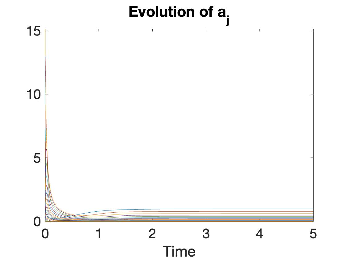
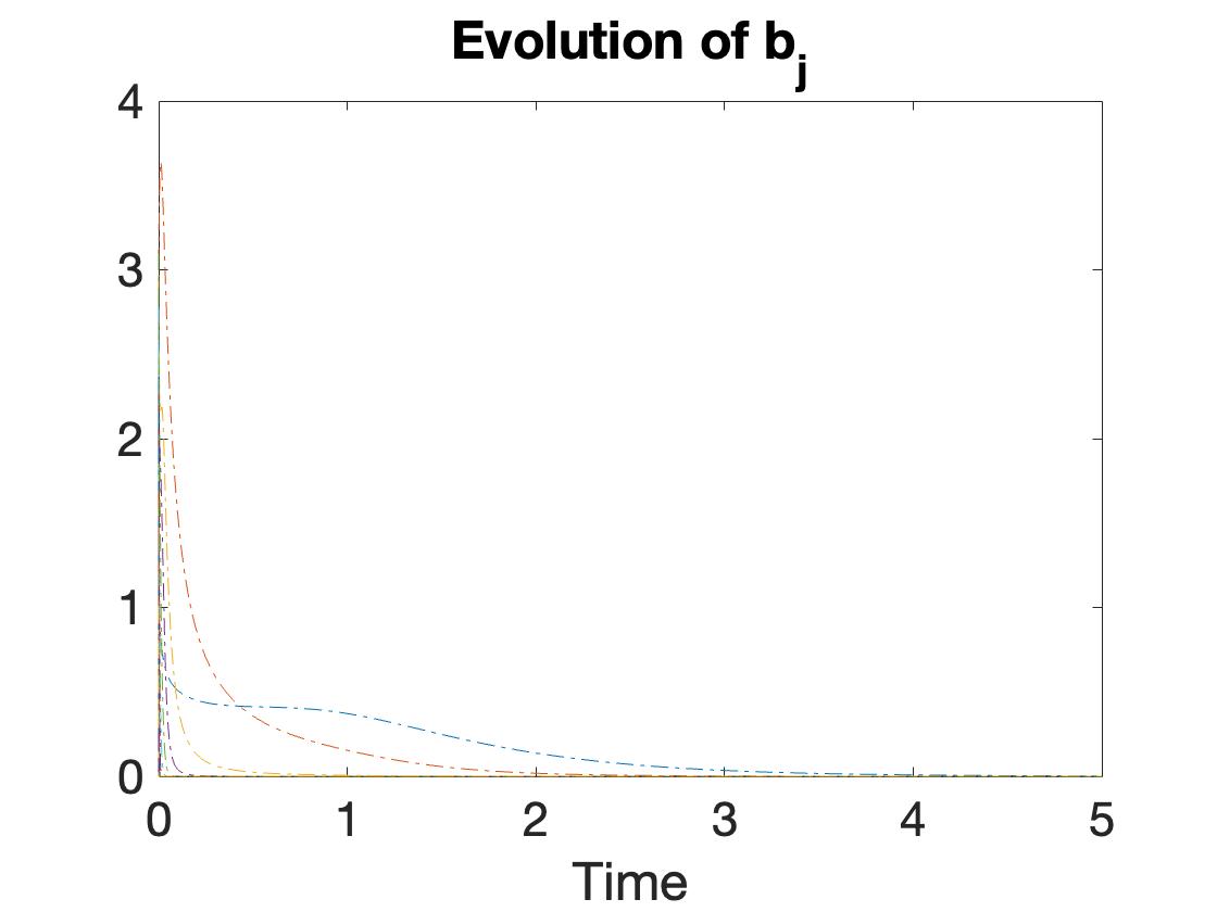
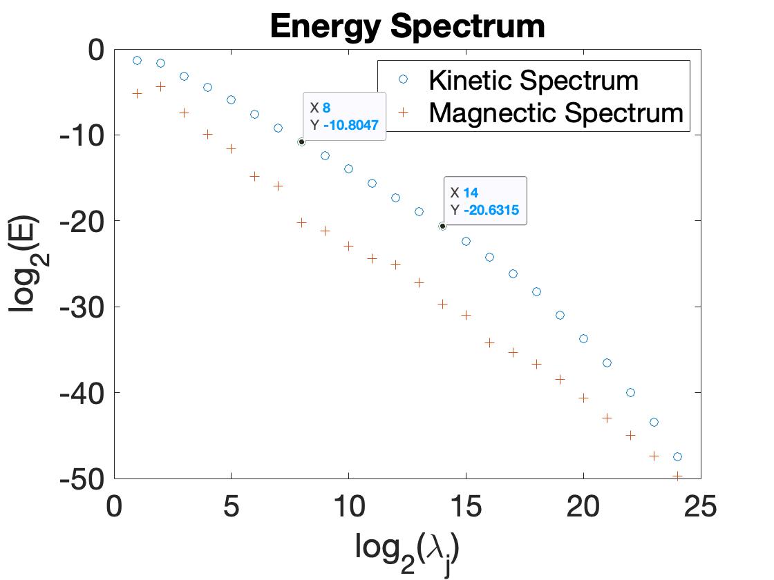
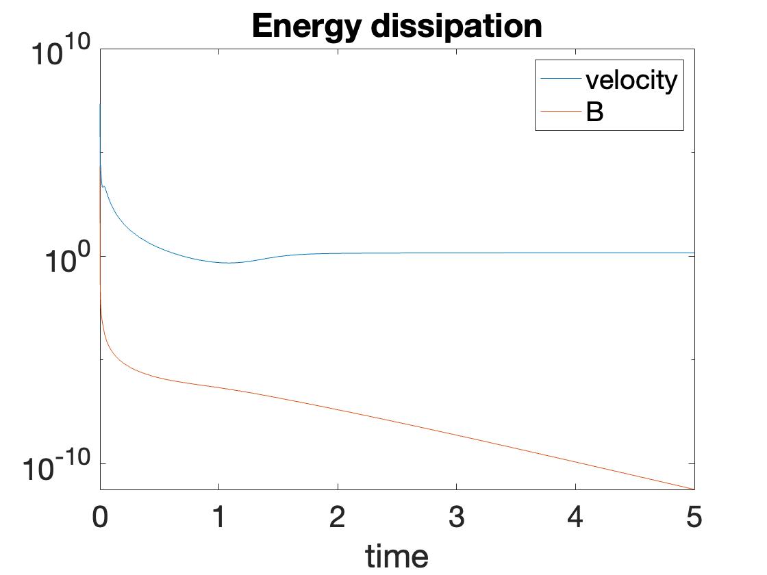
Figure 1. Forward cascade with $\theta=1$.

8.1. Model with forward energy cascade

For (1.3), we consider the following cutoff system:

$$\begin{split}a^{\prime}_{0}=&-\nu\lambda_{0}^{2}a_{0}-\lambda_{0}^{\theta}a_{0}a_{1}-\lambda_{0}^{\theta}b_{0}b_{1}+f_{0},\\ b^{\prime}_{0}=&-\mu\lambda_{0}^{2}b_{0}+\lambda_{0}^{\theta}a_{0}b_{1}-\lambda_{0}^{\theta}b_{0}a_{1},\\ a^{\prime}_{j}=&-\nu\lambda_{j}^{2}a_{j}-\left(\lambda_{j}^{\theta}a_{j}a_{j+1}-\lambda_{j-1}^{\theta}a_{j-1}^{2}\right)-\left(\lambda_{j}^{\theta}b_{j}b_{j+1}-\lambda_{j-1}^{\theta}b_{j-1}^{2}\right),\ \ 1\leq j\leq N-1,\\ b^{\prime}_{j}=&-\mu\lambda_{j}^{2}b_{j}+\lambda_{j}^{\theta}a_{j}b_{j+1}-\lambda_{j}^{\theta}b_{j}a_{j+1},\ \ 1\leq j\leq N-1,\\ a^{\prime}_{N}=&-\nu\lambda_{N}^{2}a_{N}-\left(\lambda_{N}^{\theta}a_{N}a_{N+1}-\lambda_{N-1}^{\theta}a_{N-1}^{2}\right)-\left(\lambda_{N}^{\theta}b_{N}b_{N+1}-\lambda_{N-1}^{\theta}b_{N-1}^{2}\right),\\ b^{\prime}_{N}=&-\mu\lambda_{N}^{2}b_{N}+\lambda_{N}^{\theta}a_{N}b_{N+1}-\lambda_{N}^{\theta}b_{N}a_{N+1}.\\ \end{split}$$ (8.39)

In the case of inviscid non-resistive dyadic MHD (1.3), i.e $\nu=\mu=0$, Lemma 3.4 indicates that we have steady states $(\bar{a},\bar{b})$ satisfying $\bar{a}_{j}=\lambda^{\frac{1}{6}\theta}f_{0}^{\frac{1}{2}}A_{0}\lambda_{j}^{-\frac{1}{3}\theta}$ and $\bar{b}_{j}=\lambda^{\frac{1}{6}\theta}f_{0}^{\frac{1}{2}}B_{0}\lambda_{j}^{-\frac{1}{3}\theta}$ with $A_{0}^{2}+B_{0}^{2}=1$. In numerical simulation, we can take

$$a_{N+1}=\bar{a}_{N+1}=\lambda^{\frac{1}{6}}f_{0}^{\frac{1}{2}}A_{0}\lambda_{N+1}^{-\frac{1}{3}\theta},\ \ b_{N+1}=\bar{b}_{N+1}=\lambda^{\frac{1}{6}}f_{0}^{\frac{1}{2}}B_{0}\lambda_{N+1}^{-\frac{1}{3}\theta},$$

as an approximation for sufficiently small $\nu$ and $\mu$. Therefore, we set $\nu=5\cdot 10^{-7}$ and $\mu=10^{-7}$. Fix $\lambda=2$. Other parameters are chosen as

$$\theta=1,\ \ f_{0}=1.5,\ \ N=24,\ \ A_{0}=\frac{1}{2},\ \ B_{0}=\frac{\sqrt{3}}{2}.$$

Regarding initial data, we choose random data for $a_{j}(0)$ on $[0,15]$ and for $b_{j}(0)$ on $[0,4]$. Under this setting, the results of one numerical run are shown in Figure 1. The time evolution of $a_{j}$ and $b_{j}$ with $0\leq j\leq N$ are illustrated in Figure 1 (a) and (b), respectively. We observe that solutions $a_{j}$ converge to a steady state at large time and solutions remain positive; while solutions $b_{j}$ remain non-negative and converge to 0. Figure 1 (c) shows the kinetic and magnetic energy spectrum. One can see that between mode 3 and mode 18, the kinetic spectrum lies on a straight line with slop $\sim\frac{-20.6315+10.8047}{14-8}\sim-\frac{5}{3}$. We note that when $\theta=1$ and hence $\delta=3$, the predicted kinetic energy spectrum in Section 4 has the scaling $\mathcal{E}_{u}(k)\sim k^{\frac{\delta-8}{3}}=k^{-\frac{5}{3}}$ in the inertial range. Therefore the numerical result justifies the scaling law. Moreover, we note in Figure 1 (c) that after mode 18, the spectrum becomes steeper, which is supposed to be the dissipation range. In fact, in view of the scaling analysis of Section 4, the critical dissipation wavenumber that separates the dissipation range from the inertial range has the scaling

$$\kappa_{\mathrm{d}}^{u}\sim(\nu^{-3}\varepsilon_{u})^{\frac{1}{\delta+1}}=(\nu^{-3}\bar{a}_{0}f_{0})^{\frac{1}{\delta+1}}\sim 17$$

under the choice of the parameters. Thus, the numerical simulation is in agreement with the scaling law. Regarding the magnetic energy spectrum, it is more or less on a line with similar slop to that of the kinetic energy spectrum with some discrepancy. Figure 1 (d) shows the kinetic and magnetic energy dissipation: $\nu\sum_{j=0}^{N}\lambda_{j}^{2}a_{j}^{2}(t)$ and $\mu\sum_{j=0}^{N}\lambda_{j}^{2}b_{j}^{2}(t)$. Notice that kinetic energy dissipation converges to a non-zero constant and the magnetic energy dissipation converges to zero, which shows consistence with the results of Figure 1 (a) and (b).

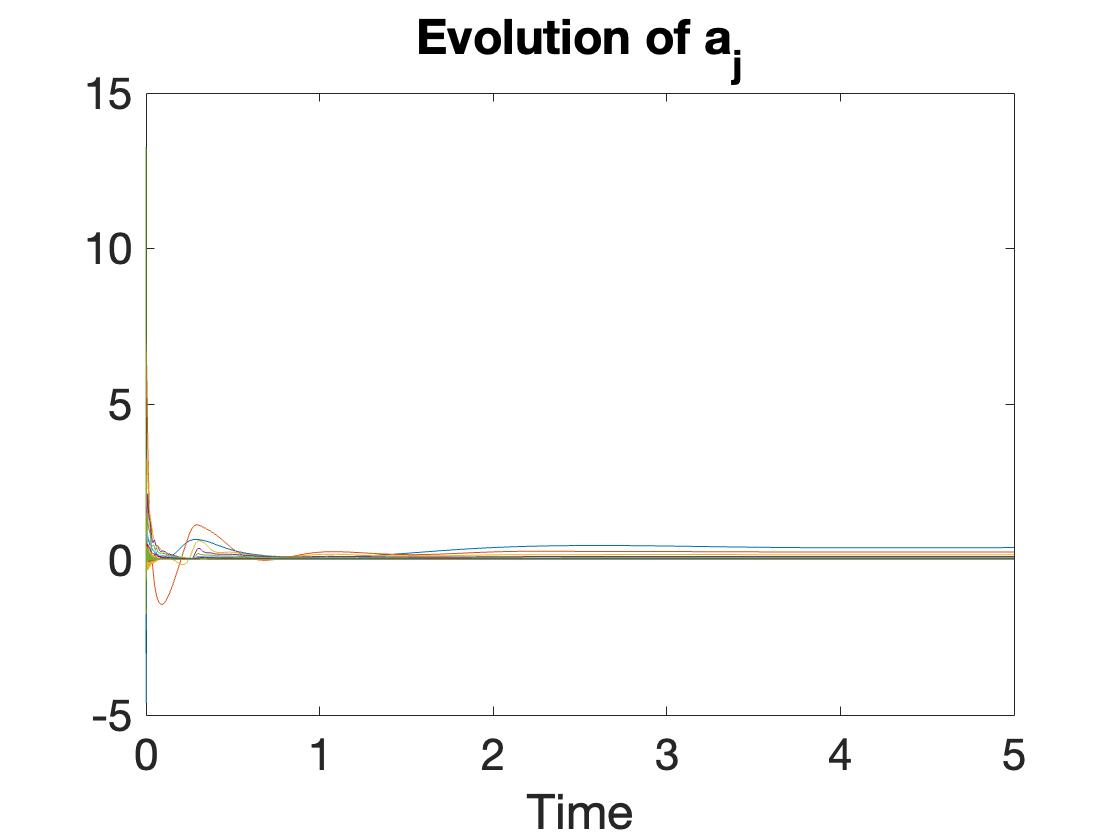
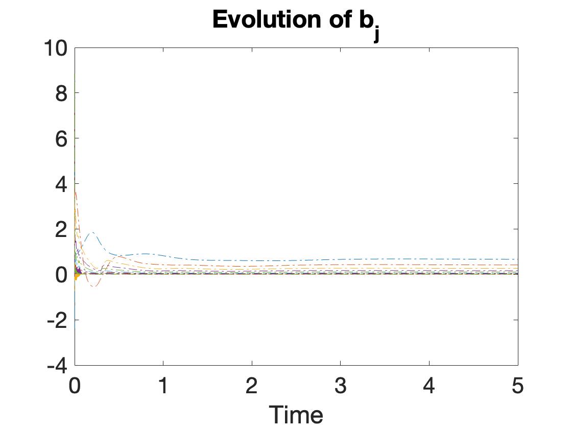
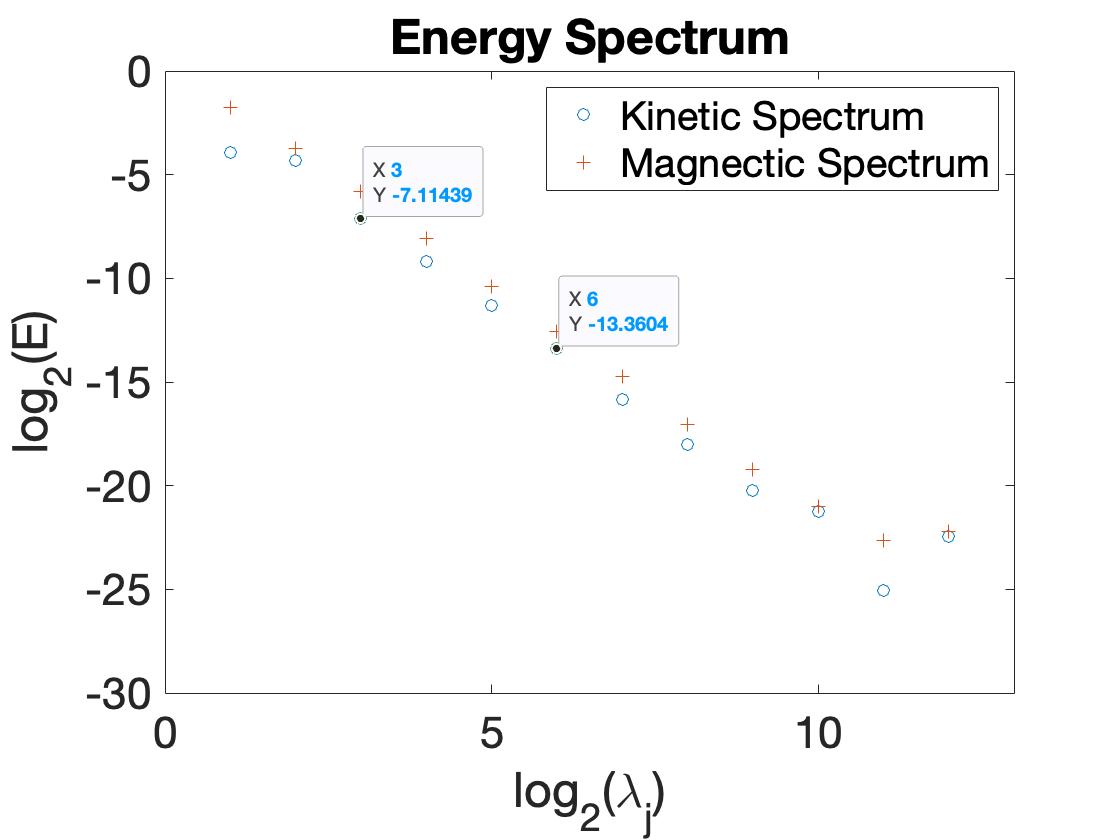
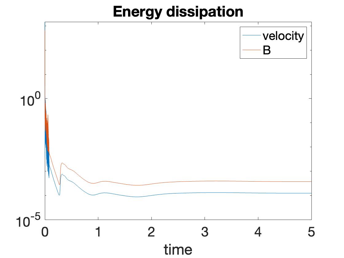
Figure 2. Forward cascade with $\theta=2$.

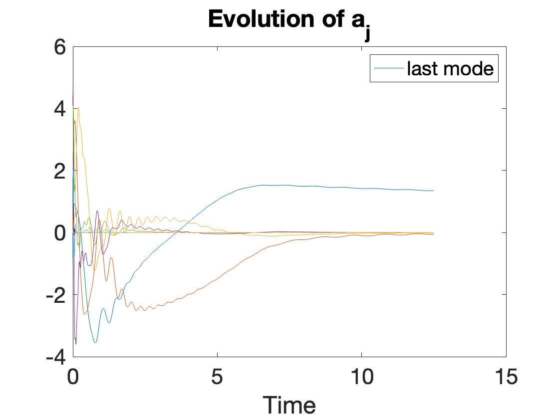
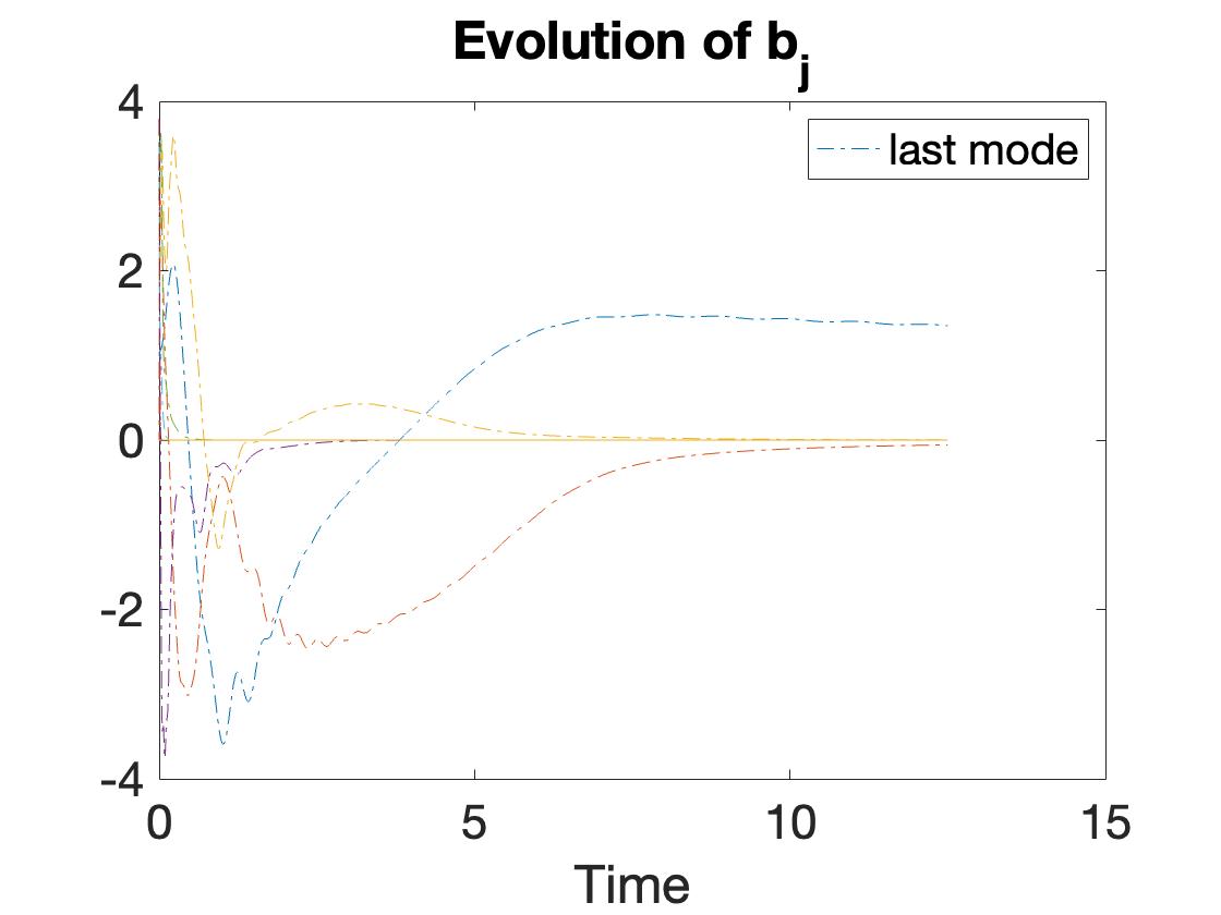
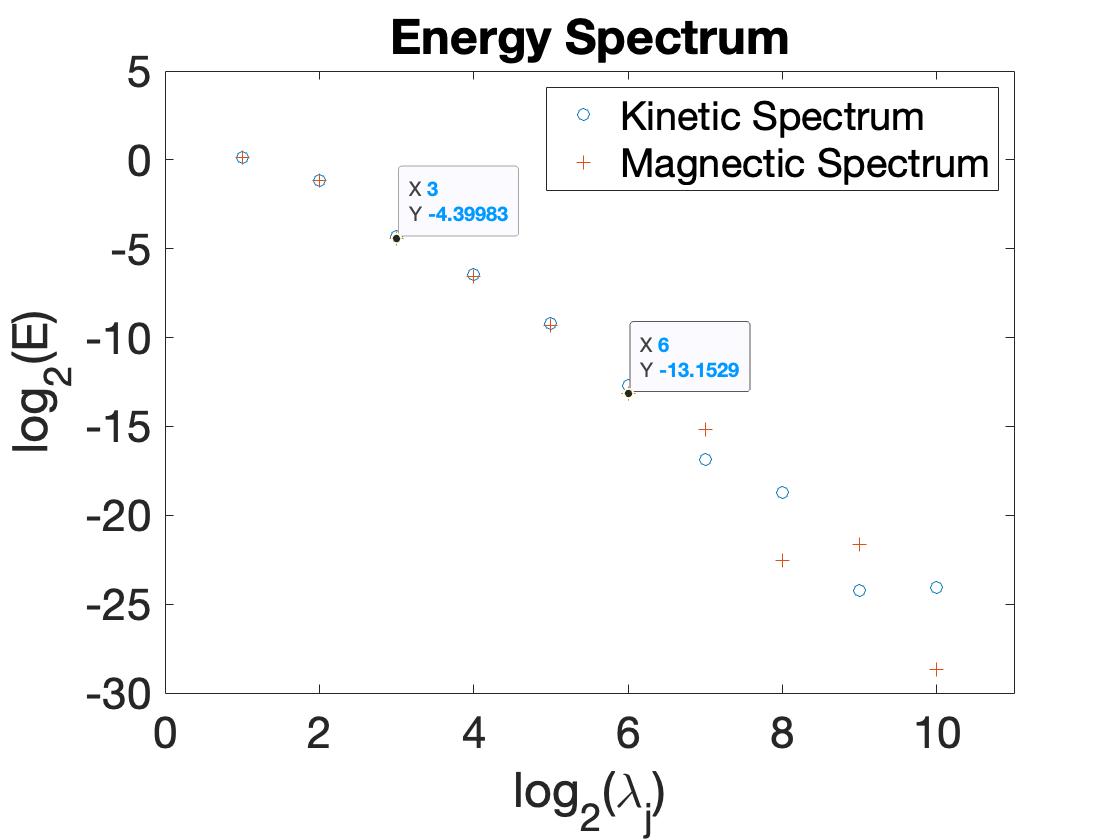
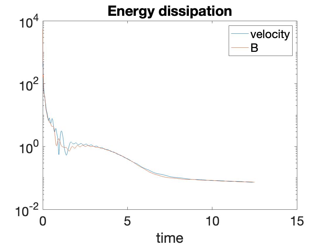
Figure 3. Forward and backward cascades with $\theta=1$.

In the second setting, we take $\theta=2$ ($\delta=1$) and $N=12$, and all the other parameters remain unchanged. In this case, the intermittency dimension is smaller and the nonlinearity is stronger. The numerical simulation is shown in Figure 2. From Figure 2 (a) and (b), we observe that solutions starting from positive initial data can become negative; however, the solutions eventually converge to a positive steady state. We also note the solutions $b_{j}$ converge to non-zero constants. Again, the energy dissipation of Figure 2 (d) shows consistence with Figure 2 (a) and (b). Comparing Figure 2 (a), (b) and (d) and Figure 1 (a), (b) and (d), it is not hard to see that the enhanced nonlinearity influences the behaviors of the solution. The energy spectrum shown in Figure 1 (c) confirms the scaling law

$$\mathcal{E}_{u}(k)\sim k^{\frac{\delta-8}{3}}=k^{-\frac{7}{3}},\ \ \mbox{with}\ \ \delta=1.$$

8.2. Model with both forward and backward energy cascades

For system (1.4), we consider the following cutoff approximating system:

$$\begin{split}a^{\prime}_{0}=&-\nu\lambda_{0}^{2}a_{0}-\lambda_{0}^{\theta}a_{0}a_{1}+\lambda_{0}^{\theta}b_{0}b_{1}+f_{0},\\ b^{\prime}_{0}=&-\mu\lambda_{0}^{2}b_{0}-\left(\lambda_{0}^{\theta}a_{0}b_{1}-\lambda_{0}^{\theta}b_{0}a_{1}\right),\\ a^{\prime}_{j}=&-\nu\lambda_{j}^{2}a_{j}-\left(\lambda_{j}^{\theta}a_{j}a_{j+1}-\lambda_{j-1}^{\theta}a_{j-1}^{2}\right)+\left(\lambda_{j}^{\theta}b_{j}b_{j+1}-\lambda_{j-1}^{\theta}b_{j-1}^{2}\right),\ \ 1\leq j\leq N-1,\\ b^{\prime}_{j}=&-\mu\lambda_{j}^{2}b_{j}-\left(\lambda_{j}^{\theta}a_{j}b_{j+1}-\lambda_{j}^{\theta}b_{j}a_{j+1}\right),\ \ 1\leq j\leq N-1,\\ a^{\prime}_{N}=&-\nu\lambda_{N}^{2}a_{N}-\left(\lambda_{N}^{\theta}a_{N}a_{N+1}-\lambda_{N-1}^{\theta}a_{N-1}^{2}\right)+\left(\lambda_{N}^{\theta}b_{N}b_{N+1}-\lambda_{N-1}^{\theta}b_{N-1}^{2}\right),\\ b^{\prime}_{N}=&-\mu\lambda_{N}^{2}b_{N}-\left(\lambda_{N}^{\theta}a_{N}b_{N+1}-\lambda_{N}^{\theta}b_{N}a_{N+1}\right).\\ \end{split}$$ (8.40)

By Lemma 7.2, we know that the dyadic model (1.4) with $\mu=\nu=0$ has steady state $(\bar{a},\bar{b})$ satisfying

$$\bar{a}_{j}=\lambda^{\frac{1}{6}\theta}f_{0}^{\frac{1}{2}}A_{0}\lambda_{j}^{-\frac{1}{3}\theta},\ \ \bar{b}_{j}=\lambda^{\frac{1}{6}\theta}f_{0}^{\frac{1}{2}}B_{0}\lambda_{j}^{-\frac{1}{3}\theta}$$

with $A_{0}^{2}-B_{0}^{2}=1$. In numerical simulation with small $\nu$ and $\mu$, as an approximation, we choose

$$a_{N+1}=\bar{a}_{N+1}=\lambda^{\frac{1}{6}}f_{0}^{\frac{1}{2}}A_{0}\lambda_{N+1}^{-\frac{1}{3}\theta},\ \ b_{N+1}=\bar{b}_{N+1}=\lambda^{\frac{1}{6}}f_{0}^{\frac{1}{2}}B_{0}\lambda_{N+1}^{-\frac{1}{3}\theta}.$$

Numerical experiments indicate that this model is more sensitive to the choice of the force $f_{0}$, viscosity $\nu$ and resistivity $\mu$. For the same size force $f_{0}$, $\nu$ and $\mu$ as for the approximating model (8.39), solutions grow more rapidly. Moreover, the model seems very sensitive to the choice of initial data as well. With the same parameters, solutions for some random data grows more rapidly than other solutions. Based on these observations, we choose relatively large $\nu=\mu=0.01$ and small force $f_{0}=0.05$, and

$$\theta=1,\ \ N=10,\ \ A_{0}=\sqrt{2},\ \ B_{0}=1.$$

We choose random data for $a_{j}(0)$ on $[0,5]$ and for $b_{j}(0)$ on $[0,4]$. The numerical results are shown in Figure 3. The evolution of solutions $a_{j}$ and $b_{j}$ in Figure 3 (a) and (b) shows that solutions do not remain positive even though the initial data is positive. In contrast to Figure 1 (a) and (b), it takes much longer time for the solutions of (8.40) to converge. We point out that the last modes $a_{N}$ and $b_{N}$ are far apart from other modes after convergence to a steady state; this could be an artifact due to the choice of $a_{N+1}$ and $b_{N+1}$. The energy dissipation shown in Figure 3 (d) is also consistent with Figure 3 (a) and (b). It is interesting to notice that the energy spectrum shown in Figure 3 (c) exhibits a scaling law; however, the slop is close to $-\frac{8.75}{3}$ which has a big discrepancy with the predicted slop $-\frac{5}{3}$. Many numerical runs with the same parameters show such discrepancy. Further investigation for the model with forward and backward energy cascades will be addressed in future work.

References

• [1] D. Barbato, F. Morandin, and M. Romito. Smooth solutions for the dyadic model. Nonlinearity, 24 (11): 3083–3097, 2011.
• [2] L. Biferale. Shell models of energy cascade in turbulence. Annu. Rev. Fluid Mech., 35: 441468, 2003.
• [3] D. Biskamp. Cascade models for magnetohydrodynamic turbulence. Phys. Rev. E50: 2702–2711, 1994.
• [4] A. Cheskidov. Blow-up in finite time for the dyadic model of the Navier-Stokes equations . Trans. Amer. Math. Soc., 360 (10): 5101-5120, 2008.
• [5] A. Cheskidov and M. Dai. Kolmogorov’s dissipation number and the number of degrees of freedom for the 3D Navier-Stokes equations. Proceedings of the Royal Society of Edinburg, Section A, Vol. 149, Issue 2: 429–446, 2019.
• [6] A. Cheskidov, M. Dai and L. Kavlie. Determining modes for the 3D Navier-Stokes equations. Physica D: Nonlinear Phenomena, Vol. 374-375: 1–9, 2018.
• [7] A. Cheskidov and S. Friedlander. The vanishing viscosity limit for a dyadic model. Physica D, 238:783–787, 2009.
• [8] P. Constantin, B. Levant, and E.Titi. Analytic study of the shell model of turbulence. Physica D: Nonlinear Phenomena, 219 (2): 120–141, 2006.
• [9] M. Dai. Blow-up of dyadic MHD models with forward energy cascade. arXiv: 2102.03498, 2021.
• [10] M. Dai. Dyadic models with intermittency dependence for the Hall MHD. arXiv: 2006.15094, 2020.
• [11] M. Dai and S. Friedlander. Uniqueness and non-uniqueness results for dyadic MHD models. arXiv: 2107.04073, 2021.
• [12] E. I. Dinaburg and Y. G. Sinai. A quasi-linear approximation of three-dimensional Navier-Stokes system. Moscow Math. J., 1: 381–388, 2001.
• [13] N. Filonov. Uniqueness of the Leray-Hopf solution for a dyadic model. Transactions of the American Mathematical Society, Vol. 369 (12): 8663–8684, 2017.
• [14] N. Filonov and P. Khodunov. Non-uniqueness of Leray-Hopf solutions for a dyadic model. arXiv: 2004.01074, 2020.
• [15] U. Frisch. Turbulence: The Legacy of A. N. Kolmogrov. Cambridge University Press, Cambridge, 1995.
• [16] E. B. Gledzer. System of hydrodynamic type admitting two quadratic integrals of motion. Soviet Phys. Dokl., 18: 216-217, 1973.
• [17] C. Gloaguen, J. Léorat, A. Pouquet and R. Grappin. A scalar model for MHD turbulence. Physica D.: Nonlinear Phenomena, 17(2):154–182, 1985.
• [18] A. Kolmogoroff. The local structure of turbulence in incompressible viscous fluid for very large Reynold’s numbers. C. R. (Doklady) Acad. Sci. URSS (N.S.), 30:301–305, 1941.
• [19] V. S. L’vov, E. Podivilov, A. Pomyalov, I. Procaccia, and D. Vandembroucq. Improved shell model of turbulence. Phys. Rev. E (3) 58: 1811–1822, 1998.
• [20] A. M. Obukhov. Some general properties of equations describing the dynamics of the atmosphere. Izv. Akad. Nauk SSSR Ser. Fiz. Atmosfer. i Okeana, 7:695–704, 1971.
• [21] K. Ohkitani and M. Yamada. Temporal intermittency in the energy cascade process and local Lyapunov analysis in fully-developed model of turbulence. Progr. Theoret. Phys., 81: 329–341, 1989.
• [22] F. Plunian, R. Stepanov and P. Frick. Shell models of magnetohydrodynamic turbulence. Physics Reports, vol. 523, 2013.