OPRE-2021-08-497.R1

Tight Guarantees for Static Threshold Policies in the Prophet Secretary Problem

Nick Arnosti Department of Industrial and Systems Engineering, University of Minnesota, Minneapolis, MN, arnosti@umn.edu Will Ma Graduate School of Business, Columbia University, New York, NY 10027, wm2428@gsb.columbia.edu

In the prophet secretary problem, $n$ values are drawn independently from known distributions, and presented in a uniformly random order. A decision-maker must accept or reject each value when it is presented, and may accept at most $k$ values in total. The objective is to maximize the expected sum of accepted values.

We analyze the performance of static threshold policies, which accept the first $k$ values exceeding a fixed threshold (or all such values, if fewer than $k$ exist). We show that an appropriate threshold guarantees $\gamma_{k}=1-e^{-k}k^{k}/k!$ times the value of the offline optimal solution. Note that $\gamma_{1}=1-1/e$, and by Stirling’s approximation $\gamma_{k}\approx 1-1/\sqrt{2\pi k}$. This represents the best-known guarantee for the prophet secretary problem for all $k>1$, and is tight for all $k$ for the class of static threshold policies.

We provide two simple methods for setting the threshold. Our first method sets a threshold such that $k\cdot\gamma_{k}$ values are accepted in expectation, and offers an optimal guarantee for all $k$. Our second sets a threshold such that the expected number of values exceeding the threshold is equal to $k$. This approach gives an optimal guarantee if $k>4$, but gives sub-optimal guarantees for $k\leq 4$. Our proofs use a new result for optimizing sums of independent Bernoulli random variables, which extends a classical result of Hoeffding (1956) and is likely to be of independent interest. Finally, we note that our methods for setting thresholds can be implemented under limited information about agents’ values.

This version from June 7th, 2022. Full version of EC2022 paper.

1 Introduction

A decision-maker is endowed with $k$ identical, indivisible items to allocate among $n>k$ applicants who arrive sequentially. Each applicant $i=1,\ldots,n$ has a value $V_{i}\geq 0$ for receiving an item. Upon the arrival of applicant $i$, the decision-maker observes $V_{i}$ and must either immediately “accept” and allocate an item to applicant $i$, or irrevocably “reject” applicant $i$ (which is the only option if no items remain). The policymaker wishes to maximize the sum of the values of accepted applicants.

The Prophet Secretary problem. This style of sequential accept/reject problem has been studied under different assumptions about the decision-maker’s initial information and the order in which applicants arrive. In the secretary problem, the decision-maker knows nothing about applicants’ values, but applicants arrive in a uniformly random order. Meanwhile, papers on prophet inequalities typically assume that each value $V_{i}$ is drawn independently from a known distribution $F_{i}$. This paper studies the prophet secretary problem introduced by Esfandiari et al. (2017), in which values are drawn independently from known distributions and applicants arrive in a uniformly random order. We discuss the background behind these naming conventions in Section 2.1.

Static Threshold Policies. We focus especially on static threshold policies, which fix a real number $t$, and accept the first $k$ applicants whose value exceeds $t$. These policies are simple to explain and implement, and are non-discriminatory, in that they use the same threshold for every applicant (so long as items remain). Perhaps for these reasons, static threshold policies arise frequently in practice. They are typically implemented by combining eligibility criteria with first-come-first-served allocation. For example, policymakers often use an income ceiling to determine eligibility for subsidized housing, and then award this housing using a first-come-first-served waitlist. Similarly, many popular marathons set “qualifying times”, and allow qualified runners to claim race slots until all slots have been taken.

Static threshold policies have also been widely deployed is the allocation of COVID-19 vaccines. In early 2021, many state governments sorted people into priority tiers. At any given time, only the highest-priority tiers were eligible for vaccination. However, eligible individuals could claim appointments on a first-come-first-served basis. When determining the eligibility threshold, policymakers balanced two risks. Using very strict criteria could result in unclaimed appointments and discarded doses. Expanding eligibility could result in appointments being claimed as soon as they became available, causing some high-priority individuals to be turned away.

Key questions and contributions. Experiences like this one inspire two natural questions. First, what is the cost of using eligibility criteria alongside first-come-first-served allocation, rather than waiting for all applicants to arrive and then selecting those with the highest priority? Second, how should the eligibility threshold be set to balance the two risks described above? We use the prophet secretary model to investigate both questions.

Our first contribution is to exactly characterize the worst-case performance of static threshold policies. More specifically, we show that there always exists a static threshold policy whose performance is at least a $(1-e^{-k}\frac{k^{k}}{k!})$-fraction of the full-information benchmark. We also provide an example showing that no better guarantee is possible.

Our second contribution is to show that simple and intuitive algorithms for setting the eligibility threshold achieve optimal guarantees. Our first algorithm sets a threshold based on the expected number of allocated items, while the second is based on the expected number of eligible applicants. In Section 5, we note that these algorithms can also be deployed in settings where values are only imperfectly observed, and explain why this is relevant for the allocation of COVID-19 vaccines.

Despite their simplicity, our algorithms not only provide optimal guarantees within the class of static threshold policies, but also provide the best-known guarantees for any online policy that observes one applicant’s value at a time and must make an irrevocable decision for each applicant before moving on to the next.

Terminology and notation. Before presenting our results, we define a few concepts. An instance of the prophet secretary problem is given by the number of items $k$ and the number of applicants $n$, along with $n$ cumulative distribution functions ${\bf F}=(F_{1},\ldots,F_{n})$ on the non-negative real numbers. The values $V_{i}$ are drawn independently from distributions $F_{i}$, and arrive in a uniformly random order. If $F_{i}=F_{j}$ for all $i,j$, we say that values are independently and identically distributed (IID).

Given values $\{V_{i}\}_{i=1}^{n}$, demand at a threshold $t$ is the number of values that exceed $t$. The number of accepted applicants is equal to the minimum of demand and the supply $k$. Utilization is the fraction of the supply that is allocated, and is calculated by dividing the number of accepted applicants by $k$. When using a static threshold policy with threshold $t$, the performance of $t$ is the expected sum of accepted applicants’ values. We compare this performance to the expected sum of the $k$ highest values, which we call the prophet’s value. More formal definitions for all of these concepts are provided in Definition 3.1 in Section 3. Finally, for $k\geq 1$, define the constant

$$\gamma_{k}:=1-e^{-k}\frac{k^{k}}{k!}.$$ (1)

1.1 An Upper Bound for Static Threshold Policies

We first derive an upper bound on the performance for any static threshold policy.

Theorem 1.1

For any $k\geq 1$ and $\epsilon>0$, there exists an instance $(k,{\bf F})$ with IID values such that the performance of any threshold is less than $\gamma_{k}+\epsilon$ times the prophet’s value.

This upper bound is for static threshold policies, and no longer holds if more general policies are allowed. For example, when $k=1$ we have $\gamma_{1}=1-1/e\approx 0.632$, but there exist policies that achieve a guarantee of 0.669 (Correa et al. 2020), and 0.745 if values are IID (Correa et al. 2017).

Our proof of Theorem 1.1 consists of a careful analysis of the following example.

Example 1.2

Let the values $V_{i}$ be independent and identically distributed according to

$$\SingleSpacedXI V_{i}=\begin{cases}nW_{k}&w.p.~{}1/n^{2}\\ 1&w.p.~{}1-1/n^{2},\\ \end{cases}\DoubleSpacedXI$$

where $W_{k}=k\frac{\mathbb{P}(\mathrm{Pois}(k)<k)}{\mathbb{P}(\mathrm{Pois}(k)>k)}$, and $\mathrm{Pois}(k)$ denotes a Poisson random variable with mean $k$.

On this example, the prophet always accepts $k$ values, and takes high values whenever they occur. The prophet’s value is close to $k+W_{k}$. When setting a static threshold, the key question is whether to accept applicants with $V_{i}=1$. Always accepting these applicants results in performance close to $k$, while rejecting them results in performance close to $W_{k}$. We show that even accepting these applicants with some probability $p\in(0,1)$ cannot perform better than $\gamma_{k}(k+W_{k})$.

1.2 A Matching Lower Bound

Example 1.2 gives an upper bound for the performance of static threshold policies. We now show that this bound can be attained by setting the threshold so that expected utilization equals $\gamma_{k}$.

Theorem 1.3

For any instance $(k,{\bf F})$, the performance of any threshold such that expected utilization is equal to $k$ is at least $\gamma_{k}$ times the prophet’s value.

Remark 1.4

If each distribution $F_{i}$ is continuous, then expected utilization decreases continuously from 1 (at $t=0$) to $0$ (as $t\rightarrow\infty$), so it is always possible to choose a threshold such that expected utilization equals $\gamma_{k}$. In the case of discontinuous (discrete) distributions, tie-breaking may be required. In this case, we consider policies defined by a threshold $t\geq 0$ and a tie-break probability $p\in[0,1]$. If $V_{i}$ is exactly equal to $t$ and items remain when $i$ is considered, then the policy $(t,p)$ accepts item $i$ with probability $p$ (independently from all other randomness). Tie-breaking makes it possible to adjust expected utilization (and expected demand) continuously, and is a standard way to handle discrete distributions. For example, it is also used in Ehsani et al. (2018) and Chawla et al. (2020). All of our results apply to any static threshold policy with tie-breaking.

For any $k>1$, Theorem 1.3 implies the best-known guarantees (relative to the prophet’s value) for any online policy in the prophet secretary problem. In fact, our proof establishes that the statement remains true if the prophet’s value is replaced by a stronger benchmark (sometimes called the “LP relaxation”, “fluid limit”, or “ex ante relaxation”) that is constrained to accept at most $k$ values in expectation, rather than on each realization. We formally define this benchmark in Section 3. It is well-known that no online policy can guarantee performance better than $\gamma_{k}$ times the value of the LP relaxation (see e.g. Yan 2011), so Theorem 1.3 also implies that static threshold policies achieve optimal guarantees against this benchmark.

It is insightful to compare $\gamma_{k}$ to guarantees from prior work. Figure 1 plots our guarantee against one proven by Cominetti et al. (2010), as well as a guarantee of Chawla et al. (2020) for the case where values arrive in an order selected by an adversary. In this latter model, it is known that no static threshold policy can achieve performance better than $1-\Theta(\sqrt{\log k/k})$ times the prophet’s value. By contrast, Stirling’s approximation implies that $\gamma_{k}\approx 1-1/\sqrt{2\pi k}$, so there is a separation of order $\sqrt{\log k}$ in the asymptotic loss between models with random and adversarial arrival order.

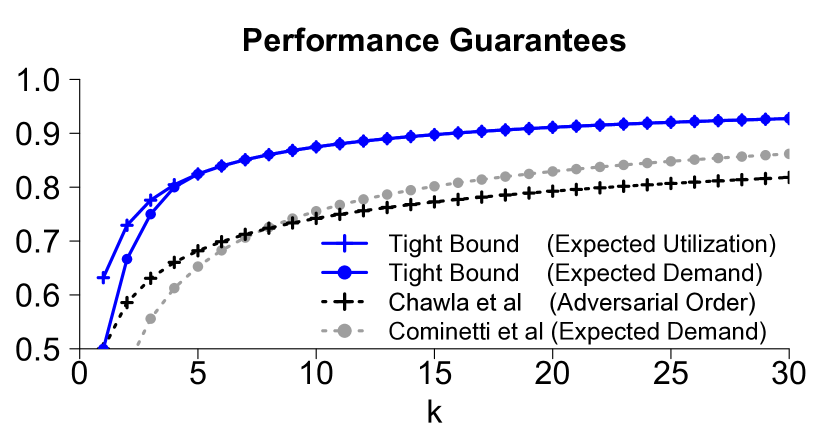
Figure 1: Our tight bounds compared to bounds from prior work. Chawla et al. (2020) give lower bounds on the performance of static threshold policies when the arrival order is selected by an adversary. These bounds carry over to our setting, where the arrival order is random. In this setting, our Theorem 1.3 establishes that a policy based on expected utilization gives the best-possible guarantee. In the random arrival model, Cominetti et al. (2010) provide lower bounds on the performance of a policy that sets expected demand equal to $k$. Our Theorem 1.6 improves their result by giving a tight guarantee for this policy.

1.3 Thresholds Based on Expected Demand

Jointly, Theorems 1.1 and 1.3 identify, for each $k$, the exact guarantee $\gamma_{k}$ that can be achieved by static threshold policies. However, it is natural to wonder about other ways to set the threshold. Do other simple policies also achieve this same guarantee?

One advantage of our analysis is that it only requires small modifications to answer this question. We focus on a simple policy which sets the threshold so that the expected number of values exceeding the threshold is equal to $k$. This policy is intuitive, and has previously been studied by Cominetti et al. (2010), who show (under an assumption on the distributions $F_{i}$) that its performance is at least $1-\sqrt{\frac{1+1/\sqrt{k}}{2(k+1)}}$ times the prophet’s value. Theorem 1.6 gives tight bounds for the performance of this policy which hold for any value distributions. Figure 1 offers a visual comparison between our tight bounds and those of Cominetti et al. (2010).

It is intuitive that if expected demand is equal to $k$ and $k$ is large, then realized demand should be “close” to $k$, implying near-optimal performance. By contrast, when $k$ is small, the following example shows that setting expected demand equal to $k$ does not guarantee strong performance.

Example 1.5

Fix $k$ and consider a small $\varepsilon>0$. Let there be $n=k+1$ applicants. Applicants $i=1,\ldots,k$ all have a value that is distributed as: 1 with probability $1-\varepsilon/k$; 0 otherwise. The value of applicant $k+1$ is distributed as: $1/\varepsilon^{2}$ with probability $\varepsilon$; 0 otherwise.

On this example, the prophet’s value is at least $1/\varepsilon$, as this is the expected value of applicant $k+1$. Meanwhile, the policy that sets expected demand equal to $k$ will accept all applicants with non-zero values. Therefore, if applicants $1,\ldots,k$ all have value $1$ and also arrive before applicant $k+1$, then the final applicant is rejected. By a union bound, the probability of this is at least $\frac{1-\varepsilon}{k+1}$. Because the contribution from the first $k$ applicants is upper-bounded by $k$, the value of this policy is at most

$$\frac{1}{\varepsilon^{2}}\cdot\varepsilon(1-\frac{1-\varepsilon}{k+1})+k=\frac{1}{\varepsilon}\cdot\frac{k}{k+1}+\frac{1}{k+1}+k.$$

Taking $\varepsilon\to 0$, this shows that the policy which sets expected demand equal to $k$ does not guarantee more than $\frac{k}{k+1}$ times the prophet’s value.

Examples 1.2 and 1.5 both provide upper-bounds on the performance of a threshold set so that expected demand equals $k$. These upper bounds are $\gamma_{k}$ and $k/(k+1)$ times the prophet’s value, respectively. Our next result establishes that these examples represent worst cases for this policy.

Theorem 1.6

For any instance $(k,{\bf F})$, the performance of any threshold such that expected demand is equal to $k$ is at least $\min\{\gamma_{k},\frac{k}{k+1}\}$ times the prophet’s value.

Note that $\min\{\gamma_{k},\frac{k}{k+1}\}$ is $\frac{k}{k+1}$ when $k\leq 4$, and $\gamma_{k}$ when $k>4$. Therefore, Theorems 1.1 and 1.6 jointly imply that the policy of setting expected demand equal to $k$ achieves the best-possible guarantee when $k>4$.

In Example 1.5, we intuitively want expected demand to be below $k$, in order to increase the probability of accepting the high-value applicant. In fact, Hajiaghayi et al. (2007) analyze a policy that sets expected demand equal to $k-\sqrt{2k\log k}$. Unfortunately, we show in Proposition 5.1 that when $k\leq 4$, any algorithm that sets expected demand to some fixed target (even if that target is not $k$) cannot guarantee $\gamma_{k}$ times the prophet’s value. Thus, while expected utilization can be used to achieve optimal guarantees for all $k$, expected demand can only offer optimal guarantees for $k>4$. However, Proposition 5.2 establishes that if values are IID, then setting expected demand equal to $k$ offers a guarantee of $\gamma_{k}$ for all $k$. We present these results in Subsection 5.2.

1.4 A New Result for Bernoulli Optimization

Our analysis deploys a result about optimization problems involving sums of independent Bernoulli random variables. We highlight this result here, because we believe that it will be of general interest to researchers who encounter Bernoulli optimization problems in other contexts.

Given a vector of probabilities ${\bf p}\in[0,1]^{n}$, let $D_{\textbf{p}}$ denote the sum of independent Bernoulli random variables with means $p_{1},\ldots,p_{n}$. For any functions $f,g$ on the non-negative integers, consider the problem of choosing ${\bf p}$ to minimize $\operatorname*{\mathbb{E}}[f(D_{\textbf{p}})]$ subject to the constraint that $\operatorname*{\mathbb{E}}[g(D_{\textbf{p}})]=\phi$:

$$\Phi_{n}(f,g,\phi)=\min_{\textbf{p}\in[0,1]^{n}} \,\,\operatorname*{\mathbb{E}}[f(D_{\textbf{p}})]$$ (2)

s.t. $$\,\,\operatorname*{\mathbb{E}}[g(D_{\textbf{p}})]=\phi.$$

We show that for any functions $f$ and $g$, this problem has a solution with a very simple structure.

Theorem 1.7

For any $n\in\mathbb{N},$ any $f,g:\mathbb{N}_{0}\rightarrow\mathbb{R}$ and any $\phi\in\mathbb{R}$ such that (2) is feasible, there is a value $p\in(0,1)$ and an optimal solution p to (2) such that every $p_{i}\in\{0,p,1\}$.

This surprising result says that it suffices to consider cases where $D_{\textbf{p}}$ is equal to a constant plus a binomial random variable. Corollary 2.1 in Hoeffding (1956) establishes this result for arbitrary $f$ when $g$ is the identity, and Lemma 7 of Chawla et al. (2020) establishes this result when $f(d)=\min(1,d/k)$ and $g(d)=\mathbbm{1}(d<k)$. We believe that Theorem 1.7, which generalizes these preceding results, will be useful in settings beyond the prophet secretary problem.

1.5 Roadmap

Section 2 provides a thorough review of secretary problems and prophet inequalities, and compares our results to prior work. Section 3 provides formal definitions and proves Theorem 1.3. Section 4 provides the modifications necessary to prove Theorem 1.6. Section 5 discusses several extensions, including robustness of our policies when values are imperfectly observed, additional results for policies based on expected demand, and other rules for setting thresholds. We defer the proofs of Theorem 1.1 and Theorem 1.7, as well as all intermediate results, to the Appendix.

2 Literature Review

There is a large literature on sequential selection problems, dating back at least to Cayley (1875). The name “prophet secretary problem” was coined by Esfandiari et al. (2017), and inspired by prior work on “secretary problems” and “prophet inequalities”. Section 2.1 discusses the different modeling assumptions made by these two lines of work. Section 2.2 provides more detailed comparisons of existing results to our own.

2.1 Secretary Problems and Prophet Inequalities

The Secretary Problem. The most famous secretary problem features a sequence of $n$ unknown values arriving in uniformly random order, with the objective being to select the maximum. According to Ferguson (1989), this problem first appeared in print in a 1960 Scientific American column by Martin Gardner, but was widely known even before then. The optimal solution involves skipping the first $n/e$ values, and selecting the first value to exceed the highest of these (Dynkin 1963).

Prophet inequalities. Attributed to Krengel and Sucheston (1977, 1978), “prophet inequalities” commonly refer to comparisons between online and offline selection algorithms on a sequence of cardinal values drawn from known distributions. Samuel-Cahn (1984) initiated the study of static thresholds by proving the elegant result that setting a threshold equal to the median of the maximum value collects at least 1/2 of this maximum value in expectation. More recently, Kleinberg and Weinberg (2012) show that this same guarantee is achieved by setting a threshold equal to half of the expected maximum value.

Extensions of these problems. Many variants of these classic problems have been studied. In a single paper, (Gilbert and Mosteller 1966) consider four: one in which multiple items can be selected, another in which distributional information about the values is available up front, a third in which values arrive in an adversarial order, and a fourth in which the payoff is not $0$ or $1$ but rather depends on the values themselves. Meanwhile, follow-up work on prophet inequalities has studied the “free-order” setting where the decision-maker can choose the order of distributions (Hill 1983, Hill and Hordijk 1985, Beyhaghi et al. 2021, Agrawal et al. 2020) and also settings where the distribution of values is unknown but samples from these distributions are available (Azar et al. 2014, Correa et al. 2019a, Rubinstein et al. 2020).

Ferguson (1989) writes “Since there are so many variations of the basic secretary problem…it is worthwhile to try to define what a secretary problem is.” He concludes “a secretary problem is a sequential observation and selection problem in which the payoff depends on the observations only through their relative ranks and not otherwise on their actual values.”

However, many subsequent papers have followed a different convention, and used the term “secretary” to refer to problems where unknown values arrive in a uniformly random order. Rubinstein (2016) draws the following distinction:

In the Secretary Problem, the values of items are chosen adversarially, but their arrival order is random. In Prophet Inequality, the order is adversarial, but the values are drawn from known, independent but not identical distributions.

This terminology has been applied fairly consistently within the computer science literature. For example, Ezra et al. (2020) (“Secretary Matching with General Arrivals”) study matching models with adversarial values arriving in a random order, while Ezra et al. (2021) (“Prophet Matching with General Arrivals”) consider the case where values are drawn from known distributions and arrive in an order fixed by an adversary.

The “multiple-choice secretary” model of Kleinberg (2005) features $n$ adversarially selected values arriving in random order, as does later work on the knapsack (Babaioff et al. 2007a) and matroid (Babaioff et al. 2007b) secretary problems, secretary matching problem (Ezra et al. 2020), and secretary problem under general downward-closed feasibility constraints (Rubinstein 2016).

Similarly, prophet inequalities have been studied under $k$-unit (Hajiaghayi et al. 2007, Alaei 2014), matroid (Kleinberg and Weinberg 2012), knapsack (Dutting et al. 2020), matching (Ezra et al. 2021), and general downward-closed (Rubinstein 2016) feasibility constraints. All of these papers feature values drawn from known distributions, arriving in an order that may be selected by an adversary. This literature was surveyed by Hill and Kertz (1992), and more recent work is discussed in Lucier (2017), Correa et al. (2018).

Inspired by this convention, Esfandiari et al. (2017) use the phrase “prophet secretary problem” to describe settings in which values are drawn from (possibly heterogeneous) known distributions and presented in a uniformly random order. We adopt this terminology, while noting that it is not used universally. For example, Arlotto and Gurvich (2019) and Bray (2019) use the term “multisecretary” to refer to a problem where values are drawn IID from a known distribution. These papers study (additive) regret, in contrast to the multiplicative guarantees in our work.

2.2 Comparison to Existing Results

In this subsection we compare our guarantees to those in prior work. Kleinberg (2005) considers a “multiple-choice secretary” model in which $n$ values arrive in random order, and the decision-maker can accept $k$ values and wishes to maximize their sum. He provides an algorithm that guarantees $1-5/\sqrt{k}$ times the prophet’s value. Unlike his work, ours assumes that values are drawn independently from known distributions. This allows us to use simple static threshold policies, and to get a better guarantee of $\gamma_{k}\approx 1-1/\sqrt{2\pi k}$.

The remainder of this section compares to papers which assume that values are drawn from known distributions. Some of these papers assume values are IID; others assume they are drawn from heterogeneous distributions and arrive in a random order; others assume that the arrival order is chosen by an adversary. Worst-case guarantees with an adversarial arrival order translate immediately to random arrival order, while guarantees for random arrival order translate to the IID case. This allows for a streamlined comparison of results, which is provided in Table 1. We now discuss the results in Table 1, along with some earlier related work.

		IID	Random Arrival Order	Adversarial Arrival Order
	$k=1$	0.745	(0.669, 0.732)	1/2
		LB: Correa et al. (2017),	Correa et al. (2020)	Krengel and Sucheston (1978)
General		UB: Hill and Kertz (1982)
Online	$k>1$	$\left(\alpha_{k},1\right)$	$\left(1-e^{-k}\frac{k^{k}}{k!},1\right)$	$\left(1-\frac{1}{\sqrt{k+3}},1-\Omega\left(\frac{1}{\sqrt{k}}\right)\right)$
Policies		LB: Beyhaghi et al. (2021)	NEW	LB: Alaei (2014),
				UB: Hajiaghayi et al. (2007)
	$k=1$	$1-1/e$	$1-1/e$	1/2
Static		Ehsani et al. (2018)	Ehsani et al. (2018)	Samuel-Cahn (1984)
Threshold	$k>1$	$1-e^{-k}\frac{k^{k}}{k!}$	$1-e^{-k}\frac{k^{k}}{k!}$	$\left(\beta_{k},1-\Omega{\sqrt{\frac{\log k}{k}}}\right)$
Policies		LB: Yan (2011)	NEW	LB: Chawla et al. (2020),
		UB: NEW filler		UB: Ghosh and Kleinberg (2016)

Table 1: A comparison of the fraction of the prophet’s value that can be guaranteed in three different models: IID, random arrival order (“prophet secretary”), and adversarial arrival order. All guarantees are tight unless (lower, upper) bounds are indicated in parentheses. In this case, LB and UB refer to work establishing lower and upper bounds, respectively. Our work establishes tight performance guarantees for static threshold policies in the random order model. Our results also provide improved lower bounds for arbitrary policies.
The constants $\alpha_{k}$ are from Beyhaghi et al. (2021, Tbl. 3), whose results for the free-order model also apply to IID distributions. The constants $\beta_{k}$ are from Chawla et al. (2020).

Prophet secretary with a single item. The prophet secretary problem with a single item was introduced in Esfandiari et al. (2017), where it was shown that a general policy can guarantee $1-1/e\approx 0.632$ times the prophet’s value. This guarantee was improved to $1-1/e+1/400$ in Azar et al. (2018), and more recently to $0.669$ in Correa et al. (2020). In the special case of IID values, a tight guarantee of 0.745 is known (Hill and Kertz 1982, Correa et al. 2017). To our understanding, none of these analyses for general policies are easy to extend to take advantage of having multiple items, and our guarantee of $1-e^{-k}\frac{k^{k}}{k!}$ is the best-known guarantee for $k>1$ among all policies.

Static thresholds for prophet secretary. It was originally shown in Esfandiari et al. (2017) that a static threshold policy cannot guarantee more than 1/2 times the prophet’s value. However, Ehsani et al. (2018) later showed that the tight ratio actually increases to $1-1/e$ if one assumes continuous distributions, or allows for randomized tie-breaking. We also allow randomized tie-breaking, and establish the tight guarantee of $1-e^{-k}\frac{k^{k}}{k!}$ for every $k$, generalizing the result of Ehsani et al. (2018) for $k=1$. We note, however, that our proof technique is very different from Ehsani et al. (2018), who draw uniform arrival times from [0,1] for the agents. The policy of Ehsani et al. (2018) for $k=1$ was also later analyzed without arrival times in Correa et al. (2020, Sec. 2), who characterize the worst case using Schur-convexity. It is unclear whether Schur-convexity can be used to prove our general Bernoulli optimization result (Theorem 1.7), because the constraint on the probability vector p involves an arbitrary function $g$. Similarly, it is difficult to apply Schur-convexity given our $g$ function in Theorem 1.3, unless $k=1$. Finally, Schur-convexity may not hold for our result in Theorem 1.6, if $k<5$.

Cominetti et al. (2010) consider a related model where there are $k$ last-minute slots to offer to a set of customers with known values and acceptance probabilities. If more than $k$ customers accept the offer, then a randomly selected $k$ of these customers receive the slots. This is equivalent to a special case of the prophet secretary problem in which each $F_{i}$ places mass on two values (one of which is zero). They analyze a policy that makes offers such that in expectation, $k$ customers accept. Their Proposition 3 establishes a guarantee of $1-\sqrt{\frac{1+1/\sqrt{k}}{2(k+1)}}$ for this policy. Our Theorem 1.6 studies the same policy, improving their lower bound to $\min\{\gamma_{k},\frac{k}{k+1}\}$, and showing that this bound is best-possible when value distributions can be arbitrary.

Prophet inequalities for IID distributions with $k$ items. Motivated by posted-price mechanisms, Yan (2011) established the guarantee of $\gamma_{k}$ for IID values, and showed this to be the best-possible guarantee relative to the LP benchmark. We extend this result by showing that the same guarantee holds when values are non-identically distributed but arrive in a random order. Furthermore, our Theorem 1.1 shows that for static threshold policies, the same upper bound holds even when comparing against the weaker benchmark of prophet’s value.

Relationship with posted-price mechanisms. Static threshold policies in our sequential selection problem translate to deterministic posted-price mechanisms in a Bayesian auctions setting where buyers have valuations drawn IID from a regular distribution (see Correa et al. (2019b) and Correa et al. (2021)). There, Dütting et al. (2016) have shown the existence of regular valuation distributions for which a deterministic posted price cannot earn more than $\frac{1}{k}\operatorname*{\mathbb{E}}[\min\{\mathrm{Bin}(n,k/n),k\}]$ times the revenue of Myerson’s optimal auction. As $n\to\infty$, this bound approaches $\gamma_{k}$. Through the translation of Correa et al. (2019b), this implies the same upper bound as our Theorem 1.1. We include Theorem 1.1 because it is directly stated in the sequential selection setting, which allows for explicit constructions of the worst-case distributions and direct analysis of the optimal threshold.

Adversarial-order prophet inequalities. Under adversarial arrival order, Hajiaghayi et al. (2007) originally showed that setting a static threshold so that expected demand equals $k-\sqrt{2k\log k}$ yields a guarantee of $1-O(\sqrt{\frac{\log k}{k}})$ for large $k$. The asymptotic error term of order $\sqrt{\frac{\log k}{k}}$ was shown to be tight in Ghosh and Kleinberg (2016). Since $\gamma_{k}=1-\Theta(\sqrt{\frac{1}{k}})$, there is a separation between the asymptotic performance of static threshold policies in random and adversarial arrival models.

We should note that under adversarial order, a guarantee of order $1-\Theta(\sqrt{\frac{1}{k}})$ can be recovered if one goes beyond static threshold policies. In fact, a sequence of papers (Alaei 2011, Alaei et al. 2012, Alaei 2014) establish a well-known guarantee of $1-\frac{1}{\sqrt{k+3}}$ for general policies that holds for all $k$. This is asymptotically tight, due to an upper bound of $1-\Omega(\sqrt{\frac{1}{k}})$ from Hajiaghayi et al. (2007). The guarantee of $1-\frac{1}{\sqrt{k+3}}$ was improved for small values of $k$ in Chawla et al. (2020), and recently a tight result for all $k$ was found in Jiang et al. (2022) using a different technique. Since we analyze static thresholds, our techniques build upon Chawla et al. (2020).

Implications for online multi-resource allocation and contention resolution schemes. Our guarantee of $\gamma_{k}=1-e^{-k}\frac{k^{k}}{k!}$ holds (and is tight) relative to the LP relaxation, when allocating $k$ identical itemss and demand arrives in random order. This guarantee directly translates to general online multi-resource allocation problems in which there are at least $k$ copies of each resource and demand arrives in random order, by standard decomposition results (see e.g. Alaei 2014, Gallego et al. 2015). Relatedly, our tight ex-ante prophet inequality of $\gamma_{k}$ for random-order equivalently implies a tight $\gamma_{k}$-selectable random-order contention resolution scheme for all $k$-uniform matroids (Lee and Singla 2018). We defer further discussion of these implications to the cited papers.

3 Proof of Theorem 1.3

We begin by defining our notation and terminology. We denote the set of positive integers by $\mathbb{N}$, the set of non-negative integers by $\mathbb{N}_{0}$, and the set of real numbers by $\mathbb{R}$ and the set of non-negative real numbers by $\mathbb{R}_{+}$. Given values ${\bf V}\in\mathbb{R}_{+}^{n}$ and a threshold $t\in\mathbb{R}_{+}$, define

$$D^{t}({\bf V})=\sum_{i=1}^{n}\mathbbm{1}(V_{i}>t).$$ (3)

We refer to this as “demand” at threshold $t$. For $d\in\mathbb{N}_{0}$ and $k\in\mathbb{N}$ define

$$\mathsf{UT}_{k}(d)=\min\left(1,\frac{d}{k}\right).$$ (4)

The letters $\mathsf{UT}$ stand for “utilization”: when realized demand is $d$, $\mathsf{UT}_{k}(d)$ gives the fraction of items that are allocated.

Definition 3.1

Given an instance defined by $k\in\mathbb{N}$ and distributions ${\bf F}=\{F_{i}\}_{i=1}^{n}$,

• The expected demand of threshold $t\in\mathbb{R}_{+}$ is $\operatorname*{\mathbb{E}}_{{\bf V}\sim{\bf F}}[D^{t}({\bf V})]=\sum_{i=1}^{n}(1-F_{i}(t))$.

• The expected utilization of threshold $t\in\mathbb{R}_{+}$ is $\operatorname*{\mathbb{E}}_{{\bf V}\sim{\bf F}}[\mathsf{UT}_{k}(D^{t}({\bf V}))]$.

• The performance or value of threshold $t\in\mathbb{R}_{+}$ is

  $$\mathcal{ST}_{k}^{t}({\bf F})=\operatorname*{\mathbb{E}}_{{\bf V}\sim{\bf F}}\left[\sum_{i=1}^{n}V_{i}\mathbbm{1}(V_{i}>t)\min\left(1,\frac{k}{D^{t}({\bf V})}\right)\right].$$ (5)

• The prophet’s value is the expected sum of the $k$ largest values, and is denoted $\mathcal{PHT}_{k}({\bf F})$.

• The LP relaxation or ex-ante value is defined as

  $$\mathcal{LP}_{k}({\bf F}) =\sup\left\{\sum_{i=1}^{n}\int_{1-x_{i}}^{1}F^{-1}(z)dz:\ \sum_{i=1}^{n}x_{i}\leq k;\ x_{i}\geq 0\ \forall i\right\}$$

The performance of $t$ is equal to the expected sum of values of accepted applicants when using threshold $t$. This expectation is taken over the realized values $V_{i}$ and the arrival order of applicants. To see this, note that if we condition only on the values $V_{i}$ and take expectations over the arrival order, the probability that applicant $i$ is accepted is exactly $\mathbbm{1}(V_{i}>t)\min\left(1,\frac{k}{D^{t}({\bf V})}\right)$. This is because if $D^{t}({\bf V})\leq k$, every applicant with $V_{i}>t$ is accepted with certainty, while if $D^{t}({\bf V})>k$, then $k$ of the $D^{t}({\bf V})$ applicants with values exceeding $t$ will be accepted.

Meanwhile, in the LP relaxation, $x_{i}$ denotes the probability of accepting $i$ and the constraint that at most $k$ applicants are accepted only needs to hold in expectation. This relaxation accepts each applicant $i$ whenever $i$ takes a value in its top $x_{i}$’th quantile.

3.1 Trading off Two Risks

When choosing a threshold $t\in\mathbb{R}_{+}$, there is a tradeoff. If $t$ is too high, utilization will be low. Conversely, if $t$ is too low, a high-value applicant may have a low probability of being accepted. We capture this second risk using the following function. For $k\in\mathbb{N}$ and $d\in\mathbb{N}_{0}$, define

$$\mathsf{AR}_{k}(d) =\min\left(1,\frac{k}{d+1}\right).$$ (6)

The letters $\mathsf{AR}$ stand for “acceptance rate”: because applicants arrive in random order, an applicant who competes with $d$ others for $k$ items will be accepted with probability $\mathsf{AR}_{k}(d)$. Intuitively, the function $\mathsf{UT}$ describes the risk of under-allocation, while $\mathsf{AR}$ describes the risk of allocating items too quickly. Our next result uses these functions to bound the performance of any static threshold.

Lemma 3.2

For all $k\in\mathbb{N}$, $t\in\mathbb{R}_{+}$ and all ${\bf F}$,

$$\frac{\mathcal{ST}_{k}^{t}({\bf F})}{\mathcal{PHT}_{k}({\bf F})}\geq\frac{\mathcal{ST}_{k}^{t}({\bf F})}{\mathcal{LP}_{k}({\bf F})}\geq\min\left(\mathop{\operatorname*{\mathbb{E}}}_{{\bf V}\sim{\bf F}}\left[\mathsf{UT}_{k}(D^{t}({\bf V}))\right],\mathop{\operatorname*{\mathbb{E}}}_{{\bf V}\sim{\bf F}}\left[\mathsf{AR}_{k}(D^{t}({\bf V}))\right]\right).$$

This result is analogous to Lemma 1 in Chawla et al. (2020). However, they assume a fixed arrival order selected by an adversary. In that model, the risk from allocating items too quickly is higher than in our random-arrival model. Correspondingly, their result replaces $\mathop{\operatorname*{\mathbb{E}}}_{{\bf V}\sim{\bf F}}\left[\mathsf{AR}_{k}(D^{t}({\bf V}))\right]$ with the lower quantity $\operatorname*{\mathbb{E}}_{{\bf V}\sim{\bf F}}[\mathbbm{1}(D^{t}({\bf V})<k)]$. This distinction is the source of our improved bounds shown in Figure 1.

3.2 Bernoulli Optimization

Note that both terms in the lower bound in Lemma 3.2 depend on ${\bf F}$ only through the parameters $p_{i}=1-F_{i}(t)$. We now study the problem of choosing probabilities $p_{i}$ to minimize this lower bound.

For any positive integer $n$ and $\textbf{p}=(p_{1},\ldots,p_{n})\in[0,1]^{n}$, let $D_{\textbf{p}}$ denote the sum of independent Bernoulli random variables with means $p_{1},\ldots,p_{n}$ (this is often referred to as the “Poisson Binomial” distribution). The problem of minimizing $\operatorname*{\mathbb{E}}[\mathsf{AR}_{k}(D_{\textbf{p}})]$ subject to $\operatorname*{\mathbb{E}}[\mathsf{UT}_{k}(D_{\textbf{p}})]=\gamma_{k}$ is a special case of the optimization problem in (2), and thus Theorem 1.7 applies. In fact, our next result establishes the stronger conclusion that this problem has an optimal solution in which demand follows a binomial distribution.

Lemma 3.3

For all $k,n\in\mathbb{N}$, with $n>k$, and all $\phi\in(0,1)$, the optimization problem $\Phi_{n}(\mathsf{AR}_{k},\mathsf{UT}_{k},\phi)$ has an optimal solution in which all $p_{i}$ are equal.

This result is analogous to Lemma 11 in Chawla et al. (2020), except that they work with the function $f(d)=\mathbbm{1}(d<k)$ instead of $\mathsf{AR}_{k}$. We follow the proof technique from Chawla et al. (2020) of optimizing two variables while holding the others fixed. This requires some case analysis, provided in Lemma 7.3 in Appendix 7.2. Our treatment is more abstract than in Chawla et al. (2020), which leads to our more general result about Bernoulli optimization in Theorem 1.7. Our proof of Lemma 3.3 also requires non-trivial applications of classical facts about Poisson Binomial distributions, provided in Lemma 7.4 in Appendix 7.2.

3.3 Completing the Proof

Lemma 3.2 implies that if $t$ is a threshold such that expected utilization equals $\gamma_{k}$, then

$$\frac{\mathcal{ST}_{k}^{t}({\bf F})}{\mathcal{PHT}_{k}({\bf F})}\geq\frac{\mathcal{ST}_{k}^{t}({\bf F})}{\mathcal{LP}_{k}({\bf F})}\geq\Phi_{n}(\mathsf{AR}_{k},\mathsf{UT}_{k},\gamma_{k}).$$ (7)

Lemma 3.3 implies that

$$\Phi_{n}(\mathsf{AR}_{k},\mathsf{UT}_{k},\gamma_{k})=\operatorname*{\mathbb{E}}[\mathsf{AR}_{k}(\mathrm{Bin}(n,p_{n,k}))],$$ (8)

were $p_{n,k}$ is defined as the solution to

$$\operatorname*{\mathbb{E}}[\mathsf{UT}_{k}(\mathrm{Bin}(n,p_{n,k}))]=\gamma_{k}.$$ (9)

Note that $\Phi_{n}$ is weakly decreasing in $n$, because any feasible solution with $n$ values is also feasible with $n^{\prime}>n$ (simply set $p_{i}=0$ for $i>n$). Therefore, it follows from (7) and (8) that

$$\frac{\mathcal{ST}_{k}^{t}({\bf F})}{\mathcal{PHT}_{k}({\bf F})}\geq\frac{\mathcal{ST}_{k}^{t}({\bf F})}{\mathcal{LP}_{k}({\bf F})} \geq\lim_{n\rightarrow\infty}\operatorname*{\mathbb{E}}[\mathsf{AR}_{k}(\mathrm{Bin}(n,p_{n,k}))].$$ (10)

Furthermore, the following result establishes that $p_{n,k}\leq k/n$.

Lemma 3.4

For $1\leq k\leq n$, define $p_{n,k}$ to be the solution to (9). Then $p_{n,k}\leq k/n$.

Because $\mathsf{AR}_{k}$ is weakly decreasing, this implies that

$$\operatorname*{\mathbb{E}}[\mathsf{AR}_{k}(\mathrm{Bin}(n,p_{n,k}))]\geq\operatorname*{\mathbb{E}}[\mathsf{AR}_{k}(\mathrm{Bin}(n,k/n))].$$ (11)

Le Cam’s theorem on the convergence of the binomial to the Poisson implies that

$$\lim_{n\rightarrow\infty}\operatorname*{\mathbb{E}}[\mathsf{AR}_{k}(\mathrm{Bin}(n,k/n))] =\operatorname*{\mathbb{E}}[\mathsf{AR}_{k}(\mathrm{Pois}(k))],$$ (12)

and Lemma 6.1 in Appendix 6 states that

$$\operatorname*{\mathbb{E}}[\mathsf{AR}_{k}(\mathrm{Pois}(k))]=\gamma_{k}.$$ (13)

Combining (10), (11), (12), and (13) completes the proof of Theorem 1.3.

4 Proof of Theorem 1.6

Our earlier analysis used Lemma 3.2 to reduce to the problem of minimizing $\mathop{\operatorname*{\mathbb{E}}}_{{\bf V}\sim{\bf F}}\left[\mathsf{AR}_{k}(D^{t}({\bf V}))\right]$ subject to the constraint that expected utilization equals $\gamma_{k}$. We now perform a similar analysis for thresholds such that expected demand equals $k$.

Lemma 4.1

For any instance $(k,{\bf F})$, if $t$ is such that $\mathop{\operatorname*{\mathbb{E}}}_{{\bf V}\sim{\bf F}}\left[D^{t}({\bf V})\right]=k$, then

$$\mathop{\operatorname*{\mathbb{E}}}_{{\bf V}\sim{\bf F}}\left[\mathsf{UT}_{k}(D^{t}({\bf V}))\right]\geq\mathop{\operatorname*{\mathbb{E}}}_{{\bf V}\sim{\bf F}}\left[\mathsf{AR}_{k}(D^{t}({\bf V}))\right].$$

Combining this result with Lemma 3.2, it follows that if $t$ is such that $\mathop{\operatorname*{\mathbb{E}}}_{{\bf V}\sim{\bf F}}\left[D^{t}({\bf V})\right]=k$, then

$$\frac{\mathcal{ST}_{k}^{t}({\bf F})}{\mathcal{PHT}_{k}({\bf F})}\geq\Phi_{n}(\mathsf{AR}_{k},\mathsf{ID},k)\geq\lim_{n\to\infty}\Phi_{n}(\mathsf{AR}_{k},\mathsf{ID},k),$$ (14)

where $\mathsf{ID}$ is the identity function $\mathsf{ID}(d)=d$ and the second inequality follows because $\Phi_{n}$ is weakly decreasing in $n$, as noted in Section 3.

Lemma 4.2

For all $k,n\in\mathbb{N}$ with $n>k$, the optimization problem for $\Phi_{n}(\mathsf{AR}_{k},\mathsf{ID},k)$ has an optimal solution in which every nonzero $p_{i}$ is equal.

Note that this conclusion is similar to, but not the same as, that in Lemma 3.3. When $g=\mathsf{UT}_{k}$, all $p_{i}$’s could be assumed to be equal, whereas when $g=\mathsf{ID}$, an optimal solution may have some $p_{i}$’s equal to zero. The proof of this result is in Appendix 8.2. It invokes Theorem 1.7, as well as additional facts about Poisson Binomial random variables presented in Lemma 7.4. Lemma 4.2 implies that

$$\lim_{n\to\infty}\Phi_{n}(\mathsf{AR}_{k},\mathsf{ID},k)=\inf_{n\geq k}\operatorname*{\mathbb{E}}\left[\mathsf{AR}_{k}(\mathrm{Bin}(n,k/n))\right].$$ (15)

Note that when $n=k$, the expression on the right is $k/(k+1)$, and as $n\rightarrow\infty$, Le Cam’s theorem implies that it approaches $\operatorname*{\mathbb{E}}[\mathsf{AR}_{k}(\mathrm{Pois}(k))]$, which is equal to $\gamma_{k}$ by Lemma 6.1. Therefore, to complete the proof of Theorem 1.6, all that remains is to show that either $n=k$ or $n\rightarrow\infty$ is the worst case.

Lemma 4.3

For $k\in\mathbb{N}$,

$$\inf_{n\geq k}\operatorname*{\mathbb{E}}[\mathsf{AR}_{k}(\mathrm{Bin}(n,k/n))]=\min\left(\frac{k}{k+1},\gamma_{k}\right).$$ (16)

Our proof of this result involves an intricate case decomposition over all values of $k$ and $n$, aided by numerical verification, as we now explain.

Figure 2: Value of the expression on the left of (16), for varying $k$ and $n$ (along $x$ axis). Dashed lines represent the lower bound $\min\left(\frac{k}{k+1},\gamma_{k}\right)$. When $k\leq 4$ (left graph), the minimum value is $\frac{k}{k+1}$, and is obtained when $n=k$. When $k>4$ (right graph), the minimum value is $\gamma_{k}$, and is obtained as $n\rightarrow\infty$.

We first prove Lemma 4.3 for $k\leq 4$. In this case, $k/(k+1)\leq\gamma_{k}$. By Le Cam’s theorem, $\operatorname*{\mathbb{E}}[\mathsf{AR}_{k}(\mathrm{Bin}(n,k/n))]\geq\gamma_{k}-2k/n^{2}$. This is larger than $k/(k+1)$ for $n\geq 42$. Figure 2 verifies that $\operatorname*{\mathbb{E}}[\mathsf{AR}_{k}(\mathrm{Bin}(n,k/n))]\geq k/(k+1)$ for $n<42$, completing the proof for $k\leq 4$.

For $k\in\{5,6,7,8\}$, Figure 2 shows that $\operatorname*{\mathbb{E}}[\mathsf{AR}_{k}(\mathrm{Bin}(n,k/n))]$ is minimized as $n\rightarrow\infty$, establishing the guarantee of $\gamma_{k}$. Meanwhile, Lemmas 8.3 and 8.4 in Appendix 8.3 establish Lemma 4.3 for $k>8$.

5 Discussion: Robustness to Limited Information for a General Class of Demand Statistic Policies

Our results precisely characterize the performance of static threshold policies in the prophet secretary problem, and provide the best-known guarantees for any online policy when $k>1$. In addition, we show that simple policies – such as trying to match the size of the eligible population to the number of available items – achieve optimal guarantees. These guarantees are large enough to be reassuring in practice. For example, for a vaccination clinic with $k=100$ doses, note that $\gamma_{100}>96\%$.

Although our work assumes that the policymaker can observe values directly and knows their distribution in advance, our algorithms and analysis in fact require much less information. We elaborate on this point below, and explain several associated benefits. First, our policies can be implemented even when the decision-maker does not directly observe applicants’ values. Second, our analysis can offer guarantees even when only demand or utilization at a particular threshold are known (rather than the full demand distribution). Finally, our techniques could be readily adapted to analyze a broader class of policies for setting thresholds.

5.1 Robustness to Monotone Transformations and Noisy Observations

In practice, it may be difficult to determine the exact value of allocating to each applicant. One advantage of our policies is that they only require the policymaker to determine which applicants have the highest value. They do not require knowledge of how much higher one applicant’s value is than another. This is useful in settings where only a monotone transformation of values (rather than the values themselves) can be observed.

We illustrate this point using the application of COVID-19 vaccination. If the policymaker’s goal is to minimize the expected number of deaths, then we can think of the value of vaccinating an individual as their pre-vaccination mortality risk. However, mortality risk is not observed, and may be difficult to estimate. Instead, policymakers use proxies such as age and underlying medical conditions.

Suppose that the policymaker plans to use an age-based eligibility rule, and that mortality risk is an increasing function of age. The optimal eligibility threshold depends on the exact relationship between age and mortality risk. If only the very elderly face a significant risk of death, then it makes sense to restrict eligibility to this population, even if that means that some doses go to waste. Conversely, if the risk of death is similar for all ages, then eligibility should be expanded, even if that means that some middle-aged people may receive the vaccine before the elderly population is fully vaccinated.

By contrast, so long as mortality risk increases with age, the eligibility thresholds selected by our policies do not depend on the exact relationship between the two. Instead, our policies can be implemented using only the distribution of applicants’ ages, which may be much easier to estimate than the distribution of mortality risk.

For simplicity, the discussion above focused on the single variable of age. However, our insights also apply in a more general setting in which we do not directly observe $V_{i}$, but rather observe a type $\tau_{i}$, which may include age, co-morbidities, and other available information.

The observables $\tau_{i}$ may insufficient to determine the true value of $V_{i}$. However, so long as there is a scoring function $s$ that maps types to real numbers and has the property that higher-scoring applicants have higher expected values (that is, $s(\tau_{i})\geq s(\tau_{j})\Leftrightarrow\operatorname*{\mathbb{E}}[V_{i}|\tau_{i}]\geq\operatorname*{\mathbb{E}}[V_{i}|\tau_{i}]$), then setting a threshold score for eligibility according to our policies will guarantee $\gamma_{k}$ times the value of choosing the $k$ applicants with the highest expected value conditioned on observables.

5.2 Guarantees for Other Thresholds, and General Demand Statistic Policies

This paper focused on two particular policies, but a similar analysis could be deployed for analyzing other ways to determine the threshold.

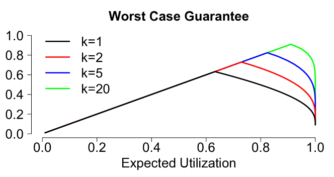
Figure 3: For any level of expected utilization achieved by a static threshold policy, our results imply a tight lower bound on the fraction of the prophet’s value obtained, shown above. For each $k$, this lower bound ($y$-axis) is maximized and equals $\gamma_{k}$ when the expected utilization ($x$-axis) equals $\gamma_{k}$.

For example, our results immediately imply that for $k>4$, any threshold in between the thresholds that we study also guarantees $\gamma_{k}$ times the prophet’s value. In addition, Lemma 3.2 can be used to provide guarantees for thresholds outside of this range. For example, if a particular threshold has been used repeatedly, then expected utilization at that threshold is easy to estimate from past data. Based on this expected utilization (and no other information about the value distributions $F_{i}$) we can use Lemmas 3.2 and 3.3 to obtain the performance bounds in Figure 3.

Perhaps even more interestingly, our approach could be used to analyze a general class of demand statistic policies. These policies are specified by a non-decreasing function $g:\mathbb{N}\to\mathbb{R}$ and a constant $\phi$, and choose the threshold $t$ so that $\operatorname*{\mathbb{E}}[g(D^{t})]=\phi$. In this paper, we focused on two such policies: one based on expected utilization with $g(d)=\min\{d/k,1\}$ and $\phi=\gamma_{k}$, and another based on expected demand with $g(d)=d$ and $\phi=k$.

All demand statistic policies inherit the advantage discussed in Section 5.1: they are robust to monotone transformations of values, and can be used when only proxies for value are available. Additionally, many organizations are already used to tracking statistics such as demand, utilization, and stockout frequency, and using these statistics to adjust their policies.

For these reasons, developing performance guarantees based on other demand statistics is a worthwhile direction for future work. Our Theorem 1.7 for Bernoulli optimization provides a useful starting point, since it simplifies the search for a worst-case demand distribution. One natural question is, which demand statistics $g$ are sufficient to deliver optimal guarantees, when paired with an appropriate choice of $\phi$? Earlier we showed that expected utilization is sufficient, and expected demand is sufficient when $k>4$. We now show that expected demand is insufficient as a demand statistic when $k\leq 4$, for any choice of $\phi$.

Proposition 5.1

For $k<5$ and any value of $\phi$, there exists an instance $(k,{\bf F})$ such that the performance of any $t$ such that $\operatorname*{\mathbb{E}}_{{\bf V}\sim{\bf F}}[D^{t}({\bf V})]=\phi$ is strictly less than $\gamma_{k}$ times the prophet’s value.

Proposition 5.1 is established in two cases. If $d<k$, then the policy fails on an instance where all valuations are deterministically equal to 1, in which case it accepts too few applicants. On the other hand, if $d>k$, then the adversary can create an instance where all values are zero, except for a single applicant who has an infinitesimal probability of having a non-zero value. In this case, the algorithm with target demand of $d$ accepts too many zero applicants, and risks being unable to accept the positive value when it occurs.

Despite this negative result, we note that setting expected demand equal to $k$ does provide an optimal guarantee if values are identically distributed (even for $k\leq 4$).

Proposition 5.2

If values are IID, then for any $k\geq 1$, the performance of any threshold such that expected demand is equal to $k$ is at least $\gamma_{k}$ times the prophet’s value.

Open question about another demand statistic. Another natural choice of demand statistic is $g(d)=\mathbbm{1}(d\geq k)$, in which case $\operatorname*{\mathbb{E}}[g(D^{t})]$ gives the “stockout probability” (probability of running out of items). When $k=1$, Ehsani et al. (2018) show that setting the stockout probability to $1-1/e$ provides an optimal guarantee of $\gamma_{1}=1-1/e$. In fact, when $k=1$, stockout probability is equivalent to expected utilization, so their algorithm coincides with our own. We propose the following generalization of their algorithm for $k>1$: set the threshold such that the stockout probability is equal to $\mathbb{P}(\mathrm{Pois}(k)\geq k)$. For large $k$, this means that the stockout probability is just slightly above $1/2$. This is a simple policy to explain and implement, and we conjecture that it also guarantees a $\gamma_{k}$ fraction of the prophet’s value.

6 Proof of Theorem 1.1

We begin with a preliminary result about Poisson random variables.

Lemma 6.1

For any $k\in\mathbb{N}$ and $\lambda\geq 0$, we have

$$k\operatorname*{\mathbb{E}}[\mathsf{UT}_{k}(\mathrm{Pois}(\lambda))]=\lambda\mathbb{P}(\mathrm{Pois}(\lambda)<k)+k\mathbb{P}(\mathrm{Pois}(\lambda)>k)=\lambda\operatorname*{\mathbb{E}}[\mathsf{AR}_{k}(\mathrm{Pois}(\lambda))].$$ (17)

Therefore,

$$\operatorname*{\mathbb{E}}[\mathsf{UT}_{k}(\mathrm{Pois}(k))]=\operatorname*{\mathbb{E}}[\mathsf{AR}_{k}(\mathrm{Pois}(k))]=\gamma_{k}.$$ (18)

Proof of Lemma 6.1.

For any random variable $D$, we have

$$k\operatorname*{\mathbb{E}}[\mathsf{UT}_{k}(D)]=\operatorname*{\mathbb{E}}[\min(D,k)]=k\mathbb{P}(D>k)+\operatorname*{\mathbb{E}}[D\mathbbm{1}(D\leq k)].$$ (19)

When $D$ is Poisson with mean $\lambda$,

$$\operatorname*{\mathbb{E}}[D\mathbbm{1}(D\leq k)]=\sum_{j=0}^{k}j\frac{e^{-\lambda}\lambda^{j}}{j!}=\lambda\mathbb{P}(\mathrm{Pois}(\lambda)<k).$$ (20)

Combining (19) and (20) yields the first equality in (17). Meanwhile, for any $\lambda\geq 0$,

$$\operatorname*{\mathbb{E}}[\mathsf{AR}_{k}(\mathrm{Pois}(\lambda))] =\operatorname*{\mathbb{E}}\left[\min\left(\frac{k}{\mathrm{Pois}(\lambda)+1},1\right)\right]$$

$$=\mathbb{P}(\mathrm{Pois}(\lambda)<k)+\sum_{j=k}^{\infty}\frac{k}{1+j}e^{-\lambda}\frac{\lambda^{j}}{j!}$$

$$=\mathbb{P}(\mathrm{Pois}(\lambda)<k)+\frac{k}{\lambda}\sum_{j=k}^{\infty}e^{-\lambda}\frac{\lambda^{j+1}}{(1+j)!}$$

$$=\mathbb{P}(\mathrm{Pois}(\lambda)<k)+\frac{k}{\lambda}\mathbb{P}(\mathrm{Pois}(\lambda)>k).$$

This establishes the second equality in (17). Substituting $\lambda=k$ into (17) immediately yields (18):

$$\operatorname*{\mathbb{E}}[\mathsf{UT}_{k}(\mathrm{Pois}(k))]=\operatorname*{\mathbb{E}}[\mathsf{AR}_{k}(\mathrm{Pois}(k))]=\mathbb{P}(\mathrm{Pois}(k)>k)+\mathbb{P}(\mathrm{Pois}(k)<k)=1-\mathbb{P}(\mathrm{Pois}(k)=k)=\gamma_{k}.$$

$\square$

We now prove Theorem 1.1, which follows immediately from Lemmas 6.2 and 6.3. For $k\in\mathbb{N}$ define

$$W_{k} =k\cdot\frac{\mathbb{P}(\mathrm{Pois}(k)<k)}{\mathbb{P}(\mathrm{Pois}(k)>k)}.$$ (21)

Lemma 6.2

On Example 1.2, the prophet’s value is at least $k+W_{k}-\frac{1+W_{k}}{n+1}$.

Proof of Lemma 6.2.

If there are no high-value applicants, the prophet earns a reward of $k$. If there is at least one high-value applicant, then the prophet earns a reward that is at least $k+nW_{k}-1$. This implies that the prophet’s expected reward is at least

$$k+(nW_{k}-1)\left(1-\left(1-\frac{1}{n^{2}}\right)^{n}\right) \geq k+(nW_{k}-1)\left(1-\frac{1}{1+1/n}\right)$$

$$=k+W_{k}-\frac{1+W_{k}}{n+1}.$$

The inequality uses the fact that for $p\in[0,1]$ and $n\in\mathbb{N}$, $(1+pn)(1-p)^{n}\leq 1$. $\square$

Lemma 6.3

On Example 1.2, the value of any static threshold algorithm is at most

$$\gamma_{k}(k+W_{k})+2kW_{k}(n^{-2/3}+n^{-1/3}).$$

Our proof uses the fact that if $N$ is a non-negative integer-valued random variable, then

$$\operatorname*{\mathbb{E}}[N]=\sum_{j=0}^{\infty}\mathbb{P}(N>j).$$ (22)

Proof of Lemma 6.3.

Clearly any algorithm should accept the high value of $nW_{k}$, so we can restrict our search to fixed-threshold algorithms parameterized by a probability $p\in[0,1]$ of accepting the lower value of 1. Then each of the $n$ agents is accepted by the threshold independently with probability $q=1/n^{2}+(1-1/n)^{2}p$, and the expected number of accepted agents is $\operatorname*{\mathbb{E}}[\min\{\mathrm{Bin}(n,q),k\}]$.

Conditional on an agent being accepted, the expectation of his or her value is

$$\frac{(1-1/n^{2})p}{1/n^{2}+(1-1/n^{2})p}\cdot 1+\frac{1/n^{2}}{1/n^{2}+(1-1/n^{2})p}\cdot nW_{k}\leq 1+\frac{W_{k}}{nq}.$$

Therefore, the expected value collected by any fixed-threshold algorithm is at most

$$\max_{q\in[1/n^{2},1]}\operatorname*{\mathbb{E}}[\min\{\mathrm{Bin}(n,q),k\}]\left(1+\frac{W_{k}}{nq}\right).$$ (23)

We now consider two cases: either $q>n^{-2/3}$ or $q\leq n^{-2/3}$. If $q>n^{-2/3}$, then $nq>n^{1/3}$ and hence the value of (23) is less than $k(W_{k}n^{-1/3}+1)=k+kW_{k}n^{-1/3}$. Furthermore, $\gamma_{k}>1/2$ and $W_{k}\geq k$ implies that $\gamma_{k}(k+W_{k})>k$. New AMaybe show $W_{k}>k$?

In the other case where $q\leq n^{-2/3}$, we note that

$$\operatorname*{\mathbb{E}}[\min\{\mathrm{Bin}(n,q),k\}] =\sum_{j=0}^{\infty}\mathbb{P}[\mathrm{Bin}(n,q)=j]\min\{j,k\}$$

$$\leq\sum_{j=0}^{\infty}\left(\mathbb{P}[\mathrm{Pois}(nq)=j]+\left|\mathbb{P}[\mathrm{Bin}(n,q)=j]-\mathbb{P}[\mathrm{Pois}(nq)=j]\right|\right)\min\{j,k\}$$

$$\leq\operatorname*{\mathbb{E}}[\min(\mathrm{Pois}(nq),k)]+2knq^{2},$$

where we have used Le Cam’s theorem to bound the total variation distance between a $\mathrm{Bin}(n,q)$ random variable and a $\mathrm{Pois}(nq)$ random variable. We conclude that the value of (23) is at most

$$\operatorname*{\mathbb{E}}[\min(\mathrm{Pois}(nq),k)]\left(1+\frac{W_{k}}{nq}\right)+2kW_{k}n^{-2/3}+2kn^{-1/3}.$$

We will show that the first term in this expression is maximized when $nq=k$. When $nq=k$, Lemma 6.1 implies that this term is equal to

$$\operatorname*{\mathbb{E}}[\mathsf{UT}_{k}(\mathrm{Pois}(k))]\left(k+W_{k}\right)=\gamma_{k}(k+W_{k}).$$

All that remains is to prove that the function $\operatorname*{\mathbb{E}}[\min(\mathrm{Pois}(\lambda),k)]\left(\frac{W_{k}}{\lambda}+1\right)$ is maximized at $\lambda=k$. We first note that

$$\frac{d}{d\lambda}\operatorname*{\mathbb{E}}[\min(\mathrm{Pois}(\lambda),k)] =\mathbb{P}(\mathrm{Pois}(\lambda)<k).$$ (24)

This follows from the following calculations (the first of which uses (22)):

$$\operatorname*{\mathbb{E}}[\min(\mathrm{Pois}(\lambda),k)] =\sum_{j=0}^{k-1}\mathbb{P}(\mathrm{Pois}(\lambda)>j)=k-\sum_{j=0}^{k-1}\mathbb{P}(\mathrm{Pois}(\lambda)\leq j).$$ (25)

$$\frac{d}{d\lambda}\mathbb{P}(\mathrm{Pois}(\lambda)\leq j) =\frac{d}{d\lambda}\sum_{i=0}^{j}\frac{e^{-\lambda}\lambda^{i}}{i!}=-\frac{e^{-\lambda}\lambda^{j}}{j!}=-\mathbb{P}(\mathrm{Pois}(\lambda)=j).$$ (26)

From (24), it follows that

$$\frac{d}{d\lambda}\operatorname*{\mathbb{E}}[\min(\mathrm{Pois}(\lambda) ,k)](1+W_{k}/\lambda)$$

$$=\mathbb{P}(\mathrm{Pois}(\lambda)<k)(1+W_{k}/\lambda)-\frac{W_{k}}{\lambda^{2}}\operatorname*{\mathbb{E}}[\min(\mathrm{Pois}(\lambda),k)]$$

$$=\mathbb{P}(\mathrm{Pois}(\lambda)<k)(1+W_{k}/\lambda)-\frac{W_{k}}{\lambda^{2}}\left(\lambda\mathbb{P}(\mathrm{Pois}(\lambda)<k)+k\mathbb{P}(\mathrm{Pois}(\lambda)>k)\right)$$

$$=\mathbb{P}(\mathrm{Pois}(\lambda)<k)-\frac{W_{k}}{\lambda^{2}}k\mathbb{P}(\mathrm{Pois}(\lambda)>k)$$

$$=\mathbb{P}(\mathrm{Pois}(\lambda)<k)\left(1-\frac{k^{2}}{\lambda^{2}}\frac{\mathbb{P}(\mathrm{Pois}(k)<k)}{\mathbb{P}(\mathrm{Pois}(k)>k)}\frac{\mathbb{P}(\mathrm{Pois}(\lambda)>k)}{\mathbb{P}(\mathrm{Pois}(\lambda)<k)}\right),$$ (27)

The first equality follows from (24), the second from Lemma 6.1, the third from canceling terms, and the fourth from the definition of $W_{k}$ in (21).

In (27), the derivative is clearly seen to be 0 when $\lambda=k$. Our goal is to show that the derivative is positive when $\lambda<k$, and negative when $\lambda>k$. First suppose that $\lambda<k$. Then

$$\frac{k^{2}}{\lambda^{2}}\frac{\mathbb{P}[\mathrm{Pois}(k)<k]}{\mathbb{P}[\mathrm{Pois}(k)>k]}\frac{\mathbb{P}[\mathrm{Pois}(\lambda)>k]}{\mathbb{P}[\mathrm{Pois}(\lambda)<k]} =\frac{\sum_{j>k}\lambda^{j-2}/j!}{\sum_{j>k}k^{j-2}/j!}\frac{\sum_{j<k}k^{j}/j!}{\sum_{j<k}\lambda^{j}/j!}$$

$$<(\frac{\lambda}{k})^{k-1}\frac{\sum_{j<k}k^{j}/j!}{\sum_{j<k}\lambda^{j}/j!}$$

$$=\frac{\sum_{j<k}\lambda^{j}(\frac{\lambda}{k})^{k-1-j}/j!}{\sum_{j<k}\lambda^{j}/j!}$$

which is at most 1 because each term $(\frac{\lambda}{k})^{k-1-j}$ in the numerator is at most 1, for $j=1,\ldots,k-1$. Substituting into (27), this shows that the derivative is positive when $\lambda<k$.

On the other hand, suppose that $\lambda>k$. Then we can similarly derive

$$\frac{k^{2}}{\lambda^{2}}\frac{\mathbb{P}[\mathrm{Pois}(k)<k]}{\mathbb{P}[\mathrm{Pois}(k)>k]}\frac{\mathbb{P}[\mathrm{Pois}(\lambda)>k]}{\mathbb{P}[\mathrm{Pois}(\lambda)<k]} >(\frac{\lambda}{k})^{k-1}\frac{\sum_{j<k}k^{j}/j!}{\sum_{j<k}\lambda^{j}/j!}$$

$$=\frac{\sum_{j<k}\lambda^{j}(\frac{\lambda}{k})^{k-1-j}/j!}{\sum_{j<k}\lambda^{j}/j!}$$

$$\geq 1.$$

Substituting into (27) shows that the derivative is negative when $\lambda>k$, completing the proof. $\square$

7 Proofs for Theorem 1.3

7.1 Proof of Lemma 3.2

We begin by defining

$$U(t,{\bf F})=\operatorname*{\mathbb{E}}\limits_{{\bf V}\sim{\bf F}}\left[\sum_{i=1}^{n}\max(V_{i}-t,0)\right]$$ (28)

Lemma 3.2 follows immediately from Lemmas 7.1 and 7.2.

Lemma 7.1

For all $k\in\mathbb{N}$, $t\in\mathbb{R}_{+}$ and all ${\bf F}$,

$$\mathcal{PHT}_{k}({\bf F})\leq\mathcal{LP}_{k}({\bf F})\leq t\cdot k+U(t,{\bf F}).$$

Proof of Lemma 7.1.

On any sample path, let $X_{i}\in\{0,1\}$ be the indicator for the prophet (who sees all value realizations up-front) accepting applicant $i$, for all $i$. Note that we always have $\sum_{i}X_{i}\leq k$. Therefore, defining $x_{i}:=\operatorname*{\mathbb{E}}[X_{i}]$ for all $i$ forms a feasible solution to the optimization problem defining $\mathcal{LP}_{k}({\bf F})$. Now, we have $\mathcal{PHT}_{k}({\bf F})=\operatorname*{\mathbb{E}}[\sum_{i}V_{i}X_{i}]=\sum_{i}x_{i}\operatorname*{\mathbb{E}}[V_{i}|X_{i}=1]$ by definition. However, $\operatorname*{\mathbb{E}}[V_{i}|X_{i}=1]$ can be no greater than the average value of $V_{i}$ over its top $x_{i}$’th quantile, which can be written as $\frac{1}{x_{i}}\int_{1-x_{i}}^{1}F^{-1}(z)dz$. Therefore,

$$\mathcal{PHT}_{k}({\bf F})\leq\sum_{i}x_{i}\frac{1}{x_{i}}\int_{1-x_{i}}^{1}F^{-1}(z)dz=\sum_{i}\int_{1-x_{i}}^{1}F^{-1}(z)dz$$

which is at most $\mathcal{LP}_{k}({\bf F})$ by the feasibility of $x_{1},\ldots,x_{n}$.

To show the second inequality, note that for any $t\in\mathbb{R}_{+}$, and any feasible solution $x_{1},\ldots,x_{n}$ to the optimization problem defining $\mathcal{LP}_{k}({\bf F})$ (i.e. satisfying $\sum_{i=1}^{n}x_{i}\leq k;\ x_{i}\geq 0\ \forall i$), its objective value satisfies

$$\sum_{i=1}^{n}\int_{1-x_{i}}^{1}F^{-1}(z)dz =\sum_{i=1}^{n}\int_{1-x_{i}}^{1}(F^{-1}(z)-t+t)dz$$ (29)

$$\leq\sum_{i=1}^{n}\int_{1-x_{i}}^{1}\max(F^{-1}(z)-t,0)dz+\sum_{i=1}^{n}\int_{1-x_{i}}^{1}t\cdot dz$$ (30)

$$\leq\sum_{i=1}^{n}\int_{0}^{1}\max(F^{-1}(z)-t,0)dz+t\sum_{i=1}^{n}x_{i}$$ (31)

$$\leq U(t,{\bf F})+tk.$$

where we have applied the definition of $U(t,{\bf F})$ and the final inequality uses the fact that $t\geq 0$ and $\sum_{i=1}^{n}x_{i}\leq k$. This completes the proof. $\square$

Lemma 7.2

For all $k\in\mathbb{N}$, $t\in\mathbb{R}_{+}$ and all ${\bf F}$,

$$\mathcal{ST}_{k}^{t}({\bf F})\geq t\cdot k\cdot\mathop{\operatorname*{\mathbb{E}}}_{{\bf V}\sim{\bf F}}\left[\mathsf{UT}_{k}(D^{t}({\bf V}))\right]+U(t,{\bf F})\mathop{\operatorname*{\mathbb{E}}}_{{\bf V}\sim{\bf F}}\left[\mathsf{AR}_{k}(D^{t}({\bf V}))\right].$$

In our proof, for fixed $t\in\mathbb{R}_{+}$ and $V\in\mathbb{R}_{+}^{n}$ we define

$$D_{i}^{t}(V) =\mathbbm{1}(V_{i}>t),$$ (32)

$$D^{t}({\bf V}) =\sum_{i=1}^{n}D_{i}(V),$$ (33)

$$D_{-i}^{t}(V) =D^{t}({\bf V})-D_{i}^{t}(V).$$ (34)

The following identity can be quickly verified by considering the cases $D^{t}({\bf V})<k$ and $D^{t}({\bf V})\geq k$:

$$\min(D^{t}({\bf V}),k)=\sum_{i}D_{i}^{t}(V)\mathsf{AR}_{k}(D_{-i}^{t}(V)).$$ (35)

This identity is also used in the proof of Lemma 4.1.

Proof of Lemma 7.2.

Throughout, we fix $t$ and $V$, and write $D,D_{i}$ and $D_{-i}$, leaving the dependence on $t$ and $V$ implicit.

Suppose that $D_{i}=1$. If competing demand $D_{-i}$ is less than $k$, then $i$ will certainly be accepted. Otherwise, $i$ is accepted with probability $k/(1+D_{-i})$. From this observation, we can lower bound the performance of any static threshold policy as follows.

$$\mathcal{ST}_{k}^{t}({\bf F}) =\mathbb{E}\left[\sum_{i=1}^{n}V_{i}D_{i}\mathsf{AR}_{k}(D_{-i})\right]$$

$$=\mathbb{E}\left[\sum_{i=1}^{n}\left(tD_{i}+\max(V_{i}-t,0)\right)\mathsf{AR}_{k}(D_{-i})\right]$$

$$=t\cdot\mathbb{E}\left[\sum_{i=1}^{n}D_{i}\mathsf{AR}_{k}(D_{-i})\right]+\mathbb{E}\left[\sum_{i=1}^{n}\max(V_{i}-t,0)\mathsf{AR}_{k}(D_{-i})\right]$$

$$=t\cdot\mathbb{E}\left[\min(D,k)\right]+\sum_{i=1}^{n}\mathbb{E}\left[\max(V_{i}-t,0)\right]\mathbb{E}\left[\mathsf{AR}_{k}(D_{-i})\right]$$

$$\geq t\cdot\mathbb{E}\left[\min(D,k)\right]+\sum_{i=1}^{n}\mathbb{E}\left[\max(V_{i}-t,0)\right]\operatorname*{\mathbb{E}}\left[\mathsf{AR}_{k}(D)\right]$$

$$=t\cdot k\cdot\operatorname*{\mathbb{E}}\left[\mathsf{UT}_{k}(D)\right]+U(t,{\bf F})\operatorname*{\mathbb{E}}\left[\mathsf{AR}_{k}(D)\right].$$

The fourth line uses (35), the fifth uses the fact that $D_{-i}$ and $V_{i}$ are independent, and the inequality uses the fact that $D\geq D_{-i}$ and $\mathsf{AR}_{k}$ is weakly decreasing. $\square$

7.2 Proof of Lemma 3.3

In this section we prove Lemma 3.3. Because the statement is trivially true if $n=1$, we assume $n\geq 2$ and consider the problem of re-optimizing the pair of probabilities $p_{1},p_{2}$ while holding all other probabilities fixed.

Let $D^{-}_{\textbf{p}}$ denote the sum of $n-2$ independent Bernoulli random variables with means $p_{3},\ldots,p_{n}$. We note that for any function $f:\mathbb{N}\rightarrow\mathbb{R}$,

$$\mathbb{E}[f(D_{\textbf{p}})] \!=\!(1\!-\!p_{1})(1\!-\!p_{2})\mathbb{E}[f(D_{\textbf{p}}^{-})]\!+\!(p_{1}(1\!-\!p_{2})\!+\!p_{2}(1\!-\!p_{1}))\mathbb{E}[f(1\!+\!D_{\textbf{p}}^{-})]\!+\!p_{1}p_{2}\mathbb{E}[f(2\!+\!D_{\textbf{p}}^{-})]$$

$$\!=\!\mathbb{E}[f(D_{\textbf{p}}^{-})]\!+\!(p_{1}\!+\!p_{2})\mathbb{E}[f(1\!+\!D_{\textbf{p}}^{-})\!-\!f(D_{\textbf{p}}^{-})]\!+\!p_{1}p_{2}\mathbb{E}[f(2\!+\!D_{\textbf{p}}^{-})\!+\!f(D_{\textbf{p}}^{-})\!-\!2f(1\!+\!D_{\textbf{p}}^{-})].$$ (36)

Note that the terms inside of the expectation operators do not depend on $p_{1}$ or $p_{2}$. This motivates the study of optimization problems of the following form.

$$\min \hskip 21.68121ptB_{0}+B_{1}(p_{1}+p_{2})+B_{2}p_{1}p_{2}$$ (37)

$$s.t. \hskip 21.68121ptA_{0}+A_{1}(p_{1}+p_{2})+A_{2}p_{1}p_{2}=\phi$$

$$\hskip 21.68121pt(p_{1},p_{2})\in[0,1]^{2}.$$

Lemma 7.3 gives structural results about the solution to this class of optimization problem.

Lemma 7.3

If the optimization problem (37) is feasible, then:

1. Any feasible solution in the interior $(0,1)^{2}$ with $p_{1}\neq p_{2}$ is suboptimal, unless all feasible solutions have the same objective value.

2. If $A_{2}=0,A_{1}\neq 0$, and $B_{2}<0$, then any solution with $p_{1}\neq p_{2}$ is suboptimal.

3. If $A_{2}\neq 0,A_{1}/A_{2}\leq-1$, and $B_{1}-B_{2}A_{1}/A_{2}<0$, then any solution with $p_{1}\neq p_{2}$ is suboptimal.

Proof of Lemma 7.3.

We prove the statements in Lemma 7.3 by analyzing several cases, depending on the values of the coefficients $A_{i}$ and $B_{i}$.

Case 1 addresses cases where the constraint is not quadratic ($A_{2}=0$), and is relevant for the proof of Statements 1 and 2. We divide this into two subcases: in Case 1a, the constraint is vacuous ($A_{1}=0$), while in 1b, it is linear.

Case 2 addresses cases where the constraint is quadratic ($A_{2}\neq 0$) and is relevant for the proof of Statements 1 and 3. Case 2a corresponds to a case where at least one of two terms (after a variable transformation) is constrained to be 0. Case 2b can be considered the “general” case in which no critical expressions are equal to $0$.

Case 1a: $A_{2}=0,A_{1}=0$. In this case, Statements 2 and 3 do not apply, so we prove only Statement 1. If (37) is feasible, then its equality constraint is redundant. Note that the gradient of the objective function at a point $(p_{1},p_{2})$ is $(B_{1}+B_{2}p_{2},B_{1}+B_{2}p_{1})$. If $(p_{1},p_{2})$ is a local minimum, then this gradient must equal $(0,0)$. This can only occur if $p_{1}=p_{2}$ or $B_{2}=B_{1}=0$ (in which case all feasible points are optimal). This establishes Statement 1 in case 1a.

Case 1b: $A_{2}=0,A_{1}\neq 0$. In this case, Statement 3 does not apply, so we prove only Statements 1 and 2. In this case, we have $p_{1}+p_{2}=(\phi-A_{0})/A_{1}$, which makes $B_{2}p_{1}p_{2}$ the only variable term in the objective function to be minimized. If $B_{2}<0$, then the objective value is strictly reduced by setting $p_{1}$ and $p_{2}$ to be equal. This proves Statement 2 in case 1b. If $B_{2}>0$, then the objective value is strictly reduced by setting at least one of $p_{1}$ or $p_{2}$ to be an extreme point in $\{0,1\}$. If $B_{2}=0$, then all feasible solutions have the same objective value. Combined, these arguments also establish Statement 1 in case 1b.

Case 2: $A_{2}\neq 0$. In this case, Statement 2 does not apply, so we prove only Statements 1 and 3. Define

$$q_{i} =p_{i}+A_{1}/A_{2}\text{ for }i\in\{1,2\};$$

$$\gamma =\frac{\phi-A_{0}}{A_{2}}+\frac{A_{1}^{2}}{A_{2}^{2}};$$

$$C_{0} =B_{0}-2B_{1}A_{1}/A_{2}+B_{2}(A_{1}/A_{2})^{2}+\gamma B_{2};$$

$$C_{1} =B_{1}-B_{2}A_{1}/A_{2}.$$

Then (37) can be reformulated as

$$\min \hskip 21.68121ptC_{0}+C_{1}(q_{1}+q_{2})$$

$$s.t. \hskip 21.68121ptq_{1}q_{2}=\gamma$$

$$\hskip 21.68121ptq_{1},q_{2}\in[A_{1}/A_{2},A_{1}/A_{2}+1].$$

Case 2a. $A_{2}\neq 0,\gamma=0$. At least one of $q_{1},q_{2}$ must be 0. WLOG assume $q_{1}=0$ and consider the optimization problem over $q_{2}\in[A_{1}/A_{2},A_{1}/A_{2}+1]$. If $C_{1}<0$, then the unique optimal solution is $q_{2}=A_{1}/A_{2}+1$ (i.e. $p_{2}=1$); if $C_{1}>0$, then the unique optimal solution is $q_{2}=A_{1}/A_{2}$ (i.e. $p_{2}=0$); if $C_{1}=0$, then all feasible solutions are optimal. Moreover, if $C_{1}<0$ and $A_{1}/A_{2}\leq-1$, then $\gamma=0$ is only feasible if $A_{1}/A_{2}=-1$, in which case the unique optimal solution is $q_{1}=q_{2}=0$ (corresponding to $p_{1}=p_{2}=1$). This establishes both Statements 1 and 3 in case 2a.

Case 2b. $A_{2}\neq 0,\gamma\neq 0$. In this case we cannot have $q_{1}=0$, so substitute $q_{2}=\gamma/q_{1}$, making the objective function $C_{0}+C_{1}(q_{1}+\gamma/q_{1})$. If $C_{1}=0$, then all feasible solutions are optimal. If $C_{1}\neq 0$, then the derivative of the objective can equal zero only if $1-\gamma/q_{1}^{2}=0$, in which case $q_{1}=q_{2}$ (and thus $p_{1}=p_{2}$). Therefore, there is no local minimum with $(p_{1},p_{2})\in(0,1)^{2}$ and $p_{1}\neq p_{2}$. It follows that when $C_{1}\neq 0$, any global minimum either has $p_{1}=p_{2}$ or lies on the boundary. This establishes Statement 1 in case 2b.

Turning to Statement 3, note that if $A_{1}/A_{2}\leq-1$, then $q_{1},q_{2}\leq 0$, so the problem is infeasible for $\gamma<0$. Thus, assume $\gamma>0$ and $q_{1},q_{2}<0$. The second derivative of the objective equals $2C_{1}\gamma/q_{1}^{3}$ which is strictly positive. By strict convexity, the unique global minimizer must arise at the local minimum where $q_{1}=-\sqrt{\gamma}$. Furthermore, if $q_{1}q_{2}=\gamma$ has a solution in $[A_{1}/A_{2},A_{1}/A_{2}+1]^{2}$, then it follows that $-\sqrt{\gamma}\in[A_{1}/A_{2},A_{1}/A_{2}+1]$, and therefore the global minimizer is feasible. This establishes Statement 3 in case 2b. $\square$

In what follows, we use several established facts about the sum of independent Bernoulli random variables, which we collect in the following lemma. New ACould state for $D_{\textbf{p}}$ or $D_{\textbf{p}}^{-}$. We use it for $D_{\textbf{p}}^{-}$, but it seems most elegant (but perhaps more confusing) to state using $D_{\textbf{p}}$.

Lemma 7.4

Fix $n\in\mathbb{N}$ and $\textbf{p}\in[0,1]^{n}$, and let $\lambda=\mathbb{E}[D_{\textbf{p}}]=\sum_{i=1}^{n}p_{i}$. For $j\in\mathbb{N}_{0}$, let $h_{j}=\mathbb{P}(D_{\textbf{p}}=j)$ and $H_{j}=\mathbb{P}(D_{\textbf{p}}\leq j)$. Then

1. The support $\{j:h_{j}>0\}$ is an interval.

2. The density $h$ is log-concave, meaning that for all $j\geq 1$,

   $$h_{j}^{2}\geq h_{j-1}h_{j+1}.$$

   Furthermore, this inequality is strict whenever $h_{j}>0$.

3. The density $h$ is unimodal, with mode $\in\{\lfloor\lambda\rfloor,\lceil\lambda\rceil\}$. That is,

   $$h_{0} \leq h_{1}\leq h_{2}\leq\cdots\leq h_{\lfloor\lambda\rfloor}$$

   $$h_{\lceil\lambda\rceil} \geq h_{\lceil\lambda\rceil+1}\geq h_{\lceil\lambda\rceil+2}\geq\cdots$$

4. For any $j\geq 2$,

   $$H_{j-2}h_{j-1}\leq H_{j-1}h_{j-2}.$$ (38)

Proof of Lemma 7.4.

The first fact is obvious. The second is shown by Samuels (1965), and the third is shown by several papers, including Darroch (1964), Samuels (1965), and Wang (1993). The final fact follows because if the distribution of $D_{\textbf{p}}$ is log-concave, then so is the distribution of $n-D_{\textbf{p}}$, and log-concave distributions have increasing hazard rates (see An (1995), Proposition 10).

New A Samuels (1965) explicitly notes log-concavity. Unimodality has been proven by Darroch (1964), Samuels (1965), Wang (1993).jogdeo-samuels_1968 shows that the median is either $\lfloor\lambda\rfloor$ or $\lceil\lambda\rceil$. Many general facts about the Poisson Binomial distribution (sum of independent Bernoullis) are summarized by boland_2007 and tang-tang_2019. baillon-cominetti-vaisman_2016 give a tight upper bound on its density function.

$\square$

Proof of Lemma 3.3.

If $\phi>1$, then the optimization problem is infeasible. If $\phi=1$, then the unique optimal solution is $p_{i}=1$ for all $i$. Therefore, we assume that $\phi<1$. It follows from the definition of $\mathsf{UT}$ in (4) that for any feasible solution,

$$\mathbb{P}(D_{\textbf{p}}\leq k-1)>0.$$ (39)

Furthermore, we claim that for any optimal solution, we must have

$$\mathbb{E}[\mathsf{AR}_{k}(D_{\textbf{p}})]<1.$$ (40)

This follows because $p_{i}=\phi/k$ for $i\in\{1,\ldots k\}$ and $p_{i}=0$ for $i>k$ is a feasible solution (that is, $\mathbb{E}[\mathsf{UT}_{k}(D_{\textbf{p}})]=\phi$) and satisfies (40).

Take a feasible solution ${\bf p}$ in which $p_{i}\neq p_{j}$. We will show that this solution is not optimal. Without loss of generality, relabel so that $i=1,j=2$, and consider optimizing $p_{1}$ and $p_{2}$ with all other probabilities fixed. Let $h$ and $H$ denote the density and CDF of the sum of variables $\{3,4,\ldots n\}$. We face an optimization problem in the form (37), with

$$A_{1} =\mathbb{E}[\mathsf{UT}_{k}(1+D^{-})-\mathsf{UT}_{k}(D^{-})] =H_{k-1}/k\,\,\,$$ (41)

$$A_{2} =\mathbb{E}[\mathsf{UT}_{k}(2+D^{-})+\mathsf{UT}_{k}(D^{-})-2\mathsf{UT}_{k}(1+D^{-})] =-h_{k-1}/k$$ (42)

$$B_{1} =\mathbb{E}[\mathsf{AR}_{k}(1+D^{-})-\mathsf{AR}_{k}(D^{-})]$$ (43)

$$B_{2} =\mathbb{E}[\mathsf{AR}_{k}(2+D^{-})+\mathsf{AR}_{k}(D^{-})-2\mathsf{AR}_{k}(1+D^{-})]$$ (44)

Note that the second equalities for $A_{1}$ and $A_{2}$ above follow from the observations

$$\mathsf{UT}_{k}(1+j)-\mathsf{UT}_{k}(j) =\frac{1}{k}\mathbbm{1}(j\leq k-1),$$

$$\mathsf{UT}_{k}(2+j)+\mathsf{UT}_{k}(j)-2\mathsf{UT}_{k}(1+j) =-\frac{1}{k}\mathbbm{1}(j=k-1).$$

Meanwhile, we have

$$\mathsf{AR}_{k}(1+j)-\mathsf{AR}_{k}(j) =\left\{\begin{array}[]{c l}0&j\leq k-2\\ \frac{-k}{(j+1)(j+2)}&j\geq k-1\end{array}\right.$$ (47)

$$\mathsf{AR}_{k}(2+j)+\mathsf{AR}_{k}(j)-2\mathsf{AR}_{k}(1+j) =\left\{\begin{array}[]{c l}0&j\leq k-3\\ \frac{-1}{k+1}&j=k-2\\ \frac{2k}{(j+1)(j+2)(j+3)}&j\geq k-1\end{array}\right.$$ (51)

We first consider the case where $A_{2}=0$, and then the case where $A_{2}\neq 0$.

Case 1. $A_{2}=0$. It follows from Lemma 7.4 part 1 that either

$$h_{j}=0\text{ for all }j\geq k-1,$$ (52)

or $h_{j}=0$ for all $j\leq k-1$. The latter case contradicts the feasibility constraint (39), so (52) must hold. It follows from (52) and (41) that $A_{1}=1/k$. Furthermore, (44) and (51) imply $B_{2}=-h_{k-2}/(k+1)\leq 0$. If $B_{2}=0$, then $h_{k-2}=0$, which further implies that $D_{\textbf{p}}$ is at most $k-1$ and that $\mathbb{E}[\mathsf{AR}_{k}(D_{\textbf{p}})]=1$. This contradicts the optimality condition (40). If $B_{2}<0$, then the second statement of Lemma 7.3 implies that p cannot be optimal.

Case 2. $A_{2}\neq 0$. By statement 3 of Lemma 7.3, p is sub-optimal if the following conditions hold:

$$A_{1}/A_{2}\leq-1$$ (53)

$$B_{1}-B_{2}A_{1}/A_{2}<0.$$ (54)

By (41) and (42), $A_{1}/A_{2}=-H_{k-1}/h_{k-1}\leq-1$, so (53) holds. All that remains is to show (54). For $j\in\mathbb{N}$, define

$$C_{j}=\frac{k(k+1)}{(j+1)(j+2)},$$

and note that

$$\frac{2k(k+1)}{(j+1)(j+2)(j+3)}=C_{j}-C_{j+1}.$$

By (41) and (42), $A_{2}\neq 0$ implies $H_{k-1}\geq h_{k-1}>0$. By (41), (42), (47) and (51), we have

$$(k+1)(B_{1}-B_{2}A_{1}/A_{2}) =-\sum_{j=k-1}^{\infty}C_{j}h_{j}+\frac{H_{k-1}}{h_{k-1}}\left(-h_{k-2}+\sum_{j=k-1}^{\infty}(C_{j}-C_{j+1})h_{j}\right)$$

$$=\frac{H_{k-2}}{h_{k-1}}\sum_{j=k-1}^{\infty}C_{j}h_{j}-\frac{H_{k-1}}{h_{k-1}}\left(h_{k-2}+\sum_{j=k-1}^{\infty}C_{j+1}h_{j}\right)$$

$$=\frac{H_{k-1}}{h_{k-1}}\left(\frac{H_{k-2}}{H_{k-1}}\sum_{j=k-1}^{\infty}C_{j}h_{j}-\sum_{j=k-2}^{\infty}C_{j+1}h_{j}\right)$$

$$=\frac{H_{k-1}}{h_{k-1}}\sum_{j=k-1}^{\infty}\left(\frac{H_{k-2}}{H_{k-1}}h_{j}-h_{j-1}\right)C_{j}$$ (55)

Part 4 of Lemma 7.4 implies that

$$\frac{H_{k-2}}{H_{k-1}}\leq\frac{h_{k-2}}{h_{k-1}},$$

and therefore each term in (55) is non-positive, with some term strictly negative. This implies that (54) holds, and therefore by Statement 3 in Lemma 7.3, that ${\bf p}$ cannot be optimal. New ARevisit this to explain why some term in (55) is strictly negative. $\square$

7.3 Proof of Lemma 3.4

Proof of Lemma 3.4.

Applying (22), we see that for any demand distribution $D$,

$$\operatorname*{\mathbb{E}}[\mathsf{UT}_{k}(D)]=\frac{1}{k}\operatorname*{\mathbb{E}}[\min(D,k)]=\frac{1}{k}\sum_{j=0}^{k-1}\mathbb{P}(D>j)=1-\frac{1}{k}\sum_{j=0}^{k-1}\mathbb{P}(D\leq j).$$

Theorem 4 in Hoeffding (1956) implies that for $j<k$, $\mathbb{P}(\mathrm{Bin}(n,k/n)\leq j)$ is decreasing in $n$, so

$$\operatorname*{\mathbb{E}}[\mathsf{UT}_{k}(\mathrm{Bin}(n,k/n)] \geq\lim_{n\rightarrow\infty}\operatorname*{\mathbb{E}}[\mathsf{UT}_{k}(\mathrm{Bin}(n,k/n)]$$

$$=\operatorname*{\mathbb{E}}[\mathsf{UT}_{k}(\mathrm{Pois}(k))]$$

$$=\gamma_{k}$$

$$=\operatorname*{\mathbb{E}}[\mathsf{UT}_{k}(\mathrm{Bin}(n,p_{n})],$$ (56)

where the first equality follows from Le Cam’s theorem, the second from Lemma 6.1, and third from the definition of $p_{n,k}$ in (9). Since $\mathsf{UT}_{k}$ is an increasing function, $\operatorname*{\mathbb{E}}[\mathsf{UT}_{k}(\mathrm{Bin}(n,p)]$ is increasing in $p$, so (56) implies that $p_{n,k}\leq k$, completing the proof. $\square$

8 Proofs for Theorems 1.6 and 1.7

8.1 Proof of Lemma 4.1

Proof of Lemma 4.1.

We fix a threshold $t\in\mathbb{R}_{+}$ and values $V\in\mathbb{R}_{+}^{n}$, and use $D$, $D_{i}$ and $D_{-i}$ as shorthand for $D^{t}({\bf V})$, $D_{i}^{t}(V)$ and $D_{-i}^{t}(V)$ as defined in (32), (33) and (34). We claim that

$$k\cdot\operatorname*{\mathbb{E}}\left[\mathsf{UT}_{k}(D)\right] =\operatorname*{\mathbb{E}}\left[\min(D,k)\right]$$

$$=\mathbb{E}\left[\sum_{i}D_{i}\mathsf{AR}_{k}(D_{-i})\right]$$

$$=\sum_{i}\mathbb{E}[D_{i}]\mathbb{E}\left[\mathsf{AR}_{k}(D_{-i})\right]$$

$$\geq\sum_{i}\mathbb{E}[D_{i}]\mathbb{E}\left[\mathsf{AR}_{k}(D)\right]$$

$$=\operatorname*{\mathbb{E}}[D]\operatorname*{\mathbb{E}}\left[\mathsf{AR}_{k}(D)\right].$$

The second line uses (35), the third uses independence of $D_{i}$ and $D_{-i}$, the inequality uses that $D\geq D_{-i}$ and $\mathsf{AR}_{k}$ is decreasing, and the final line follows from (33), which states that $D=\sum_{i}D_{i}$. Therefore, if $t$ is chosen so that $\operatorname*{\mathbb{E}}[D]=k$, it follows that $\operatorname*{\mathbb{E}}\left[\mathsf{UT}_{k}(D)\right]\geq\operatorname*{\mathbb{E}}\left[\mathsf{AR}_{k}(D)\right]$. $\square$

8.2 Proof of Theorem 1.7 and Lemma 4.2

Proof of Theorem 1.7.

Suppose for contradiction that all optimal solutions have at least two distinct non-{0,1} probabilities. Select an optimal solution p which maximizes the number of probabilities in {0,1}, which can be at most $n-2$ because there must exist indices $i,j$ for which $0<p_{i}<p_{j}<1$. Relabel these indices $i,j$ to be $1,2$, and consider the problem of optimizing $p_{1}$ and $p_{2}$, holding all others fixed. By (36), this is a version of the optimization problem (37). Because we have an interior optimal solution where the two probabilities are unequal, statement 1 of Lemma 7.3 implies that all feasible solutions must have the same objective value. Note that $p_{1}$ and $p_{2}$ can be modified to make one of them lie in $\{0,1\}$ while preserving feasibility. New AExplain preceding claim? This leads to an alternate optimal solution which has strictly more probabilities in {0,1}, causing a contradiction and completing the proof. $\square$

Proof of Lemma 4.2.

By Theorem 1.7, there exists an optimal solution in which each $p_{i}\in\{0,p,1\}$, for some $p\in(0,1)$. Thus, to prove Lemma 4.2, it suffices to show that any feasible solution which has this property and has $p_{i}=p,p_{j}=1$ for some $i,j$ is not optimal.

Without loss of generality, relabel so that $i=1$ and $j=2$. Consider the problem of optimizing over $p_{1}$ and $p_{2}$, holding the remaining probabilities fixed. This is a version of the optimization problem (37), in which $A_{1}=1,A_{2}=0$, and

$$B_{2}=\mathbb{E}[\mathsf{AR}_{k}(2+D^{-})+\mathsf{AR}_{k}(D^{-})-2\mathsf{AR}_{k}(1+D^{-})].$$

If $B_{2}<0$, then statement 2 in Lemma 7.3 implies that our solution is not optimal. Therefore, all that remains is to show that $B_{2}<0$. Note that

$$\mathsf{AR}_{k}(2+j)+\mathsf{AR}_{k}(j)-2\mathsf{AR}_{k}(1+j)=\left\{\begin{array}[]{c l}0&j\leq 3\\ \frac{-1}{k+1}&j=k-2\\ \frac{2k}{(j+1)(j+2)(j+3)}&j\geq k-1\end{array}\right.$$ (57)

For $j\geq k-1$ define

$$C_{j}=\frac{2k(k+1)}{(j+1)(j+2)(j+3)}=\frac{k(k+1)}{(j+1)(j+2)}-\frac{k(k+1)}{(j+2)(j+3)}.$$

Note that for $\ell\geq k-1$, we have

$$\sum_{j=\ell}^{\infty}C_{j}=\frac{k(k+1)}{(\ell+1)(\ell+2)}.$$ (58)

In particular, taking $\ell=k-1$ we see that the $C_{j}$ sum to one. By (57) we have

$$\mathbb{E}[\mathsf{AR}_{k}(2+D^{-})+\mathsf{AR}_{k}(D^{-})-2\mathsf{AR}_{k}(1+D^{-})]=\frac{1}{k+1}\left(-h_{k-2}+\sum_{j=k-1}^{\infty}C_{j}h_{j}\right).$$

Showing that this is negative is equivalent to showing that $h_{k-2}$ is larger than a $C_{j}$-weighted average of $h_{j}$ for $j\geq k-1$.

Because $p_{1}=p,p_{2}=1$, the constraint $\sum_{i=1}^{n}p_{i}=k$ implies that $\mathbb{E}[D^{-}]=k-1-p$. Therefore, Lemma 7.4 part 3 implies that

$$h_{j}\leq h_{k}\text{ for all }j\geq k.$$ (59)

From this and (58) we have

$$-h_{k-2}+\sum_{j=k-1}^{\infty}C_{j}h_{j} \leq-h_{k-2}+h_{k-1}C_{k-1}+h_{k}\sum_{j=k}^{\infty}C_{j}$$

$$=-h_{k-2}+\frac{2}{k+2}h_{k-1}+\frac{k}{k+2}h_{k}.$$ (60)

We wish to establish that this expression is negative. Because indexes with $p_{i}=0$ are irrelevant, we can assume without loss of generality that there are $n$ nonzero $p_{i}$. Let $d$ be the number of indices $i$ with $p_{i}=1$ in our initial solution, so $n-d$ is the number of indices with $p_{i}=p$. Because $n-d\geq 1$ by assumption and $\sum_{i}p_{i}=d+p(n-d)=k$, we must have

$$d \leq k-1,$$ (61)

$$p =\frac{k-d}{n-d}.$$ (62)

Because $D^{-}-(d-1)\sim Bin(n-d-1,p)$, for $j\in\{d-1,d-2,\ldots,n-2\}$ we have

$$h_{j}={n-d-1\choose j-d+1}p^{j-d+1}(1-p)^{n-j-2}$$ (63)

Noting that $d-1\leq k-2$ by (61), we can use (63) to rewrite the right side of (60) as

$${n-d-1\choose k-d}p^{k-d}(1-p)^{n-k-1}\left(-\frac{1-p}{p}\frac{k-d}{n-k}+\frac{2}{k+2}+\frac{k}{k+2}\frac{p}{1-p}\frac{n-k-1}{k-d+1}\right).$$

The sign of this expression is determined by the second term. Substituting (62) into this term, we see that it is equal to

$$-1+\frac{2}{k+2}+\frac{k}{k+2}\frac{n-k-1}{n-k}\frac{k-d}{k-d+1}.$$

This is clearly negative, as both fractions multiplying $\frac{k}{k+2}$ are strictly less than one. $\square$

8.3 Proof of Lemma 4.3 for $k>8$

We begin with two technical lemmas.

Lemma 8.1

For any $k,n\in\mathbb{N}$ with $k\leq n$, we have $\operatorname*{\mathbb{E}}[\mathsf{AR}_{k}(\mathrm{Bin}(n,\frac{k}{n}))]\geq 1-\varphi_{k}(n)$, where

$$\varphi_{k}(n)=\left(1-\frac{k}{n+1}\right)\mathbb{P}[\mathrm{Bin}(n,\frac{k}{n})=k]+\frac{1}{2(n+1)}.$$

Proof of Lemma 8.1.

We can derive that

$$\operatorname*{\mathbb{E}}[\mathsf{AR}_{k}(\mathrm{Bin}(n,k/n))] =\mathbb{P}[\mathrm{Bin}(n,k/n)<k]+\sum_{d=k}^{n}\frac{k}{d+1}\binom{n}{d}(k/n)^{d}(1-k/n)^{n-d}$$

$$=\mathbb{P}[\mathrm{Bin}(n,k/n)<k]+\frac{n}{n+1}\sum_{d=k}^{n}\frac{(n+1)!}{(d+1)!(n-d)!}(k/n)^{d+1}(1-k/n)^{n-d}$$

$$=\mathbb{P}[\mathrm{Bin}(n,k/n)<k]+\frac{n}{n+1}\mathbb{P}[\mathrm{Bin}(n+1,k/n)>k]$$ (64)

$$=\mathbb{P}[\mathrm{Bin}(n,k/n)<k]+\frac{n}{n+1}\left(\mathbb{P}[\mathrm{Bin}(n,k/n)>k]+\frac{k}{n}\mathbb{P}[\mathrm{Bin}(n,k/n)=k]\right)$$

$$=1-\frac{1}{n+1}\mathbb{P}[\mathrm{Bin}(n,k/n)>k]-\left(1-\frac{k}{n+1}\right)\mathbb{P}[\mathrm{Bin}(n,k/n)=k]$$

where the penultimate equality holds because by independence, $\mathrm{Bin}(n+1,k/n)>k$ if and only if either (i) there are at least $k$ successes in the first $n$ trials; or (ii) there are exactly $k$ successes in the first $n$ trials and the $n+1$’st trial is also successful. The proof is then completed by the fact that the median of a $\mathrm{Bin}(n,k/n)$ random variable is $k$, which implies that $\mathbb{P}[\mathrm{Bin}(n,k/n)>k]\leq 1/2$. $\square$

Lemma 8.2

For all integers $k\geq 1$, treating $\varphi_{k}(n)$ as a function over real numbers in $n\in[k,\infty)$, we have that for all $n\geq k+2$,

$$2(n+1)^{2}\varphi^{\prime}_{k}(n)\geq k\frac{e^{-k}k^{k}}{k!}(1-\frac{1}{n}-\frac{1}{n-k}-\frac{1}{n(n-k)})-1,$$ (65)

where the RHS of (65) in increasing in $n$.

Proof of Lemma 8.2.

Define $\psi_{k}(n)=(1-\frac{k}{n+1})\mathbb{P}[\mathrm{Bin}(n,\frac{k}{n})=k]$, which equals the first term in $\varphi_{k}(n)$. We can derive that

$$\psi_{k}(n) =\left(1-\frac{k}{n+1}\right)\frac{n(n-1)\cdots(n-k+1)}{k!}\frac{k^{k}}{n^{k}}\left(1-\frac{k}{n}\right)^{n-k}$$

$$=\frac{k^{k}}{k!}\left(1-\frac{k}{n+1}\right)\prod_{d=1}^{k-1}\left(1-\frac{d}{n}\right)\left(1-\frac{k}{n}\right)^{n-k}.$$

Therefore,

$$\ln\psi_{k}(n) =\ln\frac{k^{k}}{k!}+\ln(1-\frac{k}{n+1})+\sum_{d=1}^{k-1}\ln(1-\frac{d}{n})+(n-k)\ln(1-\frac{k}{n})$$

$$=\ln\frac{k^{k}}{k!}+\ln(n+1-k)-\ln(n+1)+\sum_{d=1}^{k-1}\ln(n-d)-(k-1)\ln n+(n-k)\ln(1-\frac{k}{n}).$$

Taking the $\ln$ of $\psi_{k}$ helps us evaluate its derivative:

$$\frac{1}{\psi_{k}(n)}\psi^{\prime}_{k}(n) =\frac{1}{n+1-k}-\frac{1}{n+1}+\sum_{d=1}^{k-1}\frac{1}{n-d}-\frac{k-1}{n}+\ln(1-\frac{k}{n})+(n-k)\frac{1}{1-k/n}\frac{k}{n^{2}}$$

$$=\frac{1}{n+1-k}-\frac{1}{n+1}+\sum_{d=1}^{k-1}\frac{1}{n-d}-\frac{k-1}{n}+\ln(1-\frac{k}{n})+\frac{k}{n}$$

$$=\frac{1}{n+1-k}-\frac{1}{n+1}+\sum_{d=1}^{k-1}\frac{1}{n-d}+\frac{1}{n}-\ln\frac{n}{n-k}$$

$$=\frac{k}{(n+1)(n-k+1)}-\left(\int_{n-k}^{n}\frac{1}{x}dx-\sum_{d^{\prime}=n-k+1}^{n}\frac{1}{d^{\prime}}\right).$$

Now, $\sum_{d^{\prime}=n-k+1}^{n}1/d^{\prime}$ represents a right Riemann sum for the integral $\int_{n-k}^{n}(1/x)dx$. Since $1/x$ is decreasing, the area under the curve $1/x$ from $x=d^{\prime}-1$ to $x=d^{\prime}$ is greater than $1/d^{\prime}$, for all $d^{\prime}=n-k+1,\ldots,n$. Moreover, since $1/x$ is convex, this difference is upper-bounded by the area of a triangle with base 1 and height $\frac{1}{d^{\prime}-1}-\frac{1}{d^{\prime}}$. Therefore,

$$\frac{1}{\psi_{k}(n)}\psi^{\prime}_{k}(n) \geq\frac{k}{(n+1)(n-k+1)}-\sum_{d^{\prime}=n-k+1}^{n}\frac{1}{2}(\frac{1}{d^{\prime}-1}-\frac{1}{d^{\prime}})$$

$$=\frac{k}{(n+1)(n-k+1)}-\left(\frac{1}{2(n-k)}-\frac{1}{2n}\right)$$

which implies that

$$\varphi^{\prime}_{k}(n) \geq\psi_{k}(n)\left(\frac{k}{(n+1)(n-k+1)}-\frac{k}{2n(n-k)}\right)-\frac{1}{2(n+1)^{2}}$$

$$=k\mathbb{P}[\mathrm{Bin}(n,k/n)=k]\left(1-\frac{k}{n+1}\right)\left(\frac{2n(n-k)-(n+1)((n-k)+1)}{2n(n-k)(n+1)(n-k+1)}\right)-\frac{1}{2(n+1)^{2}},$$

$$=k\mathbb{P}[\mathrm{Bin}(n,k/n)=k]\left(\frac{n+1-k}{n+1}\right)\left(\frac{n(n-k)-n-(n-k)-1}{2n(n-k)(n+1)(n-k+1)}\right)-\frac{1}{2(n+1)^{2}},$$

$$=\frac{1}{2(n+1)^{2}}\left(k\mathbb{P}[\mathrm{Bin}(n,k/n)=k]\frac{n(n-k)-n-(n-k)-1}{n(n-k)}-1\right).$$

We now use the fact that $\mathbb{P}[\mathrm{Bin}(n,k/n)=k]\geq e^{-k}k^{k}/k!$ to lower bound the expression in large parentheses by

$$k\frac{e^{-k}k^{k}}{k!}\left(1-\frac{1}{n}-\frac{1}{n-k}-\frac{1}{n(n-k)}\right)-1,$$

noting that $1-\frac{1}{n}-\frac{1}{n-k}-\frac{1}{n(n-k)}\geq 0$ when $n\geq k+2$. Therefore,

$$\varphi^{\prime}_{k}(n)\geq\frac{1}{2(n+1)^{2}}\left(k\frac{e^{-k}k^{k}}{k!}(1-\frac{1}{n}-\frac{1}{n-k}-\frac{1}{n(n-k)})-1\right),$$

where the expression is large parentheses is now clearly increasing in $n$. This completes the proof. $\square$

Lemma 8.3

Lemma 4.3 holds for $k\geq 31$.

Proof of Lemma 8.3.

Applying Lemma 8.2, since the RHS of (65) is increasing in $n$, we see that for all $n\geq k+2$, we have

$$2(n+1)^{2}\varphi^{\prime}_{k}(n)\geq k\frac{e^{-k}k^{k}}{k!}(1-\frac{1}{k+2}-\frac{1}{2}-\frac{1}{2(k+2)})-1,$$

whose RHS can be numerically verified to be positive for all $k\geq 31$. Therefore, $\varphi_{k}(n)$ is increasing over $n\geq k+2$ and we have that

$$\sup_{n\geq k+2}\varphi_{k}(n)=\lim_{n\to\infty}\varphi_{k}(n)=\frac{e^{-k}k^{k}}{k!}.$$ (66)

Meanwhile, by Lemma 8.1, we have that

$$\inf_{n\geq k}\operatorname*{\mathbb{E}}[\mathsf{AR}_{k}(\mathrm{Bin}(n,\frac{k}{n}))] \geq\min\{\operatorname*{\mathbb{E}}[\mathsf{AR}_{k}(\mathrm{Bin}(k,\frac{k}{k}))],1-\varphi_{k}(k+1),\inf_{n\geq k+2}(1-\varphi_{k}(n))\}$$

$$=\min\{\frac{k}{k+1},1-\frac{2}{k+2}\binom{k+1}{k}(\frac{k}{k+1})^{k}(\frac{1}{k+1})-\frac{1}{2(k+2)},1-\sup_{n\geq k+2}\varphi_{k}(n)\}$$

$$=\min\{1-\frac{1}{k+1},1-\frac{2}{k+2}(1-\frac{1}{k+1})^{k}-\frac{1}{2(k+2)},1-\frac{e^{-k}k^{k}}{k!}\}$$ (67)

where the final equality applies (66). From (67), the minimum can be numerically verified to equal the final argument for all $k\geq 31$, where we note that the first two arguments are $1-O(1/k)$ while the final argument is $1-O(1/\sqrt{k})$. $\square$

Lemma 8.4

Lemma 4.3 holds for $9\leq k\leq 30$.

Proof of Lemma 8.4.

Applying Lemma 8.2, since the RHS of (65) is increasing in $n$, we see that for all $n\geq k+11$, we have

$$2(n+1)^{2}\varphi^{\prime}_{k}(n)\geq k\frac{e^{-k}k^{k}}{k!}(1-\frac{1}{k+11}-\frac{1}{11}-\frac{1}{11(k+11)})-1,$$

whose RHS can be numerically verified to be positive for all $k\geq 9$. This demonstrates that $\varphi_{k}(n)$ is increasing over $n\geq k+11$. However in fact, $\varphi_{k}(n)$ is increasing over integers $n\geq k+1$, for all $9\leq k\leq 30$, as we numerically demonstrate in the table of values in Figure 4. Therefore, for all $9\leq k\leq 30$, we have

$$\sup_{n\geq k+1}\varphi_{k}(n)=\lim_{n\to\infty}\varphi_{k}(n)=\frac{e^{-k}k^{k}}{k!},$$

and applying Lemma 8.1, this implies that

$$\inf_{n\geq k}\operatorname*{\mathbb{E}}[\mathsf{AR}_{k}(\mathrm{Bin}(n,\frac{k}{n}))] \geq\min\{\operatorname*{\mathbb{E}}[\mathsf{AR}_{k}(\mathrm{Bin}(k,\frac{k}{k}))],\inf_{n\geq k+1}(1-\varphi_{k}(n))\}$$

$$=\min\{\frac{k}{k+1},1-\frac{e^{-k}k^{k}}{k!}\}.$$

The minimum can be numerically verified to equal the final argument for all $9\leq k\leq 30$.

Figure 4: Values of $\varphi_{k}(k+\ell)$, for all $9\leq k\leq 30$ and $1\leq\ell\leq 11$. Note that the values in every row, which correspond to a fixed $k$, are increasing.

$k$	$\ell=1$	$\ell=2$	$\ell=3$	$\ell=4$	$\ell=5$	$\ell=6$	$\ell=7$	$\ell=8$	$\ell=9$	$\ell=10$	$\ell=11$
9	0.1159	0.1164	0.1179	0.1193	0.1206	0.1216	0.1225	0.1233	0.1239	0.1245	0.1250
10	0.1059	0.1068	0.1086	0.1102	0.1116	0.1128	0.1138	0.1147	0.1154	0.1161	0.1167
11	0.0975	0.0987	0.1006	0.1024	0.1039	0.1052	0.1063	0.1073	0.1081	0.1088	0.1095
12	0.0904	0.0917	0.0938	0.0956	0.0973	0.0986	0.0998	0.1008	0.1017	0.1025	0.1032
13	0.0842	0.0857	0.0878	0.0897	0.0914	0.0928	0.0941	0.0951	0.0961	0.0969	0.0976
14	0.0788	0.0804	0.0826	0.0845	0.0862	0.0877	0.0890	0.0901	0.0910	0.0919	0.0927
15	0.0741	0.0758	0.0779	0.0799	0.0816	0.0831	0.0844	0.0855	0.0865	0.0874	0.0882
16	0.0699	0.0716	0.0738	0.0758	0.0775	0.0790	0.0803	0.0814	0.0825	0.0834	0.0842
17	0.0662	0.0679	0.0701	0.0720	0.0738	0.0753	0.0766	0.0777	0.0788	0.0797	0.0805
18	0.0628	0.0645	0.0667	0.0687	0.0704	0.0719	0.0732	0.0744	0.0754	0.0763	0.0772
19	0.0597	0.0615	0.0636	0.0656	0.0673	0.0688	0.0701	0.0713	0.0723	0.0733	0.0741
20	0.0570	0.0588	0.0609	0.0628	0.0645	0.0660	0.0673	0.0684	0.0695	0.0704	0.0713
21	0.0545	0.0562	0.0583	0.0602	0.0619	0.0633	0.0647	0.0658	0.0669	0.0678	0.0687
22	0.0522	0.0539	0.0560	0.0578	0.0595	0.0609	0.0622	0.0634	0.0644	0.0654	0.0662
23	0.0501	0.0518	0.0538	0.0556	0.0573	0.0587	0.0600	0.0612	0.0622	0.0631	0.0640
24	0.0481	0.0498	0.0518	0.0536	0.0552	0.0567	0.0579	0.0591	0.0601	0.0610	0.0619
25	0.0463	0.0480	0.0499	0.0517	0.0533	0.0547	0.0560	0.0571	0.0581	0.0591	0.0599
26	0.0446	0.0463	0.0482	0.0500	0.0515	0.0529	0.0542	0.0553	0.0563	0.0572	0.0581
27	0.0431	0.0447	0.0466	0.0483	0.0499	0.0512	0.0525	0.0536	0.0546	0.0555	0.0564
28	0.0416	0.0432	0.0451	0.0468	0.0483	0.0497	0.0509	0.0520	0.0530	0.0539	0.0547
29	0.0403	0.0419	0.0437	0.0453	0.0468	0.0482	0.0494	0.0505	0.0515	0.0524	0.0532
30	0.0390	0.0406	0.0423	0.0440	0.0455	0.0468	0.0480	0.0491	0.0500	0.0509	0.0517

$\square$

9 Proofs of Proposition 5.1 and Proposition 5.2

Proof of Proposition 5.1.

We prove this result in two cases. If $\phi<k$, then we can consider the degenerate case in which each variable is identically one. In this case, the static threshold policy accepts each item with probability $\phi/n$, and its expected value is the expected number of accepted items, which is $\operatorname*{\mathbb{E}}[\min(k,\mathrm{Bin}(n,\phi/n))]$. As $n$ grows, the fact that $\phi<k$ implies that this value converges to a constant strictly less than $k\cdot\gamma_{k}$. Meanwhile, the prophet’s value is equal to $k$.

If $\phi>k$, then we can consider the case in which $n-1$ values are identically zero, and the remaining value is $n$ with probability $1/n$, and zero otherwise. Then the prophet’s value is one. Meanwhile, when $n$ is large, the static threshold policy accepts each zero value item with probability approximately $\phi/n$, implying that demand is approximately Poisson distributed with mean $\phi$. It follows that when there is an item of value $n$, it is accepted with probability approximately $\operatorname*{\mathbb{E}}[\min(1,\frac{\phi}{1+\mathrm{Pois}(d)})]$, which is strictly less than $\gamma_{k}$ because $\phi>k\cdot\gamma_{k}$. $\square$

Proof of Proposition 5.2.

Throughout, let $F$ denote the distribution from which each $V_{i}$ is drawn, and let $t$ denote a threshold such that expected demand is equal to $k$. This algorithm keeps $\min(D^{t}({\bf V}),k)$ values, each with expected value $\mathbb{E}_{{\bf V}\sim F}[V|V>t]$. Meanwhile, by Lemma 7.1, $\mathcal{PHT}_{k}({\bf F})\leq tk+U(t,{\bf F})=k\cdot\mathbb{E}_{{\bf V}\sim F}[V|V>t]$. Combining these, we see that

$$\frac{\mathcal{TD}_{k}({\bf F})}{\mathcal{PHT}_{k}({\bf F})}\geq\frac{\mathbb{E}[\min(D_{t}(V),k)]\cdot\mathbb{E}_{{\bf V}\sim F}[V|V>t]}{k\cdot\mathbb{E}_{{\bf V}\sim F}[V|V>t]}=\frac{\mathbb{E}[\min(\mathrm{Bin}(n,k/n),k)]}{k},$$

where we have used the fact that $D^{t}({\bf V})\sim\mathrm{Bin}(n,k/n)$. By Le Cam’s theorem, as $n\rightarrow\infty$, $\mathrm{Bin}(n,k/n)\rightarrow\mathrm{Pois}(k)$, and the ratio above converges to $\operatorname*{\mathbb{E}}[\min(\mathrm{Pois}(k),k)]/k$, which equals $\gamma_{k}$ by Lemma 6.1. $\square$

References

- Agrawal et al. (2020) Agrawal S, Sethuraman J, Zhang X (2020) On optimal ordering in the optimal stopping problem. Proceedings of the 21st ACM Conference on Economics and Computation, 187–188.
- Alaei (2011) Alaei S (2011) Bayesian combinatorial auctions: Expanding single buyer mechanisms to many buyers. 2011 IEEE 52nd Annual Symposium on Foundations of Computer Science, 512–521 (IEEE Computer Society).
- Alaei (2014) Alaei S (2014) Bayesian combinatorial auctions: Expanding single buyer mechanisms to many buyers. SIAM Journal on Computing 43(2):930–972.
- Alaei et al. (2012) Alaei S, Taghi Hajiaghayi M, Liaghat V (2012) Online prophet-inequality matching with applications to ad allocation. ACM Conference on Economics and Computation (EC) .
- An (1995) An MY (1995) Log-concave probability distributions: Theory and statistical testing. Duke University Dept of Economics Working Paper (95-03).
- Arlotto and Gurvich (2019) Arlotto A, Gurvich I (2019) Uniformly bounded regret in the multisecretary problem. Stochastic Systems 9(3):231–260.
- Azar et al. (2014) Azar PD, Kleinberg R, Weinberg SM (2014) Prophet inequalities with limited information. Proceedings of the twenty-fifth annual ACM-SIAM symposium on Discrete algorithms, 1358–1377 (SIAM).
- Azar et al. (2018) Azar Y, Chiplunkar A, Kaplan H (2018) Prophet secretary: Surpassing the 1-1/e barrier. ACM Conference on Economics and Computation (EC) .
- Babaioff et al. (2007a) Babaioff M, Immorlica N, Kempe D, Kleinberg R (2007a) A knapsack secretary problem with applications. Approximation, randomization, and combinatorial optimization. Algorithms and techniques, 16–28 (Springer).
- Babaioff et al. (2007b) Babaioff M, Immorlica N, Kleinberg R (2007b) Matroids, secretary problems, and online mechanisms. Symposium on Discrete Algorithms (SODA’07), 434–443.
- Beyhaghi et al. (2021) Beyhaghi H, Golrezaei N, Leme RP, Pál M, Sivan B (2021) Improved revenue bounds for posted-price and second-price mechanisms. Operations Research 69(6):1805–1822.
- Bray (2019) Bray R (2019) Does the multisecretary problem always have bounded regret? Available at SSRN 3497056 .
- Cayley (1875) Cayley A (1875) Mathematical questions with their solutions. The Educational Times 23:18–19.
- Chawla et al. (2020) Chawla S, Devanur N, Lykouris T (2020) Static pricing for multi-unit prophet inequalities.
- Cominetti et al. (2010) Cominetti R, Correa JR, Rothvoß T, Martín JS (2010) Optimal selection of customers for a last-minute offer. Operations research 58(4-part-1):878–888.
- Correa et al. (2019a) Correa J, Dütting P, Fischer F, Schewior K (2019a) Prophet inequalities for iid random variables from an unknown distribution. Proceedings of the 2019 ACM Conference on Economics and Computation, 3–17.
- Correa et al. (2017) Correa J, Foncea P, Hoeksma R, Oosterwijk T, Vredeveld T (2017) Posted price mechanisms for a random stream of customers. ACM Conference on Economics and Computation (EC) .
- Correa et al. (2018) Correa J, Foncea P, Hoeksma R, Oosterwijk T, Vredeveld T (2018) Recent developments in prophet inequalities. ACM Sigecom Exchanges 17(1):61–70.
- Correa et al. (2019b) Correa J, Foncea P, Pizarro D, Verdugo V (2019b) From pricing to prophets, and back! Operations Research Letters 47(1):25–29.
- Correa et al. (2021) Correa J, Pizarro D, Verdugo V (2021) Optimal revenue guarantees for pricing in large markets. International Symposium on Algorithmic Game Theory, 221–235 (Springer).
- Correa et al. (2020) Correa J, Saona R, Ziliotto B (2020) Prophet secretary through blind strategies. Mathematical Programming .
- Darroch (1964) Darroch J (1964) On the distribution of the number of successes in independent trials. Annals of Mathematical Statistics 35:1317–1321.
- Dutting et al. (2020) Dutting P, Feldman M, Kesselheim T, Lucier B (2020) Prophet inequalities made easy: Stochastic optimization by pricing nonstochastic inputs. SIAM Journal on Computing 49(3):540–582.
- Dütting et al. (2016) Dütting P, Fischer F, Klimm M (2016) Revenue gaps for static and dynamic posted pricing of homogeneous goods. arXiv preprint arXiv:1607.07105 .
- Dynkin (1963) Dynkin EB (1963) The optimum choice of the instant for stopping a markov process. Soviet Mathematics 4:627–629.
- Ehsani et al. (2018) Ehsani S, Hajiaghayi M, Kesselheim T, Singla S (2018) Prophet secretary for combinatorial auctions and matroids. Proceedings of the twenty-ninth annual acm-siam symposium on discrete algorithms, 700–714 (SIAM).
- Esfandiari et al. (2017) Esfandiari H, Hajiaghayi M, Liaghat V, Monemizadeh M (2017) Prophet secretary. SIAM Journal on Discrete Mathematics 31(3):1685–1701.
- Ezra et al. (2020) Ezra T, Feldman M, Gravin N, Tang ZG (2020) Secretary matching with general arrivals. arXiv preprint arXiv:2011.01559 .
- Ezra et al. (2021) Ezra T, Feldman M, Gravin N, Tang ZG (2021) Prophet matching with general arrivals. Mathematics of Operations Research .
- Feldman et al. (2021) Feldman M, Svensson O, Zenklusen R (2021) Online contention resolution schemes with applications to bayesian selection problems. SIAM Journal on Computing 50(2):255–300.
- Ferguson (1989) Ferguson TS (1989) Who solved the secretary problem? Statistical science 4(3):282–289.
- Gallego et al. (2015) Gallego G, Li A, Truong VA, Wang X (2015) Online resource allocation with customer choice. arXiv preprint arXiv:1511.01837 .
- Ghosh and Kleinberg (2016) Ghosh A, Kleinberg R (2016) Optimal contest design for simple agents. ACM Transactions on Economics and Computation 4(4).
- Gilbert and Mosteller (1966) Gilbert JP, Mosteller F (1966) Recognizing the maximum of a sequence. Journal of the American Statistical Association 61(313):35–73.
- Hajiaghayi et al. (2007) Hajiaghayi MT, Kleinberg R, Sandholm T (2007) Automated online mechanism design and prophet inequalities. Proceedings of the 22nd National Conference on Artificial Intelligence (AAAI) 1:58–65.
- Hill (1983) Hill T (1983) Prophet inequalities and order selection in optimal stopping problems. Proceedings of the American Mathematical Society 88(1):131–137.
- Hill and Kertz (1982) Hill T, Kertz RP (1982) Comparisons of stop rule and supremum expectations of iid random variables. The Annals of Probability 10(2):336–345.
- Hill and Hordijk (1985) Hill TP, Hordijk A (1985) Selection of order of observation in optimal stopping problems. Journal of applied probability 22(1):177–184.
- Hill and Kertz (1992) Hill TP, Kertz RP (1992) A survey of prophet inequalities in optimal stopping theory. Contemp. Math 125:191–207.
- Hoeffding (1956) Hoeffding W (1956) On the distribution of the number of successes in independent trials. Annals of Mathematical Statistics 27:713–721.
- Jiang et al. (2022) Jiang J, Ma W, Zhang J (2022) Tight guarantees for multi-unit prophet inequalities and online stochastic knapsack. Proceedings of the 2022 Annual ACM-SIAM Symposium on Discrete Algorithms (SODA), 1221–1246 (SIAM).
- Kleinberg (2005) Kleinberg R (2005) A multiple-choice secretary algorithm with applications to online auctions. ACM Symposium on Discrete Algorithms (SODA) .
- Kleinberg and Weinberg (2012) Kleinberg R, Weinberg SM (2012) Matroid prophet inequalities. Proceedings of the forty-fourth annual ACM symposium on Theory of computing, 123–136.
- Krengel and Sucheston (1977) Krengel U, Sucheston L (1977) Semiamarts and finite values. Bulletin of the American Mathematical Society 83(4):745–747.
- Krengel and Sucheston (1978) Krengel U, Sucheston L (1978) On semiamarts, amarts, and processes with finite value. Probability on Banach spaces 4:197–266.
- Lee and Singla (2018) Lee E, Singla S (2018) Optimal online contention resolution schemes via ex-ante prophet inequalities. arXiv preprint arXiv:1806.09251 .
- Lieber (2021) Lieber R (2021) How to get the coronavirus vaccine in new york city. The New York Times March 22(https://www.nytimes.com/article/nyc-vaccine-shot.html).
- Lucier (2017) Lucier B (2017) An economic view of prophet inequalities. ACM SIGecom Exchanges 16(1):24–47.
- Rubinstein (2016) Rubinstein A (2016) Beyond matroids: Secretary problem and prophet inequality with general constraints. Proceedings of the forty-eighth annual ACM symposium on Theory of Computing, 324–332.
- Rubinstein et al. (2020) Rubinstein A, Wang JZ, Weinberg SM (2020) Optimal single-choice prophet inequalities from samples. 11th Innovations in Theoretical Computer Science Conference.
- Rubinstein (2021) Rubinstein D (2021) After unused vaccines are thrown in trash, cuomo loosens rules. The New York Times January 10(https://www.nytimes.com/2021/01/10/nyregion/new-york-vaccine-guidelines.html).
- Samuel-Cahn (1984) Samuel-Cahn E (1984) Comparison of threshold stop rules and maximum for independent nonnegative random variables. the Annals of Probability 1213–1216.
- Samuels (1965) Samuels S (1965) On the number of successes in independent trials. Annals of Mathematical Statistics 36:1272–1278.
- Wang (1993) Wang Y (1993) On the number of successes in independent trials. Statistica Sinica 3:295–312.
- Yan (2011) Yan Q (2011) Mechanism design via correlation gap. Proceedings of the twenty-second annual ACM-SIAM symposium on Discrete Algorithms, 710–719 (SIAM).