Convergence of position-dependent MALA with application to conditional simulation in GLMMs

Abstract

We establish conditions under which Metropolis-Hastings (MH) algorithms with a position-dependent proposal covariance matrix will or will not have the geometric rate of convergence. Some of the diffusions based MH algorithms like the Metropolis adjusted Langevin algorithm (MALA) and the pre-conditioned MALA (PCMALA) have a position-independent proposal variance. Whereas, for other modern variants of MALA like the manifold MALA (MMALA) that adapt to the geometry of the target distributions, the proposal covariance matrix changes in every iteration. Thus, we provide conditions for geometric ergodicity of different variations of the Langevin algorithms. These results have important practical implications as these provide crucial justification for the use of asymptotically valid Monte Carlo standard errors for Markov chain based estimates. The general conditions are verified in the context of conditional simulation from the two most popular generalized linear mixed models (GLMMs), namely the binomial GLMM with the logit link and the Poisson GLMM with the log link. Empirical comparison in the framework of some spatial GLMMs shows that the computationally less expensive PCMALA with an appropriately chosen pre-conditioning matrix may outperform the MMALA.

Key words: Drift conditions; Geometric ergodicity; Langevin diffusion; Markov chain; Metropolis-Hastings; Mixed models

1 Introduction

In physics, statistics, and several other disciplines one often deals with a complex probability density $f(x)$ on $\mathbb{R}^{d}$ that is available only up to a normalizing constant. Generally, the goal is to estimate ${\mathrm{E}}_{f}[g]:=\int_{\mathbb{R}^{d}}g(x)f(x)dx$ for some real valued function $g$. Markov chain Monte Carlo (MCMC) is the most popular method for sampling from such a $f$ and for providing a Monte Carlo estimate of $E_{f}[g]$ (Robert and Casella, 2004). In MCMC, a Markov chain $\{X_{n}\}$, which has $f$ as its stationary density, is run for a certain number of iterations, and ${\mathrm{E}}_{f}[g]$ is estimated by the sample average $\bar{g}_{n}:=\sum_{i=1}^{n}g(X_{i})/n$. Among the different MCMC algorithms, Metropolis-Hastings (MH) algorithms (Metropolis et al., 1953; Hastings, 1970) are predominant. In MH algorithms, given the current state $x$, a proposal $y$ is drawn from a density $q(x,y)$, which is then accepted with a certain probability. The accept-reject step guarantees reversibility of the Markov chain with respect to the target $f$, and, in turn, ensures stationarity. Besides, the acceptance probability generally does not involve the unknown normalizing constant in $f$, making the implementation of MH algorithms practically feasible.

A popular MH algorithm is the random walk Metropolis (RWM) where the proposal density is $N(x,hI_{d})$, the normal density centered at the current state $x$ and with the covariance matrix $hI_{d}$ for some $h>0$. A nice feature of the RWM is that the acceptance probability can be adjusted by choosing the step-size (proposal variance) $h$ accordingly. Indeed, lower step-size results in a higher acceptance probability but then the RWM chain takes longer to move around the space. Therefore, in higher dimensions, that is when $d$ is large, the Metropolis adjusted Langevin algorithm (MALA) (Rossky et al., 1978; Besag, 1994; Roberts and Tweedie, 1996a), which employs the gradient of log of the target distribution, is developed to achieve faster mixing. Since the mean of the proposal density $N(x+h\nabla\log f(x)/2,hI_{d})$ of the MALA is governed by the gradient information, it is likely to make moves in the directions in which $f$ is increasing. Thus, large proposals can be accepted with a higher probability, leading to high mixing of the Markov chain. On the other hand, the proposal density in the RWM does not make use of the structure of the target density. Superiority of the MALA over the RWM in terms of mixing time is demonstrated by Roberts and Rosenthal (1998) (see also Christensen et al., 2005; Dwivedi et al., 2019; Chen et al., 2020; Lee et al., 2020; Wu et al., 2021).

However, MALA may be inefficient when the coordinates of $x$ are highly correlated, and have largely differing marginal variances. In such situations, the step-size is compromised to accommodate the coordinates with the smallest variance. Such a situation arises when modeling spatially correlated data. Spatial models take the correlation of different locations into consideration, usually, the closer the two locations, the more similarity and the higher correlations they have. The pre-conditioned MALA (PCMALA) (Stramer and Roberts, 2007) is introduced to circumvent these issues by multiplying a covariance matrix to the gradient of log of the target density. The proposal density of the PCMALA is $N(x+hG\nabla\log f(x)/2,hG)$, while the selection of an appropriate covariance matrix requires further study. Without the Metropolis step, the MALA and the PCMALA degenerate to the unadjusted Langevin algorithm (ULA) (Parisi, 1981; Grenander and Miller, 1994; Roberts and Tweedie, 1996a) and the pre-conditioned ULA (PCULA), respectively, which although might converge to undesired distributions, require less computational time.

By taking into account the geometry of the target distribution in the selection of step-sizes, efficient versions of MALA can be formed that adapt to the characteristics of the target. Indeed, using ideas from both Riemannian and information geometry, Girolami and Calderhead (2011) propose a generalization of MALA, called the manifold MALA (MMALA). MMALA is constructed taking into account the natural geometry of the target density and considering a Langevin diffusion on a Riemann manifold. In the MMALA, the covariance matrix $G$, unlike the PCMALA, changes in every iteration. More recently, Xifara et al. (2014) propose the position-dependent MALA (PMALA). There are other works in the literature (see e.g Haario et al., 2001; Roberts and Rosenthal, 2009), which consider RWM algorithms where the Gaussian proposal distribution is centered at the current state and the covariance matrix depends on the current or a finite number of previous states.

A Harris ergodic Markov chain will converge to the target distribution, and ${\mathrm{E}}_{f}[g]$ can be consistently estimated by the sample mean $\bar{g}_{n}$ (Meyn and Tweedie, 1993). On the other hand, in practice, it is important to ascertain the errors associated with the estimate $\bar{g}_{n}$. Establishing geometric ergodicity of a Markov chain is the most standard method for guaranteeing a central limit theorem (CLT) for $\bar{g}_{n}$ and finding its standard errors. Thus, the geometric rate of convergence for Markov chains is highly desired. Furthermore, a non-geometrically ergodic chain may sample heavily from the tails instead of the center of the distribution, leading to instability of the Monte Carlo estimation (Roberts and Tweedie, 1996b). The main contribution of this article is that it establishes conditions under which geometric ergodicity will and will not hold for the position-dependent MALA. Indeed, we provide these results for MH algorithms where the normal proposal density has a general mean function $c(x)$ and a covariance matrix $G(x)$ depending on the current position $x$ of the Markov chain. As special cases, these results also hold for the MMALA, the PMALA, and the PCMALA. We also provide conditions guaranteeing geometric ergodicity of the PCULA. Our results will help practitioners implementing these MCMC algorithms to choose appropriate step-sizes ensuring the geometric convergence rates. Previously, Roberts and Tweedie (1996b) derive conditions under which the MALA and ULA chains are geometrically ergodic (GE). However, in the literature, there is no results available on convergence analysis of position dependent MALA chains. Recently, Livingstone (2021) considers ergodicity properties of the RWM algorithm with a position-dependent proposal variance. Some of these previously mentioned results are valid only for $d=1$. It is known that the Hamiltonian Monte Carlo (HMC) algorithm with exactly one leapfrog step boils down to the MALA (Neal, 2011). Livingstone et al. (2019) establish geometric ergodicity of the HMC when the ‘mass matrix’ in the ‘kinetic energy’ is a fixed matrix. On the other hand, in our geometric convergence results, the pre-conditioning covariance matrix is allowed to vary with the current position of the Markov chains.

Generalized linear mixed models (GLMMs) are often used for analyzing correlated non-Gaussian data. Spatial generalized linear mixed models (SGLMMs) are GLMMs where the correlated random effects form the underlying Gaussian random fields. SGLMMs are useful for modeling spatially correlated binomial and count data. Simulation from the random effects given the observations from a GLMM or a SGLMM is important for prediction and the Monte Carlo maximum likelihood estimation (Diggle et al., 1998; Geyer, 1994). Langevin algorithms have been previously used for making inference in the SGLMMs (Christensen et al., 2001, 2005, 2006). Another contribution of this paper is to verify our general conditions for geometric ergodicity of different versions of the MALA and the ULA for conditional simulation in the GLMMs. In particular, using our general sufficient conditions mentioned before, we establish the geometric rate of convergence of different versions of the MALA with appropriately chosen step-sizes for the binomial GLMM. On the other hand, our general necessary conditions are used to show that the PCMALA is not geometrically ergodic for the Poisson GLMM. We also undertake empirical comparisons of the before mentioned algorithms in the context of simulated data from high dimensional SGLMMs. In the numerical examples we observe that the PCMALA compares favorably with the computationally expensive PMALA. Avoiding expensive computation of derivatives repeatedly in each iteration, the PCMALA is computationally efficient. On the other hand, computational cost for the MMALA and other MCMC algorithms with a position-dependent proposal variance may not scale favorably with increasing dimensions as noted in Girolami and Calderhead (2011). Girolami and Calderhead (2011) compare the MMALA with the ‘simplified MMALA’ where the metric tensor is a locally constant in the context of several examples and they observe that, although the simplified MMALA is ‘computationally much less expensive’, it is less efficient. Girolami and Calderhead (2011) argue that ‘a global level of pre-conditioning may be inappropriate for differing transient and stationary regimes’, however, we observe that for the SGLMM examples considered here, the PCMALA with a well-chosen (suggested by Girolami and Calderhead (2011) themselves) pre-conditioning matrix can outperform the PMALA and the MMALA for chains started either at the center or away from the mode.

The rest of the paper is organized as follows. Section 2 contains a brief review of the MALA and its different variants. After discussing some basic results on convergence of Markov chains in Section 3, we provide our main results on MH algorithms with a position-dependent proposal variance in Section 4. Section 5 contains some convergence results for the PCULA. Our general convergence results for variations of the MALA are demonstrated for GLMMs in Section 6. This section also contains empirical comparisons between different variants of the Langevin algorithms in the context of conditional simulation for the SGLMMs. Some concluding remarks appear in Section 7. Finally, most of the proofs and some numerical results are given in the Supplement. The sections in the supplement document are referenced here with the prefix ‘S’.

2 Metropolis adjusted Langevin algorithms

MALA is a discrete time MH Markov chain based on the Langevin diffusion $X_{t}$ defined as

$$dX_{t}=(1/2)\nabla\log f(X_{t})dt+dW_{t},$$ (1)

where $W_{t}$ is the $d-$dimensional standard Brownian motion. Although $f$ is stationary for $X_{t}$ in (1), simple discretizations of it say, $X_{n}=X_{n-1}+h\nabla\log f(X_{n-1})/2+\sqrt{h}\epsilon_{n}$ for a chosen step-size $h$ with $\epsilon_{n}\stackrel{{\scriptstyle iid}}{{\sim}}N(0,I_{d})$ can fail to maintain the stationarity. This is why, in the MALA, an MH accept-reject step is introduced where, in each iteration, the proposal $X_{n}$ drawn from $N(x_{n-1}+h\nabla\log f(x_{n-1})/2,hI_{d})$ is only accepted with probability

$$\alpha(X_{n-1},X_{n})=1\wedge\frac{f(X_{n})q(X_{n},X_{n-1})}{f(X_{n-1})q(X_{n-1},X_{n})},$$ (2)

where the proposal density $q(x,y)$ is the $N(x+h\nabla\log f(x)/2,hI_{d})$ density evaluated at $y$. Several extensions of the MALA have been proposed in the literature. These variants are based on different stochastic differential equations $dX_{t}=b(X_{t})dt+\sigma(X_{t})dW_{t}$ with a certain drift vector $b(x)$ and a volatility matrix $\sigma(x)$. The Fokker-Planck equation given by

$$\frac{\partial}{\partial t}u(x,t)=-\sum_{i}\frac{\partial}{\partial x_{i}}[b_{i}(x)u(x,t)]+\sum_{ij}\frac{\partial^{2}}{\partial x_{i}\partial x_{j}}[D_{ij}(x)u(x,t)]$$ (3)

describes the evolution of the pdf $u(x,t)$ of $X_{t}$. Here, $D(x)=\sigma(x)\sigma(x)^{\top}/2$ is the diffusion coefficient. If $u(x,t)=f(x)\;\forall t$ then the process $\{X_{t}\}_{t\geq 0}$ is stationary with the invariant density $f$. Setting $u(x,t)=f(x),b(x)=\nabla\log f(x)/2$ and $\sigma(x)=I$, it can be seen that (3) holds for (1). A generalization of (1) still satisfying (3) is the diffusion

$$dX_{t}=(1/2)G\nabla\log f(X_{t})dt+\sqrt{G}dW_{t},$$ (4)

for a positive definite matrix $G$. The corresponding discrete time MH chain with proposal density $N(x+hG\nabla\log f(x)/2,hG)$ is known as the pre-conditioned MALA (PCMALA) (Roberts and Stramer, 2002). By choosing $G$ appropriately, the PCMALA can be well suited to situations where coordinates of the random vector following $f$ are highly correlated, and have different marginal variances. In Section 6, we discuss several choices of $G$.

In both (1) and (4) the volatility matrix is constant. Girolami and Calderhead (2011) and Xifara et al. (2014) propose variants of (1) with a position-dependent volatility matrix. The MH proposal of Xifara et al.’s (2014) position-dependent MALA (PMALA) is driven by

$$dX_{t}=(1/2)G(X_{t})\nabla\log f(X_{t})dt+(1/2)\Gamma(X_{t})dt+\sqrt{G(X_{t})}dW_{t},$$ (5)

where $\Gamma_{i}(X_{t})=\sum_{j}\partial G_{ij}(X_{t})/\partial X_{t,j}$. Straightforward calculations show that (5) satisfies (3). In practice, we often use $G(X_{t})=\mathbb{I}^{-1}(X_{t})$ for some appropriate choice of $\mathbb{I}$. In that case, $\Gamma_{i}(X_{t})=\sum_{j}\partial\mathbb{I}^{-1}_{ij}(X_{t})/\partial X_{t,j}$. The proposal transition of Girolami and Calderhead’s (2011) manifold MALA (MMALA) is driven by a diffusion on a Riemannian manifold given by

$$dX_{t}=(1/2)\mathbb{I}^{-1}(X_{t})\nabla\log f^{*}(X_{t})dt+(1/2)\Omega(X_{t})dt+\sqrt{\mathbb{I}^{-1}(X_{t})}dW_{t},$$ (6)

with $f(x)=f^{*}(x)|\mathbb{I}(x)|^{1/2}$ and $\Omega_{i}=\sum_{j}\partial\mathbb{I}^{-1}_{ij}/\partial X_{t,j}+0.5\sum_{j}\mathbb{I}^{-1}_{ij}\partial\log|\mathbb{I}|/\partial X_{t,j}$. Here, we have accounted for a transcription error of Girolami and Calderhead (2011) as mentioned in Xifara et al. (2014). From (6), it follows that the proposal density of the MMALA chain is $N(x+(h/2)\mathbb{I}^{-1}(x)\nabla\log f^{*}(x)+(h/2)\Omega(x),h\mathbb{I}^{-1}(x))$. In this article, we study convergence properties of MH algorithms with the candidate distribution $N(c(x),hG(x))$ for some general mean vector $c(x)$ and the covariance matrix $hG(x)$. This will cover as special cases different variants of the MALA discussed before.

3 Markov chain background

Let $(\textsf{X},\mathcal{B})$ denote a Borel space. Here, we consider $\textsf{X}=\mathbb{R}^{d}$ and let $\|\cdot\|$ denote the Euclidean norm. Let $F$ denote the target probability measure and $P(x,dy):\textsf{X}\times\mathcal{B}\rightarrow[0,1]$ be a Markov transition function (Mtf). We will use $f(x)$ to denote the pdf of $F$ with respect to the Lebesgue measure. Let $\{X_{n}\}_{n=0}^{\infty}$ be a Markov chain driven by $P$. Let $P^{n}(\cdot,\cdot)$ denotes the $n-$step Mtf. Now, $P$ is $\phi$-irreducible if there exists a non-zero $\sigma$-finite measure $\phi$ on X such that for all $A\in\mathcal{B}$ with $\phi(A)>0$, and for all $x\in\textsf{X}$, there exists a positive integer $n=n(x,A)$ such that $P^{n}(x,A)>0$. If $P$ is $\phi$-irreducible and $F$ is invariant with respect to $P$, then $\{X_{n}\}_{n=0}^{\infty}$ can be used to consistently estimate means with respect to $f$ (Meyn and Tweedie, 1993, Chap 10). Indeed, under these conditions, if $g:\textsf{X}\rightarrow\mathbb{R}$ is integrable with respect to $F$, that is, if ${\mathrm{E}}_{f}[|g(x)|]:=\int_{\textsf{X}}|g(x)|f(x)dx<\infty$, then $\overline{g}_{n}:=\sum_{i=0}^{n-1}g(X_{i})/n\rightarrow{\mathrm{E}}_{f}[g]$ almost surely, as $n\rightarrow\infty$. On the other hand, Harris ergodicity of $P$ does not guarantee a CLT for $\overline{g}_{n}$. We say a CLT for $\overline{g}_{n}$ exists if $\sqrt{n}(\overline{g}_{n}-{\mathrm{E}}_{f}[g])\stackrel{{\scriptstyle d}}{{\rightarrow}}N(0,\sigma_{g}^{2})$ as $n\rightarrow\infty$ for some $\sigma^{2}_{g}\in(0,\infty)$. The most common method for ensuring a Markov chain CLT is to establish that $\{X_{n}\}_{n=0}^{\infty}$ ($P$) is geometrically ergodic (GE), that is, to demonstrate the existence of a function $L:\textsf{X}\rightarrow[0,\infty)$ and a constant $\rho\in(0,1)$, such that for all $n=0,1,2,\dots$,

$$\|P^{n}(x,\cdot)-F(\cdot)\|_{{\mathrm{TV}}}\leq L(x)\rho^{n},\;\;x\in\textsf{X},$$ (7)

where $\|\cdot\|_{{\mathrm{TV}}}$ denotes the total variation norm. (7) guarantees a CLT for $\overline{g}_{n}$ if ${\mathrm{E}}_{f}[g^{2+\delta}]<\infty$ for some $\delta>0$. (7) also implies that a valid standard error $\hat{\sigma}_{g}/\sqrt{n}$ for $\overline{g}_{n}$ can be calculated by the batch means or the spectral variance methods, which, in turn, can be used to decide ‘when to stop’ running the Markov chain (Vats et al., 2019; Roy, 2020). Furthermore, as mentioned in Roy (2020), most of the MCMC convergence diagnostics used in practice, for example, the effective sample size and the potential scale reduction factor used later in this paper, assume the existence of a Markov chain CLT, emphasizing the importance of establishing (7).

If $P$ is $\phi-$irreducible and aperiodic, then from Meyn and Tweedie’s (1993) chap 15, we know that (7) is equivalent to the existence of a Lyapunov function $V:\textsf{X}\rightarrow[1,\infty]$ and constants $\lambda<1,b<\infty$ with

$$PV(x)\leq\lambda V(x)+bI_{C}(x),\;\;x\in\textsf{X},$$ (8)

where $PV(x)=\int_{\textsf{X}}V(y)P(x,dy)={\mathrm{E}}[V(X_{1})|X_{0}=x]$ and $C\subset\textsf{X}$ is small, meaning that $\exists\;\varepsilon>0$, integer $k$, and a probability measure $\nu$ such that $P^{k}(x,A)\geq\varepsilon\nu(A)$ $\forall x\in C$, and $A\in\mathcal{B}$.

In the presence of some topological properties, we can use the following result to establish geometric ergodicity of a Markov chain. The function $V:\textsf{X}\rightarrow[0,\infty]$ is said to be unbounded off compact sets if for any $a>0$, the level set $\{x\in\textsf{X}:V(x)\leq a\}$ is compact. The next proposition, which directly follows from several results in Meyn and Tweedie (1993), has been used for establishing geometric ergodicity of different MCMC algorithms (see e.g. Roy and Hobert, 2007; Wang and Roy, 2018).

Proposition 1 (Meyn and Tweedie).

Let $P$ be $\phi$-irreducible, aperiodic and Feller, where $\phi$ has nonempty interior. Suppose $V:\textsf{X}\rightarrow[0,\infty]$ is unbounded off compact sets such that

$$PV(x)\leq\lambda V(x)+b,$$ (9)

for all $x$ and for some constants $\lambda<1,b<\infty$, then $\{X_{n}\}_{n=0}^{\infty}$ is GE.

Proof of Proposition 1.

Let $V^{\prime}(x)=V(x)+1$. Then $V^{\prime}:\textsf{X}\rightarrow[1,\infty]$ is also unbounded off compact sets and (9) holds for $V^{\prime}$ with $b$ replaced by $b+1-\lambda$. By Meyn and Tweedie (1993, Theorem 6.0.1) all compact sets of X are small. Then geometric ergodicity of $P$ follows from Meyn and Tweedie (1993, Lemma 15.2.8). ∎

Next, we consider MH Markov chains. The Dirac point mass at $x$ is denoted by $\delta_{x}(\cdot)$. An Mtf $P$ is said to be MH type if

$$P(x,dy)=\alpha(x,y)Q(x,dy)+r(x)\delta_{x}(dy),$$ (10)

where $Q$ is an Mtf with density $q(x,y)$, $\alpha$ is as given in (2) and

$$r(x)=1-\int_{\textsf{X}}\alpha(x,y)Q(x,dy).$$ (11)

Since $P$ in (10) is reversible with respect to $f$, $f$ is its stationary distribution. If $f(x)$ and $q(x,y)$ are positive and continuous for all $x,y$, then from Mengersen and Tweedie (1996, Lemma 1.2) we know that the MH type Mtf (10) is aperiodic, and every nonempty compact set is small. A weaker condition is given in Roberts and Tweedie (1996b) that assumes $q$ is bounded away from zero in some region around the origin. In particular, if $f(x)$ is bounded away from $0$ and $\infty$ on compact sets, and $\exists\;\delta_{q}>0,\varepsilon_{q}>0$ such that for all $x,\|x-y\|\leq\delta_{q}\Rightarrow q(x,y)\geq\varepsilon_{q},$ then $P$ given in (10) is $\phi$-irreducible, aperiodic and every nonempty compact set is small.

Let $B_{k}(x)=\{y:\|y-x\|<k\}$ denote the open ball with center $x$ and radius $k$. Following Jarner and Tweedie (2003) an Mtf $P$ is called random-walk-type if for any $\varepsilon>0$, $\exists\;k>0$ such that $P(x,B_{k}(x))>1-\varepsilon$. If $P$ is of the form (10)

$$P(x,B_{k}(x))=\int_{B_{k}(x)}\alpha(x,y)Q(x,dy)+\int_{\textsf{X}}(1-\alpha(x,y))Q(x,dy)\geq\int_{B_{k}(x)}Q(x,dy),$$

then it is enough to verify $Q(x,B_{k}(x))>1-\varepsilon$ for $P$ to be random-walk-type. We now provide some conditions for $P$ in (10) to be GE.

Proposition 2.

Suppose $P$ is of the form (10) and it is $\phi$-irreducible, aperiodic, and every nonempty compact set is small. If there exists a function $V:\textsf{X}\rightarrow[1,\infty]$, which is bounded on compact sets with

$$\limsup_{\|x\|\rightarrow\infty}\frac{PV(x)}{V(x)}<1$$ (12)

and

$$\frac{PV(x)}{V(x)}\;\text{is bounded on compact sets},$$ (13)

then (8) holds for a small set $C$. Conversely, if $P$ is random-walk-type and (8) holds, then $V$ satisfies (12) and (13).

The proof of this result can be gleaned from Jarner and Hansen (2000). However, we provide a proof here for completeness. Among other conditions, Jarner and Hansen’s (2000) Lemma 3.5 assumes that $PV(x)/V(x)$ is bounded which is often violated as in the examples considered here.

Proof of Proposition 2.

Note that, under (12), (8) holds for all $x$ outside $C=\{x:\|x\|\leq k\}$ for $k$ sufficiently large. Since (13) holds, and $V$ is bounded on compact sets, we have

$$\sup_{\|x\|\leq k}PV(x)\leq\sup_{\|x\|\leq k}\frac{PV(x)}{V(x)}\sup_{\|x\|\leq k}V(x)<\infty.$$

From the conditions, we know that $C$ is small. Thus, (8) holds. For the converse, by Lemma 2.2 of Jarner and Hansen (2000) we know that every small set is bounded. Since (8) holds

$$\frac{PV(x)}{V(x)}\leq\lambda+\frac{bI_{C}(x)}{V(x)},$$

implying (12) as $C$ is bounded and (13) as $bI_{C}(x)/V(x)\leq b$. ∎

Note that $PV(x)/V(x)=\int_{\textsf{X}}[V(y)/V(x)]\alpha(x,y)Q(x,dy)+r(x)$. As shown in Roberts and Tweedie (1996b) if ess sup $r(x)=1$, then $P$ is not GE. Necessary conditions for geometric ergodicity can also be established by the following result of Jarner and Tweedie (2003).

Proposition 3 (Jarner and Tweedie).

If $P$ is random-walk-type with stationary density $f$, and if it is GE, then $\exists\;s>0$ such that ${\mathrm{E}}_{f}(\exp[s\|X\|])<\infty$.

4 Geometric ergodicity of the general MALA

In this section, we study geometric convergence rates for the MH algorithms with candidate distribution $N(c(x),hG(x))$. Thus, the proposal density is given by

$$q(x,y)=\frac{1}{(2h\pi)^{d/2}|G(x)|^{1/2}}\exp\{-(y-c(x))^{\top}G(x)^{-1}(y-c(x))/2h\}.$$ (14)

As explained in Section 2, distinct forms of the mean function $c(x)$ and the covariance matrix $hG(x)$ result in the MALA and its different variants. Let $A(x)$ denote the acceptance region, where the proposed positions are always accepted, that is, $A(x)=\{y:f(x)q(x,y)\leq f(y)q(y,x)\}$. If $y\in A(x)$, then $\alpha(x,y)$ defined in (2) is always one. Let $R(x)=A(x)^{c}$ be the potential rejection region. We now define the following conditions.

• There exist positive definite matrices $G_{1}$ and $G_{2}$ such that $G_{1}\leq G(x)\leq G_{2}\;\forall x$.

• The mean function $c(x)$ is bounded on bounded sets.

• $C_{1}:=\limsup_{\|x\|\rightarrow\infty}\int_{R(x)}q(x,y)(1-\alpha(x,y))dy<1$.

• There exists $s>0$ such that

  $$\eta:=\liminf_{\|x\|\rightarrow\infty}\Big{(}\|G_{2}^{-1/2}x\|-\|G_{2}^{-1/2}c(x)\|\Big{)}>\frac{\log C_{2}(s)-\log(1-C_{1})}{s},$$ (15)

  where

  $$C_{2}(s)=h^{-d/2}(\pi/2)^{(d-2)/2}(|G_{2}|/|G_{1}|)^{1/2}\exp\{hs^{2}/2\}\int_{0}^{\infty}\exp\{-(r-hs)^{2}/(2h)\}r^{d-1}dr.$$ (16)

Here, for two square matrices $G_{1}$ and $G_{2}$ having the same dimensions, $G_{1}\leq G_{2}$ means that $G_{2}-G_{1}$ is a positive semi-definite matrix. That is, $G_{1}\leq G_{2}$ is the usual Loewner order on matrices. Let $\zeta_{i+}$ and $\zeta_{i}^{+}$ be the smallest and the largest eigenvalue of $G_{i}$, respectively for $i=1,2$.

Remark 1.

Since $\|x\|/\sqrt{\zeta_{2}^{+}}\leq\|G_{2}^{-1/2}x\|\leq\|x\|/\sqrt{\zeta_{2+}}$, a sufficient condition for A4 that may be easier to check is $\liminf_{\|x\|\rightarrow\infty}(\|x\|/\sqrt{\zeta_{2}^{+}}-\|c(x)\|/\sqrt{\zeta_{2+}})>[\log C_{2}(s)-\log(1-C_{1})]/s.$

We now state sufficient conditions for geometric ergodicity of the MH chains with a position-dependent covariance matrix.

Theorem 1.

Suppose the conditions A1–A4 hold. If $f(x)$ is bounded away from $0$ and $\infty$ on compact sets, the MH chain with proposal density (14) is GE.

Remark 2.

The proof of Theorem 1 given in S1 uses a Lyapunov drift function $V_{s}(x)=\exp\{s\|G_{2}^{-1/2}x\|\}$, with $s>0$. By considering a different drift function $V^{\prime}_{s}(x)=\exp\{s\|x\|\}$, $s>0$, and following the steps in that proof and using the fact that $G_{2}\leq\zeta_{2}^{+}I_{d}$, another alternative for A4 can be obtained. Indeed, the condition A4 in Theorem 1 can be replaced by the existence of $s>0$ with $\liminf_{\|x\|\rightarrow\infty}\big{(}\|x\|-\|c(x)\|\big{)}>[\log C^{\prime}_{2}(s)-\log(1-C_{1})]/s,$ where

$$C^{\prime}_{2}(s)=h^{-d/2}(\pi/2)^{(d-2)/2}(\exp\{h\zeta_{2}^{+}s^{2}\}/|G_{1}|)^{1/2}\int_{0}^{\infty}\exp\{-(r-hs\zeta_{2}^{+})^{2}/(2h\zeta_{2}^{+})\}r^{d-1}dr.$$

Remark 3.

As mentioned in the Introduction, Roberts and Tweedie (1996b) derived conditions under which the MALA chain is GE. One of their conditions is ‘$A(\cdot)$ converges inwards in $q$’ which means $\lim_{\|x\|\rightarrow\infty}\int_{A(x)\Delta{\text{In}(x)}}q(x,y)dy=0$, where $\text{In}(x)=\{y:\|y\|\leq\|x\|\}$ and $A(x)\Delta\text{In}(x)=(A(x)\setminus\text{In}(x))\cup(\text{In}(x)\setminus A(x))$. Recently, Livingstone et al. (2019) assume a slightly weaker condition $\lim_{\|x\|\rightarrow\infty}\int_{R(x)\cap\text{In}(x)}q(x,y)dy=0$ for establishing geometric ergodicity of Hamiltonian Monte Carlo Markov chains. Below we show that if A1 holds and $\|c(x)\|<M$ for all $x$, then $\lim_{\|x\|\rightarrow\infty}\int_{R(x)\cap\text{In}(x)}q(x,y)dy=0$ implies that $C_{1}=0$, that is, in that case, A3 automatically holds.

Proof of Remark 3.

Since $\|c(x)\|<M$, by Cauchy-Schwartz inequality,

$$c(x)^{\top}G_{2}^{-1}y\leq\sqrt{y^{\top}G_{2}^{-1}y}\sqrt{c(x)^{\top}G_{2}^{-1}c(x)}\leq(M/\sqrt{\zeta_{2+}})\sqrt{y^{\top}G_{2}^{-1}y}.$$

Thus, from (14), we have $q(x,y)\leq a\exp\{-(\|G_{2}^{-1/2}y\|-M/\sqrt{\zeta_{2+}})^{2}/2h\}$ for some constant $a>0$. Then $C_{1}=0$ follows since

$$C_{1}\leq\limsup_{\|x\|\rightarrow\infty}\int_{R(x)\cap\text{In}(x)}q(x,y)dy+\limsup_{\|x\|\rightarrow\infty}\int_{R(x)\cap\text{In}(x)^{c}}q(x,y)dy,$$

and by DCT, the second term of the right side is zero. ∎

Remark 4.

For analyzing HMC algorithms, Mangoubi and Smith (2021) assume that there exist $0<m_{2},M_{2}<\infty$ such that $m_{2}I_{d}\leq-\nabla^{2}\log f(x)\leq M_{2}I_{d}$ for all $x\in\mathbb{R}^{d}$. A smooth target density $f(x)\propto\exp(-U(x))$ satisfies this condition if and only if $U$ is $m_{2}$ strongly convex and has $M_{2}$-Lipschitz gradient. Strong convexity and the existence of a Lipschitz gradient of $U$ are also assumed for the analysis of Langevin algorithms in Durmus and Moulines (2019) (see also Dwivedi et al., 2019). Thus, in the special case of $G(x)=(-\nabla^{2}\log f(x))^{-1}$, which is often used in practice for implementing the MMALA (Girolami and Calderhead, 2011), A1 is same as the assumption of Mangoubi and Smith (2021) mentioned above.

Remark 5.

As discussed in Girolami and Calderhead (2011), for implementing the MMALA and the PMALA in Section 6, we use $G=\mathscr{I}^{-1}$, the expected Fisher information matrix plus the negative Hessian of the logarithm of the prior density. For such a $G$, we show that A1 holds for the popular binomial-logit link GLMM, and Theorem 1 is used to establish a CLT for these Markov chains. On the other hand, for establishing consistency of $\bar{g}_{n}$ for the adaptive Metropolis algorithm, Haario et al. (2001) assume that the proposal covariance matrix $G_{n}$ satisfies A1 even for the target density that is bounded from above and has bounded support.

Remark 6.

If $c(x)$ is a continuous function of $x$, then A2 holds. For example, for the MALA or the PCMALA if $\nabla\log f(x)$ is continuous, then A2 holds.

Remark 7.

From (16), $C_{2}(s)=h^{-d/2}(\pi/2)^{(d-2)/2}(|G_{2}|/|G_{1}|)^{1/2}\int_{0}^{\infty}\exp\{-r^{2}/(2h)+rs\}r^{d-1}dr$. Thus, $C_{2}(s)$ is increasing in $s$. Roberts and Tweedie (1996b) considered the MALA chain. When $d=1$, for the MALA chains, $G_{1}=1=G_{2}$ and $C_{2}(s)=(h\pi/2)^{-1/2}\int_{0}^{\infty}\exp\{-r^{2}/(2h)+rs\}dr$. So $\lim_{s\rightarrow 0}C_{2}(s)=1$. From Remark 3, we know that under Roberts and Tweedie’s (1996b) ‘$A(\cdot)$ converges inwards in $q$’ condition, we have $C_{1}=0$, so the condition (15) is equivalent to $\exp(s\eta)>C_{2}(s)$. On the other hand, Roberts and Tweedie’s (1996b) other condition for the MALA chain to be GE is $\eta>0$.

In the proof of Theorem 1 we have worked with the drift function $V_{s}(x)=\exp\{s\|G_{2}^{-1/2}x\|\}$, with $s>0$. Using a different drift function we establish the following theorem providing a slightly different condition for geometric ergodicity. Let us define another condition:

• $\limsup_{\|x\|\rightarrow\infty}(\|c(x)\|^{2}/\|x\|^{2})<(1-C_{1})(|G_{1}|/|G_{2}|)^{1/2}.$

Theorem 2.

Suppose the conditions A1–A3 and A5 hold. If $f(x)$ is bounded away from $0$ and $\infty$ on compact sets, the MH chain with proposal density (14) is GE.

Remark 8.

If the growth rate of $\|c(x)\|$ is smaller than that of $\|x\|$, then A4 and A5 hold (see e.g. the binomial SGLMM example in Section 6). In this case, $C_{1}$ does not need to be explicitly found to be used within A4 or A5. On the other hand, if $\eta$ can be derived, then a grid search for $s$ can be done to verify A4.

Remark 9.

Although a Gaussian proposal density (14) is assumed in Theorems 1 and 2, following the proofs of these results, one may try to establish conditions for geometric ergodicity for other proposal densities as long as upper bounds to the means of the drift functions with respect to these densities can be derived.

We now provide some general conditions under which an MH algorithm with proposal density (14) does not produce a GE Markov chain. Recall that for the MALA chain and its variants, the mean function $c(x)$ is of the form $x+he(x)$ for some function $e(x)$ and step-size $h$. For the rest of this section, we assume $c(x)=x+he(x)$.

Theorem 3.

If A1 holds and $\|e(x)\|<M$ for all $x$ and for some $M>0$, then a necessary condition for geometric ergodicity of the MH chain with proposal density (14) is ${\mathrm{E}}_{f}(\exp[s\|X\|])<\infty$ for some $s>0$.

The following theorem provides another necessary condition for geometric ergodicity of the MH chain with proposal density (14).

Theorem 4.

If $f(\cdot)$ is bounded, $A1$ holds and

$$\liminf_{\|x\|\rightarrow\infty}\frac{\|e(x)\|}{\|x\|}>\frac{2}{h},$$ (17)

then the MH chain with proposal density (14) is not GE.

5 Geometric ergodicity of the PCULA

Based on the Langevin diffusion (1), Roberts and Tweedie (1996b) considered the discrete time Markov chain $\{X_{n}\}_{n\geq 0}$ given by

$$X_{n}|X_{n-1}\sim N(X_{n-1}+(h/2)\nabla\log f(X_{n-1}),hI_{d}),$$ (18)

where $f(\cdot)$ is the target density. (18) is referred to as the unadjusted Langevin algorithm (ULA). For molecular dynamics applications, the algorithm was considered before (see e.g. Ermak, 1975). However, as mentioned before, when the coordinates are highly correlated, the same step-size for all directions may not be efficient. Therefore, we consider the pre-conditioned unadjusted Langevin algorithm (PCULA) by replacing the identity matrix in (18) with $G$ that takes the correlation of different coordinates into consideration:

$$X_{n}|X_{n-1}\sim N(X_{n-1}+(h/2)G\nabla\log f(X_{n-1}),hG).$$ (19)

Geometric convergence of the ULA chain (18) in the special case when $d=1$ is considered in Roberts and Tweedie (1996b). Recently, Durmus and Moulines (2019) provide some non-asymptotic results for the ULA with non-constant step-sizes in the higher dimensions (see also Durmus and Moulines, 2017; Vempala and Wibisono, 2019). Durmus and Moulines (2019) also compare the performance of the PCULA chains with the PCMALA chains in the context of a Bayesian logistic model for binary data. From Section 4 we can derive conditions for geometric ergodicity of the Markov chain driven by $X_{n}|X_{n-1}=x\sim N(c(x),hG)$. Note that, in the absence of an accept-reject step, $C_{1}=0$ for the PCULA chain. Although PCULA avoids the accept-reject step, it is important to note that its equilibrium distribution is no longer $f$.

Proposition 4.

Let $c(x)$ be a continuous function of $x$. If A4 or A5 holds with $C_{1}=0$ and $G_{1}=G=G_{2}$, then the Markov chain $\{X_{n}\}_{n\geq 0}$ given by $X_{n}|X_{n-1}=x\sim N(c(x),hG)$ is GE.

If $f$ is Gaussian with $f(x)\propto\exp\{-x^{\top}W^{-1}x/2\}$, then $\nabla\log f(x)=-W^{-1}x$. In this case, the PCULA Markov chain (19) is given by:

$$X_{n}=X_{n-1}-(h/2)GW^{-1}X_{n-1}+\sqrt{h}G^{1/2}\epsilon_{n}=AX_{n-1}+\sqrt{h}G^{1/2}\epsilon_{n},$$

where $A=I-(h/2)GW^{-1}$ and $\epsilon_{n}\stackrel{{\scriptstyle iid}}{{\sim}}N(0,I_{d})$. We can further extend it by considering more general forms of $\nabla\log f(x)$. In particular, we consider the Markov Chain:

$$X_{n}=AX_{n-1}+e(X_{n-1})+\sqrt{h}G^{1/2}\epsilon_{n}$$ (20)

where $e(x)$ is a continuous function.

Corollary 1.

If

$$\limsup_{\|x\|\rightarrow\infty}\frac{\|e(x)\|^{2}+2x^{\top}e(x)}{\|x\|^{2}}<1-\lambda^{+},$$ (21)

where $\lambda^{+}$ is the largest eigenvalue of $A^{\top}A$, then the Markov chain given in (20) is GE.

Proof of Corollary 1.

Since

$$\frac{\|Ax+e(x)\|^{2}}{\|x\|^{2}}\leq\lambda^{+}+\frac{e(x)^{\top}e(x)+2x^{\top}e(x)}{\|x\|^{2}},$$

the proof follows from Proposition 4 as A5 holds. ∎

Remark 10.

If $\lambda^{+}<1,$ and $\|e(x)\|=o(\|x\|)$, then (21) holds.

Note that, $\lambda^{+}<1$ is equivalent to that the singular values of $A$ are strictly less that one. On the other hand, if $GW^{-1}=W^{-1}G$ then if $\rho\in(0,4/h)$, where $\rho$ is any eigenvalue of $GW^{-1}$, then $\lambda^{+}<1$.

Remark 11.

For the ULA chain (18), $A=I$ and $e(x)=(h/2)\nabla\log f(x)$. Thus when $d=1$, (21) becomes

$$\limsup_{|x|\rightarrow\infty}\frac{(h\nabla\log f(x)/2)^{2}+hx\nabla\log f(x)}{x^{2}}<0.$$

On the other hand, a sufficient condition given in Roberts and Tweedie (1996b, Theorem 3.1 ) is that $\lim_{|x|\rightarrow\infty}h\nabla\log f(x)/[2x]<0\;\;\text{and}\;\;(1+\lim_{x\rightarrow\infty}h\nabla\log f(x)/[2x])(1-\lim_{x\rightarrow-\infty}h\nabla\log f(x)/[2|x|])<1.$

6 Generalized linear mixed models

GLMMs are popular for analyzing different types of correlated observations. Using unobserved Gaussian random effects, GLMMs permit additional sources of variability in the data. Conditional on the random effect $x=(x^{(1)},\dots,x^{(m)})$, the response/observation variables $\{Z_{1},\dots,Z_{m}\}$ are assumed to be independent with $Z_{i}|x^{(i)}\stackrel{{\scriptstyle ind}}{{\sim}}a(z_{i};\mu_{i})$, where the conditional mean $\mu_{i}={\mathrm{E}}(Z_{i}|x^{(i)})$ is related to $x^{(i)}$ through some link functions. Since $Z_{1},\dots,Z_{m}$ are conditionally independent, the joint density of $z=(z_{1},\dots,z_{m})$ is $a(z;\mu)=\prod_{i=1}^{m}a(z_{i};\mu_{i}).$ Here, we consider the two most popular GLMMs, namely the binomial GLMM with the logit link and the Poisson GLMM with the log link. For the binomial-logit link model, $a(z_{i};\mu_{i})={\ell_{i}\choose z_{i}}(\mu_{i}/\ell_{i})^{z_{i}}(1-\mu_{i}/\ell_{i})^{\ell_{i}-z_{i}},z_{i}=0,1,\dots,\ell_{i},$ with $\log(\mu_{i}/[\ell_{i}-\mu_{i}])=x^{(i)}$. Whereas, for the Poisson-log link model, $a(z_{i};\mu_{i})=\exp(-\mu_{i})\mu_{i}^{z_{i}}/z_{i}!,z_{i}=0,1,\dots,$ with $\log(\mu_{i})=x^{(i)}$.

The likelihood functions of GLMMs are not available in closed form, but only as a high dimensional integral, that is, $L(z)=\int_{\mathcal{R}^{m}}a(z;\mu)p(x)dx$ where $p(x)$ is the multivariate Gaussian density for $x$ with mean $D\beta$ and covariance matrix $\Sigma$. Here $\beta$ and $D$ are the fixed effects and the fixed effects design matrix, respectively. In this section, we assume that $(\beta,\Sigma)$ are known, and consider exploring the target density

$$f(x)\equiv f(x|z)=\Bigg{[}\prod_{i=1}^{m}a(z_{i};\mu_{i})p(x)\Bigg{]}\Bigg{/}L(z),$$ (22)

using the different variants of the MALA and the ULA discussed in Sections 2 and 5.

As mentioned in Remark 5, for the MMALA we use $G(x)=\mathscr{I}^{-1}(x)$ where $\mathscr{I}=-\nabla^{2}\log f$. Thus, we begin with differentiating $\log f$ for the binomial-logit link model. Note that, in this case, $\log f(x)$ (up to a constant) is

$$-\frac{m\log(2\pi)+\log|\Sigma|}{2}+\sum_{i=1}^{m}\Big{[}\log{\ell_{i}\choose z_{i}}+z_{i}x^{(i)}-\ell_{i}\log(1+\exp(x^{(i)}))\Big{]}-\frac{(x-D\beta)^{\top}\Sigma^{-1}(x-D\beta)}{2}.$$

Letting $\ell=(\ell_{1},\dots,\ell_{m})$, we have

$$\frac{\partial\log(f(x))}{\partial x}=z-\ell\cdot\frac{e^{x}}{1+e^{x}}-\Sigma^{-1}(x-D\beta),\;\frac{\partial^{2}\log(f(x))}{\partial x^{2}}=\text{diag}\bigg{(}-\ell\cdot\bigg{\{}\frac{e^{x}}{1+e^{x}}-\bigg{[}\frac{e^{x}}{1+e^{x}}\bigg{]}^{2}\bigg{\}}\bigg{)}-\Sigma^{-1},$$ (23)

and

$$\frac{\partial^{3}\log(f(x))}{\partial x^{3}}=\text{diag}\bigg{(}-\ell\cdot\bigg{\{}\frac{e^{x}}{1+e^{x}}-3\bigg{[}\frac{e^{x}}{1+e^{x}}\bigg{]}^{2}+2\bigg{[}\frac{e^{x}}{1+e^{x}}\bigg{]}^{3}\bigg{\}}\bigg{)}.$$ (24)

In the above diag $(z)$ denotes the $m\times m$ diagonal matrix with diagonal elements $z$. Since $\nabla^{3}\log f(x)$ in (24) is a diagonal matrix, from the proposition in Xifara et al. (2014), it follows that the PMALA with $G(x)=\mathscr{I}^{-1}(x)$ is the same as the MMALA in this case. Indeed, in this case, in (5),

$$\Gamma_{i}(x)=\sum_{j}\partial\mathscr{I}^{-1}_{ij}(x)/\partial x^{(j)}=-\sum_{j}\mathscr{I}^{-1}_{ij}(x)(\partial\mathscr{I}_{jj}(x)/\partial x^{(j)})\mathscr{I}^{-1}_{jj}(x).$$ (25)

For the PCMALA, the covariance matrix $G$ does not depend on the current position $x$. In Section 6.1 we consider several choices of $G$.

Theorem 5.

For the binomial GLMM with the logit link, for appropriate values (given in the proof of this result) of $h$, the PCMALA, the MMALA and the PCULA Markov chains are GE.

Remark 12.

When $G=I$, Christensen et al. (2001) established that if $h\in(0,2)$ then a ‘truncated’ MALA chain for the binomial-logit link model is GE. On the other hand, using Theorem 5, geometric ergodicity of this chain can be shown to hold when $h\in(0,4)$.

Next, we derive $\log f$ for the Poisson GLMMs with the log link. In this case,

$$\log f(x)=\mbox{a constant}+\sum_{i=1}^{m}(z_{i}x^{(i)}-\exp\{x^{(i)}\})-(x-D\beta)^{\top}\Sigma^{-1}(x-D\beta)/2,$$ (26)

$$\nabla\log f(x)=z-\exp\{x\}-\Sigma^{-1}(x-D\beta),\;\nabla^{2}\log f(x)=-\text{diag}(\exp\{x\})-\Sigma^{-1},$$ (27)

and $\nabla^{3}\log f(x)=-\text{diag}(\exp\{x\})$.

Proposition 5.

For the Poisson GLMM with the log link, the PCMALA chain is not GE for any $h\in(0,\infty)$ and any pre-conditioning matrix $G$.

A proof of Proposition 5 for the MALA chain can be found in Christensen et al. (2001).

6.1 Numerical examples of SGLMMs

Spatial generalized linear mixed models (SGLMMs), introduced by Diggle et al. (1998), are often used for analyzing non-Gaussian spatial data that are observed in a continuous region (see e.g. Zhang, 2002; Roy et al., 2016; Evangelou and Roy, 2019). SGLMMs are GLMMs where the random effects consist of a spatial process. Conditional on the spatial process, the response variables are assumed to follow a distribution which only depends on the site-specific conditional means. As in the GLMMs, a link function relates the means of the response variable to the underlying spatial process.

Let $\{X(s),s\in{\mathbb{S}}\}$ be a Gaussian random field with mean function ${\mathrm{E}}(X(s))$ and the covariance function $\operatorname{Cov}(X(s),X(s^{\prime}))=\sigma^{2}\rho_{\theta}(\|s-s^{\prime}\|)$. Here, the parameter $\sigma^{2}$ is called the partial sill, and some examples of the parametric correlation functions $\rho_{\theta}$ are the exponential, the Matérn, and the spherical families. The mean ${\mathrm{E}}(X(s))$ is generally a function of some regression parameters $\beta$, and the known location dependent covariates. Conditional on the realized value of the Gaussian random field, $\{x(s),s\in{\mathbb{S}}\}$, and for any $s_{1},\dots,s_{m}\in{\mathbb{S}}$, the response variables $\{Z(s_{1}),\dots,Z(s_{m})\}$ are assumed to be independent with $Z(s_{i})|x(s_{i})\stackrel{{\scriptstyle ind}}{{\sim}}a(z_{i};\mu_{i})$, where $\mu_{i}={\mathrm{E}}(Z_{i}|x(s_{i}))$ is the conditional mean related to $x(s_{i})$ through some link function. Denoting $z(s_{i})$ ($x(s_{i})$) simply by $z_{i}(x^{(i)})$ we arrive at the SGLMM target density $f(x)$ as given in (22).

In this section, we perform simulation studies to assess the performance of the PCMALA, the PMALA (MMALA) and the PCULA with different choices of the pre-conditioning matrix $G$ in the context of conditional simulation in SGLMMs. We also compare the performance of these algorithms with the random walk Metropolis (RWM) algorithms. The domain for the simulations is fixed to ${\mathbb{S}}=[0,1]^{2}$, and the Gaussian random field $x$ is considered at an $21\times 21$ square grid covering ${\mathbb{S}}$. A realization of the data $z$ consists of observations from the binomial spatial model at $m=350$ randomly chosen sites with number of trials $\ell_{i}=50$ for all $i=1,\dots,350$. The mean of the random field is set to $1.7$ for the left half of the domain and to $-1.7$ for the right half, while its covariance is chosen from the exponential family $\text{Cov}(x(s),x(s^{\prime}))=\sigma^{2}\exp\{-\|l-l^{\prime}\|/\phi\}$, with $\sigma^{2}=1$ and range $\phi=0.5$. We also consider simulated data from the Poisson-log SGLMM and other setup as above.

For the PCMALA and the PCULA we consider four choices of $G$: i) $G=I$, which corresponds to simply the MALA and the ULA, respectively, ii) $G=\Sigma$, the covariance matrix of the (prior) distribution of $x$, iii) $G=\text{diag}(\hat{\mathscr{I}}^{-1})$, the diagonal matrix with diagonal elements from $\hat{\mathscr{I}}^{-1}$ where $\hat{\mathscr{I}}=-\nabla^{2}\log f|_{x=\hat{x}},$ with $\hat{x}=\text{argmax}_{x\in R^{m}}\log f(x)$, and finally iv) $G=\hat{\mathscr{I}}^{-1}$. Note that for the RWM, the candidate proposed position is $y=x+\sqrt{h}G^{1/2}\epsilon$ with $\epsilon\sim N(0,I_{m})$. For the RWM algorithms, we also consider the before mentioned four choices of the $G$ matrix. The step-size $h$ is selected using pilot runs of the chains, ensuring the acceptance rate for the different algorithms falls in (60%, 70%). Thus, together we consider nine MH algorithms–four RWM chains denoted as RWM1, RWM2, RWM3 and RWM4 corresponding to the four choices of the $G$ matrix in the before mentioned order, four PCMALA chains PCMALA1, PCMALA2, PCMALA3 and PCMALA4 with the above $G$ matrices, respectively and the PMALA chain. Similarly, we consider four PCULA chains denoted by PCULA1, PCULA2, PCULA3 and PCULA4 corresponding to the four $G$ matrices in the before mentioned order.

The empirical performance of the different MCMC algorithms is compared using several measures (See Roy (2020) for a simple introduction to some of these convergence diagnostic measures.). In particular, the MCMC samplers are compared using lag $k$ autocorrelation function (ACF) values, the effective sample size (ESS) and the multivariate ESS (mESS), ESS (mESS) per unit time, the mean squared jump distance (MSJD), and the multivariate potential scale reduction factor (MPSRF). As mentioned in Roy (2020), for fast-mixing Markov chains, lag $k$ ACF values drop down to (practically) zero quickly as $k$ increases, whereas high lag $k$ ACF values for larger $k$ indicate slow mixing of the Markov chain. In one dimensional setting, ESS is defined as $\text{ESS}=n\hat{\lambda}^{2}_{g}/\hat{\sigma}^{2}_{g},$ where $n$ is the length of the chain, $\hat{\sigma}^{2}_{g}$ is the estimated variance in the CLT as mentioned in Section 3 and $\hat{\lambda}^{2}_{g}$ is the sample variance. When $g$ is a $\mathbb{R}^{p}$ valued function for some $p>1$, Vats et al. (2019) define mESS as $\text{mESS}=n(|\widehat{\Lambda}_{g}|/|\widehat{\Sigma}_{g}|)^{1/p},$ where $\widehat{\Lambda}_{g}$ is the sample covariance matrix and $\widehat{\Sigma}_{g}$ is the estimated covariance matrix from the CLT. From the definition of the ESS and the mESS, we see that larger values of these measures imply higher efficiency of the Markov chain. The ESS and mESS are calculated using the R package mcmcse. The MSJD based on $n$ iterations of a Markov chain $\{X_{n}\}$ is defined as $\text{MSJD}:=\sum_{i=1}^{n-1}\|X_{i+1}-X_{i}\|^{2}/(n-1)$. MSJD compares how much the chains move around the space, and larger values indicate higher amount of mixing. As mentioned in Brooks and Gelman (1998), starting at overdispersed initial points, if the MPSRF $\hat{R}_{p}$ is sufficiently close to one, then the simulation can be stopped. Thus, Markov chains for which $\hat{R}_{p}$ reaches close to one faster are preferred. We use the R package coda for computing $\hat{R}_{p}$. As mentioned in Roy (2020), for using most of the above mentioned numerical measures including ESS, mESS, and MPSRF, existence of a Markov chain CLT is assumed emphasizing the importance of establishing the geometric ergodicity properties of the paper. While for the binomial-logit link SGLMM we have established a CLT for the PCMALA and MMALA chains, for the Poisson model we are naively going to use the before mentioned numerical measures to compare the different algorithms.

6.2 Comparison of the adjusted Langevin algorithms

We ran each of the nine MH chains started at $x_{\text{true}}$, the ‘true’ value of $x$ used to simulate the data $z$, for 150,000 iterations. For the binomial SGLMM, Table 1 provides the ESS values for the three marginal chains corresponding to $(x^{(1)},x^{(175)},x^{(350)})$, the first, the 175th and the 350th element of the $350$ dimensional $x$ vector at the randomly chosen sites mentioned before. The locations for these three points in the $21\times 21$ square grid covering ${\mathbb{S}}$ are (0,0), (0.1, 0.5), and (1, 1), respectively. Table 1 also includes the mESS values for the multivariate $350$ dimensional Markov chains. From Table 1, we see that the choice of the covariance matrix $G$ does not change the performance of the RWM algorithms much, whereas efficiency of the PCMALA can vary greatly with $G$. Indeed, when $G=\hat{\mathscr{I}}^{-1}$, there are huge gains in efficiency for the PCMALA resulting in much higher ESS, mESS values compared to the other choices of $G$. We see that even with the ideal choice of $G$, that is, $G=\mathscr{I}^{-1}$, the PMALA has much smaller ESS and mESS values than the PCMALA with $G=\hat{\mathscr{I}}^{-1}$ but it is better than the PCMALA with non-optimal choices of $G$, such as $G=I$, $G=\Sigma$ or $G=\text{diag}(\hat{\mathscr{I}}^{-1})$. On the other hand, for the PMALA, unlike the PCMALA, the covariance matrix $G$ needs to be recomputed in every iteration, leading to higher computational burden. This is why, the improvement of the PMALA over the PCMALA with $G=I$, $G=\Sigma$ or $G=\text{diag}(\hat{\mathscr{I}}^{-1})$ in terms of time-normalized efficiency (ESS per minute) reduces. The PCMALA with $G=\hat{\mathscr{I}}^{-1}$ results in much higher values of ESS, mESS and ESS/min than the other algorithms considered here. Indeed, the PCMALA with $G=\hat{\mathscr{I}}^{-1}$ results in more than 20 times equivalent independent samples than the PMALA for the same amount of running time.

Table 2 provides the MSJD values for the nine chains. Again, for the RWM, the MSJD values remain similar regardless of the choice of $G$. The PMALA has higher MSJD values than the PCMALA with $G=I$, $G=\Sigma$ or $G=\text{diag}(\hat{\mathscr{I}}^{-1})$ implying better mixing, whereas with $G=\hat{\mathscr{I}}^{-1}$ PCMALA dominates the PMALA and the RWM algorithms. Figure 1 shows the ACF plots for the first 50 lags for the nine MH algorithms for each of the three marginal chains. The ACF plots corroborate faster mixing for the PCMALA chains with $G=\hat{\mathscr{I}}^{-1}$ than all other eight chains and MMALA than the other Markov chains except PCMALA with $G=\hat{\mathscr{I}}^{-1}$. Indeed, only for the PCMALA chain with $G=\hat{\mathscr{I}}^{-1}$, the lag $k$ autocorrelation becomes negligible by $k=50$.

Next, for each of the nine MH algorithms, we compute the MPSRF $\hat{R}_{p}$ from five parallel chains started from $x_{\text{true}}$, $-x_{\text{true}}$, $0$ (a vector of zeros) and $x_{\text{true}}\pm 1$, respectively. The $\hat{R}_{p}$ plots are given in Figure 2. From these plots we see that for the PCMALA chain with $G=\hat{\mathscr{I}}^{-1}$, $\hat{R}_{p}$ reaches below 1.1 (a cutoff widely used by MCMC practitioners) before 5,000 iterations, whereas for several other algorithms, including the PMALA, $\hat{R}_{p}$ is still larger than 1.1 even after 80,000 iterations. Thus, as for the other diagnostics, $\hat{R}_{p}$ also indicates superior performance of the PCMALA chain with $G=\hat{\mathscr{I}}^{-1}$ than the other MH algorithms considered here and MMALA is the second best. The performance of the nine MCMC algorithms for the Poisson-log link SGLMM, as observed from the tables and figures given in S2, is similar to the binomial-logit link SGLMM discussed here.

We considered other values of $m$ as well. For smaller $m$ (less than 50), we observe that the same or similar step-size $h$ can be used for both PCMALA with $G=\hat{\mathscr{I}}^{-1}$ and MMALA to achieve similar acceptance rates and in these lower dimensions, PCMALA with $G=\hat{\mathscr{I}}^{-1}$ has slightly better or similar performance as the MMALA. On the other hand, in the higher dimensions as we present here, MMALA needs much smaller $h$ to attain a similar acceptance rate as the PCMALA with $G=\hat{\mathscr{I}}^{-1}$. The small step-size, in turn, leads to more correlated samples and smaller ESS values for the MMALA in the higher dimensions.

Table 1: ESS values for the MH chains for the binomial SGLMM with the logit link

Algorithm	$G$ matrix	ESS(1, 175, 350)	ESS/min	mESS
RWM	$I$	( 44,35,48 )	( 0.20,0.16,0.22 )	1,064
	$\Sigma$	( 40,21,14 )	( 0.17,0.09,0.06 )	1,074
	diag $\hat{\mathcal{I}}^{-1}$	( 28,30,28 )	( 0.12,0.13,0.12 )	1,070
	$\hat{\mathcal{I}}^{-1}$	( 37,42,68 )	( 0.15,0.18,0.28 )	1,055
PCMALA	I	( 8,10,6 )	( 0.04,0.05,0.03 )	1,051
	$\Sigma$	( 9,7,6 )	( 0.05,0.04,0.03 )	1,039
	diag $\hat{\mathcal{I}}^{-1}$	( 204,245,198 )	( 1.08,1.29,1.05 )	1,274
	$\hat{\mathcal{I}}^{-1}$	( 9,249,8,282,9,066 )	( 48.95,43.83,47.98 )	12,422
PMALA		( 664,792,834 )	( 2.12,2.52,2.66 )	2,623

Table 2: MSJD values for the MH chains for the binomial SGLMM with the logit link

RWM1	RWM2	RWM3	RWM4	PCMALA1	PCMALA2	PCMALA3	PCMALA4	PMALA
0.024	0.027	0.017	0.018	2.19e-06	2.28e-09	0.15	5.16	0.496

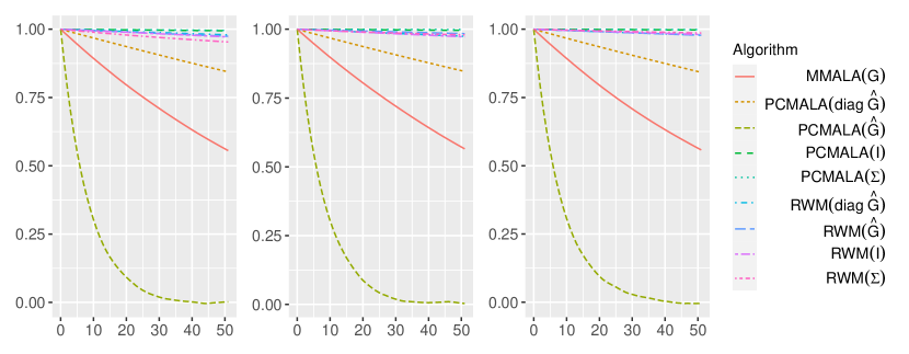
Figure 1: ACF plots for $x^{(1)}$ (left panel), $x^{(175)}$ (center panel), and $x^{(350)}$ (right panel) for the MH chains for the binomial SGLMM with the logit link. In the legend, $G$ refers to $\mathscr{I}^{-1}$ and $\hat{G}$ refers to $\hat{\mathscr{I}}^{-1}$.

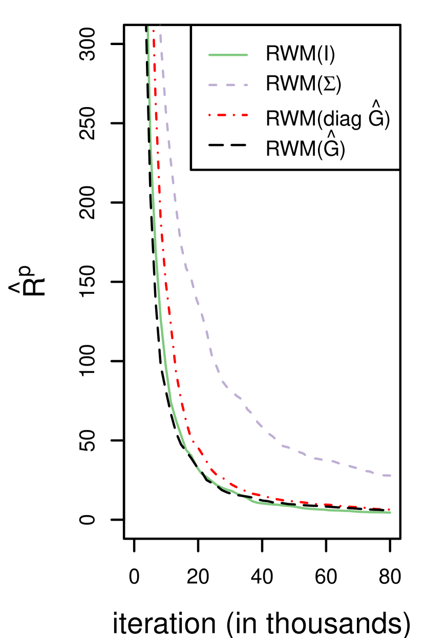
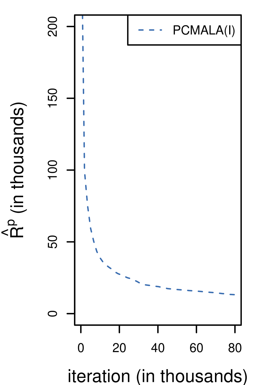
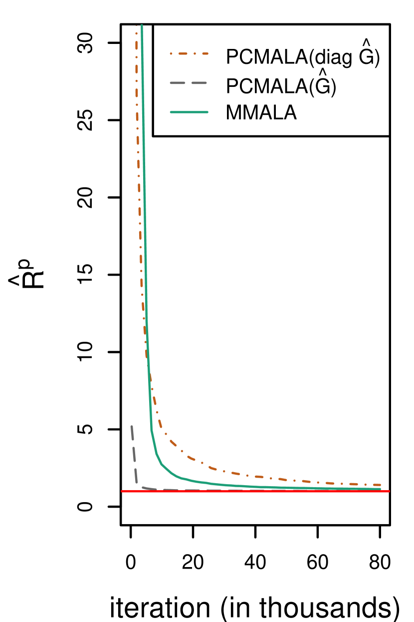
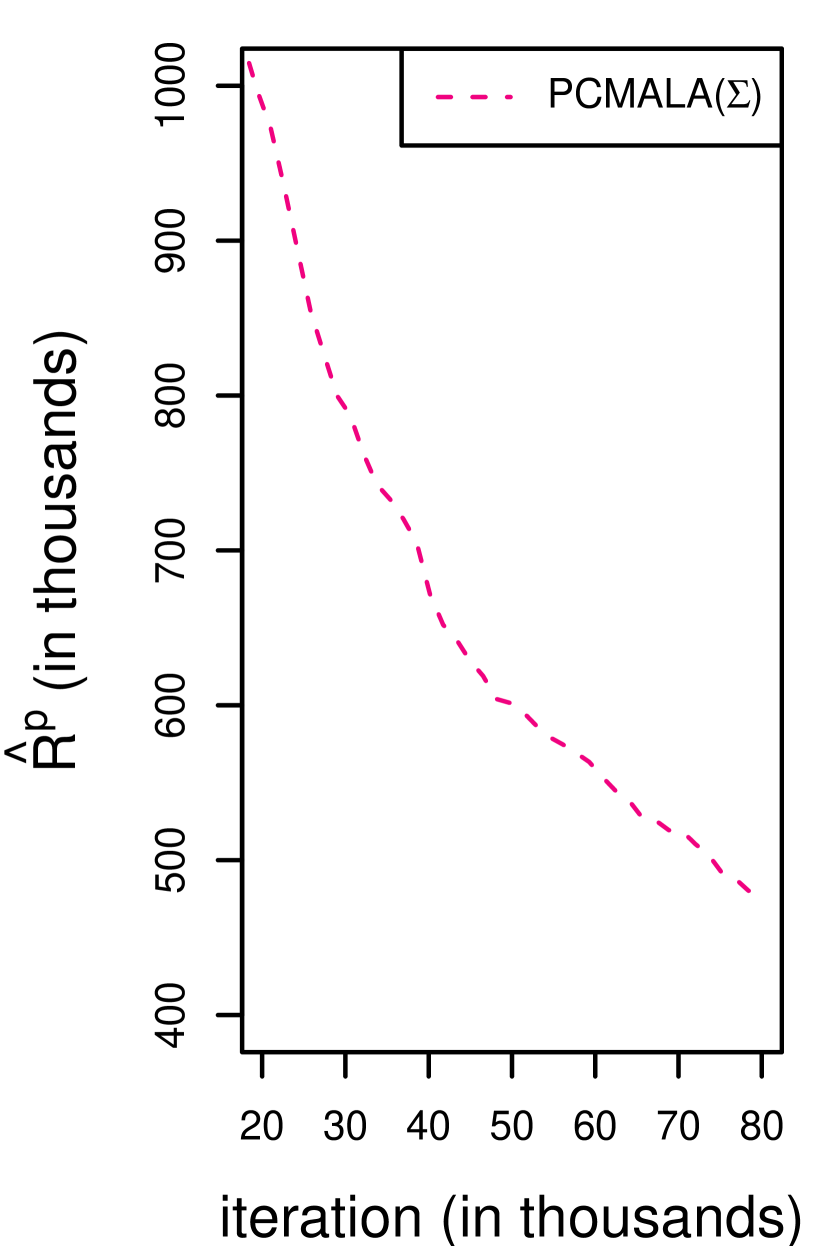
Figure 2: Gelman and Rubin’s $\hat{R}_{p}$ plot from the five parallel MH chains for the binomial SGLMM with the logit link. The red horizontal line on the third plot from the left has unit height. In the legend, $G$ refers to $\mathscr{I}^{-1}$ and $\hat{G}$ refers to $\hat{\mathscr{I}}^{-1}$.

6.3 Comparison of the pre-conditioned unadjusted Langevin algorithms

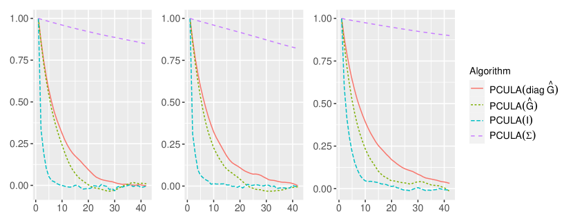
Figure S3: ACF plots for $x^{(1)}$ (left panel), $x^{(175)}$ (center panel), and $x^{(350)}$ (right panel) for the PCULA chains for the binomial SGLMM with the logit link. In the legend, $\hat{G}$ refers to $\hat{\mathscr{I}}^{-1}$.

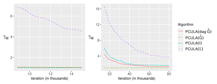
Figure S5: Gelman and Rubin’s $\hat{R}_{p}$ plot from the five parallel PCULA chains for the binomial-logit (left) and the Poisson-log SGLMMs (right). In the legend, $\hat{G}$ refers to $\hat{\mathscr{I}}^{-1}$.

In this section, we compare the four PCULA chains mentioned before in the context of simulated data from the binomial and Poisson SGLMMs. Since the unique stationary density of each of these PCULA is different, we do not use ESS for comparing these chains. As in Section 6.2, we ran each of the PCULA chains for 150,000 iterations starting at $x_{\text{true}}$. Table S3 provides the MSJD values for the PCULA chains for the binomial and the Poisson SGLMMs. As for the PCMALA, we see that when the pre-conditioning matrix $G$ is $\hat{\mathscr{I}}^{-1}$, the PCULA chain results in higher mixing than the other PCULA chains. Figures S3 and S4 provide the ACF values for the first 50 lags. For the binomial model, we see that except when $G=\Sigma$, for the other PCULA chains, the ACF values drop down quickly. Also, for the binomial SGLMM, for smaller lags, PCULA4 has slightly higher ACF values than PCULA1 ($G=I$). Recall that, if $G=I$, the PCULA boils down to the ULA. For the Poisson SGLMM, for PCULA4, the ACF values (practically) drop down to zero before five lags, whereas, the ACF values for the other three PCULA are quite large even after 50 lags. Thus, as for the adjusted Langevin algorithms, the pre-conditioning matrix $\hat{\mathscr{I}}^{-1}$ results in better PCULA than the other choices of $G$ considered here. Finally, Figure S5 provides the $\hat{R}_{p}$ plots based on the five Markov chains started at the same five points $x_{\text{true}}$, $-x_{\text{true}}$, $0$ and $x_{\text{true}}\pm 1$ as in Section 6.2, for each of the four PCULA chains. For both binomial and Poisson SGLMMs, the $\hat{R}_{p}$ reaches below 1.1 before 5,000 iterations of the PCULA4 chain. The PCULA3 algorithm ($G=\text{diag}(\hat{\mathscr{I}}^{-1})$) is the second best performer in terms of $\hat{R}_{p}$.

7 Discussions

In this paper, we establish conditions for geometric convergence of general MH algorithms with normal proposal density involving a position-dependent covariance matrix. If the mean of the proposal distribution is of the form $x+he(x)$, where $x$ denotes the current state, the users implementing these MCMC algorithms should make sure that $\|e(x)\|$ does not grow too fast with $\|x\|$. Similarly, if $\|e(x)\|$ shrinks, then the tails of $f(x)$ need to die down rapidly. As special cases, our results apply to the MMALA and other modern variants of the MALA. For the MMALA and other MALA chains, first and higher-order derivatives of the log target density are required. Here, in our GLMM examples, the derivatives are available in closed form. Girolami and Calderhead (2011) discuss several alternatives of the expected Fisher information matrix when it is not analytically available (see also Section 4.4 of Livingstone and Girolami, 2014). In the numerical examples involving binomial and Poisson SGLMMs, we observe that the PCMALA with an appropriate pre-conditioning matrix performs favorably than the advanced MMALA. Thus, in practice, it is worthwhile to construct suitable PCMALA chains that may have superior performance than the modern computationally expensive versions of MALA like the MMALA chain. On the other hand, MMALA may dominate the PCMALA with the pre-conditioning matrices used here for heavy-tailed distributions or targets with a fast changing Hessian, for example, the perturbed Gaussian density of Chewi et al. (2021) or the Example 4 of Gorham et al. (2019) (see also Taylor, 2015; Latuszynski et al., 2011).

Here, we have not considered a quantitative bound for the total variation norm (7), although with some modification of our results such bounds can be obtained. For example, Rosenthal (1995) use the method of coupling along with the drift and minorization technique to construct such quantitative bounds. On the other hand, these bounds are often too conservative to be used in practice (Qin and Hobert, 2021). Recently, Durmus and Moulines (2015) and Durmus and Moulines (2019) build some quantitative bounds for certain MALA and ULA chains. We believe that our results are a useful pre-cursor to constructing sharper quantitative bounds for position dependent MALA chains.

As mentioned before, Livingstone et al. (2019) establish geometric ergodicity of the HMC when the ‘mass matrix’ in the ‘kinetic energy’ is fixed (see also Mangoubi and Smith, 2021). On the other hand, Girolami and Calderhead (2011) argue that a position-dependent mass matrix in the HMC may be preferred, and they develop the Riemann manifold HMC (RMHMC). The techniques of this paper can be extended to establish convergence results of the RMHMC algorithms and we plan to undertake this as a future study. Finally, Langevin methods have been applied to several Bayesian models (see e.g. Møller et al., 1998; Girolami and Calderhead, 2011; Neal, 2012). It would be interesting to compare the performance of the PMALA and the PCMALA in the context of these examples.

Supplement to
“Convergence of position-dependent MALA with application to conditional simulation in GLMMs”
Vivekananda Roy and Lijin Zhang

S1 Proofs of results

Proof of Theorem 1.

From the form of (14), and by A2, we know that $P$ is $\phi$-irreducible and aperiodic. Let $C$ be a nonempty compact set. Since $f$ is bounded away from $0$ and $\infty$ on compact sets and A1 and A2 are in force, we have $\varepsilon=\inf_{x,y\in C}q(x,y)>0$ and $u=\sup_{x\in C}f(x)<\infty$. Let $B\subseteq C$. Then for any $x\in C$

$$P(x,B) \geq\int_{A(x)\cap B}q(x,y)\alpha(x,y)dy+\int_{R(x)\cap B}q(x,y)\alpha(x,y)dy$$

$$=\int_{A(x)\cap B}q(x,y)dy+\int_{R(x)\cap B}\frac{f(y)}{f(x)}q(y,x)dy$$

$$\geq\varepsilon\int_{A(x)\cap B}\frac{f(y)}{u}dy+\frac{\varepsilon}{u}\int_{R(x)\cap B}f(y)dy=\frac{\varepsilon}{u}F(B).$$

Thus, $C$ is small. Let $V_{s}(x)=\exp\{s\|G_{2}^{-1/2}x\|\}$, with $s>0$. We will show that with this drift function, Proposition 2 holds, implying geometric ergodicity of the MH chain. From (10) and (11), we have

$$PV_{s}(x)=\int_{R^{d}}q(x,y)\alpha(x,y)V_{s}(y)dy+V_{s}(x)\int_{R(x)}q(x,y)(1-\alpha(x,y))dy,$$

implying

$$\frac{PV_{s}(x)}{V_{s}(x)}\leq\int_{R^{d}}q(x,y)\frac{V_{s}(y)}{V_{s}(x)}dy+\int_{R(x)}q(x,y)(1-\alpha(x,y))dy.$$ (S1)

Since $V_{s}(x)=\exp\{s\|G_{2}^{-1/2}x\|\}$, by A1, the first term in the right side of (S1) is as large as

$$(2\pi h)^{-d/2}|G_{1}|^{-1/2}\int_{R^{d}}\exp\Big{\{}-\frac{1}{2h}(y-c(x))^{\top}G_{2}^{-1}(y-c(x))+s(\|G_{2}^{-1/2}y\|-\|G_{2}^{-1/2}x\|)\Big{\}}dy.$$ (S2)

Since $\|G_{2}^{-1/2}y\|\leq\|G_{2}^{-1/2}(y-c(x))\|+\|G_{2}^{-1/2}c(x)\|$, letting $z=G_{2}^{-1/2}(y-c(x))$, from (S2), it follows that the first term in the right side of (S1) is as large as

$$\frac{\exp\{-s(\|G_{2}^{-1/2}x\|-\|G_{2}^{-1/2}c(x)\|-sh/2)\}}{(2\pi h)^{d/2}|G_{1}|^{1/2}|G_{2}|^{-1/2}}\int_{R^{d}}\exp\big{\{}-[\|z\|^{2}-2sh\|z\|+s^{2}h^{2}]/2h\big{\}}dz.$$ (S3)

Now, we consider the polar transformation $(z_{1},\dots,z_{d})\rightarrow(r,\theta_{1},\theta_{2},\dots,\theta_{d-1})$ such that $z_{1}=r\cos\theta_{1},z_{2}=r\sin\theta_{1}\cos\theta_{2},\dots,z_{d-1}=r\sin\theta_{1}\dots\sin\theta_{d-2}\cos\theta_{d-1},z_{d}=r\sin\theta_{1}\dots\sin\theta_{d-2}\sin\theta_{d-1}$. Here, $r>0,0<\theta_{d-1}<2\pi$, $0<\theta_{i}<\pi,i=1,\dots,d-2$, and the Jacobian is $r^{d-1}\prod_{i=1}^{d-2}\sin^{d-1-i}\theta_{i}$. Thus,

$$\int_{R^{d}}\exp\Bigg{\{}-\frac{\|z\|^{2}-2sh\|z\|+s^{2}h^{2}}{2h}\Bigg{\}}dz \leq\int_{0}^{2\pi}\int_{0}^{\pi}\dots\int_{0}^{\pi}\int_{0}^{\infty}\exp\Bigg{\{}\frac{-(r-hs)^{2}}{2h}\Bigg{\}}r^{d-1}drd\theta_{1}\dots d\theta_{d-2}d\theta_{d-1}$$

$$=2\pi^{d-1}\int_{0}^{\infty}\exp\{-(r-hs)^{2}/(2h)\}r^{d-1}dr.$$ (S4)

Using (S3) and (S1), from (S1) we have

$$\limsup_{\|x\|\rightarrow\infty}\frac{PV_{s}(x)}{V_{s}(x)}\leq C_{2}(s)\exp(-s\eta)+C_{1}.$$ (S5)

Thus under A4, (12) holds. Also, from (S1)–(S1) by A2 we have

$$\sup_{\|x\|\leq k}\frac{PV_{s}(x)}{V_{s}(x)}\leq 1+C_{2}(s)\sup_{\|x\|\leq k}\exp\{s(\|G_{2}^{-1/2}c(x)\|-\|G_{2}^{-1/2}x\|)\}<\infty.$$

Hence, the proof follows from Proposition 2. ∎

Proof of Theorem 2.

As in the proof of Theorem 1, we know that $P$ is $\phi$-irreducible, aperiodic, and nonempty compact sets are small. Let $V(x)=x^{\top}x$. Then,

$$\int_{R^{d}}\frac{V(y)}{V(x)}q(x,y)dy \leq\frac{1}{x^{\top}x}(2\pi h)^{-d/2}|G_{1}|^{-1/2}\int_{R^{d}}\big{[}y^{\top}y\big{]}\exp\Big{\{}-\frac{1}{2h}(y-c(x))^{\top}G_{2}^{-1}(y-c(x))\Big{\}}dy$$

$$=\frac{c(x)^{\top}c(x)+tr(hG_{2})}{x^{\top}x}(|G_{2}|/|G_{1}|)^{1/2}.$$ (S6)

Thus, from (S1) and (S1) we have

$$\limsup_{\|x\|\rightarrow\infty}\frac{PV(x)}{V(x)}\leq\Big{(}\frac{|G_{2}|}{|G_{1}|}\Big{)}^{1/2}\limsup_{\|x\|\rightarrow\infty}\frac{\|c(x)\|^{2}}{\|x\|^{2}}+C_{1}.$$ (S7)

Also, note that by A2 we have

$$\sup_{\|x\|\leq k}PV(x)\leq k^{2}+(|G_{2}|/|G_{1}|)^{1/2}\sup_{\|x\|\leq k}\Big{[}c(x)^{\top}c(x)+tr(hG_{2})\Big{]}<\infty.$$

Hence, the proof follows by (S7) and applying Proposition 2 on the function $V(x)+1$ as A5 is in force. ∎

Proof of Theorem 3.

Since $c(x)=x+he(x)$, from (14) we have

$$Q(x,B_{k}(x))\geq(2\pi h)^{-d/2}|G_{2}|^{-1/2}\int_{\|z\|<k}\exp\Big{\{}-\frac{1}{2h}(z-he(x))^{\top}G_{1}^{-1}(z-he(x))\Big{\}}dz.$$ (S8)

Then, by $\|e(x)\|<M$ it follows that for given $\varepsilon>0$, there exists $k$ such that $Q(x,B_{k}(x))>1-\varepsilon$. Thus, the result follows from Proposition 3. ∎

Proof of Theorem 4.

Choose $T>2/h$, such that when $S_{1}$ is large enough,

$$\inf_{\|x\|>S_{1}}\frac{\|e(x)\|}{\|x\|}>T.$$

Define $B^{2}_{k}(x)=\{y:\|y-c(x)\|\leq k\}$. By A1, for given $\varepsilon>0$, there exists $k_{\varepsilon}$, such that $\int_{R^{d}/B^{2}_{k_{\varepsilon}}(x)}q(x,y)dy<\varepsilon/2$. To simplify notations, for the rest of this proof, we denote $B^{2}_{k_{\varepsilon}}(x)$ by $B^{2}_{\varepsilon}(x)$. When $y\in B^{2}_{\varepsilon}(x)$, $q(x,y)$ is bounded away from 0, as

$$q(x,y)\geq(2\pi h\zeta_{2}^{+})^{-d/2}\exp\{-k_{\varepsilon}^{2}/[2h\zeta_{1+}]\}.$$ (S9)

Note that, the proposed $y$ is generated as $y=x+he(x)+\sqrt{hG(x)}\epsilon$, which is either accepted or rejected with the chain staying at the current position $x$. Here $\epsilon\sim N(0,I_{d})$. Since,

$$\|y\|=\|x+he(x)+\sqrt{hG(x)}\epsilon\|\geq h\|e(x)\|-\|x\|-\sqrt{h}\|\sqrt{G(x)}\epsilon\|,$$

we have

$$\frac{\|y\|}{\|x\|}\geq h\frac{\|e(x)\|}{\|x\|}-1-\sqrt{h}\frac{\|\sqrt{G(x)}\epsilon\|}{\|x\|}.$$

Hence, by (17), $\exists\;S_{2}$ such that when $\|x\|>S_{2}$ and $y\in B^{2}_{\varepsilon}(x)$, we have $\|y\|>\|x\|$. Let $S=$ max $(S_{1},S_{2})$. Thus, when $y\in B_{\varepsilon}(x)$, and $\|x\|>S$,

$$\|he(y)\|>hT\|y\|>2\|y\|>\|x\|+\|y\|>\|x-y\|,$$

and hence,

$$\|x-y-he(y)\|\geq\|he(y)\|-\|x-y\|\geq hT\|y\|-2\|y\|.$$

So, for $y\in B_{\varepsilon}(x)$, and $\|x\|>S$, we have

$$q(y,x) \leq(2\pi h\zeta_{1+})^{-d/2}\exp\big{\{}-\frac{1}{2h\zeta_{2}^{+}}\|x-y-he(y)\|^{2}\big{\}}$$

$$\leq(2\pi h\zeta_{1+})^{-d/2}\exp\{-(hT-2)^{2}\|y\|^{2}/[2h\zeta_{2}^{+}]\},$$

and, thus when $\|x\|\rightarrow\infty$,

$$\sup_{y\in B^{2}_{\varepsilon}(x)}q(y,x)\leq(2\pi h\zeta_{1+})^{-d/2}\exp\{-(hT-2)^{2}\|x\|^{2}/[2h\zeta_{2}^{+}]\}\rightarrow 0.$$ (S10)

From (S9) and (S10) we have

$$\sup_{y\in B^{2}_{\varepsilon}(x)}\frac{q(y,x)}{q(x,y)}\leq\frac{\sup_{y\in B^{2}_{\varepsilon}(x)}q(y,x)}{\inf_{y\in B^{2}_{\varepsilon}(x)}q(x,y)}\rightarrow 0\;\text{as}\;\|x\|\rightarrow\infty.$$ (S11)

Starting with $\|x_{0}\|>S$ and $f(x_{0})>0$, define $x_{n}=\text{arg}\sup\{f(y);y\in B^{2}_{\varepsilon}(x_{n-1})\}$. Note that $\|x_{n}\|\rightarrow\infty$ when $n\rightarrow\infty$. Assume that the MH chain is GE, then, from Section 3 there exists $\varepsilon>0$, such that $\text{ess}\sup r(x)<1-\varepsilon$. Now,

$$\text{ess}\sup r(x_{n}) =\text{ess}\sup\big{\{}1-\int_{R^{d}}\alpha(x_{n},y)q(x_{n},y)dy\big{\}}$$

$$\geq 1-\text{ess}\sup\big{\{}\int_{R^{d}}\alpha(x_{n},y)q(x_{n},y)dy\big{\}}.$$

Thus,

$$1-\text{ess}\sup r(x_{n})\leq\sup\int_{R^{d}}\alpha(x_{n},y)q(x_{n},y)dy,$$

and with the fact that $\int_{R^{d}/B^{2}_{\varepsilon}(x_{n})}q(x_{n},y)dy\leq\varepsilon/2$, we have

$$1-\text{ess}\sup r(x_{n}) \leq\sup\int_{R^{d}/B^{2}_{\varepsilon}(x_{n})}\Big{\{}1\wedge\frac{f(y)}{f(x_{n})}\frac{q(y,x_{n})}{q(x_{n},y)}\Big{\}}q(x_{n},y)dy$$

$$+\sup\int_{B^{2}_{\varepsilon}(x_{n})}\Big{\{}1\wedge\frac{f(y)}{f(x_{n})}\frac{q(y,x_{n})}{q(x_{n},y)}\Big{\}}q(x_{n},y)dy$$

$$\leq\sup\int_{R^{d}/B^{2}_{\varepsilon}(x_{n})}q(x_{n},y)\mu(dy)+\sup\int_{B^{2}_{\varepsilon}(x_{n})}\Big{\{}1\wedge\frac{f(y)}{f(x_{n})}\frac{q(y,x_{n})}{q(x_{n},y)}\Big{\}}q(x_{n},y)dy$$

$$\leq\frac{\varepsilon}{2}+\sup\int_{B^{2}_{\varepsilon}(x_{n})}1\wedge\frac{f(y)}{f(x_{n})}\frac{q(y,x_{n})}{q(x_{n},y)}q(x_{n},y)dy.$$

Thus,

$$\varepsilon< 1-\text{ess}\sup r(x_{n})\leq\frac{\varepsilon}{2}+\sup\int_{B^{2}_{\varepsilon}(x_{n})}\Big{\{}1\wedge\frac{f(y)}{f(x_{n})}\frac{q(y,x_{n})}{q(x_{n},y)}\Big{\}}q(x_{n},y)dy$$

$$\Rightarrow\sup\int_{B^{2}_{\varepsilon}(x_{n})}\Big{\{}1\wedge\frac{f(y)}{f(x_{n})}\frac{q(y,x_{n})}{q(x_{n},y)}\Big{\}}q(x_{n},y)\mu(dy)>\frac{\varepsilon}{2}.$$ (S12)

From (S11), when $n>N$ and $N$ is large enough, we have $\sup_{y\in B^{2}_{\varepsilon}(x_{n})}[q(y,x_{n})/q(x_{n},y)]<\varepsilon/4$. Thus from (S1) we have

$$\frac{\varepsilon}{2}\leq\sup\int_{B^{2}_{\varepsilon}(x_{n})}\Big{\{}1\wedge\frac{\varepsilon}{4}\frac{f(x_{n+1})}{f(x_{n})}\Big{\}}q(x_{n},y)dy\leq\frac{\varepsilon}{4}\frac{f(x_{n+1})}{f(x_{n})},$$

implying $f(x_{n+1})>2f(x_{n})$, which contradicts that $f$ is bounded. Therefore, the MH chain is not geometric ergodic. ∎

Proof of Proposition 4.

Since $c(x)$ is continuous, by Fatou’s lemma for a fixed open set $A\in\mathbb{R}^{d}$,

$$\liminf_{x_{n}\rightarrow x}Q(x_{n},A)=\liminf_{x_{n}\rightarrow x}\frac{|G|^{-1/2}}{(2\pi h)^{d/2}}\int_{A}\exp\Big{\{}-\frac{1}{2h}(y-c(x_{n}))^{\top}G^{-1}(y-c(x_{n}))\Big{\}}dy\geq Q(x,A).$$

Thus, $\{X_{n}\}_{n\geq 0}$ is a Feller chain. From the proof of Theorem 1, we have

$$\limsup_{\|x\|\rightarrow\infty}\frac{QV_{s}(x)}{V_{s}(x)}<1,$$

and as $V_{s}$ is unbounded off compact sets, by Proposition 1, $\{X_{n}\}_{n\geq 0}$ is GE when A4 holds. Similarly, the proof for A5 follows by Proposition 1, and using the drift function $V$ from Theorem 2. ∎

Proof of Theorem 5.

For the PCMALA chain A1 holds automatically. Recall that the proposal density for PCMALA is $N(x+hG\nabla\log f(x)/2,hG)$. Thus, from (23) it follows that the proposal density for the PCMALA is (14) with $G(x)=G$ and

$$c(x)=x+(h/2)G(-\Sigma^{-1}x+b(x)),$$ (S13)

where $b(x)=z-\ell\cdot(e^{x}/[1+e^{x}])+\Sigma^{-1}D\beta$ is bounded. Thus, A2 holds for the PCMALA chain. We now show that A3 holds for the PCMALA chain. For a given $0<\varepsilon<1$, set $B_{\varepsilon}^{3}(x)=\{y:\|G^{-1/2}(y-c(x))\|<k_{\varepsilon}\}$, and $k_{\varepsilon}>0$, such that $\int_{R^{m}\setminus B_{\varepsilon}^{3}(x)}q(x,y)dy<\varepsilon$.

From (22) the acceptance probability $\alpha(x,y)$ in (2) becomes

$$1\wedge\exp\{-\log q(x,y)+\log q(y,x)+\log p(y)-\log p(x)+\sum_{i=1}^{m}\log a(z_{i},\mu_{i}(y))-\sum_{i=1}^{m}\log a(z_{i},\mu_{i}(x))\}.$$

We will show that the proposal $y\in B_{\varepsilon}^{3}(x)$ is always accepted when $\|x\|\rightarrow\infty$. From (14) and (S13) for the PCMALA we have

$$-\log q(x,y)-m\log(2h\pi)/2-\log|G|/2$$

$$= \frac{1}{2h}\Big{(}y-x-\frac{h}{2}G(-\Sigma^{-1}x+b(x))\Big{)}^{\top}G^{-1}\Big{(}y-x-\frac{h}{2}G(-\Sigma^{-1}x+b(x))\Big{)}$$

$$= \frac{1}{2h}y^{\top}G^{-1}y+\frac{1}{2h}x^{\top}G^{-1}x+\frac{h}{8}x^{\top}\Sigma^{-1}G\Sigma^{-1}x+\frac{h}{8}b(x)^{\top}Gb(x)$$

$$-\frac{1}{h}y^{\top}G^{-1}x+\frac{1}{2}y^{\top}\Sigma^{-1}x-\frac{1}{2}y^{\top}b(x)-\frac{1}{2}x^{\top}\Sigma^{-1}x+\frac{1}{2}x^{\top}b(x)-\frac{h}{4}x^{\top}\Sigma^{-1}Gb(x).$$

Let

$$L_{1} =\frac{h}{8}(x^{\top}\Sigma^{-1}G\Sigma^{-1}x-y^{\top}\Sigma^{-1}G\Sigma^{-1}y),$$

$$L_{2} =\frac{h}{8}(b(x)^{\top}Gb(x)-b(y)^{\top}Gb(y)),$$

$$L_{3} =\frac{1}{2}x^{\top}(I-h\Sigma^{-1}G/2)b(x)-\frac{1}{2}y^{\top}(I-h\Sigma^{-1}G/2)b(y)+\frac{1}{2}x^{\top}b(y)-\frac{1}{2}y^{\top}b(x),\;\text{and}$$

$$L_{4} =\log p(y)-\log p(x)+\sum_{i=1}^{m}\log a(z_{i},\mu_{i}(y))-\sum_{i=1}^{m}\log a(z_{i},\mu_{i}(x))-\frac{1}{2}x^{\top}\Sigma^{-1}x+\frac{1}{2}y^{\top}\Sigma^{-1}y.$$ (S14)

Note that $\alpha(x,y)=1\wedge\exp\{L_{1}+L_{2}+L_{3}+L_{4}\}$. If $L_{1}+L_{2}+L_{3}+L_{4}\geq 0$, then the proposed $y$ would always be accepted. Again, from (S13), for $y\in B_{\varepsilon}^{3}(x)$, we have

$$y^{\top}\Sigma^{-1}G\Sigma^{-1}y =\big{(}\big{(}I-\frac{h}{2}G\Sigma^{-1}\big{)}x+O(1)\big{)}^{\top}\Sigma^{-1}G\Sigma^{-1}\big{(}\big{(}I-\frac{h}{2}G\Sigma^{-1}\big{)}x+O(1)\big{)}$$

$$=x^{\top}\Sigma^{-1}G\Sigma^{-1}x+\frac{h^{2}}{4}x^{\top}\Sigma^{-1}G\Sigma^{-1}G\Sigma^{-1}G\Sigma^{-1}x+O(1)^{\top}\Sigma^{-1}G\Sigma^{-1}O(1)$$

$$-hx^{\top}\Sigma^{-1}G\Sigma^{-1}G\Sigma^{-1}x+2x^{\top}\Sigma^{-1}G\Sigma^{-1}O(1)-hx^{\top}\Sigma^{-1}G\Sigma^{-1}G\Sigma^{-1}O(1).$$ (S15)

Let $\psi_{+}(\zeta_{+})$ and $\psi^{+}(\zeta^{+})$ be the smallest and the largest eigenvalue of $\Sigma^{-1}(G)$, respectively. Note that, $x^{\top}\Sigma^{-1}G\Sigma^{-1}x/\|x\|^{2}\in[\psi_{+}^{2}\zeta_{+},\psi^{+2}\zeta^{+}]$. Similarly $x^{\top}\Sigma^{-1}G\Sigma^{-1}G\Sigma^{-1}x/\|x\|^{2}\in[\psi_{+}^{3}\zeta_{+}^{2},\psi^{+3}\zeta^{+2}],$ and $x^{\top}\Sigma^{-1}G\Sigma^{-1}G\Sigma^{-1}G\Sigma^{-1}x/\|x\|^{2}\in[\psi_{+}^{4}\zeta_{+}^{3},\psi^{+4}\zeta^{+3}]$. Thus, from (S1) and (S1) we have

$$L_{1}= \frac{h}{8}\big{(}-\frac{h^{2}}{4}x^{\top}\Sigma^{-1}G\Sigma^{-1}G\Sigma^{-1}x-O(1)^{\top}\Sigma^{-1}O(1)+hx^{\top}\Sigma^{-1}G\Sigma^{-1}x-2x^{\top}\Sigma^{-1}O(1)$$

$$+hx^{\top}\Sigma^{-1}G\Sigma^{-1}O(1)\big{)}$$

$$\geq -\frac{h^{3}}{32}\psi^{+3}\zeta^{+2}\|x\|^{2}+\frac{h^{2}}{8}\psi_{+}^{2}\zeta_{+}\|x\|^{2}+o(\|x\|^{2}).$$

So, if $h\in(0,4\psi_{+}^{2}\zeta_{+}/[\psi^{+3}\zeta^{+2}]),$ when $\|x\|\rightarrow\infty$, $L_{1}\rightarrow\infty$. Also, note that for such $h,$ $L_{1}\sim\|x\|^{2}$, $L_{2}$ is bounded and $L_{3}=o(L_{1})$. Here, $i(x)\sim j(x)$ means $i(x)/j(x)\rightarrow c$ for some constant $c>0$. Since $\lim_{t\rightarrow-\infty}\log(1+\exp{[t]})/t^{2}=0$ and by L’Hospital’s rule, $\lim_{t\rightarrow\infty}\log(1+\exp{[t]})/t^{2}=0$, we have

$$L_{4}= \log p(y)-\log p(x)+\sum_{i=1}^{m}\log a(z_{i},\mu_{i}(y))-\sum_{i=1}^{m}\log a(z_{i},\mu_{i}(x))-\frac{1}{2}x^{\top}\Sigma^{-1}x+\frac{1}{2}y^{\top}\Sigma^{-1}y$$

$$= -\frac{1}{2}(y-D\beta)^{\top}\Sigma^{-1}(y-D\beta)+\sum_{i=1}^{m}\{z_{i}y^{(i)}-\ell_{i}\log(1+\exp(y^{(i)}))\}+$$

$$\frac{1}{2}(x-D\beta)^{\top}\Sigma^{-1}(x-D\beta)-\sum_{i=1}^{m}\{z_{i}x^{(i)}-\ell_{i}\log(1+\exp(x^{(i)}))\}-\frac{1}{2}x^{\top}\Sigma^{-1}x+\frac{1}{2}y^{\top}\Sigma^{-1}y$$

$$= o(\|x\|^{2}).$$

Therefore, for large $\|x\|$, $B_{\varepsilon}^{3}(x)\subseteq A(x)$. Recall that, $A(x)=\{y:f(x)q(x,y)\leq f(y)q(y,x)\}=R(x)^{c}$. Thus,

$$\liminf_{\|x\|\rightarrow\infty}\int_{A(x)}q(x,y)dy \geq\liminf_{\|x\|\rightarrow\infty}\int_{B_{\varepsilon}^{3}(x)}q(x,y)dy>1-\varepsilon>0.$$

Hence,

$$C_{1}=\limsup_{\|x\|\rightarrow\infty}\int_{R(x)}q(x,y)(1-\alpha(x,y))dy \leq\limsup_{\|x\|\rightarrow\infty}\int_{R(x)}q(x,y)dy$$

$$\leq 1-\liminf_{\|x\|\rightarrow\infty}\int_{A(x)}q(x,y)dy<1.$$

Thus, A3 holds for the PCMALA chain. Next, we verify A4. From (S13), note that

$$\|x\|-\|c(x)\| =\|x\|-\|(I-(h/2)G\Sigma^{-1})x+(h/2)Gb(x)\|$$

$$\geq\|x\|-\|(I-(h/2)G\Sigma^{-1})x\|-\|(h/2)Gb(x)\|.$$ (S16)

Now, if $1-h\psi_{+}\zeta_{+}+h^{2}\psi^{+2}\zeta^{+2}/4<1\Leftrightarrow h<4\psi_{+}\zeta_{+}/\psi^{+2}\zeta^{+2}$, then $\|(I-(h/2)G\Sigma^{-1})x\|^{2}/x^{\top}x<1$. Since $b(x)$ is bounded, and $\psi_{+}/\psi^{+}<1$, if $h\in(0,4\psi_{+}^{2}\zeta_{+}/(\psi^{+3}\zeta^{+2}))$, from (S1), we have $\liminf_{\|x\|\rightarrow\infty}\big{(}\|x\|-\|c(x)\|\big{)}=\infty$. Thus, by Remark 2, it follows that A4 holds for the PCMALA chain. Thus for $h\in(0,4\psi_{+}^{2}\zeta_{+}/(\psi^{+3}\zeta^{+2}))$ geometric ergodicity of the PCMALA chain follows from Theorem 1.

Next, we verify A1–A4 for the MMALA chain. Since

$$G_{1}\equiv(0.25\text{diag}(\ell)+\Sigma^{-1})^{-1}\leq\mathscr{I}^{-1}(x)\leq\Sigma\equiv G_{2},$$ (S17)

A1 holds for the MMALA. The mean of the proposal distribution for the MMALA is $c(x)=x+(h/2)\mathscr{I}^{-1}(x)\nabla\log f(x)+(h/2)\Gamma(x)$ where $\Gamma(x)$ is given in (25). Thus,

$$c(x)=x+(h/2)\mathscr{I}^{-1}(x)(-\Sigma^{-1}x+\kappa(x)),$$ (S18)

where $\kappa(x)=b(x)+\mathscr{I}(x)\Gamma(x)$. From (24) it follows that $(\partial\mathscr{I}_{jj}(x)/\partial x_{j})$ is bounded. By (S17) we have $\mathscr{I}^{-1}_{jj}(x)$ is bounded for all $j$, and then, an application of the Cauchy-Schwartz inequality shows that $\mathscr{I}^{-1}_{ij}(x)$ is bounded. Thus, from (25) it follows that $\kappa(x)$ is bounded, and A2 holds for the MMALA chain.

Note that,

$$-\log q(x,y)-m\log(2h\pi)/2+\log|\mathscr{I}(x)|/2$$

$$= \frac{1}{2h}\big{(}y-x-\frac{h}{2}\big{\{}\mathscr{I}^{-1}(x)(-\Sigma^{-1}x+\kappa(x))\big{\}}\big{)}^{\top}\mathscr{I}(x)\big{(}y-x-\frac{h}{2}\big{\{}\mathscr{I}^{-1}(x)(-\Sigma^{-1}x+\kappa(x))\big{\}}\big{)}$$

$$= \frac{1}{2h}y^{\top}\mathscr{I}(x)y+\frac{1}{2h}x^{\top}\mathscr{I}(x)x+\frac{h}{8}x^{\top}\Sigma^{-1}\mathscr{I}^{-1}(x)\Sigma^{-1}x+\frac{h}{8}\kappa(x)^{\top}\mathscr{I}^{-1}(x)\kappa(x)-\frac{1}{h}y^{\top}\mathscr{I}(x)x$$

$$+\frac{1}{2}y^{\top}\Sigma^{-1}x-\frac{1}{2}y^{\top}\kappa(x)-\frac{1}{2}x^{\top}\Sigma^{-1}x+\frac{1}{2}x^{\top}\kappa(x)-\frac{h}{4}x^{\top}\Sigma^{-1}\mathscr{I}^{-1}(x)\kappa(x).$$

Let

$$L^{\prime}_{1} =h(x^{\top}\Sigma^{-1}\mathscr{I}^{-1}(x)\Sigma^{-1}x-y^{\top}\Sigma^{-1}\mathscr{I}^{-1}(y)\Sigma^{-1}y)/8,$$

$$L^{\prime}_{2} =h(\kappa(x)^{\top}\mathscr{I}^{-1}(x)\kappa(x)-\kappa(y)^{\top}\mathscr{I}^{-1}(y)\kappa(y))/8+\log(|\mathscr{I}(y)|/|\mathscr{I}(x)|)/2,$$

$$L^{\prime}_{3} =\frac{1}{2}x^{\top}(I-(h/2)\Sigma^{-1}\mathscr{I}^{-1}(x))\kappa(x)-\frac{1}{2}y^{\top}(I-(h/2)\Sigma^{-1}\mathscr{I}^{-1}(y))\kappa(y)+\frac{1}{2}x^{\top}\kappa(y)-\frac{1}{2}y^{\top}\kappa(x),$$

$$L^{\prime}_{5} =([\{x^{\top}\mathscr{I}(x)x-x^{\top}\mathscr{I}(y)x\}+\{y^{\top}\mathscr{I}(x)y-y^{\top}\mathscr{I}(y)y\}]/2-[x^{\top}\mathscr{I}(x)y-x^{\top}\mathscr{I}(y)y])/h.$$

Note that $\alpha(x,y)=1\wedge\exp\{L^{\prime}_{1}+L^{\prime}_{2}+L^{\prime}_{3}+L_{4}+L^{\prime}_{5}\}$. Define, $B^{4}_{k}(x)\equiv\{y:\|y-c(x)\|\leq k\;\&\;\prod_{i=1}^{m}x^{(i)}(x^{(i)}-y^{(i)})>0\}$. We can find $\varepsilon>0$ and $k_{\varepsilon}$ such that $\int_{R^{m}/B^{4}_{k_{\varepsilon}}(x)}q(x,y)dy<\varepsilon$. Thus, from (S17) and (S18), for $y\in B_{\varepsilon}^{4}(x)$, we have

$$y^{\top}\Sigma^{-1}\mathscr{I}^{-1}(y)\Sigma^{-1}y$$ (S19)

$$= \big{(}\big{(}I-(h/2)\mathscr{I}^{-1}(x)\Sigma^{-1}\big{)}x+O(1)\big{)}^{\top}\Sigma^{-1}\mathscr{I}^{-1}(y)\Sigma^{-1}\big{(}\big{(}I-(h/2)\mathscr{I}^{-1}(x)\Sigma^{-1}\big{)}x+O(1)\big{)}$$

$$= x^{\top}\Sigma^{-1}\mathscr{I}^{-1}(y)\Sigma^{-1}x+(h^{2}/4)x^{\top}\Sigma^{-1}\mathscr{I}^{-1}(x)\Sigma^{-1}\mathscr{I}^{-1}(y)\Sigma^{-1}\mathscr{I}^{-1}(x)\Sigma^{-1}x$$

$$-hx^{\top}\Sigma^{-1}\mathscr{I}^{-1}(y)\Sigma^{-1}\mathscr{I}^{-1}(x)\Sigma^{-1}x+o(\|x\|^{2}).$$ (S20)

Let $\iota(x^{(i)})=e^{x^{(i)}}/(1+e^{x^{(i)}})$, $\omega(x^{(i)})=\{\iota(x^{(i)})-\iota^{2}(x^{(i)})\}$, and $E(x)=\mbox{diag}(\ell_{1}\omega(x^{(1)}),\dots,\\ \ell_{m}\omega(x^{(m)})).$ Note that $\omega^{\prime}(t)=\iota(t)-3\iota^{2}(t)+2\iota^{3}(t)=\iota(t)(1-\iota(t))(1-2\iota(t))\gtreqless 0\iff t\lesseqgtr 0$. That is, $\omega(t)$ is decreasing (increasing) on the positive (negative) half line. So, for $y\in B_{\varepsilon}^{4}(x)$, $E(y)\geq E(x)$, implying $\mathscr{I}^{-1}(x)=(E(x)+\Sigma^{-1})^{-1}\geq(E(y)+\Sigma^{-1})^{-1}=\mathscr{I}^{-1}(y)$. So, $x^{\top}\Sigma^{-1}\mathscr{I}^{-1}(x)\Sigma^{-1}x-x^{\top}\Sigma^{-1}\mathscr{I}^{-1}(y)\Sigma^{-1}x\geq 0$. Thus, from (S19) we have

$$L^{\prime}_{1}\geq \frac{h}{8}(-h^{2}x^{\top}\Sigma^{-1}\mathscr{I}^{-1}(x)\Sigma^{-1}\mathscr{I}^{-1}(y)\Sigma^{-1}\mathscr{I}^{-1}(x)\Sigma^{-1}x/4+hx^{\top}\Sigma^{-1}\mathscr{I}^{-1}(y)\Sigma^{-1}\mathscr{I}^{-1}(x)\Sigma^{-1}x)+o(\|x\|^{2})$$

$$\geq \frac{h}{8}(h\psi_{+}^{3}\zeta_{1+}^{2}\|x\|^{2}-h^{2}\psi^{+4}\zeta_{2}^{+3}\|x\|^{2}/4)+o(\|x\|^{2}).$$

Recall that, $\zeta_{i+}$ and $\zeta_{i}^{+}$ are the smallest and the largest eigenvalue of $G_{i}$, respectively for $i=1,2$. So, if $h\in(0,4\psi_{+}^{3}\zeta_{1+}^{2}/[\psi^{+4}\zeta_{2}^{+3}]),$ when $\|x\|\rightarrow\infty$, $L^{\prime}_{1}\rightarrow\infty$. Also, $L^{\prime}_{2}$ is bounded, and $L^{\prime}_{3}=o(L^{\prime}_{1})$. Next, we consider $L^{\prime}_{5}$. Note that $\mathscr{I}_{ij}(x)-\mathscr{I}_{ij}(y)=0$ for $i\neq j$. Thus,

$$x^{\top}\mathscr{I}(x)x-x^{\top}\mathscr{I}(y)x=\sum_{i=1}^{m}(\mathscr{I}_{ii}(x)-\mathscr{I}_{ii}(y))x^{(i)2}=\sum_{i=1}^{m}\ell_{i}[\omega(x^{(i)})-\omega(y^{(i)})]x^{(i)2},$$

and

$$L^{\prime}_{5}=\sum_{i=1}^{m}\ell_{i}[\omega(x^{(i)})-\omega(y^{(i)})](x^{(i)}-y^{(i)})^{2}/2.$$

By (S17) and (S18), as $y\in B_{\varepsilon}^{4}(x)$, for small $h$ we have $\sum_{i=1}^{m}(x^{(i)}-y^{(i)})^{2}=O(1)$. Since $\iota(t)\in(0,1)$, for $y\in B_{\varepsilon}^{4}(x)$ we have $L^{\prime}_{5}=O(1)$. Then, using similar arguments as in the proof of geometric ergodicity for the PCMALA chain, we can show that A3 holds for the MMALA chain. Finally, for the MMALA

$$\|x\|-\|c(x)\|\geq\|x\|-\|(I-(h/2)\mathscr{I}^{-1}(x)\Sigma^{-1})x\|-\|(h/2)\mathscr{I}^{-1}(x)\kappa(x)\|.$$

If $h<4\psi_{+}\zeta_{1+}/\psi^{+2}\zeta_{2}^{+2}$, then $\|(I-(h/2)\mathscr{I}^{-1}(x)\Sigma^{-1})x\|^{2}/x^{\top}x<1$. Since $\zeta_{1+}/\zeta_{2}^{+}<1$, if $h\in(0,4\psi_{+}^{3}\zeta_{1+}^{2}/[\psi^{+4}\zeta_{2}^{+3}]),$ then A4 holds for the MMALA chain. Thus geometric ergodicity of the MMALA follows from Theorem 1.

Next, we consider the PCULA chain. From (S13) we know that the PCULA chain is given by

$$X_{n}=(I-(h/2)G\Sigma^{-1})X_{n-1}+b(X_{n-1})+\sqrt{h}G^{1/2}\epsilon,$$

where $b(x)=z-\ell\cdot(e^{x}/[1+e^{x}])+\Sigma^{-1}D\beta$. So, if $h$ is chosen such that the singular values of $(I-(h/2)G\Sigma^{-1})$ are less than one, then geometric ergodicity of the PCULA follows from (20) and Remark 10. ∎

Proof of Proposition 5.

Since $\lim_{\|x\|\rightarrow\infty}\prod_{i=1}^{m}\exp\{z_{i}x^{(i)}\}\exp\{-\exp\{x^{(i)}\}\}=0,$ if $z_{i}>0\;\forall i$, and otherwise is bounded, it follows that the target density $f(x)$ is bounded. From (27) we have

$$\|\nabla\log f(x)\|=\|z-\exp\{x\}-\Sigma^{-1}(x-D\beta)\|\geq\|\exp\{x\}\|-\|z\|-\|\Sigma^{-1}(x-D\beta)\|.$$ (S21)

Next, for $x^{(i)}>0,i=1,\dots,m$, from (S21) we have

$$\liminf_{\|x\|\rightarrow\infty}\|G\nabla\log f(x)\|/\|x\| \geq\liminf_{\|x\|\rightarrow\infty}\zeta_{+}\{1-(\|z\|+\|\Sigma^{-1}(x-D\beta)\|)/\|\exp\{x\}\|\}\|\exp\{x\}\|/\|x\|$$

$$=\infty.$$

Hence, the result follows from Theorem 4. ∎

S2 Additional numerical results for the SGLMMs

In this section, we include some tables and figures from the analysis of simulated data from the SGLMMs.

Table S1: ESS values for the MH chains for the Poisson SGLMM with the log link

Algorithm	$G$ matrix	ESS(1, 175, 350)	ESS/min	mESS
RWM	$I$	( 8,19,36 )	( 0.03,0.07,0.13 )	1,052
	$\Sigma$	( 12,13,20 )	( 0.05,0.05,0.08 )	1,052
	diag $\hat{\mathcal{I}}^{-1}$	( 16,25,20 )	( 0.06,0.10,0.08 )	1,045
	$\hat{\mathcal{I}}^{-1}$	( 14,19,9 )	( 0.06,0.08,0.04 )	1,053
PCMALA	I	( 6,6,8 )	( 0.02,0.03,0.03 )	1,026
	$\Sigma$	( 7,6,8 )	( 0.03,0.03,0.03 )	1,034
	diag $\hat{\mathcal{I}}^{-1}$	( 37,37,25 )	( 0.17,0.17,0.12 )	1,055
	$\hat{\mathcal{I}}^{-1}$	( 7,764,8,667,8,138 )	( 36.95,41.25,38.73 )	12,535
PMALA		( 132,226,160 )	( 0.46,0.78,0.55 )	1,168

Table S2: MSJD values for the MH chains for the Poisson SGLMM with the log link

RWM1	RWM2	RWM3	RWM4	PCMALA1	PCMALA2	PCMALA3	PCMALA4	PMALA
0.018	0.023	0.032	0.013	4.52e-05	5.18e-09	0.049	11.70	0.222

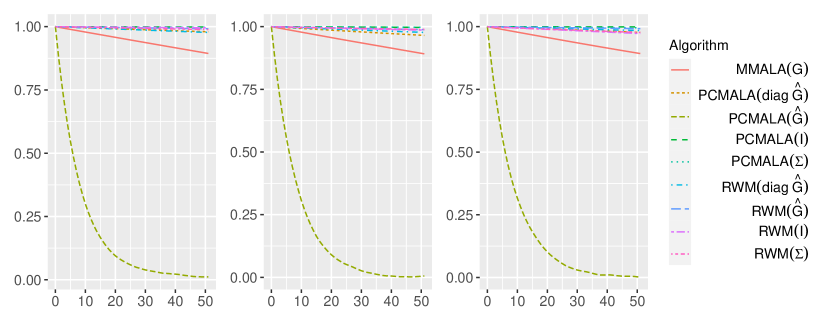
Figure S1: ACF plots for $x^{(1)}$ (left panel), $x^{(175)}$ (center panel), and $x^{(350)}$ (right panel) for the MH chains for the Poisson SGLMM with the log link. In the legend, $G$ refers to $\mathscr{I}^{-1}$ and $\hat{G}$ refers to $\hat{\mathscr{I}}^{-1}$.

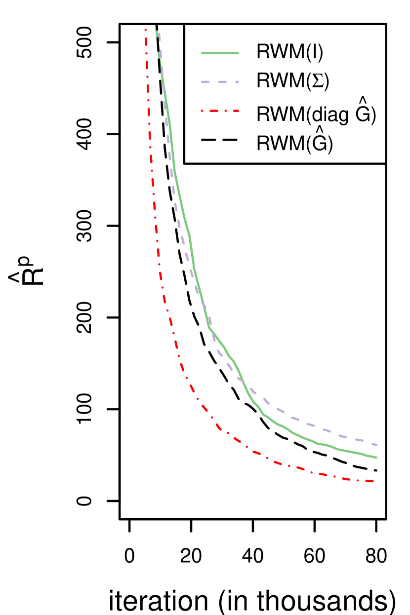
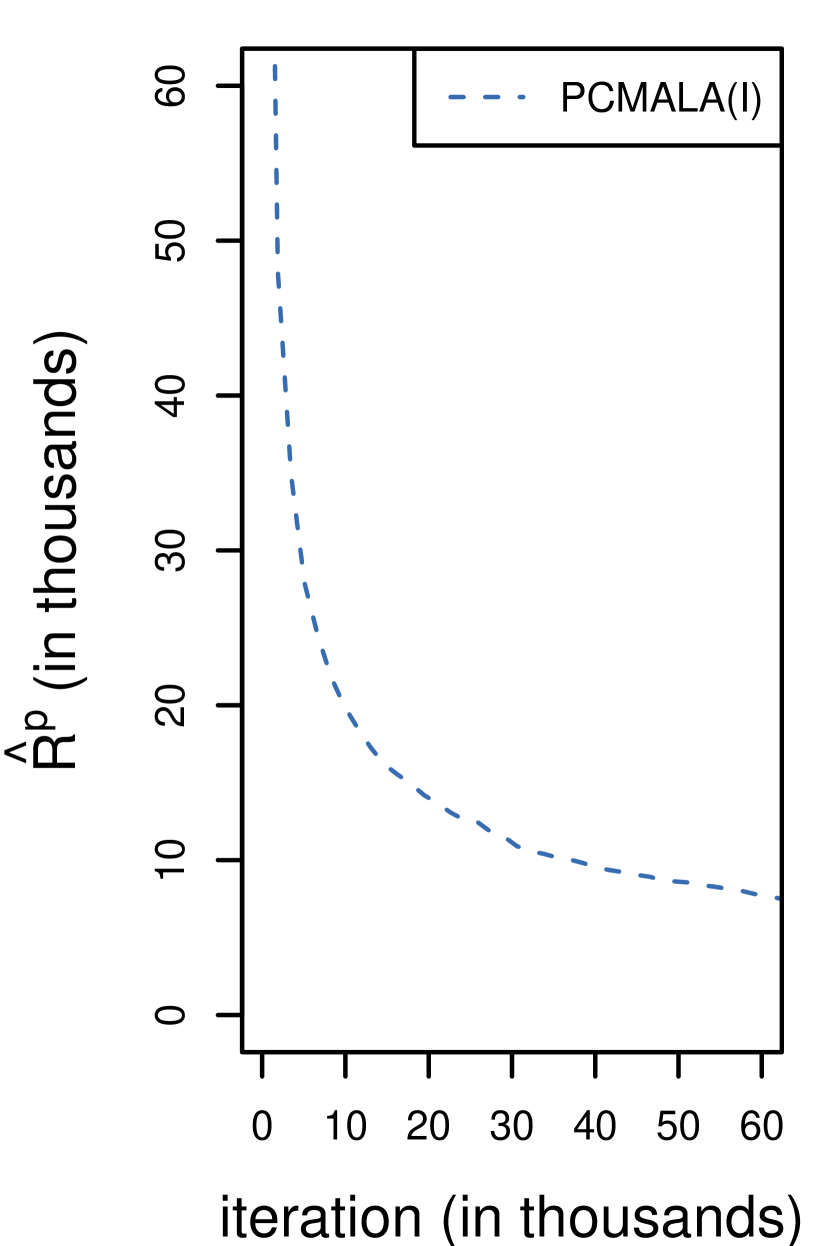
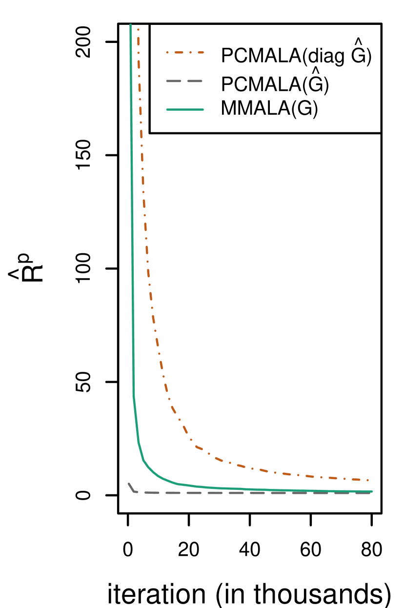
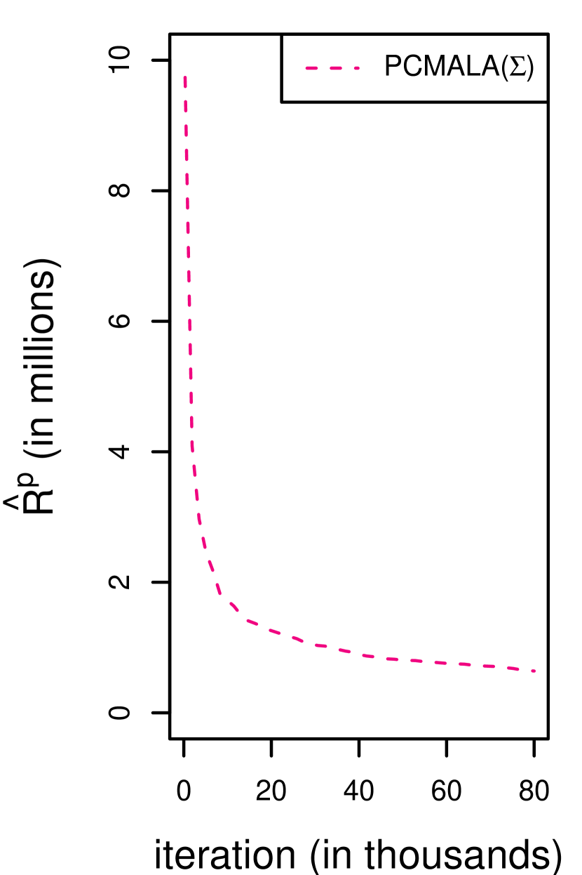
Figure S2: Gelman and Rubin’s $\hat{R}_{p}$ plot from the five parallel MH chains for the Poisson SGLMM with the log link. In the legend, $G$ refers to $\mathscr{I}^{-1}$ and $\hat{G}$ refers to $\hat{\mathscr{I}}^{-1}$.

Table S3: MSJD values for the PCULA chains for the binomial and Poisson SGLMMs

	binomial				Poisson
$G$ matrix	$I$	$\Sigma$	diag $(\hat{\mathscr{I}}^{-1})$	$\hat{\mathscr{I}}^{-1}$	$I$	$\Sigma$	diag $(\hat{\mathscr{I}}^{-1})$	$\hat{\mathscr{I}}^{-1}$
	4.18	0.07	7.42	7.41	0.05	0.05	0.05	126.74

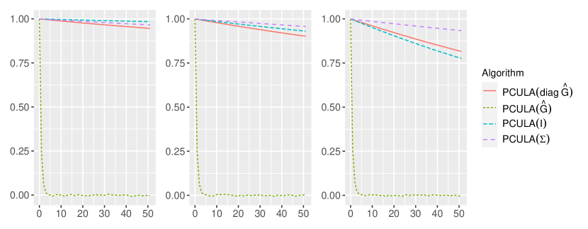
Figure S4: ACF plots for $x^{(1)}$ (left panel), $x^{(175)}$ (center panel), and $x^{(350)}$ (right panel) for the PCULA chains for the Poisson SGLMM with the log link. In the legend, $\hat{G}$ refers to $\hat{\mathscr{I}}^{-1}$.

References

- Besag (1994) Besag, J. (1994), “Comments on ”Representations of knowledge in complex systems” by U. Grenander and M. I. Miller,” J. Roy. Statist. Soc. Ser. B, 56, 591–592.
- Brooks and Gelman (1998) Brooks, S. P. and Gelman, A. (1998), “General methods for monitoring convergence of iterative simulations,” Journal of Computational and Graphical Statistics, 7, 434–455.
- Chen et al. (2020) Chen, Y., Dwivedi, R., Wainwright, M. J., and Yu, B. (2020), “Fast mixing of Metropolized Hamiltonian Monte Carlo: Benefits of multi-step gradients.” J. Mach. Learn. Res., 21, 92–1.
- Chewi et al. (2021) Chewi, S., Lu, C., Ahn, K., Cheng, X., Le Gouic, T., and Rigollet, P. (2021), “Optimal dimension dependence of the Metropolis-adjusted Langevin algorithm,” in Conference on Learning Theory, PMLR, 1260–1300.
- Christensen et al. (2001) Christensen, O. F., Møller, J., and Waagepetersen, R. P. (2001), “Geometric Ergodicity of Metropolis-Hastings Algorithms for Conditional Simulation in Generalized Linear Mixed Models,” Methodology and Computing in Applied Probability, 3, 309–327.
- Christensen et al. (2005) Christensen, O. F., Roberts, G. O., and Rosenthal, J. S. (2005), “Scaling limits for the transient phase of local Metropolis–Hastings algorithms,” Journal of the Royal Statistical Society: Series B (Statistical Methodology), 67, 253–268.
- Christensen et al. (2006) Christensen, O. F., Roberts, G. O., and Sköld, M. (2006), “Robust Markov chain Monte Carlo methods for spatial generalized linear mixed models,” Journal of Computational and Graphical Statistics, 15, 1–17.
- Diggle et al. (1998) Diggle, P. J., Tawn, J. A., and Moyeed, R. A. (1998), “Model-based geostatistics,” Applied Statistics, 47, 299–350.
- Durmus and Moulines (2015) Durmus, A. and Moulines, É. (2015), “Quantitative bounds of convergence for geometrically ergodic Markov chain in the Wasserstein distance with application to the Metropolis Adjusted Langevin Algorithm,” Statistics and Computing, 25, 5–19.
- Durmus and Moulines (2017) Durmus, A. and Moulines, E. (2017), “Nonasymptotic convergence analysis for the unadjusted Langevin algorithm,” The Annals of Applied Probability, 27, 1551–1587.
- Durmus and Moulines (2019) — (2019), “High-dimensional Bayesian inference via the unadjusted Langevin algorithm,” Bernoulli, 25, 2854–2882.
- Dwivedi et al. (2019) Dwivedi, R., Chen, Y., Wainwright, M. J., and Yu, B. (2019), “Log-concave sampling: Metropolis-Hastings algorithms are fast,” Journal of Machine Learning Research, 20, 1–42.
- Ermak (1975) Ermak, D. L. (1975), “A computer simulation of charged particles in solution. I. Technique and equilibrium properties,” The Journal of Chemical Physics, 62, 4189–4196.
- Evangelou and Roy (2019) Evangelou, E. and Roy, V. (2019), “Estimation and prediction for spatial generalized linear mixed models with parametric links via reparameterized importance sampling,” Spatial Statistics, 29, 289–315.
- Geyer (1994) Geyer, C. J. (1994), “On the convergence of Monte Carlo maximum likelihood calculations,” Journal of the Royal Statistical Society, Series B, 56, 261–274.
- Girolami and Calderhead (2011) Girolami, M. and Calderhead, B. (2011), “Riemann Manifold Langevin and Hamiltonian Monte Carlo Methods,” Journal of the Royal Statistical Society: Series B (Statistical Methodology), 73, 123–214.
- Gorham et al. (2019) Gorham, J., Duncan, A. B., Vollmer, S. J., and Mackey, L. (2019), “Measuring sample quality with diffusions,” The Annals of Applied Probability, 29, 2884–2928.
- Grenander and Miller (1994) Grenander, U. and Miller, M. I. (1994), “Representations of knowledge in complex systems,” Journal of the Royal Statistical Society: Series B (Methodological), 56, 549–581.
- Haario et al. (2001) Haario, H., Saksman, E., and Tamminen, J. (2001), “An adaptive Metropolis algorithm,” Bernoulli, 7, 223–242.
- Hastings (1970) Hastings, W. K. (1970), “Monte Carlo Sampling Methods Using Markov Chains and their Applications,” Biometrika, 13, 97–109.
- Jarner and Hansen (2000) Jarner, S. F. and Hansen, E. (2000), “Geometric ergodicity of Metropolis algorithms,” Stochastic Processes and Their Applications, 85, 341–361.
- Jarner and Tweedie (2003) Jarner, S. F. and Tweedie, R. L. (2003), “Necessary conditions for geometric and polynomial ergodicity of random-walk-type Markov chains,” Bernoulli, 9, 559–578.
- Latuszynski et al. (2011) Latuszynski, K., Roberts, G. O., Thiery, A., and Wolny, K. (2011), “Discussion of “Riemann Manifold Langevin and Hamiltonian Monte Carlo Methods” by M. Girolami, and B. Calderhead,” Journal of the Royal Statistical Society: Series B (Statistical Methodology), 73, 188–189.
- Lee et al. (2020) Lee, Y. T., Shen, R., and Tian, K. (2020), “Logsmooth gradient concentration and tighter runtimes for Metropolized Hamiltonian Monte Carlo,” in Conference on learning theory, PMLR, 2565–2597.
- Livingstone (2021) Livingstone, S. (2021), “Geometric Ergodicity of the Random Walk Metropolis with Position-Dependent Proposal Covariance,” Mathematics, 9, 341.
- Livingstone et al. (2019) Livingstone, S., Betancourt, M., Byrne, S., and Girolami, M. (2019), “On the geometric ergodicity of Hamiltonian Monte Carlo,” Bernoulli, 25, 3109–3138.
- Livingstone and Girolami (2014) Livingstone, S. and Girolami, M. (2014), “Information-geometric Markov chain Monte Carlo methods using diffusions,” Entropy, 16, 3074–3102.
- Mangoubi and Smith (2021) Mangoubi, O. and Smith, A. (2021), “Mixing of Hamiltonian Monte Carlo on strongly log-concave distributions: Continuous dynamics,” The Annals of Applied Probability, 31, 2019–2045.
- Mengersen and Tweedie (1996) Mengersen, K. and Tweedie, R. L. (1996), “Rates of convergence of the Hastings and Metropolis algorithms,” The Annals of Statistics, 24, 101–121.
- Metropolis et al. (1953) Metropolis, N., Rosenbluth, A. W., Rosenbluth, M. N., Teller, A. H., and Teller, E. (1953), “Equation of State Calculations by Fast Computing Machines,” The journal of chemical physics, 21, 1087–1092.
- Meyn and Tweedie (1993) Meyn, S. P. and Tweedie, R. L. (1993), Markov Chains and Stochastic Stability, London: Springer Verlag.
- Møller et al. (1998) Møller, J., Syversveen, A. R., and Waagepetersen, R. P. (1998), “Log gaussian cox processes,” Scandinavian journal of statistics, 25, 451–482.
- Neal (2011) Neal, R. M. (2011), Handbook of Markov chain Monte Carlo, Boca Raton, FL: CRC Press, chap. MCMC using Hamiltonian dynamics, 113–162.
- Neal (2012) — (2012), Bayesian learning for neural networks, vol. 118, Springer Science & Business Media.
- Parisi (1981) Parisi, G. (1981), “Correlation Functions and Computer Simulations,” Nuclear Physics B, 180, 378–384.
- Qin and Hobert (2021) Qin, Q. and Hobert, J. P. (2021), “On the limitations of single-step drift and minorization in Markov chain convergence analysis,” The Annals of Applied Probability, 31, 1633–1659.
- Robert and Casella (2004) Robert, C. and Casella, G. (2004), Monte Carlo Statistical Methods, Springer, New York, 2nd ed.
- Roberts and Rosenthal (1998) Roberts, G. O. and Rosenthal, J. S. (1998), “Optimal scaling of discrete approximations to Langevin diffusions,” Journal of the Royal Statistical Society: Series B (Statistical Methodology), 60, 255–268.
- Roberts and Rosenthal (2009) — (2009), “Examples of adaptive MCMC,” Journal of Computational and Graphical Statistics, 18, 349–367.
- Roberts and Stramer (2002) Roberts, G. O. and Stramer, O. (2002), “Langevin Diffusions and Metropolis-Hastings Algorithms,” Methodology and computing in applied probability, 4, 337–357.
- Roberts and Tweedie (1996a) Roberts, G. O. and Tweedie, R. L. (1996a), “Exponential convergence of Langevin distributions and their discrete approximations,” Bernoulli, 2, 341–363.
- Roberts and Tweedie (1996b) — (1996b), “Geometric Convergence and Central Limit theorems for Multidimensional Hastings and Metropolis Algorithms,” Biometrika, 83, 95–110.
- Rosenthal (1995) Rosenthal, J. S. (1995), “Minorization conditions and convergence rates for Markov Chain Monte Carlo,” Journal of the American Statistical Association, 90, 558–566.
- Rossky et al. (1978) Rossky, P. J., Doll, J., and Friedman, H. (1978), “Brownian dynamics as smart Monte Carlo simulation,” The Journal of Chemical Physics, 69, 4628–4633.
- Roy (2020) Roy, V. (2020), “Convergence diagnostics for Markov chain Monte Carlo,” Annual Review of Statistics and Its Application, 7, 387–412.
- Roy et al. (2016) Roy, V., Evangelou, E., and Zhu, Z. (2016), “Efficient estimation and prediction for the Bayesian binary spatial model with flexible link functions,” Biometrics, 72, 289–298.
- Roy and Hobert (2007) Roy, V. and Hobert, J. P. (2007), “Convergence rates and asymptotic standard errors for MCMC algorithms for Bayesian probit regression,” Journal of the Royal Statistical Society, Series B, 69, 607–623.
- Stramer and Roberts (2007) Stramer, O. and Roberts, G. O. (2007), “On Bayesian Analysis of Nonlinear Continuous-time Autoregression Models,” Journal of Time Series Analysis, 28, 744–762.
- Taylor (2015) Taylor, K. B. (2015), “Exact algorithms for simulation of diffusions with discontinuous drift and robust curvature Metropolis-adjusted Langevin algorithms,” Ph.D. thesis, University of Warwick.
- Vats et al. (2019) Vats, D., Flegal, J. M., and Jones, G. L. (2019), “Multivariate output analysis for Markov chain Monte Carlo,” Biometrka, 106, 321–337.
- Vempala and Wibisono (2019) Vempala, S. and Wibisono, A. (2019), “Rapid convergence of the unadjusted Langevin algorithm: Isoperimetry suffices,” Advances in neural information processing systems, 32.
- Wang and Roy (2018) Wang, X. and Roy, V. (2018), “Geometric ergodicity of Pólya-Gamma Gibbs sampler for Bayesian logistic regression with a flat prior,” Electronic Journal of Statistics, 12, 3295–3311.
- Wu et al. (2021) Wu, K., Schmidler, S., and Chen, Y. (2021), “Minimax mixing time of the Metropolis-adjusted Langevin algorithm for log-concave sampling,” arXiv preprint arXiv:2109.13055.
- Xifara et al. (2014) Xifara, T., Sherlock, C., Livingstone, S., Byrne, S., and Girolami, M. (2014), “Langevin diffusions and the Metropolis-adjusted Langevin algorithm,” Statistics & Probability Letters, 91, 14–19.
- Zhang (2002) Zhang, H. (2002), “On estimation and prediction for spatial generalized linear mixed models,” Biometrics, 58, 129–136.