Sausages

Abstract.

The shift locus is the space of normalized polynomials in one complex variable for which every critical point is in the attracting basin of infinity. The method of sausages gives a (canonical) decomposition of the shift locus in each degree into (countably many) codimension 0 submanifolds, each of which is homeomorphic to a complex algebraic variety. In this paper we explain the method of sausages, and some of its consequences.

1. Sausages

For each integer $q\geq 2$ the shift locus $\SS_{q}$ is the set of degree $q$ polynomials $f$ in one complex variable of the form

$$f(z):=z^{q}+a_{2}z^{q-2}+a_{3}z^{q-3}+\cdots+a_{q}$$

for which every critical point of $f$ is in the attracting basin of $\infty$. One can think of $\SS_{q}$ as a open submanifold of $\mathbb{C}^{q-1}$; understanding its topology is a fundamental problem in complex dynamics. For example, when $q=2$ the complement of $\SS_{2}$ in $\mathbb{C}$ is the Mandelbrot set. Knowing that $\SS_{2}$ is homeomorphic to a cylinder implies the famous theorem of Douady–Hubbard that the Mandelbrot set is connected.

Although the $\SS_{q}$ are highly transcendental spaces, the method of sausages (which we explain in this section) shows that each $\SS_{q}$ has a canonical decomposition into codimension 0 submanifolds whose interiors are homeomorphic to certain explicit algebraic varieties. From this one can deduce a considerable amount about the topology of $\SS_{q}$, especially in low degree.

The construction of sausages has several steps, and goes via an intermediate construction that associates, to each polynomial $f$ in $\SS_{q}$, a certain combinatorial object called a dynamical elamination.

1.1. Green’s function

Let $K$ be a compact subset of $\mathbb{C}$ with connected complement $\Omega_{K}:=\mathbb{C}-K$. If $K$ has positive logarithmic capacity (for example, if the Hausdorff dimension is positive) then there is a canonical Green’s function $g:\Omega_{K}\to\mathbb{R}^{+}$ satisfying

1. $g$ is harmonic;

2. $g$ extends continuously to $0$ on $K$; and

3. $g$ is asymptotic to $\log{|z|}$ near infinity (in the sense that $g(z)-\log{|z|}$ is harmonic near infinity).

There is a unique germ near infinity of a holomorphic function $\phi$, tangent to the identity at $\infty$, for which $g=\log|\phi(z)|$.

1.2. Filled Julia Set

Let $f$ be a degree $q$ complex polynomial. After conjugacy by a complex affine transformation $z\to\alpha z+\beta$ we may assume that $f$ is normalized; i.e. of the form

$$f(z):=z^{q}+a_{2}z^{q-2}+a_{3}z^{q-3}+\cdots+a_{q}$$

The filled Julia set $K(f)$ is the set of complex numbers $z$ for which the iterates $f^{n}(z)$ are (uniformly) bounded. It is a fact that $K(f)$ is compact, and its complement $\Omega_{f}:=\mathbb{C}-K(f)$ is connected. The union $\hat{\Omega}_{f}:=\Omega_{f}\cup\infty$ is the attracting basin of $\infty$.

Böttcher’s Theorem (see e.g. [21] Thm. 9.1) says that $f$ is holomorphically conjugate near infinity to the map $z\to z^{q}$. For normalized $f$, the germ of the conjugating map $\phi$ (i.e. $\phi$ so that $\phi(f(z))=\phi(z)^{q}$) is uniquely determined by requiring that $\phi$ is tangent to the identity at infinity. The (real-valued) function $g(z):=\log|\phi(z)|$ is harmonic, and satisfies the functional equation $g(f(z))=q\cdot g(z)$. We may extend $g$ via this functional equation to all of $\Omega_{f}$ and observe that $g$ so defined is the Green’s function of $K(f)$.

1.3. Maximal domain of $\phi^{-1}$

Let $\overline{\mathbb{D}}\subset\mathbb{C}$ denote the closed unit disk, and $\mathbb{E}:=\mathbb{C}-\overline{\mathbb{D}}$ the exterior. We will use logarithmic coordinates $h=\log(|z|)$ and $\theta=\arg(z)$ on $\mathbb{E}$ and on Riemann surfaces obtained from $\mathbb{E}$ by cut and paste. Note that $g=h\phi$ where $g$ and $\phi$ are as in § 1.1.

For any $K$ with Green’s function $g$ and associated $\phi$ we can analytically continue $\phi^{-1}$ from infinity along radial lines of $\mathbb{E}$. The image of these radial lines under $\phi^{-1}$ are the descending gradient flowlines of $g$ (i.e. the integral curves of $-\text{grad}(g)$), and we can analytically continue $\phi^{-1}$ until the gradient flowlines run into critical points of $g$. Figure 1 shows some gradient flowlines of $g$ for a Cantor set $K$.

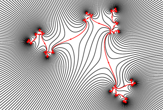
Figure 1. Gradient flowlines of $g$ for a Cantor set $K$

Note that some critical points of $g$ might have multiplicity greater than one; however because $g$ is harmonic, the multiplicity of every critical point is finite, and the critical points of $g$ are isolated and can accumulate (in ${\hat{\mathbb{C}}}$) only on $K$. With this proviso about multiplicity, we want to do a sort of ‘Morse theory’ for the function $g$.

Let $L^{\prime}$ be the union of the segments of the gradient flowlines of $g$ descending from all the critical points of $g$; in Figure 1 these are in red (gray, for black and white reproduction). Then $\Omega_{K}-L^{\prime}$ is the image of the maximal (radial) analytic extension of $\phi^{-1}$. The domain of this maximal extension $\phi^{-1}$ may be described as follows. For $w\in\mathbb{E}$ define the radial segment $\sigma(w)\subset\mathbb{E}$ to be the set of points $z$ with $\arg(z)=\arg(w)$ and $|z|\leq|w|$. The height of $\sigma$, denoted $h(\sigma)$, is $\log(|w|)$. The domain of $\phi^{-1}$ is $\mathbb{E}-L$ where $L$ is the union of a countable proper (in $\mathbb{E}$) collection of radial segments.

If $K=K(f)$ for a polynomial $f$, the critical points of $g$ are the critical points and critical preimages of $f$; i.e. points $z$ for which $(f^{n})^{\prime}(z)=0$ for some positive $n$. Thus $L^{\prime}$ is nearly $f$-invariant: the image $f(L^{\prime})$ is equal to $L^{\prime}\cup\ell^{\prime}$ where $\ell^{\prime}$ is the (finite!) set of descending flowlines from the critical values of $f$ in $\Omega_{f}$ (which are themselves not typically critical).

Likewise the map $z\to z^{q}$ on $\mathbb{E}$ takes $L$ to $L\cup\ell$ where $\ell$ is a finite set of radial segments mapped by $\phi^{-1}$ to $\ell^{\prime}$.

1.4. Cut and Paste

Let $c$ be a critical point of $g$ and let $L^{\prime}_{c}$ be the union of the gradient flowlines of $g$ descending from $c$ (and for simplicity, here and in the sequel let’s suppose these flowlines do not run into another critical point). Then $L^{\prime}_{c}$ is the union of $n+1$ proper embedded rays from $c$ to $K$ where $n$ is the multiplicity of $c$ as a critical point (these rays extend continuously to $K$ when the components of $K$ are locally connected; otherwise they may ‘limit to’ a prime end of a component of $K$). There is a corresponding collection $L_{c}$ of $n+1$ radial segments $\sigma_{j}:=\sigma(w_{j})$ all of the same height, where indices are circularly ordered according to the arguments of the $w_{j}$. The map $\phi^{-1}$ extends continuously along radial lines from infinity all the way to the $w_{j}$: the $w_{j}$ all map to $c$. But any ‘extension’ of $\phi^{-1}$ over $L_{c}$ will be multivalued. We can repair this multivaluedness by cut and paste: cut open $\mathbb{E}$ along the segments $L_{c}$ to create two copies $\sigma_{j}^{+}$ resp. $\sigma_{j}^{-}$ for each $\sigma_{j}$ on the ‘left’ resp. ‘right’ in the circular order. Then glue each segment $\sigma_{j}^{-}$ to $\sigma_{j+1}^{+}$ by a homeomorphism respecting absolute value. Under this operation the collection of segments $L_{c}$ are reassembled into an ‘asterisk’ which resembles the cone on $n+1$ points; see Figure 2.

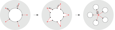
Figure 2. Cut and paste over $L_{c}$ of multiplicity 4

The result is a new Riemann surface for which the map $\phi^{-1}$ now extends (analytically and single-valuedly) over the (cut-open and reglued) image of $L_{c}$, whose image is exactly $L^{\prime}_{c}$.

If we perform this cut and paste operation simultaneously for all the different $L_{c}$ making up $L$, the Riemann surface $\mathbb{E}$ is reassembled into a new Riemann surface $\Omega$ so that $\phi^{-1}$ extends to an isomorphism $\phi^{-1}:\Omega\to\Omega_{K}$.

If $K=K(f)$ for a polynomial $f$, then the map $z\to z^{q}$ on $\mathbb{E}$ descends to a well-defined degree $q$ holomorphic self-map $F:\Omega\to\Omega$ and $\phi^{-1}$ conjugates $F|\Omega$ to $f|\Omega_{f}$.

1.5. Elaminations

It is useful to keep track of the partition of $L^{\prime}$ and $L$ into finite collections $L^{\prime}_{c}$ and $L_{c}$ associated to the critical points $c$ of $g$.

For each critical point $c$ of multiplicity $n$ we span the $n+1$ segments of $L_{c}$ by an ideal hyperbolic $(n+1)$-gon in $\overline{\mathbb{D}}$. The segments of $L_{c}$ become the tips and the ideal polygon becomes the vein of a leaf of multiplicity $n$ in an object called an extended lamination — or elamination for short. When every critical point has multiplicity 1, we say the elamination is simple. See Figures 3 and 7 for examples of simple elaminations. The key topological property of elaminations is that the veins associated to different leaves do not cross. This is equivalent to the fact that the result $\Omega$ of cut and paste along $L$ is a planar surface (because it is isomorphic to $\Omega_{X}\subset\mathbb{C}$).

Elaminations are introduced and studied in [11]. The set ${\mathcal{EL}}$ of elaminations becomes a space with respect to a certain topology (the collision topology), and can be given the structure of a disjoint union of (countable dimensional) complex manifolds. For example, the space of elaminations with $n-1$ leaves (counted with multiplicity) is homeomorphic (but not biholomorphic) to the space of degree $n$ normalized polynomials with no multiple roots.

1.6. Dynamical Elaminations

Figure 3 depicts the elamination associated to $K(f)$ for a degree 3 polynomial $f$. The critical leaves — i.e. the leaves with tips $L_{c}$ associated to $c$ a critical point of $f$ — are in red. Every other leaf corresponds to a precritical point of $f$ (which are critical points of the Green’s function). This elamination is simple: every leaf has exactly two tips.

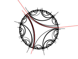
Figure 3. Simple dynamical elamination of degree $3$; critical leaves are in red

Let $\Lambda$ denote the elamination associated to $L$. Note that $\Lambda$ depends not just on $L$ as a set of segments, but also on their partition into subsets $L_{c}$.

The map $z\to z^{q}$ on $\mathbb{E}$ acts on segments and therefore also on leaves, with the following exception. If $\ell$ is a leaf whose tips have arguments that all differ by integer multiples of $2\pi/q$ then these segments will have the same image under $z\to z^{q}$. Since leaves should have at least two tips (by convention), if $\ell$ is a leaf all of whose tips have arguments that differ by integer multiples of $2\pi/q$ then the image of $\ell$ under $z\to z^{q}$ is undefined.

Suppose $K=K(f)$ for a degree $q$ polynomial. Let $C$ denote the critical leaves of $L$ (those associated to critical points of $f$). The map $z\to z^{q}$ takes leaves to leaves in the obvious sense, and takes $\Lambda-C$ to $\Lambda$.

We say an elamination $\Lambda$ is a degree $q$ dynamical elamination if

1. it has finitely many leaves $C$ each of whose arguments differ by integer multiples of $2\pi/q$ (the critical leaves);

2. the map $z\to z^{q}$ takes $\Lambda-C$ to $\Lambda$; and

3. every leaf has exactly $q$ preimages.

A degree $q$ dynamical elamination is maximal if there are $q-1$ critical leaves, counted with multiplicity.

The elamination $\Lambda$ associated to a degree $q$ polynomial $f$ is a degree $q$ dynamical elamination. It is maximal if and only if all the critical points of $f$ are in $\Omega_{f}$.

A set of (non-crossing) leaves $C$, each with arguments that differ by integer multiples of $2\pi/q$ is called a degree $q$ critical set. A critical set is maximal if there are $q-1$ leaves counted with multiplicity. It turns out that every maximal degree $q$ critical set $C$ is exactly the set of critical leaves of a unique (maximal) degree $q$ dynamical elamination $\Lambda$; see [11] Prop. 5.3. The set of maximal degree $q$ dynamical elaminations is denoted $\mathcal{DL}_{q}$. As a subset of ${\mathcal{EL}}$ it has the structure of an open complex manifold of dimension $q-1$ with local coordinates coming from the (endpoints of) segments of $C$ (at least at a generic $\Lambda$).

1.7. The Shift Locus

For each degree $q$ the Shift Locus $\SS_{q}$ is the space of degree $q$ normalized polynomials $f(z):=z^{q}+a_{2}z^{q-2}+a_{3}z^{q-3}+\cdots+a_{q}$ for which every critical point is in the basin of infinity $\Omega_{f}$. The coefficients $a_{2},\cdots,a_{q}$ are coordinates on $\SS_{q}$ realizing it as an open subset of $\mathbb{C}^{q-1}$.

A polynomial $f$ is in $\SS_{q}$ if and only if the Julia set of $f$ is a Cantor set on which $f$ is uniformly expanding (for some metric). Thus for such polynomials, $J(f)=K(f)$ and $\Omega_{f}$ is the entire Fatou set (i.e. the maximal domain of normality of $f$ and its iterates; see e.g. [21]).

Suppose $f\in\SS_{q}$ with associated dynamical elamination $\Lambda$. Since all critical points of $f$ are in $\Omega_{f}$, it follows that $\Lambda$ is maximal; thus there is a map $\SS_{q}\to\mathcal{DL}_{q}$ called the Böttcher map. Conversely, if $\Lambda$ is any maximal degree $q$ dynamical elamination, and $\Omega$ is obtained from $\mathbb{E}$ by cut and paste along $\Lambda$, then $F|\Omega$ extends (topologically) over the space of ends of $\Omega$ to define a degree $q$ self-map $\bar{F}$ of a topological sphere $\bar{\Omega}\cong S^{2}$. It turns out that there is a canonical conformal structure on $\bar{\Omega}$ extending that on $\Omega$ so that $\bar{F}$ is holomorphic. After choosing suitable coordinates on $\bar{\Omega}$ near $\infty$ the map $\bar{F}$ becomes a degree $q$ normalized polynomial, which is contained in $\SS_{q}$. The analytic content of this theorem is essentially due to de Marco–McMullen; see e.g. [16] Thm. 7.1 or [11] Thm. 5.4 for a different proof.

Thus the Böttcher map $\SS_{q}\to\mathcal{DL}_{q}$ is a homeomorphism (and in fact an isomorphism of complex manifolds).

1.8. Stretching and Spinning

There is a (multiplicative) $\mathbb{R}^{+}$ action on ${\mathcal{EL}}$ called stretching where $t\in\mathbb{R}^{+}$ acts on $\Lambda$ by multiplying the $h$ coordinate of every leaf by $t$. This action is free and proper. It preserves $\mathcal{DL}_{q}$ for each $q$, and shows that $\mathcal{DL}_{q}$ (and therefore also $\SS_{q}$) is homeomorphic to the product of $\mathbb{R}$ with a manifold of (real) dimension $2q-3$. It is convenient for what follows to define $\mathcal{DL}_{q}^{\prime}$ to be the open subspace of $\mathcal{DL}_{q}$ for which the highest critical leaf has $\log_{q}(h)\in(-1/2,1/2)$. By suitably ‘compressing’ orbits of the $\mathbb{R}^{+}$ action we see there is a homeomorphism $\mathcal{DL}_{q}\to\mathcal{DL}_{q}^{\prime}$.

There is also an $\mathbb{R}$ action on ${\mathcal{EL}}$ called spinning where $t\in\mathbb{R}$ simultaneously rotates the arguments of leaves of height $h$ by $th$. This makes literal sense for the (finitely many) leaves of greatest height. When leaves of lesser height are collided by those of greater height the shorter leaf is ‘pushed over’ the taller one; the precise details are explained in [11] § 3.2. This $\mathbb{R}$ action also preserves each $\mathcal{DL}_{q}$. The closure of the $\mathbb{R}$-orbits in each $\mathcal{DL}_{q}$ are real tori, and the $\mathbb{R}$-orbits sit in these tori as parallel lines of constant slope. A typical $\mathbb{R}$-orbit has closure which is a torus of real dimension $q-1$, but if some critical leaves have multiplicity $>1$ or if distinct critical leaves have rationally related heights, the closure will be a torus of lower dimension.

Stretching and spinning combine to give an action of the (oriented) affine group $\mathbb{R}\rtimes\mathbb{R}^{+}$ of the line on ${\mathcal{EL}}$ and on each individual $\mathcal{DL}_{q}$.

1.9. Sausages

Suppose $K=K(f)$ for a degree $q$ polynomial. The map $f$ is algebraic, but the domain $\Omega_{f}$ is transcendental. When we move to the elamination side, the map $z\to z^{q}$ and the domain $\mathbb{E}$ are (semi)-algebraic, but the combinatorics of $L$ is hard to understand. Sausages are a way to find a substitute for $(f,\Omega_{f})$ for which both the map and the domain are algebraic and more comprehensible.

The idea of sausages is to find a dynamically invariant way to cut up the domain $\Omega$ into a tree of Riemann spheres, so that $F$ induces polynomial maps between these spheres. The sausage map is not holomorphic, but it induces homeomorphisms between certain codimension 0 submanifolds of $\mathcal{DL}_{q}^{\prime}$ and certain explicit algebraic varieties whose topology is in some ways much easier to understand.

Now let’s discuss the details of the construction. First consider the map $z\to z^{q}$ on $\mathbb{E}$ alone. Let $h:=\log(|z|)$ and $\theta=\arg(z)$ be cylindrical coordinates on $\mathbb{E}$, so that $\mathbb{E}$ becomes the half-open cylinder $S^{1}\times\mathbb{R}^{+}$ in $(\theta,h)$-coordinates, and $z\to z^{q}$ becomes the map which is multiplication by $q$ which we denote $\times q$. For each integer $n$ let $I_{n}$ denote the open interval $(q^{n-1/2},q^{n+1/2})$ and let $A_{n}$ be the annulus in $\mathbb{E}$ where $h\in I_{n}$ and let $A=\cup_{n}A_{n}\subset\mathbb{E}$; the complement of $A$ is the countable set of circles with $\log_{q}(h)\in 1/2+\mathbb{Z}$. Then $\times q$ takes $A_{n}$ to $A_{n+1}$.

This data is holomorphic but not algebraic. So let’s choose (rather arbitrarily) an orientation-preserving diffeomorphism $\nu_{0}:I_{0}\to\mathbb{R}$ and for each $n$ define $\nu_{n}:I_{n}\to\mathbb{R}$ by $\nu_{n}(h)=q^{n}\nu_{0}(q^{-n}h)$ (so that by induction the $\nu_{n}$ satisfy $\nu_{n+1}(qh)=q\nu_{n}(h)$ for all $n$ and $h\in I_{n}$), and define $\mu:A\to S^{1}\times\mathbb{R}$ to be the map that sends $(\theta,h)$ to $(\theta,\nu_{n}(h))$ if $(\theta,h)\in A_{n}$. By construction, $\mu$ commutes with multiplication by $q$:

$$\mu(q\theta,qh)=(q\theta,\nu_{n+1}(qh))=(q\theta,q\nu_{n}(h))=q\mu(\theta,h)$$

In other words, $\mu$ semi-conjugates $\times q$ on $A$ to $\times q$ on $S^{1}\times\mathbb{R}$, which (by exponentiating) becomes the map $z\to z^{q}$ on $\mathbb{C}^{*}$, an algebraic map on an algebraic domain. Actually, it is better to keep a separate copy $\mathbb{C}^{*}_{n}:=\mu(A_{n})$ of $\mathbb{C}^{*}$ for each $n$, so that $\mu$ conjugates $\times q$ on $A$ to the self-map of $\cup_{n}\mathbb{C}^{*}_{n}$ which sends each $\mathbb{C}^{*}_{n}$ to $\mathbb{C}^{*}_{n+1}$ by $z\to z^{q}$.

1.10. Sausages and Dynamics

Now suppose we have a dynamical elamination $\Lambda$ with critical leaves $C$ invariant under $z\to z^{q}$. For each $A_{n}$ the tips of $\Lambda$ intersect $A_{n}$ in a finite collection of vertical segments $L_{n}$ (some of which will pass all the way through $A_{n}$) and we can perform cut-and-paste separately on each $A_{n}$ to produce a (typically disconnected) surface $B_{n}$. Furthermore we can perform cut-and-paste on $\mathbb{C}^{*}_{n}$ along the image $\mu(L_{n})$ which, by construction, is compatible with the Riemann surface structure. The result is to cut and paste $\mathbb{C}^{*}_{n}$ into a finite collection of algebraic Riemann surfaces, each individually isomorphic to $\mathbb{C}$ minus a finite set of points and which can be canonically completed to Riemann spheres in such a way that the map $F$ on $\Omega$ descends to a map $\mathfrak{f}$ from this union of Riemann spheres to itself; see Figure 4.

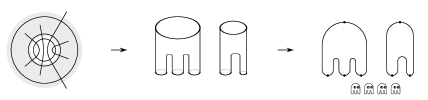
Figure 4. $A_{n}$ is cut and paste into $B_{n}$ which in turn maps to a disjoint union of Riemann spheres

Denote the individual Riemann spheres by $X_{v}$, and by abuse of notation, write $\mathfrak{f}_{v}:X_{v}\to X_{\mathfrak{f}(v)}$ for the restriction of $\mathfrak{f}$ to the component $X_{v}$. By the previous discussion, each map $\mathfrak{f}_{v}$ is holomorphic, so that if we choose suitable coordinates on $X_{v}$ and $X_{\mathfrak{f}(v)}$ the map $\mathfrak{f}_{v}$ becomes a polynomial. There is almost a canonical choice of coordinates, which we explain in the next two sections.

Each $X_{v}$ corresponds to a component $B_{v}$ of some $B_{n}$, and gets a canonical finite set of marked points $Z_{v}^{\prime}$ which correspond to the ‘boundary circles’ of $B_{v}$. The unique boundary circle with greatest $h$ coordinate picks out a point that we can identify with $\infty\in X_{v}$; we denote by $Z_{v}$ the set consisting of the rest of the marked points. The collection of individual Riemann spheres $X_{v}$ can be glued up along their marked points into an infinite genus zero nodal Riemann surface so that the indices $v$ are parameterized by the vertices $v$ of the tree of gluings $T$. This tree is oriented, so that an edge $v$ goes to $w$ if $X_{v}$ is glued along $\infty$ to one of the (non-infinite) marked points of $X_{w}$. We call $w$ the parent of $v$ and $v$ one of the children of $w$. If we make the assumption that no boundary component of any $B_{v}$ contains a critical point (this is the generic case) then each $\zeta\in Z_{w}\subset X_{w}$ is attached to a unique $X_{v}$ for $v$ some child of $w$. If $v$ is a child of $w$, and $X_{v}$ is glued to $X_{w}$ at the point $\zeta\in Z_{w}$, then if $\zeta$ is a critical point of $\mathfrak{f}_{w}$ of multiplicity $m$, the degree of $\mathfrak{f}_{v}$ is $m+1$. By abuse of notation, we denote the induced (simplicial, orientation-preserving) map on $T$ also by $\mathfrak{f}$.

If $\Lambda$ is empty, then $T$ is just a line, and each vertex has a unique child. If $\Lambda$ is nonempty, then since there are only finitely many leaves of greatest height, there is a unique highest vertex $v$ of $T$ with more than one child. Let $w$ be the parent of $v$. The uppermost boundary components of $B_{v}$ and $B_{w}$ are canonically identified with the unit circle $S^{1}:=\mathbb{R}/2\pi\mathbb{Z}$. By identifying these circles with the unit tangent circles at $\infty$ in $X_{v}$ and $X_{w}$ we can choose coordinates on these Riemann spheres so that the tangent to the positive real axis corresponds to the angle $0\in S^{1}$. In these coordinates $X_{v}$ and $X_{w}$ are identified with copies ${\hat{\mathbb{C}}}_{v}$ and ${\hat{\mathbb{C}}}_{w}$ of the Riemann sphere ${\hat{\mathbb{C}}}$, and after precomposing with a suitable complex affine translation, $\mathfrak{f}_{v}$ becomes a normalized degree $q$ polynomial map $\mathfrak{f}_{v}:z\to z^{q}+b_{2}z^{q-2}+\cdots b_{q}$, and the (non-infinite) marked points of $X_{v}$ become the roots of $\mathfrak{f}_{v}$ in ${\hat{\mathbb{C}}}_{v}$.

Vertices of $T$ above $v$ and the maps between their respective Riemann surfaces do not carry any information. Let $w_{1}:=w$ denote the parent of $v$, and inductively let $w_{n}$ be the parent of $w_{n-1}$. Then each $X_{w_{n}}$ has exactly two marked points, which we can canonically identify with $\infty$ and $0$, and the map $\mathfrak{f}_{w_{n-1}}:{\hat{\mathbb{C}}}_{w_{n-1}}\to{\hat{\mathbb{C}}}_{w_{n}}$ is canonically normalized as $z\to z^{q}$.

Since these vertices carry no information, we discard them. Thus we make the convention that $T$ is the rooted tree consisting of $v$ together with its (iterated) children, and we let $\mathfrak{X}$ denote the nodal Riemann surface corresponding to the union of $X_{w}$ with $w$ in $T$. We record the data of the polynomial $\mathfrak{f}_{v}$ associated to the root $v$, though we do not interpret this any more as a map between Riemann spheres, so that $\mathfrak{f}$ is now a map from $\mathfrak{X}-X_{v}$ to $\mathfrak{X}$ and $\mathfrak{f}_{v}$ is a polynomial function on $X_{v}\cong{\hat{\mathbb{C}}}$.

1.11. Tags and sausage polynomials

The choice of a distinguished point on a boundary $S^{1}$ component of some $B_{u}$ is called a tag. Tags are the data we need to choose coordinates on $\mathfrak{X}$ so that every $\mathfrak{f}_{u}$ becomes a polynomial. We may identify this boundary circle with the unit tangent circle at a marked point on $X_{u}$, and think of the tag as data on $X_{u}$. By induction, we can choose tags on $X_{u}$ in the preimage of the tags of $X_{\mathfrak{f}(u)}$ under the map $\mathfrak{f}_{u}:X_{u}\to X_{\mathfrak{f}(u)}$ and inductively define coordinates ${\hat{\mathbb{C}}}_{u}$ on $X_{u}$ for which $\mathfrak{f}_{u}$ is represented by a normalized polynomial map (in general of degree $\leq q$).

Suppose $u$ has parent $u^{\prime}$, and $\infty$ in ${\hat{\mathbb{C}}}_{u}$ is attached at some point $\zeta\in Z_{u^{\prime}}\in{\hat{\mathbb{C}}}_{u^{\prime}}$. Suppose $\zeta$ is a critical point of $\mathfrak{f}_{u^{\prime}}$ with multiplicity $m$. Then $\mathfrak{f}_{u}$ has degree $m+1$. There are $m+1$ different choices of tag at $\zeta$ that map to the tag at $\mathfrak{f}_{u^{\prime}}(\zeta)$, and the different choices affect the normalization of $\mathfrak{f}_{u}$ by precomposing with multiplication by an $(m+1)$st root of unity.

The endpoint of this discussion is that we can recover $\mathfrak{X},\mathfrak{f}$ from the data of a rooted tree $T$, and a set of equivalence classes of pair $(\text{tag},\text{normalized polynomial }\mathfrak{f}_{u})$. Call this data a (degree $q$) sausage polynomial.

A dynamical elamination $\Lambda$ is generic if the critical points of $F$ are all contained in $A$; i.e. if no critical (or by induction, precritical) point has $h$ coordinate with $\log(h)\in 1/2+\mathbb{Z}$. The sausage map is the map that associates a sausage polynomial to a degree $q$ dynamical elamination. A sausage polynomial is generic resp. maximal if it is in the image of a generic resp. maximal dynamical elamination.

A polynomial $\mathfrak{f}_{w}$ associated to a (generic) sausage polynomial has two kinds of critical points. The genuine critical points are those in ${\hat{\mathbb{C}}}_{w}-Z_{w}^{\prime}$ (recall that $Z_{w}^{\prime}$ is $Z_{w}\cup\infty$). The fake critical points are those in $Z_{w}^{\prime}$ ($=\infty\cup Z_{w}$) which correspond to circle components of $B_{w}$ mapping with degree $>1$. For a generic dynamical elamination, the genuine critical points of the associated sausage polynomial are exactly the images of the critical points of the elamination (i.e. the endpoints of the critical leaves) under the sausage map. Thus for a generic maximal sausage polynomial of degree $q$, there are exactly $q-1$ genuine critical points, counted with multiplicity.

For a generic, maximal sausage polynomial, all but finitely many $\mathfrak{f}_{v}$ have degree one. A degree one map uniquely pulls back tags, and has only one possible normalized polynomial representative, namely the identity map $z\to z$. Thus a generic, maximal sausage polynomial is described by a finite amount of combinatorial data together with a finite collection of normalized polynomials. The reader who wants to see some examples should look ahead to § 2.1 and § 2.3.

Let $\mathcal{X}_{q}$ denote the space of generic maximal degree $q$ sausage polynomials. Then $\mathcal{X}_{q}$ is the disjoint union of countably infinitely many components, indexed by the combinatorics of $T$ and the degrees of the normalized polynomials between the associated Riemann spheres. Each component of $\mathcal{X}_{q}$ is a quasiprojective complex variety of complex dimension $q-1$. In fact, each component is an iterated fiber bundle whose base and fibers are certain affine (complex) varieties called Hurwitz varieties, which we shall describe in more detail in § 2.6.

1.12. Sausage space

Recall that $\mathcal{DL}_{q}^{\prime}\subset\mathcal{DL}_{q}$ denotes the set of maximal degree $q$ dynamical elaminations for which the highest critical point has $\log_{q}(h)\in(-1/2,1/2)$. Let $\mathcal{DL}_{q}^{\prime\prime}\subset\mathcal{DL}_{q}^{\prime}$ denote the subspace of generic maximal degree $q$ dynamical elaminations. Then the construction of the previous few sections defines a map $\mathcal{DL}_{q}^{\prime\prime}\to\mathcal{X}_{q}$.

In fact, this map is invertible. Given a sausage polynomial $\mathfrak{X},\mathfrak{f}$ over a tree $T$ with root $v$ we can inductively construct (singular) vertical resp. horizontal foliations on each ${\hat{\mathbb{C}}}_{w}$ as follows. On ${\hat{\mathbb{C}}}_{v}$ we pull back the foliations of $\mathbb{C}^{*}$ by lines resp. circles of constant argument resp. absolute value under the polynomial $\mathfrak{f}_{v}$. Then on every other $w$ we inductively pull back these foliations under $\mathfrak{f}_{w}:{\hat{\mathbb{C}}}_{w}\to{\hat{\mathbb{C}}}_{\mathfrak{f}(w)}$. These foliations all carry coordinates pulled back from $\mathbb{C}^{*}$, and ${\hat{\mathbb{C}}}_{w}$ minus infinity and its marked points becomes isomorphic to a branched Euclidean Riemann surface with ends isomorphic to the ends of (infinite) Euclidean cylinders. We can reparameterize the vertical coordinates on each of these Riemann surfaces by the inverses of the maps $\nu_{n}$, and then glue together the result by matching up boundary circles using tags. This defines an inverse to the map $\mathcal{DL}_{q}^{\prime\prime}\to\mathcal{X}_{q}$ and shows that this map is a homeomorphism. See [11] Thm. 9.20 for details.

1.13. Decomposition of the Shift Locus

Putting together the various constructions we have discussed so far we obtain the following summary:

1. § 1.7: The map that associates to $f\in\SS_{q}$ a maximal degree $q$ dynamical elamination $\Lambda$ gives an isomorphism of complex manifolds $\SS_{q}\to\mathcal{DL}_{q}$.

2. § 1.8: By compressing orbits of the free $\mathbb{R}^{+}$ action on $\mathcal{DL}_{q}$ we obtain a homeomorphism $\mathcal{DL}_{q}\to\mathcal{DL}_{q}^{\prime}$ to the subspace whose largest critical leaf has log height $\log_{q}(h)\in(-1/2,1/2)$.

3. § 1.12: The open dense subset $\mathcal{DL}_{q}^{\prime\prime}\subset\mathcal{DL}_{q}^{\prime}$ of generic dynamical elaminations maps homeomorphically by the sausage map $\mathcal{DL}_{q}^{\prime\prime}\to\mathcal{X}_{q}$.

4. § 1.11: The space $\mathcal{X}_{q}$ is the disjoint union of countably many quasiprojective complex varieties, each of which has the structure of an iterated bundle of affine (Hurwitz) varieties.

In words: the shift locus $\SS_{q}$ in degree $q$ has a canonical decomposition into codimension 0 submanifolds whose interiors are homeomorphic to certain explicit algebraic varieties. It is a fact that we do not explain here (see [11] § 8 especially Thm. 8.11) that the abstract cell complex which combinatorially parameterizes the decomposition of $\SS_{q}$ into these pieces is contractible, so that all the interesting topology of $\SS_{q}$ is localized in the components of $\mathcal{X}_{q}$.

In the remainder of the paper we give examples, and explore some of the consequences of this structure.

2. Sausage Moduli

Each component $Y$ of $\mathcal{X}_{q}$ parameterizes sausages of a fixed combinatorial type. The combinatorial type determines finitely many vertices $u$ for which the (normalized) polynomial $\mathfrak{f}_{u}$ has degree $>1$. The combinatorics constrains these polynomials by imposing conditions on their critical values, for instance that the critical values are required to lie outside a certain (finite) set. Thus, each component has the structure of an algebraic variety which is an iterated fiber bundle, and so that the base and each fiber is something called a Hurwitz Variety.

For this and other reasons, the spaces $\SS_{q}$ and the components $Y$ of which they are built bear a close family resemblance to the kinds of discriminant complements that arise in the study of classical braid groups. The full extent of this resemblance is an open question, partially summarized in Table 2.

2.1. Degree 2

Let $\mathfrak{X},\mathfrak{f}$ be a generic maximal sausage polynomial of degree $2$. The root polynomial $\mathfrak{f}_{v}$ is quadratic and normalized. It has one critical point, necessarily genuine. Thus $\mathfrak{f}_{v}(z):=z^{2}+c$ for some $c\neq 0$. Every other vertex $w$ has a polynomial $\mathfrak{f}_{w}$ of degree one; since polynomials are normalized, $\mathfrak{f}_{w}(z):=z$. Thus all the information is contained in the choice of the (nonzero) constant coefficient $c$ of $\mathfrak{f}_{v}$, so that $\mathcal{X}_{2}=\mathbb{C}^{*}$. The tree $T$ is an infinite dyadic rooted tree, where every vertex is attached to its parent at the points $\pm\sqrt{-c}$; see Figure 5.

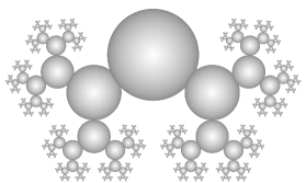
Figure 5. A degree 2 sausage; each vertex is attached to its parent at the points $\pm\sqrt{-c}$.

Furthermore, in this case $\mathcal{DL}_{2}^{\prime}=\mathcal{DL}_{2}^{\prime\prime}$ so that $\SS_{2}$ is homeomorphic (but not holomorphically isomorphic) to $\mathbb{C}^{*}$. As a corollary one deduces the famous theorem of Douady–Hubbard [17] that the Mandelbrot set $\mathcal{M}$ (i.e. $\mathbb{C}-\SS_{2}$) is connected.

2.2. Discriminant Locus

In any degree $q$ there is a unique component of $\mathcal{X}_{q}$ for which all the (genuine) critical points are in the root vertex. Thus $\mathfrak{f}_{v}$ is a degree $q$ normalized polynomial with no fake critical points. Since the marked points $Z_{v}$ of the root vertex are exactly the roots of $\mathfrak{f}_{v}$, this means that $\mathfrak{f}_{v}$ is a normalized polynomial with no critical roots. Equivalently, $\mathfrak{f}_{v}$ has $q$ distinct roots, so that $\mathfrak{f}_{v}$ is in $Y_{q}:=\mathbb{C}^{q-1}-\Delta_{q}$ where $\Delta_{q}$ is the discriminant locus. As is well-known, $Y_{q}$ is a $K(B_{q},1)$ where $B_{q}$ denotes the braid group on $q$ strands.

2.3. Degree 3

Let $\mathfrak{X},\mathfrak{f}$ be a generic maximal sausage polynomial of degree $3$. If the root polynomial $\mathfrak{f}_{v}$ has two genuine critical points we are in the case discussed in § 2.2 and the corresponding component of $\mathcal{X}_{3}$ is a $K(B_{3},1)$. Otherwise, since the root polynomial must have at least one genuine critical point, if it does not have two it must have exactly one and $\mathfrak{f}_{v}$ is of the form $z\to(z-c)^{2}(z+2c)$ for some $c\in\mathbb{C}^{*}$.

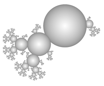
Figure 6. A degree 3 sausage; the root $v$ has $Z_{v}:=\{c,-2c\}$. The child $w_{1}$ has $Z_{w_{1}}:=\{\pm\sqrt{c-d},\pm\sqrt{-2c-d}\}$

The (finite) marked points $Z_{v}$ of ${\hat{\mathbb{C}}}_{v}$ are $c$ and $-2c$, and the root vertex correspondingly has two children $w_{1},w_{2}$ where ${\hat{\mathbb{C}}}_{w_{1}}$ is attached at $c$ and ${\hat{\mathbb{C}}}_{w_{2}}$ is attached at $-2c$. Because $c$ is a double root, the polynomial $\mathfrak{f}_{w_{1}}$ has degree $2$; because $-2c$ is a simple root, the polynomial $\mathfrak{f}_{w_{2}}$ has degree $1$.

Write $\mathfrak{f}_{w_{1}}:z\to z^{2}+d$. If $d\neq c,-2c$ then $Z_{w_{1}}$ has four (non-critical) points (the distinct square roots of $c-d$ and $-2c-d$) and every other $\mathfrak{f}_{u}$ is degree 1. See Figure 6. Thus $c$ and $d$ are moduli parameterizing a single component of $\mathcal{X}_{3}$, and topologically this component is a bundle over $\mathbb{C}^{*}$ whose fiber is homeomorphic to $\mathbb{C}-\{c,-2c\}$.

If $d=c$ or $d=-2c$ then $0$ is a fake critical point for $\mathfrak{f}_{w_{1}}$, and if $u$ is the child of $w_{1}$ for which ${\hat{\mathbb{C}}}_{u}$ is attached at $0$ then $\mathfrak{f}_{u}$ has degree $2$. Since $\mathfrak{f}$ is maximal, there is always some vertex $u^{\prime}$ at finite combinatorial distance from the root for which $\mathfrak{f}_{u^{\prime}}$ has degree $2$ and for which the critical point $0$ of $\mathfrak{f}_{u^{\prime}}$ is genuine. Thus each component of $\mathcal{X}_{3}$ is a bundle over $\mathbb{C}^{*}$ with fiber homeomorphic to $\mathbb{C}$ minus finitely many points.

2.4. The Tautological Elamination

The combinatorics of the components of $\mathcal{X}_{3}$ is quite complicated. Each component of $\mathcal{X}_{3}$ (other than the discriminant complement c.f. § 2.2) is a punctured plane bundle over the curve $\mathbb{C}^{*}$ with parameter $c$, and these components glue together in $\SS_{3}$ to form a bundle over $\mathbb{C}^{*}$ whose fiber $\Omega_{T}$ is homeomorphic to a plane minus a Cantor set.

Actually, there is another description of $\Omega_{T}$ in terms of elaminations. For each degree 3 critical leaf $C$ there is a certain elamination $\Lambda_{T}(C)$ called the tautological elamination which can be defined as follows. Let’s suppose that we have a maximal degree $3$ dynamical elamination with two critical leaves $C$ and $C^{\prime}$, and that $C$ has the greater height. If we fix $C$, then $\Omega_{T}$ parameterizes the space of configurations of $C^{\prime}$.

The elamination $\Lambda_{T}(C)$ is defined as follows. With $C$ fixed, each choice of (noncrossing) $C^{\prime}$ determines a dynamical elamination $\Lambda$. By hypothesis $h(C^{\prime})<h(C)$ and there are only finitely many (perhaps zero) precritical leaves $P$ of $C$ with $h(P)>h(C^{\prime})$. As we vary $C^{\prime}$ the laminations $\Lambda$ also vary (in rather a complicated way) but while $h(P)>h(C^{\prime})$ the leaves $P$ stay fixed under continuous variations of $C^{\prime}$. It might happen that as we vary the leaf $C^{\prime}$ it collides with a leaf $P$ with $h(P)>h(C^{\prime})$; the elamination $\Lambda_{T}(C)$ consists of the cubes $P^{3}$ of all such $P$ (there is a similar, though more complicated construction in higher degrees). The fact that $\Lambda_{T}(C)$ is an elamination is not obvious from this definition.

The result of cut and paste (as in § 1.4) on the annulus $1<|z|<|C|$ (thought of as a subset of $\mathbb{E}$) along $\Lambda_{T}(C)$ is a Riemann surface $\Omega_{T}(C)$ holomorphically isomorphic to the moduli space of degree 3 maximal dynamical elaminations for which $C$ is the unique critical leaf of greatest height. Figure 7 depicts the elamination $\Lambda_{T}(C)$ for a particular value of $C$ whose tips have angles $\pm\pi/3$.

Figure 7. The tautological elamination $\Lambda_{T}(C)$ for $\arg(C)=\pm\pi/6$

These $\Omega_{T}(C)$ are the leaves of a (singular) one complex dimensional holomorphic foliation of $\SS_{3}$.

Although it is not a dynamical elamination, the tautological elamination $\Lambda_{T}(C)$ is in a natural way the increasing union of finite elaminations $\Lambda_{n}$, namely the leaves of the form $P^{3}$ as above where $P$ is a depth $n$ preimage of $C$. Let $\overline{\mathbb{E}}$ denote the closure of $\mathbb{E}$ in $\mathbb{C}$ so that $\overline{\mathbb{E}}=\mathbb{E}\cup S^{1}$, the union of $\mathbb{E}$ with the unit circle. The result $\Omega_{n}$ of cut and pasting $\mathbb{E}$ along $\Lambda_{n}$ is partially compactified by a finite set of circles, obtained from $S^{1}$. By abuse of notation we denote this finite set of circles by $S^{1}\mod\Lambda_{n}$. It turns out that the the components of $\mathcal{X}_{3}\cap\Omega_{T}$ corresponding to sausage polynomials with fixed $c\in\mathbb{C}^{*}$ and for which the second genuine critical point is in a vertex at depth $n+1$ are in bijection with the set of components of $S^{1}\mod\Lambda_{n}$. In fact, more is true.

For each combinatorial type $\mathfrak{X},\mathfrak{f}$ let $u$ be the vertex containing the second genuine critical point (the first, by hypothesis, is contained in the root). We define the depth $n$ of $\mathfrak{X},\mathfrak{f}$ to be the combinatorial distance of $u$ to the root. There is another invariant of $\mathfrak{X},\mathfrak{f}$: the $\ell$-value, defined as follows. Under iteration of $\mathfrak{f}$ (acting on the tree) the vertex $u$ has a length $n$ orbit terminating in the root (note that $\mathfrak{f}(u)$ is not typically equal to the parent of $u$, but it does have the same depth as the parent). The point $\infty$ in ${\hat{\mathbb{C}}}_{u}$ is mapped to $\infty$ in ${\hat{\mathbb{C}}}_{\mathfrak{f}(u)}$ and so on. The product of the degrees of the polynomials $\mathfrak{f}_{\mathfrak{f}^{i}(u)}$ up to but not including the root is some power of $2$; by definition, $\ell$ is this number divided by $2$. The invariants $n$ and $\ell$, taking discrete values, are really invariants of the components of $\mathcal{X}_{3}$ and ipso facto of the components of $\mathcal{X}_{3}\cap\Omega_{T}$.

Here is the relation to $\Lambda_{T}(C)$. Components of $\mathcal{X}_{3}\cap\Omega_{T}$ of depth $n+1$ are in bijective correspondence with components of $S^{1}\mod\Lambda_{n}$, and a component of $\mathcal{X}_{3}\cap\Omega_{T}$ with $\ell$-value $\ell$ corresponds to a component of $S^{1}\mod\Lambda_{n}$ of length $2\pi\ell\cdot 3^{-n}$.

2.5. Combinatorics

Let $N_{3}(n,m)$ denote the number of components of $S^{1}$ mod $\Lambda_{n}$ with depth $n+1$ and $\ell=2^{m}$. We do not know a simple closed form for $N_{3}(n,m)$ and perhaps none exists — one subtle issue is that there are several combinatorially different ways that a component can have a particular $\ell$-value. However, an $\ell$-value of $1$ is special, since it corresponds to an $\mathfrak{f}$ for which $\mathfrak{f}_{\mathfrak{f}^{i}(u)}$ has degree $1$ for all positive $i$. Correspondingly, there is an explicit formula for $N_{3}(n,0)$ that we now give; see [10] Thm. 3.6 for a proof.

First of all, $N_{3}(n,0)$ satisfies the recursion $N_{3}(0,0)=1$, $N_{3}(1,0)=1$ and

$$N_{3}(2n,0)=3N_{3}(2n-1,0)\text{ and }N_{3}(2n+1,0)=3N_{3}(2n,0)-2N_{3}(n,0)$$

Knowing this, one can write down an explicit generating function for $N_{3}(n,0)$; the generating function is $(\beta(t)-1)/3t$ where

$$\beta(t)=\Bigl{(}\sum_{n=0}^{\infty}h(n)t^{n}\Bigr{)}\prod_{j=0}^{\infty}\frac{1}{(1-3t^{2^{j}})}$$

and where the numbers $h(n)$ are defined by

$$h(0)=1\text{ and }h(n)=(-3)^{s(n)}(1-(-2)^{k(n)})$$

where $2^{k(n)}$ is the biggest power of 2 dividing $n$, and $s(n)$ is the sum of the binary digits of $n$.

Table 1 gives values of $N_{3}(n,m)$ for $0\leq n,m\leq 12$. Note that $N_{3}(n,m)=0$ for $n/2<m<n$; see [10] Thm 5.9.

$n\backslash\ell$	1	2	$2^{2}$	$2^{3}$	$2^{4}$	$2^{5}$	$2^{6}$	$2^{7}$	$2^{8}$	$2^{9}$	$2^{10}$	$2^{11}$	$2^{12}$
0	1
1	1	1
2	3	1	1
3	7	6	0	1
4	21	16	3	0	1
5	57	51	13	0	0	1
6	171	149	39	5	0	0	1
7	499	454	117	23	0	0	0	1
8	1497	1348	360	66	9	0	0	0	1
9	4449	4083	1061	207	41	0	0	0	0	1
10	13347	12191	3252	591	126	17	0	0	0	0	1
11	39927	36658	9738	1799	370	81	0	0	0	0	0	1
12	119781	109898	29292	5351	1125	240	33	0	0	0	0	0	1

Table 1. Number of components of length $\ell/3^{n}$ at depth $n$

2.6. Hurwitz Varieties

Let $X$ be a component of $\mathcal{X}_{q}$ parameterizing sausage polynomials of a fixed combinatorial type. $X$ is an iterated bundle whose base and fibers $Y$ are all of the following sort. There are specific vertices $u,w$ with $\mathfrak{f}(u)=w$. The set $Z_{w}\subset{\hat{\mathbb{C}}}_{w}$ is fixed, as is the degree $p$ of $\mathfrak{f}_{u}:{\hat{\mathbb{C}}}_{u}\to{\hat{\mathbb{C}}}_{w}$. Furthermore, for each $\zeta\in Z_{w}$ the ramification data of $\mathfrak{f}_{u}$ at $\zeta$ is specified; i.e. the monodromy of $\mathfrak{f}_{u}^{-1}$ in a small loop around each $\zeta$, thought of as a conjugacy class in the symmetric group on $p$ letters. Then $Y$ is the space of normalized degree $p$ polynomials with the specified ramification data. We call $Y$ a Hurwitz Variety, and observe that each $X$ is an iterated bundle with total (complex) dimension $q-1$ whose base and fibers are all Hurwitz varieties.

The generic case is that the monodromy of $\mathfrak{f}_{u}^{-1}$ in a small loop around each $\zeta\in Z_{w}$ is trivial; i.e. that each $\zeta$ is a regular value. In that case $Y$ is a Zariski open subset of $\mathbb{C}^{p-1}$. In fact, we can say something more precise. Let $\Delta_{p}\subset\mathbb{C}^{p-1}$ be the discriminant variety, i.e. the set of normalized degree $p$ polynomials with a multiple root. For each $\zeta\in Z_{w}$ let $\Delta_{p,\zeta}:=\Delta_{p}+\zeta$ be the translate of $\Delta_{p}$ which parameterizes the set of normalized degree $p$ polynomials $f$ for which $\zeta$ is a critical value. Then

$$Y=\mathbb{C}^{p-1}-\bigcup_{\zeta\in Z_{w}}\Delta_{p,\zeta}$$

It turns out that the topology of $Y$ depends only on the cardinality of $Z_{w}$; see [11] Prop. 9.14. This is not obvious, since the $\Delta_{p,\zeta}$ are singular, and they do not intersect in general position.

2.7. $K(\pi,1)$s

For a finite set $Z\subset\mathbb{C}$ and degree $p$ let $Y_{p}(Z)$ denote the Hurwitz variety of normalized degree $p$ polynomials for which no element of $Z$ is a critical value.

As we remarked already in § 2.2, when $|Z|=1$ the space $Y_{p}(Z)$ is a $K(B_{p},1)$ where $B_{p}$ denotes the braid group on $p$ strands. Furthermore, when $p=2$ the space $Y_{2}(Z)$ may be identified with $\mathbb{C}-Z$ in the obvious way, so that $Y_{2}(Z)$ is a $K(F_{n},1)$ where $F_{n}$ is the free group on $n$ elements, and $n=|Z|$.

It turns out ([11] Thm. 9.17) that $Y_{3}(Z)$ is a $K(\pi,1)$ for any finite set $Z$. This is proved by exhibiting an explicit $\text{CAT}(0)$ 2-complex with the homotopy type of each $Y_{3}(Z)$. One component of $\mathcal{X}_{4}$ is a $K(B_{4},1)$ and all the others are nontrivial iterated fibrations where the fibers are $Y_{2}(Z)$ or $Y_{3}(Z)$s. It follows that every component of $\mathcal{X}_{4}$ is a $K(\pi,1)$, and in fact so is the shift locus $\SS_{4}$ itself (the same is true for simpler reasons of $\SS_{3}$ and $\SS_{2}$).

One knows few example of algebraic varieties which are $K(\pi,1)$s, and fewer methods to construct or certify them (one of the few general methods, which applies to certain complements of hyperplane arrangements, is due to Deligne [15]). Is $Y_{p}(Z)$ a $K(\pi,1)$ for all $p$ and all $Z$?

2.8. Monodromy

For each $p$ and $|Z|$ there is a natural representation (well-defined up to conjugacy) $\pi_{1}(Y_{p}(Z))\to B_{p|Z|}$ defined by the braiding of the $p|Z|$ points $f^{-1}(Z)$ in $\mathbb{C}$ as $f$ varies in $Y_{p}(Z)$. This map is evidently injective when $p=2$ or when $|Z|=1$. Is it injective in any other case? I do not know the answer even when $p=3$ and $|Z|=2$.

Here is one reason to be interested. There is a monodromy representation of $\pi_{1}(\SS_{q})$ into the ‘Cantor braid group’ — i.e. the mapping class group of a disk minus a Cantor set — defined by the braiding of the (Cantor) Julia set $J_{f}$ in $\mathbb{C}$ as $f$ varies in $\SS_{q}$. A priori this representation lands in the mapping class group of the plane minus a Cantor set, but it lifts canonically to the Cantor braid group (which is a central extension) because every $f\in\SS_{q}$ acts in a standard way at infinity. If one forgets the braiding and only considers the permutation action on the Cantor set itself, the image in $\text{Aut}(\text{Cantor Set})$ is known to be precisely equal to the automorphism group of the full (one-sided) shift on a $q$ element alphabet, by a celebrated theorem of Blanchard–Devaney–Keen [5]. However, this action of $\pi_{1}(\SS_{q})$ on the Cantor set alone is very far from faithful.

The automorphism group of the Cantor set is to the Cantor braid group as a finite symmetric group is to a (finite) braid group. It is natural to ask: is the monodromy representation from $\pi_{1}(\SS_{q})$ to the Cantor braid group injective? It turns out that the restriction of the monodromy representation to the image of $\pi_{1}(Y_{p}(Z))$ in $\pi_{1}(\SS_{q})$ factors through the representation to $B_{p|Z|}$. So a precondition for the monodromy representation to the Cantor braid group to be injective is that each $\pi_{1}(Y_{p}(Z))\to B_{p|Z|}$ should be injective.

When $q=2$ we have $\pi_{1}(\SS_{2})=\mathbb{Z}$ and the monodromy representation is evidently injective, since the Cantor braid group is torsion-free. With Yan Mary He and Juliette Bavard we have shown that the monodromy representation is injective in degree 3 (work in progress).

2.9. Big Mapping Class Groups

The Cantor braid group, and the (closely related) mapping class group of the plane minus a Cantor set, are quintessential examples of what are colloquially known as big mapping class groups. The study of these groups is an extremely active area of current research; for an excellent recent survey see Aramayona–Vlamis [1]. There are connections to the theory of finite type mapping class groups (particularly to stability and uniformity phenomena in such groups); to taut foliations of 3-manifolds; to pruning theory and the de-Carvalho–Hall theory of endomorphisms of planar trees; to Artinizations of Thompson-like groups and universal algebra; etc. (see [1] for references).

One major goal of this theory — largely unrealized as yet — is to develop new tools for applications to dynamics in 2 real and 1 complex dimension. Cantor sets appear in surfaces as attractors of hyperbolic systems (e.g. in Katok–Pesin theory [19]), and big mapping class groups (and some closely related objects) are relevant to the study of their moduli. The paper [11] and the theory of sausages is an explicit attempt to work out some of these connections in a particular case.

2.10. Rays

Let $\Gamma$ denote the mapping class group of the plane (which we identify with $\mathbb{C}$) minus a Cantor set $K$. The Cantor braid group $\hat{\Gamma}$ is the universal central extension of $\Gamma$. Some of the tools discussed in this paper may be used to study $\hat{\Gamma}$ and its subgroups in some generality; for instance, components of ${\mathcal{EL}}$ are classifying spaces for subgroups of $\hat{\Gamma}$.

The group $\Gamma$ acts in a natural way on the set $\mathcal{R}$ of isotopy classes of proper simple rays in $\mathbb{C}-K$ from $\infty$ to a point in $K$. Associated to this action are two natural geometric actions of $\Gamma$:

1. there is a natural circular order on $\mathcal{R}$, so that $\Gamma$ acts faithfully by order-preserving homeomorphisms on a certain completion of $\mathcal{R}$, the simple circle; see [3, 7, 12]; and

2. the elements of $\mathcal{R}$ are the vertices of a (connected) graph (the ray graph) whose edges correspond to pairs of rays that may be realized disjointly; this graph is connected, has infinite diameter, and is Gromov–hyperbolic; see [2, 9].

(Landing) rays are also a critical tool in complex dynamics, and in the picture developed in the previous two sections. For $K$ a Cantor Julia set, nonsingular gradient flowlines of the Green’s function extend continuously to $K$; the set of distinct isotopy classes of nonsingular flowlines associated to single $K$ form a clique in the ray graph. Because the ray graph is Gromov–hyperbolic, there is (up to bounded ambiguity) a canonical path in the ray graph between any two such cliques; one can ask whether such paths are coarsely realized by paths in $\SS_{q}$, and if so what geometric properties such paths have, and how this geometry manifests itself in algebraic properties of $\pi_{1}(\SS_{q})$. For example: does $\pi_{1}(\SS_{q})$ admit a (bi-)automatic structure? (to make sense of this one should work with a locally finite groupoid presentation for $\pi_{1}(\SS_{q})$). One piece of evidence in favor of this is that $\SS_{3}$ (and, for trivial reasons, $\SS_{2}$) is homotopy equivalent to a locally $\text{CAT}(0)$ complex, and it is plausible that the same holds for all $\SS_{q}$. Although there are known examples of groups which are locally $\text{CAT}(0)$ but not bi-automatic [20], nevertheless in practice these two properties often go hand in hand.

2.11. Left orderability

A group is left-orderable if it admits a total order that is preserved under left multiplication. The left-orderability of braid groups (see [14]) is key to some of their most important properties (e.g. faithfulness of the Lawrence–Kraamer–Bigelow representations [4]). Left-orderability of 3-manifold groups is also conjecturally ([6]) related to both symplectic topology (via Heegaard Floer homology) and to big mapping class groups via the theory of taut foliations and universal circles; see e.g. [13, 8]. The Cantor braid group is left-orderable (via the faithful action of $\Gamma$ on the simple circle) so to show that $\pi_{1}(\SS_{q})$ is left-orderable it would suffice to prove injectivity of the monodromy representation as in § 2.8.

2.12. Comparison with finite braids

Define $Y_{q}:=\mathbb{C}^{q-1}-\Delta_{q}$, the space of normalized degree $q$ polynomials without multiple roots. Our study of $\SS_{q}$ has been guided by a heuristic that one should think of $\SS_{q}$ as a sort of ‘dynamical cousin’ to $Y_{q}$, and that they ought to share many key algebraic and geometric properties. Table 2 compares some of what is known about the topology of $Y_{q}$ and $\SS_{q}$.

	$Y_{q}$	$\SS_{2},\SS_{3}$	$\SS_{4}$	$\SS_{q},q>4$
locally $\text{CAT}(0)$	yes for $q\leq 6$	yes	unknown	unknown
$K(\pi,1)$	yes	yes	yes	unknown
$H_{*}$ vanishes below middle dimension	yes	yes	yes	yes
$\pi_{1}$ is mapping class group	yes	yes	unknown	unknown
$\pi_{1}$ is left-orderable	yes	yes	unknown	unknown
$\pi_{1}$ is biautomatic	yes	yes	yes	unknown

Table 2. Comparison of $\SS_{q}$ with discriminant complements $Y_{q}$

3. Acknowledgements

I would like to thank Lvzhou Chen, Toby Hall, Sarah Koch, Curt McMullen, Sandra Tilmon, Alden Walker and Amie Wilkinson for useful feedback on early drafts of this paper.

References

- [1] J. Aramayona and N. Vlamis, Big mapping class groups: an overview, preprint https://arxiv.org/abs/2003.07950
- [2] J. Bavard, Hyperbolicité du graphe des rayons et quasi-morphismes sur un gros groupe modulaire, Geom. Top. 20 (2016), 491–535
- [3] J. Bavard and A. Walker, The Gromov boundary of the ray graph, TAMS, 370 (2018), no. 11, 7647–7678
- [4] S. Bigelow, Braid groups are linear, JAMS, 14 (2000), no. 2, 471–486
- [5] P. Blanchard, L. Devaney and L. Keen, The dynamics of complex polynomials and automorphisms of the shift, Invent. Math. 104 (1991), 545–580
- [6] S. Boyer, C. Gordon and L. Watson, On -spaces and left-orderable fundamental groups, Math. Ann. 356 (2013), no. 4, 1213–1245
- [7] D. Calegari, Circular groups, planar groups and the Euler class, Proceedings of the Casson Fest, 431–491, Geom. Topol. Monogr. 7, Geom. Topol. Publ., Coventry, 2004
- [8] D. Calegari, Foliations and the Geometry of 3-Manifolds, Oxford Mathematical Monographs. Oxford University Press, Oxford, 2007.
- [9] D. Calegari, Big mapping class groups and dynamics, blog post, 2009, https://lamington.wordpress.com/2009/06/22/big-mapping-class-groups-and-dynamics/
- [10] D. Calegari, Combinatorics of the Tautological Lamination, preprint https://arxiv.org/abs/2106.00578
- [11] D. Calegari, Sausages and Butcher paper, preprint https://arxiv.org/abs/2105.11265
- [12] D. Calegari and L. Chen, Big mapping class groups and rigidity of the simple circle, Ergodic Thy. Dyn. Sys. 41 (2021), no. 7, 1961–1987
- [13] D. Calegari and N. Dunfield, Laminations and groups of homeomorphisms of the circle, Invent. Math. 152 (2003), no. 1, 149–204
- [14] P. Dehornoy, I. Dynnikov, D. Rolfsen and B. Wiest, Ordering braids, Math. Surv. Mon. 148. AMS, Providence, RI, 2008.
- [15] P. Deligne, Les immeubles des groupes de tresses généralisés, Invent. Math. 17 (1972), 273–302
- [16] L. DeMarco and C. McMullen, Trees and the dynamics of polynomials, Ann. Sci. Éc. Norm. Sup. (4) 41 (2008), no. 3, 337–382
- [17] A. Douady and J. Hubbard, Itération des polynômes quadratiques complexes, C. R. Acad. Sci. Paris Sér. I Math. 294 (1982), no. 3, 123–126
- [18] P. Jones, On removable sets for Sobolev spaces in the plane, in Essays on Fourier analysis in honor of Elias M. Stein (Princeton, NJ, 1991), volume 42 of Princeton Math. Ser., pages 250-–267. Princeton Univ. Press, Princeton, NJ, 1995.
- [19] A. Katok, Lyapunov exponents, entropy and periodic orbits for diffeomorphisms, Publ. Math. IHES 51 (1980), 137–173
- [20] I. Leary and A. Minasyan, Commensurating HNN-extensions: non-positive curvature and biautomaticity, preprint https://arxiv.org/abs/1907.03515
- [21] J. Milnor, Dynamics in one complex variable, Third Ed. Ann. Math. Stud. 160, Princeton University Press, Princeton NJ, 2006.