Knot homologies and generalized quiver partition functions

Abstract

We introduce generalized quiver partition functions of a knot $K$ and conjecture a relation to generating functions of symmetrically colored HOMFLY-PT polynomials and corresponding HOMFLY-PT homology Poincaré polynomials. We interpret quiver nodes as certain basic holomorphic disks in the resolved conifold, with boundary on the knot conormal $L_{K}$, a positive multiple of a unique closed geodesic, and with their (infinitesimal) boundary linking density measured by the adjacency matrix of the generalized quiver. The basic holomorphic disks that are quiver nodes appear in a certain $U(1)$-symmetric configuration. We propose an extension of the quiver partition function to arbitrary, not $U(1)$-symmetric, configurations as a function with values in chain complexes. The chain complex differential is trivial at the $U(1)$-symmetric configuration, under deformations the complex changes, but its homology remains invariant. We also study recursion relations for the partition functions connected to knot homologies. We show that, after a suitable change of variables, any (generalized) quiver partition function satisfies the recursion relation of a single toric brane in $\mathbb{C}^{3}$.

1 Introduction

Polynomial knot invariants such as the Jones and HOMFLY-PT polynomials, originally defined combinatorially, have been interpreted and further explained from physical and geometric points of view. In physics the invariants appear through quantum field theory (Chern-Simons theory) witten1989 , topological strings and M-theory in combination with the conifold transition Ooguri:1999bv , and in geometry through Gromov-Witten counts of bare curves ES ; ES2 . Many polynomial knot invariants admit categorifications, where the polynomial is expressed as the (graded) Euler characteristic of a chain complex associated to the knot, with homology which is a knot invariant. The first example is Khovanov’s categorification of the Jones polynomial Khovanov . Connections between categorified knot invariants and BPS states in the physical theories underlying the original knot polynomials have been proposed, see e.g. GSV0412 ; GS1112 .

Following Ekholm:2018eee ; Ekholm:2019lmb , we study connections between knot invariants and quivers as in Kucharski:2017poe ; Kucharski:2017ogk , where the motivic generating function of a quiver gives the generating series for HOMFLY-PT polynomials from the perspective of BPS counts. Here quiver nodes are basic BPS states, their interactions are governed by the quiver arrows, and the interacting nodes generate the whole spectrum. Geometrically, basic BPS states correspond to M2-branes wrapping basic holomorphic disks in the resolved conifold with boundary on an M5-brane wrapping the knot conormal, and the quiver adjacency matrix encodes boundary linking data.

The main theme of this paper is a conjectural extension of the correspondence between knot invariants and quivers to the categorified level, see (64). The extension involves new types of quiver nodes that geometrically correspond to certain ‘stretched’ (non-embedded near the boundary) holomorphic disks and a generalization of the quiver motivic generating function that we conjecture gives the generating series of the Poincaré polynomial of symmetrically colored HOMFLY-PT homology, see section 3.5. This conjecture updates (Ekholm:2018eee, , Conjecture 1.1), see remark 3.9 for details about the relation and sections 3.4 and 3.5 for motivations. The basic disks that appear as quiver nodes arise in a (possibly degenerate) $U(1)$-symmetric situation, in line with earlier proposals originating from string dualities Aganagic:2011sg .

We then consider deformations that break the $U(1)$ symmetric configuration, and propose in section 3.6 an extension of the generalized quiver partition function. We first show that the moduli spaces of stretched basic disks can be carried along generic 1-parameter families of complex structures that remain stretched near the Lagrangian, so that these moduli spaces together with linking information suffices to compute the refined partition function. We also perform a bifurcation analysis of such deformations. We generalize the quiver partition function to a function with values in chain complexes, and show that at any generic parameter in a generic path of deformations there are differentials on these chain complexes with homology that remains invariant. Here, for higher symmetric colorings, the chain complexes correspond to certain subspaces of the homology which nevertheless contain sufficient information to recover all of the homology, see section 3.6.2 for details.

In the light of the conjectured connection between HOMFLY-PT homology and generalized quivers, one might expect that structures in one of the theories are reflected in the other. We first consider structures in HOMFLY-PT homology that we expect originate from the geometry of the basic disks in the $U(1)$-symmetric configuration. There are $\mathfrak{sl}_{N}$ differentials $d_{N}$, which act on the HOMFLY-PT homology with resulting homology being $\mathfrak{sl}_{N}$ Kohovanov-Rozansky homology. The $\mathfrak{sl}_{1}$ homology is very simple, it has rank one for every knot (in reduced normalization). We conjecture that this structure is reflected on the level of generalized quivers and that the quiver of a knot can be obtained from one ‘spectator’ node and a quiver of half the size of the original quiver together with a ‘universal disk’ that comes from the closed sector and carries the quantum numbers of the $\mathfrak{sl}_{1}$-differential $d_{1}$. The application of the multi-cover skein unlinking operation of Ekholm:2019lmb to a basic once-around disk and the universal disk gives a pair of generators connected by $d_{1}$. This pair corresponds to two holomorphic curves which differ by a unit of winding around the base $\mathbb{C}{\mathbb{P}}^{1}$ of the resolved conifold, where the heavier disk can be viewed as a bound state of the lighter and the universal disk. The connection between reduced and unreduced homologies seems to be reflected in the structure of the generalized quiver in a similar way.

We also make predictions for the general structure of HOMFLY-PT homology colored by symmetric representations with $r$ boxes. We view the generators of colored HOMFLY-PT homology in the $r$-th symmetric representation as equivariant vortices of vorticity $r$ in the theory $T[L_{K}]$, see section 3. The connection between quiver nodes and equivariant vortices is somewhat involved: a basic curve on a knot conormal with boundary that wraps $k$ times around the circle in the conormal gives $2^{k-1}$ generators in the $k$-th symmetrically colored homology. At level $r=1$ every generator corresponds to a node of the generalized quiver. The quiver partition function describes a tower of contributions from $r=1$ generators to all higher levels with $r>1$, which is completely determined by homology data of these nodes and their mutual linking. Knowing the structure of these contributions from level $1$ to level $2$ allows to separate them from the genuinely new generators that appear on level $2$. We continue in this way inductively: taking out contributions from all nodes of levels $<r$ allows us to identify the genuinely new generators on level $r$. We verify the claim about homology contributions of level $r$ generators against conjectural expressions for homologies of knots $9_{42}$ and $10_{132}$ for $r=2$, see section 6.

Further structures appear when we deform away from the $U(1)$-symmetric configuration. Here the pure level $r$ generators generate a chain complex of ‘Bott-equivariant’ vortices, see (54), which are transformed by chain homotopy under deformation. The homology of the level $r$ generators is non-vanishing only for finitely many $r$ and, together with linking data, it recovers the usual $U(1)$-symmetric HOMFLY-PT homology.

Generating series for knot polynomials satisfy polynomial recursion relations. Geometrically, such relations originate from counts of punctured holomorphic curves at infinity with boundary on the knot conormal and asymptotic to Reeb chords at punctures, see Ekholm:2018iso ; ES2 . From the viewpoint of the quiver or the basic disks without punctures, the recursion relation is generated by similar relations localized around individual basic disks. This leads to an algebraic description of the ensemble of basic disks in terms of noncommutative variables, see Ekholm:2019lmb . Here we take this further and show that after a suitable change of noncommutative variables the recursion relation of any quiver is the recursion relation of the basic toric brane in $\mathbb{C}^{3}$. We generalize this simple recursion relation to include also the new basic curves discussed above and look at the implications of such a relation for both knot polynomials and their categorifications. As the toric brane has a unique embedded holomorphic disk ending on it, this universal relation to the toric brane is in line with $U(1)$-symmetric configurations of knot conormals, where all holomorphic curves have boundaries which are multiples of a unique simple closed geodesic.

As already mentioned, the form of generalized quiver partition functions that we introduce for multiply wrapped basic disks is conjectural. We check it against the few available (also conjectural) results for knot homologies of $9_{42}$ and $10_{132}$ and it goes without saying that further tests are important. In particular, calculations of colored knot homologies of knots with more than eight crossings would provide support or indicate possible changes to our conjecture. In this context we point out that our conjecture has both a structural and a technical aspect. The structural aspect says that the basic generalized holomorphic disks (generalized quiver nodes) and their boundary linking densities (weighted quiver arrows) contain all information about symmetrically colored HOMOFLY-PT homology. The technical aspect gives the ‘change of variables’ for extracting this information. It is thus possible that the structural part is the correct, even if the technical part needs modification. As discussed above, there are knots for which standard quiver partition functions cannot reproduce HOMFLY-PT homologies and, therefore, a generalization is needed. Our proposal is in a sense a minimal extension, compatible with available data and with the geometry of holomorphic curves under SFT-stretching.

2 Background

In this section we review earlier results on knot polynomials and knot homologies and their connections to quivers and (refined) curve counting. This is the starting point for our study in later sections.

2.1 Knot polynomials and homologies

If $K\subset S^{3}$ is a framed knot, then its framed HOMFLY-PT polynomial $P(K;a,q)$ freyd1985 ; PT is a two-variable polynomial that can be calculated from a knot diagram (a projection of $K$ with over/under information at crossings and framing given by the projection direction) via the framed skein relation, see figure 1.

Figure 1: The framed skein relation

The polynomial is an invariant of framed knots up to framed isotopy. The standard HOMFLY-PT polynomial of a knot is the framed HOMFLY-PT of that knot when equipped with the framing for which its self-linking number vanishes. For $a=q^{2}$, the HOMFLY-PT reduces to the Jones polynomial $J(K;q)$ Jon85 , and for $a=q^{N}$ to the $\mathfrak{sl}_{N}$ Jones polynomial $J_{N}(K;q)$ RT90 .

More generally, the colored HOMFLY-PT polynomials $P_{R}(K;a,q)$ are similar polynomial knot invariants depending also on a representation $R$ of the Lie algebra ${\mathfrak{u}}(N)$. In this setting, the original HOMFLY-PT corresponds to the standard representation. Also the colored version admits a diagrammatic description: it is given by a linear combination of the standard polynomial of certain satellite links of $K$. From the physical point of view, the colored HOMFLY-PT polynomial with $a=q^{N}$ is the expectation value of the knot viewed as a Wilson line in $U(N)$ Chern-Simons gauge theory on $S^{3}$ witten1989 . In order to simplify the notation, we will write the HOMFLY-PT polynomial also when we refer to the more general colored version.

HOMFLY-PT polynomials also have an interpretation in terms of open topological string or holomorphic curve counts. Physically, $P(K;a,q)$ can be interpreted as the partition function of open topological string of the Lagrangian conormal of the knot after transition from $T^{\ast}S^{3}$ to the resolved conifold, where $q=e^{g_{s}}$ and $a$ is the Kähler parameter in the resolved conifold Ooguri:1999bv . From the mathematical point of view, this results from invariant counts of open holomorphic curves by the values of their boundaries in the skein module of the Lagrangian, see ES ; ES2 .

We next consider knot homologies. In Khovanov , Khovanov introduced a knot invariant which is a far-reaching generalization of the Jones polynomial. To any knot $K$ he associated a doubly-graded chain complex, the homology of which is a knot invariant and such that the Jones polynomial arises as its (graded) Euler characteristic:

$$J(K;q)=\sum_{i,j}(-1)^{j}q^{i}\dim\mathcal{H}^{\mathfrak{sl}_{2}}_{i,j}(K)\,.$$ (1)

In this sense $\mathcal{H}^{\mathfrak{sl}_{2}}_{i,j}(K)$ is a categorification of $J(K;q)$. Khovanov-Rozansky homology, which categorifies the $\mathfrak{sl}_{N}$ polynomial, was defined in KhR1 :

$$J_{N}(K;q)=\sum_{i,j}(-1)^{j}q^{i}\dim\mathcal{H}^{\mathfrak{sl}_{N}}_{i,j}(K)\,.$$ (2)

In this paper we focus mostly on HOMFLY-PT homology KhR2 , which is a categorification of the (original) HOMFLY-PT polynomial:

$$P(K;a,q)=\sum_{i,j,k}(-1)^{k}a^{i}q^{j}\dim\mathcal{H}_{i,j,k}(K)\,.$$ (3)

The corresponing Poincaré polynomial then provides a $t$-refinement of HOMFLY-PT polynomial called the superpolynomial DGR0505 :

$$P(K;a,q,t)=\sum_{i,j,k}a^{i}q^{j}t^{k}\dim\mathcal{H}_{i,j,k}(K)\,,$$ (4)

with $P(K;a,q,-1)=P(K,a,q)$. Categorifications of colored HOMFLY-PT polynomials were considered in GS1112 , where it was conjectured that there exists a colored HOMFLY-PT homology, which is invariant under isotopy and such that

$$\begin{split}P_{R}(K;a,q)&=\sum_{i,j,k}(-1)^{k}a^{i}q^{j}\dim\mathcal{H}_{R;i,j,k}(K)\,,\\ P_{R}(K;a,q,t)&=\sum_{i,j,k}a^{i}q^{j}t^{k}\dim\mathcal{H}_{R;i,j,k}(K)\,.\end{split}$$ (5)

There are also colored Khovanov ($\mathcal{H}^{\mathfrak{sl}_{2}}_{R}$) and Khovanov-Rozansky ($\mathcal{H}^{\mathfrak{sl}_{N}}_{R}$) homologies, which categorify $J_{R}(K;q)$ and $J_{N,R}(K;q)$ respectively. We point out that there are many constructions of colored HOMFLY-PT and $\mathfrak{sl}_{N}$ homologies. They do not always give the same results and some work only in special cases (e.g., for $\Lambda^{r}$ representations), see Cau1611 ; RW1702 ; ETW1703 ; QRS1802 ; GW1904 ; OR2010 ; GHM2103 and references therein. Here we focus on symmetric representations $R=S^{r}$, corresponding to Young diagrams with a single row of $r$ boxes, and we will write $P_{r}$ and $\mathcal{H}_{r}$ instead of $P_{S^{r}}$ and $\mathcal{H}_{S^{r}}$ to simplify the notation. (For example, $\mathcal{H}_{1}$ will denote the original HOMFLY-PT homology corresponding to the standard representation.)

2.2 Observed relations between knots and quivers

In Kucharski:2017ogk ; Kucharski:2017poe , knot polynomials were related with representations of quivers. A quiver $Q$ is an oriented graph with a finite number of vertices connected by finitely many signed arrows. We denote the set of vertices by $Q_{0}$ and the set of arrows by $Q_{1}$. A dimension vector for $Q$ is a vector in the integral lattice with basis $Q_{0}$, $\boldsymbol{d}\in{\mathbb{N}}Q_{0}$. We number the vertices of $Q$ by $1,2,\dots,m=|Q_{0}|$. A quiver representation with dimension vector $\boldsymbol{d}=(d_{1},\dots,d_{m})$ is the assignment of a vector space of dimension $d_{i}$ to the node $i\in Q_{0}$ and of a linear map $\gamma_{ij}\colon{\mathbb{C}}^{d_{i}}\to{\mathbb{C}}^{d_{j}}$ to each arrow from vertex $i$ to vertex $j$. The adjacency matrix of $Q$ is the $m\times m$ integer matrix with entries $C_{ij}$ equal to the algberaic number of arrows from $i$ to $j$. A quiver is symmetric if its adjacency matrix is.

Quiver representation theory studies moduli spaces of stable quiver representations (see e.g., kirillov2016quiver for an introduction to this subject). While explicit expressions for invariants describing those spaces are hard to find in general, they are quite well understood in the case of symmetric quivers Kontsevich:2008fj ; KS1006 ; 2011arXiv1103.2736E . Important information (such as the intersection homology Betti numbers of the moduli space of all semi-simple representations of $Q$ of dimension vector $\boldsymbol{d}$, see MR1411 ; FR1512 ) about the moduli space of representations of a symmetric quiver with trivial potential is encoded in the motivic generating series defined as

$$P_{Q}(\boldsymbol{x};q)=\sum_{d_{1},\ldots,d_{m}\geq 0}(-q)^{\sum_{1\leq i,j\leq m}C_{ij}d_{i}d_{j}}\prod_{i=1}^{m}\frac{x_{i}^{d_{i}}}{(q^{2};q^{2})_{d_{i}}}=\sum_{\boldsymbol{d}}(-q)^{\boldsymbol{d}\cdot C\cdot\boldsymbol{d}}\frac{\boldsymbol{x}^{\boldsymbol{d}}}{(q^{2};q^{2})_{\boldsymbol{d}}}\,,$$ (6)

where the denominator is the so called $q$-Pochhammer symbol:

$$(z;q^{2})_{r}=\prod_{s=0}^{r-1}(1-zq^{2s})\,.$$ (7)

We will often refer to $P_{Q}(\boldsymbol{x};q)=P_{Q}(x_{1},\ldots,x_{m};q)$ as the quiver partition function. We point out that the quiver representation theory involves the choice of an element, the potential, in the path algebra of the quiver and that the trivial potential is the zero element.

A correspondence between knots and quivers proposed in Kucharski:2017ogk ; Kucharski:2017poe associates quivers to knots by equating the motivic generating series with the generating series of superpolynomials or HOMFLY-PT generating series in the variable $x$:

$$P_{K}(x,a,q,t)=\sum_{r=0}^{\infty}\frac{P_{r}(K;a,q,t)}{(q^{2};q^{2})_{r}}x^{r}\,,\quad P_{K}(x,a,q)=\sum_{r=0}^{\infty}\frac{P_{r}(K;a,q)}{(q^{2};q^{2})_{r}}x^{r}\,.$$ (8)

More precisely, the most basic version of the correspondence states that for each knot $K$ there exist a symmetric quiver $Q$ and integers $\{a_{i},q_{i}\}_{i\in{Q}_{0}}$, such that

$$P_{K}(x,a,q)=P_{Q}(\boldsymbol{x};q)\quad\textrm{for}\quad x_{i}=xa^{a_{i}}q^{q_{i}-C_{ii}}\,.$$ (9)

The refined version conjectures the bijection between $Q_{0}$ and the set of generators of $\mathcal{H}_{1}$, which fixes $(a_{i},q_{i},C_{ii})$ to be $(a,q,t)$-degrees of respective generators:

$$P_{K}(x,a,q,t)=P_{Q}(\boldsymbol{x};q)\quad\textrm{for}\quad x_{i}=xa^{a_{i}}q^{q_{i}-C_{ii}}(-t)^{C_{ii}}\,.$$ (10)

For $t=-1$, this equation reduces to (9), following the relation between the superpolynomials and HOMFLY-PT polynomials.

The correspondence between knot invariants and quivers stated above was proved for all 2-bridge knots in Stosic:2017wno and for all arborescent knots in SW2004 but it does not hold for all knots, e.g., the knot $9_{42}$ gives a counter example, see section 6. We will discuss a modification of the correspondence below that includes new types of nodes.

2.3 Physics and geometry of knots and quivers

2.3.1 3d $\mathcal{N}=2$ gauge theories

The physics around the knots-quivers correspondence is a duality between two 3d $\mathcal{N}=2$ theories: one associated to the knot and denoted $T[L_{K}]$, and the other associated to the quiver and denoted $T[Q]$, see Ekholm:2018eee .

The theory associated to the knot $K$, which we denote $T[L_{K}]$, arises from M-theory over the resolved conifold $X$ with a single M5-brane wrapping the conormal Lagrangian of the knot $L_{K}$ Ooguri:1999bv :

$$\begin{split}\text{space-time}:\quad&{\mathbb{R}}^{4}\times S^{1}\times X\\ &\cup\phantom{\ \times S^{1}\times\ \ }\cup\\ \text{M5}:\quad&{\mathbb{R}}^{2}\times S^{1}\times L_{K}.\end{split}$$ (11)

In general $T[L_{K}]$ does not admit a simple Lagrangian description, but its vortex partition function is known to count M2-branes wrapping embedded holomorphic curves ending on $L_{K}$.

In contrast, $T[Q]$ is easier to describe: the gauge group is $U(1)^{\times Q_{0}}$ and there is one charged chiral for each $U(1)$ factor. Interactions among the different sectors are mediated by (mixed) Chern-Simons couplings, encoded by the quiver adjacency matrix. The quiver variables $x_{i}$ encode exponentiated Fayet-Ilioupoulos couplings. The partition function of vortices again counts M2-branes wrapping embedded holomorphic disks. But in this case there are only $|Q_{0}|$ of them that are linked according to the adjacency matrix. Here, all other holomorphic curves are branched covers of the basic embedded disks which after perturbation are counted in the $U(1)$-skein of the Lagrangian projected to homology and linking Ekholm:2019lmb ; ES . The duality with $T[L_{K}]$ is encoded by the change of variables (9).

An important distinction to keep in mind is that while $T[Q]$ has a simple Lagrangian description, $T[L_{K}]$ is closer to knot homology, see appendix C. Indeed, its vortex partition function equals the generating series of colored HOMFLY-PT polynomials:

$$P_{K}(x,a,q)=\sum_{r=0}^{\infty}\frac{P_{r}(K;a,q)}{(q^{2};q^{2})_{r}}x^{r}=\sum_{r\geq 0}Z_{r}^{\text{vortex}}(a,q)\,x^{r}=Z^{\text{vortex}}(x,a,q)\,.$$ (12)

The coefficient $Z_{r}^{\text{vortex}}(a,q)$ is a character for the moduli space ${\mathcal{M}}_{r}$ of $r$ vortices. It takes the form ${Z_{r}^{\text{internal}}(a,q)}/{(q^{2};q^{2})_{r}}$ since schematically ${\mathcal{M}}_{r}\simeq{\mathcal{M}}_{r}^{\text{internal}}\times({\mathbb{C}}^{r}/S_{r})$, where the second factor parametrizes positions of $r$ vortices in the plane, and generates the denominator, see (53) below. Therefore, $Z_{r}^{\text{internal}}(a,q)$ is a polynomial whose coefficients correspond to net counts (with signs, including cancellations) of cohomology generators of ${\mathcal{M}}_{r}^{\text{internal}}$. Passing to categorification, this polynomial corresponds to an index for the Hilbert space arising from quantization of ${\mathcal{M}}_{r}^{\text{internal}}$, which serves as a model for $\oplus_{i,j,k}{\mathcal{H}}_{r;i,j,k}(K)$.

2.3.2 Basic holomorphic curves

In the previous subsection we saw that $T[L_{K}]$ arises from M-theory as the effective theory on the surface of the M5-brane, and that its BPS particles originate from M2-branes ending on the M5. From the symplectic geometric point of view, BPS states correspond to generalized holomorphic curves with boundary on the Lagrangian submanifold $L_{K}$.

We recall the definition of generalized holomorphic curves in the resolved conifold $X$ with boundary on a knot conormal $L_{K}\subset X$ (as defined in Ekholm:2018iso ; Ekholm:2018eee ) from the skeins on branes approach to open curve counts in ES . The key observation in ES is that the count of bare curves (i.e., curves without constant components) counted by the values of their boundaries in the skein module remains invariant under deformations. The count of such curves also requires the choice of a 4-chain $C_{K}$ with $\partial C_{K}=2L_{K}$. Intersections of the interior of a holomorphic curve and the 4-chain contribute to the framing variable $a$ in the skein module. For generalized curves there is a single brane on $L_{K}$, which leads to $a=q$. Then, the map from the skein module to ‘homology class and linking’ is well-defined and thus counting curves this way, less refined than the $U(1)$-skein, also remains invariant. In $L_{K}\simeq S^{1}\times\mathbb{R}^{2}$ one can define such a map that depends on the choice of a framing of the torus at infinity. More precisely, one fixes bounding chains for the holomorphic curve boundaries that agree with multiples of the longitude at infinity and replace linking with intersections between curve boundaries and bounding chains. In Ekholm:2018iso an explicit construction of such bounding chains and compatible 4-chain $C_{K}$ from a certain Morse function of $L_{K}$ was described and shown to give invariant curve counts in 1-parameter families.

Consider now holomorphic disks with boundary in the basic homology class. Such disks are generically embedded and can never be further decomposed under deformations. Assuming, in line with Gopakumar:1998ii ; Gopakumar:1998jq , that all actual holomorphic curves with boundary on $L_{K}$ lie in neighborhoods of such holomorphic disks attached to the conormal, it would then follow that all generalized holomorphic curves are combinations of branched covers of the basic disks. Using the multiple cover formula the count of generalized curves then agrees with the quiver partition function with nodes at the basic disks and with arrows according to linking and additional contributions to the vertices given by $4$-chain intersections.

From this point of view, the theory $T[Q]$ can be thought of as changing the perspective, starting from a neighborhood of the Lagrangian in its cotangent bundle and attaching small neighborhoods of the basic holomorphic disks along curves near the central $S^{1}$. The resulting neighborhood is then determined up to symplectomorphism by the framed link of the boundaries of the disks attached. In this paper we will extend the collection of basic holomorphic curves to include certain non-standard disks that are not embedded. Such curves have boundary that wraps the homology generator of the conormal several times, but are not combinations of curves going once around that generator. As we will discuss below, the most basic such curves are not embedded disks: an embedded disk that goes $d$ times around is expressed as $d$ such basic holomorphic curves. We give a conjectural picture of the contribution from holomorphic curves in a neighborhood of such basic curves to the partition function, also on the refined level. From the quiver point of view, these curves could perhaps be considered as a new type of ‘orbifold’ quiver nodes, see section 3.1.2 for the underlying geometry.

2.4 Omega-background and refined indices

Having reviewed the geometric and physical features of the quiver-like description of knot invariants in the context of topological strings, we now turn to the question of refinement. We begin with a review of well-known facts about refinement in the context of closed topological string theory. We then give a brief description of the counterpart for the open sector for a knot conormal $L_{K}$ from the point of view of the theory $T[L_{K}]$. In section 3.3 we discuss the extension of refinement to the open string sector further, reviewing and clarifying the role of a certain $U(1)$ symmetry and its interpretation in the context of branes wrapping knot conormal Lagrangians.

2.4.1 Closed string sector

One of the motivations leading to refined topological strings was the explicit evaluation of partition functions of 4d ${\mathcal{N}}=2$ gauge theories via localization Nekrasov:2002qd ; Nekrasov:2003rj . These gauge theories may be engineered by type IIA string theory on a Calabi-Yau threefold $X$ times ${\mathbb{R}}^{4}$, denoted $T_{4d}[X]$. This construction may be further viewed as a circle compactification of M-theory on $X\times S^{1}_{\beta}\times{\mathbb{R}}^{4}$, which engineers a 5d theory $T_{5d}[X]$. The eight supercharges of ${\mathcal{N}}=2$ SUSY in 4d transform as spinors under $SO(4)\simeq SU(2)_{L}\oplus SU(2)_{R}$, and are further charged under a $U(1)\times SU(2)_{I}$ R-symmetry. This $U(1)$ is often anomalous and we will ignore it. Supercharges transform under $SU(2)_{L}\times SU(2)_{R}\times SU(2)_{I}$ as $(\bar{Q}^{I}_{\dot{\alpha}},{Q_{\alpha}^{I}})={({\bf{2}},{\bf{1}};{\bf{2}})}\oplus{({\bf{1},\bf{2};\bf{2}})}$.

If $S^{1}\times{\mathbb{R}}^{4}$ is replaced by an ${\mathbb{R}}^{4}$-bundle over $S^{1}$ with holonomy $g\in SO(4)$, in order to preserve some supersymmetry one can turn on a nontrivial R-symmetry background as follows witten1988 . Via the identification $SO(4)\simeq SU(2)_{L}\times SU(2)_{R}$, we may split $g=(g_{L},g_{R})$. One can turn on a holonomy $g_{I}$ of $SU(2)_{I}$ for the rank-2 R-symmetry bundle when going around $S^{1}$, in particular one can set $g_{I}=g_{R}$. It is then natural to consider the diagonal subgroup $SU(2)_{d}\subset SU(2)_{R}\times SU(2)_{I}$. Supercharges transform under $SU(2)_{L}\times SU(2)_{d}$ as

$$({\bf{2},\bf{1};\bf{2}})\to\underbrace{({\bf{2},\bf{2}})}_{\tilde{Q}_{\mu}}\,,\qquad({\bf{1},\bf{2};\bf{2}})\to\underbrace{({\bf{1},\bf{1}})}_{\tilde{Q}}\oplus\underbrace{({\bf{1},\bf{3}})}_{\tilde{Q}_{\mu\nu}}\,.$$ (13)

There is a distinguished supercharge $\tilde{Q}$, which is invariant under the $S^{1}$ holonomy for any choice of $(g_{L},g_{R})$.

Next we restrict to a specific choice of bundle, the so-called Omega-background, see Nekrasov:2003rj for an in-depth description. In this case the holonomies $g_{L},g_{R}$ are restricted to $U(1)_{L}\times U(1)_{R}$ subgroups. Notably, this implies that one only needs a $U(1)_{I}$ subgroup of $SU(2)_{I}$ to perform a topological twist. This fact will be important later when introducing branes. After twisting, the holonomy group is then $U(1)_{L}\times U(1)_{d}$, and acts by rotations $(g_{L},g_{d})=(e^{\epsilon_{1}+\epsilon_{2}},e^{\epsilon_{1}-\epsilon_{2}})$ of ${\mathbb{R}}^{4}\sim{\mathbb{R}}^{2}_{\epsilon_{1}}\oplus{\mathbb{R}}^{2}_{\epsilon_{2}}$. Thanks to this restriction there are actually two conserved supercharges in the Omega-background.

To understand this, let us choose a basis for spinors in which $J^{3}_{L,R}$ are diagonal. Doing the same for $SU(2)_{I}$, the eight supercharges of the 4d theory have charges

$$\underbrace{\left(\pm\frac{1}{2},0;\pm\frac{1}{2}\right)}_{\bar{Q}^{I}_{\dot{\alpha}}}\oplus\underbrace{\left(0,\pm\frac{1}{2};\pm\frac{1}{2}\right)}_{Q_{\alpha}^{I}}\quad\text{under}\quad U(1)_{L}\times U(1)_{R}\times U(1)_{I}\,,$$ (14)

where signs are chosen independently. With the topological twist, one may preserve the following two linear combinations:

$$\tilde{Q}_{\pm}\sim\left(0,\pm\frac{1}{2};\mp\frac{1}{2}\right)\,,$$ (15)

where now the signs are correlated. In fact, under $U(1)_{L}\times U(1)_{d}$ both of these transform as $(0,0)$. As already hinted by our parametrization of $(g_{L},g_{d})$ in terms of $\epsilon_{1},\epsilon_{2}$, $J^{3}_{L,R}$ are diagonal/anti-diagonal combinations of $J_{1,2}$, the latter being generators of rotations in ${\mathbb{R}}_{\epsilon_{1}}^{2}\oplus{\mathbb{R}}_{\epsilon_{2}}^{2}$. The surviving supercharges therefore transform as

$$\tilde{Q}_{+}:\left(\frac{1}{2},\frac{1}{2};-\frac{1}{2}\right)\,,\qquad\tilde{Q}_{-}:\left(-\frac{1}{2},-\frac{1}{2};\frac{1}{2}\right)\quad\text{under}\quad U(1)_{1}\times U(1)_{2}\times U(1)_{I}\,.$$ (16)

Note that $\tilde{Q}_{-}=\tilde{Q}_{+}^{\dagger}$. Taking into account that our conventions for R-charges are opposite to those of Aganagic:2011sg , we can readily identify these supercharges with $Q_{r},\,\bar{Q}_{r}$ there, respectively.

Note that $[F,\tilde{Q}_{\pm}]=\pm\tilde{Q}_{\pm}$ with $F=2(J_{L}^{3}+J_{R}^{3})$ ensures that $\{\tilde{Q}_{\pm},(-1)^{F}\}=0$. Reducing the theory along ${\mathbb{R}}^{2}_{\epsilon_{1}}\oplus{\mathbb{R}}^{2}_{\epsilon_{2}}$ gives a ${\mathcal{N}}=2$ quantum mechanics on $S^{1}$, where $\{\tilde{Q}_{+},\tilde{Q}_{-}\}\sim H$ and $[\tilde{Q}_{\pm},H]=0$. It is well-known that $\tilde{Q}_{+}$ cohomology only gets contributions from groundstates with $H=0$, due to cancellations among bosons and fermions for all excited states. Deformations of the theory may lead some excited states to become groundstates, or vice versa, however the count of bosonic ($F\in 2{\mathbb{Z}}$) minus fermionic ($F\in 2{\mathbb{Z}}+1$) groundstates remains invariant. Witten index ${\rm Tr}(-1)^{F}e^{-\beta H}$ coincides with the invariant difference of dimensions of spaces of groundstates ${\rm dim}{\mathcal{H}}^{B}_{(0)}-{\rm dim}{\mathcal{H}}^{F}_{(0)}$ Witten:1982im . By construction $\tilde{Q}_{\pm}$ are invariant under $J^{3}_{L}$, and $J^{3}_{R}+J^{3}_{I}$, therefore one may introduce additional grading on the whole Hilbert space (both groundstates and excited states), preserving cancellations induced by the twisting $(-1)^{F}$ in the trace. This leads to the following for the 5d theory Nekrasov:2002qd :

$$Z(\epsilon_{1},\epsilon_{2})={\rm Tr}_{{\cal H}[T_{5d}]}(-1)^{F}e^{-(\epsilon_{1}-\epsilon_{2})J^{3}_{L}-(\epsilon_{1}+\epsilon_{2})(J^{3}_{R}+J^{3}_{I})}\,.$$ (17)

Although this index will not be an object of primary interest for us, we will use it as a point of contact to match with conventions of Aganagic:2011sg . If we turn off R-symmetry and only rotate ${\mathbb{R}}^{4}$, one readily sees that $J_{1}=J^{3}_{L}+J^{3}_{R}$ and $J_{2}=-J^{3}_{L}+J^{3}_{R}$ are the generators of rotations of ${\mathbb{R}}^{2}_{\epsilon_{1}}$ and ${\mathbb{R}}^{2}_{\epsilon_{2}}$ respectively. We then identify $S_{1},S_{2},S_{R},e^{-\epsilon_{1}},e^{-\epsilon_{2}}$ from Aganagic:2011sg with $J_{1},J_{2},-J^{3}_{I},\mathfrak{q},\mathfrak{t}^{-1}$ in the present paper. With these identifications, the index takes the form

$$Z(\mathfrak{q},\mathfrak{t})={\rm Tr}_{{\cal H}[T_{5d}]}(-1)^{F}\mathfrak{q}^{S_{1}^{\prime}}\mathfrak{t}^{-S_{2}^{\prime}}\,,$$ (18)

where $S_{i}^{\prime}=S_{i}-S_{R}$ for $i=1,2$, as claimed in Aganagic:2011sg . Adapting to conventions from our earlier work Ekholm:2019lmb ; Ekholm:2018eee , we will henceforth switch to

$$q=\mathfrak{q}^{1/2},\qquad t=-(\mathfrak{t}/\mathfrak{q})^{-1/2}\,.$$ (19)

2.4.2 Open string sector

Let $L$ be a special Lagrangian submanifold of the resolved conifold $X=\mathcal{O}(-1)\oplus\mathcal{O}(-1)\to\mathbb{C}{\mathbb{P}}^{1}$. The low-energy dynamics of an M5-brane on $L\times S^{1}\times{\mathbb{R}}^{2}$ is described by a 3d ${\mathcal{N}}=2$ theory $T[L]$ on $S^{1}\times{\mathbb{R}}^{2}$ Dimofte:2011ju ; Terashima:2011qi . From this viewpoint, $J_{1}$ is a space-time rotation, however $J_{2}$ is now an R-symmetry. As stressed above, it only makes sense to turn on fugacities $\mathfrak{q},\mathfrak{t}$ in the index if the corresponding generators commute with the surviving supercharges. The presence of the M5-brane on ${\mathbb{R}}^{2}$ inside ${\mathbb{R}}^{4}$ breaks Lorentz invariance, therefore we must re-investigate whether supercharges are preserved or not.

Recall our discussion of the 5d theory in a general background, which led to the existence of a single preserved supercharge $\tilde{Q}$. Since this transforms as a scalar in 4d, clearly it is also preserved by the presence of the M5 that breaks Lorentz invariance. However to define an index and its deformation by $q,t$, we need two supercharges. Without the brane this was made possible by the choice of a non-generic background, the Omega-background which breaks $SO(4)$ to $U(1)_{1}\times U(1)_{2}$. As long as the defect lies in a plane ${\mathbb{R}}^{2}$, that is either ${\mathbb{R}}^{2}_{\epsilon_{1}}$ or ${\mathbb{R}}^{2}_{\epsilon_{2}}$, it preserves the group of rotations of the Omega-background. To preserve two supercharges it was also crucial to perform a topological twist using a $U(1)_{I}$ subgroup of the $SU(2)_{I}$ R-symmetry. In general there is no reason to expect that neither $SU(2)_{I}$ nor $U(1)_{I}$ should be preserved by the presence of M5 on $L\times S^{1}\times{\mathbb{R}}^{2}$. However, one may hope that there exist specific geometric configurations of $L$ that allow to preserve at least the $U(1)_{I}$ subgroup required by the topological twist.

We will assume that $U(1)_{I}\subset SU(2)_{I}$ is preserved by the presence of M5 on $L$. This is a nontrivial and crucial assumption made in Aganagic:2011sg , whose geometric significance in our setting will be clarified in section 3.3.2. With the topological twist, one may preserve the same two supercharges (16) discussed before introducing the M5. As already stressed, these coincide precisely with $Q_{r},\,\bar{Q}_{r}$ from Aganagic:2011sg .

Finally, we come to the object of main interest for us: the partition function of 3d BPS states and its refinement. These consist of open M2-branes ending on the M5-brane, which give rise to BPS vortices of the 3d ${\mathcal{N}}=2$ theory $T[L]$. The 3d index counting such BPS states is a Witten index, again deformed by fugacities coupled to symmetries of the theory that commute with $\tilde{Q}_{\pm}$ and therefore with $H$:

$$Z(\mathfrak{q},\mathfrak{t})={\rm Tr}_{{\cal H}[T_{3d}]}(-1)^{F}\mathfrak{q}^{S_{1}^{\prime}}\mathfrak{t}^{-S_{2}^{\prime}}a^{\mathcal{Q}}x^{\mathcal{T}}\,.$$ (20)

Here ${\mathcal{Q}}$ is the charge of a global $U(1)$ symmetry of $T[L]$ associated to rotations of the base $\mathbb{C}{\mathbb{P}}^{1}$ of $X$ Fuji:2012nx , and ${\mathcal{T}}$ is the charge of the topological $U(1)$ symmetry associated to the gauge $U(1)$ of $T[L]$ Aharony:1997bx . Contributions to the index by states with $a^{2k}x^{n}$ correspond to M2-branes wrapping a relative homology cycle labeled by $(k,n)\in H_{2}(X,L)$. It is natural to switch to a different basis for $\mathfrak{q},\mathfrak{t}$ to distinguish between the spin of a BPS state (along ${\mathbb{R}}^{2}_{\epsilon_{1}}$) and its R-charge (along transverse directions). Adopting (19) yields

$$\begin{split}Z(q,t)&={\rm Tr}_{{\cal H}[T_{3d}]}(-1)^{2(J_{1}+J_{2}+J_{I})}q^{2(J_{1}-J_{2})}t^{2(J_{2}+J_{I})}\,a^{\mathcal{Q}}x^{\mathcal{T}}\,,\end{split}$$ (21)

where we lightened notation $J_{I}^{3}\to J_{I}$. Spin $J_{1}$ along the direction tangent to M5 is detected only by $q$, not $t$. Conversely, the R-symmetry charge $J_{I}$ is only detected by $t$, not $q$. When $L$ is a knot conormal, this 3d index is expected to correspond to the refined HOMFLY-PT generating series of $K$ (with symmetric colors) Ooguri:1999bv ; Aganagic:2011sg .

3 Generalized quivers and HOMFLY-PT homology

In this section we motivate and state our main conjectures on the relation between HOMFLY-PT homology and generalized quivers.

Remark 3.1.

One of the implicit assumptions in the original formulation of the knots-quivers correspondence Kucharski:2017ogk ; Kucharski:2017poe is that each node of the quiver has an associated change of variables where $x_{i}$ is directly proportional to $x$. From a geometric perspective, this means that each one of the basic disks represented by nodes of $Q$ has a boundary that wraps around the longitude of $L_{K}$ exactly once. It was noticed in Ekholm:2018eee that this assumption is not always satisfied (see section 6 for concrete counterexamples), and an extension of the knots quivers correspondence was formulated (Ekholm:2018eee, , Conjecture 1.1). This conjecture was erroneously stated on the level of the refined partition function – the problem is that it does not say what the refined contribution for higher level nodes would be. In this section we discuss such contributions and present a new and complete version of the conjecture.

In more physical terms, the basic disks corresponding to the nodes of $Q$ are mutually linked and interact according to the quiver adjacency matrix. Together they generate the whole spectrum of BPS states corresponding to M2-branes wrapping embedded holomorphic curves Ekholm:2018eee ; Ekholm:2019lmb . The quiver description expresses a BPS state winding $d$ times around as a bound state of $d$ copies of once-around basic disks, each corresponding to one of the nodes of $Q$. As mentioned above, for knots that do not admit such descriptions there are BPS states corresponding to curves whose boundary wraps $d$ times around the longitude of $L_{K}$, which cannot be realized as bound states of once-around curves. In these cases the original formulation of the knots-quivers correspondence fails.

3.1 Geometry and combinatorics of multiply-wrapped basic disks

In this section we study the geometry of the basic holomorphic disks that are the nodes of our generalized quiver. We will first describe their geometry and then derive their multi-cover formulas. As mentioned above, quiver node curves appear for a $U(1)$-symmetric configuration, when the knot conormal lies on top of the unknot conormal. Since the unknot conormal supports no basic higher genus curves, we expect all quiver nodes to correspond to disks. The simplest such curves are embedded disks and their multiple-cover formula is well-known.

Consider now an embedded holomorphic disk with connected boundary in class $x^{\mu}$ for $\mu>1$. We apply so-called Symplectic Field Theory (SFT) stretching around $L_{K}$, see EGH . This is a degeneration of the complex structure under which holomorphic curves degenerate into several level holomorphic buildings, with parts near $L_{K}$ and parts far from $L_{K}$ joined at Reeb orbits in the unit cotangent bundle of $L_{K}$. In the case at hand, we pick a metric on $L_{K}\approx S^{1}\times\mathbb{R}^{2}$ with only one simple closed geodesic, and correspondingly only two simple closed Reeb orbits which are the unit cotangent lifts of this geodesic with its two orientations. Then, since the unknot conormal has holomorphic curves that go in only one of the two directions, all nearby curves are multiples of the basic cylinder stretching from the simple Reeb orbit to the geodesic (with the positive orientation) in the zero section. In particular, our basic once-around disk becomes a two level building consisting of an outside sphere with puncture and an inside disk with puncture. The contribution to the partition function comes from multiple covers of this curve together with constant curves attached along it.

Since all curves near the Lagrangian in the stretched limit are multiples of the basic punctured disk (stretching between the Reeb orbit and the unique geodesic in $S^{1}\times\mathbb{R}^{2}$), we find that the lower part of the holomorphic building in the limit is a $\mu$-fold cover of this basic curve. The outside part of the curve, the upper level, is a once punctured curve asymptotic to the $\mu$-fold cover of the basic Reeb orbit. The curve before the limit is assumed not to be a multiple cover. Assuming that it is somewhere injective also in the limit, this limit curve is generically embedded as well. The simplest such two-level building has a sphere with one puncture as its upper level. We define such buildings as our new $\mu$-times around basic curves, and note that for $\mu=1$ we simply get stretched versions of our previous basic disks.

3.1.1 Generalized curves, the four-chain and deformations of M2-M5 configurations

We next consider how these two-level buildings and their multiple covers glue and how they contribute to the partition function counting generalized curves. Consider $d$-fold covers of the levels. The inside piece looks like a disk with an $U(1)$-action with a fixed point of order $\mu d$ at the Reeb orbit. The outside piece looks like a $d$-fold cover of a sphere with a single puncture. In Gromov-Witten counts of connected curves, a $\mu d$-fold cover of a disk with a single fixed point contributes

$$\frac{1}{\mu d}\left(\frac{1}{1-q^{2\mu d}}\right).$$ (22)

To see this, we use a deformation argument. Consider first an embedded annulus stretching between two Lagrangians $L$ and $L^{\prime}$, and with standard normal bundle. Assume that the boundary of the annulus in $L$ is homologically essential and lies in homology class $\log x\neq 0\in H_{1}(L)$, and that the boundary in $L^{\prime}$ is contractible. The $d$-fold cover of $L$ then contributes

$$\frac{1}{d}x^{d}.$$

Assume now that the boundary in $L^{\prime}$ shrinks to a point. This leaves a disk with a $d$-fold branch point. As in the skein count ES , this disk is an instance of a 1-parameter family of disks that crosses $L^{\prime}$. The intersection of this disk with the 4-chain of $L^{\prime}$ changes by $2d$ as they cross ($d$ positive intersections become negative). If the disk contributes $\xi$, then invariance in the $U(1)$-skein projected to homology and linking gives the equation

$$q^{2d}\xi-\xi=\frac{1}{d}x^{d},$$ (23)

and we find

$$\xi=\frac{x^{d}}{d(1-q^{2d})},$$

as claimed.

Consider now gluing on the outside piece. This outside piece breaks the symmetry, there are $\mu$ ways of gluing (here we glue first the underlying curve and then take multiple covers) giving instead the contribution

$$\mu\cdot\frac{1}{\mu d}\left(\frac{1}{1-q^{2\mu d}}\right)=\frac{1}{d}\left(\frac{1}{1-(q^{2\mu})^{d}}\right).$$ (24)

Therefore the contribution to the Gromov-Witten partition function from a single basic two-level configuration with boundary going $\mu$ times around the generator is

$$\exp\left(\sum_{d>0}\frac{1}{d}\frac{(x^{\mu})^{d}}{1-(q^{\mu})^{2d}}\right)=(x^{\mu},q^{2\mu})_{\infty}^{-1}.$$ (25)

Remark 3.2.

Relation (23) has a suggestive interpretation from a physics viewpoint: the left-hand side represents contributions of M2-branes wrapping holomorphic curves belonging to the same family of deformations, and located on either side of an M5-brane on $L^{\prime}$. On the right hand side, there is a contribution of an annulus with a boundary on $L^{\prime}$. This is a kind of skein relation between M2 and M5-branes supported on higher-dimensional objects of total codimension one in the Calabi-Yau, see figure 2. (The objects are linking from the viewpoint of the $A$-model on $X$, where M2 is represented by a holomorphic curve and M5 by a Lagrangian. Lifting to M theory, the M2 couples to the three-form potential $A_{3}$ sourced by the M5 by $j_{M5}\sim dF_{4}$ where $F_{4}=dA_{3}$ locally. Let $\tilde{F}_{7}=\star F_{4}$ be the dual field in 11d; this is sourced by the M2 current $j_{M2}$ with a boundary term correction $d\tilde{F}_{7}=j_{M2}+H_{3}\wedge j_{M5}$, where $H_{3}$ is the self-dual field strength on the M5, which couples to the M2 boundary Strominger:1995ac .) At the level of (plethystic-)exponentiated partition functions, this relation is expressed by the well-known property $(q^{2}x;q^{2})_{\infty}=\frac{1}{1-x}(x;q^{2})_{\infty}$. (This generalizes to $\mu$-times around curves, see (39)) Tracking 4-chain intersections is key for establishing this relation via Gromov-Witten counting. Closing the puncture corresponding to the boundary on $L$, yields a similar relation between generating functions of M2-branes on spheres and disks $(q^{2}a^{2};q^{2};q^{2})_{\infty}=(a^{2};q^{2})_{\infty}^{-1}(a^{2};q^{2};q^{2})_{\infty}$, where $a^{2}$ is the flux of M5-branes on $L$ linked by M2.

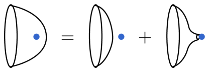
Figure 2: Skein-like relation for an M2-brane wrapping an embedded holomorphic disk: when crossing an M5-brane, the M2 breaks up and leaves behind a new curve with a new boundary on the M5.

3.1.2 Orbifold models of multiply wrapped disks

As discussed above, two-level holomorphic buildings where the inside (the part near the Lagrangian) is a punctured un-branched cover of a punctured disk and where the outside (the part far from the Lagrangian) is an embedded punctured sphere are key objects in our generalized quivers. In order to understand the behavior of such holomorphic objects, we can view them from inside and move the embedded sphere part far away. This means shrinking the outside punctured sphere together with the Reeb orbit where it is attached to a point and that gives an orbifold disk. In this section we study topological strings on orbifolds.

We start our discussion from the following identity, relating the partition function of a $\mu$-times around basic disk to $\mu$ once-around basic disks, with specific $B$-field fluxes:

$$(x^{\mu};q^{2\mu})_{\infty}^{-1}=\prod_{n\geq 0}(1-x^{\mu}q^{2\mu n})^{-1}=\prod_{k=0}^{\mu-1}\prod_{n\geq 0}(1-\zeta^{k}xq^{2n})^{-1}=\prod_{k=0}^{\mu-1}(\zeta^{k}x;q^{2})_{\infty}^{-1}\,,$$ (26)

where $\zeta$ is a primitive $\mu$-th root of unity. We will explain how such expressions appear from certain ‘fillings’ of cylindrical versions of punctured orbifold singularities. We start in the simplest non-trivial case, when $\mu=2$. Here we simply have

$$(x^{2};q^{4})_{\infty}=(x;q^{2})_{\infty}(-x;q^{2})_{\infty}\,.$$ (27)

This equation appears geometrically from the toric brane in $\mathcal{O}(0)\oplus\mathcal{O}(-2)\to{\mathbb{C}}{\mathbb{P}}^{1}$ in a certain limit. Consider the toric diagram in figure 3. The mirror curve is

$$F(x,y)=1-y-(1+Q)x+Qx^{2}\,,$$ (28)

with a single solution

$$y=(1-x)(1-Qx)\,.$$ (29)

In the limit $Q\to e^{\pi i}=-1$ (the complexified Kähler modulus is purely $B$-field) this becomes

$$1-y-x^{2}=0\,,$$ (30)

which is precisely the classical limit of (103) with $C_{ii}=0$.

Figure 3: Toric diagram of $\mathcal{O}(0)\oplus\mathcal{O}(-2)\to{\mathbb{C}}{\mathbb{P}}^{1}$.

Switching from the classical to the quantum level, we consider a toric brane on the horizontal leg. Its partition function can be evaluated by topological vertex techniques:

$$Z(x)=(x;q^{2})_{\infty}^{-1}(Qx;q^{2})_{\infty}^{-1}\,.$$ (31)

This is annihilated by the quantum curve

$$\hat{y}=(1-\hat{x})(1-Q\hat{x})\,,$$ (32)

whose classical limit recovers (29). Now an orbifold limit $Q\to-1$ turns the curve into

$$\hat{y}=(1-\hat{x})(1+\hat{x})=1-\hat{x}^{2}$$ (33)

and the partition function collapses to

$$Z(x)\to(x;q^{2})_{\infty}^{-1}(-x;q^{2})_{\infty}^{-1}=(x^{2};q^{4})_{\infty}^{-1}\,.$$ (34)

This is precisely the proposal for the unrefined partition function of a twice-around basic disk. Indeed,

$$(x^{2};q^{4})_{\infty}^{-1}=\sum_{k\geq 0}\frac{x^{2k}}{(q^{4};q^{4})_{k}}$$ (35)

matches with the form proposed in (64) with $C_{11}=0$, $\mu_{1}=2$ and $x_{1}=x^{2}$.

In order to see the geometry underlying these calculations, consider the orbifold $\mathbb{C}\times(\mathbb{C}^{2}/(\mathbb{Z}/2\mathbb{Z}))$ and remove the codimension four fixed point locus $\mathbb{C}\times[0]$, where $[0]$ denotes the point in the orbifold quotient which is the image of $0\in\mathbb{C}^{2}$. We view the resulting symplectic manifold as having a negative end (the negative half of the symplectization of standard contact $\mathbb{R}{\mathbb{P}}^{3}$ times $\mathbb{C}$) near the removed locus and note that there are two fillings: the orbifold itself and $\mathcal{O}(-2)\oplus\mathcal{O}(0)$. In the latter filling we view the symplectic area of the sphere as zero since the filling is at negative infinity. We can now interpret the limit $Q\to-1$ as this negative end splitting off from $\mathcal{O}(-2)\oplus\mathcal{O}(0)$. When this happens, punctured versions of the curves remain in the punctured orbifold and these can be completed by curves in the actual orbifold filling. As the flux through the sphere at negative infinity is set to $\pi i$, the partition functions match. Geometrically, this can be interpreted as the fact that upper level connected curves with odd asymptotics cancel, whereas those with even asymptotics add. This means that all non-zero curves can be filled with the orbifold end or the $\pi i$ flux $\mathcal{O}(-2)\oplus\mathcal{O}(0)$ and that the curve counts agree. Thus, from the viewpoint of curve counts in the two-level symplectic manifold, the two fillings give the same result. Moreover, as the filling $\mathcal{O}(-2)\oplus\mathcal{O}(0)$ moves toward negative infinity, the moduli space of curves in the upper level approaches the corresponding space for the orbifold. It is in this sense that taking the limit $Q\to-1$ should be understood.

Figure 4: Toric diagram of the resolution of the orbifold ${\mathbb{C}}\times({\mathbb{C}}^{2}/({\mathbb{Z}}/\mu{\mathbb{Z}}))$.

Higher degree basic disks appear in more complicated orbifold quotients. The corresponding toric diagram is shown in figure 4 and gives the mirror curve

$$y=(1-x)(1-Q_{1}x)\dots(1-Q_{\mu-1}x).$$ (36)

In analogy with the case $\mu=2$ above, we take the limit $Q_{k}\to e^{\frac{2\pi i}{\mu}k}$ and get the mirror curve of the orbifold $\mathbb{C}\times(\mathbb{C}^{2}/(\mathbb{Z}/\mu\mathbb{Z}))$.

$$1-y-x^{\mu}=0.$$ (37)

On the quantum level this reproduces the identity (26). The geometric interpretation is as above: we count two level curves in the two level symplectic manifold. The upper level of this manifold is the orbifold with the central $\mathbb{C}\times[0]$ removed, viewed as a symplectic manifold with an end given by the negative half of the symplectization of the standard contact lens space $L(\mu,1)$ times $\mathbb{C}$. The filling of the negative end is either the orbifold itself or the manifold given in figure 4 with zero-area spheres, since they live at negative infinity, and with $B$-field fluxes $\frac{2\pi}{\mu}k$ so that curve counts are identical. The convergence of moduli spaces works in direct analogy with the $\mu=2$ case.

3.1.3 Semiclassical consequences of basic disk denominators

It is worth noting that the difference between the standard denominators $(q^{2};q^{2})_{d_{i}}$ and $(q^{2\mu_{i}};q^{2\mu_{i}})_{d_{i}}$ we propose in (64) can be seen already at the semiclassical level. Consider a single basic $\mu$-times around disk with no self-linking. Then the partition function

$$P=\sum_{d\geq 0}\frac{x^{d\mu}}{(q^{2\mu};q^{2\mu})_{d}}=(x^{\mu};q^{2\mu})_{\infty}^{-1}$$ (38)

is annihilated by $1-\hat{y}-\hat{x}^{\mu}$, since

$$\hat{y}\cdot(x^{\mu};q^{2\mu})_{\infty}^{-1}=(q^{2\mu}x^{\mu};q^{2\mu})_{\infty}^{-1}=(1-x^{\mu})(x^{\mu};q^{2\mu})_{\infty}^{-1}\,.$$ (39)

The classical curve is therefore

$$1-x^{\mu}-y=0\,.$$ (40)

On the other hand, a partition function like

$$\tilde{P}=\sum_{d\geq 0}\frac{x^{d\mu}}{(q^{2};q^{2})_{d}}=(x^{\mu};q^{2})_{\infty}^{-1}$$ (41)

would behave as follows:

$$\hat{y}\cdot(x^{\mu};q^{2})_{\infty}^{-1}=(q^{2\mu}x^{\mu};q^{2})_{\infty}^{-1}=(1-x^{\mu})\dots(1-x^{\mu}q^{2\mu-2})(x^{\mu};q^{2\mu})_{\infty}^{-1}\,.$$ (42)

The classical curve in this case is quite different:

$$(1-x^{\mu})^{\mu}-y=0\,.$$ (43)

Therefore, in order to detect the difference between the two types of denominator, it is sufficient to compute the unrefined contributions from genus-zero basic curves to the augmentation polynomial. In section 6 we will provide concrete examples where the distinguished form of the curve (40) appears.

3.2 Holomorphic curves viewed as BPS generators

The structure of HOMFLY-PT homology seems to indicate that it is more closely related to the expansion of the refined partition function of the theory $T[L_{K}]$ in terms of equivariant vortices than to the corresponding expansion in terms of basic holomorphic curves. This means that in order to extract homology information from basic holomorphic curves viewed as BPS generators, we must understand how to expand a configuration of such objects as a combination of vortices. In this section we discuss a proposal for such an expansion and its origins. We study the expansions for single generators, first on the unrefined and then on the refined levels. The discussion here is in a sense localized near the boundary of the curve and independent of other charges, which on the unrefined level comes from homology class, 4-chain intersections, self-linking, and – on the refined level – also on a certain framing density term that we discuss in section 3.4.

Consider a basic holomorphic curve. As explained in section 3.1, such a curve consists of a punctured embedded sphere on the outside, asymptotic to a multiple of the unique Reeb orbit, and an unbranched multiple cover of the basic cylinder stretching from the simple Reeb orbit to the geodesic in the zero section on the inside.

In particular, our basic once-around disk becomes a two level building consisting of an outside sphere with puncture and an inside disk with puncture. The contribution to the partition function comes from multiple covers of this curve together with constant curves attached along it. Here we propose to push the contributions from the constants down to the boundary. We observe that at the level of generalized curves this can be done in a specific way: the contributions from constants correspond to very thin holomorphic annuli with one boundary component linking the basic curve and the other one not linking it. For a $d$-fold multiple cover of a basic disk, there is one such annulus on each level of magnification. The first annulus links all strands, the second all but one, etc., until the last annulus which links only one strand, see figure 5.

Figure 5: Contributions of pushed down constant annuli to generalized curve counts. Both boundaries of each annulus follow the longitude, one of the boundaries also wraps around a small meridian, linking with the boundary of the $i$-th strand. The overall holonomy is $y_{i}\cdot x\cdot x^{-1}=y_{i}$.

To support this picture, let us explain how it relates to the more familiar count of multiple covers of a single holomorphic disk with boundary on $L_{K}$. Recall that $L_{K}$ carries a $U(1)$ local system, with meridian and longitudinal holonomies at the boundary denoted $x,y$. These holonomies provide (exponentiated) Darboux coordinates for the moduli space of abelian flat connections on $T^{2}\simeq\partial L_{K}$. We denote their deformation quantization by $\hat{x},\hat{y}$, obeying the relation $\hat{y}\hat{x}=q^{2}\hat{x}\hat{y}$. Any disks ending on $L_{K}$ arise through the large $N$ geometric transition, descending from a common holomorphic cylinder stretching between the zero-section in $T^{*}S^{3}$ and $L_{K}$. As the boundaries of this cylinder are the original knot $K\subset S^{3}$ and the longitude in $L_{K}$, its skein valued partition function will be given by (8), where $P_{r}(K;a,q)$ is the HOMFLY-PT polynomial of $K$ in the $r$-th symmetric representation, and $x^{r}$ is the $U(1)$ HOMFLY-PT skein element in $L_{K}$ projected to homology and linking. For illustration, consider the unknot in reduced normalization, for which $P_{r}(0_{1};a,q)=1$. This gives the following partition function of a holomorphic disk

$$\psi(x)=P_{0_{1}}(x,a,q)=\sum_{r\geq 0}\frac{x^{r}}{(q^{2};q^{2})_{r}}=(x;q^{2})_{\infty}^{-1}$$ (44)

From the viewpoint of $U(1)$ Chern-Simons on $L_{K}$, boundaries of worldsheet instantons wrapping the holomorphic disk give rise to infinite series of Wilson lines Witten:1992fb . A Wilson line wrapping $r\geq 0$ times around $L_{K}$ with $k$ kinks on it contributes with $q^{2k}x^{r}$. The number of such Wilson lines is $c_{k,r}$, defined by the expansion

$$\psi(x)=\sum_{r\geq 0}\sum_{k\geq 0}c_{k,r}\,q^{2k}{x^{r}}\,.$$ (45)

The interpretation of $q^{2k}x^{r}$ as an $r$-times wrapped Wilson line with $k$ kinks can be seen by noting that kinks are counted by powers of $a$ as in figure 1, and by noting that in $U(1)$ Chern-Simons $a=q$. Incidentally, $c_{k,r}$ is also the dimension of the Hilbert space of BPS vortices of $T[L_{K}]$ with vorticity $r$ and spin $k$ Dimofte:2010tz .

Kinks on the boundary of a Wilson line can be traded with linking with a dual Wilson line using the $U(1)$ skein algebra of variables $\hat{x},\hat{y}$:

$$\frac{x^{r}}{(q^{2};q^{2})_{r}}=\,:\ \underbrace{\frac{1}{1-\hat{y}}\hat{x}\dots\frac{1}{1-\hat{y}}\hat{x}}_{r}\ :$$ (46)

where $:\ :$ is the normal ordering operation defined in Ekholm:2019lmb . Trading kinks with linking loops may be viewed as a ‘half’ of the $U(1)$ skein relation on $L_{K}$: the $\hat{x}$ Wilson line with a small $\hat{y}$ loop around it can be viewed as the over-crossing diagram in the first line of figure 1, while the kink corresponds to $q^{2}$ times the smoothing also on the first line.

Once again, this specific ensemble of Wilson lines can be given a geometric interpretation in terms of curve counting. The factor $\frac{1}{1-\hat{y}}$ corresponds to an annulus with a boundary linking the boundary of the $x$-cylinder in $L_{K}$ once, and with the other boundary linking zero times. Overall, the partition function resembles an $x$-annulus ending on $L_{K}$, with a linked $\hat{y}$-annulus on each strand of its multi-cover:

$$\psi(x)=\ :\ \sum_{r\geq 0}\left(\frac{1}{1-\hat{y}}\,\hat{x}\right)^{r}\ :\ =\ :\ \frac{1}{1-\frac{1}{1-\hat{y}}\,\hat{x}}\ :$$ (47)

The corresponding recursion relation is

$$\left(1-\left(\frac{1}{1-\hat{y}}\,\hat{x}\right)\right)\psi=1\,,$$ (48)

equivalent, upon left-multiplication by $1-\hat{y}$, to the more familiar

$$(1-\hat{y}-\hat{x})\psi=0\,.$$ (49)

As remarked above, a single vortex would contribute $q^{2k}x^{r}$ corresponding to a Wilson line. On the geometric side, we repackage Wilson lines into linked holomorphic annuli. On the gauge theory side of $T[L_{K}]$, this repackaging corresponds to the definition of equivariant vortices.

Given this, we now propose to think about an equivariant vortex in the theory $T[L_{K}]$ simply as a configuration of the form above: on level $d$, there are $d$ parallel copies of the central curve linked in the nested way by basic annuli, see figure 5.

We next consider the corresponding procedure applied to a $\mu$ times around generator. We propose that such generators become multiples of $\mu$ with constants and anti-constants attached on all intermediate covers. The constant and anti-constant push down to the boundary as almost identical annuli, where the second annulus has a twist in the trivialization on the boundary corresponding to $t$ or $t^{-1}$, depending on the underlying half-framing of the underlying punctured disk. Figure 6 shows the configuration for a twice-around generator.

Figure 6: A degree 2 generator with constants pushed down.

The configuration for a $\mu$ times around generator is clear and gives the refined contribution

$$:\frac{1}{{1+t^{\pm 1}\hat{y}}}\left(\frac{1+t^{\pm 1}\hat{y}}{1-\hat{y}}\hat{x}\right)^{\mu}:.$$ (50)

The recursion relation for the refined partition function of a $\mu$-times around generator is then

$$\left(1-\frac{1}{{1+t^{\pm 1}\hat{y}}}\left(\frac{1+t^{\pm 1}\hat{y}}{1-\hat{y}}\hat{x}\right)^{\mu}\right)\psi=1.$$ (51)

To illustrate the procedure, we next consider the second level of a system of two unlinked basic disks. We must express the configuration of two strands with an annulus linking each in terms of our standard basis, which leads to the counting of intersections presented in figure 7.

Figure 7: Contributions on second level from two unlinked basic disks.

We next look at this way of expanding states in terms of vortices and their Hilbert spaces. Consider an equivariant vortex. Its partition function is given by

$$\psi(x,q)=\sum_{d\geq 0}\frac{x^{d}}{(1-q^{2})\dots(1-q^{2d})}.$$ (52)

Expanding the denominators using geometric series, it is convenient to think of the Hilbert space at level $d$ as follows. Consider the points in the simplex $x_{1}\geq x_{2}\geq\dots x_{d}\geq 0$ with integer coordinates $(n_{1},\dots,n_{d})$. The dimension of the Hilbert space of states with $q$-charge $k$ is then the number of points in the intersection between the simplex and the plane $\sum_{j=1}^{d}x_{j}=k$.

The Hilbert space of mixed states of two vortices on level two as above looks like the integral points over the first quadrant and can be expressed as two copies of the simplex, one shifted by multiplication by $q^{2}$. Similarly, one generator going $\mu$ times around corresponds to the points along the diagonal $x_{1}=\dots=x_{\mu}$ and can be expressed as a sum of shifted simplices. This indicates that refinement applies to the Hilbert spaces associated to vortices individually.

We give one final perspective on vortices and homology. Viewing a vortex as an $U(1)$-invariant fixed point in $\mathbb{C}$, we may compute its contribution to the partition function by Bott localization. Here we change coordinates and think of the $d$-fold vortex as a point in the configuration space of $d$ points in $\mathbb{C}$ thought of as the space of polynomials using the relation between roots an coeffcients. The contribution

$$\frac{1}{(1-q^{2})\dots(1-q^{2d})}$$ (53)

now arises as the equivariant Chern character. For a $\mu$ times around generator, only the top degree coefficients of the polynomials are fixed, others are free to vary. This means we have a corresponding $\mathbb{C}^{\mu-1}$ family of fixed points with similar action on normal bundles. The contribution from the corresponding Bott manifold is

$$\frac{1}{(1-q^{2d})}\cdot[(\mathbb{C}{\mathbb{P}}^{1})^{d-1}],$$ (54)

where we have replaced $\mathbb{C}$ with $\mathbb{C}{\mathbb{P}}^{1}$ and a fixed point also at infinity and where when we pass from Bott to Morse we get the contribution

$$\frac{1+tq^{2}}{1-q^{2}}\dots\frac{1+tq^{2(\mu-1)}}{1-q^{2(\mu-1)}}\frac{1}{1-q^{2d}},$$ (55)

corresponding to two fixed points in each $\mathbb{C}{\mathbb{P}}^{1}$-factor.

3.3 M2-branes wrapping holomorphic curves

In this section we discuss the physical and geometric interpretations of refinement, connecting the conjectures of Aganagic:2011sg to our interpretation of the knot-quiver correspondence Ekholm:2018eee ; Ekholm:2019lmb . The 3d ${\mathcal{N}}=2$ index (20), proposed by Aganagic:2011sg , corresponds to the refined partition function of knot invariants. However, this index is well-defined if not just one, but two supercharges are preserved in the Omega-background and with an M5-brane inserted along $L\times S^{1}\times{\mathbb{R}}^{2}$. We will now provide motivation for the existence of this additional supercharge, based on the presence of a certain geometric $U(1)$ symmetry, expanding on a suggestion of Aganagic:2011sg . Eventually, this will lead us to a geometric interpretation of the R-charges of BPS states in terms of ‘self-linking densities’, consistent with our previous observations in Ekholm:2018eee . Then, together with the study in section 3.2, this gives our generalized quiver partition function.

The analysis of preserved supersymmetries that we develop here takes a different perspective from the one in section 2.4. There we started with supercharges of the 5d theory engineered by $X$ and examined which ones survive in presence of the Omega-background, and eventually also in presence of the M5-brane on $L\times S^{1}\times{\mathbb{R}}^{2}$. Here we shall start with the worldvolume supersymmetry on the M5 and analyze how it is broken by introducing the Calabi-Yau background and by placing the brane on $L$. An interesting novelty of this perspective is that it will clarify a little-appreciated consequence of the $U(1)$ symmetry postulated in Aganagic:2011sg . As we will show, the existence of a $U(1)$ symmetry corresponds to a point in the moduli space of $T[L]$ with enhanced supersymmetry.

3.3.1 Conserved supercharges in the generic case

We study M-theory on the resolved conifold $X=\mathcal{O}(-1)\oplus\mathcal{O}(-1)\to{\mathbb{C}}{\mathbb{P}}^{1}$ times $S^{1}\times{\mathbb{R}}^{4}$, with an Omega-deformation turned on. This consists of rotations of the planes ${\mathbb{R}}^{2}\times{\mathbb{R}}^{2}$ by independent phases $\epsilon_{1,2}$ when going around the $S^{1}$ Nekrasov:2002qd ; Nekrasov:2003rj .

The Calabi-Yau background preserves eight supercharges. This amount of supersymmetry is further reduced if we consider an M5-brane wrapped on a special Lagrangian submanifold $L\subset X$ times $S^{1}\times{\mathbb{R}}^{2}_{\epsilon_{1}}$. Recall that a special Lagrangian is a Lagrangian calibrated by the holomorphic top form on $X$, which must have a constant phase along $L$, the phase determines which supercharges are preserved and which are broken by the M5-brane. Under a genericity assumption, such a configuration preserves four supercharges. Let us review how this works.

In a flat space the theory on an M5-brane would be the abelian 6d (2,0) SCFT, with 16 supercharges transforming as $({\bf 4,4})$ spinors under $Spin(1,5)\times Spin(5)$, with the second factor corresponding the R-symmetry group. With the Calabi-Yau background, the latter is broken to $Spin(3)\times Spin(2)$, where $Spin(3)$ is a subgroup of the local rotations on $X$ which leave $L$ fixed, and $Spin(2)\simeq U(1)_{2}$ is the group of rotations of ${\mathbb{R}}^{2}_{\epsilon_{2}}$. The (2,0) 6d supercharges thus decompose as follows:

$$({\bf 4;4})\to({\bf 2,2;2})_{+1/2}\oplus({\bf 2,2;2})_{-1/2}$$ (56)

as representations of

$$\underbrace{Spin(3)_{TL}\times Spin(1,2)_{S^{1}\times{\mathbb{R}}^{2}_{\epsilon_{1}}}}_{\subset Spin(1,5)}\times\underbrace{Spin(3)_{NL}\times Spin(2)_{{\mathbb{R}}^{2}_{\epsilon_{2}}}}_{{\subset Spin(5)}}\,.$$ (57)

The holonomy on $X$ belongs to an $SU(3)\subset SU(4)\simeq Spin(6)$ subgroup. This induces nontrivial holonomies for both $Spin(3)_{TL}$ and $Spin(3)_{NL}$, further reducing the number of conserved supercharges. The special Lagrangian property of $L$ implies that holonomies of the tangent and normal directions to $L$ are related. This means that to any given loop $\gamma\in\pi_{1}(L)$ one may associate holonomies for both $NL$ and $TL$, denoted respectively $g_{TL}\in Spin(3)_{TL}$ and $g_{NL}\in Spin(3)_{NL}$. Due to the fact that $L$ is a special Lagrangian of $X$, these group elements are in fact related to each other, allowing one to perform a topological twist by considering the diagonal subgroup $Spin(3)_{dL}\subset Spin(3)_{TL}\times Spin(3)_{NL}$. Then, spinors in the $({\bf 2,2})$ transform as ${\bf 2\otimes 2=1\oplus 3}$, implying that one out of four components is invariant under holonomy. This leaves four conserved supercharges, which transform as

$$({\bf 1,2})_{+1/2}\oplus({\bf 1,2})_{-1/2}\quad\text{under}\quad Spin(3)_{dL}\times Spin(1,2)_{S^{1}\times{\mathbb{R}}^{2}_{\epsilon_{1}}}\times Spin(2)_{{\mathbb{R}}^{2}_{\epsilon_{2}}}\,.$$ (58)

These are the four supercharges of 3d ${\mathcal{N}}=2$ theory $T[L]$ arising on the M5-brane worldvolume, along directions $S^{1}\times{\mathbb{R}}^{2}_{\epsilon_{1}}$. This amount of supersymmetry can be preserved under generic conditions under our assumptions, namely for an M5-brane wrapping any special Lagrangian $L$ in any Calabi-Yau threefold $X$.

3.3.2 Supersymmetry enhancement from a geometric $U(1)$-symmetry

Following Aganagic:2011sg , the definition of a refined index requires an additional supercharge in addition to those in (58). In view of this we make the following assumption.

Assumption 3.3.

The Lagrangian $L$ is diffeomorphic to $S^{1}\times{\mathbb{R}}^{2}$ and there exists a $U(1)$-action on $L$ which rotates the $S^{1}$-factor. The corresponding vector field $V$ defines a normal plane ${\mathbb{R}}^{2}_{V}$ at each point. Then $\partial{\mathbb{R}}^{2}_{V}$ is the contractible meridian on the torus $\partial L$.

The embedding $TL\subset TX$ defines a dual vector field $JV$ normal to $L$ ($J$ is the complex structure on $X$). We view $JV$ as the direction in which an M2-brane wrapping a holomorphic curve in $X$ attaches to $L$. (If the M2 boundary lies along a flow line of $V$ in $TL$, and the M2 wraps a holomorphic curve in $X$, its normal is tangent to a flow line of $JV$ in $J\cdot TL\simeq NL$, using the local splitting $TX\simeq TL\oplus NL$.) Let ${\mathbb{R}}^{2}_{NL}$ be the family of planes normal to $JV$ within $NL$. Now we come to the assumption: the existence of a $U(1)$-action implies that the holonomy $g_{TL}\in Spin(3)_{TL}$ is actually not generic, but belongs to a subgroup $Spin(2)_{V}$ that rotates the planes ${\mathbb{R}}^{2}_{TL}$ tangent to ${\mathbb{R}}^{2}_{V}$ as one goes around $S^{1}$ corresponding to the boundary of a holomorphic curve. Since $L$ is special Lagrangian, $g_{TL}=g_{NL}$ and therefore the holonomy induces a rotation of ${\mathbb{R}}^{2}_{NL}$. The holonomy $g_{V}=g_{TL}=g_{NL}\in Spin(2)_{dL}\subset Spin(3)_{dL}$, so it rotates both summands in ${\mathbb{R}}^{2}_{TL}\oplus{\mathbb{R}}^{2}_{NL}$ by the same amount, leaving fixed the ‘origin’ $S^{1}\times{\mathbb{R}}\subset TL\times NL$, corresponding to the tangent and normal directions of a holomorphic curve wrapped by M2 attaching to $L$.

Our proposal is to identify $U(1)_{I}\equiv Spin(2)_{NL}$ as the R-symmetry of the 5d theory $T_{5d}[X]$ that is necessary to perform a topological twist to preserve additional supercharges leading to a refined index, recall the discussion from section 2.4. We will elaborate on the details shortly.

First, we wish to stress that $U(1)_{I}$ is an artifact of the string theory setup, and not a property of a garden-variety 3d ${\mathcal{N}}=2$ theory. On the one hand, while surviving 3d ${\mathcal{N}}=2$ spinors are invariant under $Spin(2)_{dL}$, they transform nontrivially under $U(1)_{I}$. On the other hand, $U(1)_{I}$ is not an automorphism of the 3d ${\mathcal{N}}=2$ super-Poincaré algebra, i.e., it is not an R-symmetry of the 3d theory. To establish these claims, recall that surviving spinors arise from the branching rule ${\bf 2\otimes 2=1\oplus 3}$ for $Spin(3)_{dL}\subset Spin(3)_{TL}\times Spin(3)_{NL}$. Also recall that, following the above assumption, we identified a distinguished $Spin(2)_{TL}\times Spin(2)_{NL}\subset Spin(3)_{TL}\times Spin(3)_{NL}$, whose generators will be denoted $J^{3}_{TL},J^{3}_{NL}$. Working in a basis where $J^{3}_{TL},J^{3}_{NL}$ are diagonal, we may reclassify the spinors in (56) as follows:

$$({\bf 4;4})\to(\pm 1/2,{\bf 2};\pm 1/2)_{+1/2}\oplus(\pm 1/2,{\bf 2};\pm 1/2)_{-1/2}$$ (59)

as representations of of the following subgroup of (57)

$$Spin(2)_{TL}\times Spin(1,2)_{S^{1}\times{\mathbb{R}}^{2}_{\epsilon_{1}}}\times Spin(2)_{NL}\times Spin(2)_{{\mathbb{R}}^{2}_{\epsilon_{2}}}\,.$$ (60)

Topological twisting with reduced holonomy $Spin(2)_{TL}\times Spin(2)_{NL}$ implies retaining those supercharges that are invariant under the diagonal subgroup. In this case, these are the ones with opposite charges $j_{V}=-j_{JV}$ under $Spin(2)_{TL}\times Spin(2)_{NL}$:

$$(\pm 1/2,{\bf 2};\mp 1/2)_{+1/2}\oplus(\pm 1/2,{\bf 2};\mp 1/2)_{-1/2}\,.$$ (61)

This leaves a total of four plus four conserved supercharges, twice the generic amount in (58). To lighten notation, we will sometimes omit the representation labels under $Spin(1,2)_{S^{1}\times{\mathbb{R}}^{2}_{\epsilon_{1}}}\times Spin(2)_{{\mathbb{R}}^{2}_{\epsilon_{2}}}$, and simply use $(j_{V},j_{JV})$.

Among these, we can recognize the singlet ${\bf 1}$ that survived in the general case (58). This must be a linear combination proportional to $(1/2,-1/2)-(-1/2,1/2)$, since it arose as the second anti-symmetric power of ${\bf 2}$ for the diagonal subgroup $Spin(3)_{dL}$. Overall, there are four supercharges in the singlet: a ${\bf 2}$ of $Spin(1,2)$ with $j_{2}=+1/2$ and another with $j_{2}=-1/2$. There is also a second combination of supercharges that is conserved, namely $(1/2,-1/2)+(-1/2,1/2)$. While this is part of the triplet ${\bf 3}$ and therefore not invariant under the generic $Spin(3)_{dL}$, it is nonetheless invariant under the reduced $Spin(2)_{dL}$. Again, this corresponds to four supercharges. Therefore, our assumptions on the geometry of $L$ and the existence of a $U(1)$-action imply doubling the supersymmetry from 3d ${\mathcal{N}}=2$ in the generic setting to 3d ${\mathcal{N}}=4$ in presence of $U(1)$.

For Lagrangians $L=S^{1}\times\mathbb{R}^{2}$ as above this has the following consequences. From the point of view of the theory $T[L]$ in the generic case, without the additional $U(1)$-symmetry, the Hilbert space of states is generated by vortices and contains states of fixed vorticity $x^{r}$ and fixed spin in the $\mathbb{R}^{2}_{\epsilon_{1}}$-plane, $q^{2s}$. The partition function is a (super)trace which for fixed vorticity $x^{r}$ gives a Laurent series in $q^{2}$. As the state space is generated by vortices, the coefficients stabilize as the power of $q^{2}$ goes to infinity, and the coefficient of $x^{r}$ can be expressed as $P_{r}(q^{\pm 2})(q^{2};q^{2})_{r}^{-1}$, where $P_{r}$ is a polynomial with integer coefficients. With additional $U(1)$-symmetry, there is an additional $t$-charge that refines this theory and its states. The Hilbert space is now a sum of finite dimensional vector spaces of fixed charges $x^{r}q^{2s}t^{l}$. As before, after fixing the vorticity $x^{r}$ the Poincaré polynomial of the vector spaces stabilizes and we can write it as $\mathcal{P}_{r}(q^{\pm 2},t^{\pm 1})(q^{2};q^{2})_{r}^{-1}$, where $\mathcal{P}_{r}$ is a polynomial with positive integer coefficients and such that $\mathcal{P}_{r}(q^{\pm 2},-1)=P_{r}(q^{\pm 2})$.

3.3.3 Omega-background and 3d index

Now we come back to the definition a refined 3d index (20). First we note that, while surviving supercharges are not neutral under $Spin(2)_{NL}$, neither do they transform in a representation of $Spin(2)_{NL}$. In this sense $U(1)_{I}$ is not a symmetry of the 3d ${\mathcal{N}}=2$ superalgebra. For this reason we consider linear combinations of the two conserved supercharges. In particular, one may view $(1/2,-1/2)$ and $(-1/2,1/2)$ as being separately conserved. With this change of basis, supercharges transform as representations of $U(1)_{I}$: the first batch with charge $-1/2$, the second batch with charge $+1/2$. Overall, the surviving supercharges are $({\bf 2})_{j_{V},j_{2}}$, where $j_{V}=-j_{JV}$ and $j_{V},j_{2}\in\{-1/2,+1/2\}$ are chosen independently. Note that $j_{I}\equiv j_{JV}=-j_{V}$ is the charge under $U(1)_{I}$.

The point of having supercharges with a well-defined charge under $U(1)_{I}$ is that one can turn on the Omega-background and use the $U(1)_{I}$ remnant of the 5d R-symmetry to perform a topological twist. The Omega-background means that as we go around the M-theory circle, we perform a rotation of $U(1)_{1}\times U(1)_{2}\times U(1)_{I}$. In particular, this breaks $Spin(1,2)_{S^{1}\times{\mathbb{R}}^{2}}$ to $U(1)_{1}$ and spinors $({\bf 2})_{j_{V},j_{2}}$ get labeled by their $U(1)$ charges $(j_{1},j_{2},j_{I})$. In this notation, the surviving supercharges are those with $j_{1}=j_{2}=-j_{I}$, as derived in (16). This can be shown to match precisely with the supercharges considered in Aganagic:2011sg .

3.4 R-charge, homological degree, and self-linking

We summarize the geometry near the Lagrangian considered above. The Lagrangian itself is $S^{1}\times\mathbb{R}^{2}$ and a neighborhood of it in the Calabi-Yau looks like its cotangent bundle $T^{\ast}(S^{1}\times{\mathbb{R}}^{2})$. We furthermore have a $U(1)$-action that rotates the $S^{1}$-direction, and which splits the normal bundle of the Lagrangian as $NL=\mathbb{R}\times{\mathbb{R}}^{2}_{NL}$. We can therefore write a neighborhood of the locus of the M5-brane as

$$(S^{1}\times{\mathbb{R}})\times({\mathbb{R}}^{2}_{TL}\times\mathbb{R}^{2}_{NL})\times{\mathbb{R}}^{2}_{q}\times{\mathbb{R}}^{2}_{q^{-1}t}\times S^{1},$$ (62)

where normal directions lie in ${\mathbb{R}}\times{\mathbb{R}}^{2}_{NL}\times{\mathbb{R}}^{2}_{q^{-1}t}$. Here ${\mathbb{R}}^{2}_{q}$ and ${\mathbb{R}}^{2}_{q^{-1}t}$ come from (21): they are the planes that are rotated by $J_{1}$ and $J_{2}$, respectively. The topological twist reduces the structure group of this bundle to a diagonal $U(1)$ rotating both factors ${\mathbb{R}}^{2}_{NL}\times{\mathbb{R}}^{2}_{q^{-1}t}$ in the same way.

3.4.1 Once-wrapped disks

We next read off the $t$-charge of an M2-brane wrapped on $(S^{1}\times{\mathbb{R}})\times S^{1}$. In the Calabi-Yau space this is a holomorphic curve along $S^{1}\times{\mathbb{R}}$. By holomorphicity, its normal variation along the boundary is given by a vector field $(v,Jv)\in{\mathbb{R}}^{2}_{TL}\times{\mathbb{R}}^{2}_{NL}$. This implies that, going around a loop in $S^{1}$, the vector field $v$ rotates in ${\mathbb{R}}^{2}_{TL}$ by an amount that equals that of $Jv$ in ${\mathbb{R}}^{2}_{NL}$. The former furthermore equals the self-linking $C_{ii}$ in $L$. By the topological twist the rotation of $Jv$ contributes to the $t$-degree and it follows that the corresponding $t$-charge of a $d$-fold cover is $q^{-C_{ii}d}(-t)^{C_{ii}d}$, in line with the conjectural identification of $C_{ii}$ and the homological $t$-degree Kucharski:2017poe ; Kucharski:2017ogk .

We point out that the origin of the contribution $q^{C_{ii}d^{2}}$ to the partition function is different: it comes from counting $q$-power in the $U(1)$-skein and then passing to homology and (self-)linking. In other words, the quadratic growth of powers of $q$ corresponds to the contribution to the Gromov-Witten invariant from counting generalized holomorphic curves. In physics this corresponds to the open topological string partition function with an $A$-brane on $L$, where $q$ arises through the M-theory interpretation of the string coupling constant Ooguri:1999bv . There are $C_{ii}$ crossings between $d$-fold covers of an underlying once-around curve which gives $q^{C_{ii}d^{2}}$. Overall we have contribution $q^{C_{ii}d^{2}-C_{ii}d}(-t)^{C_{ii}d}$ for the $d$-fold cover of a once-around disk. We stress that this reasoning is based on a picture of M2-branes wrapping $d$ times around, viewed as tightly packed copies of an underlying once-around disk.

Our prescription should recover the contribution to the unrefined partition function in the limit $t=-1$. On this level we should perturb multi-covers of the underlying curve and then count generalized curves. The geometry behind the count is the following. A contribution to $C_{ii}$ can be thought of as an infinitesimal kink. After perturbation we find an actual kink with $d^{2}$ crossings; in order for this to be $d$ times a curve in framing $C_{ii}$, we deform to make all innermost kinks very small and then pull them out, making them infinitesimal again and trading them for framing. This leaves $d(d-1)$ crossings, and summing contributions from all $C_{ii}$ infinitesimal twists we eventually get $q^{C_{ii}d(d-1)}$. This agrees with the specialization to $t=-1$.

Remark 3.4.

To round off our discussion on the geometric interpretation of the homological degree of BPS states, we offer yet another reason why such geometric information (the ‘wiggling’ of an M2-brane boundary) should play a role in the definition of the BPS partition function. M2-branes wrapping holomorphic curves produce Wilson lines for the $U(1)$ Chern-Simons theory on $L$. From the viewpoint of the full 6d ${\mathcal{N}}=$(2,0) theory describing the worldvolume dynamics of a single M5-brane, such Wilson lines correspond to reduction of Wilson surfaces. By supersymmetry, these involve integration along the boundary of the M2 of the abelian 2-form connection, as well as the five scalars. In particular, the latter transform as a vector under the $Spin$(5) R-symmetry of the (2,0) theory. Recalling that R-symmetry corresponds to rotations transverse to the brane, the winding number of these scalars around the brane must correspond to their charge under R-symmetry. At the same time, the scalars parametrize embeddings of M5 in the transverse directions, and in particular they parametrize the direction along which the M2 ends on M5. Yet again, this suggests that the wiggling of the M2 boundary is captured by the R-charge of a BPS state, which in the setup involving $L\subset X$ is eventually identified with the homological degree.

3.4.2 Multiply-wrapped disks

Our suggestion for refinement for multiply wrapped disks have two sources. The first arises when we express the contribution of the curve in terms of standard vortices, or geometrically in terms of a specific link as described in section 3.2. Here, internal $t$-charge of the M2-brane is transferred to thin annuli and appears as a difference in framing along their two boundary components. The second comes from an external framing analogous to the framing of the standard basic disks discussed above.

To describe this external $t$-degree, we refer to section 3.1.2 where multiply wrapped disks are related to disks in orbifolds and consider an M2-brane wrapped on a disk in a degree $\mu$ orbifold corresponding to (37). The $t$-charge arises from the $U(1)$-action on $L$, and the M2-brane is invariant under this action (rotation along $S^{1}$) only if its boundary remains a tightly wrapped $\mu$-fold cover of $S^{1}\times\text{point}$. This means that its boundary gives a single Wilson line of charge $\mu$ rather than a $\mu$-times around Wilson line of charge $1$. As in section 3.4.1, by holomorphicity and the topological twist that identifies rotations in ${\mathbb{R}}_{NL}$ and ${\mathbb{R}}^{2}_{q^{-1}t}$, the $t$-degree is the framing of this charge-$\mu$ Wilson line, which in turn is determined by its self-linking. We define $C_{ii}$ to be the framing density along the $\mu_{i}$-fold boundary of the M2-brane, thus $C_{ii}\in\frac{1}{\mu_{i}}\mathbb{Z}$. This means that a single twist of the underlying simple curve corresponds to $C_{ii}=\frac{1}{\mu_{i}}$. The total twist in the normal bundle is then $C_{ii}\mu_{i}\in{\mathbb{Z}}$, which leads to the charge $x_{i}^{d}\sim q^{-C_{ii}\mu_{i}d}(-t)^{C_{ii}\mu_{i}d}$ for a $d$-fold cover of the $\mu$-wrapped M2-brane. Next we consider the self-linking contribution to $q$-degree for generalized curves invariant under the covering transformation. We think of the framing $C_{ii}\mu_{i}$ of the underlying curve as a collection of infinitesimal kinks. These lift to $C_{ii}\mu_{i}^{2}$ kinks, giving the total contribution to the $q$-degree $q^{C_{ii}\mu_{i}^{2}d^{2}}$ at the $d$-fold level of the brane. In summary we then have contributions proportional to $q^{C_{ii}\mu_{i}^{2}d^{2}-C_{ii}\mu_{i}d}(-t)^{C_{ii}\mu_{i}d}$ at the $d$-fold covering level.

Similarly to the once-around case, we consider the $t=-1$ specialization of this formula and the contribution to generalized curves after perturbation. As above we consider the lift to the $d$-fold cover. A $\mu_{i}$-wrapped curve with $C_{ii}\mu_{i}^{2}$ infinitesimal kinks gives $C_{ii}\mu_{i}^{2}d^{2}$ crossings at the $d$-fold covering level, after perturbation. In order to lift a curve $d$ times around a curve with framing $C_{ii}\mu_{i}$, we trade the innermost kinks at $C_{ii}\mu_{i}$ of the crossings for framing, leaving a net $C_{ii}\mu_{i}^{2}d^{2}-C_{ii}\mu_{i}d$ crossings and hence an overall contribution of $q^{C_{ii}\mu_{i}d(\mu_{i}d-1)}$.

We next consider a degree $\mu_{i}$ basic disk on a more general Lagrangian of topology $S^{1}\times\mathbb{R}^{2}$. Here, as before, we get a $U(1)$-symmetric boundary of the disk by SFT-stretching. In the limit where the embedded disk is split off, the lower piece close to the Lagrangian can be identified with the complement of the orbifold point in an orbifold disk. The addition of the orbifold point corresponds to adding the embedded disk ‘at infinity’. Again, the existence of a $U(1)$-action on $L$ implies that all boundaries of holomorphic curves should sit very close to each other, within an infinitesimal neighborhood of the orbits $S^{1}\times\text{point}$. The $t$-degree is then obtained from the framing of the once-around charge-$\mu$ boundary in the plane field normal to the orbits, and the contribution to the refined partition function at level $d$ is $(-t)^{C_{ii}\mu_{i}d}q^{C_{ii}\mu_{i}^{2}d^{2}-C_{ii}\mu_{i}d}$, exactly as above.

3.5 Multiply-wrapped basic disks and generalized quiver partition functions

In this section we collect the results of the arguments in section 3.4 and define a partition function for generalized quivers.

A generalized quiver $Q$ is an oriented graph with a finite number of vertices connected by finitely many signed arrows (signed oriented edges). We denote the set of vertices by $Q_{0}$ and the set of arrows by $Q_{1}$. A dimension vector for $Q$ is a vector in the integral lattice with basis $Q_{0}$, $\boldsymbol{d}\in{\mathbb{Z}}Q_{0}$. We number the vertices of $Q$ by $1,2,\dots,m=|Q_{0}|$. Each vertex $i$ has a positive integral multiplicity $\mu_{i}$. The adjacency matrix of $Q$ is the $m\times m$ rational matrix with entries $C_{ij}$ defined as follows. Let $N_{ij}\in\mathbb{Z}$ denote the number of signed arrows from $i$ to $j$. Then

$$C_{ij}=\begin{cases}N_{ij}&\text{ if }\mu_{i}\neq\mu_{j},\\ \frac{1}{\mu}\cdot N_{ij}&\text{ if }\mu_{i}=\mu_{j}=\mu.\end{cases}$$ (63)

A generalized quiver is symmetric if its adjacency matrix is.

Let $Q$ be a generalized quiver with nodes $1,2,\dots,m$ of multiplicities $\mu_{1},\dots,\mu_{m}$ and adjacency matrix $C_{ij}$. We associate variables $x_{i}$ to the generalized quiver nodes $i$ and define two partition functions as follows.

Definition 3.5.

The partition function of $Q$ is

$${P_{Q}(\boldsymbol{x};q)=\sum_{\boldsymbol{d}}(-1)^{\sum_{i}C_{ii}\mu_{i}d_{i}}q^{\sum_{i,j}C_{ij}(\mu_{i}d_{i})(\mu_{j}d_{j})}\prod_{i=1}^{|Q_{0}|}\frac{x_{i}^{d_{i}}}{(q^{2\mu_{i}};q^{2\mu_{i}})_{d_{i}}}}\,,$$ (64)

and the refined partition function of $Q$ is

$${P_{Q,t}(\boldsymbol{x};q)=\sum_{\boldsymbol{d}}(-1)^{\sum_{i}C_{ii}\mu_{i}d_{i}}q^{\sum_{i,j}C_{ij}(\mu_{i}d_{i})(\mu_{j}d_{j})}\prod_{i=1}^{|Q_{0}|}\frac{x_{i}^{d_{i}}}{(q^{2};q^{2})_{\mu_{i}d_{i}}}\frac{(-q^{2}t^{\sigma_{i}};q^{2})_{d_{i}\mu_{i}}}{(-q^{2\mu_{i}}t^{\sigma_{i}};q^{2\mu_{i}})_{d_{i}}}}\,,$$ (65)

where $\boldsymbol{d}$ ranges over all dimension vectors and where $\sigma_{i}=\pm 1$.

Note that $P_{Q,t=-1}(\boldsymbol{x};q)=P_{Q}(\boldsymbol{x};q)$ and all exponents of $q$ and $t$ appearing in the formulas are integers.

Definition 3.5 is the starting point for our main conjecture on HOMFLY-PT homology. Consider a knot $K$ and its conormal $L_{K}$ in the resolved conifold. We conjecture that it (after degeneration onto the unknot conormal) admits a $U(1)$-symmetry and that there is a finite number of basic disks that we label $1,\dots,m$. We view these disks as generalized quiver nodes, where the multiplicity of a node is the multiplicity of the boundary of the corresponding basic disk. Attaching data for the normal bundles of the basic disks give a quiver adjacency matrix $C_{ij}$. Here, for $i\neq j$, $C_{ij}$ is the infinitesimal mutual linking (a relative framing). In particular $C_{ij}$ is integral if $\mu_{i}\neq\mu_{j}$. For $\mu_{i}=\mu_{j}=\mu$, $C_{ij}$ is $\frac{1}{\mu}\cdot N_{ij}$, where $N_{ij}$ is the self- or mutual-linking, depending on whether $i=j$ or $i\neq j$. This defines a symmetric generalized quiver $Q$ associated to $K$. Let $\log x$ be the positive generator of $H_{1}(L_{K})$ and let $\log a^{2}$ denote homology class of $\mathbb{CP}^{1}$ in the resolved conifold. Let the homology class of the generalized disk $i$ be $\mu_{i}\log x+a_{i}\log a$ and its invariant self-linking (or 4-chain intersectiond far from the boundary) be $q_{i}$.

Conjecture 3.6.

If we substitute

$$x_{i}=x^{\mu_{i}}q^{q_{i}-C_{ii}\mu_{i}}a^{a_{i}}(-t)^{C_{ii}\mu_{i}},$$ (66)

for $i=1,2,\dots,m$, then the following hold.

• The generalized quiver partition function $P_{Q}(\boldsymbol{x};q)=P_{Q,t=-1}(\boldsymbol{x};q)$ equals the generating function of the Gromov-Witten invariants counting generalized holomorphic curves, or equivalently the generating function of the symmetrically colored HOMFLY-PT polynomials of $K$.

• The refined generalized quiver partition function $P_{Q,t}(\boldsymbol{x};q)$ equals the generating function of Poincaré polynomials of HOMFLY-PT homology in the symmetric represtentions.

Remark 3.7.

The powers $\sigma_{i}=\pm 1$ in the refined partition function are interpreted as follows: view the $\mu_{i}$ of the boundary of the generator $x_{i}$ as strands of a braid over the underlying once-around curve; we obtain a connected $\mu_{i}$-times around loop by gluing the endpoint of the last strand to the beginning of the first one, and this can be done passing above $\sigma_{i}=+1$ or below $\sigma_{i}=-1$ all other intermediate strands, according to the half framing of the attaching data of the neighborhood of the basic disk.

Remark 3.8.

The change of framing operation, counterpart to changing variables $x\to x(-y)^{f}$ with $f\in{\mathbb{Z}}$ in the augmentation curve, is given by the usual shift of the linking matrix $C_{ij}\to C_{ij}+f$, both for diagonal and off-diagonal elements, in the partition function.

Remark 3.9.

Equation (65) completes and corrects (Ekholm:2018eee, , Conjecture 1.1) as follows. There, a $d$ times around generator in framing zero was assumed to be an embedded disk that contributes $(x^{d};q^{2})_{\infty}$ to the partition function. Its contribution to the refined partition function was not specified as can be seen already on level $d$. To do so, one would have to explain how to express the current denominator $(q^{2};q^{2})_{1}$ in terms of $(q^{2};q^{2})_{d}$. Here the basic object is different: it is an embedded disk outside completed by a multiply covered disk inside. It contributes $(x^{d};q^{2d})_{\infty}$ to the partition function and on the refined level its denominators are corrected to $(q^{2};q^{2})_{kd}$ in (64).

Equations (64) and (65) differ from the proposed knots-quivers correspondence of Kucharski:2017ogk ; Kucharski:2017poe in several ways. They are not quiver partition functions, nor are they characters of a cohomological Hall algebra Kontsevich:2008fj ; 2011arXiv1103.2736E . Nevertheless, both expressions reflect the idea that the whole spectrum of BPS states is generated by a finite set of basic objects, interacting in a certain way. The basic objects may be viewed as nodes of a ‘generalized quiver’, whose adjacency matrix encodes their interactions. The main difference with the knots-quivers correspondence is that we allow for nodes with $\mu>1$ and with new denominators.

We list some arguments that show that some properties of our proposed partition function are necessary:

1. In any quiver-like description, nodes with $\mu>1$ are necessary, see Ekholm:2018eee and the examples in section 6.

2. A basic disk wrapping $\mu$-times around $L_{K}$ contributes to the multi-cover formula with $q^{2}$ replaced by $q^{2\mu}$. See section 3.1 for motivation and section 6 for examples. This leads to replacing denominators $(q^{2};q^{2})_{d_{i}}$ in (6) by $(q^{2\mu_{i}},q^{2\mu_{i}})_{d_{i}}$ in (64).

3. Poincaré polynomials of knot homologies seem to agree with the refinement of vortex Hilbert spaces, as discussed in section 3.2 where denominators of $x^{\mu d}$ correspond to contributions from standard vortices, $(q^{2},q^{2})_{\mu d}$. The change of variables then requires multiplication and division by the finite polynomial: $(q^{2},q^{2})_{\mu d}/(q^{2\mu_{i}},q^{2\mu_{i}})_{d_{i}}$.

4. In the next step we consider refinement. The correction introduced in the numerator by $(q^{2},q^{2})_{\mu d}/(q^{2\mu_{i}},q^{2\mu_{i}})_{d_{i}}$ should arise from a similar correction by polynomials in $(q,t)$ with positive coefficients, where negative signs in the original expression come from (odd) powers of $t$. Algebraically, there are several possibilities. Our proposal is based on the passage from Bott to Morse localization in (53)–(55). We check it in concrete calculations of colored superpolynomials for knots $9_{42}$ and $10_{132}$ in section 6.

3.6 HOMFLY-PT homology and geometric deformations

Sections 3.3.2 and 3.4 explain how holomorphic disks in a $U(1)$-symmetric setting, via branched covers with constant ghost bubbles attached, generate symmetrically colored HOMFLY-PT homology. In this section we isolate the ingredients in this description and show how they give rise to a deformation invariant version: holomorphic curves for generic almost complex structures (constraint near the Lagrangian only) give a chain complex with a differential, the homology of which remains invariant and equals certain filtered quotients of HOMFLY-PT homology that recover all of the original HOMFLY-PT homology. Naturally, as a chain complex is not determined by its homology, the chain complexes we propose ar not uniquely determined. The guiding principle for our definition is that it should reflect the underlying geometry and that it should model the initial $U(1)$ invariant situation as closely as possible.

3.6.1 Tracing the refined partition function under deformation

Recall the data that gave the generalized quiver partition function from a $U(1)$-symmetric version of the knot conormal: a collection of numbered basic disks $i\in\{1,\dots,n\}$ together with linking densities $C_{ij}$ measuring linking and self linking between their boundaries. Here the holomorphic curves are in fact two-level holomorphic buildings in an SFT-stretched complex structure: the outside parts are embedded once punctured spheres, while the inside parts are unbranched covers of the trivial cylinder over the unique geodesic in $S^{1}\times\mathbb{R}^{2}$. In this limit all curve boundaries are multiples of the unique geodesic, and the linking densities $C_{ij}$ appear as the (normalized, relative) framing of these boundary components. We point out that the only curves near the Lagrangian that are invariant under the $U(1)$-action are these unbranched covers of the punctured disk.

We next consider a class of deformations for which the picture above persists. To this end we express the data we have as follows. A collection of $\mathcal{M}_{i}$, moduli spaces of holomorphic punctured spheres asymptotic to Reeb orbits, and trivial cylinders near $L_{K}$ with linking densities $C_{ij}$, where $C_{ij}$ are integers if $\mu_{i}\neq\mu_{j}$ and $C_{i,j}\in\frac{1}{\mu}\mathbb{Z}$ if $\mu_{i}=\mu_{j}=\mu$. We will now keep the trivial cylinders and linking densities $C_{ij}$, but allow for deformations of the outside curves. More precisely, we consider the moduli spaces $\mathcal{M}_{i}$ for varying almost complex structure $J_{s}$ on the outside part, while we keep $J$ fixed and equal to the stretched structure near the negative end of the symplectic manifold (i.e., near the Lagrangian).

To organize this, we note that the homology data of each punctured sphere in $\mathcal{M}_{i}$ is characterized by its Reeb multiplicity $\mu_{i}$, its homology class $a_{i}$, and its $4$-chain intersection $q_{i}$. We write $\mathcal{M}(\mu,\alpha,\nu;\chi=1)$ for the moduli space of all embedded punctured spheres $i$ with $\mu_{i}=\mu$, $a_{i}=\alpha$, and $q_{i}=\nu$. Then

$$\mathcal{M}(\mu,\alpha,\nu;\chi=1)\qquad=\quad\bigcup_{\{i\colon\mu_{i}=\mu,a_{i}=\alpha,q_{i}=\nu\}}\mathcal{M}_{i}$$

is a space with a finite number of points, one for each disk $i$ that has these quantum numbers. Furthermore, if their orientations are twisted by their orientation data at the boundary, all the points come with a positive sign.

We next study the moduli spaces $\mathcal{M}_{s}(\alpha,\nu,\mu;\chi=1)$ corresponding to a 1-parameter family of almost complex structures $J_{s}$. We argue that a generic $1$-parameter family gives a cobordism of moduli spaces with the following properties. At generic times $s$ the actual spheres in the moduli space admit standard neighborhoods such that any other holomorphic curve inside such a neighborhood must be a branched cover of the basic sphere. This is analogous to what happens in the neighborhood of the central sphere in the resolved conifold: here any other holomorphic curve must lie completely over the central sphere. There are finitely many instances where there are Morse modifications in our 1-dimensional cobordism. Such instances correspond to birth/death of curves. Also for this phenomenon, there is a standard neighborhood of the sphere at the critical moment, that contains only the central curve and the two redundant curves for nearby times, while all other curves are multiple covers of these. We mention that also moduli spaces $\mathcal{M}(\alpha,\mu,\nu;\chi=\chi_{0})$ of punctured embedded curves of Euler characteristic $\chi_{0}<1$ can be handled in the the same way and that our conjecture says that these moduli spaces are empty in the $U(1)$-symmetric situation.

We next discuss how one might establish such a structural result, and which objects the corresponding moduli spaces actually contain. One starts with the simplest punctured spheres with once-around boundary. Here the result on moduli spaces is straightforward: by minimality there can be no splitting and the moduli space gives a cobordism. We next consider embedded punctured spheres with boundaries that go twice around. The entire moduli space for these must also include certain two-level curves: two once-around spheres on the outside, with a branched covered trivial cylinder in the symplectization level. We do not perturb the cylinder, but equip it with both an obstruction bundle and with gluing data to the spheres above it, which then allows us to count. Once we check that these configurations contain all possible limits, we would get the required cobordism. The only configuration not accounted for in the SFT-compactification is then the one given by a branch-covered cylinder glued to two copies of the same once-around sphere. However, since the once-around sphere has a standard neighborhood, the whole curve would have to agree with this configuration at earlier times and then already from the first step, which contradicts our sphere starting out as embedded. After establishing the existence of neighborhoods for twice around disks, the argument proceeds to the next Reeb orbit covering level. It is clear how to continue: include all several level curves with branched covered cylinders at the negative end, the existence of the standard neighborhoods at earlier steps shows that the moduli space gives a 1-dimensional cobordism. Thus if we start from a finite number of moduli spaces, the cobordism class never changes as we deform $J_{s}$. The same argument works to show that the algebraic count of embedded higher genus curves equals zero since there are no such curves at the starting $U(1)$-symmetric configuration. We point out that an important property of the knot conormal used in this argument is that it can be placed so that all outside curves go positively around the basic geodesic. This is arranged by placing the conormal close to the toric Lagrangian on an external leg of the conifold toric diagram.

3.6.2 Partition functions with values in chain complexes

As explained in section 3.6.1, we can find the symmetrically colored HOMFLY-PT homology from the moduli spaces of embedded curves $\mathcal{M}(\alpha,\nu,\mu;\chi=1)$ for any generic almost complex structure with standard negative end near the Lagrangian, provided we know the linking information. For an actual deformation this is easy to trace, but it may also be useful to have a bifurcation analysis version of this. The behavior of the full chain complex is somewhat complicated, see section 3.7, but certain filtered quotients, from which the full homology can be recovered, are simpler to trace. In this section we introduce these quotients and study them under homotopy.

We start by considering the filtration we will use for the $U(1)$-symmetric configuration. Let $K$ be a knot and $Q$ its associated generalized quiver with set of nodes $Q_{0}$. We subdivide the nodes according to their multiplicity and write $Q_{0}=\bigcup_{\mu=1}^{M}Q_{0}(\mu)$, where $Q_{0}(\mu)$ is the set of nodes corresponding to disks of multiplicity $\mu$. To each node $j$ we associate a quiver variable $x_{j}$ and basic charges

$$x_{j}=x^{\mu_{j}}q^{q_{j}}a^{a_{j}}q^{C_{jj}\mu_{j}}(-t)^{C_{jj}\mu_{j}}\,.$$ (67)

The refined partition then has the form

$$P_{Q}(x_{1},\dots,x_{m},q,t)=\sum_{r}h_{r}(a,q,t)\frac{x^{r}}{(q^{2};q^{2})_{r}},$$ (68)

where $h_{r}$ is a Laurent polynomial with positive integer coefficients that – we conjecture – equals the Poincaré polynomial of HOMFLY-PT homology in the $r^{\rm th}$ symmetric coloring. Here we will categorify this in a trivial way. We view the monomials in $h_{r}(a,q,t)$ together with the denominators as generators of a vector space of equivariant vortices of corresponding charges. Explicitly, a to summand $n\frac{a^{k}q^{s}t^{v}}{(q^{2};q^{2})_{r}}$, $n>0$, we associate a vector space $\mathbb{C}^{n}$ spanned by $n$ equivariant vortices of charges $a^{k}q^{s}t^{v}x^{r}$. We further think of these vector spaces as a chain complex with the trivial differential. We write the chain complex $\mathcal{C}_{0}=\bigoplus_{r}\mathcal{C}_{0,r}$ and its homology $\mathcal{H}=\bigoplus_{r}\mathcal{H}_{r}$,where the extra subscript $0$ refers to the starting point of the deformation we will consider. As the differential $\delta_{0}$ on $\mathcal{C}_{0}$ is trivial, we have $\mathcal{C}_{0}=\mathcal{H}$.

We next consider a filtration on $\mathcal{C}_{0}$. The vector space $\mathcal{C}_{0,r}$ is spanned by equivariant vortices. Each such vortex is a bound state of one of more basic disks $x_{j}$: it arises in the refined partition function as a coefficient of a unique monomial of the form $x_{j_{1}}^{k_{1}}\dots x_{j_{l}}^{k_{l}}$ and we define its filtration degree as the maximal multiplicity $\mu_{j_{i}}$ of the quiver variables $x_{j_{i}}$ in this monomial. We then define $\mathcal{C}_{0,r}(k)\subset\mathcal{C}_{0,r}$ as the subspace spanned by vortices of filtration degree $\leq k$, and $\mathcal{C}_{0}(k)=\bigoplus_{r}\mathcal{C}_{0,r}(k)$. Then

$$\mathcal{C}_{0}(1)\subseteq\mathcal{C}_{0}(2)\subseteq\dots\subseteq\mathcal{C}_{0}(M)=\mathcal{C}_{0}.$$ (69)

Consider now the quotient $\mathcal{C}_{0}(r)/\mathcal{C}_{0}(r-1)$. It is rather complicated, spanned by all bound states of nodes of multiplicity $\leq r$ that contain at least one node of multiplicity $r$. However, if we restrict to the degree $r$ part of the complex $\mathcal{C}_{0,r}(r)/\mathcal{C}_{0,r}(r-1)$, we find something simpler; here any monomial is a single multiplicity $r$ generator and we can write the contribution as a sum of collections of vortices of the following form:

$$(1+t^{\pm 1}q^{2})(1+t^{\pm 1}q^{4})\dots(1+t^{\pm 1}q^{2r-2})\frac{x_{j}}{(q^{2};q^{2})_{r}}.$$ (70)

We define a new chain complex of equivariant vortices generated only by the $r$ times around nodes. We take $\mathcal{D}_{0}(r)$ to be the vector space of equivariant vortices corresponding to $r$ times around disks. Recall that such vortices have partition functions

$$\frac{x^{rd}}{(q^{2r};q^{2r})_{d}}.$$ (71)

We define $\mathcal{D}_{0}(r)$ to be the chain complex with trivial differential associated to the unrefined partition function, except for substituting the variables $x_{i}$ by the above powers of $x,a,q,t$:

$$\check{P}_{Q(r)}(x,q,t)=P_{Q(r)}(\boldsymbol{x};q^{\mu})\,,$$ (72)

where $q^{\mu}$ denotes the substitution of denominators $(q^{2};q^{2})_{d}$ by $(q^{2\mu};q^{2\mu})_{d}$ in the quiver partition function (6) and where $Q_{K}(r)$ denotes the multiplicity $r$ part of the quiver $Q_{K}$, i.e., all the degree $r$ nodes and all weighted arrows connecting them. We let $\mathcal{G}(r)$ denote the homology of $\mathcal{D}_{0}(r)$ with the trivial differential. Geometrically, this is the vector space generated by the Bott equivariant vorticity $r$ vortices as in (54).

We will show below that for a generic path of complex structures $J_{s}$ we can define a family of complexes $\mathcal{D}_{s}$ with differentials $\delta_{s}$ such that the homology of $\delta_{s}$ is isomorphic to $\mathcal{G}$ for each generic $s$.

Remark 3.10.

We have $\mathcal{D}_{0}(1)=\mathcal{C}_{0}(1)$. Furthermore, since the quiver is finite, there is $R>0$ such that $\mathcal{G}_{s}(r)=0$ for $r>R$ and if we know $\mathcal{G}_{s,r}(r)$ for all $r\leq R$, then together with the framing density matrix $C_{ij}$ and half-framing information for each node of multiplicty $\geq 1$ we can recover $\mathcal{H}$.

We next consider redundant nodes. Consider a quiver node $i$ of multiplicity $\mu_{i}=\mu$ with associated quiver variable $x_{i}$ and linking density $C_{ii}=0\in\frac{1}{\mu}\mathbb{Z}$. Its $\mu$-refined partition function is given by

$$\check{P}_{(i)}(x,q,t)=\sum_{d_{i}}\frac{x_{i}^{d_{i}}}{(q^{2\mu};q^{2\mu})_{d_{i}}}.$$ (73)

We define the redundant node of $i$ as the quiver node $i^{*}$ of multipicity $\mu_{i^{*}}=\mu$ and with linking density $C_{i^{*}i^{*}}=\frac{1}{\mu}$. Then the $\mu$-refined partition function of $i^{*}$ in the quiver variable $x_{i^{*}}$ reads

$$\check{P}_{(i^{*})}(x,q,t)=\sum_{d_{i^{*}}}(-1)^{d_{i^{*}}}q^{\mu^{2}d_{i^{*}}^{2}}\frac{x_{i^{*}}^{d_{i^{*}}\mu}}{(q^{2\mu};q^{2\mu})_{d_{i^{*}}}},$$ (74)

and setting $x_{i^{*}}=q^{-\mu}(-t)x_{i}$ we find that $P_{i,t=-1}(x_{1})\cdot P_{i^{*},t=-1}(x_{i^{*}})=1$. We call the pair $(i,i^{*})$ the degree $\mu$ redundant pair of linking density zero. We think of the redundant pair as a two node generalized quiver with nodes $i$ and $i^{*}$ with linking density matrix

$$\left(\begin{matrix}0&0\\ 0&\tfrac{1}{\mu}\end{matrix}\right).$$ (75)

We define the degree $\mu$ redundant pair of linking density $f\in\frac{1}{\mu}{{\mathbb{Z}}}$ by a fractional framing change on the linking density zero pair. Thus its linking density matrix is instead

$$\left(\begin{matrix}f&f\\ f&f+\tfrac{1}{\mu}\end{matrix}\right).$$ (76)

Since framing change alters the partition function of a quiver according to the substitution $x_{i}\mapsto q^{\mu_{i}^{2}f}(-t)^{f\mu_{i}}x_{i}$, the unrefined partition function of a redundant pair is still $1$.

The degree $1$ redundant pair is a ‘standard’ redundant pair noticed first in Kucharski:2017ogk and explained in terms of multi-cover skein relations in Ekholm:2019lmb .

Remark 3.11.

We comment on the geometry of the redundant nodes. Think of the node $1_{0}$ as an orbifold disk. A redundant disk should have underlying framing different by one twist. We can imagine undoing the twist and picking up $\mu_{1}$ 4-chain intersection, the shift in quiver variable $q^{-\mu_{1}}$ can be thought of as 4-chain intersections canceling these and returning the original disk.

The fractional framing change of a redundant pair corresponds to framing in the $\mu_{1}$-fold cover where the lift lives and indicates that a framed redundant pair cannot be equivariantly separated.

We now return to the definition of our chain complex at generic complex structures. For each node $i$ of the generalized quiver corresponding to an embedded disk $i$ pick a redundant node $i^{\ast}$ with $C_{i^{\ast}i^{\ast}}=C_{ii}+\frac{1}{\mu_{i}}$, $C_{ii^{\ast}}=C_{ii}$, and $C_{ij}=C_{i^{\ast}j}$. We will define chain complexes along a path $J_{s}$ of complex structures using a level by level construction.

Consider the chain complexes $\mathcal{D}_{0}(r)$ for integers $r>0$. This complex is generated by the punctured spheres in the moduli spaces $\mathcal{M}(\mu,\alpha,\nu)$ where $\mu=r$. Let the linking matrix be $C_{ij}$. Consider the $1$-parameter family $J_{s}$ of almost complex structure and the corresponding moduli spaces $\mathcal{M}_{s}(\mu,\alpha,\nu)$. When $J_{s}$ moves away from the $U(1)$-symmetric configuration, the moduli spaces undergo Morse modifications at birth/death instances and is otherwise unchanged. We will describe corresponding changes in the chain complex.

At a birth moment $s_{0}$, the chain complex at times slightly before $s_{0}$, $\mathcal{D}_{s_{0}-\epsilon}(r)$, changes by addition of of a redundant pair to a new chain complex $\mathcal{D}_{s_{0}+\epsilon}(r)$ with differential $\delta_{s_{0}+\epsilon}$ such that the homology of $\delta_{s_{0}+\epsilon}$ is equal to that of $\delta_{s_{0}-\epsilon}$ (and hence still equal to $\mathcal{G}(r)$). Below we show that such a differential exists. At death moments the chain complex changes by removal of a redundant pair, and similarly the homology is unchanged.

3.6.3 The differential on $\mathcal{D}_{s}$

We show that the required differential exists. Let $Q$ be a generalized quiver with $m$ nodes of vorticity $\mu$. The birth of a redundant pair of nodes involves modifying $Q$ by adding a pair of nodes which link with all previous $m$ nodes in the same way, resulting in a new quiver $Q^{\prime}$. The signs of the two spheres in the redundant pairs are opposite. This means that their framings differ by one unit when the orientation data is pushed to the boundary, and the disks must form a redundant pair as the partition function stays unchanged at the unrefined level.

Therefore $P_{Q^{\prime}}=P_{Q}\cdot 1$ where the identity is represented as follows

$$\begin{split}1&=\sum_{r\geq 0}\sum_{d=0}^{r}(-1)^{(\rho+1)r+d}q^{\mu\rho r^{2}+\mu(r-d)^{2}+2\mu r(\alpha_{1}d_{1}+\dots+\alpha_{m}d_{m})}\frac{x_{m+1}^{d}x_{m+2}^{r-d}}{(q^{2\mu};q^{2\mu})_{d}(q^{2\mu};q^{2\mu})_{r-d}}\end{split}.$$ (77)

Here $\mu$ is the multiplicity of the redundant pair of disks $x_{m+1}\sim x_{m+2}\sim x^{\mu}$, while $\rho=\mu C_{m+1,m+1}=\mu C_{m+2,m+2}-1=\mu C_{m+1,m+2}$ is the integer self and mutual linking of the pair of new nodes, and $\alpha_{i}=C_{i,m+1}\mu_{i}=C_{i,m+2}\mu_{i}$ is the linking between the pair and the $i^{\text{th}}$ pre-existing node. The identity is true provided that $x_{m+2}=q^{-\mu}x_{m+1}$, and reduces to (Ekholm:2019lmb, , eq. (4.19)) when $\mu=1$.

Recall that we allow $C_{m+1,m+2}$ to be valued in $\frac{1}{\mu}{\mathbb{Z}}$ since $\mu_{m+1}=\mu_{m+2}=\mu$. In connection with this, note that at a redundant pair of disks the $U(1)$-symmetry has necessarily been broken, disk boundaries are no longer tightly packed, and single strands of a $\mu$-times around disk can link with strands of other disks individually. For perturbations not too far from the the $U(1)$-symmetric setting, we need to relax integrality of mutual linking $C_{ij}$ only for pairs of disks with the same homology data (the same $\mu$- and $a$-degree). More general perturbations may however require further relaxing integrality of the linking matrix. Understanding this would require a further study of the geometry of perturbations, which we leave to future work.

At the refined level (77) ceases to hold. By our general rules on the assignment of homological degree, we refine the partition function by setting $x_{m+2}=-tq^{-\mu}x_{m+1}$, which reflects the fact that $\mu C_{m+2,m+2}=\mu C_{m+1,m+1}+1$. This deforms (77) as follows:

$$\begin{split}&\sum_{r\geq 0}x_{m+1}^{r}\sum_{d=0}^{r}(-1)^{(\rho+1)r+d}q^{\mu\rho r^{2}+\mu(r-d)^{2}+2\mu r(\alpha_{1}d_{1}+\dots+\alpha_{m}d_{m})}\frac{(-tq^{-\mu})^{r-d}}{(q^{2\mu};q^{2\mu})_{d}(q^{2\mu};q^{2\mu})_{r-d}}\\ =&\sum_{r\geq 0}x_{m+1}^{r}(-1)^{\rho r}q^{\mu(\rho+1)r^{2}-\mu r+2\mu r(\alpha_{1}d_{1}+\dots+\alpha_{m}d_{m})}\frac{(1+tq^{2\mu(r-1)})\dots(1+q^{2\mu}t)(1+t)}{(q^{2\mu};q^{2\mu})_{r}}\,.\end{split}$$ (78)

While this is not equal to $1$ anymore, it is an expression of the form

$$1+(1+t)\sum_{r\geq 1}\frac{x^{\mu r}}{(q^{2\mu};q^{2\mu})_{r}}\cdot f_{r}(a,q,t)\,,$$ (79)

where the Laurent polynomial $f_{r}(a,q,t)$ is a sum of positive integer multiples of monomials. We define the differential to map a vortex corresponding to a monomial $q^{s}a^{r}t^{k}$ in $1\cdot f_{r}(a,q,t)$ to $q^{s}a^{r}t^{k+1}$ in $t\cdot f_{r}(a,q,t)$ and to be $0$ on all other vortices. This gives a differential of degree $(a,q,t)=(0,0,1)$ with desired properties.

Remark 3.12.

It is crucial to keep the denominators $(q^{2\mu};q^{2\mu})_{r}$ of Bott-equivariant vortices here. Switching to the usual denominator $(q^{2};q^{2})_{\mu r}$ of standard equivariant vortices spoils the positivity of coefficient in the numerator. The positivity of the coefficients is what allows us to define the required differential, which then allows us to interpreted the partition function as the Poincaré polynomial of the complex $\mathcal{D}$ of Bott-vortices defined above. In order to carry out the same program for a chain complex generated by standard vortices, one would have to introduce other types of generators, see section 3.7 for an analogous discussion.

Remark 3.13.

The differential $\delta_{s}$ defined in this way depends on the path of almost complex structures $J_{s}$ as well as choices of near which basic disks the redundant pair should be located. It would be interesting to consider the construction of chain homotopies of different differentials on $\mathcal{D}_{s}$ that came from different paths. (Note that any two such paths are homotopic since the space of almost complex structures is contractible.)

3.7 Unlinking and multiple disks

When defining the differentials $\delta_{s}$ in the complexes $\mathcal{D}_{s}$ in section 3.6.2, we worked with a stretched almost complex structure that allowed us to keep holomorphic disk boundaries fixed. This was essential when demonstrating the existence of chain complexes still generated by equivariant vortices and with invariant homology, along paths of almost complex structures. Similar constructions not keeping all symmetry require additional generators of new types. To illustrate this, we consider the basic unlinking operation in the presence of nodes with multiplicity $>1$.

Recall that in the case of embedded disks there are, besides the birth/death of redundant pairs of nodes, also other operations on quivers that do not affect the partition function Ekholm:2019lmb . The most basic such move is unlinking, where two linked nodes are replaced by two nodes with mutual linking decreased by one unit, together with a new node obtained by gluing the other two. We discuss the counterpart of this for multiply wrapped disks, and show that such an identity involving multiply wrapped disks cannot exist, unless we introduce certain additional holomorphic objects. This then indicates that $U(1)$-invariant configurations are essential for defining HOMFLY-PT homology, and that a much more involved description is required if one allows to break that symmetry near the boundary. To see how unlinking works for multiply covered disks, we consider crossing a simple disk in class $x_{1}$ with a $\mu$-times around disk in class $x_{2}$. Recall that we can write the contribution to the partition function by a $\mu$-times around disk as a product

$$\Psi_{q^{\mu}}(x_{2})=\Psi_{q}(\zeta)\Psi_{q}(e^{\frac{2\pi i}{\mu}}\zeta)\dots\Psi_{q}(e^{\frac{2\pi i(\mu-1)}{\mu}}\zeta),$$ (80)

where here $\zeta$ is a root of $\zeta^{\mu}=x_{2}$, and $\Psi_{q}$ is defined in (84). We next assume that there is a disk $x_{1}$ that links once equivariantly with $x_{2}$. To see the partition function after unlinking, we average over all possible unlinkings, and get

$$\Psi_{q}(x_{1})\Psi_{q}(x_{2})\cdot\left(\frac{1}{\mu}\sum_{k=0}^{\mu-1}\Psi_{q}^{-1}(qe^{\frac{2\pi ik}{\mu}}\zeta x_{1})\right)=\Psi_{q}(x_{1})\Psi_{q}(x_{2})\phi(x_{2}x_{1}^{\mu}),$$ (81)

where

$$\phi(x_{2}x_{1}^{\mu})=\sum_{d=0}^{\infty}(-q)^{\mu^{2}d^{2}}\frac{(qx_{2}x_{1}^{\mu})^{d}}{(q^{2};q^{2})_{\mu d}}\,.$$ (82)

This latter function is a new contribution from a $\mu$-times around disk with a simple disk attached. For unlinking of more complicated disks we would similarly get new objects, and more of them when we unlink further. To categorify these changes, we would need to find contributions on the refined level as well as necessary differentials.

4 Recursion relations for generalized quiver partition functions

A fundamental property of partition functions of knot invariants is the fact that they obey certain types of recursion relations. In Ekholm:2018eee ; Ekholm:2019lmb we showed that quiver partition functions share this property, in fact leading to a decomposition of (quantum) $A$-polynomials (and generalizations thereof) into universal building blocks. Here we review these properties, and extend them to include generalized partition functions with multiply wrapped disk nodes.

4.1 Noncommutative variables

In Ekholm:2019lmb it was shown that the partition function of a quiver $Q$ can be conveniently expressed by introducing noncommutative variables

$${\mathbb{P}}_{Q}=\Psi_{q}(X_{m})\cdot\Psi_{q}(X_{m-1})\cdots\Psi_{q}(X_{1})\,,$$ (83)

where

$$\Psi_{q}(\xi)=\sum_{k\geq 0}\frac{q^{k}}{(q^{2};q^{2})_{k}}\xi^{k},\qquad\quad X_{i}=(-1)^{C_{ii}}q^{C_{ii}-1}\hat{x}_{i}\hat{y}_{i}^{C_{ii}}\prod_{j<i}\hat{y}_{j}^{C_{ij}}\,.$$ (84)

The noncommuting variables obey quantum torus relations $X_{i}X_{j}=q^{2A_{ij}}X_{j}X_{i}$, where $A$ is an antisymmetrization of the quiver matrix determined by a choice of ordering of nodes. This is based on the convention that $\hat{y}_{i}\hat{x}_{j}=q^{2\delta_{ij}}\hat{x}_{j}\hat{y}_{i}$. The quiver partition function is obtained from ${\mathbb{P}}_{Q}$ by normal ordering, defined as taking all the $\hat{y}_{i}$ variables to the right:

$$P_{Q}=\ :\,{\mathbb{P}}_{Q}\,:$$ (85)

4.1.1 Generalization to quivers with multiply wrapped basic disks

We can apply this idea to generalized partition function and write (64) in operator form, as a generalization of (83). We single out a node, whose variable we denote $x_{0}$, and rewrite the partition function as follows:

$$\begin{split}P_{Q}&=\sum_{d_{0},\boldsymbol{d}}\Bigg{[}(-1)^{C_{00}\mu_{0}d_{0}+\sum_{i}C_{ii}\mu_{i}d_{i}}q^{C_{00}\mu_{0}^{2}d_{0}^{2}+2\sum_{i}C_{0i}\mu_{0}\mu_{i}d_{0}d_{i}+\sum_{i,j}C_{ij}(\mu_{i}d_{i})(\mu_{j}d_{j})}\\ &\qquad\quad\times\left(\frac{x_{0}^{d_{0}}}{(q^{2\mu_{0}};q^{2\mu_{0}})_{d_{0}}}\right)\left(\prod_{i>0}\frac{x_{i}^{d_{i}}}{(q^{2\mu_{i}};q^{2\mu_{i}})_{d_{i}}}\right)\Bigg{]}\\ &=\left[\sum_{d_{0}}(-1)^{C_{00}\mu_{0}d_{0}}q^{C_{00}\mu_{0}^{2}d_{0}^{2}}\left(\frac{x_{0}^{d_{0}}}{(q^{2\mu_{0}};q^{2\mu_{0}})_{d_{0}}}\right)\left(\prod_{i>0}\hat{y}_{i}^{\mu_{i}C_{0i}}\right)^{\mu_{0}d_{0}}\right]\\ &\qquad\quad\times\left[\sum_{\boldsymbol{d}}(-1)^{\sum_{i}C_{ii}\mu_{i}d_{i}}q^{\sum_{i,j}C_{ij}(\mu_{i}d_{i})(\mu_{j}d_{j})}\left(\prod_{i>0}\frac{x_{i}^{d_{i}}}{(q^{2\mu_{i}};q^{2\mu_{i}})_{d_{i}}}\right)\right]\,,\end{split}$$ (86)

where we employed quantum torus variables with the usual $q$-commutator $\hat{y}_{i}\hat{x}_{j}=q^{2\delta_{ij}}\hat{x}_{j}\hat{y}_{i}$. Next, we rewrite the first sum as an operator using $(x_{0}\hat{y}_{0}^{k})^{n}=x_{0}^{n}\hat{y}_{0}^{kn}q^{(n^{2}-n)k}$, with $n=d_{0}$ and $k=C_{00}\mu_{0}^{2}$. This gives

$$\begin{split}P_{Q}&=\left[\sum_{d_{0}}(-1)^{C_{00}\mu_{0}d_{0}}q^{C_{00}\mu_{0}^{2}d_{0}}\left(\frac{(x_{0}\hat{y}_{0}^{C_{00}\mu_{0}^{2}})^{d_{0}}}{(q^{2\mu_{0}};q^{2\mu_{0}})_{d_{0}}}\right)\left(\prod_{i>0}\hat{y}_{i}^{\mu_{i}C_{0i}}\right)^{\mu_{0}d_{0}}\right]\\ &\qquad\qquad\times\left[\sum_{\boldsymbol{d}}(-1)^{\sum_{i}C_{ii}\mu_{i}d_{i}}q^{\sum_{i,j}C_{ij}(\mu_{i}d_{i})(\mu_{j}d_{j})}\left(\prod_{i>0}\frac{x_{i}^{d_{i}}}{(q^{2\mu_{i}};q^{2\mu_{i}})_{d_{i}}}\right)\right]\\ &=\left[\sum_{d_{0}}\frac{((-1)^{C_{00}\mu_{0}}q^{C_{00}\mu_{0}^{2}}\,x_{0}\hat{y}_{0}^{C_{00}\mu_{0}^{2}})^{d_{0}}}{(q^{2\mu_{0}};q^{2\mu_{0}})_{d_{0}}}\left(\prod_{i>0}\hat{y}_{i}^{\mu_{i}C_{0i}}\right)^{\mu_{0}d_{0}}\right]\\ &\qquad\qquad\times\left[\sum_{\boldsymbol{d}}(-1)^{\sum_{i}C_{ii}\mu_{i}d_{i}}q^{\sum_{i,j}C_{ij}(\mu_{i}d_{i})(\mu_{j}d_{j})}\left(\prod_{i>0}\frac{x_{i}^{d_{i}}}{(q^{2\mu_{i}};q^{2\mu_{i}})_{d_{i}}}\right)\right]\\ &=\Psi_{q^{\mu_{0}}}\left((-1)^{C_{00}\mu_{0}}q^{C_{00}\mu_{0}^{2}-\mu_{0}}\,x_{0}\hat{y}_{0}^{C_{00}\mu_{0}^{2}}\prod_{i>0}\hat{y}_{i}^{\mu_{0}\mu_{i}C_{0i}}\right)\\ &\qquad\qquad\times\left[\sum_{\boldsymbol{d}}(-1)^{\sum_{i}C_{ii}\mu_{i}d_{i}}q^{\sum_{i,j}C_{ij}(\mu_{i}d_{i})(\mu_{j}d_{j})}\left(\prod_{i>0}\frac{x_{i}^{d_{i}}}{(q^{2\mu_{i}};q^{2\mu_{i}})_{d_{i}}}\right)\right]\,.\end{split}$$ (87)

Iterating on all remaining nodes, we eventually rewrite the generalized partition function as $P_{Q}=:{\mathbb{P}}_{Q}:$, the normal ordering of a suitable operator

$${{\mathbb{P}}_{Q}=\Psi_{q^{\mu_{m}}}(X_{m})\cdot\Psi_{q^{\mu_{m-1}}}(X_{m-1})\cdots\Psi_{q^{\mu_{1}}}(X_{1})\,,}$$ (88)

with $\Psi$ defined in (84), and with variables defined as follows:

$$X_{i}=(-1)^{C_{ii}\mu_{i}}q^{C_{ii}\mu_{i}^{2}-\mu_{i}}x_{i}\hat{y}_{i}^{C_{ii}\mu_{i}^{2}}\prod_{j<i}\hat{y}_{j}^{\mu_{i}\mu_{j}C_{ij}}\,.$$ (89)

4.1.2 Including refinement

Let us now turn to the operator form of the refined generalized partition function (65). For simplicity, we shall illustrate this for the case of a single $d$-times around basic disk with framing zero (i.e. trivial adjacency matrix), whose partition function is

$$P_{Q}=\sum_{n}\frac{(a^{\alpha}q^{\beta}t^{\delta}x^{d})^{n}}{(q^{2};q^{2})_{dn}}\frac{(-q^{2}t^{\pm 1};q^{2})_{dn}}{(-q^{2d}t^{\pm 1};q^{2d})_{n}}\,.$$ (90)

The main task will be to rewrite this as a product of $q$-Pochhammers with suitable variables and steps. To this end, note that we may rewrite $x^{dn}\,(-q^{2}t^{\pm 1};q^{2})_{dn}/(-q^{2d}t^{\pm 1};q^{2d})_{n}$ as

$$x^{dn}\, (-q^{2}t^{\pm 1};q^{2d})_{n}(-q^{4}t^{\pm 1};q^{2d})_{n}\dots(-q^{2d-2}t^{\pm 1};q^{2d})_{n}$$

$$=x^{dn}\,\frac{(-q^{2}t^{\pm 1};q^{2d})_{\infty}}{(-q^{2+2dn}t^{\pm 1};q^{2d})_{\infty}}\frac{(-q^{4}t^{\pm 1};q^{2d})_{\infty}}{(-q^{2+2dn}t^{\pm 1};q^{2d})_{\infty}}\dots\frac{(-q^{2d-2}t^{\pm 1};q^{2d})_{\infty}}{(-q^{2+2dn}t^{\pm 1};q^{2d})_{\infty}}$$ (91)

$$=\frac{1}{(-q^{2}t^{\pm 1}\hat{y};q^{2d})_{\infty}\dots(-q^{2}t^{\pm 1}\hat{y};q^{2d})_{\infty}}x^{dn}\,(-q^{2}t^{\pm 1}\hat{y};q^{2d})_{\infty}\dots(-q^{2d-2}t^{\pm 1}\hat{y};q^{2d})_{\infty}\,,$$

where we made use of $\hat{y}\,x^{dn}=q^{2dn}\,x^{dn}\,\hat{y}$ (notice that in this case $\hat{y}=\hat{y}_{i}^{d}$, so this is more generally an instance of $\hat{y}_{i}^{\mu_{i}}\,x_{i}^{n}=q^{2\mu_{i}n}\,x_{i}^{n}\,\hat{y}_{i}^{\mu_{i}}$). Similarly, we may also rewrite the denominator as follows:

$$\frac{x^{dn}}{(q^{2};q^{2})_{dn}} =\frac{x^{dn}}{(q^{2d};q^{2d})_{n}}\,\frac{1}{(q^{2};q^{2d})_{n}\dots(q^{2d-2};q^{2d})_{n}}$$

$$=\frac{x^{dn}}{(q^{2d};q^{2d})_{n}}\,\frac{(q^{2+2dn};q^{2d})_{\infty}\dots(q^{2d-2+2dn};q^{2d})_{\infty}}{(q^{2};q^{2d})_{\infty}\dots(q^{2d-2};q^{2d})_{\infty}}$$ (92)

$$=(q^{2}\hat{y};q^{2d})_{\infty}\dots(q^{2d-2}\hat{y};q^{2d})_{\infty}\frac{x^{dn}}{(q^{2d};q^{2d})_{n}}\,\frac{1}{(q^{2}\hat{y};q^{2d})_{\infty}\dots(q^{2d-2}\hat{y};q^{2d})_{\infty}}\,.$$

Taken together, these allow to recast the contribution of a $d$-times around disk into operator form:

$$\begin{split}{\mathbb{P}}_{Q}&={\mathcal{O}_{d}(q,t,\hat{y})\,\Psi_{q^{d}}(a^{\alpha}q^{\beta-d}t^{\delta}x^{d})\,(\mathcal{O}_{d}(q,t,\hat{y}))^{-1}}\end{split}\,,$$ (93)

where $\Psi_{q^{d}}(\xi)=(q^{d}\xi;q^{2d}_{\infty})^{-1}$ as in (84), and the conjugation factor

$${\mathcal{O}_{d}(q,t,\hat{y}):=\frac{(-q^{2}t^{\pm 1}\hat{y};q^{2d})_{\infty}\dots(-q^{2d-2}t^{\pm 1}\hat{y};q^{2d})_{\infty}}{(q^{2}\hat{y};q^{2d})_{\infty}\dots(q^{2d-2}\hat{y};q^{2d})_{\infty}}}$$ (94)

is a partition function of $\hat{y}$-disks which disappears in the unrefined limit $t\to-1$. Once again, this recovers (90) via normal ordering $P=\,:{\mathbb{P}}:$.

Expression (93) is the operator form for the refined contribution of a single $d$-times around basic disk. For a collection of basic disks, each wrapping $\mu_{i}$-times around, and with mutual (and self-) linking encoded by a symmetric matrix $C_{ij}$, we have the more general expression

$${\mathbb{P}}_{Q}=\Xi_{q^{\mu_{m}}}(X_{m},\hat{y}_{m})\cdot\Xi_{q^{\mu_{m-1}}}(X_{m-1},\hat{y}_{m-1})\cdots\Xi_{q^{\mu_{1}}}(X_{1},\hat{y}_{1})\,,$$ (95)

where $X_{i}$ are taken as in (89), with the understanding that $x_{i}\sim(-t)^{C_{ii}}x^{\mu_{i}}$ and we define

$$\Xi_{q^{\mu_{i}}}(X_{i},\hat{y}_{i}):=\mathcal{O}_{\mu_{i}}(q,t,\hat{y}_{i}^{\mu_{i}})\,\Psi_{q^{\mu_{i}}}(X_{i})\,(\mathcal{O}_{\mu_{i}}(q,t,\hat{y}_{i}^{\mu_{i}}))^{-1}\,.$$ (96)

4.2 $A$-polynomials for generalized partition function

Let us next turn to recursion relations obeyed by generalized quiver partition functions. The advantage of the operator form of the partition function is that we can easily read off the recursion relation. Notice that

$$(1-\hat{y}-\hat{x}^{\mu})\Psi_{q^{\mu}}(x^{\mu})=0\,.$$ (97)

This may also be recast as $(1-\hat{y}_{i}^{\mu}-\hat{x}_{i})\Psi_{q^{\mu}}(x_{i})=0$ in the language of single-node variables where $x_{i}\sim x^{\mu},\hat{y}\sim\hat{y}_{i}^{\mu}$.

Next, let us introduce a symmetrized version of variables $X_{i}$ (89) akin to (107):

$$X^{\prime}_{i}=(-1)^{C_{ii}\mu_{i}}q^{C_{ii}\mu_{i}^{2}-\mu_{i}}x_{i}\hat{y}_{i}^{C_{ii}\mu_{i}^{2}}\prod_{j=i}^{m}\hat{y}_{j}^{\mu_{i}\mu_{j}C_{ij}}\,.$$ (98)

These are commuting variables $X^{\prime}_{i}X^{\prime}_{j}=X^{\prime}_{j}X^{\prime}_{i}$. Moreover, the partition function (95) may as well be replaced by an analogous expression ${\mathbb{P}}_{Q}^{\prime}$ obtained from ${\mathbb{P}}_{Q}$ by replacing $X_{i}\to X_{i}^{\prime}$. The two have the same normal ordering $:{\mathbb{P}}_{Q}^{\prime}:\,=\,:{\mathbb{P}}_{Q}:\,=P_{Q}$ since the substitution of $X_{i}^{\prime}$ corresponds to right-multiplication by suitable powers of $\hat{y}_{i}$, as previously discussed in section 4.1.

Then, the partition function (95), or more precisely its surrogate ${\mathbb{P}}_{Q}^{\prime}$, must be annihilated by operators $\hat{A}_{i}$:

$$\hat{A}_{i}\,{\mathbb{P}}_{Q}^{\prime}=0\qquad\forall i=1,\dots,m\,,$$ (99)

defined as

$$\hat{A}_{i}=(\mathcal{O}_{\mu_{i}}(q,t,\hat{y}_{i}^{\mu_{i}}))^{-1}\,\left(1-\hat{y}_{i}^{\mu_{i}}-X^{\prime}_{i}\right)\,\mathcal{O}_{\mu_{i}}(q,t,\hat{y}_{i}^{\mu_{i}})\,.$$ (100)

This statement is obvious for $i=m$ since it corresponds to the first factor in (95). But now recall that the choice of ordering of nodes in ${\mathbb{P}}_{Q}^{\prime}$, the surrogate of (95) upon replacing $X_{i}$ by $X_{i}^{\prime}$, is arbitrary since variables $X_{i}^{\prime}$ commute with each other. Therefore, if $\hat{A}_{m}$ annihilates the partition function, so must $\hat{A}_{i}$ for any $i=1,\dots,m$.

As they are written, the operators $\hat{A}_{i}$ are not polynomial, but they can be simplified using the $q$-commutation rules of $\hat{x}_{i}$ with $\hat{y}_{j}$:

$$\begin{split}\hat{A}_{i}&=\frac{(q^{2}\hat{y}_{i}^{\mu_{i}};q^{2\mu_{i}})_{\infty}\dots(q^{2\mu_{i}-2}\hat{y}_{i}^{\mu_{i}};q^{2\mu_{i}})_{\infty}}{(-q^{2}t^{\pm 1}\hat{y}_{i}^{\mu_{i}};q^{2\mu_{i}})_{\infty}\dots(-q^{2\mu_{i}-2}t^{\pm 1}\hat{y}_{i}^{\mu_{i}};q^{2\mu_{i}})_{\infty}}\cdot\left(1-\hat{y}_{i}^{\mu_{i}}-X^{\prime}_{i}\right)\\ &\qquad\qquad\qquad\qquad\times\frac{(-q^{2}t^{\pm 1}\hat{y}_{i}^{\mu_{i}};q^{2\mu_{i}})_{\infty}\dots(-q^{2\mu_{i}-2}t^{\pm 1}\hat{y}_{i}^{\mu_{i}};q^{2\mu_{i}})_{\infty}}{(q^{2}\hat{y}_{i}^{\mu_{i}};q^{2\mu_{i}})_{\infty}\dots(q^{2\mu_{i}-2}\hat{y}_{i}^{\mu_{i}};q^{2\mu_{i}})_{\infty}}\\ &=1-\hat{y}_{i}^{\mu_{i}}-\frac{(q^{2}\hat{y}_{i}^{\mu_{i}};q^{2\mu_{i}})_{\infty}\dots(q^{2\mu_{i}-2}\hat{y}_{i}^{\mu_{i}};q^{2\mu_{i}})_{\infty}}{(q^{2-2\mu_{i}}\hat{y}_{i}^{\mu_{i}};q^{2\mu_{i}})_{\infty}\dots(q^{-2}\hat{y}_{i}^{\mu_{i}};q^{2\mu_{i}})_{\infty}}\\ &\qquad\qquad\qquad\qquad\times\frac{(-q^{2-2\mu_{i}}t^{\pm 1}\hat{y}_{i}^{\mu_{i}};q^{2\mu_{i}})_{\infty}\dots(-q^{-2}t^{\pm 1}\hat{y}_{i}^{\mu_{i}};q^{2\mu_{i}})_{\infty}}{(-q^{2}t^{\pm 1}\hat{y}_{i}^{\mu_{i}};q^{2\mu_{i}})_{\infty}\dots(-q^{2\mu_{i}-2}t^{\pm 1}\hat{y}_{i}^{\mu_{i}};q^{2\mu_{i}})_{\infty}}\cdot X^{\prime}_{i}\\ &=1-\hat{y}_{i}^{\mu_{i}}-\frac{(1+q^{2-2\mu_{i}}t^{\pm 1}\hat{y}_{i}^{\mu_{i}})\dots(1+q^{-2}t^{\pm 1}\hat{y}_{i}^{\mu_{i}})}{(1-q^{2-2\mu_{i}}\hat{y}_{i}^{\mu_{i}})\dots(1-q^{-2}\hat{y}_{i}^{\mu_{i}})}\cdot X^{\prime}_{i}\,,\\ \end{split}$$ (101)

which is now a rational function of $\hat{y}_{i},\hat{x}_{i}$.

We may as well get rid of the overall denominator, and simply redefine properly polynomial recursion relations as follows:

$$\hat{A}_{i}=(1-q^{2-2\mu_{i}}\hat{y}_{i}^{\mu_{i}})\dots(1-\hat{y}_{i}^{\mu_{i}})-(1+q^{2-2\mu_{i}}t^{\pm 1}\hat{y}_{i}^{\mu_{i}})\dots(1+q^{-2}t^{\pm 1}\hat{y}_{i}^{\mu_{i}})\,X^{\prime}_{i}\,,$$ (102)

with $X_{i}^{\prime}$ as defined in (98). In the unrefined limit this reduces to the quantum curve

$$\hat{A}_{i}=1-\hat{y}_{i}^{\mu_{i}}-X^{\prime}_{i}\,.$$ (103)

This is consistent with the fact that the operator $\mathcal{O}$ defined in (94) trivializes when $t=-1$, leaving the unrefined partition function (88) whose factors are indeed annihilated by these operators, as already noticed in (97).

4.2.1 Example: a twice-around basic disk

If the above derivation may appear a bit formal, we can easily rederive this result for the special case of a single $\mu$-times around basic disk with partition function (65). Taking for simplicity $\mu=2$ and $x_{i}$ equal to $x^{\mu}$, we have

$$P_{Q}(x,q)=\sum_{d}\frac{x^{2d}}{(q^{2};q^{2})_{2d}}\frac{(-q^{2}t;q^{2})_{2d}}{(-q^{4}t;q^{4})_{d}}=\sum_{d}x^{2d}\frac{(-q^{2}t;q^{4})_{d}}{(q^{2};q^{2})_{2d}}.$$ (104)

Now notice that

$$\begin{split}\hat{x}^{2}P_{Q}(x,q)&=\sum_{d}x^{2(d+1)}\frac{(-q^{2}t;q^{4})_{d}}{(q^{2};q^{2})_{2d}}\sum_{d}x^{2d}\frac{(-q^{2}t;q^{4})_{d-1}}{(q^{2};q^{2})_{2(d-1)}}\\ &=\sum_{d}x^{2d}\frac{(-q^{2}t;q^{4})_{d}}{(q^{2};q^{2})_{2d}}\frac{(1-q^{4d-2})(1-q^{4d})}{(1+q^{4d-2}t)}=\frac{(1-q^{-2}\hat{y})(1-\hat{y})}{(1+q^{-2}t\hat{y})}P_{Q}(x,q),\end{split}$$ (105)

so

$${\hat{A}(\hat{x},\hat{y},q,t)=(1-q^{-2}\hat{y})(1-\hat{y})-(1+q^{-2}t\hat{y})\hat{x}^{2}\,,}$$ (106)

in agreement with the specialization of (102) to $\mu_{i}=2$.

4.3 The toric brane property

We now discuss a new connection between quiver descriptions of generic knot conormals, and the toric brane corresponding to the unknot conormal. This property is best explained in the formalism of quantum variables introduced in our previous work Ekholm:2019lmb , suitably modifided.

4.3.1 A distinguished basis of quantum variables

The presentation of the quiver partition function as the normal-ordered expression of ${\mathbb{P}}_{Q}$ is clearly not unique. It is ambiguous by right-multiplication by any function of the quantum torus variables $\hat{y}_{i}$ that evaluates to $1$ when all $y_{i}\to 1$. We will use this freedom to switch to a new set of noncommuting variables that reveals new structures of the knot homology encoded by the quiver. From now we assume that all quiver nodes correspond to basic disks wrapping once-around, i.e. such that $\mu_{i}=1$ for all $i$; the general case will be discussed later.

As a first intermediate step, we introduce the variables

$${X^{\prime}_{i}=(-q)^{C_{ii}}\hat{x}_{i}\prod_{j=1}^{m}\hat{y}_{j}^{C_{ij}}}\,,$$ (107)

which appear in the quantum quiver $A$-polynomials, see Ekholm:2019lmb . Note that these variables are mutually commutative: $X^{\prime}_{i}X^{\prime}_{j}=X^{\prime}_{j}X^{\prime}_{i}$.

For the purpose of studying structures in knot homologies, we consider a slightly different set of variables defined as

$$Z_{i}=X^{\prime}_{i}\,\prod_{j<i}\hat{y}_{j}\,.$$ (108)

These obey quantum torus relations:

$$Z_{j}Z_{i}=q^{2\,{\rm{sgn}}(j-i)}Z_{i}Z_{j}\,.$$ (109)

We will denote the $Z_{i}$ the toric brane variables.

Remark 4.1.

Thinking geometrically of the boundaries of the disks as curves very close to the central $S^{1}$ in $S^{1}\times\mathbb{R}^{2}$, the variables $X_{i}^{\prime}$ correspond to an unlinked collecton of parallel circles, whereas the collection $Z_{i}$ correspond to a collection of curves obtained from this by introducing linking so that strands $i$ and $j$ link with linking number $i-j$.

Note that the definition of $Z_{i}$ and their algebra depend on a choice of ordering of nodes of the quiver. Later we will discuss a certain preferred choice. With any choice of ordering for quiver nodes, we claim that the operator $\tilde{\mathbb{P}}_{Q}=\sum_{r\geq 0}\frac{1}{(q^{2};q^{2})_{r}}\tilde{\mathbb{P}}_{r}$ with

$$\tilde{\mathbb{P}}_{r}=\sum_{|\boldsymbol{d}|=r}\left[\begin{array}[]{c}r\\ \boldsymbol{d}\end{array}\right]_{q^{2}}{Z_{1}}^{d_{1}}\dots Z_{m}^{d_{m}}$$ (110)

has the property that its normal ordering recovers the quiver partition function $P_{Q}$:

$$:\,\tilde{\mathbb{P}}_{Q}\,:\ =\ P_{Q}(\boldsymbol{x};q)\,.$$ (111)

This is because monomials of $\tilde{\mathbb{P}}_{Q}$ are related to those of ${\mathbb{P}}_{Q}$ by right multiplication by $\hat{y}_{i}$-variables, which is invisible to normal ordering.

Recalling the definition of the $q$-multinomial,

$$\left[\begin{array}[]{c}r\\ \boldsymbol{d}\end{array}\right]_{q^{2}}=\frac{(q^{2};q^{2})_{r}}{(q^{2};q^{2})_{d_{1}}\dots(q^{2};q^{2})_{d_{m}}}\,,$$ (112)

and the algebraic property (109), we find that $\tilde{\mathbb{P}}_{r}$ takes a very simple form:

$${\tilde{\mathbb{P}}_{r}=(Z_{1}+\dots+Z_{n})^{r}}\,.$$ (113)

A proof of this formula is given in appendix A. In the limit $q\to 1$, this statement reduces to the multinomial theorem.

4.3.2 The toric brane recursion relation

Expression (113) shows that there is a universal recursion relation among knot homologies (at least for those knots which admit a quiver description with once-around generators):

$${\tilde{\mathbb{P}}_{r}=(Z_{1}+\dots+Z_{n})\,\tilde{\mathbb{P}}_{r-1}}\,.$$ (114)

The recursion relation (114) is reminiscent of that satisfied by the partition function of a toric brane in ${\mathbb{C}}^{3}$ (which corresponds to the unknot conormal partition function, in reduced normalization). In fact the quiver partition function written in terms of $Z_{i}$ takes the same exact form:

$$\begin{split}\tilde{\mathbb{P}}_{Q}&=\sum_{r\geq 0}\frac{1}{(q^{2};q^{2})_{r}}(Z_{1}+\dots+Z_{r})^{r}=\prod_{n\geq 0}(1-q^{2n}Z)^{-1}=(Z;q^{2})_{\infty}^{-1}\end{split}$$ (115)

in terms of the variable

$$Z=Z_{1}+\dots+Z_{m}\,.$$ (116)

In other words, the quiver partition function takes the form of a toric brane partition function in this coordinate, after normal ordering

$$P_{Q}(\boldsymbol{x};q)\,=\,:\,(Z;q^{2})_{\infty}^{-1}\,:$$ (117)

This is the remarkable toric brane property of quivers (so far we have assumed that all basic nodes wrap exactly once-around the conormal, but soon we will extend this to generalized quivers).

Recalling that $\hat{y}=\prod_{i}\hat{y}_{i}$ is the quantum meridian holonomy on $\partial L_{K}$, it follows that $Z$ satisfies

$$\hat{y}\,Z=q^{2}\,Z\,\hat{y}\,.$$ (118)

Using this relation, it is easy to see that

$${(1-\hat{y}-Z)\,P_{Q}(\boldsymbol{x};q)=0}\,.$$ (119)

This is exactly the quantum curve of a toric brane in ${\mathbb{C}}^{3}$. The change of variables $x_{i}\to Z_{i}$ then shows that the HOMFLY-PT partition function of any knot (admitting a quiver description with once-around generators) obeys a new relation, which takes the form of an unknot quantum curve (the partition function of a toric brane in ${\mathbb{C}}^{3}$ corresponds to the unknot conormal in the conifold in reduced normalization). This has consequences for the structure of knot homologies, which we will analyze in section 5.

Finally we relax the assumption that all quiver nodes are basic disks with $\mu_{i}=1$, and consider the more general case where $\mu_{i}>1$ for some nodes. If longitudes of basic disks are given by $x_{i}\sim x^{\mu_{i}}$, then meridians contribute in proportional amounts to the overall meridian at $\partial L_{K}$, namely $\hat{y}=\hat{y}_{1}^{\mu_{1}}\hat{y}_{2}^{\mu_{2}}\ldots\hat{y}_{m}^{\mu_{m}}$. Ordering nodes so that $\mu_{1}\geq\mu_{2}\geq\ldots\geq\mu_{m}$, we introduce $Z^{(n)}=\sum_{i\in I_{n}}Z_{i}$, where $I_{n}$ is a set of indices for which $\mu_{i}\geq n$. $I_{0}=I_{1}$ contains all indices and $Z^{(0)}=Z^{(1)}=Z$. $I_{2}$ contains indices for which $\mu_{i}\geq 2$ (for all thin knots it is empty), and so on. Then the generalization of the toric brane property is encoded by the following quantum curve:

$$\hat{y}P_{Q}(\boldsymbol{x};q)= \hat{y}_{1}^{\mu_{1}}\hat{y}_{2}^{\mu_{2}}\ldots\hat{y}_{m}^{\mu_{m}}\textrm{Exp}\left(\frac{Z_{1}+Z_{2}+\ldots+Z_{m}}{1-q^{2}}\right)$$ (120)

$$= \textrm{Exp}\left(\frac{(q^{2}-1)q^{2n_{max}}Z^{(n_{max})}+\ldots+(q^{2}-1)q^{2}Z^{(2)}+(q^{2}-1)Z^{(1)}+Z^{(0)}}{1-q^{2}}\right)$$

$$= \left(1-q^{2n_{max}}Z^{(n_{max})}\right)\ldots\left(1-q^{2}Z^{(2)}\right)\left(1-Z^{(1)}\right)P_{Q}(\boldsymbol{x};q)\,.$$

Remark 4.2.

The definition (116) of the toric brane variables shares tantalizing similarities with partition functions of framed BPS states. In Gaiotto:2010be it was observed that the expectation values of a ‘UV’ line operator of a rank-$N$ theory, engineered by a stack of M5-branes wrapping a complex curve $C$, admits a decomposition as a linear combination of expectation values of ‘IR’ line operators of a low-energy $U(1)$ theory, arising from a single M5 wrapping a covering $\Sigma\to C$. Both UV and IR line operators are engineered by M2-branes attached to the M5-system. In our setup the $Z_{i}$ correspond to expectation values of $U(1)$ Wilson lines on the Lagrangian $L$ wrapped by a single M5-brane. The expansion of $Z$ as a sum with integer coefficient in the $Z_{i}$ then suggests an interpretation of $Z$ as the expectation value of a line operator in a ‘UV’ theory, obtained by wrapping a stack of M5 on another three-manifold $L^{\prime}$. The quantum curve (119) identifies a natural candidate: $L^{\prime}$ should be the toric brane, or unknot conormal, on which a stack of M5 is wrapped. The line operator on $L^{\prime}$ is described by (119), and arises from an M2-brane ending on $L^{\prime}$ along a curve. In the infrared the multiple M5-branes on $L^{\prime}$ merge and branch, resolving into a single brane wrapping a covering of $L^{\prime}$, corresponding to $L$. The M2-curve gets lifted to the various basic disks on $L$, linking as described by the quiver. This interpretation of $Z$ as a line operator in the toric brane is therefore consistent with viewing $L$ as a covering of $L^{\prime}$, in line with the general assumption, underlying the geometric origin of quivers, that boundaries of basic holomorphic curves in $L$ all lie very close to the zero-section $S^{1}\times\text{point}$.

5 Homology structure encoded in the quiver

The possibility of describing knot invariants using quivers enables translating quiver properties to HOMFLY-PT homology. In this section we will study how redundant pairs and toric brane variables are reflected in structures of HOMFLY-PT homology. For simplicity, we will assume that all nodes of the quiver have multiplicity $\mu_{i}=1$.

5.1 Redundant pairs and $\mathfrak{sl}_{1}$ pairs

In section 3.6.2 we described the degree $\mu$ redundant pair of nodes. Now we want to study its relationship with the $d_{N}$ differential of GS1112 . We consider the simplest possible case in which we have a quiver consisting of a single degree 1 redundant pair of nodes without any other vertices and arrows. This means that the quiver adjacency matrix is given by

$$C=\left(\begin{array}[]{cc}0&0\\ 0&1\end{array}\right)$$ (121)

and we demand $x_{1}=qx_{2}$.

Now we consider the $t$-deformation of the degree 1 redundant pair of nodes, following the rule $t_{i}=C_{ii}$. This means that

$$x_{2}=x_{1}q^{-1}(-t)\,.$$ (122)

Note that after $t$-deformation nodes 1 and 2 are no longer redundant and the quiver partition function is given by

$$P_{Q}(x_{1},x_{2};q)=1+\frac{x_{1}+(-q)x_{2}}{1-q^{2}}+\ldots=1+\frac{1+t}{1-q^{2}}x_{1}+\ldots\,.$$ (123)

(As a cross-check, we can see that $t=-1$ leads to $P_{Q}=1$.)

We observe that relation (122) is reminiscent of the shift in $(a,q,t)$-degrees involved in the definition of $d_{N}$ differentials in GS1112 . Indeed, deforming (122) into

$$x_{2}=x_{1}a^{2}q^{-2N-1}(-t)$$ (124)

corresponds to the statement that homology generators corresponding to nodes 1 and 2 are connected by a $d_{N}$ differential which shifts $(a,q,t)$-degrees by $(-2,2N,-1)$ respectively, which matches GS1112 for $N>0$ (after adapting conventions). Note that when $a=q^{N}$, (124) reduces back to (122).

Keeping $a$ generic and taking $N=1$ leads to the most important building block of the uncolored homology: the canceling differential $d_{1}$. Since $(\mathcal{H}_{r},d_{1})$ is isomorphic to one-dimensional $\mathcal{H}_{1}^{\mathfrak{sl}_{1}}$, all quiver nodes but one are grouped into pairs of the form

$$\left(x_{i},x_{j}=x_{i}a^{2}q^{-3}(-t)\right)\,.$$ (125)

We call such $(x_{i},x_{j})$ $\mathfrak{sl}_{1}$ pairs. Note that elements of $\mathfrak{sl}_{1}$ pairs cancel each other at any level (any representation $S^{r}$) in the $d_{1}$-cohomology. This is in line with the expectation that $\mathfrak{sl}_{1}$ knot homology is the same for all knots, with only one generator surviving for each symmetric coloring (the one corresponding to the unknot). In particular, the unique surviving generator in the first homology $\mathcal{H}_{1}^{\mathfrak{sl}_{1}}$ must correspond to a node of the quiver, which we call the spectator node.

5.1.1 Relation to prequivers

Nodes in $\mathfrak{sl}_{1}$ pairs are closely related to a particular prequiver introduced in JKLNS . The basic idea is that all nodes of the quiver come in pairs, except for the spectator node. Furthermore, within each pair the two variables are related as in (125), suggesting that node $x_{j}$ can be viewed as a bound state of node $x_{i}$ with an additional $x$-independent node with variable $x_{*}=a^{2}q^{-3}(-t)$. Indeed, it was observed in Ekholm:2019lmb that introducing such an extra node with a single unit of linking to $x_{i}$ would result in a bound state like the node $x_{j}$, via a procedure of unlinking. In JKLNS this idea was developed in greater detail, suggesting the following:

Conjecture 5.1.

For each knot $K$ with refined partition function that has a quiver description as in the original knots-quivers correspondence (i.e. with $x_{i}\sim x$) there exists a unique quiver $Q$ corresponding to $K$ with adjacency matrix of the form

$$C=\left(\begin{array}[]{ccccc}0&F_{1}&F_{2}&\ldots&F_{k}\\ F_{1}^{T}&D_{1}&U_{12}&\ldots&U_{1k}\\ F_{2}^{T}&U_{12}^{T}&D_{2}&\ldots&U_{2k}\\ \vdots&\vdots&\vdots&\ddots&\vdots\\ F_{k}^{T}&U_{1k}^{T}&U_{2k}^{T}&\ldots&D_{k}\end{array}\right),$$ (126)

where

$$F_{i}=\left[\begin{array}[]{cc}\check{C}_{0i}&\check{C}_{0i}\end{array}\right],\quad D_{i}=\left[\begin{array}[]{cc}\check{C}_{ii}&\check{C}_{ii}\\ \check{C}_{ii}&\check{C}_{ii}+1\end{array}\right],\quad U_{ij}=\left[\begin{array}[]{cc}\check{C}_{ij}&\check{C}_{ij}\\ \check{C}_{ij}+1&\check{C}_{ij}+1\end{array}\right],\quad\check{C}_{mn}\in\mathbb{Z}.$$ (127)

Here the diagonal block $D_{i}$ corresponds to the self-interaction of the $i$-th $\mathfrak{sl}_{1}$ pair (note that $D_{i}$ is a framed version of (121)), the block $U_{ij}$ corresponds to the interaction between $i$-th and $j$-th $\mathfrak{sl}_{1}$ pairs, the zero in the top-left corner of $C$ to the spectator node, and $F_{i}$ corresponds to the interaction between the spectator and $i$-th $\mathfrak{sl}_{1}$ pair.

Using equations (126)-(127), we can define a prequiver $\check{Q}$ JKLNS with an adjacency matrix given by

$$\check{C}=\left(\begin{array}[]{ccccc}0&\check{C}_{01}&\check{C}_{02}&\ldots&\check{C}_{0k}\\ \check{C}_{01}^{T}&\check{C}_{11}&\check{C}_{12}&\ldots&\check{C}_{1k}\\ \check{C}_{02}^{T}&\check{C}_{12}^{T}&\check{C}_{22}&\ldots&\check{C}_{2k}\\ \vdots&\vdots&\vdots&\ddots&\vdots\\ \check{C}_{0k}^{T}&\check{C}_{1k}^{T}&\check{C}_{2k}^{T}&\ldots&\check{C}_{kk}\end{array}\right).$$ (128)

Nodes of the prequiver correspond to the spectator node and $\mathfrak{sl}_{1}$ pairs, while arrows correspond to interactions among them. Note that using equations (126)-(128) one can easily reconstruct $C$ from $\check{C}$. Moreover, since the change of variables for the $\mathfrak{sl}_{1}$ pair ($x_{i}$,$x_{j}$) satisfies (125), the changes of variables for $Q$ and $\check{Q}$ read

$$\boldsymbol{x}=\left(\begin{array}[]{c}\check{x}_{0}\\ \check{x}_{1}\\ \check{x}_{1}a^{2}q^{-3}(-t)\\ \check{x}_{2}\\ \check{x}_{2}a^{2}q^{-3}(-t)\\ \vdots\\ \check{x}_{k}\\ \check{x}_{k}a^{2}q^{-3}(-t)\\ \end{array}\right)\,,\qquad\check{\boldsymbol{x}}=\left(\begin{array}[]{c}\check{x}_{0}\\ \check{x}_{1}\\ \check{x}_{2}\\ \vdots\\ \check{x}_{k}\\ \end{array}\right)\,,$$ (129)

and we have

$$\sum_{\boldsymbol{d}}(-q)^{\boldsymbol{d}\cdot C\cdot\boldsymbol{d}}\frac{\boldsymbol{x}^{\boldsymbol{d}}}{(q^{2};q^{2})_{\boldsymbol{d}}}=\sum_{\check{\boldsymbol{d}}}(-a^{2}q^{-2}t;q^{2})_{\check{d}_{1}+\ldots+\check{d}_{k}}(-q)^{\check{\boldsymbol{d}}\cdot\check{C}\cdot\check{\boldsymbol{d}}}\frac{\check{\boldsymbol{x}}^{\check{\boldsymbol{d}}}}{(q^{2};q^{2})_{\check{\boldsymbol{d}}}}.$$ (130)

Let us see how it works on the example of the trefoil. In that case the quiver and the change of variables are given by Kucharski:2017poe ; Kucharski:2017ogk

$$C=\left(\begin{array}[]{cc}0&F_{1}\\ F^{T}_{1}&D_{1}\end{array}\right)=\left(\begin{array}[]{c:cc}0&1&1\\ \hdashline 1&2&2\\ 1&2&3\end{array}\right),\qquad\qquad\boldsymbol{x}=\left(\begin{array}[]{c}xa^{2}q^{-2}\\ xa^{2}(-t)^{2}\\ xa^{4}q^{-3}(-t)^{3}\end{array}\right),$$ (131)

whereas the prequiver and corresponding change of variables read JKLNS

$$\check{C}=\left(\begin{array}[]{c:c}0&1\\ \hdashline 1&2\end{array}\right),\phantom{\qquad}\phantom{\qquad}\boldsymbol{\check{x}}=\left(\begin{array}[]{c}xa^{2}q^{-2}\\ xa^{2}(-t)^{2}\end{array}\right)\,.$$ (132)

One can also check that equation (130) is satisfied.

As we mentioned earlier, the transition between (132) and (131), called splitting in JKLNS , can be interpreted in terms of the unlinking procedure described in Ekholm:2019lmb . We can consider a quiver node corresponding to a curve that does not wind around $L_{K}$ and links node number 2:

$$C=\left(\begin{array}[]{c:c:c}0&1&0\\ \hdashline 1&2&1\\ \hdashline 0&1&0\end{array}\right),\qquad\qquad\boldsymbol{x}=\left(\begin{array}[]{c}xa^{2}q^{-2}\\ xa^{2}(-t)^{2}\\ a^{2}q^{-3}(-t)\end{array}\right)\,.$$ (133)

Then unlinking node number 2 and the new node leads to

$$C=\left(\begin{array}[]{c:cc:c}0&1&1&0\\ \hdashline 1&2&2&0\\ 1&2&3&0\\ \hdashline 0&0&0&0\end{array}\right),\qquad\qquad\boldsymbol{x}=\left(\begin{array}[]{c}xa^{2}q^{-2}\\ xa^{2}(-t)^{2}\\ xa^{4}q^{-3}(-t)^{3}\\ a^{2}q^{-3}(-t)\end{array}\right).$$ (134)

After unlinking, the last ($x$-independent) node is completely detached from the rest of the quiver. Its contribution to the partition function is an overall multiplicative factor $(a^{2}q^{-3}(-t);q^{2})^{-1}$. We view it as part of the closed sector and when discarding this node, we recover the trefoil quiver and its partition function (131).

We conjecture that the refined partition function of every knot corresponding to a quiver with $x_{i}\sim x$ can be recovered (up to a $x$-independent prefactor) from a prequiver linked to an extra node which does not wind around $L_{K}$. This is true for all examples analyzed in JKLNS .

We expect conjecture 5.1 to have a natural extension to include multiply-wrapped basic disks, where some of the multiply-wrapped disks can be viewed as products of unlinking between a ‘primitive’ multiply-wrapped disk, and a distinguished disk which does not wrap around the longitude of $L_{K}$ and that links one of the $\mu_{i}$ strands. It is not clear from currently available calculations how such pairs are organized. Direct computations for colored HOMFLY-PT polynomials for knots that require multiply-wrapped generators would help understanding this.

5.2 Knot homologies in toric brane variables: a new grading

In this subsection and the next one we use the toric brane variables to illustrate a property of colored knot homologies. We start here by defining a certain grading that will later be used to describe the structure of a spectral sequence involving knot homologies with different colorings.

Recall the ambiguity in the definition of toric brane variables due to a choice of ordering of the nodes of the quiver $Q$. Recall that each node corresponds to a basic disk, with interactions among basic disks determined by their mutual linking in $L_{K}$ corresponding to quiver arrows, and the spectrum of bound states is encoded in $P_{Q}$ Ekholm:2018eee .

While everything that follows holds independently of the specific choice made (mutatis mutandis), it will be convenient to fix this choice at least partially. For this purpose, we recall that for any knot its homology in the fundamental representation and reduced normalization must have an odd number of generators. There is a distinguished spectator disk, while the remaining disks arrange in $\mathfrak{sl}_{1}$ pairs, as discussed in section 5.1.

We adopt an ordering where the spectator node comes first and $\mathfrak{sl}_{1}$ pairs are labeled by $2i,2i+1$ for $i\geq 1$. Let us recall that, in the language of quivers, an $\mathfrak{sl}_{1}$ pair of disks is characterized by

$$C_{2i+1,2i+1}=C_{2i,2i}+1\,,\qquad x_{2i+1}=x_{2i}a^{2}q^{-3}(-t)\,.$$ (135)

We do not specify how $\mathfrak{sl}_{1}$ pairs should be ordered among themselves, but simply assign $Z_{1}$ to the distinguished spectator node and $Z_{2i},Z_{2i+1}$ to the pairs. Note that

$$Z_{2i+1}=Z_{2i}\,a^{2}q^{-2}t\,\hat{y}_{2i}\,\prod_{j}\hat{y}_{j}^{C_{2i+1,j}-C_{2i,j}}\,.$$ (136)

In particular, this means that in (114), when $Z_{2i},Z_{2i+1}$ act on the same term $\sim\boldsymbol{x}^{\boldsymbol{d}}\subset\tilde{\mathbb{P}}_{r-1}$ with $|\boldsymbol{d}|=r-1$, they produce two terms in $\tilde{\mathbb{P}}_{r}$ with well-defined shift of degrees:

$$:\,Z_{2i+1}\boldsymbol{x}^{\boldsymbol{d}}\,:=a^{2}t\,q^{-2+2d_{2i}+2\sum_{j=1}^{m}d_{j}(C_{2i+1,j}-C_{2i,j})}\,:\,Z_{2i}\boldsymbol{x}^{\boldsymbol{d}}\,:\,.$$ (137)

This relation will be instrumental for defining a new differential on the $S^{r}$ homology.

If a knot $K$ has a corresponding quiver $Q$, one may consider a grading on the $S^{r}$-colored HOMFLY-PT homology ${\mathcal{H}}_{r}$ induced by the dimension vector $\boldsymbol{d}$. The $\boldsymbol{d}$-grading subsumes $t$-grading and $a$-grading, but not the $q$-grading – this is clear from the form of the quiver partition function with $x_{i}=xa^{a_{i}}q^{l_{i}}(-t)^{C_{ii}}$ (we have $l_{i}=q_{i}-C_{ii}$ and assume that $\mu_{i}=1$ for all quiver nodes):

$$\begin{split}P_{Q}&=\sum_{\boldsymbol{d}}(-q)^{\sum_{i,j=1}^{m}C_{ij}d_{i}d_{j}}\prod_{i=1}^{m}\frac{(xa^{a_{i}}q^{l_{i}}(-t)^{C_{ii}})^{d_{i}}}{(q^{2};q^{2})_{d_{i}}}\\ &=\sum_{r}\frac{1}{(q^{2};q^{2})_{r}}\sum_{|\boldsymbol{d}|=r}{\left[\begin{array}[]{c}r\\ \boldsymbol{d}\end{array}\right]_{q^{2}}}(-q)^{\sum_{i,j=1}^{m}C_{ij}d_{i}d_{j}}\prod_{i=1}^{m}(xa^{a_{i}}q^{l_{i}}(-t)^{C_{ii}})^{d_{i}}\,,\end{split}$$ (138)

In general, the grading by $(\boldsymbol{d},q)$ is more refined than (or at least as refined as) the triple grading (3). As the latter can always be recovered, we will henceforth focus on $(\boldsymbol{d},q)$ gradings.

Recall that we are working under the assumption that $x_{i}\sim x$ for all quiver nodes. Then the partition function of the quiver can be organized by $x$-degree, corresponding to $S^{r}$-coloring of the HOMFLY-PT polynomial, as in the second line of (138). The $S^{r}$-colored superpolynomial is then a sum of terms with distinct $\boldsymbol{d}$-degrees such that $|\boldsymbol{d}|=r$. In particular, terms of degree $\boldsymbol{d}$ take the form of the $q$-binomial ${\left[\begin{array}[]{c}r\\ \boldsymbol{d}\end{array}\right]_{q^{2}}}$ times a monomial. Let $\kappa_{n}(\boldsymbol{d})$ be the coefficients of $\left[\begin{array}[]{c}r\\ \boldsymbol{d}\end{array}\right]_{q^{2}}$ $=\sum_{n\geq 0}\kappa_{n}(\boldsymbol{d})\,q^{2n}$, which are positive integers. The partition function may be then expressed as

$$P_{Q}=\sum_{r}\frac{1}{(q^{2};q^{2})_{r}}\sum_{|\boldsymbol{d}|=r}\sum_{n\geq 0}\kappa_{n}(\boldsymbol{d})\,q^{2n}(-q)^{\sum_{i,j=1}^{m}C_{ij}d_{i}d_{j}}\prod_{i=1}^{m}(xa^{a_{i}}q^{l_{i}}(-t)^{C_{ii}})^{d_{i}}\,.$$ (139)

Using the $\boldsymbol{d}$-degree we may introduce a nonlinear shift of the $q$-grading, to just retain the ‘$n$-grading’ induced by the $q$-multinomial

$$n_{\text{degree}}=\frac{1}{2}\left(q_{\text{degree}}-\sum_{i,j=1}^{m}C_{ij}d_{i}d_{j}-\sum_{i}l_{i}d_{i}\right)\,.$$ (140)

This way of grading states in ${\mathcal{H}}_{r}$ is precisely what is accomplished by switching to variables $Z_{i}$. For example, at level $r=2$ in (110) and (113) one has terms such as

$$\left[\begin{array}[]{c}2\\ \boldsymbol{d}=(1,1,0,\dots)\end{array}\right]_{q^{2}}Z_{1}Z_{2}=(\underbrace{1}_{m=0}+\underbrace{q^{2}}_{m=1})\cdot Z_{1}Z_{2}=Z_{1}Z_{2}+Z_{2}Z_{1}\quad\subset\quad(Z_{1}+Z_{2}+\dots)^{2}\,.$$ (141)

These two terms both have $\boldsymbol{d}=(1,1,0,\dots)$ but are distinguished by $n=0$ and $n=1$.

Adopting the $(n,\boldsymbol{d})$-grading of ${\mathcal{H}}_{r}$, we deduce its universal structure from (113):

$${{\mathcal{H}}_{r}=\bigoplus_{|\boldsymbol{d}|=r,\,n\geq 0}{\mathbb{C}}^{\kappa_{n}(\boldsymbol{d})}\otimes{\mathcal{H}}_{\boldsymbol{d},n}}\,,$$ (142)

where ${\mathcal{H}}_{\boldsymbol{d},n}\simeq{\mathbb{C}}$ is one-dimensional.

5.3 Traces of a spectral sequence of symmetrically colored knot homologies

Having introduced the necessary notions of quiver grading on knot homologies together with the toric brane property, we are now in a position to lay out some of their most interesting consequences. We present a simple structure that appears on the knot homologies, which is reminiscent of a spectral sequence.

Pages of the spectral sequence correspond to HOMFLY-PT homologies with different colorings by symmetric representations. The nontrivial data that we will provide corresponds to a definition for the differentials of the spectral sequence. (These should not be confused with the differentials that define the colored HOMFLY-PT homologies. The structure we are about to discuss is more similar to, although not quite the same as, the one conjectured in GGS1304 .) We should stress that our considerations are motivated by structures observed at the level of partition functions, and we will provide only partial information about differentials in the spectral sequence.

We introduce linear maps

$$\mathbf{d}_{r}:{\mathcal{H}}_{r}\to{\mathcal{H}}_{r}\,,$$ (143)

which map vectors (more properly, one-dimensional subspaces) with degrees

$$\left\{\begin{array}[]{l}\boldsymbol{d}=(d_{1},\dots,d_{2i},d_{2i+1},\dots)\\ n\end{array}\right.\quad\mapsto\quad\left\{\begin{array}[]{l}\boldsymbol{d}^{\prime}=(d_{1},\dots,d_{2i}+1,d_{2i+1}-1,\dots)\\ n-2d_{2i}\,.\end{array}\right.$$ (144)

Of course, this does not fully specify the map, because different subspaces of ${\mathcal{H}}_{\boldsymbol{d},n}$ may be mapped to different ${\mathcal{H}}_{\boldsymbol{d}^{\prime},n^{\prime}}$, depending on the possible ways (labeled by $i$) of trading a unit of $d_{2i+1}$ for a unit $d_{2i}$.

Nevertheless, we claim that the map exists, as a consequence of formula (114). It follows from the same formula that the map can be defined in such a way that it is nilpotent:

$$\mathbf{d}_{r}^{2}=0\,.$$ (145)

One way to describe the maps $\mathbf{d}_{r}$ in some detail is to consider the free group $F_{m}$ generated by $S=\{a_{1},\dots a_{m}\}$, where $m$ is the number of nodes in $Q$. We then consider an element of the group ring ${\mathbb{Z}}[F_{m}]$ defined by

$$g_{r}=(a_{1}+\dots+a_{m})^{r}=\sum_{(i_{1},\dots,i_{r})}\sum_{\sigma\in S_{r}}a_{\sigma(i_{1})}\dots a_{\sigma(i_{m})}\,,$$ (146)

where the first sum runs over all distinct partially ordered sets $(i_{1},\dots,i_{r})$ with $i_{1}\leq i_{2}\leq\ldots\leq i_{r}$ with $1\leq i_{k}\leq m$. By construction, all monomials are distinct and there are $m^{r}=\dim{\mathcal{H}}_{r}$ of them. In particular, monomials of $g_{r}$ are in 1-1 correspondence with generators of ${\mathcal{H}}_{r}$ in a suitable basis:

$${\mathcal{H}}_{r}\simeq\sum_{(i_{1},\dots,i_{r})}\sum_{\sigma\in S_{r}}a_{\sigma(i_{1})}\dots a_{\sigma(i_{m})}\cdot{\mathbb{C}}\,.$$ (147)

We do not specify the details of this map. The only constraint is that the choice of map must be compatible with the one obtained by replacing $a_{i}\to Z_{i}$, and with a subsequent identification of the normally ordered expression with the polynomial of degree $x^{r}$ in $P_{Q}$.

The linear map $\mathbf{d}_{r}$ can now be described as follows: its action depends only on the first letter $a_{j}$ in a given monomial $a_{j}\dots\subset g_{r}$, labeling the corresponding one-dimensional subspace of ${\mathcal{H}}_{r}$:

$$\mathbf{d}_{r}:\left\{\begin{array}[]{l}(a_{1}\dots)\cdot{\mathbb{C}}\,\mapsto 0\\ (a_{2i}\dots)\cdot{\mathbb{C}}\,\mapsto 0\\ (a_{2i+1}\dots)\cdot{\mathbb{C}}\,\mapsto(a_{2i}\dots)\cdot{\mathbb{C}}\,.\end{array}\right.$$ (148)

Ellipses denote any word of $r-1$ letters, which is furthermore understood to be identical on the lhs and rhs of the last line. Up to normalization of the basis, this defines $\mathbf{d}_{r}$ explicitly. Nilpotency follows directly.

An interesting property of the maps $\mathbf{d}_{r}$ is that they endow the $S^{r}$-colored HOMFLY-PT homologies of a knot with the structure of a spectral sequence, in the sense that

$${H^{*}({\mathcal{H}}_{r},\mathbf{d}_{r})\simeq{\mathcal{H}}_{r-1}}\,,$$ (149)

where $\simeq$ involves a regrading, which will be detailed shortly. The ${\mathcal{H}}_{r}$ are pages of a spectral sequence, where the $r$-ordering is decreasing.

The claim (149) can be established easily with the aid of $\tilde{\mathbb{P}}_{r}$ written in terms of variables $Z_{i}$, as in (114). In fact, the specific form of $\mathbf{d}_{r}$ given in (148) corresponds to pairing up all terms of the type $(Z_{i}+Z_{i+1})\,\prod_{k=1}^{r-1}q^{(\dots)}Z_{i_{1}}\dots Z_{i_{k}}$, where $\prod_{k=1}^{r-1}q^{(\dots)}Z_{i_{1}}\dots Z_{i_{k}}$ is any monomial in $\tilde{\mathbb{P}}_{r-1}$. What remains after pairwise cancellations of these terms is precisely a regraded copy of $\tilde{\mathbb{P}}_{r-1}$:

$$\tilde{\mathbb{P}}_{r}\supset Z_{1}\cdot\tilde{\mathbb{P}}_{r-1}=\left[xa^{\Sigma}q^{-\Sigma}\,(-q)^{C_{11}}\,\prod_{j}\hat{y}_{j}^{C_{1j}}\right]\cdot\tilde{\mathbb{P}}_{r-1}\,,$$ (150)

where the shift of various degrees can be summarized as follows :

$$\begin{split}&x^{r-1}\to x^{r}\,,\qquad a^{\#}\to a^{\#+\Sigma}\,,\\ &t^{\#}\to t^{\#}\,,\qquad q^{\#}\to q^{\#-\Sigma+C_{11}+2\sum_{j=1}^{m}d_{j}\,C_{1j}}\,.\end{split}$$ (151)

5.3.1 Example: trefoil

For the trefoil knot in reduced normalization, the generators of ${\mathcal{H}}_{1}$ and ${\mathcal{H}}_{2}$ have respectively the following degrees:

$$\begin{array}[]{c|ccc}{\mathcal{H}}_{1}&a{}&q&t\\ \hline\cr Z_{1}&2&-2&0\\ Z_{2}&2&2&2\\ Z_{3}&4&0&3\\ \end{array}\qquad\qquad\begin{array}[]{c|ccc}{\mathcal{H}}_{2}&a{}&q&t\\ \hline\cr Z_{1}^{2}&4&-4&0\\ Z_{2}^{2}&4&8&4\\ Z_{3}^{2}&8&6&6\\ Z_{1}Z_{2}&4&2&2\\ Z_{2}Z_{1}&4&4&2\\ Z_{2}Z_{3}&6&6&5\\ Z_{3}Z_{2}&6&8&5\\ Z_{1}Z_{3}&6&0&3\\ Z_{3}Z_{1}&6&2&3\\ \end{array}$$ (152)

Here the spectator node is $Z_{1}$, while the $\mathfrak{sl}_{1}$ pair is $(Z_{2},Z_{3})$. Therefore, in ${\mathcal{H}}_{2}$ the differential $\mathbf{d}_{r}$ pairs up terms of types $(Z_{2}Z_{i},Z_{3}Z_{i})$ for $i=1,2,3$ (cf. (137)):

$$\begin{split}&Z_{2}Z_{1}:(4,4,2)\quad\text{with}\quad Z_{3}Z_{1}:(6,2,3)\,,\\ &Z_{2}Z_{2}:(4,8,4)\quad\text{with}\quad Z_{3}Z_{2}:(6,8,5)\,,\\ &Z_{2}Z_{3}:(6,6,5)\quad\text{with}\quad Z_{3}Z_{3}:(8,6,6)\,,\\ \end{split}$$ (153)

leaving three terms corresponding to a regrading of ${\mathbb{P}}^{\prime\prime}_{1}$ (cf. (151)):

$$Z_{1}^{2}:(4,-4,0)\qquad Z_{1}Z_{2}:(4,2,2)\qquad Z_{1}Z_{3}:(6,0,3)\,.$$ (154)

5.3.2 Sketch of the differential from ${\mathcal{H}}_{r}$ to ${\mathcal{H}}_{r-l}$

Once we have a differential relating ${\mathcal{H}}_{r}$ to ${\mathcal{H}}_{r-1}$, it is natural to consider its composition, decreasing color by multiple steps $S^{r}\rightarrow S^{r-l}$ for any $l\leq r$. Let us begin by rewriting

$$P_{r}=:(Z_{1}+Z_{\mathfrak{sl}_{1}})^{r}:\,,$$ (155)

where $Z_{\mathfrak{sl}_{1}}=Z-Z_{1}$ contains all $\mathfrak{sl}_{1}$ pairs (and excludes the spectator):

$$Z_{\mathfrak{sl}_{1}}=\sum_{i=1}^{k}Z_{2i}+Z_{2i+1}.$$ (156)

In the simplest case when $l=1$, we have

$$P_{r}=:(Z_{1}+Z_{\mathfrak{sl}_{1}})P_{r-1}:$$ (157)

and we can see that $Z_{1}P_{r-1}$ is just a regrading of $P_{r-1}$. We can cancel $Z_{\mathfrak{sl}_{1}}P_{r-1}$ by defining a differential:

$$\begin{split}Z_{1}P_{r-1}\overset{\mathbf{d}}{\longmapsto}&0\,,\\ Z_{2i}P_{r-1}\overset{\mathbf{d}}{\longmapsto}&Z_{2i+1}P_{r-1}\,,\\ Z_{2i+1}P_{r-1}\overset{\mathbf{d}}{\longmapsto}&0\,,\end{split}$$ (158)

whose homology corresponds (by construction) to $Z_{1}P_{r-1}$, a regrading of ${\mathcal{H}}_{r-1}$.

For $l=2$ we have

$$P_{r}=:(Z_{1}^{2}+Z_{1}Z_{\mathfrak{sl}_{1}}+Z_{\mathfrak{sl}_{1}}Z_{1}+Z_{\mathfrak{sl}_{1}})P_{r-2}:\,.$$ (159)

Then we define

$$\begin{split}Z_{1}^{2}P_{r-2}\overset{\mathbf{d}}{\longmapsto}&0\,,\\ Z_{1}Z_{2i}P_{r-2}\overset{\mathbf{d}}{\longmapsto}&Z_{1}Z_{2i+1}P_{r-2}\,,\\ Z_{1}Z_{2i+1}P_{r-2}\overset{\mathbf{d}}{\longmapsto}&0\,,\\ Z_{2i}Z_{j}P_{r-2}\overset{\mathbf{d}}{\longmapsto}&Z_{2i+1}Z_{j}P_{r-2}\,,\\ Z_{2i+1}Z_{j}P_{r-2}\overset{\mathbf{d}}{\longmapsto}&0\,,\end{split}$$ (160)

whose homology corresponds, by construction, to $Z_{1}P_{r-2}$, a regrading of ${\mathcal{H}}_{r-2}$.

For general $l$ we write

$$\begin{split}Z_{1}^{l}P_{r-l}\overset{\mathbf{d}}{\longmapsto}&0\,,\\ Z_{1}^{l-1}Z_{2i}P_{r-l}\overset{\mathbf{d}}{\longmapsto}&Z_{1}^{l-1}Z_{2i+1}P_{r-l}\,,\\ Z_{1}^{l-1}Z_{2i+1}P_{r-l}\overset{\mathbf{d}}{\longmapsto}&0\,,\\ \vdots\\ Z_{1}^{l-n}Z_{2i}Z_{j_{1}}Z_{j_{2}}\ldots Z_{j_{m-1}}P_{r-l}\overset{\mathbf{d}}{\longmapsto}&Z_{1}^{l-n}Z_{2i+1}Z_{j_{1}}Z_{j_{2}}\ldots Z_{j_{m-1}}P_{r-l}\,,\\ Z_{1}^{l-n}Z_{2i+1}Z_{j_{1}}Z_{j_{2}}\ldots Z_{j_{m-1}}P_{r-l}\overset{\mathbf{d}}{\longmapsto}&0\,,\end{split}$$ (161)

whose homology corresponds (by construction) to $Z_{1}P_{r-l}$, a suitable regrading of ${\mathcal{H}}_{r-l}$.

6 Examples with multiply-wrapped basic disks

In this section we discuss concrete examples of geometries where multiply-wrapped basic disks appear naturally, and cross-check proposals discussed in previous sections. We point out that the available data to which we compare is limited and sometimes conjectural.

6.1 The line in real projective 3-space

In this section we study the example of the conormal of the real projective line in real projective space, where a multiply wrapped disk appears in a smooth, non-orbifold geometry.

Consider the curve

$$1-y+a^{2}x^{2}y-x^{2}+\gamma=0\,.$$ (162)

This curve was derived in Ekholm:2018iso as the zero set of the augmentation polynomial of the knot contact homology of the projective line $\mathbb{R}{\mathbb{P}}^{1}$ in ${\mathbb{R}}{\mathbb{P}}^{3}$. Viewing the latter as a $({\mathbb{Z}}/2{\mathbb{Z}})$-orbifold of $S^{3}$, in the large $N$ limit this is also the moduli space of a toric brane sitting at the orbifold point in a $({\mathbb{Z}}/2{\mathbb{Z}})$-orbifold of the resolved conifold. To see this directly, we observe that this is a genus-one curve with six asymptotic regions. There are horizontal asymptotic legs at $x\to 0$ with $y\to\gamma$, and at $x\to\infty$ with $y\to 1/a^{2}$. There are also pairs of vertical asymptotic legs, located at $x\to\pm a^{-2}$ with $y\to\infty$, and at $x\to\pm\sqrt{1+\gamma}$ with $y\to 0$.

Let us focus on the limit $\gamma=0$, in which the curve is doubly covered by the unknot mirror curve $1-y-x+a^{2}xy=0$ through the change of variable $x\to\pm x^{1/2}$. The vertical external legs of the conifold geometry now sit at $x=\pm a^{-1}$ and $x=\pm 1$. In particular, each pair of legs is separated by $\log(-1)=i\pi$, precisely as the external legs of figure 3 in the limit $Q\to-1$. Indeed, taking also $a\to 0$ and switching orientation $y\to y^{-1}$ turns (162) into (33). This confirms that $(\ref{eq:C2-orbifold-curve})$ describes a toric brane in the $({\mathbb{Z}}/2{\mathbb{Z}})$ orbifold of ${\mathbb{C}}^{3}$, namely the half-geometry of the $({\mathbb{Z}}/2{\mathbb{Z}})$ orbifold of the resolved conifold obtained by sending $a^{2}\to 0$.

Since the brane described by (162) at $\gamma=0$ sits at the orbifold point, the upshot of this analysis is that any holomorphic curve ending on it must have boundary that wraps around the longitude twice. This is so because otherwise such a curve in the brane would not bound any holomorphic curve away from the orbifold point. This is the large $N$ dual of the statement that such a brane was engineered as the conormal of the line in ${\mathbb{R}}{\mathbb{P}}^{3}$, which is likewise non-bounding: only its double cover can bound curves in $T^{*}{\mathbb{R}}{\mathbb{P}}^{3}$. This observation provides an independent confirmation from knot contact homology (a rigorous check, in fact), that curve counting in our orbifold toy model (29) really features a basic twice-around curves, as claimed in (34). In particular, this dispels any potential ambiguities concerning reinterpretations of (34) as two once-around disks in the vein of (27), since the boundaries in class $x$ cannot bound any curves in the orbifold, where the brane is stuck at the orbifold locus.

A similar analysis of the conormal of the shortest closed geodesic in lens space $L(\mu,1)$ shows how degree $\mu$ basic disk generators appears.

6.2 The knot $\bf{9_{42}}$

Our next example of multiply-wrapped basic holomorphic curves is the knot conormal of the knot $9_{42}$. The superpolynomial in the fundamental representation is DGR0505

$$P_{1}(a,q,t)=a^{-2}\left(\frac{1}{q^{2}t^{2}}+q^{2}\right)+\left(q^{4}t^{3}+\frac{1}{q^{4}t}+2t+1\right)+a^{2}\left(q^{2}t^{4}+\frac{t^{2}}{q^{2}}\right)\,.$$ (163)

In a standard quiver picture, each generator of the first homology ${\mathcal{H}}_{1}$ would correspond to a node whose change of variables (10) would involve the following $(a,q,t)$ degrees:

$$\begin{array}[]{c|c|c}a_{i}&q_{i}-C_{ii}&t_{i}=C_{ii}\\ \hline\cr 2&-2&4\\ 2&-4&2\\ 0&1&3\\ 0&-1&1\\ 0&-1&1\\ 0&0&0\\ 0&-3&-1\\ -2&2&0\\ -2&0&-2\\ \end{array}$$ (164)

Now let us temporarily assume that all higher BPS states arise from bound states of the basic once-around curves corresponding to the generators (164), as in the original formulation of the knots-quivers correspondence of Kucharski:2017ogk ; Kucharski:2017poe . Then the quiver partition function would predict the following contributions at level $x^{2}$:

$$P_{Q}\big{|}_{x^{2}} =a^{-2}\Big{(}\left(q^{2}+1\right)t^{3}q^{2C_{3,8}+6}+\frac{\left(q^{2}+1\right)q^{2C_{6,9}-2}}{t^{2}}+\frac{\left(q^{2}+1\right)q^{2C_{7,9}-6}}{t^{3}}$$

$$+\left(q^{2}+1\right)tq^{2C_{3,9}+2}+\left(q^{2}+1\right)tq^{2C_{4,8}+2}+\frac{\left(q^{2}+1\right)q^{2C_{4,9}-2}}{t}$$

$$+\left(q^{2}+1\right)tq^{2C_{5,8}+2}+\frac{\left(q^{2}+1\right)q^{2C_{5,9}-2}}{t}+\frac{\left(q^{2}+1\right)q^{2C_{7,8}-2}}{t}+\left(q^{2}+1\right)q^{2C_{6,8}+2}\Big{)}$$

$$+a^{2}\Big{(}\left(q^{2}+1\right)t^{7}q^{2C_{1,3}+6}+\left(q^{2}+1\right)t^{5}q^{2C_{1,4}+2}+\left(q^{2}+1\right)t^{5}q^{2C_{1,5}+2}$$ (165)

$$+\left(q^{2}+1\right)t^{4}q^{2C_{1,6}+2}+\left(q^{2}+1\right)t^{3}q^{2C_{1,7}-2}+\left(q^{2}+1\right)t^{5}q^{2C_{2,3}+2}$$

$$+\left(q^{2}+1\right)t^{3}q^{2C_{2,4}-2}+\left(q^{2}+1\right)t^{3}q^{2C_{2,5}-2}+\left(q^{2}+1\right)t^{2}q^{2C_{2,6}-2}+\left(q^{2}+1\right)tq^{2C_{2,7}-6}\Big{)}$$

$$+a^{4}\left(\left(q^{2}+1\right)t^{6}q^{2C_{1,2}}+q^{12}t^{8}+t^{4}\right)+a^{-4}\Big{(}\frac{\left(q^{2}+1\right)q^{2C_{8,9}}}{t^{2}}+\frac{1}{q^{8}t^{4}}+q^{4}\Big{)}$$

$$+\left(q^{2}+1\right)t^{4}q^{2C_{1,8}+4}+\left(q^{2}+1\right)t^{2}q^{2C_{1,9}}+\left(q^{2}+1\right)t^{2}q^{2C_{2,8}}+\left(q^{2}+1\right)t^{4}q^{2C_{3,4}+4}$$

$$+\left(q^{2}+1\right)t^{4}q^{2C_{3,5}+4}+\left(q^{2}+1\right)t^{3}q^{2C_{3,6}+4}+\left(q^{2}+1\right)t^{2}q^{2C_{3,7}}+\left(q^{2}+1\right)t^{2}q^{2C_{4,5}}$$

$$+\left(q^{2}+1\right)tq^{2C_{4,6}}+\left(q^{2}+1\right)tq^{2C_{5,6}}+\frac{\left(q^{2}+1\right)q^{2C_{6,7}-4}}{t}+\left(q^{2}+1\right)q^{2C_{2,9}-4}$$

$$+\left(q^{2}+1\right)q^{2C_{4,7}-4}+\left(q^{2}+1\right)q^{2C_{5,7}-4}+q^{14}t^{6}+2q^{2}t^{2}+\frac{1}{q^{10}t^{2}}+1$$

in terms of unknown linking numbers $C_{ij}$.

This prediction should be compared to the superpolynomial for the second symmetric representation GS1112 :

$$\begin{split}P_{2}(a,q,t)&=1+\left(q^{2}+1\right)\left(\frac{1}{a^{2}q^{4}t^{3}}+1\right)\left(\frac{q^{2}}{a^{2}t}+1\right)\left(a^{2}q^{2}t^{4}+\frac{a^{2}t^{2}}{q^{2}}\right)\\ &+\left(q^{2}+1\right)\left(\frac{1}{a^{2}q^{6}t^{3}}+1\right)\left(\frac{1}{a^{2}q^{4}t^{3}}+1\right)\left(\frac{q^{2}}{a^{2}t}+1\right)\\ &\qquad\qquad\times\left(a^{2}q^{6}t^{6}+a^{2}q^{6}t^{5}+a^{4}q^{4}t^{6}+2a^{2}q^{2}t^{5}+a^{2}t^{4}+q^{2}t^{4}+t^{3}\right)\\ &+\left(q^{2}+1\right)\left(\frac{1}{t}+1\right)\left(\frac{1}{a^{2}q^{6}t^{3}}+1\right)\left(\frac{1}{a^{2}q^{4}t^{3}}+1\right)\left(\frac{q^{2}}{a^{2}t}+1\right)\\ &\qquad\qquad\times\left(a^{4}q^{8}t^{8}+a^{2}q^{8}t^{7}+a^{2}q^{4}t^{5}+a^{4}q^{2}t^{6}+a^{2}t^{4}+q^{6}t^{5}+t^{3}\right)\\ &+\left(\frac{1}{a^{2}t}+1\right)\left(\frac{1}{a^{2}q^{6}t^{3}}+1\right)\left(\frac{1}{a^{2}q^{4}t^{3}}+1\right)\left(\frac{q^{2}}{a^{2}t}+1\right)\left(a^{4}q^{12}t^{8}+a^{4}t^{4}\right)\,.\end{split}$$ (166)

In fact, one can readily deduce that the two expressions cannot quite agree

$$P_{2}\neq P_{Q}\big{|}_{x^{2}}\,,$$ (167)

because of the terms of degree $a^{-6}$ present in $P_{2}$.

Although knowing the first and second colored superpolynomials is not quite enough to fix all the linking numbers $C_{ij}$, it is nevertheless instructive to make an ansatz for the latter so as to reproduce at least part of the second-degree superpolynomial. Upon making such a (non-unique) ansatz for the linking numbers $C_{ij}$ (this affects only terms of $a$-degree $\geq-4$), we may then compute the difference between the two, which turns out to be

$$P_{2}-P_{Q}|_{x^{2}}=a^{-6}\tilde{p}_{-6}+a^{-4}\tilde{p}_{-4}+a^{-2}\tilde{p}_{-2}+a^{0}\tilde{p}_{0}+a^{2}\tilde{p}_{2}+a^{4}\tilde{p}_{4}\,,$$ (168)

where

$$\tilde{p}_{-6} =\left(\frac{1}{q^{6}t^{4}}+\frac{1}{q^{8}t^{4}}+\frac{1}{q^{8}t^{5}}+\frac{1}{q^{2}t^{3}}\right)\left(q^{2}t+1\right)+\left(\frac{1}{q^{8}t^{4}}+\frac{1}{q^{2}t^{2}}\right)\left(\frac{q^{2}}{t}+1\right)\,,$$

$$\tilde{p}_{-4} =\left(\frac{1}{q^{2}t^{2}}+\frac{2}{q^{4}t^{2}}+\frac{1}{q^{4}t^{3}}+\frac{1}{q^{6}t^{3}}+\frac{2}{q^{8}t^{3}}+\frac{1}{q^{10}t^{4}}+\frac{2}{q^{2}t}+q^{4}+q^{2}+\frac{2}{t}\right)\left(q^{2}t+1\right)$$

$$+\left(\frac{q^{2}}{t}+1\right)\left(\frac{1}{q^{4}t^{2}}+\frac{1}{q^{8}t^{2}}+\frac{1}{q^{8}t^{3}}+\frac{2}{q^{10}t^{3}}+q^{4}t+q^{2}t+\frac{2}{q^{2}t}+\frac{3}{q^{4}t}+\frac{1}{q^{2}}+1\right)\,,$$

$$\tilde{p}_{-2} =\left(q^{2}t+1\right)\Big{(}q^{8}t^{3}+q^{8}t^{2}+q^{6}t^{2}+2q^{4}t^{2}+\frac{2}{q^{6}t^{2}}+\frac{1}{q^{8}t^{2}}$$

$$\qquad\qquad\qquad+\frac{1}{q^{10}t^{2}}+\frac{1}{q^{10}t^{3}}+3q^{2}t+\frac{3}{q^{4}t}+\frac{2}{q^{6}t}+\frac{1}{q^{8}t}+\frac{4}{q^{2}}+\frac{2}{q^{4}}+2t+3\Big{)}$$

$$+\left(\frac{q^{2}}{t}+1\right)\Big{(}q^{8}t^{4}+2q^{4}t^{3}+q^{4}t^{2}+3q^{2}t^{2}$$

$$\qquad\qquad\qquad+\frac{1}{q^{10}t^{2}}+\frac{3t}{q^{2}}+\frac{t}{q^{4}}+\frac{2}{q^{6}t}+\frac{3}{q^{4}}+\frac{1}{q^{6}}+t^{2}+3t\Big{)}\,,$$

$$\tilde{p}_{0} =\left(q^{2}t+1\right)\Big{(}q^{10}t^{5}+q^{8}t^{4}+4q^{6}t^{3}+5q^{4}t^{3}+q^{4}t^{2}$$

$$\qquad\qquad\qquad+3q^{2}t^{3}+2q^{2}t^{2}+q^{2}t+\frac{4t}{q^{2}}+\frac{2t}{q^{4}}+\frac{1}{q^{8}t}+\frac{2}{q^{6}}+2t^{2}\Big{)}$$

$$+\left(\frac{q^{2}}{t}+1\right)\left(q^{10}t^{6}+2q^{8}t^{5}+q^{6}t^{5}+2q^{6}t^{4}+q^{2}t^{3}+\frac{5t^{2}}{q^{2}}+\frac{2t^{2}}{q^{4}}+\frac{2t}{q^{6}}+\frac{1}{q^{8}}+2t^{3}\right)\,,$$

$$\tilde{p}_{2} =\left(q^{2}t+1\right)\left(q^{12}t^{6}+q^{10}t^{6}+q^{8}t^{6}+q^{6}t^{5}+2q^{6}t^{4}+2q^{4}t^{4}+2q^{2}t^{4}+\frac{t^{2}}{q^{2}}+\frac{t^{2}}{q^{4}}+t^{4}+t^{3}+t^{2}\right)$$

$$+\left(\frac{q^{2}}{t}+1\right)\left(q^{8}t^{7}+q^{6}t^{6}+q^{4}t^{5}+2q^{2}t^{5}+\frac{t^{3}}{q^{4}}+t^{4}\right)\,,$$

$$\tilde{p}_{4} =\left(q^{2}t+1\right)\left(q^{8}t^{7}+q^{2}t^{5}\right)+\left(\frac{q^{2}}{t}+1\right)\left(q^{8}t^{8}+q^{2}t^{6}\right)\,.$$

The number of generators at each level is

$$\begin{array}[]{c|cccccccc}&a^{-6}&a^{-4}&a^{-2}&a^{0}&a^{2}&a^{4}\\ \hline\cr P_{2}&12&60&124&129&64&12\\ P_{Q}|_{x^{2}}&0&4&20&33&20&4\\ \end{array}$$ (169)

The difference, divided by two to account for the correction to the denominator $1-q^{4}$ of (64) vs $(1-q^{2})(1-q^{4})$ of knot homology, gives the number of new disks wrapping around $L_{K}$ twice.

As far as we are aware, $9_{42}$ is the simplest knot where multiply-wrapped basic disks appear. The known expressions for the first and second colored superpolynomials provide robust evidence for deviations from the standard form of the knots-quivers correspondence.

In addition, we observe how the difference (168), corresponding precisely to the contributions of the new twice-wrapped basic disks, organizes into sums of terms with overall factors of the form $(1+t^{\pm 1}q^{2})$, level by level in powers of $a$. This fact is nontrivial evidence supporting our proposal for the refined version of the generalized partition function (65), noting that setting $d_{i}=1,\,\mu_{i}=2$ gives

$$\frac{1}{(q^{2};q^{2})_{\mu_{i}d_{i}}}\frac{(-q^{2}t^{\pm 1};q^{2})_{d_{i}\mu_{i}}}{(-q^{2\mu_{i}}t^{\pm 1};q^{2\mu_{i}})_{d_{i}}}=\frac{1}{(q^{2};q^{2})_{2}}\frac{(-q^{2}t^{\pm 1};q^{2})_{2}}{(-q^{4}t^{\pm 1};q^{4})_{1}}=\frac{1+q^{2}t^{\pm 1}}{(1-q^{2})(1-q^{4})}\,.$$ (170)

The denominator matches with the one accompanying the superpolynomial for ${\mathcal{H}}_{2}$, while the numerator is exactly the type of binomial that organizes (168). It should be noted that the expression (166) is in fact conjectural. In this regard, the evidence supporting our proposal for the refined generalized partition function (65) is not conclusive.

6.3 The knot $\bf{10_{132}}$

Another example is provided by the knot conormal of the knot $10_{132}$. In this section we discuss it following the steps from the analysis of $9_{42}$, but since some formulas are very long, they are presented in full form in appendix B.

The superpolynomial in the fundamental representation is given by DGR0505

$$P_{1}(a,q,t)=a^{2}\left(q^{2}\left(t^{3}+t^{2}\right)+\frac{t+1}{q^{2}}\right)+a^{4}\left(q^{4}t^{6}+\frac{t^{2}}{q^{4}}+\left(2t^{4}+t^{3}\right)\right)+a^{6}\left(q^{2}t^{7}+\frac{t^{5}}{q^{2}}\right)$$

This corresponds to quiver generators with $(a,q,t)$ degrees

$$\begin{array}[]{c|c|c}a_{i}&q_{i}-C_{ii}&t_{i}=C_{ii}\\ \hline\cr 6&-5&7\\ 6&-7&5\\ 4&-2&6\\ 4&-4&4\\ 4&-4&4\\ 4&-3&3\\ 4&-6&2\\ 2&-1&3\\ 2&0&2\\ 2&-3&1\\ 2&-2&0\\ \end{array}$$ (171)

Now let us again temporarily assume that all higher BPS states arise from bound states of the basic once-around curves corresponding to the generators (171), as in the original formulation of the knots-quivers correspondence of Kucharski:2017ogk ; Kucharski:2017poe . Then, the quiver partition function would predict a certain contribution to the partition function for the coefficient of $x^{2}$, reported in (181). This prediction can be compared to the superpolynomial for the second symmetric representation given in (182). As for $9_{42}$, the main point is that the two expressions cannot agree:

$$P_{2}\neq P_{Q}\big{|}_{x^{2}}\,,$$ (172)

this time because of the terms of degree $a^{0}$ and $a^{2}$ present in $P_{2}$.

The difference is computed in (184) and it turns out to have the general form

$$P_{2}-P_{Q}|_{x^{2}}=\left(q^{2}t+1\right)\Big{[}\dots\Big{]}+\left(\frac{q^{2}}{t}+1\right)\Big{[}\dots\Big{]}\,.$$ (173)

The number of generators at each level is

$$\begin{array}[]{c|cccccccc}&a^{0}&a^{2}&a^{4}&a^{6}&a^{8}&a^{10}&a^{12}\\ \hline\cr P_{2}&36&172&352&384&237&80&12\\ P_{Q}|_{x^{2}}&0&0&16&40&41&20&4\\ \end{array}$$ (174)

The difference, divided by two to account for the correction to the denominator $1-q^{4}$ of (64) vs $(1-q^{2})(1-q^{4})$ of knot homology, gives the number of new disks wrapping around $L_{K}$ twice.

The known expressions for the first and second colored superpolynomials provide further robust evidence for deviations from the standard form of the knots-quivers correspondence, adding to the case of $9_{42}$. In addition, we observe how the difference (173), corresponding precisely to the contributions of the new twice-wrapped basic disks, organizes into sums of terms with overall factors of the form $(1+t^{\pm 1}q^{2})$, level by level in powers of $a$.

As for $9_{42}$, it should be noted that the expression (182) for the second symmetrically colored HOMFLY-PT is conjectural. In this regard, the evidence supporting our proposal for the refined generalized partition function (65) is not conclusive.

Appendix A Inductive derivation of the $q$-multinomial identity

We would like to prove that

$$\sum_{|\boldsymbol{d}|=r}\left[\begin{array}[]{c}r\\ \boldsymbol{d}\end{array}\right]_{q^{2}}{Z_{1}}^{d_{1}}\dots Z_{m}^{d_{m}}=(Z_{1}+\dots+Z_{m})^{r}$$ (175)

with $Z_{i}$ obeying the algebra (109) and with the $q$-multinomial coefficient a finite polynomial in $q$ with positive integer coefficients, defined as in (112).

For $m=1$, the identity is trivial. Now suppose it holds for a given $m$, and consider adding one variable

$$\sum_{|\boldsymbol{d}|=r}\left[\begin{array}[]{c}r\\ \boldsymbol{d}\end{array}\right]_{q^{2}}{Z_{1}}^{d_{1}}\dots Z_{m}^{d_{m}}{Z_{m+1}}^{d_{m+1}}=(Z_{1}+\dots+Z_{m}+Z_{m+1})^{r}\,.$$ (176)

The lhs can be recast as follows:

$$\sum_{k=0}^{r}\left(\sum_{|\boldsymbol{d}^{\prime}|=k}\left[\begin{array}[]{c}r-k\\ \boldsymbol{d}^{\prime}\end{array}\right]_{q^{2}}{Z_{1}}^{d_{1}}\dots Z_{m}^{d_{m}}\right)\left[\begin{array}[]{c}r\\ k\end{array}\right]_{q^{2}}{Z_{m+1}}^{k}\,,$$ (177)

where $k=d_{m+1}$, $\boldsymbol{d}^{\prime}$ is a dimension vector consisting of the first $m$ entries in $\boldsymbol{d}=(\boldsymbol{d}^{\prime},k)$, and we used

$$\left[\begin{array}[]{c}r\\ \boldsymbol{d}\end{array}\right]_{q^{2}}=\left[\begin{array}[]{c}r-k\\ \boldsymbol{d}^{\prime}\end{array}\right]_{q^{2}}\,\left[\begin{array}[]{c}r\\ k\end{array}\right]_{q^{2}}\,,$$ (178)

which follows from the definition of the $q$-multinomial. Using the identity on $m$ variables, the lhs can be further simplified:

$$\sum_{k=0}^{r}\left[\begin{array}[]{c}r\\ k\end{array}\right]_{q^{2}}Z^{r-k}Z_{m+1}^{k}\,,$$ (179)

where $Z=Z_{1}+\dots Z_{m}$. Notice that $Z_{m+1}\cdot Z=q^{2}\ Z\cdot Z_{m+1}$. Therefore, we only need to prove the following binomial identity with noncommutative variables:

$$\sum_{k=0}^{r}\left[\begin{array}[]{c}r\\ k\end{array}\right]_{q^{2}}Z^{r-k}Z_{m+1}^{k}=(Z+Z_{m+1})^{r}\,.$$ (180)

In fact, this equation is a consequence of Gauss’ $q$-binomial theorem, see (kac2001quantum, , Theorem 5.1).

Appendix B Details on $\bf{10_{132}}$

This appendix collects some details on computations for $10_{132}$. Assuming that all higher BPS states arise from bound states of the basic once-around curves corresponding to the generators (171), as in the original formulation of the knots-quivers correspondence of Kucharski:2017ogk ; Kucharski:2017poe , the quiver partition function would predict the following contributions at level $x^{2}$:

$$P_{Q}\big{|}_{x^{2}} =\Big{(}\left(q^{2}+1\right)t^{12}q^{2c_{1,2}}+t^{14}q^{18}+t^{10}q^{6}\Big{)}a^{12}$$

$$+\Big{(}\left(q^{2}+1\right)t^{13}q^{2c_{1,3}+6}+\left(q^{2}+1\right)t^{11}q^{2c_{1,4}+2}+\left(q^{2}+1\right)t^{11}q^{2c_{1,5}+2}$$

$$+\left(q^{2}+1\right)t^{10}q^{2c_{1,6}+2}+\left(q^{2}+1\right)t^{9}q^{2c_{1,7}-2}+\left(q^{2}+1\right)t^{11}q^{2c_{2,3}+2}$$

$$+\left(q^{2}+1\right)t^{9}q^{2c_{2,4}-2}+\left(q^{2}+1\right)t^{9}q^{2c_{2,5}-2}+\left(q^{2}+1\right)t^{8}q^{2c_{2,6}-2}+\left(q^{2}+1\right)t^{7}q^{2c_{2,7}-6}\Big{)}a^{10}$$

$$+\Big{(}\left(q^{2}+1\right)t^{10}q^{2c_{1,8}+4}+\left(q^{2}+1\right)t^{9}q^{2c_{1,9}+4}+\left(q^{2}+1\right)t^{8}q^{2c_{1,10}}+\left(q^{2}+1\right)t^{7}q^{2c_{1,11}}$$

$$+\left(q^{2}+1\right)t^{8}q^{2c_{2,8}}+\left(q^{2}+1\right)t^{7}q^{2c_{2,9}}+\left(q^{2}+1\right)t^{6}q^{2c_{2,10}-4}+\left(q^{2}+1\right)t^{5}q^{2c_{2,11}-4}$$

$$+\left(q^{2}+1\right)t^{10}q^{2c_{3,4}+4}+\left(q^{2}+1\right)t^{10}q^{2c_{3,5}+4}+\left(q^{2}+1\right)t^{9}q^{2c_{3,6}+4}+\left(q^{2}+1\right)t^{8}q^{2c_{3,7}}$$

$$+\left(q^{2}+1\right)t^{8}q^{2c_{4,5}}+\left(q^{2}+1\right)t^{7}q^{2c_{4,6}}+\left(q^{2}+1\right)t^{6}q^{2c_{4,7}-4}+\left(q^{2}+1\right)t^{7}q^{2c_{5,6}}$$

$$+\left(q^{2}+1\right)t^{6}q^{2c_{5,7}-4}+\left(q^{2}+1\right)t^{5}q^{2c_{6,7}-4}+t^{12}q^{20}+2t^{8}q^{8}+t^{6}q^{6}+\frac{t^{4}}{q^{4}}\Big{)}a^{8}$$ (181)

$$+\Big{(}\left(q^{2}+1\right)t^{9}q^{2c_{3,8}+6}+\left(q^{2}+1\right)t^{8}q^{2c_{3,9}+6}+\left(q^{2}+1\right)t^{7}q^{2c_{3,10}+2}$$

$$+\left(q^{2}+1\right)t^{6}q^{2c_{3,11}+2}+\left(q^{2}+1\right)t^{7}q^{2c_{4,8}+2}+\left(q^{2}+1\right)t^{6}q^{2c_{4,9}+2}$$

$$+\left(q^{2}+1\right)t^{5}q^{2c_{4,10}-2}+\left(q^{2}+1\right)t^{4}q^{2c_{4,11}-2}+\left(q^{2}+1\right)t^{7}q^{2c_{5,8}+2}$$

$$+\left(q^{2}+1\right)t^{6}q^{2c_{5,9}+2}+\left(q^{2}+1\right)t^{5}q^{2c_{5,10}-2}+\left(q^{2}+1\right)t^{4}q^{2c_{5,11}-2}$$

$$+\left(q^{2}+1\right)t^{6}q^{2c_{6,8}+2}+\left(q^{2}+1\right)t^{5}q^{2c_{6,9}+2}+\left(q^{2}+1\right)t^{4}q^{2c_{6,10}-2}$$

$$+\left(q^{2}+1\right)t^{3}q^{2c_{6,11}-2}+\left(q^{2}+1\right)t^{5}q^{2c_{7,8}-2}+\left(q^{2}+1\right)t^{4}q^{2c_{7,9}-2}$$

$$+\left(q^{2}+1\right)t^{3}q^{2c_{7,10}-6}+\left(q^{2}+1\right)t^{2}q^{2c_{7,11}-6}\Big{)}a^{6}$$

$$+\Big{(}\left(q^{2}+1\right)t^{5}q^{2c_{8,9}+4}+\left(q^{2}+1\right)t^{4}q^{2c_{8,10}}+\left(q^{2}+1\right)t^{3}q^{2c_{8,11}}+\left(q^{2}+1\right)t^{3}q^{2c_{9,10}}$$

$$+\left(q^{2}+1\right)t^{2}q^{2c_{9,11}}+\left(q^{2}+1\right)tq^{2c_{10,11}-4}+t^{6}q^{10}+t^{4}q^{8}+\frac{t^{2}}{q^{2}}+\frac{1}{q^{4}}\Big{)}a^{4}\,,$$

in terms of unknown linking numbers $C_{ij}$.

This prediction should be compared to the superpolynomial for the second symmetric representation Stosic

$$P_{2}(a,q,t)=a^{0}p_{0}+a^{2}p_{2}+a^{4}p_{4}+a^{6}p_{6}+a^{8}p_{8}+a^{10}p_{10}+a^{12}p_{12}\,,$$ (182)

where

$$p_{0} =\frac{t^{2{n_{1}}-8}}{q^{6}}+\frac{t^{2{n_{1}}-8}}{q^{8}}+\frac{t^{2{n_{2}}-7}}{q^{4}}+\frac{t^{2{n_{2}}-7}}{q^{6}}+\frac{t^{2{n_{3}}-8}}{q^{2}}+t^{2{n_{3}}-8}+q^{2}t^{2{n_{4}}-7}+t^{2{n_{4}}-7}$$

$$+\frac{t^{2{n_{5}}-8}}{q^{2}}+\frac{t^{2{n_{5}}-8}}{q^{4}}+\frac{t^{2{n_{6}}-7}}{q^{2}}+\frac{t^{2{n_{6}}-7}}{q^{4}}+q^{6}t^{3}+q^{4}t^{3}+q^{6}t^{2}+q^{4}t^{2}+q^{2}t^{2}+t^{2}+\frac{3t}{q^{2}}+3t$$

$$+\frac{2}{q^{2}}+\frac{1}{q^{4}}+\frac{1}{q^{6}}+\frac{2}{q^{6}t}+\frac{2}{q^{8}t}+\frac{1}{q^{6}t^{2}}+\frac{1}{q^{8}t^{2}}+2\,,$$

$$p_{2} =\frac{t^{2{n_{1}}-7}}{q^{6}}+\frac{2t^{2{n_{1}}-7}}{q^{8}}+\frac{t^{2{n_{1}}-7}}{q^{10}}+\frac{2t^{2{n_{1}}-5}}{q^{2}}+\frac{t^{2{n_{1}}-5}}{q^{4}}+t^{2{n_{1}}-5}+\frac{t^{2{n_{2}}-6}}{q^{4}}$$

$$+\frac{2t^{2{n_{2}}-6}}{q^{6}}+\frac{t^{2{n_{2}}-6}}{q^{8}}+q^{2}t^{2{n_{2}}-4}+\frac{t^{2{n_{2}}-4}}{q^{2}}+2t^{2{n_{2}}-4}+\frac{2t^{2{n_{3}}-7}}{q^{2}}$$

$$+\frac{t^{2{n_{3}}-7}}{q^{4}}+t^{2{n_{3}}-7}+q^{6}t^{2{n_{3}}-5}+2q^{4}t^{2{n_{3}}-5}+q^{2}t^{2{n_{3}}-5}+q^{2}t^{2{n_{4}}-6}+\frac{t^{2{n_{4}}-6}}{q^{2}}$$

$$+2t^{2{n_{4}}-6}+q^{8}t^{2{n_{4}}-4}+2q^{6}t^{2{n_{4}}-4}+q^{4}t^{2{n_{4}}-4}+\frac{t^{2{n_{5}}-7}}{q^{2}}+\frac{2t^{2{n_{5}}-7}}{q^{4}}+\frac{t^{2{n_{5}}-7}}{q^{6}}$$

$$+q^{4}t^{2{n_{5}}-5}+2q^{2}t^{2{n_{5}}-5}+t^{2{n_{5}}-5}+\frac{t^{2{n_{6}}-6}}{q^{2}}+\frac{2t^{2{n_{6}}-6}}{q^{4}}+\frac{t^{2{n_{6}}-6}}{q^{6}}$$

$$+q^{4}t^{2{n_{6}}-4}+2q^{2}t^{2{n_{6}}-4}+t^{2{n_{6}}-4}+q^{12}t^{6}+2q^{10}t^{6}+q^{8}t^{6}+q^{12}t^{5}+2q^{10}t^{5}+3q^{8}t^{5}+3q^{6}t^{5}$$

$$+q^{4}t^{5}+q^{8}t^{4}+6q^{6}t^{4}+9q^{4}t^{4}+4q^{2}t^{4}+4q^{6}t^{3}+7q^{4}t^{3}+8q^{2}t^{3}+\frac{2t^{3}}{q^{2}}+7t^{3}+q^{4}t^{2}+2q^{2}t^{2}$$

$$+\frac{12t^{2}}{q^{2}}+\frac{5t^{2}}{q^{4}}+8t^{2}+\frac{7t}{q^{2}}+\frac{5t}{q^{4}}+\frac{3t}{q^{6}}+\frac{t}{q^{8}}+4t+\frac{1}{q^{2}}+\frac{1}{q^{4}}$$

$$+\frac{2}{q^{6}}+\frac{4}{q^{8}}+\frac{2}{q^{10}}+\frac{1}{q^{6}t}+\frac{2}{q^{8}t}+\frac{1}{q^{10}t}\,,$$

$$p_{4} =\frac{t^{2{n_{1}}-6}}{q^{8}}+\frac{t^{2{n_{1}}-6}}{q^{10}}+\frac{3t^{2{n_{1}}-4}}{q^{2}}+\frac{3t^{2{n_{1}}-4}}{q^{4}}+\frac{t^{2{n_{1}}-4}}{q^{6}}$$

$$+t^{2{n_{1}}-4}+q^{4}t^{2{n_{1}}-2}+q^{2}t^{2{n_{1}}-2}+\frac{t^{2{n_{2}}-5}}{q^{6}}+\frac{t^{2{n_{2}}-5}}{q^{8}}+q^{2}t^{2{n_{2}}-3}+\frac{3t^{2{n_{2}}-3}}{q^{2}}$$

$$+\frac{t^{2{n_{2}}-3}}{q^{4}}+3t^{2{n_{2}}-3}+q^{6}t^{2{n_{2}}-1}+q^{4}t^{2{n_{2}}-1}+\frac{t^{2{n_{3}}-6}}{q^{2}}+\frac{t^{2{n_{3}}-6}}{q^{4}}+q^{6}t^{2{n_{3}}-4}$$

$$+3q^{4}t^{2{n_{3}}-4}+3q^{2}t^{2{n_{3}}-4}+t^{2{n_{3}}-4}+q^{10}t^{2{n_{3}}-2}+q^{8}t^{2{n_{3}}-2}+\frac{t^{2{n_{4}}-5}}{q^{2}}+t^{2{n_{4}}-5}+q^{8}t^{2{n_{4}}-3}$$

$$+3q^{6}t^{2{n_{4}}-3}+3q^{4}t^{2{n_{4}}-3}+q^{2}t^{2{n_{4}}-3}+q^{12}t^{2{n_{4}}-1}+q^{10}t^{2{n_{4}}-1}+\frac{t^{2{n_{5}}-6}}{q^{4}}+\frac{t^{2{n_{5}}-6}}{q^{6}}$$

$$+q^{4}t^{2{n_{5}}-4}+3q^{2}t^{2{n_{5}}-4}+\frac{t^{2{n_{5}}-4}}{q^{2}}+3t^{2{n_{5}}-4}+q^{8}t^{2{n_{5}}-2}+q^{6}t^{2{n_{5}}-2}+\frac{t^{2{n_{6}}-5}}{q^{4}}$$

$$+\frac{t^{2{n_{6}}-5}}{q^{6}}+q^{4}t^{2{n_{6}}-3}+3q^{2}t^{2{n_{6}}-3}+\frac{t^{2{n_{6}}-3}}{q^{2}}+3t^{2{n_{6}}-3}+q^{8}t^{2{n_{6}}-1}+q^{6}t^{2{n_{6}}-1}$$

$$+q^{16}t^{9}+q^{14}t^{9}+q^{16}t^{8}+2q^{14}t^{8}+3q^{12}t^{8}+2q^{10}t^{8}+q^{14}t^{7}+4q^{12}t^{7}+9q^{10}t^{7}+7q^{8}t^{7}$$

$$+q^{6}t^{7}+2q^{12}t^{6}+8q^{10}t^{6}+12q^{8}t^{6}+14q^{6}t^{6}+8q^{4}t^{6}+q^{2}t^{6}+q^{10}t^{5}+6q^{8}t^{5}+13q^{6}t^{5}$$

$$+20q^{4}t^{5}+15q^{2}t^{5}+3t^{5}+q^{8}t^{4}+4q^{6}t^{4}+13q^{4}t^{4}+17q^{2}t^{4}+\frac{8t^{4}}{q^{2}}+\frac{t^{4}}{q^{4}}+15t^{4}+3q^{4}t^{3}$$

$$+8q^{2}t^{3}+\frac{14t^{3}}{q^{2}}+\frac{11t^{3}}{q^{4}}+\frac{2t^{3}}{q^{6}}+10t^{3}+q^{4}t^{2}+q^{2}t^{2}+\frac{8t^{2}}{q^{2}}+\frac{7t^{2}}{q^{4}}+\frac{4t^{2}}{q^{6}}+\frac{2t^{2}}{q^{8}}+2t^{2}$$

$$+\frac{t}{q^{2}}+\frac{3t}{q^{4}}+\frac{2t}{q^{6}}+\frac{2t}{q^{8}}+\frac{2t}{q^{10}}+\frac{1}{q^{4}}+\frac{1}{q^{8}}+\frac{1}{q^{10}}\,,$$

$$p_{6} =\frac{t^{2{n_{1}}-3}}{q^{2}}+\frac{2t^{2{n_{1}}-3}}{q^{4}}+\frac{t^{2{n_{1}}-3}}{q^{6}}+q^{4}t^{2{n_{1}}-1}+2q^{2}t^{2{n_{1}}-1}$$

$$+t^{2{n_{1}}-1}+q^{6}t^{2{n_{2}}}+2q^{4}t^{2{n_{2}}}+q^{2}t^{2{n_{2}}}+\frac{2t^{2{n_{2}}-2}}{q^{2}}+\frac{t^{2{n_{2}}-2}}{q^{4}}+t^{2{n_{2}}-2}$$

$$+q^{4}t^{2{n_{3}}-3}+2q^{2}t^{2{n_{3}}-3}+t^{2{n_{3}}-3}+q^{10}t^{2{n_{3}}-1}+2q^{8}t^{2{n_{3}}-1}+q^{6}t^{2{n_{3}}-1}+q^{12}t^{2{n_{4}}}$$

$$+2q^{10}t^{2{n_{4}}}+q^{8}t^{2{n_{4}}}+q^{6}t^{2{n_{4}}-2}+2q^{4}t^{2{n_{4}}-2}+q^{2}t^{2{n_{4}}-2}+q^{2}t^{2{n_{5}}-3}+\frac{t^{2{n_{5}}-3}}{q^{2}}$$

$$+2t^{2{n_{5}}-3}+q^{8}t^{2{n_{5}}-1}+2q^{6}t^{2{n_{5}}-1}+q^{4}t^{2{n_{5}}-1}+q^{8}t^{2{n_{6}}}+2q^{6}t^{2{n_{6}}}+q^{4}t^{2{n_{6}}}+q^{2}t^{2{n_{6}}-2}$$

$$+\frac{t^{2{n_{6}}-2}}{q^{2}}+2t^{2{n_{6}}-2}+q^{18}t^{11}+q^{16}t^{11}+q^{18}t^{10}+3q^{16}t^{10}+3q^{14}t^{10}+q^{12}t^{10}+3q^{16}t^{9}$$

$$+6q^{14}t^{9}+10q^{12}t^{9}+9q^{10}t^{9}+2q^{8}t^{9}+3q^{14}t^{8}+9q^{12}t^{8}+15q^{10}t^{8}+14q^{8}t^{8}+5q^{6}t^{8}+q^{12}t^{7}$$

$$+9q^{10}t^{7}+18q^{8}t^{7}+22q^{6}t^{7}+17q^{4}t^{7}+5q^{2}t^{7}+q^{10}t^{6}+9q^{8}t^{6}+18q^{6}t^{6}+21q^{4}t^{6}+18q^{2}t^{6}$$

$$+7t^{6}+q^{8}t^{5}+2q^{6}t^{5}+9q^{4}t^{5}+15q^{2}t^{5}+\frac{9t^{5}}{q^{2}}+\frac{2t^{5}}{q^{4}}+14t^{5}+q^{4}t^{4}+7q^{2}t^{4}+\frac{9t^{4}}{q^{2}}+\frac{6t^{4}}{q^{4}}$$

$$+\frac{2t^{4}}{q^{6}}+11t^{4}+q^{2}t^{3}+\frac{3t^{3}}{q^{2}}+\frac{4t^{3}}{q^{4}}+\frac{2t^{3}}{q^{6}}+\frac{t^{3}}{q^{8}}+t^{3}+\frac{t^{2}}{q^{4}}+\frac{2t^{2}}{q^{6}}+\frac{t^{2}}{q^{8}}\,,$$

$$p_{8} =q^{2}t^{2{n_{1}}}+t^{2{n_{1}}}+q^{4}t^{2{n_{2}}+1}+q^{2}t^{2{n_{2}}+1}+q^{8}t^{2{n_{3}}}+q^{6}t^{2{n_{3}}}+q^{10}t^{2{n_{4}}+1}$$

$$+q^{8}t^{2{n_{4}}+1}+q^{6}t^{2{n_{5}}}+q^{4}t^{2{n_{5}}}+q^{6}t^{2{n_{6}}+1}+q^{4}t^{2{n_{6}}+1}+q^{20}t^{12}+2q^{18}t^{12}+3q^{16}t^{12}$$

$$+q^{14}t^{12}+2q^{18}t^{11}+4q^{16}t^{11}+4q^{14}t^{11}+2q^{12}t^{11}+2q^{16}t^{10}+7q^{14}t^{10}+12q^{12}t^{10}$$

$$+13q^{10}t^{10}+6q^{8}t^{10}+2q^{14}t^{9}+9q^{12}t^{9}+14q^{10}t^{9}+13q^{8}t^{9}+6q^{6}t^{9}+3q^{10}t^{8}+12q^{8}t^{8}$$

$$+15q^{6}t^{8}+14q^{4}t^{8}+6q^{2}t^{8}+3q^{8}t^{7}+12q^{6}t^{7}+14q^{4}t^{7}+9q^{2}t^{7}+4t^{7}+q^{6}t^{6}+2q^{4}t^{6}$$

$$+6q^{2}t^{6}+\frac{3t^{6}}{q^{2}}+\frac{t^{6}}{q^{4}}+6t^{6}+q^{2}t^{5}+\frac{4t^{5}}{q^{2}}+\frac{t^{5}}{q^{4}}+4t^{5}+\frac{t^{4}}{q^{4}}\,,$$

$$p_{10} =t^{13}q^{20}+2t^{13}q^{18}+t^{12}q^{18}+3t^{13}q^{16}+3t^{12}q^{16}+2t^{13}q^{14}+3t^{12}q^{14}+3t^{11}q^{14}+t^{12}q^{12}$$

$$+6t^{11}q^{12}+3t^{10}q^{12}+8t^{11}q^{10}+7t^{10}q^{10}+5t^{11}q^{8}+6t^{10}q^{8}+3t^{9}q^{8}+2t^{10}q^{6}+5t^{9}q^{6}$$

$$+2t^{8}q^{6}+4t^{9}q^{4}+4t^{8}q^{4}+2t^{9}q^{2}+2t^{8}q^{2}+t^{7}q^{2}+t^{7}\,,$$

$$p_{12} =t^{14}q^{18}+t^{14}q^{16}+t^{13}q^{16}+t^{14}q^{14}+t^{13}q^{14}$$

$$+t^{12}q^{12}+2t^{12}q^{10}+t^{11}q^{10}+t^{12}q^{8}+t^{11}q^{8}+t^{10}q^{6}\,,$$

and $n_{1},\ldots,n_{6}$ are some (unknown) integer numbers.

As for $9_{42}$, the main point is that the two expressions cannot agree:

$$P_{2}\neq P_{Q}\big{|}_{x^{2}}\,,$$ (183)

this time because of the terms of degree $a^{0}$ and $a^{2}$ present in $P_{2}$.

In fact, we may compute the difference, upon making a (non-unique) ansatz for the linking numbers $C_{ij}$ (this affects only terms of degree $\geq a^{4}$)

$$P_{2}-P_{Q}|_{x^{2}}=a^{0}\tilde{p}_{0}+a^{2}\tilde{p}_{2}+a^{4}\tilde{p}_{4}+a^{6}\tilde{p}_{6}+a^{8}\tilde{p}_{8}+a^{10}\tilde{p}_{10}+a^{12}\tilde{p}_{12}\,,$$ (184)

where

$$\tilde{p}_{0} =\left(q^{2}t+1\right)\left(q^{4}t^{2}+\frac{1}{q^{8}t^{2}}+\frac{1}{q^{2}t^{8}}+\frac{1}{q^{4}t^{8}}+\frac{1}{q^{6}t^{8}}+\frac{1}{q^{8}t^{8}}+\frac{t}{q^{2}}+\frac{1}{q^{6}t}+\frac{1}{q^{8}t}+\frac{2}{q^{2}}+\frac{1}{t^{8}}+t\right)$$

$$+\left(\frac{q^{2}}{t}+1\right)\left(q^{4}t^{3}+\frac{1}{q^{4}t^{7}}+\frac{2t}{q^{2}}+\frac{1}{q^{8}t}\right)\,,$$

$$\tilde{p}_{2} =\left(q^{2}t+1\right)\Big{(}q^{10}t^{5}+q^{8}t^{5}+2q^{6}t^{4}+\frac{q^{6}}{t^{5}}+2q^{4}t^{4}+3q^{4}t^{3}+\frac{2q^{4}}{t^{5}}+3q^{2}t^{3}+\frac{2q^{2}}{t^{5}}$$

$$+\frac{5t^{2}}{q^{2}}+\frac{2}{q^{2}t^{5}}+\frac{1}{q^{4}t^{5}}+\frac{2}{q^{2}t^{7}}+\frac{2}{q^{4}t^{7}}+\frac{2}{q^{6}t^{7}}+\frac{2}{q^{8}t^{7}}+\frac{1}{q^{10}t^{7}}$$

$$+\frac{2t}{q^{2}}+\frac{3t}{q^{4}}+\frac{t}{q^{6}}+\frac{1}{q^{10}t}+\frac{1}{q^{4}}+\frac{1}{q^{6}}+\frac{2}{q^{8}}+4t^{2}+\frac{2}{t^{5}}+\frac{1}{t^{7}}\Big{)}$$

$$+\left(\frac{q^{2}}{t}+1\right)\Big{(}q^{10}t^{6}+q^{8}t^{6}+q^{6}t^{5}+q^{4}t^{5}+4q^{4}t^{4}+4q^{2}t^{4}+q^{2}t^{3}+\frac{q^{2}}{t^{4}}+\frac{2t^{3}}{q^{2}}$$

$$+\frac{4t^{2}}{q^{2}}+\frac{4t^{2}}{q^{4}}+\frac{1}{q^{4}t^{6}}+\frac{1}{q^{6}t^{6}}+\frac{t}{q^{4}}+\frac{t}{q^{8}}+\frac{1}{q^{8}}+\frac{2}{q^{10}}+2t^{3}+\frac{1}{t^{4}}\Big{)}\,,$$

$$\tilde{p}_{4} =\left(q^{2}t+1\right)\Big{(}q^{14}t^{8}+q^{12}t^{7}+2q^{10}t^{7}+2q^{10}t^{6}+\frac{q^{10}}{t^{2}}+q^{8}t^{7}+5q^{8}t^{6}+3q^{8}t^{5}+\frac{q^{8}}{t^{2}}$$

$$+4q^{6}t^{6}+5q^{6}t^{5}+q^{6}t^{4}+\frac{q^{6}}{t^{2}}+\frac{q^{6}}{t^{4}}+8q^{4}t^{5}+q^{4}t^{3}+\frac{q^{4}}{t^{2}}+\frac{3q^{4}}{t^{4}}+q^{2}t^{5}$$

$$+9q^{2}t^{4}+\frac{q^{2}}{t^{2}}+\frac{4q^{2}}{t^{4}}+\frac{8t^{3}}{q^{2}}+\frac{6t^{3}}{q^{4}}+\frac{3t^{2}}{q^{2}}+\frac{4t^{2}}{q^{4}}+\frac{2t^{2}}{q^{6}}$$

$$+\frac{t^{2}}{q^{8}}+\frac{4}{q^{2}t^{4}}+\frac{3}{q^{4}t^{4}}+\frac{1}{q^{6}t^{4}}+\frac{1}{q^{2}t^{6}}+\frac{1}{q^{4}t^{6}}+\frac{1}{q^{6}t^{6}}+\frac{1}{q^{8}t^{6}}$$

$$+\frac{1}{q^{10}t^{6}}+\frac{t}{q^{4}}+\frac{2t}{q^{6}}+\frac{t}{q^{8}}+\frac{t}{q^{10}}+\frac{1}{q^{10}}+t^{5}+t^{4}+3t^{3}+\frac{4}{t^{4}}\Big{)}$$

$$+\left(\frac{q^{2}}{t}+1\right)\Big{(}q^{14}t^{9}+q^{12}t^{8}+q^{10}t^{8}+2q^{10}t^{7}+2q^{8}t^{7}+q^{8}t^{6}+q^{6}t^{7}+2q^{6}t^{6}+7q^{4}t^{6}$$

$$+2q^{4}t^{5}+13q^{2}t^{5}+2q^{2}t^{4}+q^{2}t^{3}+\frac{q^{2}}{t^{3}}+\frac{2t^{4}}{q^{2}}+\frac{t^{4}}{q^{4}}+\frac{t^{3}}{q^{2}}+\frac{3t^{3}}{q^{4}}$$

$$+\frac{t^{3}}{q^{6}}+\frac{t^{2}}{q^{6}}+\frac{1}{q^{2}t^{3}}+\frac{1}{q^{6}t^{5}}+\frac{q^{6}}{t}+\frac{t}{q^{10}}+2t^{5}+5t^{4}+\frac{2}{t^{3}}\Big{)}\,,$$

$$\tilde{p}_{6} =\left(q^{2}t+1\right)\Big{(}q^{16}t^{10}+q^{16}t^{9}+q^{14}t^{10}+2q^{14}t^{9}+q^{14}t^{8}+q^{12}t^{9}+3q^{12}t^{8}+q^{12}t^{7}$$

$$+7q^{10}t^{8}+4q^{10}t^{7}+6q^{8}t^{8}+6q^{8}t^{7}+4q^{8}t^{6}+q^{6}t^{8}+6q^{6}t^{7}+8q^{6}t^{6}+2q^{6}t^{5}+q^{4}t^{7}$$

$$+11q^{4}t^{6}+4q^{4}t^{5}+\frac{q^{4}}{t^{3}}+10q^{2}t^{6}+5q^{2}t^{5}+3q^{2}t^{4}+\frac{2q^{2}}{t^{3}}+\frac{3t^{4}}{q^{2}}+\frac{5t^{4}}{q^{4}}+\frac{t^{3}}{q^{2}}+\frac{t^{2}}{q^{8}}+\frac{2}{q^{2}t^{3}}$$

$$+\frac{2}{q^{4}t^{3}}+\frac{1}{q^{6}t^{3}}+\frac{q^{10}}{t}+\frac{2q^{8}}{t}+\frac{2q^{6}}{t}+\frac{2q^{4}}{t}+\frac{2q^{2}}{t}+3t^{6}+5t^{5}+4t^{4}+t^{3}+\frac{2}{t^{3}}+\frac{1}{t}\Big{)}$$

$$+\left(\frac{q^{2}}{t}+1\right)\Big{(}q^{14}t^{10}+q^{12}t^{10}+q^{12}t^{9}+2q^{10}t^{9}+q^{8}t^{9}+q^{8}t^{8}+q^{8}t^{7}+3q^{6}t^{8}+2q^{6}t^{7}$$

$$+q^{6}t^{6}+3q^{4}t^{7}+2q^{2}t^{7}+q^{2}t^{6}+q^{2}t^{5}+\frac{t^{5}}{q^{2}}+\frac{2t^{5}}{q^{4}}+\frac{t^{4}}{q^{4}}+\frac{2t^{4}}{q^{6}}+\frac{t^{3}}{q^{8}}$$

$$+\frac{1}{q^{2}t^{2}}+q^{6}+q^{4}+4t^{6}+3t^{5}+t^{4}+\frac{1}{t^{2}}\Big{)}\,,$$

$$\tilde{p}_{8} =\left(q^{2}t+1\right)\Big{(}2q^{16}t^{11}+q^{14}t^{11}+q^{14}t^{10}+q^{12}t^{10}+4q^{12}t^{9}+9q^{10}t^{9}+5q^{8}t^{9}+2q^{8}t^{8}$$

$$+3q^{6}t^{8}+4q^{6}t^{7}+9q^{4}t^{7}+2q^{2}t^{7}+3q^{2}t^{6}+\frac{2t^{5}}{q^{2}}+q^{8}+q^{6}+q^{4}+q^{2}+t^{6}+3t^{5}+1\Big{)}$$

$$+\left(\frac{q^{2}}{t}+1\right)\Big{(}2q^{16}t^{12}+q^{14}t^{12}+2q^{14}t^{11}+2q^{12}t^{11}+2q^{12}t^{10}$$

$$+5q^{10}t^{10}+3q^{8}t^{10}+3q^{8}t^{9}+4q^{6}t^{9}+3q^{6}t^{8}+8q^{4}t^{8}+2q^{2}t^{8}+2q^{2}t^{7}+q^{4}t+t^{6}\Big{)}\,,$$

$$\tilde{p}_{10} =\left(q^{2}t+1\right)\Big{(}q^{18}t^{12}+2q^{16}t^{12}+2q^{14}t^{12}+q^{12}t^{11}+2q^{12}t^{10}$$

$$+5q^{10}t^{10}+4q^{8}t^{10}+q^{6}t^{9}+2q^{6}t^{8}+3q^{4}t^{8}+q^{2}t^{8}\Big{)}$$

$$+\left(\frac{q^{2}}{t}+1\right)\left(q^{14}t^{13}+q^{12}t^{12}+q^{10}t^{11}+2q^{8}t^{11}+q^{6}t^{10}\right)\,,$$

$$\tilde{p}_{12} =\left(q^{2}t+1\right)\left(q^{14}t^{13}+q^{10}t^{11}+q^{8}t^{11}\right)+\left(\frac{q^{2}}{t}+1\right)q^{14}t^{14}\,.$$

Appendix C Comparing $T[L_{K}]$ and $T[Q]$ in view of knot homology

We collect here some comments on how the theory $T[L_{K}]$ is more closely related to knot homology than its dual description $T[Q]$.

At level $x^{2}$, the quiver partition function has terms proportional to $x_{i}x_{j}/[(q^{2};q^{2})_{1}]^{2}$. The partition function of $T[L_{K}]$ is obtained by substitution of quiver variables $x_{i}=x_{i}(x,a,q)$. Such terms appear as $(1+q^{2})x_{i}x_{j}/(q^{2};q^{2})_{2}$, i.e., with a different denominator:

$$\frac{1}{(1-q^{2})^{2}}\to\frac{1+q^{2}}{(1-q^{2})(1-q^{4})}\,.$$ (185)

This is somewhat unnatural from the viewpoint of $T[Q]$ since it ‘doubles’ the contribution of certain generators of the Hilbert space of BPS vortices. On the other hand, from the viewpoint of $T[L_{K}]$, this change of denominator, and similar changes at higher orders in $x$, arise naturally and therefore the Hilbert space of level $r$ BPS vortices in $T[L_{K}]$ is more closely related to HOMFLY-PT homologies of knots. Physically, the difference between the denominator $(q^{2};q^{2})_{2}$ in $T[L_{K}]$ and $((q^{2};q^{2})_{1})^{2}$ in $T[Q]$ comes from vieweing a vortex with vorticity $2$ as a bound state of two distinguishable vortices (each with vorticity $1$) in $T[Q]$ versus viewing it as a bound state of two indistinguishable vortices with vorticity $1$ in $T[L_{K}]$.

Let us discuss another point concerning denominators in the partition function. Consider a $d$-times around node which is not a bound state of once-around disks. It will contribute to the partition function $P_{K}(x,a,q)$ by a term of the form

$$\frac{a^{\alpha}q^{\beta}x^{2}}{1-q^{2d}}\,.$$ (186)

The contribution of this term to the HOMFLY-PT polynomial with $S^{d}$-coloring will then be obtained by correcting the denominator by multiplication and division by $(1-q^{2})\dots(1-q^{2(d-1)})$:

$$\frac{(1-q^{2})\dots(1-q^{2(d-1)})a^{\alpha}q^{\beta}}{(q^{2};q^{2})_{d}}\,.$$ (187)

From the viewpoint of a quiver-like description it is somewhat unnatural to compensate the denominator by this extra factor: it multiples the contribution of a single fundamental curve (a $d$ times around basic disk) by $2^{d-1}$ and it produces terms with opposite signs in the numerator. See definition 3.5 for a framework where the corrected denominator appears naturally and where there is a refinement that retains positivity.

References

• (1) E. Witten, Quantum field theory and the Jones polynomial, Comm. Math. Phys. 121 (1989), no. 3 351–399.
• (2) H. Ooguri and C. Vafa, Knot invariants and topological strings, Nucl. Phys. B577 (2000) 419–438, [hep-th/9912123].
• (3) T. Ekholm and V. Shende, Skeins on branes, arXiv:1901.08027.
• (4) T. Ekholm and V. Shende, Colored HOMFLYPT counts holomorphic curves, arXiv:2101.00619.
• (5) M. Khovanov, A categorification of the Jones polynomial, Duke Math. J. 101 (2000) 359–426, [math/9908171].
• (6) S. Gukov, A. Schwarz, and C. Vafa, Khovanov-Rozansky homology and topological strings, Lett. Math. Phys. 74 (2005) 53–74, [hep-th/0412243].
• (7) S. Gukov and M. Stosic, Homological algebra of knots and BPS states, Geom. Topol. Monographs 18 (2012) 309–367, [arXiv:1112.0030].
• (8) T. Ekholm, P. Kucharski, and P. Longhi, Physics and geometry of knots-quivers correspondence, Commun. Math. Phys. 379 (2020), no. 2 361–415, [arXiv:1811.03110].
• (9) T. Ekholm, P. Kucharski, and P. Longhi, Multi-cover skeins, quivers, and 3d $\mathcal{N}=2$ dualities, JHEP 02 (2020) 018, [arXiv:1910.06193].
• (10) P. Kucharski, M. Reineke, M. Stosic, and P. Sulkowski, BPS states, knots and quivers, Phys. Rev. D96 (2017), no. 12 121902, [arXiv:1707.02991].
• (11) P. Kucharski, M. Reineke, M. Stosic, and P. Sulkowski, Knots-quivers correspondence, Adv. Theor. Math. Phys. 23 (2019), no. 7 1849–1902, [arXiv:1707.04017].
• (12) M. Aganagic and S. Shakirov, Knot Homology and Refined Chern-Simons Index, Commun. Math. Phys. 333 (2015), no. 1 187–228, [arXiv:1105.5117].
• (13) T. Ekholm and L. Ng, Higher genus knot contact homology and recursion for colored HOMFLY-PT polynomials, Adv. Theor. Math. Phys. 24 (2020), no. 8 2067–2145, [arXiv:1803.04011].
• (14) P. Freyd, D. Yetter, J. Hoste, W. B. R. Lickorish, K. Millett, and A. Ocneanu, A new polynomial invariant of knots and links, Bull. Amer. Math. Soc. (N.S.) 12 (1985), no. 2 239–246.
• (15) J. Przytycki and P. Traczyk, Invariants of links of Conway type, Kobe J. Math. 4 (1987) 115–139.
• (16) V. Jones, A polynomial invariant for knots via von Neumann algebras, Bull. Amer. Math. Soc. 12 (1985) 103–111.
• (17) N. Reshetikhin and V. G. Turaev, Ribbon graphs and their invaraints derived from quantum groups, Comm. Math. Phys. 127 (1990), no. 1 1–26.
• (18) M. Khovanov and L. Rozansky, Matrix factorizations and link homology, Fund. Math. 199 (2008) 1–91, [math/0401268].
• (19) M. Khovanov and L. Rozansky, Matrix factorizations and link homology II, Geom. & Topol. 12 (2008) 1387–1425, [math/0505056].
• (20) N. M. Dunfield, S. Gukov, and J. Rasmussen, The superpolynomial for knot homologies, Experiment. Math. 15 (2006), no. 2 129–159, [math/0505662].
• (21) S. Cautis, Remarks on coloured triply graded link invariants, Algebraic Geom. Topol. 17 (2017), no. 6 3811–3836, [arXiv:1611.09924].
• (22) L.-H. Robert and E. Wagner, A closed formula for the evaluation of $\mathfrak{sl}_{n}$-foams, Quantum Topol. 11 (2020), no. 3 411–487, [arXiv:1702.04140].
• (23) M. Ehrig, D. Tubbenhauer, and P. Wedrich, Functoriality of colored link homologies, Proc. London Math. Soc. 117 (2018), no. 5 996–1040, [arXiv:1703.06691].
• (24) H. Queffelec, D. E. V. Rose, and A. Sartori, Annular evaluation and link homology, arXiv:1802.04131.
• (25) E. Gorsky and P. Wedrich, Evaluations of annular Khovanov–Rozansky homology, arXiv:1904.04481.
• (26) A. Oblomkov and L. Rozansky, Soergel bimodules and matrix factorizations, arXiv:2010.14546.
• (27) E. Gorsky, M. Hogancamp, and A. Mellit, Tautological classes and symmetry in Khovanov-Rozansky homology, arXiv:2103.01212.
• (28) A. Kirillov, Quiver Representations and Quiver Varieties. Graduate Studies in Mathematics. American Mathematical Society, 2016.
• (29) M. Kontsevich and Y. Soibelman, Stability structures, motivic Donaldson-Thomas invariants and cluster transformations, arXiv:0811.2435.
• (30) M. Kontsevich and Y. Soibelman, Cohomological Hall algebra, exponential Hodge structures and motivic Donaldson-Thomas invariants, Commun.Num.Theor.Phys. 5 (2011) 231–352, [arXiv:1006.2706].
• (31) A. Efimov, Cohomological Hall algebra of a symmetric quiver, Compositio Mathematica 148 (2012), no. 4 1133–1146, [arXiv:1103.2736].
• (32) S. Meinhardt and M. Reineke, Donaldson-Thomas invariants versus intersection cohomology of quiver moduli, arXiv:1411.4062.
• (33) H. Franzen and M. Reineke, Semi-stable Chow-Hall algebras of quivers and quantized Donaldson-Thomas invariants, arXiv:1512.03748.
• (34) M. Stosic and P. Wedrich, Rational links and DT invariants of quivers, arXiv:1711.03333.
• (35) M. Stosic and P. Wedrich, Tangle addition and the knots-quivers correspondence, J. London Math. Soc. (2021) [arXiv:2004.10837]. doi.org/10.1112/jlms.12433.
• (36) R. Gopakumar and C. Vafa, M-theory and topological strings – I, hep-th/9809187.
• (37) R. Gopakumar and C. Vafa, M-theory and topological strings – II, hep-th/9812127.
• (38) N. A. Nekrasov, Seiberg-Witten prepotential from instanton counting, Adv. Theor. Math. Phys. 7 (2003), no. 5 831–864, [hep-th/0206161].
• (39) N. Nekrasov and A. Okounkov, Seiberg-Witten theory and random partitions, in The Unity of Mathematics, vol. 244, pp. 525–596. Birkhäuser Boston, 2006. hep-th/0306238.
• (40) E. Witten, Topological quantum field theory, Comm. Math. Phys. 117 (1988), no. 3 353–386.
• (41) E. Witten, Supersymmetry and Morse theory, J. Diff. Geom. 17 (1982), no. 4 661–692.
• (42) T. Dimofte, D. Gaiotto, and S. Gukov, Gauge theories labelled by three-manifolds, Commun. Math. Phys. 325 (2014) 367–419, [arXiv:1108.4389].
• (43) Y. Terashima and M. Yamazaki, SL(2,R) Chern-Simons, Liouville, and gauge theory on duality walls, JHEP 08 (2011) 135, [arXiv:1103.5748].
• (44) H. Fuji, S. Gukov, and P. Sulkowski, Super-A-polynomial for knots and BPS states, Nucl. Phys. B867 (2013) 506–546, [arXiv:1205.1515].
• (45) O. Aharony, A. Hanany, K. A. Intriligator, N. Seiberg, and M. J. Strassler, Aspects of N=2 supersymmetric gauge theories in three dimensions, Nucl. Phys. B499 (1997) 67–99, [hep-th/9703110].
• (46) Y. Eliashberg, A. Givental, and H. Hofer, Introduction to symplectic field theory, in Visions in Mathematics, vol. Special Volume, Part II, pp. 560–673. Birkhäuser Basel, 2000.
• (47) A. Strominger, Open p-branes, Phys. Lett. B383 (1996) 44–47, [hep-th/9512059].
• (48) E. Witten, Chern-Simons gauge theory as a string theory, Prog. Math. 133 (1995) 637–678, [hep-th/9207094].
• (49) T. Dimofte, S. Gukov, and L. Hollands, Vortex counting and Lagrangian 3-manifolds, Lett. Math. Phys. 98 (2011) 225–287, [arXiv:1006.0977].
• (50) D. Gaiotto, G. W. Moore, and A. Neitzke, Framed BPS States, Adv. Theor. Math. Phys. 17 (2013), no. 2 241–397, [arXiv:1006.0146].
• (51) J. Jankowski, P. Kucharski, H. Larraguivel, D. Noshchenko, and P. Sulkowski, Permutohedra for knots and quivers, Phys. Rev. D 104 (2021), no. 8 086017, [arXiv:2105.11806].
• (52) V. Kac and P. Cheung, Quantum calculus. Springer Science & Business Media, 2001.
• (53) E. Gorsky, S. Gukov, and M. Stosic, Quadruply-graded colored homology of knots, arXiv:1304.3481.
• (54) M. Stosic. Private communication.