Scalable Cell-Free Massive MIMO Systems: Impact of Hardware Impairments

Abstract

Standard cell-free (CF) multiple-input-multiple-output (mMIMO) systems is a promising technology to cover the demands for higher data rates in fifth-generation (5G) networks and beyond. These systems assume a large number of distributed access points (APs) using joint coherent transmission to communicate with the users. However, CF mMIMO systems present an increasing computational complexity as the number of users increases. Scalable cell-free CF (SCF) systems have been proposed to face this challenge. Given that the cost-efficient deployment of such large networks requires low-cost transceivers, which are prone to unavoidable hardware imperfections, realistic evaluations of SCF mMIMO systems should take them into account before implementation. Hence, in this work, we focus on the impact of hardware impairments (HWIs) on the SCF mMIMO systems through a general model accounting for both additive and multiplicative impairments. Notably, there is no other work in the literature studying the impact of phase noise (PN) in the local oscillators (LOs) of CF mMIMO systems or in general the impact of any HWIs in SCF mMIMO systems. In particular, we derive upper and lower bounds on the uplink capacity accounting for HWIs. Moreover, we obtain the optimal hardware-aware (HA) partial minimum mean-squared error (PMMSE) combiner. Especially, the lower bound is derived in closed-form using the theory of deterministic equivalents (DEs). Among the interesting findings, we observe that separate LOs (SLOs) outperform a common LO (CLO), and the additive transmit distortion degrades more the performance than the additive receive distortion.

I Introduction

The radical new concept of massive multiple-input-multiple-output (mMIMO), initially proposed by Marzetta [2], has become a mainstream and mature technology coping with the increasing demand for high data rates in the fifth generation (5G) wireless networks [3, 4]. In particular, mMIMO systems, which are aimed at serving a smaller number of users than antennas, improving the spectral efficiency (SE) by at least $10\times$ compared to previous generation networks by utilizing simple signal processing and equipping the existing cell-sites with more antennas [4]. Notably, the mMIMO paradigm appears under two design approaches related to the antennas deployment: a co-located antenna array as in 5G or a geographically distributed array with a large number of access points (APs) known as cell-free (CF) mMIMO systems. Both approaches exploit coherent processing, where multiple antennas/APs support processing the signal of the same user. This paper considers the second scenario, which is basically a beyond 5G technology.

The CF mMIMO infrastructure was proposed in [5] as a promising way to alleviate the cell boundary concept from the cellular architecture. Also, this technology enriches the operating regime with many more single or multiple antenna access points (APs) than user equipments (UEs). Specifically, a large number of APs, connected to a central processing unit (CPU), serves jointly the UEs while benefiting from the advantages of ultra-dense networks and mMIMO systems. Hence, CF mMIMO systems outperform small-cell systems and co-located mMIMO by providing (almost) uniformly good quality of service due to lower average path-loss, increased macro-diversity, some degree of channel hardening, favourable propagation, and suppressed interference. Recently, [6] suggested a taxonomy with four different implementations of CF mMIMO systems and that a centralized implementation of the minimum mean-squared error (MMSE) combining outperforms maximum-ratio combining (MRC) with reduced fronthaul signaling.

Unfortunately, the majority of papers on CF mMIMO assume that all APs are connected to one CPU, being responsible to undertake the coordination and processing of all UEs’ signals [5, 6, 7, 8, 9]. Consequently, the computational burden and fronthaul requirements grow further with the number of UEs and indicate that the primitive model of CF mMIMO systems is not scalable. Interestingly, [10, 11, 12] suggested a user-centric approach, where each UE is not served by all APs but a subset providing the best channel conditions. Thus, every UE connects to different subsets, or equivalently, each AP cooperates with different APs to serve different UEs. However, in practice, the system characteristics such as the channels and UE locations vary with time. Taking this into account, in [12], the dynamic cooperation clustering (DCC) from [13] has been applied to achieve scalable CF (SCF) mMIMO systems.

The prior literature of mMIMO systems assumed perfect hardware, however, hardware impairments (HWIs) are inevitable in practical applications. A cost-efficient implementation of a large number of antenna elements in co-located or distributed layouts, which would consist of low-quality components with severe HWIs, should also make use of handset-grade components. Such components are particularly susceptible to HWIs such as in-phase/quadrature-phase (I/Q)-imbalance [14], oscillator phase noise (PN) [15, 16], and high power amplifier non-linearities [17]. There are practical design tradeoffs to adhere to, for example, a power amplifier that is efficient in terms of power-added efficiency might create strong nonlinear distortion, and vice-versa. Even if calibration schemes and compensation algorithms are utilized at the transmitter and receiver, respectively, a certain amount of distortions, known as residual HWIs, remains and can be categorized into additive and multiplicative distortions. The model of additive HWIs includes additive Gaussian noises at both the transmitter and receiver, expressing the aggregate effect of many impairments, and has been grounded based on its analytical tractability and experimental validation [18, 19]. The second category includes the PN, which is expressed in terms of the phase drifts emerging from the local oscillators (LOs) and appearing as multiplicative factors to the channels [15]. Notably, the PN accumulates within the channel coherence time. Despite the importance of HWIs only a few works have addressed their impact in the case of CF mMIMO systems [20, 21, 22, 23, 24] while none work has accounted for the effect of PN. In other words, these works focused only on the additive distortions, while no phase noise and amplified thermal noise (ATN) are considered. Moreover, [25], concerning mMIMO with distributed arrays, which is essentially the same as CF mMIMO systems, has studied additive HWIs and PN but perfect hardware was assumed at the user devices, and no scalability concerns were considered. In summary, there is no prior work investigating the impact of HWIs on SCF mMIMO systems.

TABLE I: Comparison between current and existing works

Papers	Additive distortions	Multiplicative distortion	All 3 HWIs
mMIMO	[36]	[14], [15], [31]	[23], [33], [35]
CF mMIMO	[20, 21, 22, 23, 24]	Current work	Current work
SCF mMIMO	Current work	Current work	Current work

I-A Motivation

This paper is incited by the following observations: 1) HWIs are unavoidable in practical wireless communications and since they are commonly neglected in theory, there is a gap between theory and practice, 2) mMIMO is a more attractive technology if its implementation is based on cheap hardware, which are more susceptible to HWIs, 3) CF mMIMO systems is a promising architecture but its feasibility depends on its scalability in large networks with increasing number of UEs, 4) recently, it was shown that CF mMIMO systems outperform small cells and cellular systems if a centralized version of MMSE decoding is applied, which also reduces the fronthaul signaling compared to distributed systems, 5) previous works in CF mMIMO systems, assuming MMSE decoding, did not obtain any closed-form expressions but relied only on Monte-Carlo simulations,  6) channel state information (CSI), being of paramount importance in CF mMIMO systems, is drastically affected by the presence of HWIs, and 7) there is no prior work investigating the impact of HWIs in emerging SCF mMIMO systems. Actually, the PN has not even been studied in the case of standard CF mMIMO systems, while a few existing works focused only on a single type of HWIs [20, 21, 22, 23, 24]. Notably, since HWIs are time-varying, they affect further SCF systems by means of the DCC being time-dependent.

These observations suggest that there is a great practical interest in investigating the HWIs in SCF mMIMO systems with MMSE combining in terms of deriving closed-form expressions that accounts for both additive and multiplicative HWIs.

I-B Contributions

The main contributions are summarized as follows.

• Contrary to the existing works [20, 21, 22, 23, 24], which have studied only a single kind of HWIs in CF mMIMO systems, we introduce a general model for HWIs including both additive and multiplicative (PN) distortions for the more practical architecture of SCF mMIMO systems. The introduction of the HWIs requires substantial changes to the analysis of SCF mMIMO systems. There is no prior work addressing PN at CF mMIMO systems or in general any HWIs at SCF mMIMO systems. Table I provides a comparison between the current and existing works and clearly demonstrates the open problems we address.

• Previous works in CF mMIMO systems that applied MMSE combining presented only simulations while, in this work, we employ MMSE combining with imperfect CSI and obtain closed-form expressions using the deterministic equivalent (DE) analysis. Notably, no other work has provided DE expressions for SCF mMIMO systems.

• We derive an upper bound on the uplink capacity and the corresponding optimal MMSE combiner. Next, we obtain the hardware-aware (HA)-MMSE combiner by minimizing the sum mean square error (MSE), and derive the corresponding DE lower bound on the uplink capacity. We also consider several decoders such as the conventional MRC and hardware-unaware (HU)-MMSE decoders.

• We shed light on the impact of HWIs on the uplink achievable SE of SCF mMIMO systems. We show how the PN degrades the system performance. Specifically, it is shown that separate local oscillators (SLOs) and common LO (CLO) designs behave differently, i.e., the achievable SE with SLOs appears superior against the CLO setting. Moreover, we quantify the degradation of the system due to additive HWIs, where the transmit distortion has a more severe impact than the received one. In addition, we show the increase in the gap between SLOs and CLO deployments as the number of APs increases.

Paper outline: Section II presents the system model of an SCF mMIMO system in terms of fundamental design parameters. In addition, a description of the HWIs is provided. In Section III, the scalable channel estimation with HWIs is described. In Section IV, we elaborate on the uplink data transmission, and obtain an upper and a lower bound on the uplink capacity as well as the HA-PMMSE decoder. Section V presents the DE of the lower bound on the uplink capacity with HWIs. The numerical results are placed in Section VI, while Section VII summarises the paper.

Notation: Vectors and matrices are denoted by boldface lower and upper case symbols. The symbols $(\cdot)^{\scriptscriptstyle\mathsf{T}}$, $(\cdot)^{\scriptscriptstyle\mathsf{H}}$, and $(\cdot)^{\dagger}$ express the transpose, Hermitian transpose, and pseudo-inverse operators, respectively. The expectation and variance operators are denoted by $\mathbb{E}\left[\cdot\right]$ and $\mathrm{Var}\left[\cdot\right]$, respectively. The notations $\mathbb{C}^{M\times 1}$ and $\mathbb{C}^{M\times L}$ refer to complex $M$-dimensional vectors and $M\times L$ matrices, respectively. Also, the notation $\xrightarrow[M\rightarrow\infty]{\mbox{a.s.}}$ denotes almost sure convergence as $M\rightarrow\infty$. The notation $a_{n}\asymp b_{n}$ is equivalent to the relation $a_{n}-b_{n}\xrightarrow[M\rightarrow\infty]{\mbox{a.s.}}0$, where $a_{n}$ and $b_{n}$ are two infinite sequences. Finally, ${\mathbf{b}}\sim{\cal C}{\cal N}{({\mathbf{0}},\mathbf{\Sigma})}$ represents a circularly symmetric complex Gaussian variable with zero mean and covariance matrix $\mathbf{\Sigma}$.

II System Model

We consider a CF network architecture including $M$ APs and $K$ UEs randomly distributed over a geographic area with $M$ and $K$ being large. The APs, each equipped with $L$ antennas and fully digital transceiver chains, are connected to central processing units through backhaul links in an arbitrary way [26, 27]. Note that we focus on sub-6 GHz bands, thus hybrid beamforming solutions are not considered. Each UE is equipped with a single antenna. All communications take place in the same time-frequency resources. In particular, coherent joint transmission and reception are enabled among the APs. While $M\gg K$ is typical in CF MIMO, there is no formal assumption of that kind in this paper.

II-A Channel Model

We consider a time-varying narrowband channel that is divided into coherence blocks. We employ the standard block fading model where the length of each coherence interval/block, being $\tau_{\mathrm{c}}$ channel uses, is equal to the product of the coherence bandwidth $B_{\mathrm{c}}$ in $\mathrm{Hz}$ and the coherence time $T_{\mathrm{c}}$ in $\mathrm{s}$ [4]. We consider $\tau$ channel uses per block for uplink training to enable channel estimation, and $\tau_{\mathrm{u}}=\tau_{\mathrm{c}}-\tau$ channel uses are used for uplink data transmission. The channel use is denoted by $n\in\{1,\ldots,\tau_{\mathrm{c}}\}$.

During the transmission in each coherence block, the channel vector between the $m$th AP and the $k$th UE, denoted by ${\mathbf{h}}_{mk}\in\mathbb{C}^{L}$, is fixed and exhibits flat-fading. The random channel vector is expressed by means of an independent correlated Rayleigh fading distribution as

$$\!{\mathbf{h}}_{mk}\sim\mathcal{CN}\!\!\left({\mathbf{0}},{\mathbf{R}}_{mk}\right)\!,~{}~{}m\!=\!1,\ldots,M~{}\mathrm{and}~{}k\!=\!1,\ldots,K$$ (1)

where the complex Gaussian distribution models the small-scale fading and ${\mathbf{R}}_{mk}\in\mathbb{C}^{L\times L}$ is a deterministic positive semi-definite correlation matrix that describes the large-scale propagation effects such as shadowing and geometric pathloss with large-scale fading coefficient $\beta_{mk}={\tiny\tr\left({\mathbf{R}}_{mk}\right)}/L$. Notably, we assume that the set $\left\{{\mathbf{R}}_{mk}\right\}$ is known by the network elements whenever needed with the help of practical methods (see e.g., [28, 29]).

II-B Basic Scalability Guidelines

The original implementation of CF mMIMO systems where all APs serve all UEs is impractical in terms of cost and complexity in large deployments with large $K$. To make the technology feasible and attractive, it has to be scalable, in particular, regarding the number of UEs [12]. Hence, the authors examined the scalability issue and provided a corresponding definition by letting $K\to\infty$. Specifically, they defined a CF mMIMO network as scalable when: i) the signal processing for channel estimation, ii) the signal processing for data reception and transmission, iii) the fronthaul signaling for data and CSI sharing, and iv) the power control optimization have finite complexity and resource requirements per AP when $K\to\infty$. Notably, the complexity properties of SCF, and their advantages over conventional CF systems, have been thoroughly analyzed in [30], and apply also to the setup considered in this paper.

Under these conditions, the network can serve more UEs and deploy more APs, without having to upgrade previously deployed APs. To this end, each AP serves a set of UEs with constant cardinality as the total number of UEs $K\to\infty$. In order to satisfy the scalability conditions above, the set of UEs served by AP $m$ is defined as [12]

$$\mathcal{D}_{m}=\left\{i:~{}\tr\left({\mathbf{D}}_{mi}\right)\geq 1,~{}i\in\left\{1,\ldots,K\right\}\right\},$$ (2)

where ${\mathbf{D}}_{mi}\in\mathbb{C}^{L\times L}$ denotes a diagonal matrix defining which APs and UEs communicate with each other according to the DCC framework [13]. These matrices enable a unified analysis with the original CF mMIMO system being one of the many architectures that could be described by this framework.

II-C Hardware Impairments

Many practical systems use the direct-conversion architecture where the transmitter contains digital-to-analog converters (ADCs), low-pass filters, I/Q mixers, and high-power amplifiers, while the receiver contains filters, low-noise amplifiers, I/Q mixers, and ADCs. Although the majority of papers in the CF mMIMO literature assumes ideal transceiver hardware, physical transceiver implementations such as the converters and the oscillators undergo to HWIs and inevitably distort the signal. Despite the application of compensation and mitigation algorithms, the HWIs are not completely eliminated. The main reason for this is the limited modeling accuracy of various system parameters. The choice of specific hardware quality is crucial for the overall cost and power consumption. In particular, attractive solutions for large deployments such as the CF mMIMO technology under study should take into account the use of cheap hardware that results in low cost and power consumption. Otherwise, the deployment of this technology would be prohibitive in terms of cost and energy efficiency. Hence, it is of paramount importance to incorporate in the analysis of CF mMIMO systems the impact of the hardware constraints.

We are purposely not limiting this work to a single hardware implementation but rather taking a holistic approach, where we characterize three main categories of residual HWIs that appear in all practical implementations. These HWIs can be classified into $1)$ a multiplicative distortion due to phase shift of the signal, $2)$ additive distortions at both the transmitter and the receiver with powers proportional to the transmit and the received signal, respectively, and $3)$ a channel-independent ATN.

II-C1 Multiplicative distortion

The multiplicative distortion of the channel expresses time-dependent random phase-drifts known as PN, and it is induced during the up-conversion of the baseband signal to passband and vice-versa by multiplying the signal with the LO’s output. Based on standard references concerning the PN [15], this distortion at the $n$th channel use can be expressed by a discrete-time independent Wiener process. The PNs at the LOs of the $j$th antenna of the $m$th AP and $k$th UE, respectively, at the $n$th channel use are modeled as

$$\phi^{j}_{m,n} =\phi^{j}_{m,n-1}+\delta^{\phi}_{n}$$ (3)

$$\varphi_{k,n} =\varphi_{k,n-1}+\delta^{\varphi}_{n},$$ (4)

where $\delta^{\phi}_{n}\sim{\cal N}(0,\sigma_{\phi}^{2})$ and $\delta^{\varphi}_{n}\sim{\cal N}(0,\sigma_{\varphi}^{2})$ [32, 15, 33]. The increment variance of the PN process can be expressed by [32]

$$\sigma_{i}^{2}=4\pi^{2}f_{\mathrm{c}}^{2}c_{i}T_{\mathrm{s}},~{}~{}~{}~{}i=\phi,\varphi$$ (5)

where $T_{\mathrm{s}}$, $c_{{i}}$, and $f_{\mathrm{c}}$ are the symbol interval, a constant dependent on the oscillator, and the carrier frequency, respectively. Note that the total PN process from the $k$th user and the $j$th antenna of the $m$th AP is $\theta_{mk,n}^{(j)}=\phi^{j}_{m,n}+\varphi_{k,n}$ while ${\bm{\Theta}}_{mk,n}\!=\!\mathrm{diag}\!\left\{e^{i\theta_{mk,n}^{(1)}},\ldots,e^{i\theta_{mk,n}^{(L)}}\!\right\}$ denotes the corresponding total PN matrix at the $n$th channel use. In fact, this generic matrix accounts for the general scenario (non-synchronous operation), where we have SLOs at each antenna justifying the independence among the PN processes [15, 33]. In the special case of the synchronous operation, all PN processes $\theta^{\left(j\right)}_{mk,n}$ are identical for all $j=1,\ldots,L$. The matrix degenerates to $\Theta_{mk,n}\!=\!e^{i\theta_{mk,n}^{(1)}}{\bm{\mathrm{I}}}_{L}$ when there is just one CLO connected to all antennas of an AP. In our analysis, we focus on both SLOs and CLO scenarios.

Henceforth, we will use the following lemma providing the expectation of the complex exponential of the phase drift $\Delta\phi=\phi_{n_{2}}-\phi_{n_{1}}$, where $\phi_{n}$ is a general PN process with increment variance $\sigma_{\phi}^{2}$. Also, we denote $\Delta{n}=n_{2}-n_{1}$ where $n_{1},n_{2}$ are two different time slots. The phase drift is a zero-mean Gaussian variable with a variance proportional to $\Delta{n}$ distributed as $\Delta\phi\sim\mathcal{N}\left(0,\sigma_{{\phi}}^{2}\Delta{n}\right)$, i.e., the variance increases with time.

Lemma 1

The expectation of the complex exponential of the phase drift $\Delta\phi_{n}$ occured during $\Delta{n}$ is

$$\mathbb{E}\left\{e^{-j\Delta\phi}\right\}=e^{-\frac{\sigma_{\phi}^{2}}{2}\Delta{n}}.$$ (6)

Proof:

The proof is straightforward since this expectation is basically the characteristic function of the Gaussian variable $\Delta\phi$ having zero mean and variance $\sigma_{\phi}^{2}$. ∎

II-D Additive distortions

In real systems, unavoidable HWIs emerge due to the imperfect compensation of the nonlinearities in the power amplifiers in the transmitter, the quantization noise in the ADCs at the receiver, the I/Q imbalance, etc. [18, 19]. As a result, both the transmit and receive signals are distorted during the transmission and reception processing, respectively. For example, at the transmitter side, a nonlinear mismatch appears between the generated signal and the signal intended to be transmitted.

Measurement results have shown that the conditional additive distortion noise for the $i$th link, given the channel realizations, is modeled as Gaussian distributed with average power proportional to the average signal power [19]. The Gaussianity is based on the consideration that this distortion results because of the aggregate contribution of many impairments. Hence, the impairments at different antenna branches are modeled as mutually uncorrelated Gaussian random variables. Moreover, this distortion depends on the time since it takes a new realization for each data signal being time-dependent itself. Especially, in the uplink case, the additive transceiver distortions are expressed in terms of conditional distributions as

$$\delta_{\mathrm{t},n}^{k} \sim{\cal C}{\cal N}\left(0,\Lambda^{k}_{n}\right),$$ (7)

$$\hbox{\boldmath$\delta$}_{\mathrm{r},n}^{m} \sim{\cal C}{\cal N}\left({\mathbf{0}},\bm{\Upsilon}^{m}_{n}\right)\!,$$ (8)

where $\Lambda^{k}_{n}=\kappa_{\mathrm{t}}^{2}\rho_{k}$ and $\bm{\Upsilon}^{{m}}_{n}=\kappa_{\mathrm{r}_{m}}^{2}\sum_{i=1}^{K}\rho_{i}\mathrm{diag}\big{(}|h_{mi}^{\left(1\right)}|^{2},$ $\ldots,|h_{mi}^{\left(L\right)}|^{2}\big{)}$ with $\rho_{k}$ being the transmit power from UE $k$ while the proportionality parameters $\kappa_{\mathrm{t}}^{2}$ and $\kappa_{\mathrm{r}_{m}}^{2}$ describe the severity of the residual impairments at the transmitter and the receiver side, respectively. In practice, the error vector magnitude (EVM) of the hardware can be measured and then mapped into the parameter values above [34].

II-E ATN

Certain components such as the low noise amplifiers and mixers induce an amplification of the thermal noise denoted as ${\bm{\xi}}_{m,n}$ that manifests as an increase of the variance of the thermal noise. In particular, this amplified receiver noise is modeled as Gaussian distributed with zero-mean and variance $\xi_{m}{\bm{\mathrm{I}}}_{L}$ with $\xi_{m}\geq\sigma^{2}$ where $\sigma^{2}$ is the corresponding parameter of the actual thermal noise [25]. In addition, it is worthwhile to mention that it is independent of the UE channels. Also, note that the ATN is time-dependent taking different random realizations over time because it consists of samples obtained from a white noise process that has passed by some amplified “filter” [35].

Remark 1

If we set $\sigma_{\phi}^{2}=\sigma_{\varphi}^{2}=\kappa_{\mathrm{t}}=\kappa_{\mathrm{r}}=0$ and $\xi_{m}=\sigma^{2}$, the analytical results, obtained below, can describe the unrealistic case of no hardware impairments. Notably, the analytical results do not reduce to any known expressions without hardware impairments since these expressions have not been obtained by previous works. The previous works relied only on Monte-Carlo simulations, while we provide a novel closed-form SE expression in Theorem 1. However, the proposed signal models and the combiners reduce to the signal models and the combiners in [12].

III Scalable Channel Estimation with Hardware Impairments

Since the channels vary independently between coherence blocks, the APs need to estimate them once per block. In most works concerning CF mMIMO, the APs estimate the channel based on pilot signals transmitted in the uplink training phase [5]. To this end, the first $\tau<K$ channel uses of every coherence block are used for pilot transmission. Each UE transmits a $\tau$-length mutually orthogonal training sequences, i.e., $\bm{\omega}_{k}=\left[\omega_{k,1},\ldots,\omega_{k,\tau}\right]^{{\scriptscriptstyle\mathsf{T}}}\in{\mathbb{C}}^{\tau\times 1}$ with $\rho_{{\mathrm{p}}}=|\omega_{k,n}|^{2},\forall k,n$, with $\rho_{{\mathrm{p}}}$ being the common average transmit power per UE. Note that the subscript $\mathrm{p}$ corresponds to variables describing the training phase. Since the dimension of the pilot sequences can be smaller than the number of UEs, some sequences will be shared by multiple UEs, leading to pilot contamination. Also, the system model supports arbitrary pilots. Moreover, according to [12, Assumption 1], each AP serves at most one UE per pilot sequence, which implies that $|\mathcal{D}_{m}|\leq\tau$ and

$${\mathbf{D}}_{mk} =\left\{\begin{array}[]{ll}{\bm{\mathrm{I}}}_{L}&~{}\mathrm{if}~{}k\in\mathcal{D}_{m}\\ {\mathbf{0}}&~{}\mathrm{if}~{}k\notin\mathcal{D}_{m}.\end{array}\right.$$ (11)

Notably, the independence of $\tau$ from $K$ agrees with the requirement for scalability since the length of each coherence block, used for channel estimation does not grow with the number of UEs.

During the training phase, the received signal by the $m$th AP at channel use $n$, coming all UEs and including the HWIs, is given by

$${\mathbf{y}}_{m,n}= \sum_{i=1}^{K}{\bm{\Theta}}_{mi,n}{\mathbf{h}}_{mi}\left(\omega_{i,n}+\delta_{\mathrm{t},n}^{i}\right)+\hbox{\boldmath$\delta$}_{\mathrm{r},n}^{m}+{\bm{\xi}}_{m,n},$$ (12)

where we have incorporated the HWIs, i.e., ${\bm{\Theta}}_{mi,n}=\mathrm{diag}\left\{e^{j\theta_{i,n}^{(1)}},\ldots,e^{j\theta_{i,n}^{(L)}}\right\}$ is the phase noise because of the LOs of the $m$th AP and UE $k$ at channel use $n$, $\delta_{\mathrm{t},n}^{i}\sim\mathcal{CN}\left(0,\kappa_{\mathrm{t}}^{2}\rho_{{\mathrm{p}}}\right)$ is the additive transmit distortion, $\hbox{\boldmath$\delta$}_{\mathrm{r},n}^{m}\sim{\cal C}{\cal N}\left({\mathbf{0}},\bm{\Upsilon}^{m}_{n}\right)$ is the additive receive distortion with $\bm{\Upsilon}^{{m}}_{n}=\kappa_{\mathrm{r}_{m}}^{2}\sum_{i=1}^{\mathcal{K}}\rho_{i}\mathrm{diag}\left(|h_{mi}^{\left(1\right)}|^{2},\ldots,|h_{mi}^{\left(L\right)}|^{2}\right)$, and ${\bm{\xi}}_{m,n}$ is the spatially amplified Gaussian thermal noise matrix at the $m$th AP.

Remark 2

The received signal depends on both multiplicative and additive HWIs.

Proposition 1

The linear minimum mean-square error (LMMSE) estimate of the effective channel of UE $k$ ${\mathbf{h}}_{mk,n}={\bm{\Theta}}_{mk,n}{\mathbf{h}}_{mk}$ at any channel use $n\in\{1,\ldots,\tau_{\mathrm{c}}\}$ is given by

$$\hat{{\mathbf{h}}}_{mk,n}=\left(\bm{\omega}_{k}^{{\scriptscriptstyle\mathsf{H}}}\bm{\Lambda}_{k,n}\otimes{\mathbf{R}}_{mk}\right){\mathbf{Q}}_{m}^{-1}\bm{\psi}_{m},$$ (14)

where

$$\bm{\psi}_{m} =\left[{\mathbf{y}}_{m,1}^{{\scriptscriptstyle\mathsf{T}}},\ldots,{\mathbf{y}}_{m,\tau}^{{\scriptscriptstyle\mathsf{T}}}\right]^{{\scriptscriptstyle\mathsf{T}}},$$ (15)

$$\bm{\Lambda}_{k,n} =\mathrm{diag}\!\left\{e^{-\frac{\sigma_{\varphi}^{2}+\sigma_{\phi}^{2}}{2}|n-1|},\ldots,e^{-\frac{\sigma_{\varphi}^{2}+\sigma_{\phi}^{2}}{2}|n-\tau|}\!\right\},$$ (16)

$${\mathbf{Q}}_{m} =\sum_{j=1}^{K}{\mathbf{X}}_{mj}\otimes{\mathbf{R}}_{mj}+\xi_{m}{\bm{\mathrm{I}}}_{\tau L},$$ (17)

$${\mathbf{X}}_{mj} =\tilde{{\mathbf{X}}}_{j}+\left(\kappa_{\mathrm{t}_{\mathrm{UE}}}^{2}+\kappa_{\mathrm{r}_{m}}^{2}\right){\mathbf{L}}_{|\bm{\omega}_{j}|^{2}},$$ (18)

$${\mathbf{L}}_{|\bm{\omega}_{j}|^{2}} =\mathrm{diag}\left(|\omega_{j,1}|^{2},\ldots,|\omega_{j,\tau}|^{2}\right),$$ (19)

$$\left[\tilde{{\mathbf{X}}}_{j}\right]_{u,v} =\omega_{j,u}\omega_{j,v}^{*}e^{-\frac{\sigma_{\varphi}^{2}+\sigma_{\phi}^{2}}{2}|u-v|}.$$ (20)

Proof:

We start by the definition, providing the estimated channel vector, given by

$$\hat{{\mathbf{h}}}_{mk,n} =\mathbb{E}\left[{{\mathbf{h}}}_{mk,n}\bm{\psi}^{{\scriptscriptstyle\mathsf{H}}}_{m}\right]\left(\mathbb{E}\left[\bm{\psi}_{m}\bm{\psi}^{{\scriptscriptstyle\mathsf{H}}}_{m}\right]\right)^{-1}\bm{\psi}_{m}.$$ (21)

The computation of each term in (21) follows the same steps with Theorem 1 in [25] but it is more general since the proposed model includes the transmit HWI $\delta_{\mathrm{t},n}^{k}$ and requires some extra algebraic manipulations. ∎

Based on the property of orthogonality of LMMSE estimation, the current channel at the $n$th channel use is given by

$${\mathbf{h}}_{mk,n}=\hat{{\mathbf{h}}}_{mk,n}+\tilde{{\mathbf{h}}}_{mk,n},$$ (22)

where $\hat{{\mathbf{h}}}_{mk,n}$ and $\tilde{{\mathbf{h}}}_{mk,n}$ have zero mean and variances ${\bm{\Phi}}_{mk}=\left(\bm{\omega}_{k}^{{\scriptscriptstyle\mathsf{H}}}\bm{\Lambda}_{k,n}\otimes{\mathbf{R}}_{mk}\right)\bm{{\mathbf{Q}}}_{m}^{-1}\left(\bm{\Lambda}_{k,n}^{{\scriptscriptstyle\mathsf{H}}}\bm{\omega}_{k}\otimes{\mathbf{R}}_{mk}\right)$ and $\tilde{{\mathbf{R}}}_{mk}={\mathbf{R}}_{mk}-{\bm{\Phi}}_{mk}$, respectively.

Remark 3

It is worth mentioning that $\hat{{\mathbf{h}}}_{mk,n}$ and $\tilde{{\mathbf{h}}}_{mk,n}$ are neither independent nor jointly complex Gaussian vectors contrary to conventional estimation theory concerning independent Gaussian noise but they are uncorrelated and each of them has zero mean. The reasoning relies on the fact that the effective distortion noises, e.g., ${\bm{\Theta}}_{mi,n}{\mathbf{h}}_{mi}\delta_{\mathrm{t},n}^{i}$ are not Gaussian since they appear as products between two Gaussian variables. In other words, we have not derived the optimal MMSE estimator but the suboptimal LMMSE which, in general, is accompanied by a little performance loss [4]. In the special case of ideal hardware, the LMMSE estimator becomes the optimal MMSE estimator.

Remark 4

All the UEs will interfere with each other in the training phase, even those that have been assigned mutually orthogonal pilot sequences. The reason behind this property is that the transmitter and receiver distortions break the orthogonality.

IV Uplink Data Transmission with HWIs

The central point of this section is the derivation of the achievable SE for a practical SCF mMIMO setup with HWIs. Specifically, we consider a fully centralized processing architecture, where the APs, acting basically as relays, forward all their signals (received pilot and data signals) to the CPU. In particular, the CPU handles both the channel estimation and data detection. In the uplink detection phase, let the $m$th AP receive its signal but delegate its detection to the CPU. For this reason, the $M$ APs have to send their received signals $\left\{{\mathbf{y}}_{m,n}:m=1,\ldots,M\right\}$ to the CPU. In such case and by setting $W=ML$, the received signal by the CPU at channel use $n$ of the uplink data transmission phase can be written in a compact form as

$${\mathbf{y}}_{n}=\sum_{i=1}^{K}{\bm{\Theta}}_{i,n}{\mathbf{h}}_{i}\left(s_{i,n}+\delta_{\mathrm{t},n}^{i}\right)+\hbox{\boldmath$\delta$}_{\mathrm{r},n}+{\bm{\xi}}_{n},$$ (23)

where $s_{i,n}\in\mathbb{C}$ is the transmit signal from UE $i$ with power $\rho_{i}$, ${\mathbf{y}}_{n}=\left[{\mathbf{y}}_{1,n}^{{\scriptscriptstyle\mathsf{T}}}\cdots{\mathbf{y}}_{M,n}^{{\scriptscriptstyle\mathsf{T}}}\right]^{{\scriptscriptstyle\mathsf{T}}}\in\mathbb{C}^{W\times 1}$ and ${\bm{\xi}}_{n}=\left[{\bm{\xi}}_{1,n}^{{\scriptscriptstyle\mathsf{T}}}\cdots{\bm{\xi}}_{M,n}^{{\scriptscriptstyle\mathsf{T}}}\right]^{{\scriptscriptstyle\mathsf{T}}}\in\mathbb{C}^{W\times 1}$ are block vectors, while ${\mathbf{h}}_{i,}=\left[{\mathbf{h}}_{i1}^{{\scriptscriptstyle\mathsf{T}}}\cdots{\mathbf{h}}_{iM}^{{\scriptscriptstyle\mathsf{T}}}\right]^{{\scriptscriptstyle\mathsf{T}}}\sim\mathcal{CN}\left({\mathbf{0}},{\mathbf{R}}_{i}\right)$ is the concatenated channel vector from all APs. Besides, ${\mathbf{R}}_{i}=\text{diag}\left(\right)\left({\mathbf{R}}_{i1},\ldots,{\mathbf{R}}_{iM}\right)\in\mathbb{C}^{W\times W}$ is the block diagonal spatial correlation matrix by assuming that the channel vectors of different APs are independently distributed. In a similar way, we express the estimated channel and estimated error covariance matrices by ${\bm{\Phi}}_{i}=\text{diag}\left(\right)\left({\bm{\Phi}}_{i1},\ldots,{\bm{\Phi}}_{iM}\right)\in\mathbb{C}^{W\times W}$ and $\tilde{{\mathbf{R}}}_{i}={\mathbf{R}}_{i}-{\bm{\Phi}}_{i}\in\mathbb{C}^{W\times W}$, respectively. Moreover, regarding to the HWIs, we have the PN block diagonal matrix ${\bm{\Theta}}_{i}=\text{diag}\left(\right)\left({\bm{\Theta}}_{i1},\ldots,{\bm{\Theta}}_{iM}\right)\in\mathbb{C}^{W\times W}$. Also, $\delta_{\mathrm{t},n}^{i}$ is the transmit additive distortion from the $i$th UE, and $\hbox{\boldmath$\delta$}_{\mathrm{r},n}=\left[{\hbox{\boldmath$\delta$}_{\mathrm{r},n}^{1}}^{\!\!\!\!{\scriptscriptstyle\mathsf{T}}},\cdots,{\hbox{\boldmath$\delta$}_{\mathrm{r},n}^{M}}^{\!{\scriptscriptstyle\mathsf{T}}}\right]^{{\scriptscriptstyle\mathsf{T}}}\in\mathbb{C}^{W\times 1}$ is the receive additive distortion block vector. Note that ${\bm{\xi}}_{n}\sim\mathcal{CN}\left({\mathbf{0}},{\mathbf{F}}_{{\bm{\xi}}}\right)$ with ${\mathbf{F}}_{{\bm{\xi}}}=\mathrm{diag}\left(\xi_{1}{\bm{\mathrm{I}}}_{L},\ldots,\xi_{M}{\bm{\mathrm{I}}}_{L}\right)$.

According to the DCC framework [13], although all APs receive the signals from all UEs, only a subset of the APs contributes to signal detection. Thus, the network estimates $s_{k,n}$ by means of (23) as

$$\hat{s}_{k,n} \!=\!\sum_{m=1}^{M}{\mathbf{v}}_{mk,n}^{{\scriptscriptstyle\mathsf{H}}}{\mathbf{D}}_{mk}{\mathbf{y}}_{m,n}$$ (24)

$$\!=\!\underbrace{{\mathbf{v}}_{k,n}^{{\scriptscriptstyle\mathsf{H}}}{\mathbf{D}}_{k}{\mathbf{h}}_{k,n}s_{k,n}}_{Desired~{}signal}\!+\!\!\!\underbrace{\sum_{i=1,i\neq k}^{K}\!\!\!{\mathbf{v}}_{k,n}^{{\scriptscriptstyle\mathsf{H}}}{\mathbf{D}}_{k}{\mathbf{h}}_{i,n}s_{i,n}}_{Multi-user~{}interference}\!$$

$$+\!\sum_{i=1}^{K}({\mathbf{v}}_{k,n}^{{\scriptscriptstyle\mathsf{H}}}{\mathbf{D}}_{k}{\mathbf{h}}_{i,n}\!\!\!\!\!\!\!\underbrace{\delta_{\mathrm{t},n}^{i}}_{{\scriptsize\begin{aligned} Transmit\\ ~{}distortion\end{aligned}}}\!\!\!\!\!\!\!)+{\mathbf{v}}_{k,n}^{{\scriptscriptstyle\mathsf{H}}}{\mathbf{D}}_{k}(\!\!\!\!\!\underbrace{\hbox{\boldmath$\delta$}_{\mathrm{r},n}}_{{\scriptsize\begin{aligned} Receive\\ ~{}distortion\end{aligned}}}\!\!\!\!\!\!\!+\!\!\overbrace{{\bm{\xi}}_{n}\!}^{{\scriptsize ATN}})$$ (25)

with ${\mathbf{v}}_{k,n}=\left[{\mathbf{v}}_{1,n}^{{\scriptscriptstyle\mathsf{T}}}\cdots{\mathbf{v}}_{M,n}^{{\scriptscriptstyle\mathsf{T}}}\right]^{{\scriptscriptstyle\mathsf{T}}}\in\mathbb{C}^{W\times 1}$ being the collective combining vector and ${\mathbf{D}}_{k}=\text{diag}\left(\right)\left({\mathbf{D}}_{1k},\ldots,{\mathbf{D}}_{Mk}\right)\in\mathbb{C}^{W\times W}$ being a block diagonal matrix while (25) is obtained from (24) in terms of collective vectors.

Aiming at the study of the performance of the realistic aspect of SCF mMIMO to reveal the fundamental impact of non-ideal hardware, we focus on upper and lower bounds since the ergodic capacity is unknown for this system model. Given that the channels change with channel use $n$, the general procedure for both bounds consists of obtaining one SE for each channel use $n$ in the transmission phase, and then, taking the average of the SE over channel uses as in [15].

IV-A Upper bound

Following a genie-aided procedure similar to [37, Lem. 1], we assume that the uplink pilots provide each AP with perfect CSI and that the interference terms can somehow be cancelled. Then, we infer that single-stream Gaussian signaling maximizes the resulting upper-bound on the mutual information since all the additive noise terms (the transmit and receive distortion as well as the ATN) are circularly symmetric complex Gaussian distributed and independent of the desired signal.

Proposition 2

An upper bound on the uplink capacity in a practical CF mMIMO system is given by

$$\mathrm{SE}_{k}^{\mathrm{up}}=\frac{1}{\tau_{\mathrm{c}}}\sum_{n=1}^{\tau_{\mathrm{c}}-\tau_{\mathrm{p}}}\mathbb{E}\left\{\log_{2}\left(1+\gamma^{\mathrm{up}}_{k,n}\left({\mathbf{v}}_{k,n}\right)\right)\right\}\!,$$ (26)

where the instantaneous SINR $\gamma^{\mathrm{up}}_{k,n}\left({\mathbf{v}}_{k,n}\right)$ is given by

$$\gamma^{\mathrm{up}}_{k,n}\!\left({\mathbf{v}}_{k,n}\right)\!=\!\rho_{k}{\mathbf{v}}_{k,n}^{{\scriptscriptstyle\mathsf{H}}}{\mathbf{D}}_{k}\tilde{{\mathbf{\Sigma}}}{\mathbf{D}}_{k}{\mathbf{v}}_{k,n}\!$$ (27)

with $\tilde{{\mathbf{\Sigma}}}^{\dagger}\!\!=\!\!\left(\displaystyle\sum_{i=1,i\neq k}^{K}\!\!\!\!\!\rho_{i}{\mathbf{D}}_{k\!}\!\left(\kappa_{\mathrm{t}}^{2}{\mathbf{h}}_{i,n}{{\mathbf{h}}}_{i,n}^{{\scriptscriptstyle\mathsf{H}}}\!+\!{\bm{\kappa}}_{\mathrm{r}}^{2}{\mathbf{F}}_{|{\mathbf{h}}_{i}|^{2}}\!+\!\xi_{n}{\bm{\mathrm{I}}}_{W}\right)\!{\mathbf{D}}_{k}\!\!\right)\!$, and the receive combining vector being

$${\mathbf{v}}_{k,n}^{\mathrm{MMSE,up}}\! =\rho_{k}\Bigg{(}\displaystyle\sum_{i=1}^{K}\!\rho_{i}{\mathbf{D}}_{k}\!\Big{(}\kappa_{\mathrm{t}}^{2}{\mathbf{h}}_{i,n}{{\mathbf{h}}}_{i,n}^{{\scriptscriptstyle\mathsf{H}}}\!+\!{\bm{\kappa}}_{\mathrm{r}}^{2}{\mathbf{F}}_{|{\mathbf{h}}_{i}|^{2}}+\!\xi{\bm{\mathrm{I}}}_{W}\Big{)}{\mathbf{D}}_{k}\!\Bigg{)}^{\!\!\dagger}$$

$$\times{\mathbf{D}}_{k}{{\mathbf{h}}}_{k,n},$$ (28)

where ${\bm{\kappa}}_{\mathrm{r}}^{2}\!=\!{\bm{\mathrm{I}}}_{L}\otimes\mathrm{diag}\!\left(\!\kappa_{\mathrm{r}_{1}}^{2},\ldots,\kappa_{\mathrm{r}_{M}}^{2}\!\right)$. Also, we denote ${\mathbf{F}}_{\!|{\mathbf{h}}_{i}|^{2}}\!=\!\mathrm{diag}\left({\mathbf{F}}_{|{\mathbf{h}}_{1i}|^{2}},\ldots,{\mathbf{F}}_{|{\mathbf{h}}_{Mi}|^{2}}\right)$, where the elements of the block diagonal matrix are given by ${\mathbf{F}}_{|{\mathbf{h}}_{mi}|^{2}}=\mathrm{diag}\left(|h_{mi}^{\left(1\right)}|^{2},\ldots,|h_{mi}^{\left(L\right)}|^{2}\right)$ with ${\mathbf{h}}_{mi}=\left[h_{mi}^{\left(1\right)},\ldots,h_{mi}^{\left(L\right)}\right]^{{\scriptscriptstyle\mathsf{T}}}$.

Proof:

The proof is provided in Appendix A. ∎

Note that the pre-log sum in (26) defines the fraction of samples per coherence block used for uplink data transmission. Clearly, the SINR-maximizing combiner in (28) is not a scalable solution since its complexity increases with $K$.

Following the approach in [12], we assume that (28) should include only the UEs which are served by the same APs because the interference afflicting UE $k$ is basically a result of a small subset of the other UEs. The set of these users is defined as [12]

$$\mathcal{P}_{k}=\left\{i:{\mathbf{D}}_{k}{\mathbf{D}}_{i}\neq{\mathbf{0}}\right\}.$$ (29)

Hence, the scalable partial MMSE (PMMSE) version of (28) can be written as

$${\mathbf{v}}_{k,n}^{\mathrm{PMMSE,up}}\! =\!\rho_{k}\bar{{\mathbf{\Sigma}}}{\mathbf{D}}_{k}{{\mathbf{h}}}_{k,n},$$ (30)

where $\bar{{\mathbf{\Sigma}}}^{\dagger}\!\!=\!\!\bigg{(}\displaystyle\!{\mathbf{D}}_{k}\Big{(}\sum_{i\in\mathcal{P}_{k}}\!\!\kappa_{\mathrm{t}}^{2}\rho_{i}{{\mathbf{h}}}_{i,n}{{\mathbf{h}}}_{i,n}^{{\scriptscriptstyle\mathsf{H}}}\!+\!{\bm{\kappa}}_{\mathrm{r}}^{2}\sum_{i\in\mathcal{P}_{k}}\!\!\rho_{i}{\mathbf{F}}_{|{\mathbf{h}}_{i}|^{2}}\!+\!\xi{\bm{\mathrm{I}}}_{W}\!\Big{)}\!{\mathbf{D}}_{k}\!\!\bigg{)}.$ The advantage of ${\mathbf{v}}_{k,n}^{\mathrm{PMMSE,up}}$ is that it does not scale with $K$. It is worthwhile to mention that in the special case where all APs are serving user $k$, transmitting to the same set of UEs, we obtain $|\mathcal{P}_{k}|=\tau_{\mathrm{p}}$ [12].

This decoding vector, based on the uplink SINR with perfect CSI is not indicated since it will not result in representative conclusions since it is obtained by an upper bound. The proposition in the following subsection presents the uplink MSE, which will allow the derivation of the practical optimal decoder by taking into account the inevitable imperfect CSI.

IV-B Optimal scalable MMSE combiner

Herein, we derive the HA-PMMSE combiner by minimizing the MSE.

Lemma 2

The uplink MSE for UE $k$ in the case of SCF mMIMO systems with HWI, conditioned on the imperfect channel estimates $\hat{{\mathbf{H}}}_{n}=\left[\hat{{\mathbf{h}}}_{1,n}\ldots\hat{{\mathbf{h}}}_{K,n}\right]$, is given by

$$\mathrm{MSE}_{k,n}=\tr\left({\mathbf{C}}_{k,n}\right)\!,$$ (31)

where ${\mathbf{C}}_{k,n}$ is the error covariance matrix given by

$${\mathbf{C}}_{k,n} ={{{\mathbf{v}}}_{k,n}^{{\scriptscriptstyle\mathsf{H}}}{\mathbf{D}}_{k}}{}\Big{(}\displaystyle\sum_{i=1}^{K}\rho_{i}\left(1+\kappa_{\mathrm{t}}^{2}\right)\left(\hat{{\mathbf{h}}}_{i,n}\hat{{\mathbf{h}}}_{i,n}^{{\scriptscriptstyle\mathsf{H}}}+\tilde{{\mathbf{R}}}_{i}\right)$$

$$+{\bm{\kappa}}_{\mathrm{r}}^{2}\sum_{i=1}^{K}\rho_{i}\left({\mathbf{F}}_{|\hat{{\mathbf{h}}}_{i}|^{2}}+{\mathbf{F}}_{|\tilde{{\mathbf{R}}}_{i}|^{2}}\right)+\xi{\bm{\mathrm{I}}}_{W}\Big{)}{\mathbf{D}}_{k}{{\mathbf{v}}}_{k,n}$$

$$-\rho_{k}{{\mathbf{v}}}_{k,n}^{{\scriptscriptstyle\mathsf{H}}}{\mathbf{D}}_{k}\hat{{\mathbf{h}}}_{k,n}-\rho_{k}\hat{{\mathbf{h}}}_{k,n}^{{\scriptscriptstyle\mathsf{H}}}{\mathbf{D}}_{k}{{\mathbf{v}}}_{k,n}+\rho_{k}.$$ (32)

Proof:

The proof is provided in Appendix B. ∎

Taking advantage of Lemma 2, we formulate the optimization problem for the minimization of the sum MSE as

$$\min_{\rho_{i},{\mathbf{v}}_{i,n}\forall i} \sum_{i=1}^{K}\mathrm{MSE}_{k,n}$$ (33)

$$\rho_{i}\geq 0,\;\forall i,$$

where $\mathrm{MSE}_{k,n}$ is given by Lemma 2. Given that the combiner vector of each UE affects only the MSE of that respective UE, we focus on the minimization of $\mathrm{MSE}_{k,n}$ [38]. Hence, the following proposition provides the optimal scalable combiner by minimizing the individual $\mathrm{MSE}_{k,n}$ for UE $k$.

Proposition 3

The HA-PMMSE receive combining vector at channel use $n$, taking into account the transceiver HWIs in SCF mMIMO systems, is written as

$$\!\!\!{\mathbf{v}}_{k,n}^{\mathrm{HA-PMMSE}}\!=\!\rho_{k}\Big{(}\!\!\displaystyle\sum_{i\in\mathcal{P}_{k}}\!\!\rho_{i}\!\left(1\!+\!\kappa_{\mathrm{t}}^{2}\right)\!$$

$$\times\!{\mathbf{D}}_{k}\Big{(}\hat{{\mathbf{h}}}_{i,n}\hat{{\mathbf{h}}}_{i,n}^{{\scriptscriptstyle\mathsf{H}}}\!+\!{\bm{\kappa}}_{\mathrm{r}}^{2}\rho_{i}{\mathbf{F}}_{|\hat{{\mathbf{h}}}_{i}|^{2}}\!+\!\xi{\bm{\mathrm{I}}}_{W}\!\Big{)}{\mathbf{D}}_{k}+\!\tilde{{\bm{\Delta}}}\!\Big{)}^{\!\dagger}{\mathbf{D}}_{k}{\hat{{\mathbf{h}}}_{k,n}},$$ (34)

where $\tilde{{\bm{\Delta}}}=\displaystyle\sum_{i\in\mathcal{P}_{k}}{\mathbf{D}}_{k}\tilde{{\bm{\Delta}}}_{i}{\mathbf{D}}_{k}$ with $\tilde{{\bm{\Delta}}}_{i}$ being the covariance matrix including the estimation error matrix and HWIs, which is given by

$$\tilde{{\bm{\Delta}}}_{i}=\rho_{i}\left(1+\kappa_{\mathrm{t}}^{2}\right)\tilde{{\mathbf{R}}}_{i}+{\bm{\kappa}}_{\mathrm{r}}^{2}\rho_{i}{\mathbf{F}}_{|{\tilde{{\mathbf{R}}}}_{i}|^{2}}.$$ (35)

Proof:

The derivation of the HA-PMMSE relies on the minimization of the $\mathrm{MSE}_{k,n}$. Taking the derivative of the expression in (32) with respect to ${{\mathbf{v}}}_{k,n}$ and setting it to zero, i.e., $\partialderivative{{\mathbf{C}}_{k,n}}{{\mathbf{v}}_{k,n}}=0$, we obtain

$${\mathbf{D}}_{k}\Big{(}\displaystyle\sum_{i=1}^{K}\!\rho_{i}\!\left(1\!+\!\kappa_{\mathrm{t}}^{2}\right)\!\!\left(\hat{{\mathbf{h}}}_{i,n}\hat{{\mathbf{h}}}_{i,n}^{{\scriptscriptstyle\mathsf{H}}}\!+\!\tilde{{\mathbf{R}}}_{i}\right)\!$$

$$+\!{\bm{\kappa}}_{\mathrm{r}}^{2}\sum_{i=1}^{K}\!\rho_{i}\!\!\left({\mathbf{F}}_{|\hat{{\mathbf{h}}}_{i}|^{2}}\!+\!{\mathbf{F}}_{|\tilde{{\mathbf{R}}}_{i}|^{2}}\right)\!+\!\xi{\bm{\mathrm{I}}}_{W}\Big{)}{\mathbf{D}}_{k}{{\mathbf{v}}}_{k,n}=\rho_{k}{\mathbf{D}}_{k}\hat{{\mathbf{h}}}_{k,n},$$ (36)

which results in the optimal decoder given by (34) after taking into consideration the scalability as described in (30). ∎

Substitution of (34) into (33) results in the optimization problem depending only on the transmit powers $\rho_{i}$. After finding the transmit powers, the optimal decoder is given by (34). However, this is a challenging problem. Since the central point of this work is the scalable implementation of CF mMIMO systems, we have to apply a scalable power control algorithm. Heuristic scalable algorithms for CF mMIMO systems are found in [39, 10], but their comparative evaluation is out of the scope of this work. Herein, for the sake of exposition, we resort to the basic equal power allocation which is a scalable solution, i.e., $\rho_{i}=\rho~{}\forall i$  [12]. In such a case, we obtain

$${\mathbf{v}}_{k,n}^{\mathrm{HA-PMMSE}}=\Big{(}\displaystyle\sum_{i\in\mathcal{P}_{k}}\left(1+\kappa_{\mathrm{t}}^{2}\right){\mathbf{D}}_{k}$$

$$\times\Big{(}\hat{{\mathbf{h}}}_{i,n}\hat{{\mathbf{h}}}_{i,n}^{{\scriptscriptstyle\mathsf{H}}}+{\bm{\kappa}}_{\mathrm{r}}^{2}\sum_{i\in\mathcal{P}_{k}}{\mathbf{F}}_{|\hat{{\mathbf{h}}}_{i}|^{2}}+\frac{\xi}{\rho}{\bm{\mathrm{I}}}_{W}\Big{)}{\mathbf{D}}_{k}+\frac{1}{\rho}\tilde{{\bm{\Delta}}}\Big{)}^{\dagger}{\mathbf{D}}_{k}{\hat{{\mathbf{h}}}_{k,n}}{}.$$ (37)

For the reason of comparison, we consider the conventional MMSE decoder ${\mathbf{v}}_{k,n}^{\mathrm{HU-MMSE}}$ and scalable MMSE decoder ${\mathbf{v}}_{k,n}^{\mathrm{HU-PMMSE}}$ in CF mMIMO systems studied in [6] and [12], respectively. Hence, the benchmark decoders are

$${\mathbf{v}}_{k,n}^{\mathrm{HU-MMSE}} =\left(\displaystyle\sum_{i=1}^{K}\hat{{\mathbf{h}}}_{i,n}\hat{{\mathbf{h}}}_{i,n}^{{\scriptscriptstyle\mathsf{H}}}+{\mathbf{Z}}_{k}\!\right)^{-1}\hat{{\mathbf{h}}}_{k,n},$$ (38)

$${\mathbf{v}}_{k,n}^{\mathrm{HU-PMMSE}} \!=\!\left(\displaystyle\sum_{i\in\mathcal{P}_{k}}\!\!{\mathbf{D}}_{k}\hat{{\mathbf{h}}}_{i,n}\hat{{\mathbf{h}}}_{i,n}^{{\scriptscriptstyle\mathsf{H}}}{\mathbf{D}}_{k}\!+\!\bar{{\mathbf{Z}}}_{k}\!\right)^{\!\!\!\dagger}\!{{\mathbf{D}}_{k}\hat{{\mathbf{h}}}_{k,n}}{},$$ (39)

where ${\mathbf{Z}}_{k}\!=\!{\mathbf{D}}_{k}\!\left(\displaystyle\sum_{i=1}^{K}\!\tilde{{\mathbf{R}}}_{i}\!+\!\frac{1}{\rho}{\bm{\mathrm{I}}}_{W}\!\!\right)\!{\mathbf{D}}_{k}$ and $\bar{{\mathbf{Z}}}_{k}\!=\!{\mathbf{D}}_{k}\left(\displaystyle\sum_{i\in\mathcal{P}_{k}}\!\tilde{{\mathbf{R}}}_{i}\!+\!\frac{1}{\rho}{\bm{\mathrm{I}}}_{W}\!\!\right)\!{\mathbf{D}}_{k}$.

Remark 5

Clearly, the decoders, described by (38) and (39), not including the HWIs, could be used if the designer is unaware of the hardware impairments. We have provided all these combiners for the sake of a complete comparison. Specifically, comparing (39) with (37), the latter expression contains additional terms, which correspond to the HWIs and the channel estimation error due to pilot contamination. Also, (37) includes the ATN. Note that $\eqref{MMSEC}$ refers to the most basic expression that accounts for neither HWI nor scalability design.

IV-C Lower bound

Since the derivation of lower bounds is in general of higher importance than upper bounds such as the bound described by Proposition 2, herein, we focus on the derivation of an accurate lower bound by following the typical analysis in mMIMO theory. In particular, according to [40], we rewrite the received signal in terms of the average effective channel $\mathbb{E}\left\{{\mathbf{v}}_{k,n}^{{\scriptscriptstyle\mathsf{H}}}{\mathbf{D}}_{k}{\bm{\Theta}}_{k,n}{{\mathbf{h}}}_{k}\right\}$. Hence, we have

$$\hat{s}_{k,n}\! =\!\mathbb{E}\left\{{\mathbf{v}}_{k,n}^{{\scriptscriptstyle\mathsf{H}}}{\mathbf{D}}_{k}{\bm{\Theta}}_{k,n}{{\mathbf{h}}}_{k}\right\}s_{k}\!+\!\left(\right.\!\!{\mathbf{v}}_{k,n}^{{\scriptscriptstyle\mathsf{H}}}{\mathbf{D}}_{k}{\bm{\Theta}}_{k,n}{{\mathbf{h}}}_{k}s_{k}$$

$$-\mathbb{E}\left\{{\mathbf{v}}_{k,n}^{{\scriptscriptstyle\mathsf{H}}}{\mathbf{D}}_{k}{\bm{\Theta}}_{k,n}{{\mathbf{h}}}_{k}\right\}s_{k}\!\!\left.\right)+\!\!\sum_{i\neq k}^{K}\!{\mathbf{v}}_{k,n}^{{\scriptscriptstyle\mathsf{H}}}{\mathbf{D}}_{k}{\mathbf{h}}_{i,n}s_{i}\!$$

$$+\!\sum_{i=1}^{K}\!{\mathbf{v}}_{k,n}^{{\scriptscriptstyle\mathsf{H}}}{\mathbf{D}}_{k}{\mathbf{h}}_{i,n}\delta_{\mathrm{t},n}^{i}\!+\!{\mathbf{v}}_{k,n}^{{\scriptscriptstyle\mathsf{H}}}{\mathbf{D}}_{k}\!\left(\hbox{\boldmath$\delta$}_{\mathrm{r},n}\!+\!{\bm{\xi}}_{n}\right).$$ (40)

Proposition 4

The uplink average SE for user $k$ is lower bounded by

$$\mathrm{SE}_{k}^{\mathrm{lo}}=\frac{1}{\tau_{\mathrm{c}}}\sum_{n=1}^{\tau_{\mathrm{c}}-\tau_{\mathrm{p}}}\log_{2}\left(1+\tilde{\gamma}^{\mathrm{lo}}_{k,n}\right)\!,$$ (41)

where $\tilde{\gamma}^{\mathrm{lo}}_{k,n}=\frac{S_{k,n}}{I_{k,n}}$ with $S_{k,n}$ and $I_{k,n}$ being the desired signal power and the interference plus noise power, respectively, which are defined as

$$S_{k,n} =\rho_{k}|\mathbb{E}\left\{{\mathbf{v}}_{k,n}^{{\scriptscriptstyle\mathsf{H}}}{\mathbf{D}}_{k}{{\mathbf{h}}}_{k,n}\right\}\!|^{2}$$ (42)

$$I_{k,n} =\rho_{k}\mathrm{Var}\left\{{\mathbf{v}}_{k,n}^{{\scriptscriptstyle\mathsf{H}}}{\mathbf{D}}_{k}{{\mathbf{h}}}_{k,n}\right\}+\sum_{i\neq k}^{K}\rho_{i}\mathbb{E}\left\{|{\mathbf{v}}_{k,n}^{{\scriptscriptstyle\mathsf{H}}}{\mathbf{D}}_{k}{\mathbf{h}}_{i,n}|^{2}\right\}$$

$$+\sigma_{\mathrm{t}}^{2}+\sigma_{\mathrm{r}}^{2}\!+\!\xi_{n}\mathbb{E}\left\{\|{\mathbf{v}}_{k,n}^{{\scriptscriptstyle\mathsf{H}}}{\mathbf{D}}_{k}\|^{2}\right\}\!,$$ (43)

where $\sigma_{\mathrm{t}}^{2}=\sum_{i=1}^{K}\kappa_{\mathrm{t}}^{2}\rho_{i}\mathbb{E}\left\{|{\mathbf{v}}_{k,n}^{{\scriptscriptstyle\mathsf{H}}}{\mathbf{D}}_{k}{\mathbf{h}}_{i,n}|^{2}\right\}$ and $\sigma_{\mathrm{r}}^{2}\!=\!\mathbb{E}\left\{{\mathbf{v}}_{k,n}^{{\scriptscriptstyle\mathsf{H}}}{\mathbf{D}}_{k}{\bm{\kappa}}_{\mathrm{r}}^{2}\!\left(\sum_{i=1}^{K}\rho_{i}{\mathbf{F}}_{|{\mathbf{h}}_{i}|^{2}}\right){\mathbf{D}}_{k}{\mathbf{v}}_{k,n}\right\}$ are the variances of the components corresponding to the additive HWIs at the transmit (UE $k$) and receive side (output of the MMSE decoder), respectively.

Proof:

The proof is provided in Appendix C. ∎

V Deterministic Equivalent Analysis

The theory of DEs , which is employed in this work to derive the SE, concerns derivations in the asymptotic limit $K,W\to\infty$ while their ratio ${K}/{W}=\beta$ is fixed and the number of antennas per AP $L$ is finite, i.e., $M\to\infty$. Also, we assume similar assumptions to [41, Assump. A1-A3] concerning the covariance matrices under study. Given that CF mMIMO systems consider a large number of APs, $W$ is quite large and validates us to employ the DE analysis to obtain the DE uplink achievable rate. The main advantage of this analysis is that the corresponding results are tight approximations, even for moderate system dimensions, e.g., an $8\times 8$ matrix [42]. Also, the DE expressions make lengthy Monte-Carlo simulations unnecessary. Hence, the extracted conclusions are of significant importance.

The DE of the SINR $\tilde{\gamma}^{\mathrm{lo}}_{k,n}$, provided by Proposition 4, obeys to $\tilde{\gamma}^{\mathrm{lo}}_{k,n}-\bar{\gamma}^{\mathrm{lo}}_{k,n}\xrightarrow[M\rightarrow\infty]{\mbox{a.s.}}0$, while the DE of the SE of user $k$, relied on the dominated convergence and the continuous mapping theorem [42], is given by

$$\mathrm{SE}_{k}^{\mathrm{lo}}-\mathrm{\overline{SE}}_{k}^{\mathrm{lo}}\xrightarrow[\rightarrow\infty]{\mbox{a.s.}}0,$$ (44)

where $\mathrm{\overline{SE}}_{k}^{\mathrm{lo}}=\frac{1}{T_{\mathrm{c}}}\sum_{n=1}^{T_{\mathrm{c}}-\tau}\log_{2}(1+\bar{\gamma}^{\mathrm{lo}}_{k,n})$. Taking into account Proposition 3, we have ${\mathbf{v}}_{k,n}={\mathbf{v}}_{k,n}^{\mathrm{HA-PMMSE}}$ while we rewrite the HA-PMMSE decoder at channel use $n$ as

$${\mathbf{v}}_{k,n}^{\mathrm{HA-PMMSE}}={\mathbf{\Sigma}}{\mathbf{D}}_{k}\hat{{\mathbf{h}}}_{k,n},$$ (45)

where ${\mathbf{\Sigma}}^{\dagger}=\displaystyle\sum_{i\in\mathcal{P}_{k}}\rho_{i}\left(1+\kappa_{\mathrm{t}}^{2}\right){\mathbf{D}}_{k}\Big{(}\hat{{\mathbf{h}}}_{i,n}\hat{{\mathbf{h}}}_{i,n}^{{\scriptscriptstyle\mathsf{H}}}+{\bm{\kappa}}_{\mathrm{r}}^{2}\rho_{i}{\mathbf{F}}_{|\hat{{\mathbf{h}}}_{i}|^{2}}+\alpha W\xi{\bm{\mathrm{I}}}_{W}\Big{)}{\mathbf{D}}_{k}+\tilde{{\bm{\Delta}}}$ with $\alpha$ being a regularization scaled by $W$ to make expressions converge to a constant as $W$, $K\to\infty$. A similar regularization takes place during the simulations for the benchmark decoders given by (38) and (39), respectively.

Theorem 1

The uplink DE of the SINR of user $k$ at channel use $n$ with HA-PMMSE decoding in SCF mMIMO systems, accounting for imperfect CSI and transceiver HWIs, is given by

$$\!\!\!\bar{\gamma}_{k,n}^{\mathrm{lo}}\!=\!\frac{\tilde{\delta}_{k}^{2}}{\displaystyle\kappa_{\mathrm{t}}^{2}\tilde{\delta}^{2}_{k}\!+\!\tilde{\zeta}_{ki}\!+\!\left(1\!+\!\kappa_{\mathrm{t}}^{2}\right)\!\!\sum_{i\neq k}^{K}\!\frac{\rho_{i}}{\rho_{k}}\!\tilde{\mu}_{ki}\!+\!\eta^{{}^{\prime}}_{k}\sum_{i=1}^{K}\frac{\rho_{i}}{\rho_{k}}e_{i}\!+\!\frac{\tilde{e}_{k}^{{}^{\prime}}}{\rho_{k}}}$$ (46)

with $\delta_{k}=\frac{\left(1+\kappa_{\mathrm{t}_{\mathrm{UE}}}^{2}\right)}{W}\tr{\mathbf{D}}_{k}{\bm{\Phi}}_{k}{\mathbf{D}}_{k}{\mathbf{T}}$, $\tilde{\delta}_{k}=\frac{1}{W}\tr{\mathbf{D}}_{k}{\bm{\Phi}}_{k}{\mathbf{D}}_{k}{\mathbf{T}}$, $\tilde{\zeta}_{ki}=\frac{1}{W^{2}}\tr\left({\mathbf{D}}_{k}\left({\mathbf{R}}_{k}-{\bm{\Phi}}_{k}\right){\mathbf{D}}_{k}{\mathbf{T}}^{{}^{\prime}}_{k}\right)$, $e_{i}=\frac{1}{W}\tr\left({\mathbf{D}}_{k}^{2}{\bm{\kappa}}_{\mathrm{r}}^{2}{\mathbf{R}}_{i}\right)$, $\zeta_{ki}=\frac{1}{W^{2}}\tr\left({\mathbf{D}}_{k}{\mathbf{R}}_{i}{\mathbf{D}}_{k}{\mathbf{T}}^{{}^{\prime}}_{k}\right)$, $\nu_{ki}=\frac{1}{W}\tr\left({\mathbf{D}}_{k}{\bm{\Phi}}_{i}{\mathbf{D}}_{k}{\mathbf{T}}\right)$, $\mu_{ki}=\frac{1}{W^{2}}\tr\left({\mathbf{D}}_{k}{\bm{\Phi}}_{i}{\mathbf{D}}_{k}{\mathbf{T}}^{{}^{\prime}}_{k}\right)$, $\tilde{\mu}_{ki}=\zeta_{ki}\!+\!\frac{|\nu_{ki}|^{2}\mu_{ki}}{\left(1\!+\!\delta_{i}\right)^{2}}\!-\!2\mathrm{Re}\left\{\!\!\frac{\nu_{ki}^{*}\mu_{ki}}{\left(1\!+\!\delta_{i}\right)}\right\}$, $\eta^{{}^{\prime}}_{k}=\frac{1}{W}\tr{\mathbf{T}}^{{}^{\prime}}_{k}$, and $\tilde{e}_{k}^{{}^{\prime}}=\frac{1}{W^{2}}\tr\left({\mathbf{T}}^{{}^{\prime\prime}}_{k}\right)$, where

• ${\mathbf{T}}\!=\!\!\Bigg{(}\!\!\displaystyle\sum_{i\in\mathcal{P}_{k}}{\mathbf{D}}_{k}\!\!\left(\!\!\frac{1+\kappa_{\mathrm{t}_{\mathrm{UE}}}^{2}}{W\!\left(1\!+\!\delta_{i}\right)}{\bm{\Phi}}_{i}\!+\!\frac{{\bm{\kappa}}_{\mathrm{r}}^{2}}{W}{\bm{\mathrm{I}}}_{W}\!\circ\!{\bm{\Phi}}_{i}\!+\!\alpha\xi{\bm{\mathrm{I}}}_{W}\!\!\right)\!\!{\mathbf{D}}_{k}+\frac{1}{W}\tilde{{\bm{\Delta}}}\Bigg{)}^{\dagger}$,

• ${\mathbf{T}}^{{}^{\prime}}_{k}={\mathbf{T}}{\mathbf{D}}_{k}{\bm{\Phi}}_{k}{\mathbf{D}}_{k}{\mathbf{T}}+\sum_{i=1}^{K}\frac{\delta^{{}^{\prime}}_{i}{\mathbf{T}}{\mathbf{D}}_{k}{\bm{\Phi}}_{i}{\mathbf{D}}_{k}{\mathbf{T}}}{W\left(1+\delta_{i}\right)^{2}}$,

• ${\mathbf{T}}^{{}^{\prime\prime}}_{k}={\mathbf{T}}{\mathbf{D}}_{k}{\mathbf{T}}+\sum_{i=1}^{K}\frac{\delta_{i}{\mathbf{T}}{\mathbf{D}}_{k}{\bm{\Phi}}_{i}{\mathbf{D}}_{k}{\mathbf{T}}}{W\left(1+\delta_{i}\right)^{2}}$,

• $\hbox{\boldmath$\delta$}^{{}^{\prime}}=\left({\bm{\mathrm{I}}}_{K}-{\mathbf{F}}\right)^{-1}\bf$ with $\left[{\mathbf{F}}\right]_{k,i}=\frac{1}{W^{2}\left(1+\delta_{i}\right)}\tr\left({\mathbf{D}}_{k}{\bm{\Phi}}_{k}{\mathbf{D}}_{k}{\mathbf{T}}{\mathbf{D}}_{k}{\bm{\Phi}}_{i}{\mathbf{D}}_{k}{\mathbf{T}}\right)$

while all the covariance matrices are assumed with uniformly bounded spectral norms with respect to $W$.

Proof:

The proof is provided in Appendix D.∎

Theorem 1 includes clearly the impact of HWIs in the achievable SE as clearly can be seen. It is a general expression assuming no power allocation. For the sake of exposition, the numerical results below will assume $\rho_{i}=\rho~{}\forall i$ as described in Section IV-B. Furthermore, we would like to mention that the analytical expression for the spectral efficiency has a common complexity compared to works on DEs. Note that Theorem 1 achieves to provide the closed-form SE with MMSE decoding, which otherwise can be studied only by simulation. Moreover, another main advantage of (46) is its deterministic nature, which means that no Monte-Carlo simulations are necessary. Hence, we can study the impact of the hardware impairments very fast and easily.

VI Numerical Results

This section aims at demonstrating representative numerical examples quantifying the performance of SCF mMIMO networks with HWIs. As a metric for study and comparison, we consider the achievable SEs per UE, given by Theorem 1 and Proposition 2. In parallel, Monte-Carlo simulations, conducted for $10^{3}$ independent channel realizations, verify the proposed analytical results and show their tightness. Specifically, although the analytical results rely on the assumption that $W,K\to\infty$, they coincide with the simulations even for finite values of $W$ and $K$ being of practical interest. The parameter values, used in the simulation setup below, correspond to a practical scenario to allow the extraction of meaningful conclusions.

VI-A Simulation Setup

We consider $M=200$ APs with $N=3$ antennas and $K=40$ UEs in an $2\times 2~{}\mathrm{km}^{2}$ area. Also, we consider the 3GPP Urban Microcell model in [44, Table B.1.2.1-1] as a proper benchmark for CF mMIMO systems. In particular, according to this model assuming a $2~{}\mathrm{GHz}$ carrier frequency, the large-scale fading coefficient is given by

$$\beta_{mk}[dB]=-30.5-36.7\log_{10}\left(\frac{d_{mk}}{1~{}\mathrm{m}}\right)+F_{mk},$$ (47)

where $d_{mk}$ is the distance between AP $m$ and UE $k$, and $F_{mk}\sim\mathcal{CN}\left(0,4^{2}\right)$ is the shadow fading. Note that shadowing terms between different UEs are correlated as $\mathbb{E}\{F_{mk}F_{ij}\}=4^{2}2^{-\delta_{kj}/9}$ when $m=i$, while if $m\neq i$, they are uncorrelated. The parameter $\delta_{kj}$ denotes the distance between UEs $k$ and $i$. In addition, we assume that the coherence time and bandwidth are $T_{\mathrm{c}}=2~{}\mathrm{ms}$ and $B_{\mathrm{c}}=100~{}\mathrm{kHz}$, respectively, i.e., the coherence block consists of $200$ channel uses with $\tau_{\mathrm{p}}=20$ and $\tau_{\mathrm{u}}=180$. Moreover, all UEs transmit with the same power in both uplink training and transmission phases given by $\rho=\rho_{{\mathrm{p}}}=100~{}\mathrm{mW}$ while the thermal noise variance is $\sigma^{2}=-174\mathrm{dBm/Hz}$.

Regarding the HWIs, we assume similar to [25, 45, 46] that the variance of PN is $\sigma_{i}^{2}=1.58\cdot 10^{-4}$ by setting $f_{\mathrm{c}}=2~{}\mathrm{GHz}$, $T_{\mathrm{s}}=10^{-7}\mathrm{s}$, and $c_{i}=10^{-17}$ for $i=\phi,\varphi$ in (5). Also, we consider an ADC quantizing the received signal to a $b$-bit resolution. In such case, we have $\kappa_{\mathrm{r}}=2^{-b}/\sqrt{1-2^{-2b}}$. For simplicity, we use the same numbers for the transmitter distortion $\kappa_{\mathrm{t}}$. Note that the trend in 5G networks is to employ low-precision ADCs [23]. For example, if $b=2,3,4$, then $\kappa_{\mathrm{t}}=0.258,~{}0.126,0.062$. Moreover, we assume that $\xi=1.6\sigma^{2}$ by considering a low noise amplifier with $\mathcal{F}$ being the noise amplification factor. If $\mathcal{F}=2$ dB and $b=3$ bits, it results in $\xi=\frac{F\sigma^{2}}{1-2^{-2b}}=1.6\sigma^{2}$. Note that the assignment of pilots to the UEs follows the three-step access procedure in [12]. The following figures focus on the impact of the PN and additive HWIs in SCF mMIMO systems while the impact concerning the ATN is not shown because it is negligible and due to limited space.

The SE comparison between the MMSE and PMMSE receivers for different values of $\rho$, considering the impact of HWIs, is shown in Fig. 1. In particular, the receivers, describing the HWIs, are denoted as HA-MMSE and HA-PMMSE, respectively. Note that we include both scalable and conventional versions to show the loss in each case. Also, we provide the HU receivers. Clearly, the proposed HA receivers perform better than the standard MMSE and PMMSE receivers, which are hardware unaware. Hence, the increase of the achievable SE for this simulation setup of HA-MMSE against HU-MMSE is $17\%$. In particular, at low SNR due to the low quality of CSI, all decoders perform similarly. As the transmit SNR increases the gap between HA and HU decoders increases because the quality of CSI is improved and the inter-user interference is reduced. As expected, all the rates saturate at high SNR due to the pilot contamination and the power-dependent additive HWIs (see (7), (8)). It is shown that the performance loss between scalable and full MMSE is not significant, and the PMMSE version should be preferable given its advantage. Especially at $20$ dB, the loss for the HA-MMSE receiver is $8\%$. In addition, we depict the upper bound on the capacity for both scalable and unscalable MMSE decoders. In the same figure and for reference, we have provided the cases of MRC with/without HWIs, and ideal MMSE and PMMSE when perfect hardware is assumed. The latter case presents the best performance but does not take into account the inevitable HWIs.

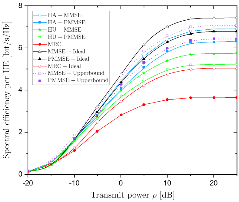
Figure 1: Uplink achievable SE per UE versus the power $\rho$ for SCF mMIMO systems with HA and HU MMSE and PMMSE decoding ($\sigma_{i}^{2}=1.58\cdot 10^{-4}$ for $i=\phi,\varphi$, $\kappa_{\mathrm{t}}=\kappa_{\mathrm{r}}=0.126$, and $\xi=1.6\sigma^{2}$).

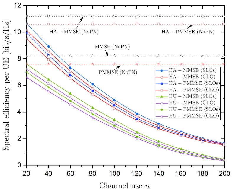
Figure 2: Uplink achievable SE per UE versus the channel use $n$ of the data transmission phase for SCF mMIMO systems with HA and HU MMSE and PMMSE decoding ($\sigma_{i}^{2}=1.58\cdot 10^{-4}$ for $i=\phi,\varphi$, $\kappa_{\mathrm{t}}=\kappa_{\mathrm{r}}=0$, and $\xi=1.6\sigma^{2}$).

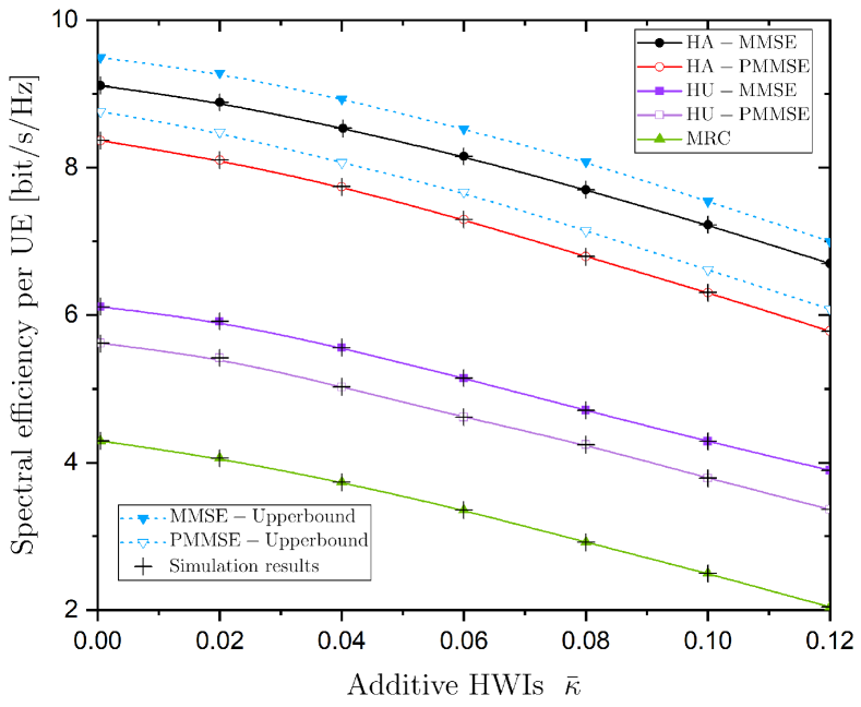
Figure 3: Uplink achievable SE per UE versus $\bar{\kappa}$ for SCF mMIMO systems with HA and HU MMSE and PMMSE decoding ($\sigma_{i}^{2}=0$ for $i=\phi,\varphi$, $\kappa_{\mathrm{t}}=\kappa_{\mathrm{r}}=0.126$, and $\xi=1.6\sigma^{2}$).

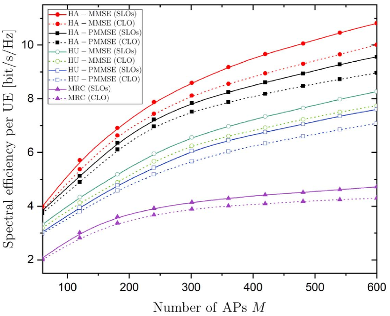
Figure 4: Uplink achievable SE per UE versus the number of APs $M$ for SCF mMIMO systems with HA and HU MMSE and PMMSE decoding ($\sigma_{i}^{2}=1.58\cdot 10^{-4}$ for $i=\phi,\varphi$, $\kappa_{\mathrm{t}}=\kappa_{\mathrm{r}}=0$, and $\xi=1.6\sigma^{2}$).

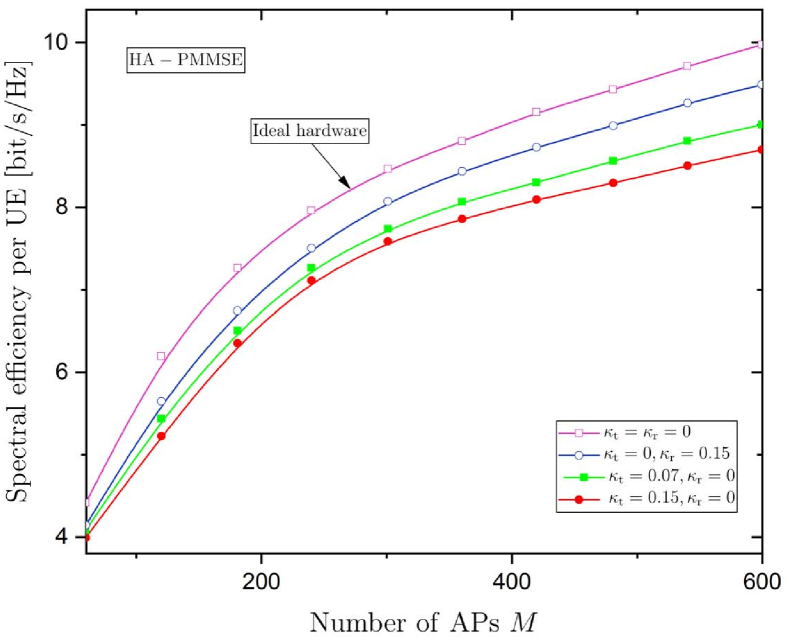
Figure 5: Uplink achievable SE per UE versus the number of APs $M$ for SCF mMIMO systems with HA and HU MMSE and PMMSE decoding ($\sigma_{i}^{2}=1.58\cdot 10^{-4}$ for $i=\phi,\varphi$, $\kappa_{\mathrm{t}}=\kappa_{\mathrm{r}}=0.126$, and $\xi=1.6\sigma^{2}$).

Keeping the additive HWIs equal to zero, Fig. 2 illustrates the variation of the achievable SE per user versus the channel use of the data transmission phase. In particular, in Fig. 2, the achievable SE decreases as the number of channel uses increases since the aggregate detrimental contribution from PN becomes higher. We also depict the SEs of MMSE and PMMSE receivers and their HA versions with no PN. These are constant with respect to $n$ since they do not depend on the PN being the only source of channel aging in this work. Next, in both HA-MMSE and HA-PMMSE receivers, the SLOs configuration outperforms the CLO design since the distortions from different LOs average out in the large system limit as described by [25, 16]. Moreover, the SEs for both HA-MMSE and HA-PMMSE receivers diminish with increasing $n$ since the phase drift becomes higher and the corresponding impact of PN becomes quite destructive. At the end of the data transmission, where $n=200$, the degradation is so heavy that the performance with scalable and conventional CF mMIMO systems becomes almost identical for both cases of HA and HU decoders.

Fig. 3 provides the performance of the achievable SE versus $\bar{\kappa}$, where $\kappa_{\mathrm{t}}=\bar{\kappa}$ and $\kappa{\mathrm{r}}=\bar{\kappa}+0.03$, while the effect of PN has not been considered to focus on the impact of the additive HWIs. The impact of PN is studied in other figures. The figure starts from the case of no additive HWIs at the BS when $\bar{\kappa}=0$ and ends with severe additive HWIs. Obviously, the higher the additive HWIs, the higher the degradation of the system performance becomes. Furthermore, it is evident that the practical SCF mMIMO systems perform very well since the proposed HA-PMMSE achieves just $9\%$ less SE with HA-MMSE receivers when $\bar{\kappa}=0.06$. When it comes to the HU decoders, the rates worsen with increasing the additive HWIs as well. Regarding the difference between the HA-PMMSE and PMMSE decoders is significant since it is approximately $2.6$ bit/s/Hz for all values of $\bar{\kappa}$. Also, we illustrate the superior performance of MMSE-style decoders against the MRC decoder as anticipated. Moreover, we provide the MMSE decoder given by Proposition 2. The provided tightness of the DE analytical expressions with respect to the simulation results, represented by the "cross" symbol, verifies Theorem 1.

Fig. 4 compares the SEs versus the number of APs $M$ in the HA and HU cases for both scalable and conventional CF mMIMO systems. We consider the impact of PN while the additive HWIs are not taken into account. In all cases, $\mathrm{\overline{SE}}_{k}^{\mathrm{lo}}$ increases with $M$. Moreover, we observe that SLOs achieve a better SE than the CLO design. Actually, the performance gap between the SLOs and CLO design increases with $M$ because the phase drifts are independent and in the large system limit, they are averaged, which is a benefit paid as a trade of a higher deployment cost [25, 35].

Fig. 5 depicts the impact of the additive HWIs on SCF mMIMO systems with a focus on the proposed HA-PMMSE combiner by showing the average achievable SE per UE versus the number of APs while the PN is assumed negligible. Obviously, the achievable SE increases $M$ but the additive HWIs at the APs side and UE sides behave differently. Of course, the presence of HWIs degrades the performance. Specifically, the additive HWIs at the transmit side, i.e., at the UE, have a more significant impact on the SE. For example, at $M=400$ APs, the loss due to the receive distortion is only $4\%$, while in the case of the transmit distortion, the degradation is $11\%$. Hence, the quality of hardware at the transmitter side should be considered more during the design.

VII Conclusion

In this paper, we investigated the impact of HWIs in SCF mMIMO systems, where the complexity at each AP is finite even when the number of UEs increases to infinity. Specifically, we introduced a general model with HWIs during the channel estimation, and we showed how HWIs modify the CSI. Moreover, we derived the HA-PMMSE combiner considering both HWIs and scalability design issues. Next, we obtained upper and lower bounds on the SE. In particular, we derived the DE of the achievable uplink SE, carrying the impact of HWIs, and we demonstrated the realistic performance of SCF mMIMO systems by varying the fundamental system parameters. This allowed us to extract insightful conclusions as guidelines for the practical implementation of these systems. Among the observations, we would like to highlight that the HA receivers outperform those which are hardware unaware of the presence of both additive HWIs and PN. Also, PMMSE should be preferred due to its advantages and because its performance loss is negligible compared to full MMSE not only in ideal scenarios but in realistic conditions where HWIs exist. Furthermore, we showed that even in SCF mMIMO systems, the HWIs result in ceilings at the SE, and that SCF mMIMO carries its benefits even under practical conditions. Future works should take into account the effect of limited capacity fronthaul links. Another interesting direction could be the extension of this work to full-duplex systems where self-interference arises as another hardware impairment [47].

Appendix A Proof of Proposition 2

We first assume that a genie is providing the received with perfect CSI and with the value of the multi-user interference term, which can then be subtracted from the received signal. What remains is a channel where the sum of the transmit and receive distortion, and noise is an independent circularly symmetric complex Gaussian distributed signal. As in [48], it follows that Gaussian signaling is optimal. An upper bound on the uplink capacity is

$$R_{k}=\frac{1}{\tau_{\mathrm{p}}}\!\!\sum_{n=1}^{\tau_{\mathrm{c}}-\tau_{\mathrm{p}}}\!\mathbb{E}\left\{\max_{{\mathbf{v}}_{k,n}:\|{\mathbf{v}}_{k,n}\|=1}\log_{2}\left(1+\gamma_{k,n}\left({\mathbf{v}}_{k,n}\right)\right)\right\}\!\!,$$ (48)

where we have obtained the upper bound for each $n$ in the transmission phase, and then, we have taken the average over these bounds [15]. The uplink SINR in (48) is

$$\!\!\gamma_{k,n}\!\left({\mathbf{v}}_{k,n}\right)\!=\!\frac{\rho_{k}{\mathbf{v}}_{k,n}^{{\scriptscriptstyle\mathsf{H}}}{\mathbf{D}}_{k}{{\mathbf{h}}}_{k,n}{{\mathbf{h}}}_{k,n}^{{\scriptscriptstyle\mathsf{H}}}{\mathbf{D}}_{k}{\mathbf{v}}_{k,n}}{{\mathbf{v}}_{k,n}^{{\scriptscriptstyle\mathsf{H}}}{\mathbf{D}}_{k}\tilde{{\mathbf{\Sigma}}}^{\dagger}{\mathbf{D}}_{k}{\mathbf{v}}_{k,n}},$$ (49)

where $\tilde{{\mathbf{\Sigma}}}$, ${\bm{\kappa}}_{\mathrm{r}}^{2}$ and ${\mathbf{F}}_{|{\mathbf{h}}_{i}|^{2}}$ are defined in Proposition 2. We have considered the pseudo-inverse of $\tilde{{\mathbf{\Sigma}}}$ instead of its inverse because the terms inside the parentheses may not be strictly positive definite [12].

The maximization of the achievable rate is obtained by noticing that the logarithm is a monotonically increasing function. Indeed, the optimization concerns a generalized Rayleigh quotient problem which is solved by (28) and achieves the upper bound given by (26) after plugging the maximizing combiner into (48).

Appendix B Proof of Lemma 2

The MSE definition between the estimated received signal, given by (25), and the transmit signal during the training phase $\left(n\in\{0,\tau\}\right)$ gives

$$\mathrm{MSE}_{k,n}=\mathbb{E}\left\{\|\hat{s}_{k,n}-{s}_{k,n}\|^{2}_{2}\big{|}\hat{{\mathbf{H}}}_{n}\right\}$$ (50)

$$=\tr\left(\mathbb{E}\left\{\left(\hat{s}_{k,n}-{s}_{k,n}\right)\left(\hat{s}_{k,n}-{s}_{k,n}\right)^{{\scriptscriptstyle\mathsf{H}}}\big{|}\hat{{\mathbf{H}}}_{n}\right\}\right)$$ (51)

$$=$$,

where we have considered that $\tr\!\left(\!\mathbb{E}\!\left\{\!{{\mathbf{h}}}_{i,n}{{\mathbf{h}}}_{i,n}^{{\scriptscriptstyle\mathsf{H}}}\big{|}\hat{{\mathbf{h}}}_{i,n}\!\right\}\!\right)\!=\!\tr\!\left(\!\hat{{\mathbf{h}}}_{i,n}\hat{{\mathbf{h}}}_{i,n}^{{\scriptscriptstyle\mathsf{H}}}\!+\!\tilde{{\mathbf{R}}}_{i}\!\right)$ with $\tilde{{\mathbf{R}}}_{i}\!=\!\mathbb{E}\!\left\{\!\tilde{{\mathbf{h}}}_{i,n}\tilde{{\mathbf{h}}}_{i,n}^{{\scriptscriptstyle\mathsf{H}}}|\hat{{\mathbf{h}}}_{i,n}\!\right\}$.

Appendix C Proof of Proposition 4

First, we follow the approach in [15] to compute the average achievable SE for each $n$ in the transmission phase, and then, we obtain the average over these SEs. The achievable SE per UE in (41) is obtained by taking into account the Gaussianity of the input symbols and by making a worst-case assumption regarding the computation of the mutual information [49, Theorem $1$], where the inter-user interference and the distortion noises are treated as independent Gaussian noise. Moreover, based on [40], the receiver treats the channel as deterministic with the gain $\mathbb{E}\{{\mathbf{v}}_{k,n}^{{\scriptscriptstyle\mathsf{H}}}{\mathbf{D}}_{k}{\bm{\Theta}}_{k,n}{{\mathbf{h}}}_{k}\}$ in the detection. In contrast, the deviation from the average effective channel gain is treated as worst-case Gaussian noise. Thus, we obtain $\tilde{\gamma}^{\mathrm{lo}}$, where the expectation operator in the various terms is taken concerning the channel vectors as well as the noise processes, which concludes the proof.

Appendix D Proof of Theorem 1

First, we obtain the DE of the desired signal power given by (42). Specifically, we have

$${\mathbf{v}}_{k,n}^{{\scriptscriptstyle\mathsf{H}}}{\mathbf{D}}_{k}{{\mathbf{h}}}_{k,n} =\hat{{\mathbf{h}}}_{k,n}^{{\scriptscriptstyle\mathsf{H}}}{\mathbf{D}}_{k}{{\mathbf{\Sigma}}}{\mathbf{D}}_{k}{{\mathbf{h}}}_{k,n}$$ (52)

$$=\frac{\frac{1}{W}\hat{{\mathbf{h}}}^{\scriptscriptstyle\mathsf{H}}_{k,n}{\mathbf{D}}_{k}{{\mathbf{\Sigma}}}_{k}{\mathbf{D}}_{k}\left(\hat{{\mathbf{h}}}_{k,n}+\tilde{{\mathbf{h}}}_{k,n}\right)}{1+\frac{q}{W}{\hat{{\mathbf{h}}}}^{\scriptscriptstyle\mathsf{H}}_{k,n}{\mathbf{D}}_{k}{{\mathbf{\Sigma}}}_{k}{\mathbf{D}}_{k}{\hat{{\mathbf{h}}}}_{k,n}}$$ (53)

$$\asymp\frac{\frac{1}{W}\hat{{\mathbf{h}}}^{\scriptscriptstyle\mathsf{H}}_{k,n}{\mathbf{D}}_{k}{{\mathbf{\Sigma}}}_{k}{\mathbf{D}}_{k}\hat{{\mathbf{h}}}_{k,n}}{1+\frac{q}{W}{\hat{{\mathbf{h}}}}^{\scriptscriptstyle\mathsf{H}}_{k,n}{\mathbf{D}}_{k}{{\mathbf{\Sigma}}}_{k}{\mathbf{D}}_{k}{\hat{{\mathbf{h}}}}_{k,n}},$$ (54)

where in (52), we have replaced the expression of the MMSE decoder given by (45). In the next equation, we have applied the matrix inversion lemma and used the orthogonality between the channel and its estimated version. Note that $q=\left(1+\kappa_{\mathrm{t}_{\mathrm{UE}}}^{2}\right)\rho_{k}$ while ${{\mathbf{\Sigma}}}_{k}^{\dagger}$ is defined as

$${{\mathbf{\Sigma}}}_{k}^{\dagger}\! =\!{{\mathbf{\Sigma}}}^{\dagger}-\frac{q}{W}{\mathbf{D}}_{k}\hat{{\mathbf{h}}}_{k,n}\hat{{\mathbf{h}}}_{k,n}^{{\scriptscriptstyle\mathsf{H}}}{\mathbf{D}}_{k}$$ (55)

$$\!=\!\displaystyle{\mathbf{D}}_{k}\!\!\left(\sum_{\begin{subarray}{c}i\in\mathcal{P}_{k}\\ i\neq k\end{subarray}}\!\!\frac{q}{W}\hat{{\mathbf{h}}}_{i,n}\hat{{\mathbf{h}}}_{i,n}^{{\scriptscriptstyle\mathsf{H}}}\!+\!\frac{{\bm{\kappa}}_{\mathrm{r}}^{2}}{W}\sum_{i\in\mathcal{P}_{k}}\!\rho_{i}{\mathbf{F}}_{|\hat{{\mathbf{h}}}_{i}|^{2}}\!+\!{\alpha\xi}{\bm{\mathrm{I}}}_{W}\!\!\right)\!\!{\mathbf{D}}_{k}\!+\!\tilde{{\bm{\Delta}}}.$$

In the numerator of (54), we have applied [50, Lem. B.26]. We continue with the use of [50, Lem. 14.3] known as rank-1 perturbation lemma, [50, Lem. B.26], and [51, Theorem 1] as

$${\mathbf{v}}_{k,n}^{{\scriptscriptstyle\mathsf{H}}}{\mathbf{D}}_{k}{\mathbf{h}}_{k,n} \asymp\frac{\frac{1}{W}\tr\left({\mathbf{D}}_{k}{\bm{\Phi}}_{k}{\mathbf{D}}_{k}{\mathbf{T}}\right)}{1+\frac{q}{W}\tr\left({\mathbf{D}}_{k}{\bm{\Phi}}_{k}{\mathbf{D}}_{k}{\mathbf{T}}\right)}$$ (56)

$$=\frac{\tilde{\delta}_{k}}{1+\delta_{k}},$$ (57)

where $\tilde{\delta}_{k}=\frac{1}{W}\tr{\mathbf{D}}_{k}{\bm{\Phi}}_{k}{\mathbf{D}}_{k}{\mathbf{T}}$ and $\delta_{k}=\frac{q}{W}\tr{\mathbf{D}}_{k}{\bm{\Phi}}_{k}{\mathbf{D}}_{k}{\mathbf{T}}$. The term, concerning the deviation from the average effective channel gain, becomes

$$\!\!\mathrm{Var}\left\{{\mathbf{v}}_{k,n}^{{\scriptscriptstyle\mathsf{H}}}{\mathbf{D}}_{k}{{\mathbf{h}}}_{k,n}\right\}\asymp\frac{\frac{1}{W}\mathbb{E}\left\{|\hat{{\mathbf{h}}}^{\scriptscriptstyle\mathsf{H}}_{k,n}{\mathbf{D}}_{k}{{\mathbf{\Sigma}}}_{k}{\mathbf{D}}_{k}{{\mathbf{h}}}_{k,n}|^{2}\right\}}{\left(1+\delta_{k}\right)^{2}}$$ (58)

$$~{}~{}~{}\asymp\frac{\mathbb{E}\left\{\frac{1}{W^{2}}\tr\left({\mathbf{D}}_{k}{\bm{\Phi}}_{k}{\mathbf{D}}_{k}{{\mathbf{\Sigma}}}_{k}{\mathbf{D}}_{k}\left({\mathbf{R}}_{k}-{\bm{\Phi}}_{k}\right){\mathbf{D}}_{k}{\mathbf{\Sigma}}_{k}\right)\right\}}{\left(1+\delta_{k}\right)^{2}}$$ (59)

$$~{}~{}~{}\asymp\frac{\mathbb{E}\left\{\frac{1}{W^{2}}\tr\left({\mathbf{D}}_{k}\left({\mathbf{R}}_{k}-{\bm{\Phi}}_{k}\right){\mathbf{D}}_{k}{\mathbf{T}}^{{}^{\prime}}_{k}\right)\right\}}{\left(1+\delta_{k}\right)^{2}},$$ (60)

where in (58), we have used the matrix inversion lemma, [50, Lem. B.26], and [51, Theorem 1]. In (59), we have applied the rank-1 perturbation lemma, [50, Lem. B.26], and [33, Lem. 10]. and [50, Lem. B.26] again. The last step includes application of [41, Theorem 2].
Based on (43), the interference power of the $k$th UE is written as

$$|{\mathbf{v}}_{k,n}^{{\scriptscriptstyle\mathsf{H}}}{\mathbf{D}}_{k}{{\mathbf{h}}}_{i,n}|^{2}\asymp\left|\frac{\frac{1}{W}\hat{{\mathbf{h}}}^{\scriptscriptstyle\mathsf{H}}_{k,n}{\mathbf{D}}_{k}{{\mathbf{\Sigma}}}_{k}{\mathbf{D}}_{k}{{\mathbf{h}}}_{i,n}}{1+\delta_{k}}\right|^{2}$$ (61)

$$\asymp\frac{\hat{{\mathbf{h}}}^{\scriptscriptstyle\mathsf{H}}_{k,n}{\mathbf{D}}_{k}{{\mathbf{\Sigma}}}_{k}{\mathbf{D}}_{k}{{\mathbf{h}}}_{i,n}{\mathbf{h}}_{i,n}^{{\scriptscriptstyle\mathsf{H}}}{\mathbf{D}}_{k}{{\mathbf{\Sigma}}}_{k}{\mathbf{D}}_{k}\hat{{\mathbf{h}}}_{k,n}}{W^{2}\left(1+\delta_{k}\right)^{2}}$$ (62)

$$\asymp\frac{{{\mathbf{h}}}^{\scriptscriptstyle\mathsf{H}}_{i,n}{\mathbf{D}}_{k}{{\mathbf{\Sigma}}}_{k}{\mathbf{D}}_{k}{\bm{\Phi}}_{k}{\mathbf{D}}_{k}{{\mathbf{\Sigma}}}_{k}{\mathbf{D}}_{k}{{\mathbf{h}}}_{i,n}}{W^{2}\left(1+\delta_{k}\right)^{2}}$$ (63)

$$\!\asymp\!\frac{1}{\left(1\!+\!\delta_{k}\right)^{2}}\bigg{(}\!\!\frac{1}{W^{2}}{{\mathbf{h}}}^{\scriptscriptstyle\mathsf{H}}_{i,n}{\mathbf{D}}_{k}{{\mathbf{\Sigma}}}_{ki}{\mathbf{D}}_{k}{\bm{\Phi}}_{k}{\mathbf{D}}_{k}{{\mathbf{\Sigma}}}_{ki}{\mathbf{D}}_{k}{{\mathbf{h}}}_{i,n}\!$$

$$+\!\frac{|{{\mathbf{h}}}^{\scriptscriptstyle\mathsf{H}}_{i,n}{\mathbf{D}}_{k}{{\mathbf{\Sigma}}}_{ki}{\mathbf{D}}_{k}\hat{{\mathbf{h}}}_{i,n}|^{2}\hat{{\mathbf{h}}}^{\scriptscriptstyle\mathsf{H}}_{i,n}{\mathbf{D}}_{k}{{\mathbf{\Sigma}}}_{ki}{\mathbf{D}}_{k}{\bm{\Phi}}_{k}{\mathbf{D}}_{k}{{\mathbf{\Sigma}}}_{ki}{\mathbf{D}}_{k}\hat{{\mathbf{h}}}_{i,n}}{W^{4}\left(1+\delta_{i}\right)^{2}}$$

$$-2\mathrm{Re}\bigg{\{}\frac{\left(\hat{{\mathbf{h}}}^{\scriptscriptstyle\mathsf{H}}_{i,n}{\mathbf{D}}_{k}{{\mathbf{\Sigma}}}_{ki}{\mathbf{D}}_{k}{{\mathbf{h}}}_{i,n}\right)}{W^{3}\left(1+\delta_{i}\right)^{2}}\left({{\mathbf{h}}}^{\scriptscriptstyle\mathsf{H}}_{i,n}{\mathbf{D}}_{k}{{\mathbf{\Sigma}}}_{ki}{\mathbf{D}}_{k}{\bm{\Phi}}_{k}{\mathbf{D}}_{k}{{\mathbf{\Sigma}}}_{ki}{\mathbf{D}}_{k}\hat{{\mathbf{h}}}_{i,n}\right)\!\!\!\bigg{\}}\!\bigg{)}$$ (64)

$$\asymp\frac{1}{\left(1+\delta_{k}\right)^{2}}\bigg{(}\zeta_{ki}+\frac{|\nu_{ki}|^{2}\mu_{ki}}{\left(1+\delta_{i}\right)^{2}}-2\mathrm{Re}\left\{\frac{\nu_{ki}^{*}\mu_{ki}}{\left(1+\delta_{i}\right)}\right\}\bigg{)},$$ (65)

where we have applied the matrix inversion lemma in (61), while in (62) and (63), we have used [50, Lem. B.26]. In (64), we have applied again the matrix inversion lemma, and in the last step, we have used the rank-1 perturbation lemma, [50, Lem. B.26], [51, Theorem 1], and [41, Theorem 2]. The definitions of the various parameters are given in the presentation of the theorem. Below, the terms, corresponding to the transmit and receive distortions, are derived. Specifically, we have

$$\sigma_{\mathrm{t}}^{2}=\sum_{i=1}^{K}\kappa_{\mathrm{t}}^{2}\rho_{i}\mathbb{E}\left\{|{\mathbf{v}}_{k,n}^{{\scriptscriptstyle\mathsf{H}}}{\mathbf{D}}_{k}{\mathbf{h}}_{i,n}|^{2}\right\}$$

$$=\kappa_{\mathrm{t}}^{2}\left(\rho_{k}\mathbb{E}\left\{|{\mathbf{v}}_{k,n}^{{\scriptscriptstyle\mathsf{H}}}{\mathbf{D}}_{k}{\mathbf{h}}_{k,n}|^{2}\right\}+\sum_{i\neq k}^{K}\rho_{i}\mathbb{E}\left\{|{\mathbf{v}}_{k,n}^{{\scriptscriptstyle\mathsf{H}}}{\mathbf{D}}_{k}{\mathbf{h}}_{i,n}|^{2}\right\}\right)$$

$$\asymp\!\frac{\kappa_{\mathrm{t}}^{2}}{\left(1\!+\!\delta_{k}\right)^{2}}\!\!\left(\!\rho_{k}{\tilde{\delta}^{2}_{k}}{}\!+\!\sum_{i\neq k}^{K}\!\rho_{i}\!\!\left(\!\zeta_{ki}\!+\!\frac{|\nu_{ki}|^{2}\mu_{ki}}{\left(1\!+\!\delta_{i}\right)^{2}}\!-\!2\mathrm{Re}\!\left\{\!\frac{\nu_{ki}^{*}\mu_{ki}}{\left(1\!+\!\delta_{i}\right)}\!\right\}\!\!\right)\!\!\right)\!\!,$$ (66)

where, in (66), we have substituted (57) and (65). Also, the deterministic $\sigma_{\mathrm{r}}^{2}$ as $W\to\infty$ becomes

$$\!\!\!\sigma_{\mathrm{r}}^{2}\! =\!\mathbb{E}\left\{{\mathbf{v}}_{k,n}^{{\scriptscriptstyle\mathsf{H}}}{\mathbf{D}}_{k}{\bm{\kappa}}_{\mathrm{r}}^{2}\!\left({\bm{\mathrm{I}}}_{W}\circ{\mathbf{H}}_{n}{\mathbf{P}}{\mathbf{H}}^{{\scriptscriptstyle\mathsf{H}}}_{n}\right){\mathbf{D}}_{k}{\mathbf{v}}_{k,n}\right\}$$ (67)

$$\!\!\!\asymp\!\frac{{\bm{\kappa}}_{\mathrm{r}}^{2}\mathbb{E}\left\{\tr\left({\mathbf{D}}_{k}\left({\bm{\mathrm{I}}}_{W}\circ{\mathbf{H}}_{n}{\mathbf{P}}{\mathbf{H}}^{{\scriptscriptstyle\mathsf{H}}}_{n}\right){\mathbf{D}}_{k}{\mathbf{\Sigma}}_{k}{\mathbf{D}}_{k}{\bm{\Phi}}_{k}{\mathbf{D}}_{k}{\mathbf{\Sigma}}_{k}\right)\right\}}{W^{2}\left(1+\delta_{k}\right)^{2}}$$

$$\!\!\!\asymp\!\frac{\eta_{k}^{{}^{\prime}}}{W^{2}\left(1+\delta_{k}\right)^{2}}\sum_{i=1}^{K}\rho_{i}\tr\left({\mathbf{D}}_{k}^{2}{\bm{\kappa}}_{\mathrm{r}}^{2}{\mathbf{R}}_{i}\right)\!,$$ (68)

where in (67) we have written the diagonal matrix in terms of a Hadamard product. Next, we have exploited the freeness between ${\mathbf{v}}_{k,n}{\mathbf{v}}_{k,n}^{{\scriptscriptstyle\mathsf{H}}}$ and the diagonal matrix ${\bm{\mathrm{I}}}_{W}\circ{\mathbf{H}}{\mathbf{H}}^{{\scriptscriptstyle\mathsf{H}}}$. Also, we have applied [50, Lem. B.26][51, Theorem 1], [41, Theorem 2], and [52, p. 207] while we have set $\eta^{{}^{\prime}}_{k}=\frac{1}{W}\tr{\mathbf{T}}^{{}^{\prime}}_{k}$. The DE of the last term of (43), corresponding to the ATN contribution, becomes

$$\|{\mathbf{v}}_{k,n}^{{\scriptscriptstyle\mathsf{H}}}{\mathbf{D}}_{k}\|^{2} \asymp\frac{\frac{1}{W^{2}}\hat{{\mathbf{h}}}_{k,n}^{{\scriptscriptstyle\mathsf{H}}}{\mathbf{D}}_{k}{\mathbf{\Sigma}}_{k}{\mathbf{D}}_{k}^{2}{\mathbf{\Sigma}}_{k}{\mathbf{D}}_{k}\hat{{\mathbf{h}}}_{k,n}}{\left(1+\delta_{k}\right)^{2}}$$ (69)

$$\asymp\frac{\frac{1}{W^{2}}\tr\left({\mathbf{\Sigma}}_{k}{\mathbf{D}}_{k}^{2}{\mathbf{\Sigma}}_{k}{\mathbf{D}}_{k}{\bm{\Phi}}_{k}{\mathbf{D}}_{k}\right)}{\left(1+\delta_{k}\right)^{2}}$$ (70)

$$=\frac{\frac{1}{W^{2}}\tr\left({\mathbf{T}}^{{}^{\prime\prime}}_{k}\right)}{\left(1+\delta_{k}\right)^{2}},$$ (71)

where in (69) and (70), we have applied the matrix inversion lemma and [50, Lem. B.26], respectively. In the last step, we have used the rank-1 perturbation lemma as well as [41, Theorem 2] and [51, Theorem 1]. By substituting (57), (60), (65), (66), (68), and (71) into (42) and (43), the DE SINR is derived and the proof is concluded.

solutionfile

References

- [1] A. K. Papazafeiropoulos et al., “Scalable cell-free massive MIMO systems with hardware impairments,” in IEEE 31st Annual International Symposium on Personal, Indoor and Mobile Radio Communications, May 2020, pp. 1–7.
- [2] T. Marzetta, “Noncooperative cellular wireless with unlimited numbers of base station antennas,” IEEE Trans. Wireless Commun., vol. 9, no. 11, pp. 3590–3600, Nov. 2010.
- [3] T. L. Marzetta et al., Fundamentals of Massive MIMO. Cambridge University Press, 2016.
- [4] E. Björnson, J. Hoydis, and L. Sanguinetti, “Massive MIMO networks: Spectral, energy, and hardware efficiency,” Foundations and Trends® in Signal Processing, vol. 11, no. 3-4, pp. 154–655, 2017.
- [5] H. Q. Ngo et al., “Cell-free massive MIMO versus small cells,” IEEE Trans. Wireless Commun., vol. 16, no. 3, pp. 1834–1850, Mar. 2017.
- [6] E. Björnson and L. Sanguinetti, “Making cell-free massive MIMO competitive with MMSE processing and centralized implementation,” IEEE Trans. Wireless Commun., vol. 19, no. 1, pp. 77–90, Jan. 2020.
- [7] A. Papazafeiropoulos et al., “Performance analysis of cell-free massive MIMO systems: A stochastic geometry approach,” IEEE Trans. Veh. Tech., vol. 69, no. 4, pp. 3523–3537, 2020.
- [8] A. K. Papazafeiropoulos et al., “Multipair two-way DF relaying with cell-free massive MIMO,” IEEE Open J. Commun. Soc., vol. 2, pp. 423–438, 2021.
- [9] A. Papazafeiropoulos et al., “Towards optimal energy efficiency in cell-free massive MIMO systems,” IEEE Trans. Green Commun. Net., vol. 5, no. 2, pp. 816–831, 2021.
- [10] S. Buzzi and C. D’Andrea, “Cell-free massive MIMO: User-centric approach,” IEEE Wireless Commun. Lett., vol. 6, no. 6, pp. 706–709, June 2017.
- [11] S. Buzzi et al., “User-centric 5G cellular networks: Resource allocation and comparison with the cell-free massive MIMO approach,” IEEE Trans. Wireless Commun., vol. 19, no. 2, pp. 1250–1264, Feb. 2020.
- [12] E. Björnson and L. Sanguinetti, “Scalable cell-free massive MIMO systems,” IEEE Tran. Commun., vol. 68, no. 7, pp. 4247–4261, July 2020.
- [13] E. Björnson et al., “Optimality properties, distributed strategies, and measurement-based evaluation of coordinated multicell OFDMA transmission,” IEEE Trans. Signal Process., vol. 59, no. 12, pp. 6086–6101, Dec. 2011.
- [14] J. Qi and S. Aïssa, “Analysis and compensation of I/Q imbalance in MIMO transmit-receive diversity systems,” IEEE Trans. Commun., vol. 58, no. 5, pp. 1546–1556, May 2010.
- [15] A. Pitarokoilis, S. Mohammed, and E. Larsson, “Uplink performance of time-reversal MRC in massive MIMO systems subject to phase noise,” IEEE Trans. Wireless Commun., vol. 14, no. 2, pp. 711–723, Feb. 2015.
- [16] A. K. Papazafeiropoulos, “Impact of general channel aging conditions on the downlink performance of massive MIMO,” IEEE Trans. Veh. Tech., vol. 66, no. 2, pp. 1428–1442, Feb. 2017.
- [17] J. Qi and S. Aïssa, “On the power amplifier nonlinearity in MIMO transmit beamforming systems,” IEEE Trans. Commun., vol. 60, no. 3, pp. 876–887, Mar. 2012.
- [18] T. Schenk, RF imperfections in high-rate wireless systems: impact and digital compensation. Springer Science & Business Media, 2008.
- [19] C. Studer, M. Wenk, and A. Burg, “MIMO transmission with residual transmit-RF impairments,” in ITG/IEEE Work. Smart Ant. (WSA). IEEE, 2010, pp. 189–196.
- [20] J. Zhang et al., “Performance analysis and power control of cell-free massive MIMO systems with hardware impairments,” IEEE Access, vol. 6, pp. 55 302–55 314, June 2018.
- [21] X. Zhang et al., “Secure communications over cell-free massive MIMO networks with hardware impairments,” IEEE Syst. J., vol. 14, no. 2, pp. 1909–1920, Feb. 2020.
- [22] H. Masoumi and M. J. Emadi, “Performance analysis of cell-free massive MIMO system with limited fronthaul capacity and hardware impairments,” IEEE Trans. Wireless Commun., vol. 19, no. 2, pp. 1038–1053, Feb. 2020.
- [23] X. Hu et al., “Cell-free massive MIMO systems with low resolution ADCs,” IEEE Trans. Commun., vol. 67, no. 10, pp. 6844–6857, Oct. 2019.
- [24] J. Zheng et al., “Efficient receiver design for uplink cell-free massive MIMO with hardware impairments,” IEEE Trans. Veh. Tech., vol. 69, no. 4, pp. 4537–4541, Apr. 2020.
- [25] E. Björnson, M. Matthaiou, and M. Debbah, “Massive MIMO with non-ideal arbitrary arrays: Hardware scaling laws and circuit-aware design,” IEEE Trans. Wireless Commun., vol. 14, no. 8, pp. 4353–4368, Aug. 2015.
- [26] S. Perlman and A. Forenza, “An introduction to pcell,” Artemis Networks white paper, 2015.
- [27] G. Interdonato et al., “Ubiquitous cell-free massive MIMO communications,” EURASIP J. Wireless Commun. Net., vol. 2019, no. 1, p. 197, Jan. 2019.
- [28] D. Neumann, M. Joham, and W. Utschick, “Covariance matrix estimation in massive MIMO,” IEEE Signal Process. Lett., vol. 25, no. 6, pp. 863–867, June 2018.
- [29] K. Upadhya and S. A. Vorobyov, “Covariance matrix estimation for massive MIMO,” IEEE Signal Process. Lett., vol. 25, no. 4, pp. 546–550, Apr. 2018.
- [30] Ö. T. Demir et al., “Foundations of user-centric cell-free massive MIMO,” Foundations and Trends® in Signal Processing, vol. 14, no. 3-4, pp. 162–472.
- [31] J. Joung et al., “A survey on power-amplifier-centric techniques for spectrum-and energy-efficient wireless communications,” IEEE Commun. Surveys & Tut., vol. 17, no. 1, pp. 315–333, Jan. 2014.
- [32] D. Petrovic, W. Rave, and G. Fettweis, “Effects of phase noise on OFDM systems with and without PLL: Characterization and compensation,” IEEE Trans. Commun., vol. 55, no. 8, pp. 1607–1616, Aug. 2007.
- [33] R. Krishnan et al., “Linear massive MIMO precoders in the presence of phase noise-A large-scale analysis,” IEEE Trans. Veh. Tech., vol. 65, no. 5, pp. 3057–3071, May 2016.
- [34] H. Holma and A. Toskala, LTE for UMTS: Evolution to LTE-Advanced, Wiley, Ed., 2011.
- [35] A. Papazafeiropoulos, B. Clerckx, and T. Ratnarajah, “Rate-splitting to mitigate residual transceiver hardware impairments in massive MIMO systems,” IEEE Trans. Veh. Tech., vol. 66, no. 9, pp. 8196–8211, Sep. 2017.
- [36] E. Björnson, E. G. Larsson, and T. L. Marzetta, “Massive MIMO: Ten myths and one critical question,” IEEE Commun. Mag., vol. 54, no. 2, pp. 114–123, Feb. 2016.
- [37] E. Björnson et al., “Massive MIMO systems with non-ideal hardware: Energy efficiency, estimation, and capacity limits,” IEEE Trans. Inf. Theory, vol. 60, no. 11, pp. 7112–7139, Nov. 2014.
- [38] S. Zarei et al., “Multi-cell massive MIMO systems with hardware impairments: Uplink-downlink duality and downlink precoding,” IEEE Trans. Wireless Commun., vol. 16, no. 8, pp. 5115–5130, Aug. 2017.
- [39] E. Nayebi et al., “Precoding and power optimization in cell-free massive MIMO systems,” IEEE Trans. Wireless Commun., vol. 16, no. 7, pp. 4445–4459, July 2017.
- [40] M. Medard, “The effect upon channel capacity in wireless communications of perfect and imperfect knowledge of the channel,” IEEE Trans. Inf. Theory, vol. 46, no. 3, pp. 933–946, May 2000.
- [41] J. Hoydis, S. ten Brink, and M. Debbah, “Massive MIMO in the UL/DL of cellular networks: How many antennas do we need?” IEEE J. Select. Areas Commun., vol. 31, no. 2, pp. 160–171, Feb. 2013.
- [42] R. Couillet and M. Debbah, Random matrix methods for wireless communications. Cambridge University Press, 2011.
- [43] A. K. Papazafeiropoulos and T. Ratnarajah, “Deterministic equivalent performance analysis of time-varying massive MIMO systems,” IEEE Trans. Wireless Commun., vol. 14, no. 10, pp. 5795–5809, Oct. 2015.
- [44] 3GPP, “Further advancements for E-UTRA physical layer aspects (Release 9),” 3GPP TS 36.814, Tech. Rep., 2017.
- [45] A. Papazafeiropoulos and T. Ratnarajah, “Towards a realistic assessment of multiple antenna HCNs: Residual additive transceiver hardware impairments and channel aging,” IEEE Trans. Veh. Tech., vol. 66, no. 10, pp. 9061–9073, Oct. 2017.
- [46] A. Papazafeiropoulos et al., “Nuts and bolts of a realistic stochastic geometric analysis of mmWave HetNets: Hardware impairments and channel aging,” IEEE Trans. Veh. Tech., vol. 68, no. 6, pp. 5657–5671, June 2019.
- [47] Y. Zhang et al., “Power scaling of full-duplex two-way millimeter-wave relay with massive MIMO,” IEEE Trans. Veh. Tech., vol. 69, no. 12, pp. 15 298–15 313, 2020.
- [48] E. Telatar, “Capacity of multi-antenna gaussian channels,” Europ. Trans. on Telecom., vol. 10, no. 6, pp. 585–595, June 1999.
- [49] B. Hassibi and B. Hochwald, “How much training is needed in multiple-antenna wireless links?” IEEE Trans. Inform. Theory, vol. 49, no. 4, pp. 951–963, Apr. 2003.
- [50] Z. Bai and J. W. Silverstein, Spectral analysis of large dimensional random matrices. Springer, 2010, vol. 20.
- [51] S. Wagner et al., “Large system analysis of linear precoding in correlated MISO broadcast channels under limited feedback,” IEEE Trans. Inform. Theory, vol. 58, no. 7, pp. 4509–4537, July 2012.
- [52] T. Tao, Topics in random matrix theory. American Mathematical Soc., 2012, vol. 132.