Testing the Planar Straight-line Realizability of 2-Trees
with Prescribed Edge Lengths

Abstract

We study a classic problem introduced thirty years ago by Eades and Wormald. Let $G=(V,E,\lambda)$ be a weighted planar graph, where $\lambda:E\rightarrow\mathbb{R}^{+}$ is a length function. The Fixed Edge-Length Planar Realization problem (FEPR for short) asks whether there exists a planar straight-line realization of $G$, i.e., a planar straight-line drawing of $G$ where the Euclidean length of each edge $e\in E$ is $\lambda(e)$.

Cabello, Demaine, and Rote showed that the FEPR problem is -hard, even when $\lambda$ assigns the same value to all the edges and the graph is triconnected. Since the existence of large triconnected minors is crucial to the known -hardness proofs, in this paper we investigate the computational complexity of the FEPR problem for weighted $2$-trees, which are $K_{4}$-minor free. We show the -hardness of the problem, even when $\lambda$ assigns to the edges only up to four distinct lengths. Conversely, we show that the FEPR problem is linear-time solvable when $\lambda$ assigns to the edges up to two distinct lengths, or when the input has a prescribed embedding. Furthermore, we consider the FEPR problem for weighted maximal outerplanar graphs and prove it to be linear-time solvable if their dual tree is a path, and cubic-time solvable if their dual tree is a caterpillar. Finally, we prove that the FEPR problem for weighted $2$-trees is slice-wise polynomial in the length of the longest path.

1 Introduction

The problem of producing drawings of graphs with geometric constraints is a core subject in Graph Drawing (see, e.g., [3, 4, 5, 12, 16, 25, 26, 29, 36, 42, 46, 48]). In this context, a classic question is the one of testing whether a graph can be drawn planarly so that its edges are straight-line segments of prescribed lengths. The study of such a question has connections with several topics in computational geometry [19, 44, 51], rigidity theory [18, 32, 34], structural analysis of molecules [9, 33], and sensor networks [15, 40, 43]. Formally, given a weighted planar graph $G=(V,E,\lambda)$, i.e., a planar graph with vertex set $V$ and edge set $E$ equipped with a length function $\lambda:E\rightarrow\mathbb{R}^{+}$, the Fixed Edge-Length Planar Realization problem (FEPR, for short) asks whether there exists a planar straight-line realization of $G$, i.e., a planar straight-line drawing of $G$ in the plane where the Euclidean length of each edge $e\in E$ is $\lambda(e)$. The FEPR problem was first studied by Eades and Wormald [28], who showed its -hardness even for triconnected planar graphs and for biconnected planar graphs with unit lengths. Cabello, Demaine, and Rote strengthened this result by proving -hardness even for triconnected planar graphs with unit lengths [14]. The graphs that admit a planar straight-line realization with unit lengths are also called matchstick graphs. Abel et al. [1] showed that recognizing matchstick graphs is strongly $\exists\mathbb{R}$-complete, solving an open problem stated by Schaefer [45].

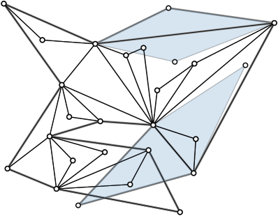
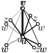
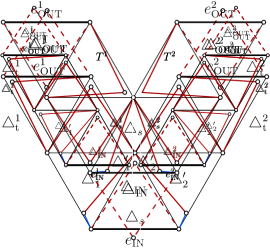
Since the existence of large triconnected minors is essential in the known hardness proofs of the FEPR problem, we study its computational complexity for weighted $2$-trees, which are the maximal graphs with no K₄-minor. A $2$-tree is a graph composed of $3$-cycles glued together along edges in a tree-like fashion. As an example, Fig. 1 shows a planar and a non-planar straight-line realization of the same weighted $2$-tree. The class of $2$-trees has been deeply studied in Graph Drawing (e.g., in [20, 27, 30, 35, 41]); such a graph class coincides with the one of the maximal series-parallel graphs. In particular, the edge lengths of planar straight-line drawings of $2$-trees have been studied in [10, 11].

First, we show that, in the fixed embedding setting, the FEPR problem can be solved in linear time (Section 3). We remark that the FEPR problem is -hard for general weighted planar graphs with fixed embedding [14, 28]. Second, we show that, in the variable embedding setting, the FEPR problem is -hard when the number of distinct lengths is at least four (Section 4), whereas it is linear-time solvable when the number of distinct lengths is $1$ or $2$ (Section 5). Note that, for general weighted planar graphs, the problem is -hard even when all the edges are required to have the same length [28]. Third, we move our attention to maximal outerplanar graphs (Section 6), which form a notable subclass of $2$-trees. We show that the FEPR problem can be solved in linear time for maximal outerpaths, i.e., the maximal outerplanar graphs whose dual tree is a path, and in cubic time for maximal outerpillars, i.e., the maximal outerplanar graphs whose dual tree is a caterpillar. Finally, we present a slice-wise polynomial algorithm for weighted $2$-trees, parameterized by the length of the longest path (Section 7). Section 2 contains preliminaries and Section 8 provides conclusions and open problems.

Similarly to [14], in our algorithms, we adopt the real RAM model of computation, which is customary in computational geometry and allows us to perform standard arithmetic operations in constant time. Furthermore, we show NP-hardness in the Turing machine model by exploiting lengths whose encoding has constant size.

Figure 1: A planar and a non-planar straight-line realization of the same weighted $2$-tree.

2 Preliminaries

Throughout the paper, we assume that graphs are connected and simple (i.e., with no loops or parallel edges). Moreover, whenever we refer to the length of a segment or to the distance of two geometric objects, we always assume that these are measured according to the Euclidean metric.

Drawings and embeddings.

A drawing $\Gamma$ of a graph is a mapping of each vertex $v$ to a distinct point $\Gamma(v)$ in the plane and of each edge $(u,v)$ to a Jordan arc $\Gamma(u,v)$ with endpoints $\Gamma(u)$ and $\Gamma(v)$. We often use the same notation for a vertex $v$ and the point $\Gamma(v)$. A drawing is planar if it contains no two crossing edges and it is straight-line if each curve representing an edge is a straight-line segment. A planar drawing partitions the plane into connected regions, called faces. The bounded faces are the internal faces, while the unbounded face is the outer face. The boundary of a face is the circular list of vertices and edges encountered when traversing the geometric border of the face. A graph $G$ is planar if it admits a planar drawing. A planar drawing of $G$ defines a clockwise order of the edges incident to each vertex of $G$; the set of such orders for all the vertices is a rotation system for $G$. Two planar drawings of $G$ are equivalent if (i) they define the same rotation system for $G$ and (ii) their outer faces have the same boundaries. An equivalence class of planar drawings is a plane embedding (or simply an embedding). When referring to a planar drawing $\Gamma$ of a graph that has a prescribed embedding $\mathcal{E}$, we always imply that $\Gamma$ is in the equivalence class $\mathcal{E}$; when we want to stress this fact, we say that $\Gamma$ respects $\mathcal{E}$. All the planar drawings respecting the same embedding have the same set of face boundaries. Hence, we can talk about the face boundaries of a graph with a prescribed embedding. With a little overload of terminology, we sometimes write face of a graph with a prescribed embedding, while referring to the boundary of the face. A graph is biconnected if the removal of any vertex leaves the graph connected. In any planar drawing of a biconnected graph every face is bounded by a simple cycle. Let $\Gamma$ be a drawing of a graph $G$ and let $G^{\prime}$ be a subgraph of $G$; the restriction of $\Gamma$ to $G^{\prime}$ is the drawing of $G^{\prime}$ obtained by removing from $\Gamma$ the vertices and edges of $G$ that are not in $G^{\prime}$.

2-trees and maximal outerplanar graphs.

A $2$-tree is recursively defined as follows. A cycle formed by $k$ edges is a $k$-cycle. A $3$-cycle is a $2$-tree. Given a $2$-tree $G$ containing the edge $(u,w)$, the graph obtained by adding to $G$ a vertex $v$ and two edges $(v,u)$ and $(v,w)$ is a $2$-tree. We observe that any $2$-tree $G$ satisfies the following properties:

1. $G$ is biconnected;

2. the two neighbors of any degree-$2$ vertex of $G$ are adjacent; and

3. if $|V(G)|\geq 4$, then $G$ contains two non-adjacent degree-$2$ vertices.

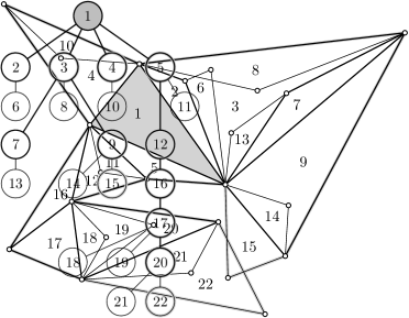
A $2$-tree $G$ is essentially composed of $3$-cycles glued together along edges in a tree-like fashion. We encode this tree-like structure in a tree we call the decomposition tree of $G$. This tree has a node for each $3$-cycle of $G$, and an edge between two nodes if the corresponding $3$-cycles have a common edge; see Fig. 2. Let $T$ be the decomposition tree of $G$, and $n$ be the number of nodes of $G$. We observe that $T$ is unique and contains $n-2$ nodes. Typically, $T$ is rooted at a $3$-cycle $c$ of $G$. We can compute $T$ rooted at $c$ by a recursive construction in which, together with $T$, we produce an auxiliary labeling of the edges of $G$. An edge $e$ is labeled with the highest node in $T$ whose corresponding $3$-cycle contains $e$. The construction is as follows. If $G$ coincides with $c$, then $T$ is a unique root node representing $c$, and each edge of $c$ is labeled with $c$ itself. Otherwise, by Property (P3), there is at least one degree-two vertex not belonging to $c$. Let $v$ be any such a vertex, let $u$ and $w$ be the vertices adjacent to $v$, and let $c^{*}$ be the $3$-cycle with vertices $u$, $v$, and $w$. Let $T^{*}$ denote the decomposition tree of $G-v$ rooted at $c$. We obtain $T$ by adding to $T^{*}$ a leaf representing $c^{*}$, whose parent is the node corresponding to the label of the edge $(u,w)$. Further, we set to $c^{*}$ the labels of the edges $(v,u)$ and $(v,w)$. It is not hard to see that this procedure constructs $T$ in $O(n)$ time.

Figure 2: On the left, a $2$-tree $G$. On the right, the decomposition tree of $G$ rooted at $\triangle_{1}$. Internal nodes are drawn with thick lines and leaf nodes of are drawn with thin lines.

An outerplanar drawing is a planar drawing in which all the vertices are incident to the outer face. A graph is outerplanar if it admits an outerplanar drawing. An outerplane embedding is an equivalence class of outerplanar drawings of a graph; note that a biconnected outerplanar graph has a unique outerplane embedding [39, 47]. An outerplanar graph is maximal if no edge can be added to it without losing outerplanarity. In the unique outerplane embedding of a maximal outerplanar graph, every internal face is delimited by a $3$-cycle. The dual tree $T$ of a biconnected outerplanar graph $G$ is defined as follows. Consider the (unique) outerplane embedding $\mathcal{O}$ of $G$. Then $T$ has a node for each internal face of $\mathcal{O}$ and has an edge between two nodes if the corresponding faces of $\mathcal{O}$ are incident to the same edge of $G$. An outerpath is a biconnected outerplanar graph whose dual tree is a path. A caterpillar is a tree that becomes a path if its leaves are removed. Such path is called the spine of the caterpillar. An outerpillar is a biconnected outerplanar graph whose dual tree is a caterpillar.

Straight-line realizations.

A weighted graph $G=(V,E,\lambda)$ is a graph equipped with a length function $\lambda$ that assigns a positive real number to each edge. A straight-line realization of $G$ is a straight-line drawing of $G$ in which each edge $e$ is drawn as a line segment of length $\lambda(e)$. If the drawing is planar, we say that the realization is planar. The Fixed Edge-Length Planar Realization (FEPR) problem receives as input a weighted planar graph $G$, and asks if there exists a planar straight-line realization of $G$.

In a straight-line realization of $G$, each $3$-cycle is realized as a triangle. Hence, if the lengths of the edges of at least one $3$-cycle do not respect the triangle inequality, then $G$ does not admit any (even non-planar) straight-line realization. We can trivially test in $O(n)$ time whether the length function of an $n$-vertex weighted $2$-tree is such that every $3$-cycle satisfies the triangle inequality. Hereafter we assume that every weighted $2$-tree satisfies this necessary condition.

In our proofs and algorithms, when clear from the context, we refer interchangeably to the $3$-cycles of a $2$-tree $G$, the nodes of its decomposition tree, and the triangles in a straight-line realization of $G$.

Triangles in a planar straight-line realization.

Let $G=(V,E,\lambda)$ be a weighted $2$-tree and $\Gamma$ be a planar straight-line realization of $G$. We denote with $\triangle_{i}$ a triangle drawn in $\Gamma$, that is, the straight-line realization of a $3$-cycle of $G$. Consider two triangles $\triangle_{i}$ and $\triangle_{j}$. We say that $\triangle_{i}$ is drawn inside $\triangle_{j}$ if all the points of $\triangle_{i}$ are points of $\triangle_{j}$ and at least one vertex of $\triangle_{i}$ is an interior point of $\triangle_{j}$. In the planar straight-line realization shown in Fig. 2, the triangles $\triangle_{6}$, $\triangle_{7}$, and $\triangle_{8}$ are drawn inside the triangle $\triangle_{3}$. Observe that, if $\triangle_{i}$ is drawn inside $\triangle_{j}$, then $\triangle_{i}$ and $\triangle_{j}$ have at most two common vertices. On the other hand, in general, $\triangle_{i}$ can be drawn inside $\triangle_{j}$ regardless of their distance in the decomposition tree of $G$. We have the following observation, which we use implicitly (and sometimes explicitly) in the paper.

Observation 2.1.

Let $\ell_{i}$ and $\ell_{j}$ be the lengths of the longest sides of two triangles $\triangle_{i}$ and $\triangle_{j}$, respectively. If $\ell_{i}>\ell_{j}$, then $\triangle_{i}$ is not drawn in $\triangle_{j}$. If $\ell_{i}=\ell_{j}$ and $\triangle_{i}$ is drawn inside $\triangle_{j}$, then $\triangle_{i}$ and $\triangle_{j}$ share a side of length $\ell_{i}=\ell_{j}$.

Of special interest for us is the case in which $\triangle_{i}$ and $\triangle_{j}$ share an edge. If such case occurs, then $\triangle_{i}$ and $\triangle_{j}$ are either adjacent or siblings in the decomposition tree of $G$. We have the following.

Observation 2.2.

Let $\triangle_{i}$ and $\triangle_{j}$ be two triangles sharing an edge with end-vertices $a$ and $b$. Let $\alpha_{i}$ and $\beta_{i}$ ($\alpha_{j}$ and $\beta_{j}$) denote the interior angles of $\triangle_{i}$ (resp., $\triangle_{j}$) at $a$ and $b$, respectively. If $\triangle_{i}$ is drawn inside $\triangle_{j}$, then $\alpha_{i}<\alpha_{j}$ and $\beta_{i}<\beta_{j}$.

We derive further useful properties by considering specific types of triangles. Consider an isosceles triangle with base of length $b$ and two sides of length $l$. We say the triangle is tall isosceles if $l>b$, and flat isosceles if instead $l<b$.

Lemma 1.

Let $\triangle_{i}$ and $\triangle_{j}$ be two triangles sharing an edge.

1. If $\triangle_{i}$ is tall isosceles and $\triangle_{j}$ is flat isosceles, then $\triangle_{i}$ is not drawn inside $\triangle_{j}$.

2. If $\triangle_{i}$ is tall isosceles and $\triangle_{j}$ is equilateral, then $\triangle_{i}$ is not drawn inside $\triangle_{j}$.

3. If $\triangle_{i}$ is equilateral and $\triangle_{j}$ is flat isosceles, then $\triangle_{i}$ is not drawn inside $\triangle_{j}$.

Proof.

All the statements follow from Theorem 2.2 and the facts that (i) a tall isosceles triangle has one interior angle smaller than $60^{\circ}$ and two interior angles greater than $60^{\circ}$, and (ii) a flat isosceles triangle has one interior angle greater than $60^{\circ}$ and two interior angles smaller than $60^{\circ}$. Refer to Fig. 3. ∎

(a)

(b)

(c)

Figure 3: Illustration for Lemma 1. The angles in gray are smaller than $60^{\circ}$ and the angles in white are greater than $60^{\circ}$. (3(a)) A tall isosceles triangle ($\triangle_{2}$, $\triangle_{3}$, $\triangle_{4}$, and $\triangle_{4}$) is not drawn inside a flat isosceles triangle ($\triangle_{1}$), (3(b)) A tall isosceles triangle ($\triangle_{2}$ and $\triangle_{3}$) is not drawn inside an equilateral triangle ($\triangle_{1}$), and (3(c)) An equilateral triangle ($\triangle_{2}$ and $\triangle_{3}$) is not drawn inside a flat isosceles triangle ($\triangle_{1}$).

Consider now three triangles $\triangle_{i}$, $\triangle_{j}$, $\triangle_{k}$ such that $\triangle_{j}$ and $\triangle_{k}$ share a side with $\triangle_{i}$. If the three triangles have a common side, then a necessary condition for $\triangle_{i}$ and $\triangle_{j}$ to be drawn inside $\triangle_{i}$ is given by Theorem 2.2. If instead there is no common side between $\triangle_{j}$ and $\triangle_{k}$, then we have the following lemmas.

Lemma 2.

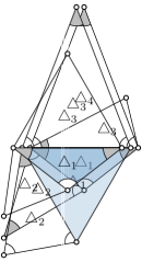
Let $\ell_{1}$ and $\ell_{2}$ be two lengths such that $2\ell_{2}>\ell_{1}>\ell_{2}$, and $\triangle_{i}$, $\triangle_{j}$, $\triangle_{k}$ be three triangles such that:

• $\triangle_{i}$ is an equilateral triangle with sides of length $\ell_{1}$,

• $\triangle_{j}$ and $\triangle_{k}$ are congruent flat isosceles triangles with base of length $\ell_{1}$ and two sides of length $\ell_{2}$,

• $\triangle_{i}$ shares one side with $\triangle_{j}$ and another side with $\triangle_{k}$, and

• $\triangle_{j}$ and $\triangle_{k}$ are drawn inside $\triangle_{i}$ and do not overlap with each other.

Then $\frac{\ell_{1}}{\ell_{2}}>\sqrt{3}\simeq 1.73$.

Proof.

Refer to Fig. 4. Let $v$ be the common vertex between $\triangle_{i}$, $\triangle_{j}$, and $\triangle_{k}$. Since $\triangle_{i}$ is equilateral the interior angle of $\triangle_{i}$ at $v$ is $60^{\circ}$. Hence, since $\triangle_{j}$ and $\triangle_{k}$ are congruent and intersect only at $v$ (they do not overlap), the internal angle $\alpha$ of both $\triangle_{j}$ and $\triangle_{k}$ at $v$ is at most $30^{\circ}$. We thus have that $\ell_{1}=2\ell_{2}\cos(\alpha)>2\ell_{2}\cos(30^{\circ})=\sqrt{3}{\ell_{2}}$. ∎

Figure 4: Illustration for Lemma 2: If two flat isosceles triangles ($\triangle_{j}$ and $\triangle_{k}$) are drawn inside an equilateral triangle ($\triangle_{i}$), then $\frac{\ell_{1}}{\ell_{2}}>\sqrt{3}$. The black point is the circumcenter of $\triangle_{i}$.

3 Prescribed Embedding

In this section, we describe an $O(n)$-time algorithm to solve the FEPR problem for an $n$-vertex $2$-tree whose embedding or whose rotation system is prescribed.

We start by showing how to check in linear time whether a straight-line realization of a $2$-tree with prescribed embedding is a planar straight-line realization respecting the embedding. This basic tool will be exploited throughout the paper.

Theorem 3.1.

Let $G=(V,E,\lambda)$ be an $n$-vertex weighted $2$-tree, $\mathcal{E}$ be a plane embedding of $G$, and $\Gamma$ be a straight-line realization of $G$. There exists an $O(n)$-time algorithm that tests whether $\Gamma$ is a planar straight-line realization respecting $\mathcal{E}$.

Proof.

First, we check whether $\Gamma$ respects $\mathcal{E}$. This can be done in $O(n)$ time by checking: (i) whether the clockwise order of the edges incident to each vertex in $\Gamma$ is the same as in $\mathcal{E}$; and (ii) whether the cycle bounding the outer face of $\Gamma$ (if $\Gamma$ is planar) is the same as in $\mathcal{E}$. More in detail, this check is as follows.

• Check (i) only requires to scan, for each vertex $v$ of $G$, the list representing the clockwise order of the edges incident to $v$ in $\mathcal{E}$, and to confirm that the slopes of such edges in $\Gamma$ form a decreasing sequence (where the slope of one of such edges is the one of the half-ray from $v$ through the other end-vertex of the edge and has a value between the slope $s$ of the first considered edge and $s-360^{\circ}$). This can be done in time proportional to the degree of $v$ and hence in $O(n)$ time over all the vertices of $G$.

• In order to perform check (ii), we find in $O(n)$ time the vertices $v_{\leftarrow}$ and $v_{\rightarrow}$ with smallest and largest $x$-coordinates, respectively, among the vertices of the cycle $\mathcal{C}$ bounding the outer face of $\mathcal{E}$. Then we check whether the edge that leaves $v_{\leftarrow}$ in clockwise direction along $\mathcal{C}$ lies above the edge that enters $v_{\leftarrow}$ in clockwise direction along $\mathcal{C}$ in $\Gamma$. Together with check (i), this guarantees that all the edges incident to vertices of $\mathcal{C}$ leave the vertices in $\mathcal{C}$ towards the region inside $\mathcal{C}$ in $\Gamma$, if $\Gamma$ is planar. It might still be the case, however, that $\mathcal{C}$ self-intersects or that other edges of $G$ cross $\mathcal{C}$, hence at this point we can guarantee that $\mathcal{C}$ bounds the outer face of $\Gamma$ only by assuming its planarity.

In order to check whether $\Gamma$ is planar, we augment $\Gamma$ to a straight-line drawing $\Gamma^{\prime}$ of a maximal planar graph so that, if $\Gamma$ is planar, then $\Gamma^{\prime}$ is planar, as well. This is done as follows. If $\Gamma$ is a planar straight-line realization respecting $\mathcal{E}$, every internal face $f$ of $\mathcal{E}$ is bounded in $\Gamma$ by a polygon $\mathcal{P}_{f}$ whose interior is empty. We triangulate the interior of $\mathcal{P}_{f}$ by the addition of dummy edges. This can be done in linear time over all the internal faces of $\mathcal{E}$ by means of the algorithm by Chazelle [17]. We also triangulate the outer face of $\Gamma$. This is done similarly as described by Cabello et al. [14]. Namely, we enclose $\Gamma$ into a large equilateral triangle $T$ with a horizontal side $\ell$. This partitions the outer face of $\Gamma$ into two regions, namely a bounded region $\mathcal{R}$ and an unbounded region $\mathcal{R}^{\prime}$. We then add edges from $v_{\leftarrow}$ and $v_{\rightarrow}$ to the left and right end-vertices of $\ell$, respectively. This subdivides $\mathcal{R}$ into two regions delimited by simple polygons. We triangulate the interior of such polygons, again using Chazelle’s algorithm [17]. Denote by $\Gamma^{\prime}$ the resulting straight-line drawing.

If $\Gamma$ is a planar straight-line realization respecting $\mathcal{E}$, then (as described in [14]) every execution of Chazelle’s algorithm terminates correctly. Hence, if at least one of the executions of Chazelle’s algorithm terminates in error, we conclude that $\Gamma$ is not a planar straight-line realization respecting $\mathcal{E}$. It might also be the case that every execution of Chazelle’s algorithm terminates correctly and yet $\Gamma$ contained crossings. Hence, we also need to check whether $\Gamma^{\prime}$ is planar. This can be done in $O(n)$ time, as if $\Gamma^{\prime}$ is planar, it is a triangulation (i.e., a planar straight-line drawing such that every face is delimited by a triangle) and the planarity of convex subdivisions can be tested in $O(n)$ time [22]. ∎

Theorem 3.2.

Let $G=(V,E,\lambda)$ be an $n$-vertex weighted $2$-tree, let $\mathcal{R}$ be a rotation system for $G$, and let $\Gamma$ be a straight-line realization of $G$. There exists an $O(n)$-time algorithm that tests whether $\Gamma$ is a planar straight-line realization whose rotation system is $\mathcal{R}$.

Proof.

We are going to recover the cycle $\mathcal{C}$ that bounds the outer face of $\Gamma$ (if $\Gamma$ is planar) by exploiting the knowledge of $\mathcal{R}$ and of $\Gamma$ itself. Then it suffices to invoke Theorem 3.1 in order to test whether $\Gamma$ is a planar straight-line realization respecting $\mathcal{E}$, where $\mathcal{E}$ is the plane embedding that has $\mathcal{R}$ as rotation system and $\mathcal{C}$ as cycle bounding the outer face.

In order to recover the cycle $\mathcal{C}$ that bounds the outer face of $\Gamma$, we first find in $O(n)$ time the leftmost vertex $v_{0}$ in $\Gamma$ and we then find in $O(n)$ time the edge $(v_{0},v_{1})$ incident to $v_{0}$ with largest slope; note that, if $\Gamma$ is planar, then $v_{0}$ and $v_{1}$ are encountered consecutively when traversing $\mathcal{C}$ in clockwise direction. Now suppose that, for some $i\geq 1$, a path $(v_{0},v_{1},\dots,v_{i})$ has been found such that, if $\Gamma$ is planar and has $\mathcal{R}$ as rotation system, then the vertices $v_{0},v_{1},\dots,v_{i}$ are encountered consecutively when traversing $\mathcal{C}$ in clockwise direction. Then, if $\Gamma$ is planar and has $\mathcal{R}$ as rotation system, the vertex $v_{i+1}$ that is encountered after $v_{i}$ when traversing $\mathcal{C}$ in clockwise direction is the vertex that follows $(v_{i},v_{i-1})$ in the clockwise order of the edges incident to $v_{i}$ in $\mathcal{R}$; such a vertex can be found in $O(1)$ time. When this process encounters a vertex $v_{k}$ for the second time, if such a vertex is not $v_{0}$, then we conclude that $\Gamma$ is not a planar straight-line realization whose rotation system is $\mathcal{R}$, otherwise we have found the desired cycle $\mathcal{C}$. ∎

We note that theorems as the previous two cannot be stated for general planar graphs. Indeed, an easy reduction from Element Uniqueness [7] shows that even testing whether a straight-line drawing of an $n$-vertex graph with no edges is planar requires $\Omega(n\log n)$ time.

In order to prove the main results of this section, we need the following lemma, which might be of independent interest and which is applicable to planar graphs that are not necessarily $2$-trees.

Lemma 3.

Let $G$ be an $n$-vertex planar graph and let $\mathcal{R}$ be a rotation system for $G$. A data structure can be set up in $O(n)$ time that allows one to answer in $O(1)$ time the following type of queries: Given three edges $e_{i}$, $e_{j}$, and $e_{k}$ incident to a vertex $v$ of $G$, determine whether they appear in the order $e_{i}$, $e_{j}$, and $e_{k}$ or in the order $e_{i}$, $e_{k}$, and $e_{j}$ in the clockwise order $\mathcal{R}(v)$ of the edges incident to $v$ in $\mathcal{R}$.

Proof.

The proof’s main idea is the same as the one of Aichholzer et al. [2] for the $O(n^{2})$-time construction of a data structure that allows to answer in $O(1)$ time queries about the orientation of triples of points in the plane.

Consider any vertex $v$ of $G$. Let $\mathcal{R}(v)=[e_{1},\dots,e_{\ell}]$; note that $\mathcal{R}(v)$ is a circular list, which is here linearized by picking any edge as $e_{1}$. Label each edge $e_{i}$ with the value $(v,i)$. This labeling labels each edge of $G$ twice, hence it is performed in $O(n)$ time. The data structure claimed in the statement simply consists of $G$ equipped with these edge labels.

Now suppose that a query as in the statement has to be answered for three edges $e_{i}$, $e_{j}$, and $e_{k}$ incident to a vertex $v$ of $G$. We recover in $O(1)$ time the labels $(v,i)$, $(v,j)$, and $(v,k)$ respectively associated to $e_{i}$, $e_{j}$, and $e_{k}$. Assume that $i$ is smaller than $j$ and $k$; then $e_{i}$, $e_{j}$, and $e_{k}$ appear in the order $e_{i}$, $e_{j}$, and $e_{k}$ in $\mathcal{R}(v)$ if and only if $j<k$, which can be checked in $O(1)$ time. Analogously, if $j<i$ and $j<k$, we have that $e_{i}$, $e_{j}$, and $e_{k}$ appear in the order $e_{i}$, $e_{j}$, and $e_{k}$ in $\mathcal{R}(v)$ if and only if $k<i$, while if $k<i$ and $k<j$, we have that $e_{i}$, $e_{j}$, and $e_{k}$ appear in the order $e_{i}$, $e_{j}$, and $e_{k}$ in $\mathcal{R}(v)$ if and only if $i<j$. ∎

We now present the main results of this section.

Theorem 3.3.

Let $G$ be an $n$-vertex weighted $2$-tree and $\mathcal{R}$ be a rotation system for $G$. There exists an $O(n)$-time algorithm that tests whether $G$ admits a planar straight-line realization whose rotation system is $\mathcal{R}$ and, in the positive case, constructs such a realization.

Proof.

The algorithm is as follows. First, among all the $3$-cycles of $G$, we pick a $3$-cycle $c$ with largest sum of the edge lengths, which can clearly be done in $O(n)$ time. Second, we compute in $O(n)$ time the decomposition tree $T$ of $G$ rooted at $c$. Third, by means of Lemma 3, we set up in $O(n)$ time a data structure that allows us to decide in $O(1)$ time whether any three edges $e_{i}$, $e_{j}$, and $e_{k}$ incident to a vertex $v$ of $G$ appear in the order $e_{i}$, $e_{j}$, and $e_{k}$ or in the order $e_{i}$, $e_{k}$, and $e_{j}$ in the clockwise order of the edges incident to $v$ in $\mathcal{R}$.

Let $\gamma$ be any straight-line realization of $c$ and let $\gamma^{\prime}$ be the reflection of $\gamma$. Note that $\gamma$ is unique, up to rigid transformations. Hence, if there exists a planar straight-line realization $\Delta$ of $G$ whose rotation system is $\mathcal{R}$ and whose restriction to $c$ is some triangle $\delta$, then there also exists a planar straight-line realization $\Gamma$ of $G$ whose rotation system is $\mathcal{R}$ and whose restriction to $c$ is either $\gamma$ or $\gamma^{\prime}$. Indeed, $\Gamma$ can be obtained from $\Delta$ by applying the rotation and translation that turn $\delta$ into either $\gamma$ or $\gamma^{\prime}$; then the rotation system for $\Gamma$ is the same as the one for $\Delta$, hence it is $\mathcal{R}$.

We show how to test in $O(n)$ time whether there exists a planar straight-line realization of $G$ whose rotation system is $\mathcal{R}$ and whose restriction to $c$ is $\gamma$ (in the positive case, such a realization is constructed within the same time bound). An analogous test can be performed with the constraint that $c$ is represented by $\gamma^{\prime}$ rather than $\gamma$. Then the algorithm concludes that a planar straight-line realization of $G$ whose rotation system is $\mathcal{R}$ exists if and only if (at least) one of the two tests is successful.

We are going to use the following key property.

Property 1.

Let $(u,v,w)$ be a cycle of $G$ such that $u$ is not a vertex of $c$. Let $P$ be a shortest path from $u$ to (any vertex of) $c$ and suppose that the edge of $P$ incident to $u$, say $(u,z)$, is such that $z$ is different from $v$ and $w$. Then, in any planar straight-line realization of $G$, the edge $(u,z)$ lies outside $(u,v,w)$.

Proof.

Consider any planar straight-line realization $\Gamma$ of $G$. Since $z$ is different from $v$ and $w$ and since $P$ is a shortest path, we have that $P$ contains neither $v$ nor $w$. Hence, if $z$ lies inside $(u,v,w)$, then so does $c$, by the planarity of $\Gamma$. However, this is not possible, since $c$ is a $3$-cycle whose sum of the edge lengths is maximum, by definition. ∎

Our algorithm visits $T$ in pre-order starting at $c$; let $c_{1},\dots,c_{n-2}$ be the order in which the nodes of $T$ are visited. For $i=1,\dots,n-2$, let $G_{i}$ be the subgraph of $G$ composed of the $3$-cycles $c_{1},\dots,c_{i}$; note that $G_{1}=c=c_{1}$ and $G_{n-2}=G$. Also, let $\mathcal{R}_{i}$ be the restriction of $\mathcal{R}$ to $G_{i}$.

Clearly, if $\Gamma$ is a planar straight-line realization of $G$ whose rotation system is $\mathcal{R}$ and whose restriction to $c$ is $\gamma$, then, for any $i=1,\dots,n-2$, the restriction of $\Gamma$ to $G_{i}$ is a planar straight-line realization $\Gamma_{i}$ of $G_{i}$ whose rotation system is $\mathcal{R}_{i}$ and whose restriction to $c$ is $\gamma$. We prove that, if such a realization $\Gamma_{i}$ of $G_{i}$ exists, then it is unique and can be computed in $O(1)$ time from $\Gamma_{i-1}$ (from $\gamma$, if $i=1$). During the visit of $T$ we maintain, for each vertex $u$ of $G_{i}$ that does not belong to $c$, the first edge $(u,z)$ of a shortest path $P_{u}$ from $u$ to (any vertex of) $c$ in $G_{i}$. Further, we maintain, for each vertex $u$ of $G_{i}$, a value $\ell(u)$; this is equal to the number of edges of $P_{u}$, if $u$ does not belong to $c$, and to $0$, otherwise.

When visiting $c_{1}$, we set $\Gamma_{1}=\gamma$ in $O(1)$ time. Obviously, $\Gamma_{1}$ is the unique planar straight-line realization of $G_{1}$ in which the straight-line realization of $c_{1}$ is $\gamma$ (the rotation system $\mathcal{R}_{1}$ does not impose any constraint). We initialize $\ell(u)=0$ for each vertex $u$ of $c_{1}$.

Assume that, for some $i\in\{1,\dots,n-3\}$, a straight-line realization $\Gamma_{i}$ of $G_{i}$ has been constructed such that, if a planar straight-line realization whose rotation system is $\mathcal{R}_{i}$ and whose restriction to $c$ is $\gamma$ exists, then $\Gamma_{i}$ is the unique such a realization. Let $c_{i+1}=(u,v,w)$, where $e_{uv}:=(u,v)$ is the edge that $c_{i+1}$ shares with the $3$-cycle represented by the parent of $c_{i+1}$ in $T$, while $w$ is the unique vertex of $G_{i+1}$ not in $G_{i}$. Let $e_{uw}$ and $e_{vw}$ denote the edges $(u,w)$ and $(v,w)$, respectively. Assume, w.l.o.g., that $\ell(u)\leq\ell(v)$. Then we compute in $O(1)$ time the value $\ell(w)$ as $\ell(w)=1+\ell(u)$ (the $\ell(\cdot)$ value of every other vertex of $G_{i+1}$ coincides with the one in $G_{i}$). Also, again in $O(1)$ time, we set $e_{uw}$ as the first edge of a shortest path from $w$ to $c$ (for every other vertex of $G_{i+1}$, the first edge of a shortest path to $c$ coincides with the one in $G_{i}$).

Note that there are two placements for $w$ that result in the edges $e_{uw}$ and $e_{vw}$ having the prescribed edge lengths, thus turning $\Gamma_{i}$ into a straight-line realization of $G_{i+1}$. We show that Property 1 can be used in order to define a unique placement for $w$ in $\Gamma_{i}$.

If $\ell(u)>0$, let $e_{uz}:=(u,z)$ be the first edge of the shortest path from $u$ to $c$ in $G_{i}$ (recall that we maintain this information). If $\ell(u)=0$, then $u$ is a vertex of $c$; then we define $e_{uz}:=(u,z)$ as any edge of $c$ different from $e_{uv}$ (note that $e_{uv}$ might or might not be an edge of $c$). In both cases, we use Lemma 3 to determine in $O(1)$ time whether the clockwise order of the edges $e_{uv}$, $e_{uw}$, and $e_{uz}$ in $\mathcal{R}$ is $e_{uv}$, $e_{uw}$, and $e_{uz}$ or $e_{uv}$, $e_{uz}$, and $e_{uw}$. Suppose, without loss of generality, it is the former. We now proceed according to the following case distinction.

(a)

(b)

(c)

Figure 5: Illustrations of Cases 1, 2, and 3 for the insertion of $w$ and its incident edges in $\Gamma_{i}$. Both possible placements of $w$ are shown (a chosen placement is shown in black).

• If neither of the two possible placements of $w$ guarantees that the clockwise order of the edges $e_{uv}$, $e_{uw}$, and $e_{uz}$ in $\Gamma_{i+1}$ is $e_{uv}$, $e_{uw}$, and $e_{uz}$, as in Fig. 5(a), then we conclude that there exists no planar straight-line realization of $G_{i+1}$ whose rotation system is $\mathcal{R}_{i+1}$ and whose restriction to $c$ is $\gamma$.

• If exactly one of the two possible placements of $w$ guarantees that the clockwise order of the edges $e_{uv}$, $e_{uw}$, and $e_{uz}$ in $\Gamma_{i+1}$ is $e_{uv}$, $e_{uw}$, and $e_{uz}$, as in Fig. 5(b), then we choose that placement for $w$. Indeed, choosing the other placement for $w$ would imply that, even if the resulting straight-line realization of $G_{i+1}$ was planar, it would not have $\mathcal{R}_{i+1}$ as its rotation system.

• If both the possible placements of $w$ guarantee that the clockwise order of the edges $e_{uv}$, $e_{uw}$, and $e_{uz}$ in $\Gamma_{i+1}$ is $e_{uv}$, $e_{uw}$, and $e_{uz}$, as in Fig. 5(c), then we observe that one of the two placements of $w$ is such that (at least part of) the edge $e_{uz}$ is internal to the triangle $(u,v,w)$, while the other placement is such that the edge $e_{uz}$ is external to the triangle $(u,v,w)$. We choose the latter placement for $w$.

  If $\ell(u)>0$, this choice is motivated by Property 1. Indeed, $u$ is not a vertex of $c$, given that $\ell(u)>0$; further, $z$ is different from $w$ (as $z$ belongs to $G_{i}$, while $w$ does not) and from $v$ (by the assumption $\ell(u)\leq\ell(v)$ and $\ell(z)=\ell(u)-1$). Hence, Property 1 applies and in any planar straight-line realization of $G_{i+1}$, the edge $e_{uz}$ is external to $(u,v,w)$.

  If $\ell(u)=0$, then $e_{uz}$ is an edge of $c$, hence if $e_{uz}$ were internal to $(u,v,w)$, then $c$ would be internal to $(u,v,w)$, as well (the two cycles share the vertex $u$ and, possibly, the vertex $v$ and the edge $(u,v)$). However, this is not possible in any planar straight-line realization of $G_{i+1}$, as the sum of the edge lengths of $c$ is greater than or equal to the sum of the edge lengths of $(u,v,w)$, by the definition of $c$.

The clockwise order of the edges $e_{uv}$, $e_{uw}$, and $e_{uz}$ according to a placement for $w$ can be computed in $O(1)$ time, as well as whether the edge $e_{uz}$ is external to the triangle $(u,v,w)$ or not. Hence, $\Gamma_{i+1}$ can be constructed in $O(1)$ time from $\Gamma_{i}$.

When $i=n-2$, we have that, if there exists a planar straight-line realization of $G=G_{n-2}$ whose rotation system is $\mathcal{R}=\mathcal{R}_{n-2}$ and whose restriction to $c$ is $\gamma$, then the constructed representation $\Gamma:=\Gamma_{n-2}$ is the unique such a realization. Hence, it only remains to test whether $\Gamma$ is a planar straight-line realization of $G$ whose rotation system is $\mathcal{R}$. This can be done in $O(n)$ time by means of Theorem 3.2. ∎

We can similarly deal with the case in which the cycle bounding the outer face of the planar straight-line realization is prescribed, as in the following theorem.

Theorem 3.4.

Let $G$ be an $n$-vertex weighted $2$-tree and $\mathcal{E}$ be a plane embedding of $G$. There exists an $O(n)$-time algorithm that tests whether $G$ admits a planar straight-line realization that respects $\mathcal{E}$ and, in the positive case, constructs such a realization.

Proof.

Let $\mathcal{R}$ be the rotation system associated with $\mathcal{E}$. By exploiting $\mathcal{R}$ and ignoring the knowledge of the cycle delimiting the outer face of $\mathcal{E}$, at most two straight-line realizations of $G$ can be constructed in $O(n)$ time, exactly as in the proof of Theorem 3.3, such that $G$ admits a planar straight-line realization whose rotation system is $\mathcal{R}$ if and only if one of these two realizations is planar and has $\mathcal{R}$ as its rotation system. Differently from the proof of Theorem 3.3, we use Theorem 3.1 rather than Theorem 3.2 to test in $O(n)$ time whether any of the two realizations is planar and respects $\mathcal{E}$. ∎

4 NP-hardness for 2-trees with four edge lengths

In this section, we present a polynomial-time reduction from the Planar Monotone 3-SAT problem to the FEPR problem with four edge lengths. As the former is known to be -complete [8], the reduction shows -hardness of the latter. We thus have the following.

Theorem 4.1.

The Fixed Edge-Length Planar Realization problem is NP-hard for weighted $2$-trees, even for instances whose number of distinct edge lengths is $4$.

Let $\phi$ be a Boolean formula in conjunctive normal form with at most three literals on each clause. We denote by $G_{\phi}$ the incidence graph of $\phi$, that is, the graph that has a vertex for each clause of $\phi$, a vertex for each variable of $\phi$, and an edge $(c_{i},v_{j})$ for each clause $c_{i}$ that contains the literal $v_{j}$ or the literal $\overline{v}_{j}$. The formula $\phi$ is an instance of Planar Monotone 3-SAT if $G_{\phi}$ is planar and each clause of $\phi$ is either positive or negative. A positive clause contains only positive literals (i.e., literals $v_{j}$ for some variable $v_{j}$), while a negative clause only contains negated literals (i.e., literals $\overline{v}_{j}$ for some variable $v_{j}$).

Let $\phi$ be an instance of Planar Monotone 3-SAT. Hereafter we assume that each clause of $\phi$ contains exactly three literals. This is not a loss of generality, since a clause with less than three literals can be modified by duplicating one of the literals in the clause, which does not alter the satisfiability of $\phi$. Note this modification might turn $G_{\phi}$ into a planar multi-graph. Nevertheless, since this is not relevant for our reduction, it will be ignored hereforth.

(a) $\Gamma_{\phi}$

(b) $\Gamma^{*}_{\phi}$

Figure 6: Monotone rectilinear representations of $G_{\phi}$. Boxes representing variables are red, whereas boxes and trapezoids representing clauses are blue. (6(a)) The original monotone rectilinear representation $\Gamma_{\phi}$. (6(b)) The modified monotone rectilinear representation $\Gamma^{*}_{\phi}$ that satisfies properties D1–D7.

A monotone rectilinear representation of $G_{\phi}$ is a drawing that satisfies the following properties (refer to Fig. 6(a)):

1. Variables and clauses are represented by axis-aligned boxes with the same height.

2. The bottom sides of all boxes representing variables lie on the same horizontal line.

3. The boxes representing positive (resp. negative) clauses lie above (resp. below) the boxes representing variables.

4. The edges connecting variables and clauses are vertical segments.

5. The drawing is crossing-free.

The Planar Monotone 3-SAT problem has been shown to be -complete, even when the incidence graph is provided along with a monotone rectilinear representation [8]. Given an instance $\phi$ of the Planar Monotone 3-SAT problem and a rectilinear representation $\Gamma_{\phi}$ of $\phi$, we construct a weighted $2$-tree $H_{\phi}$ that admits a planar straight-line realization if and only if $\phi$ is satisfiable. The general strategy of the reduction is as follows. In Section 4.1 we describe how to modify $\Gamma_{\phi}$ into an auxiliary representation $\Gamma^{*}_{\phi}$ that satisfies a set of convenient properties (see Fig. 6(b)). We then exploit the geometric information of $\Gamma^{*}_{\phi}$ to construct $H_{\phi}$, so that the edges of $H_{\phi}$ are assigned four distinct lengths. Namely, in Section 4.3, we describe gadgets for the variables, for the clauses, and for the edges of $G_{\phi}$. Finally, in Section 4.4, we show how to combine these gadgets to form $H_{\phi}$.

4.1 The auxiliary monotone rectilinear representation

We start by describing how to transform $\Gamma_{\phi}$ into a new representation $\Gamma^{*}_{\phi}$ that satisfies the following properties (refer to Fig. 6(b)):

1. The corners of the polygons and the end-points of the segments forming $\Gamma^{*}_{\phi}$ lie on the points of the grid formed by equidistant lines with slope $0^{\circ}$, $60^{\circ}$, and $120^{\circ}$, in which each grid cell is an equilateral triangle with sides of unit length.

2. The height and width of the bounding box of $\Gamma^{*}_{\phi}$ are polynomially bounded in the size of $\phi$.

3. The variables are represented by axis-aligned boxes. Let $\delta_{\phi}$ denote the maximum degree of $G_{\phi}$. The boxes have width $2\delta_{\phi}-1$, height $2\sqrt{3}(\delta_{\phi}-1)$, and have their bottom sides on a common horizontal grid line.

4. The clauses are represented by trapezoids. Each trapezoid has height $2\sqrt{3}$, lateral sides with slope $60^{\circ}$, and horizontal sides whose length is larger than $8$.

5. The edges connecting variables and clauses are line segments with slope $60^{\circ}$.

6. Consider the box $\mathcal{B}$ representing a variable. The edges incident to $\mathcal{B}$ have horizontal distance from the left side of $\mathcal{B}$ that is a multiple of $2$.

7. Consider the trapezoid $\mathcal{T}$ representing a positive (resp. negative) clause $c$. Let $p_{1}$, $p_{2}$, and $p_{3}$ be the intersection points between the segments representing the edges of $G_{\phi}$ incident to $c$ and the bottom (resp. top) horizontal side of $\mathcal{T}$. The point $p_{1}$ lies on the bottom-left (resp. top-left) corner of $\mathcal{T}$, the horizontal distance between $p_{1}$ and $p_{2}$ is at least three, the horizontal distance between $p_{2}$ and $p_{3}$ is at least four, and the horizontal distance between $p_{3}$ and the bottom-right (resp. top-right) corner of $\mathcal{T}$ is equal to one.

The transformation is described in the following lemma.

Lemma 4.

The drawing $\Gamma^{*}_{\phi}$ can be constructed in polynomial time starting from $\Gamma_{\phi}$.

Proof.

We first transform $\Gamma_{\phi}$ into an intermediate rectilinear representation $\Gamma^{\prime}_{\phi}$ that satisfies properties D1–D3, property D6, and two properties that we denote by D4’ and D7’, obtained from properties D4 and D7, respectively, by substituting trapezoids with boxes. Since every segment of a geometric object forming $\Gamma_{\phi}$ is either horizontal or vertical, we can transform $\Gamma_{\phi}$ into $\Gamma^{\prime}_{\phi}$ by suitable scaling the boxes representing variables and clauses, and by a suitable deformation of the plane.

We transform $\Gamma^{\prime}_{\phi}$ into $\Gamma^{*}_{\phi}$ as follows. Observe that, since $\Gamma^{\prime}_{\phi}$ satisfies property D3, the top (resp. bottom) sides of the boxes representing variables lie on a horizontal line $\ell_{t}$ (resp. $\ell_{b}$). The transformation consists of two horizontal shear mappings that transform vertical segments into segments with slope $60^{\circ}$ and are applied, respectively, to the points of the plane above $\ell_{t}$ and below $\ell_{b}$. More precisely, these shear mappings are as follows. Translate the Cartesian reference system so that the $x$-axis coincides with $\ell_{t}$ (and the origin is anywhere). The first shear mapping then maps every point $(x,y)$ with $y\geq 0$ to the point $(x+\frac{\sqrt{3}}{2}y,y)$. Again translate the Cartesian reference system so that the $x$-axis coincides with $\ell_{b}$ (and the origin is anywhere). The second shear mapping then maps every point $(x,y)$ with $y\leq 0$ to the point $(x-\frac{\sqrt{3}}{2}y,y)$.

We show next that the resulting representation $\Gamma^{*}_{\phi}$ satisfies properties D1–D7:

• This property is satisfied since $\Gamma^{\prime}_{\phi}$ satisfies property D1. Note that the distance between two consecutive grid lines (with slope either $0^{\circ}$, or $60^{\circ}$, or $120^{\circ}$) is $\frac{\sqrt{3}}{2}$.

• Let $\mathcal{B}^{\prime}$ and $\mathcal{B}^{*}$ denote, respectively, the bounding boxes of $\Gamma^{\prime}_{\phi}$ and $\Gamma^{*}_{\phi}$. Property D2 is satisfied since $\Gamma^{\prime}_{\phi}$ satisfies property D2, the height of $\mathcal{B}^{*}$ is equal to the height of $\mathcal{B}^{\prime}$, and the width of $\mathcal{B}^{*}$ is at most the width of $\mathcal{B}^{\prime}$ plus $\sqrt{3}$ times the height of $\mathcal{B}^{\prime}$.

• These properties are satisfied since $\Gamma^{\prime}_{\phi}$ satisfies properties D3 and D6, and the shear mappings do not move the points contained in the horizontal strip bounded by $\ell_{t}$ and $\ell_{b}$.

• These properties are satisfied since $\Gamma^{\prime}_{\phi}$ satisfies properties D4’ and D7’, since the shear mappings transform vertical segments outside the horizontal strip delimited by $\ell_{t}$ and $\ell_{b}$ into segments with slope $60^{\circ}$, and since the shear mappings do not alter the distance between any two points on the same horizontal line.

We complete the proof by observing that all the transformations described above can be clearly computed in polynomial time. ∎

4.2 Overview of the reduction

For the sake of clarity, before describing in detail the reduction from $\Gamma^{*}_{\phi}$ to $H_{\phi}$, we provide next a high-level description of the gadgets we employ to obtain $H_{\phi}$. In Section 4.3 we present complete constructions, as well as lemmas to guarantee that the gadgets behave as required for the correctness of the reduction.

Figure 7: Overview of the reduction showing only the frame triangles of the involved gadgets.

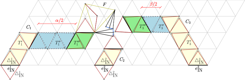
We define three main types of gadgets. A variable $v_{i}\in\phi$ is modeled by means of a gadget we call variable gadget, a clause $c_{j}\in\phi$ by means of a gadget we call a clause gadget, and an edge $(v_{i},c_{j})\in G_{\phi}$ by means of a gadget we call a $k$-transmission gadget. We also define two auxiliary gadgets we call ladder gadgets and flag gadgets. Ladder gadgets are used to provide structural rigidity to the reduction, and flag gadgets are used as an auxiliary tool in the construction of clause gadgets. To construct the gadgets we use the lengths $w_{1}:=1$, $w_{2}:=0.9$, $w_{3}:=0.2$, and $w_{4}:=1.61$. In the figures, we represent edges of length $w_{1},w_{2},w_{3}$, and $w_{4}$ by means of black, red, blue, and green segments, respectively. The lengths $w_{1}$ and $w_{2}$ play a special role in the reduction. We use them to define two main types of triangles: Equilateral triangles with sides of length $w_{1}$, which we call frame triangles, and flat isosceles triangles with base of length $w_{1}$ and two shorter sides of length $w_{2}$, which we call transmission triangles. We refer to the subgraph of a gadget formed by its frame triangles as the frame of the gadget. With the exception of clause gadgets, the frame of every gadget is a maximal outerplanar graph with a unique planar straight-line realization (up to rigid transformations); whereas the frame of a clause gadget consists of three maximal outerplanar graphs. The variable, clause, and $k$-transmission gadgets are constructed in such a way that every frame triangle shares two of its sides each with a different transmission triangle. Since $\frac{w_{1}}{w_{2}}=\frac{1}{0.9}<\sqrt{3}$, by Lemma 2 we have that, in any planar straight-line realization of $H_{\phi}$, two transmission triangles that share a side with a frame triangle cannot both be drawn inside such a frame triangle. This property is exploited in order to propagate along the frame of the gadgets the truth values of each literal; this value is initially determined by the embedding of a transmission triangle inside one or the other of its two incident frame triangles of a variable gadget. A final common property of all our gadgets is a set of special edges we call attachment edges, which are edges of frame triangles that are also edges of transmission triangles. In the figures, attachment edges are represented as thick black segments. We use attachment edges to combine gadgets together so that the encoded truth values can be propagated along the resulting $2$-tree. We exploit properties D1-D7 of $\Gamma^{*}_{\phi}$ to guarantee that, after combining all the gadgets, $H_{\phi}$ has a planar straight-line realization if and only if $\phi$ is satisfiable.

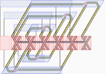
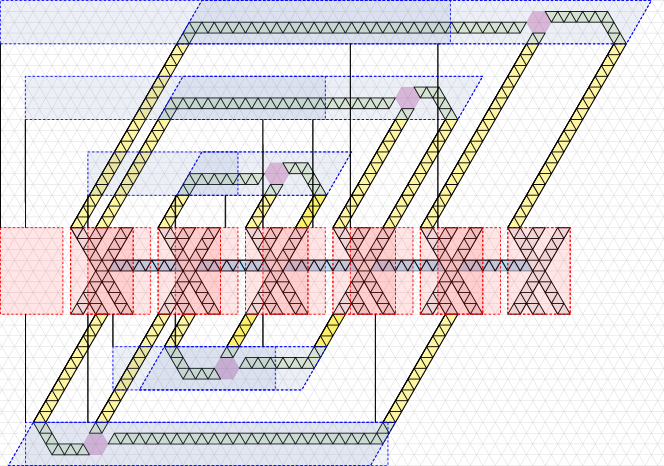
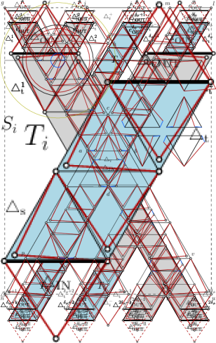
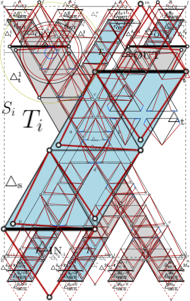
An example of a planar straight-line realization of $H_{\phi}$ is shown in Fig. 7. This example illustrates a high-level sketch of the reduction from $\Gamma^{*}_{\phi}$ to $H_{\phi}$. The grid formed by lines with slope $0^{\circ}$, $60^{\circ}$, and $120^{\circ}$ is shown in light gray. For the sake of clarity, we only show the frames of the gadgets forming $H_{\phi}$. To illustrate the correspondence with the boxes of Fig. 6(b) that represent the variables and clauses of $\phi$, we also show the bounding boxes of the variable gadgets (in dashed red) and the trapezoids enclosing the clause gadgets (in dashed blue). We next provide a high-level description of each gadget.

The variable gadget.

Remember that $\delta_{\phi}$ denotes the maximum degree of $G_{\phi}$. The variable gadget provides $2\delta_{\phi}$ attachment edges. Further, its frame is a maximal outerplanar graph, hence it has a unique planar straight-line realization, up to rigid transformations. Let $\Gamma$ be a planar straight-line realization of the variable gadget, $\Gamma_{f}\subset\Gamma$ be the realization of the frame of the gadget in $\Gamma$, and $B_{f}$ be the bounding box of $\Gamma_{f}$. In Fig. 7, the realization $\Gamma_{f}$ is shaded gray and $B_{f}$ is shown with red dashed lines. Up to a rotation of $\Gamma$, we have that $\delta_{\phi}$ attachment edges lie along the top side of $B_{f}$, say $s_{t}$, while the remaining $\delta_{\phi}$ attachment edges lie along the bottom side of $B_{f}$, say $s_{b}$. The crucial property of the variable gadget is that, in $\Gamma$, either all the transmission triangles incident to attachment edges along $s_{t}$ are drawn outside $\Gamma_{f}$, or all the transmission triangles incident to attachment edges along $s_{b}$ are drawn outside $\Gamma_{f}$. We exploit this property to encode the truth assignment of the variable modeled by the gadget. In particular, the purpose of the attachment edges on $s_{t}$ is to propagate the truth value to incident positive clauses, while the purpose of the attachment edges on $s_{b}$ is to propagate the negated truth value to incident negative clauses.

The ladder gadget.

By Property D3, the bottom sides of the boxes representing variables lie on the same horizontal grid line in $\Gamma^{*}_{\phi}$. Consider the order of appearance of the boxes while traversing such line from left to right. The ladder gadget consists of a sequence of frame triangles that form a maximal outerpath and that connect the frames of two consecutive variable gadgets; see the triangles shaded blue in Fig. 7. The purpose of the ladder gadgets is to make the entire graph $H_{\phi}$ biconnected and to make the union of the frames of all the gadgets a maximal outerplanar graph, which has a unique planar straight-line realization, up to rigid transformations. This realization can then be navigated by the truth values of the variables.

The $k$-transmission gadget.

Let $v_{i}$ and $c_{j}$ be a variable and a clause of $\phi$, respectively, such that $(v_{i},c_{j})$ is an edge of $G_{\phi}$. Let $\mathcal{V}_{i}$ denote the variable gadget modeling $v_{i}$ and $\mathcal{C}_{j}$ denote the clause gadget modeling $c_{j}$. The purpose of the transmission gadget is to “transmit” to $\mathcal{C}_{j}$ the truth value of $v_{i}$ corresponding to the realization of $\mathcal{V}_{i}$. The frame of the $k$-transmission gadget is a sequence of $k$ frame triangles that form a maximal outerpath; see the triangles shaded yellow in Fig. 7. The parameter $k$ coincides with twice the length of the segment representing the edge $(v_{i},c_{j})$ in $\Gamma^{*}_{\phi}$. The $k$-transmission gadget provides two attachment edges, each incident to one of the faces of the frame that correspond to the end-vertices of its dual path. To connect $\mathcal{V}_{i}$ to $\mathcal{C}_{j}$, one of these attachment edges is identified with an attachment edge of $\mathcal{V}_{i}$ and the second one is identified with an attachment edge of $\mathcal{C}_{j}$.

The clause gadget.

Unlike the aforementioned gadgets, the clause gadget consists of three distinct connected components. Two of these components are formed by frame and transmission triangles. The third component is not only formed by frame and transmission triangles, but also by a special subgraph we call a flag gadget. The frame of each component forms a maximal outerpath; see the triangles shaded light green in Fig. 7. The clause gadget contains six attachment edges. Three of them, that we call input attachment edges, are used to combine the clause gadget with the three $k$-transmission gadgets modeling the edges of $G_{\phi}$ incident to the clause. The remaining three, that we call output attachment edges, are used to model the logic of the clause; in particular, one of them connects the frame of a component to the flag gadget.

Consider a positive clause $c_{j}$ that contains the literal $v_{i}$. The clause $c_{j}$ is modeled in $H_{\phi}$ by a clause gadget $\mathcal{C}_{j}$ and is represented in $\Gamma^{*}_{\phi}$ by a trapezoid $t_{j}$. The edge $(v_{i},c_{j})$ of $G_{\phi}$ is modeled in $H_{\phi}$ by a $k$-transmission gadget $\mathcal{T}_{i,j}$ and is represented in $\Gamma^{*}_{\phi}$ by a line segment $s_{i,j}$. The gadgets $\mathcal{C}_{j}$ and $\mathcal{T}_{i,j}$ are combined together by means of an attachment edge $e$ of $\mathcal{T}_{i,j}$ that is identified with an input attachment edge of $\mathcal{C}_{j}$. The combination of $\mathcal{C}_{j}$ with $\mathcal{T}_{i,j}$ exploits the following geometric property. Consider the unique planar straight-line realization of the subgraph of $H_{\phi}$ that is the union of all the ladder gadgets and of the frames of all the variable and transmission gadgets. By Property D5 of $\Gamma^{*}_{\phi}$ and the fact that $k$ coincides with twice the length of $s_{i,j}$, we have that, in such a realization, the attachment edge $e$ is represented by a line segment lying along the bottom side of $t_{j}$. If $c_{j}$ is instead negative, then $e$ lies along the top side of $t_{j}$.

By the geometric property described above, the input attachment edges of the components of $\mathcal{C}_{j}$ are represented by line segments that lie either all on the bottom or all on the top side of $t_{j}$. The frames of the components of $\mathcal{C}_{j}$ can thus be defined so that, in any planar straight-line realization of $\mathcal{C}_{j}$, we have that (i) all the frames are entirely contained in $t_{j}$ and (ii) the output attachment edges are represented by line segments that are “close” to each other. In Fig. 7, we emphasize this closeness by depicting a pink-shaded hexagon whose vertices coincide with some of the endpoints of these line segments.

Consider the transmission triangles incident to the output attachment edges of the components of $\mathcal{C}_{j}$. The clause gadget admits a planar straight-line realization if and only if at least one of these transmission triangles is drawn inside its incident frame triangle. Let $C$ be a component of $\mathcal{C}_{j}$. Assume again that the input attachment edge of $C$ is shared with a $k$-transmission gadget $\mathcal{T}_{i,j}$ that connects $\mathcal{C}_{j}$ to the variable gadget representing a variable $v_{i}$. Our gadgets guarantee that, in any planar straight-line realization of $H_{\phi}$, the transmission triangle incident to the output attachment edge of $C$ can be drawn inside its adjacent frame triangle only if the gadget modeling $v_{i}$ represents the value False (resp. True) and $c_{j}$ is positive (resp. negative). Thus, if all three variables appearing in $c_{j}$ represent the value False (resp. True) and $c_{j}$ is positive (resp. negative), then $H_{\phi}$ admits no planar straight-line realization. Conversely, if at least one of the variables appearing in $c_{j}$ represents the value True (resp. False) and $c_{i}$ is positive (resp. negative), then the transmission triangle of the corresponding component of $\mathcal{C}_{j}$ can be drawn inside its incident frame triangle so that $\mathcal{C}_{j}$ admits a planar straight-line realization.

4.3 Description of the gadgets

We now present complete constructions for the following gadgets: The transmission gadget, the split gadget, the variable gadget, the flag gadget, and the clause gadget. We will later show how to precisely combine these gadgets to obtain $H_{\phi}$.

In the following, whenever we combine two gadgets $G_{1}$ and $G_{2}$, we proceed as follows. First, we identify one attachment edge of $G_{1}$ with one attachment edge of $G_{2}$ to obtain a single edge $e$ that belongs to both $G_{1}$ and $G_{2}$. Second, we remove the degree-$2$ vertex of any of the two transmission triangles sharing the edge $e$, together with the two edges incident to such vertex. This operation always results in a $2$-tree, as a consequence of the following lemma.

Lemma 5.

Let $G_{1}$ and $G_{2}$ be two $2$-trees, and let $e_{1}$ be an edge of $G_{1}$ and $e_{2}$ be an edge of $G_{2}$. The graph $G$ obtained from $G_{1}$ and $G_{2}$ by identifying $e_{1}$ and $e_{2}$ is a $2$-tree.

Proof.

We prove the statement by induction on $|V(G_{2})|$.

In the base case, $|V(G_{2})|=3$, that is, $G_{2}$ is a $3$-cycle. Then $G$ is obtained by adding to $G_{1}$ a vertex $v$ and two edges $(v,u)$ and $(v,w)$, where $u$ and $w$ are the end-vertices of $e_{1}$. Hence $G$ is a $2$-tree.

In the inductive case, let $v$ be a degree-$2$ vertex of $G_{2}$ that is different from both the end-vertices of $e_{2}$. This vertex exists by Property (P3) of a $2$-tree. Let $u$ and $w$ be the neighbors of $v$ in $G_{2}$. By Property (P2) of a $2$-tree, we have that $(u,w)$ is an edge of $G_{2}$. Let $G^{\prime}_{2}$ be the graph obtained from $G_{2}$ by removing $v$ and its incident edges $(v,u)$ and $(v,w)$; note that $e_{2}$ is an edge of $G^{\prime}_{2}$. By induction, the graph $G^{\prime}$ obtained from $G_{1}$ and $G^{\prime}_{2}$ by identifying $e_{1}$ and $e_{2}$ is a $2$-tree. Then $G$ is obtained by adding to $G^{\prime}$ the vertex $v$ and the edges $(v,u)$ and $(v,w)$; since $G^{\prime}$ contains the edge $(u,w)$, it follows that $G$ is a $2$-tree. ∎

The $k$-transmission gadget.

(a)

(b)

Figure 8: Illustration of two $k$-transmission gadgets (in (a) and in (b)), differing from one another for the choice of the attachment edge belonging to $\triangle_{t}$. For each of the two $k$-transmission gadgets, both a planar straight-line realization in which $\triangle_{\textrm{IN}}$ is drawn inside $\triangle_{s}$ and a planar straight-line realization in which $\triangle_{\textrm{OUT}}$ is draw inside $\triangle_{t}$ are shown. In these illustrations, we have $k=4$.

For any positive even integer $k$, a $k$-transmission gadget consists of a sequence $\triangle_{s}=\triangle_{1},\dots,\triangle_{k}=\triangle_{t}$ of $k$ frame triangles, in which each triangle shares exactly one edge with its successor; refer to Fig. 8. For each pair of consecutive frame triangles, we insert a transmission triangle (solid red triangles in Fig. 8) whose base edge we identify with the common edge between the frame triangles. When the value $k$ is not relevant, we refer to a $k$-transmission gadget simply as a “transmission gadget”. A $k$-transmission gadget provides two attachment edges. The first attachment edge, which we denote $e_{\textrm{IN}}$, can be selected as any of the two edges of $\triangle_{s}$ that is not shared with its successor frame triangle. Similarly, the second attachment edge, which we denote $e_{\textrm{OUT}}$, can be selected as any of the two edges of $\triangle_{t}$ that is not shared with its predecessor frame triangle. This yields four possible $k$-transmission gadgets. We complete the construction of a transmission gadget by inserting a transmission triangle $\triangle_{\textrm{IN}}$ whose base we identify with $e_{\textrm{IN}}$, and a transmission triangle $\triangle_{\textrm{OUT}}$ whose base we identify with $e_{\textrm{OUT}}$; see the dashed triangles in Fig. 8.

Clearly, a transmission gadget is a $2$-tree and its frame is a maximal outerpath. In any planar straight-line realization of a transmission gadget, its attachment edges are either parallel or not. In the first case, we say that the transmission gadget is straight, whereas in the second case we say that it is turning; the transmission gadgets in LABEL:fig:transmission_gadget-a and LABEL:fig:transmission_gadget-b are straight and turning, respectively. We have the following lemma.

Lemma 6.

In any planar straight-line realization of a transmission gadget, if $\triangle_{\textrm{IN}}$ is drawn inside $\triangle_{s}$, then $\triangle_{\textrm{OUT}}$ is drawn outside $\triangle_{t}$. Further, if $\triangle_{\textrm{OUT}}$ is drawn inside $\triangle_{t}$, then $\triangle_{\textrm{IN}}$ is drawn outside $\triangle_{s}$.

Proof.

Consider the sequence $\triangle_{1},\dots,\triangle_{k}$ of frame triangles of a transmission gadget, where $\triangle_{s}=\triangle_{1}$ and $\triangle_{t}=\triangle_{k}$. For $i=1,\dots,k-1$, the triangles $\triangle_{i}$ and $\triangle_{i+1}$ share a single edge, which is the base of a transmission triangle we denote with $\triangle^{T}_{i}$.

We only prove the first part of the statement, since the second part is symmetric. Consider any planar straight-line realization of a transmission gadget in which $\triangle_{\textrm{IN}}$ is drawn inside $\triangle_{s}$. Since $\frac{w_{1}}{w_{2}}=\frac{1}{0.9}<\sqrt{3}$, by Lemma 2 we have that $\triangle_{\textrm{IN}}$ and $\triangle^{T}_{1}$ are not both drawn inside $\triangle_{1}=\triangle_{s}$; therefore $\triangle^{T}_{1}$ is drawn inside $\triangle_{2}$. Similarly, since $\triangle^{T}_{i}$ is drawn inside $\triangle_{i+1}$, then $\triangle^{T}_{i+1}$ is drawn inside $\triangle_{i+2}$ for $i=1,\dots,k-2$. Finally, since $\triangle^{T}_{k-1}$ is drawn inside $\triangle_{k}=\triangle_{t}$, we have that $\triangle_{\textrm{OUT}}$ is drawn outside $\triangle_{t}$. ∎

The split gadget.

(a)

(b)

(c)

(d)

Figure 9: Split gadget construction. (a) The $4$-transmission gadgets $T^{1}$ and $T^{2}$. (b) The gadgets $T^{1}$ and $T^{2}$ after replacing $\triangle^{\prime}_{1}$ and $\triangle^{\prime}_{2}$ with scalene triangles. (c) The split gadget with $\triangle_{\textrm{IN}}$ drawn inside $\triangle_{s}$. (d) The split gadget with $\triangle^{i}_{\textrm{OUT}}$ drawn inside $\triangle^{i}_{t}$, for $i=1,2$.

Let $T^{1}$ and $T^{2}$ be two straight $4$-transmission gadgets. The split gadget can be obtained from $T^{1}$ and $T^{2}$ as follows. For $i=1,2$, let us denote the triangles $\triangle_{\textrm{IN}}$, $\triangle_{\textrm{OUT}}$, $\triangle_{s}$, and $\triangle_{t}$ of $T^{i}$ as $\triangle^{i}_{\textrm{IN}}$, $\triangle^{i}_{\textrm{OUT}}$, $\triangle^{i}_{s}$, and $\triangle^{i}_{t}$, respectively, and the attachment edges $e_{\textrm{IN}}$ and $e_{\textrm{OUT}}$ of $T^{i}$ as $e^{i}_{\textrm{IN}}$ and $e^{i}_{\textrm{OUT}}$, respectively; see LABEL:fig:split_gadget-a. For $i=1,2$, let $\triangle^{\prime}_{i}$ be the transmission triangle of $T^{i}$ that is incident to the frame triangle $\triangle^{i}_{s}$ and different from $\triangle^{i}_{\textrm{IN}}$. First, we replace $\triangle^{\prime}_{i}$ with a scalene triangle, which we still refer to as $\triangle^{\prime}_{i}$, whose longest side is shared with $\triangle^{i}_{s}$ and whose two shorter sides have length $w_{2}$ and $w_{3}$; refer to LABEL:fig:split_gadget-b. After this replacement, we still denote the “modified” transmission gadgets as $T^{1}$ and $T^{2}$. Finally, we identify the frame triangles $\triangle^{1}_{s}$ and $\triangle^{2}_{s}$ to obtain a single frame triangle we denote with $\triangle_{s}$, and we identify the transmission triangles $\triangle^{1}_{\textrm{IN}}$ and $\triangle^{2}_{\textrm{IN}}$ to obtain a single transmission triangle we denote with $\triangle_{\textrm{IN}}$; refer to LABEL:fig:split_gadget-c and LABEL:fig:split_gadget-d. By Lemma 5 and the fact that the transmission gadgets are $2$-trees, we have that the split gadget is a $2$-tree and its frame is a maximal outerpath.

The split gadget provides three attachment edges. Namely, the attachment edge $e_{\textrm{IN}}$ incident to $\triangle_{\textrm{IN}}$ (obtained by identifying $e^{1}_{\textrm{IN}}$ and $e^{2}_{\textrm{IN}}$), the attachment edge $e^{1}_{\textrm{OUT}}$ incident to $\triangle^{1}_{\textrm{OUT}}$, and the attachment edge $e^{2}_{\textrm{OUT}}$ incident to $\triangle^{2}_{\textrm{OUT}}$. We have the following property.

Property 2.

The scalene triangles $\triangle^{\prime}_{1}$ and $\triangle^{\prime}_{2}$ satisfy the following properties.

1. The triangles $\triangle^{\prime}_{1}$ and $\triangle^{\prime}_{2}$ can be drawn together inside $\triangle_{s}$ without intersecting each other.

2. Neither $\triangle^{\prime}_{1}$ nor $\triangle^{\prime}_{2}$ can be drawn together with $\triangle_{\textrm{IN}}$ inside $\triangle_{s}$ without intersecting each other.

Proof.

Statement (a) follows from the fact that the angles of $\triangle^{\prime}_{1}$ and $\triangle^{\prime}_{2}$ incident to the vertex they share sum up to less than $60^{\circ}$. Indeed, by the law of the cosines, such angles are equal to $\arccos\left({\frac{w_{1}^{2}+w_{2}^{2}-w_{3}^{2}}{2w_{1}w_{2}}}\right)<\arccos(0.983)<11^{\circ}$.

Statement (b) follows from the fact that, for $i=1,2$, the angles of $\triangle^{\prime}_{i}$ and $\triangle_{\textrm{IN}}$ incident to the vertex they share sum up to more than $60^{\circ}$. Indeed, by the law of the cosines, such angles are equal to $\arccos\left({\frac{w_{1}^{2}+w_{3}^{2}-w_{2}^{2}}{2w_{1}w_{3}}}\right)>\arccos(0.57)>54^{\circ}$ and $\arccos\left({\frac{w_{1}}{2w_{2}}}\right)>\arccos(0.56)>55^{\circ}$, respectively. ∎

Using Property 2, the proof of Lemma 6 can be easily adapted to obtain the following.

Lemma 7.

In any planar straight-line realization of the split gadget, if $\triangle_{\textrm{IN}}$ is drawn inside $\triangle_{s}$, then $\triangle^{1}_{\textrm{OUT}}$ is drawn outside $\triangle^{1}_{t}$ and $\triangle^{2}_{\textrm{OUT}}$ is drawn outside $\triangle^{2}_{t}$. Further, if $\triangle^{1}_{\textrm{OUT}}$ is drawn inside $\triangle^{1}_{t}$ or $\triangle^{2}_{\textrm{OUT}}$ is drawn inside $\triangle^{2}_{t}$, then $\triangle_{\textrm{IN}}$ is drawn outside $\triangle_{s}$.

The variable gadget.

Remember that $\delta_{\phi}$ denotes the maximum degree of $G_{\phi}$. Let $S_{1},S_{2},\dots,S_{2\delta_{\phi}-2}$ be $2\delta_{\phi}-2$ split gadgets, and $T_{2},T_{3},\dots,T_{2\delta_{\phi}-3}$ be $2\delta_{\phi}-4$ straight transmission gadgets such that, for $i=2,\dots,\delta_{\phi}-1$, the gadgets $T_{i}$ and $T_{2\delta_{\phi}-i-1}$ are $4(i-1)$-transmission gadgets. The variable gadget can be obtained by combining these gadgets as follows; refer to Fig. 10.

Figure 10: Schema of the variable gadget when the maximum degree $\delta_{\phi}$ of $G_{\phi}$ is $4$.

• For $i=1,\dots,\delta_{\phi}-2$, we combine $S_{i}$ and $S_{i+1}$ by identifying the attachment edge $e_{\textrm{IN}}$ of $S_{i}$ with the attachment edge $e^{1}_{\textrm{OUT}}$ of $S_{i+1}$;

• we combine $S_{\delta_{\phi}-1}$ and $S_{\delta_{\phi}}$ by identifying the attachment edge $e_{\textrm{IN}}$ of $S_{\delta_{\phi}-1}$ with the attachment edge $e_{\textrm{IN}}$ of $S_{\delta_{\phi}}$;

• for $i=\delta_{\phi},\dots,2\delta_{\phi}-3$, we combine $S_{i}$ and $S_{i+1}$ by identifying the attachment edge $e^{1}_{\textrm{OUT}}$ of $S_{i}$ with the attachment edge $e_{\textrm{IN}}$ of $S_{i+1}$; and

• for $i=2,\dots,2\delta_{\phi}-3$, we combine $S_{i}$ and $T_{i}$ by identifying the attachment edge $e^{2}_{\textrm{OUT}}$ of $S_{i}$ with the attachment edge $e_{\textrm{IN}}$ of $T_{i}$.

By Lemma 5 and the fact that transmission and split gadgets are $2$-trees, we have that the variable gadget is a $2$-tree and its frame is a maximal outerplanar graph.

The variable gadget provides $2\delta_{\phi}$ attachment edges; refer to Fig. 11. Namely:

• the attachment edges $e^{1}_{\textrm{OUT}}$ and $e^{2}_{\textrm{OUT}}$ of $S_{1}$,

• for $i=2,\dots,2\delta_{\phi}-3$, the attachment edge $e_{\textrm{OUT}}$ of $T_{i}$, which we denote as $e^{i+1}_{\textrm{OUT}}$, and

• the attachment edges $e^{1}_{\textrm{OUT}}$ and $e^{2}_{\textrm{OUT}}$ of $S_{2\delta_{\phi}-2}$, which we denote as $e^{2\delta_{\phi}-1}_{\textrm{OUT}}$ and $e^{2\delta_{\phi}}_{\textrm{OUT}}$, respectively.

For $i=1,\dots,2\delta_{\phi}$, we also denote by $\triangle^{i}_{\textrm{OUT}}$ and by $\triangle^{i}_{t}$ the transmission triangle and the frame triangle incident to $e^{i}_{\textrm{OUT}}$, respectively. Finally, let $\triangle_{\textrm{IN}}$ be the transmission triangle that is incident to the attachment edge shared by the split gadgets $S_{\delta_{\phi}-1}$ and $S_{\delta_{\phi}}$. We call $\triangle_{\textrm{IN}}$ the truth-assignment triangle. Intuitively, the truth value associated with a planar straight-line realization of the variable gadget, will depend on whether $\triangle_{\textrm{IN}}$ lies inside the frame triangle $\triangle_{s}$ of $S_{\delta_{\phi}-1}$ or inside the frame triangle $\triangle_{s}$ of $S_{\delta_{\phi}}$ in such a realization. We show the following simple and yet useful geometric property of the variable gadget.

Property 3.

In any planar straight-line realization of the variable gadget, up to a rotation, the frame lies in an axis-aligned box $B$ of width $w_{1}(2\delta_{\phi}-1)$ and height $2\sqrt{3}w_{1}(\delta_{\phi}-1)$. Furthermore, the attachment edges $e^{1}_{\textrm{OUT}},\dots,e^{\delta_{\phi}}_{\textrm{OUT}}$ lie along the top side of $B$ at distance $w_{1}$ from each other, and the attachment edges $e^{\delta_{\phi}+1}_{\textrm{OUT}},\dots,e^{2\delta_{\phi}}_{\textrm{OUT}}$ lie along the bottom side of $B$ at distance $w_{1}$ from each other.

We have the following lemma. Refer to Fig. 11.

(a)

(b)

Figure 11: The variable gadget when the maximum degree $\delta_{\phi}$ of $G_{\phi}$ is $4$. In the logic of the reduction, the realization on the left corresponds to an assignment of True to the variable represented by the variable gadget, while the realization on the right corresponds to an assignment of False to the variable represented by the variable gadget.

Lemma 8.

In any planar straight-line realization of the variable gadget, if the truth-assignment triangle $\triangle_{\textrm{IN}}$ is drawn inside the frame triangle $\triangle_{s}$ of $S_{\delta_{\phi}-1}$ (resp. of $S_{\delta_{\phi}}$), then, for $i=1,\dots,\delta_{\phi}$ (resp. for $i=\delta_{\phi}+1,\dots,2\delta_{\phi}$), the transmission triangle $\triangle^{i}_{\textrm{OUT}}$ is drawn outside the frame triangle $\triangle^{i}_{t}$. Furthermore, if there is some $i\in\{1,\dots,\delta_{\phi}\}$ (resp. some $i\in\{\delta_{\phi}+1,\dots,2\delta_{\phi}\}$) for which the transmission triangle $\triangle^{i}_{\textrm{OUT}}$ is drawn inside the frame triangle $\triangle^{i}_{t}$, then $\triangle_{\textrm{IN}}$ is drawn inside the frame triangle $\triangle_{s}$ of $S_{\delta_{\phi}}$ (resp. of $S_{\delta_{\phi}-1}$).

Proof.

We start with the first part of the statement. Let $\Gamma$ be a planar straight-line realization of the variable gadget. Suppose the truth-assignment triangle $\triangle_{\textrm{IN}}$ is drawn inside the frame triangle $\triangle_{s}$ of $S_{\delta_{\phi}-1}$ in $\Gamma$. We show that, for $i=1,\dots,\delta_{\phi}$, the transmission triangle $\triangle^{i}_{\textrm{OUT}}$ is drawn outside the frame triangle $\triangle^{i}_{t}$ in $\Gamma$. By a symmetric argument we can proof that, if $\triangle_{\textrm{IN}}$ is drawn inside the frame triangle $\triangle_{s}$ of $S_{\delta_{\phi}}$ in $\Gamma$, then, for $i=\delta_{\phi},\dots,2\delta_{\phi}$, the transmission triangle $\triangle^{i}_{\textrm{OUT}}$ is drawn outside the frame triangle $\triangle^{i}_{t}$ in $\Gamma$. We have the following claims.

Claim 1.

Consider any two split gadgets $S_{i}$ and $S_{i-1}$, for $i=\delta_{\phi}-1,\dots,2$. If the transmission triangle $\triangle^{1}_{\textrm{OUT}}$ of $S_{i}$ is drawn outside the frame triangle $\triangle^{1}_{t}$ of $S_{i}$, then the transmission triangle $\triangle^{1}_{\textrm{OUT}}$ of $S_{i-1}$ is drawn outside the frame triangle $\triangle^{1}_{t}$ of $S_{i-1}$.

Proof.

Observe that, if the transmission triangle $\triangle^{1}_{\textrm{OUT}}$ of $S_{i}$ is drawn outside the frame triangle $\triangle^{1}_{t}$ of $S_{i}$, then it lies inside the frame triangle $\triangle_{s}$ of $S_{i-1}$. Since the transmission triangle $\triangle^{1}_{\textrm{OUT}}$ is in fact a copy of the transmission triangle $\triangle_{IN}$ of $S_{i-1}$ (which has been removed when combining $S_{i}$ and $S_{i-1}$), by Lemma 7 we have that the transmission triangle $\triangle^{1}_{\textrm{OUT}}$ of $S_{i-1}$ is drawn outside the frame triangle $\triangle^{1}_{t}$ of $S_{i-1}$. ∎

Claim 2.

Consider any split gadget $S_{i}$ and any transmission gadget $T_{i}$, for $i=\delta_{\phi}-1,\dots,2$. If the transmission triangle $\triangle^{2}_{\textrm{OUT}}$ of $S_{i}$ is drawn outside the frame triangle $\triangle^{2}_{t}$ of $S_{i}$, then the transmission triangle $\triangle_{\textrm{OUT}}$ of $T_{i}$ is drawn outside the frame triangle $\triangle_{t}$ of $T_{i}$.

Proof.

Observe that, if the transmission triangle $\triangle^{2}_{\textrm{OUT}}$ of $S_{i}$ is drawn outside the frame triangle $\triangle^{2}_{t}$ of $S_{i}$, then it lies inside the frame triangle $\triangle_{s}$ of $T_{i}$. Since $\triangle^{2}_{\textrm{OUT}}$ is in fact a copy of the transmission triangle $\triangle_{IN}$ of $T_{i}$ (which has been removed when combining $S_{i}$ and $T_{i}$), by Lemma 6 we have that the transmission triangle $\triangle_{\textrm{OUT}}$ of $T_{i}$ is drawn outside the frame triangle $\triangle_{t}$ of $T_{i}$. ∎

Since the truth-assignment triangle $\triangle_{\textrm{IN}}$ lies inside the frame triangle $\triangle_{s}$ of $S_{\delta_{\phi}-1}$, then by Lemma 7, the transmission triangles $\triangle^{1}_{\textrm{OUT}}$ and $\triangle^{2}_{\textrm{OUT}}$ of $S_{\delta_{\phi}-1}$ are drawn outside the frame triangles $\triangle^{1}_{t}$ and $\triangle^{2}_{t}$ of $S_{\delta_{\phi}-1}$, respectively. Hence, in the variable gadget, the transmission triangle $\triangle^{i}_{\textrm{OUT}}$ is drawn outside the frame triangle $\triangle^{i}_{t}$; this follows from Claim 1 for $i=1,2$, and from Claim 2 for $i=3,\dots,\delta_{\phi}$.

We now prove the second part of the statement. Let $\Gamma$ be a planar straight-line realization of the variable gadget. Suppose that, for some $j\in\{1,\ldots,\delta_{\phi}\}$, there is a transmission triangle $\triangle^{j}_{\textrm{OUT}}$ of the variable gadget drawn inside the frame triangle $\triangle^{j}_{t}$ of the variable gadget. We show that the truth-assignment triangle $\triangle_{\textrm{IN}}$ is drawn inside the frame triangle $\triangle_{s}$ of $S_{\delta_{\phi}}$ in $\Gamma$. By a symmetric argument we can proof that, if there is some $j\in\{\delta_{\phi}+1,\dots,2\delta_{\phi}\}$ for which a transmission triangle $\triangle^{j}_{\textrm{OUT}}$ of the variable gadget is drawn inside the frame triangle $\triangle^{j}_{t}$ of the variable gadget, then the truth-assignment triangle $\triangle_{\textrm{IN}}$ is drawn inside the frame triangle $\triangle_{s}$ of $S_{\delta_{\phi-1}}$ in $\Gamma$. We have the following two claims, whose proofs are symmetric to the proofs of Claims 1 and 2.

Claim 3.

Consider any two split gadgets $S_{i}$ and $S_{i-1}$, for $i=\delta_{\phi}-1,\dots,2$. If the transmission triangle $\triangle^{1}_{\textrm{OUT}}$ of $S_{i-1}$ is drawn inside the frame triangle $\triangle^{1}_{t}$ of $S_{i-1}$, then the transmission triangle $\triangle^{1}_{\textrm{OUT}}$ of $S_{i}$ is drawn inside the frame triangle $\triangle^{1}_{t}$ of $S_{i}$.

Claim 4.

Consider any split gadget $S_{i}$ and any transmission gadget $T_{i}$, for $i=\delta_{\phi}-1,\dots,2$. If the transmission triangle $\triangle_{\textrm{OUT}}$ of $T_{i}$ is drawn inside the frame triangle $\triangle_{t}$ of $T_{i}$, then the transmission triangle $\triangle^{2}_{\textrm{OUT}}$ of $S_{i}$ is drawn inside the frame triangle $\triangle^{2}_{t}$ of $S_{i}$.

If $1\leq j\leq 2$, then the transmission triangle $\triangle^{j}_{\textrm{OUT}}$ of the variable gadget is actually a transmission triangle of the split gadget $S_{1}$. Hence, by Claim 3, we have that the transmission triangle $\triangle^{1}_{\textrm{OUT}}$ of $S_{\delta_{\phi}-1}$ is drawn inside the frame triangle $\triangle^{1}_{t}$ of $S_{\delta_{\phi}-1}$. If instead $3\leq j\leq\delta_{\phi}$, then the transmission triangle $\triangle^{j}_{\textrm{OUT}}$ of the variable gadget is actually a transmission triangle of a transmission gadget. Hence, by Claim 4, we have that the transmission triangle $\triangle^{2}_{\textrm{OUT}}$ of $S_{j}$ is drawn inside the frame triangle $\triangle^{2}_{t}$ of $S_{j}$. This fact and again Claim 3 imply that either the transmission triangle $\triangle^{1}_{\textrm{OUT}}$ of $S_{\delta_{\phi}-1}$ is drawn inside the frame triangle $\triangle^{1}_{t}$ of $S_{\delta_{\phi}-1}$ (which happens when $j<\delta_{\phi}$), or the transmission triangle $\triangle^{2}_{\textrm{OUT}}$ of $S_{\delta_{\phi}-1}$ is drawn inside the frame triangle $\triangle^{2}_{t}$ of $S_{{\delta_{\phi}}-1}$ (which happens when $j=\delta_{\phi}$). In all cases, by Lemma 7, the truth-assignment triangle $\triangle_{\textrm{IN}}$ is drawn inside the frame triangle $\triangle_{s}$ of $S_{\delta_{\phi}}$ in $\Gamma$. ∎

Figure 12: The triangles $(a,b,c)$, $(d,b,c)$, $(g,d,c)$, and $(g,h,c)$ of the flag gadget.

The flag gadget.

The flag gadget consists of the following triangles (see Figs. 13 and 12):

1. a transmission triangle $(a,b,c)$ with base $(b,c)$,

2. a tall isosceles triangle $(d,b,c)$ with base $(b,c)$ of length $w_{1}$ and two longer sides of length $w_{4}$,

3. a flat isosceles triangle $(f,d,c)$ with base $(d,c)$ of length $w_{4}$ and two shorter sides of length $w_{2}$,

4. an equilateral triangle $(g,d,c)$ with sides of length $w_{4}$,

5. a flat isosceles triangle $(h,g,c)$ with base $(g,c)$ of length $w_{4}$ and two shorter sides of length $w_{1}$,

6. four tall isosceles triangles $(h,i,g)$, $(i,l,g)$, $(h,m,c)$, and $(m,n,c)$ with bases $(h,i)$, $(i,l)$, $(h,m)$, and $(m,n)$, respectively, of length $w_{3}$ and two longer sides of length $w_{1}$.

By Lemma 5 and the fact that any two of the listed triangles share at most one edge, we have that the flag gadget is a $2$-tree. The flag gadget provides a single attachment edge, which coincides with the base $(b,c)$ of the transmission triangle $(a,b,c)$.

(a)

(b)

(c)

Figure 13: The flag gadget and three planar straight-line realizations of it. In (a) and (b) the transmission triangle $(a,b,c)$ lies inside the triangle $(d,b,c)$, while in (c) it lies outside $(d,b,c)$. In (a) the isosceles triangles $(h,m,c)$ and $(m,n,c)$ lie inside $(h,g,c)$, in (b) the isosceles triangles $(h,i,g)$ and $(i,l,g)$ lie inside $(h,g,c)$, and in (c) all four the isosceles triangles $(h,m,c)$, $(m,n,c)$, $(h,m,c)$, and $(m,n,c)$ lie inside $(h,g,c)$.

We will exploit the following geometric properties of the flag gadget.

Property 4.

The flag gadget admits, among others, planar straight-line realizations in which:

1. The triangle $(a,b,c)$ lies inside the triangle $(d,b,c)$, and the triangles $(h,m,c)$ and $(m,n,c)$ lie inside the triangle $(h,g,c)$; see LABEL:fig:flag_gadget-a.

2. The triangle $(a,b,c)$ lies inside the triangle $(d,b,c)$, and the triangles $(h,i,g)$ and $(i,l,g)$ lie inside the triangle $(h,g,c)$; see LABEL:fig:flag_gadget-b.

3. The triangle $(a,b,c)$ lies outside the triangle $(d,b,c)$ and the triangles $(h,m,c)$, $(m,n,c)$, $(h,m,c)$, and $(m,n,c)$ lie inside the triangle $(h,g,c)$; see LABEL:fig:flag_gadget-c.

Property 5.

The values of some relevant angles of the triangles forming the flag gadget are the following:

• $\widehat{bcd}:=\arccos{\frac{w_{1}}{2w_{4}}}=\arccos{\frac{1}{3.22}}\simeq 71.91^{\circ}$

• $\widehat{bca}:=\arccos{\frac{w_{1}}{2w_{2}}}=\arccos{\frac{1}{1.8}}\simeq 56.25^{\circ}$

• $\widehat{fcd}:=\arccos{\frac{w_{4}}{2w_{2}}}=\arccos{\frac{1.61}{1.8}}\simeq 26.56^{\circ}$

• $\widehat{hcg}:=\arccos{\frac{w_{4}}{2w_{1}}}=\arccos{\frac{1.61}{2}}\simeq 36.39^{\circ}$

• $\widehat{chg}:=180^{\circ}-2\cdot\widehat{hcg}\simeq 107.22^{\circ}$

• $\widehat{chm}:=\arccos{\frac{w_{3}}{2w_{1}}}=\arccos{\frac{0.2}{2}}\simeq 84.26^{\circ}$

• Let $\lambda$ be the smallest internal angle of the tall isosceles triangles with two sides of length $w_{1}$ and one side of length $w_{3}$. We have $\lambda=180^{\circ}-2\cdot\widehat{chm}\simeq 180^{\circ}-2\cdot 84.26^{\circ}=11.48^{\circ}$.

We show the following.

Lemma 9.

In any planar straight-line realization of the flag gadget, the following statements hold true:

1. If the transmission triangle $(a,b,c)$ is drawn inside the triangle $(d,b,c)$, then the triangle $(h,g,c)$ is drawn outside the triangle $(g,d,c)$.

2. Not both the vertices $l$ and $n$ lie inside the triangle $(h,g,c)$.

Proof.

Consider a planar straight-line realization of the flag gadget. By Properties b and c of Lemma 1, in such a realization the triangles $(d,b,c)$ and $(g,d,c)$ are not drawn inside one another. Hence, the triangle $(f,d,c)$ lies inside $(d,b,c)$ if and only if it lies outside $(g,d,c)$.

To prove statement (a), suppose the triangle $(a,b,c)$ is drawn inside the triangle $(d,b,c)$. By our discussion above and the fact that $\widehat{fcd}+\widehat{bca}>\widehat{bcd}$, then the triangle $(f,d,c)$ lies inside $(g,d,c)$. By this fact and the fact that $\widehat{fcd}+\widehat{hcg}>\widehat{dcg}=60^{\circ}$, we have that the triangle $(h,g,c)$ is drawn outside $(g,d,c)$. This ends the proof of statement (a).

To prove statement (b) it suffices to show that $m$ and $i$ cannot both lie inside the triangle $(h,g,c)$. This follows from the fact that $\widehat{chm}=\widehat{ghi}$ and $2\cdot\widehat{chm}>\widehat{chg}$. ∎

Figure 14: The $(\alpha,\beta)$-clause gadget with $\alpha=4$ and $\beta=2$.

The clause gadget.

We now describe the construction of the clause gadget. Such a construction is parametric with respect to the distances between the attachment edges of the transmission gadgets coming from the variable gadgets whose literals appear in the clause. By Property D7 and since the attachment edges of the transmission gadgets have length one, the horizontal distance between the two leftmost attachment edges is $\frac{\alpha}{2}+2$, for some non-negative even integer value $\alpha$, and the horizontal distance between the two rightmost attachment edges is $\frac{\beta}{2}+3$, for some non-negative even integer value $\beta$. Based on the values $\alpha$ and $\beta$, we define the clause gadget, which we refer to as the $(\alpha,\beta)$-clause gadget. The gadget provides three attachment edges $e^{1}_{\textrm{IN}}$, $e^{2}_{\textrm{IN}}$, and $e^{3}_{\textrm{IN}}$ incident to the transmission triangles $\triangle^{1}_{\textrm{IN}}$, $\triangle^{2}_{\textrm{IN}}$, and $\triangle^{3}_{\textrm{IN}}$, respectively. The attachment edges $e^{1}_{\textrm{IN}}$, $e^{2}_{\textrm{IN}}$, and $e^{3}_{\textrm{IN}}$ are identified with the attachment edges of the transmission gadgets coming from the variable gadgets whose literals appear in the clause. Also, recall that the transmission triangles $\triangle^{1}_{\textrm{IN}}$, $\triangle^{2}_{\textrm{IN}}$, and $\triangle^{3}_{\textrm{IN}}$ are identified with the ones of the transmission gadgets coming from the variable gadgets whose literals appear in the clause. In any planar straight-line realization of $H_{\phi}$, the edges $e^{1}_{\textrm{IN}}$, $e^{2}_{\textrm{IN}}$, $e^{3}_{\textrm{IN}}$ lie in this left-to-right order along the same horizontal line.

We now describe the $(\alpha,\beta)$-clause gadget for a positive clause (the negative clause has a symmetric construction); refer to Fig. 14. We exploit the placement of $e^{1}_{\textrm{IN}}$, $e^{2}_{\textrm{IN}}$, $e^{3}_{\textrm{IN}}$ (which is fixed, since such edges belong to the union of the frames of the variable, ladder, and transmission gadgets) as a reference for arranging the gadget components. The $(\alpha,\beta)$-clause gadget consists of three subgraphs $C_{1}$, $C_{2}$, and $C_{3}$ defined as follows.

• The subgraph $C_{1}$ is obtained by combining into a single connected component a turning $4$-transmission gadget $T^{\prime}_{1}$, a straight $\alpha$-transmission gadget $T^{\prime\prime}_{1}$, a turning $2$-transmission gadget $T^{\prime\prime\prime}_{1}$, and a flag gadget $F$, as shown in Fig. 14. The attachment edge $e_{\textrm{IN}}$ of $T^{\prime}_{1}$ is the attachment edge $e^{1}_{\textrm{IN}}$ of the clause gadget.

• The subgraph $C_{2}$ is a straight $2$-transmission gadget, whose attachment edge $e_{\textrm{IN}}$ is the attachment edge $e^{2}_{\textrm{IN}}$ of the clause gadget.

• The subgraph $C_{3}$ is obtained by combining into a single connected component a turning $6$-transmission gadget $T^{\prime}_{3}$, a straight $\beta$-transmission gadget $T^{\prime\prime}_{3}$, and a straight $2$-transmission gadget $T^{\prime\prime\prime}_{3}$, as depicted in Fig. 14. The attachment edge $e_{\textrm{IN}}$ of $T^{\prime}_{3}$ is the attachment edge $e^{3}_{\textrm{IN}}$ of the clause gadget.

By Lemma 5 and the fact that transmission and flag gadgets are $2$-trees, we have that each of $C_{1}$, $C_{2}$, and $C_{3}$ is a $2$-tree. We say that a straight-line realization of the $(\alpha,\beta)$-clause gadget is feasible, if it satisfies the following properties:

1. the attachment edges $e^{1}_{\textrm{IN}}$, $e^{2}_{\textrm{IN}}$, and $e^{3}_{\textrm{IN}}$ lie in this left-to-right order on a horizontal line $\ell$, with horizontal distance $\frac{\alpha}{2}+2$ between $e^{1}_{\textrm{IN}}$ and $e^{2}_{\textrm{IN}}$, and horizontal distance $\frac{\beta}{2}+3$ between $e^{2}_{\textrm{IN}}$ and $e^{3}_{\textrm{IN}}$; and

2. the frame triangles of the clause gadget all lie above $\ell$.

Consider any feasible planar straight-line realization of the $(\alpha,\beta)$-clause gadget. In such realization, consider the trapezoid $\mathcal{T}$ whose base is the shortest horizontal segment containing $e^{1}_{\textrm{IN}}$, $e^{2}_{\textrm{IN}}$, and $e^{3}_{\textrm{IN}}$, whose lateral sides have slope $60^{\circ}$, and whose height is $2\sqrt{3}$. Observe that the base of $\cal T$ has length $8+(\alpha+\beta)/2$. A key ingredient for the logic of the reduction is the following lemma.

Lemma 10.

The $(\alpha,\beta)$-clause gadget admits a feasible planar straight-line realization if and only if at least one of the transmission triangles $\triangle^{1}_{\textrm{IN}}$, $\triangle^{2}_{\textrm{IN}}$, and $\triangle^{3}_{\textrm{IN}}$ lies outside $\cal T$.

Proof.

Consider any feasible planar straight-line realization of the $(\alpha,\beta)$-clause gadget. Note that, for $i=1,2,3$, if the transmission triangle $\triangle^{i}_{\textrm{IN}}$ lies inside $\cal T$, then it lies inside the frame triangle $\triangle_{s}$ of the transmission gadget composing $C_{i}$ that contains the edge $e^{i}_{\textrm{IN}}$. By this observation and Lemma 6, we obtain the following properties:

Property 6.

Consider the transmission triangle $(a,b,c)$ and the tall isosceles triangle $(d,b,c)$ of the flag gadget $F$. If the transmission triangle $\triangle^{1}_{\textrm{IN}}$ lies inside $\cal T$, then the triangle $(a,b,c)$ is drawn inside the triangle $(d,b,c)$. Conversely, if the triangle $(a,b,c)$ is drawn outside the triangle $(d,b,c)$, then the transmission triangle $\triangle^{1}_{\textrm{IN}}$ lies outside $\cal T$.

Property 7.

Consider the transmission triangle $\triangle_{\textrm{OUT}}$ and the frame triangle $\triangle_{t}$ of $C_{2}$. If the transmission triangle $\triangle^{2}_{\textrm{IN}}$ lies inside $\cal T$, then $\triangle_{\textrm{OUT}}$ lies outside $\triangle_{t}$. Conversely, if $\triangle_{\textrm{OUT}}$ lies inside $\triangle_{t}$, then the transmission triangle $\triangle^{2}_{\textrm{IN}}$ lies outside $\mathcal{T}$.

Property 8.

Consider the transmission triangle $\triangle_{\textrm{OUT}}$ and the frame triangle $\triangle_{t}$ of $T^{\prime\prime\prime}_{3}$. If the transmission triangle $\triangle^{3}_{\textrm{IN}}$ lies inside $\mathcal{T}$, then $\triangle_{\textrm{OUT}}$ is drawn outside $\triangle_{t}$. Conversely, if $\triangle_{\textrm{OUT}}$ is drawn inside $\triangle_{t}$, then the transmission triangle $\triangle^{3}_{\textrm{IN}}$ lies outside $\mathcal{T}$.

Suppose first that at least one of $\triangle^{1}_{\textrm{IN}}$, $\triangle^{2}_{\textrm{IN}}$, and $\triangle^{3}_{\textrm{IN}}$ lie outside $\cal T$. We prove that the $(\alpha,\beta)$-clause gadget admits a feasible planar straight-line realization. We have the following cases:

• The transmission triangle $\triangle^{1}_{\textrm{IN}}$ lies outside $\cal T$.

  In this case the transmission triangles of $T^{\prime}_{1}$, $T^{\prime\prime}_{1}$, and $T^{\prime\prime\prime}_{1}$ can be drawn in such a way that, in the flag gadget $F$, the transmission triangle $(a,b,c)$ lies outside the triangle $(b,c,d)$. This allows the flag gadget to adopt the realization (c) of Property 4 (see also LABEL:fig:flag_gadget-c). Observe that, regardless of whether $\triangle^{2}_{\textrm{IN}}$ and $\triangle^{3}_{\textrm{IN}}$ lie inside $\cal T$, the transmission triangles of $C_{2}$, $T^{\prime}_{3}$, $T^{\prime\prime}_{3}$, and $T^{\prime\prime\prime}_{3}$ can be drawn without crossings.

• The transmission triangle $\triangle^{2}_{\textrm{IN}}$ lies outside $\cal T$.

  In this case the transmission triangles of $C_{2}$ can be drawn in such a way that the transmission triangle $\triangle_{\textrm{OUT}}$ of $C_{2}$ lies inside the frame triangle $\triangle_{t}$ of $C_{2}$. This allows the flag gadget to adopt the realization (b) of Property 4 (see also LABEL:fig:flag_gadget-b). Observe that, regardless of whether $\triangle^{1}_{\textrm{IN}}$ and $\triangle^{3}_{\textrm{IN}}$ lie inside $\cal T$, the transmission triangles of $T^{\prime}_{1}$, $T^{\prime\prime}_{1}$, $T^{\prime\prime\prime}_{1}$, $T^{\prime}_{3}$, $T^{\prime\prime}_{3}$, and $T^{\prime\prime\prime}_{3}$ can be drawn without crossings.

• The transmission $\triangle^{3}_{\textrm{IN}}$ lies outside $\cal T$.

  In this case the transmission triangles of $T^{\prime}_{3}$, $T^{\prime\prime}_{3}$, and $T^{\prime\prime\prime}_{3}$ in such a way that the transmission triangle $\triangle_{\textrm{OUT}}$ of $T^{\prime\prime\prime}_{3}$ lies inside the frame $\triangle_{t}$ of $T^{\prime\prime\prime}_{3}$. This allows the flag gadget to adopt the realization (a) of Property 4 (see also LABEL:fig:flag_gadget-a). Observe that, regardless of whether $\triangle^{1}_{\textrm{IN}}$ and $\triangle^{2}_{\textrm{IN}}$ lie inside $\cal T$, the transmission triangles of $T^{\prime}_{1}$, $T^{\prime\prime}_{1}$, $T^{\prime\prime\prime}_{1}$, and $C_{2}$ can be drawn without crossings.

(a)

(b)

Figure 15: Illustration for the proof of Lemma 10 when $\triangle^{1}_{\textrm{IN}}$, $\triangle^{2}_{\textrm{IN}}$, and $\triangle^{3}_{\textrm{IN}}$ lie all in the interior of $\cal T$.

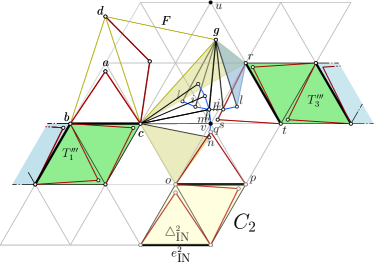
Suppose now that all $\triangle^{1}_{\textrm{IN}}$, $\triangle^{2}_{\textrm{IN}}$, and $\triangle^{3}_{\textrm{IN}}$ lie inside $\cal T$. We prove that the $(\alpha,\beta)$-clause gadget does not admit a feasible planar straight-line realization. We analyze the possible planar straight-line realizations of the flag gadget $F$. By Property 6 and statement (a) of Lemma 9, the triangle $(h,g,c)$ is drawn outside the triangle $(g,d,c)$. On the other hand, by statement (b) of Lemma 9, we have that either (i) the vertex $n$ lies outside the triangle $(h,g,c)$ (refer to LABEL:fig:clause_gadget_hexagon-a), (ii) the vertex $l$ lies outside the triangle $(h,g,c)$ (refer to LABEL:fig:clause_gadget_hexagon-b), or (iii) both vertices $n$ and $l$ lie outside the triangle $(h,g,c)$. We show next that in all cases, there is an intersection between the edges two triangles of the $(\alpha,\beta)$-clause gadget.

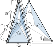
Consider first the case in which the vertex $n$ lies outside the triangle $(h,g,c)$; refer to LABEL:fig:clause_gadget_hexagon-a. The points $o,p,q$ are the vertices of the transmission triangle $\triangle_{\textrm{OUT}}$ of $C_{2}$. We prove that $\widehat{con}+\widehat{qop}>120^{\circ}$ and that the length of the segment $\overline{on}$ is smaller than $w_{2}$. These two statements imply that the segment $\overline{cn}$ intersects the segment $\overline{oq}$. To prove both statements we consider an auxiliary isosceles triangle with vertices $n$, $c$, $o$ (note that only the side $\overline{cn}$ of the triangle $(n,c,o)$ corresponds to an edge of $H_{\phi}$). We have that:

• The internal angle at $c$ is $\widehat{{nco}}\simeq 48.74^{\circ}$. Namely, $\widehat{nco}:=240^{\circ}-\widehat{bcd}-\widehat{dcg}-\widehat{gch}-2\lambda$. By Property 5, we obtain $\widehat{{nco}}\simeq 240^{\circ}-71.91^{\circ}-60^{\circ}-36.39^{\circ}-2\cdot 11.48^{\circ}=48.74^{\circ}$.

• The internal angle at $o$ is $\widehat{con}\simeq(180^{\circ}-\widehat{nco})/2=65.63^{\circ}$.

• The segments $\overline{co}$ and $\overline{cn}$ have length $w_{1}$.

• The segment $\overline{on}$ has length $2w_{1}\sin(\frac{\widehat{nco}}{2})\simeq 0.83$.

Since the triangle $(q,o,p)$ is a transmission triangle, we have that $\widehat{qop}=\arccos(\frac{w_{1}}{2w_{2}})=\arccos(\frac{1}{1.8})=56.25^{\circ}$, and the segment $\overline{oq}$ has length $w_{2}$. Hence, $\widehat{con}+\widehat{qop}\simeq 65.63^{\circ}+56.25^{\circ}=121.88^{\circ}>120^{\circ}$, and $|\overline{oq}|=w_{2}=0.9>|\overline{on}|\simeq 0.83$. This implies that $\overline{cn}$ intersects $\overline{oq}$, as claimed.

Consider now the case in which the vertex $l$ lies outside the triangle $(h,g,c)$; refer to LABEL:fig:clause_gadget_hexagon-b. The points $r,t,s$ denote the vertices of the transmission triangle $\triangle_{\textrm{OUT}}$ of $T^{\prime\prime\prime}_{3}$. Let $u$ be the point at distance $w_{1}=1$ from $r$ such that the ray from $r$ through $u$ has slope $120^{\circ}$. We show that $\widehat{gru}+\widehat{lrg}+\widehat{trs}>180^{\circ}$ and that the length of the segment $\overline{rl}$ is smaller than $w_{2}$. These two statements imply that the segment $\overline{gl}$ intersects the segment $\overline{rs}$. To prove both statements we consider two auxiliary isosceles triangles. The first triangle has vertices $c$, $g$, and $r$. We have that:

• The segment $\overline{cg}$ has length $w_{4}$.

• The segment $\overline{cr}$ has length $|\overline{cr}|=2\frac{\sqrt{3}}{2}=\sqrt{3}$.

• The internal angle at $c$ is $\widehat{gcr}\simeq 18.09^{\circ}$. Namely, $\widehat{bcr}=150^{\circ}$. Further, $\widehat{bcg}=\widehat{bcd}+\widehat{dcg}$ and, by Property 5, we have $\widehat{bcg}\simeq 71.91^{\circ}+60^{\circ}=131.91^{\circ}$, hence $\widehat{gcr}=\widehat{bcr}-\widehat{bcg}\simeq 18.09^{\circ}$.

• The segment $\overline{gr}$ has length $|\overline{gr}|\simeq 0.54$. Namely, by the law of cosines, we have $|\overline{gr}|^{2}=|\overline{cg}|^{2}+|\overline{cr}|^{2}-2|\overline{cg}|\cdot|\overline{cr}|\cdot\cos(\widehat{gcr})$. Since $|\overline{cg}|=w_{4}=1.61$ and $|\overline{cr}|=\sqrt{3}$, we obtain $|\overline{gr}|^{2}\simeq 2.5921+3-2\cdot 1.61\cdot\sqrt{3}\cdot\cos(18.09^{\circ})\simeq 0.29$, hence $|\overline{gr}|\simeq 0.54$.

• The internal angle at $r$ is $\widehat{crg}\simeq 68.25^{\circ}$. Namely, by the law of cosines, we have $\widehat{crg}=\arccos\left(\frac{|\overline{gr}|^{2}+|\overline{cr}|^{2}-|\overline{gc}|^{2}}{2|\overline{gr}|\cdot|\overline{cr}|}\right)\simeq\arccos\left(\frac{0.54^{2}+3-1.61^{2}}{2\cdot 0.54\cdot\sqrt{3}}\right)\simeq\arccos\left(\frac{0.6924}{1.8684}\right)\simeq\arccos(0.3706)\simeq 68.25^{\circ}$.

• The internal angle at $g$ is $\widehat{rgc}=180^{\circ}-\widehat{crg}-\widehat{gcr}\simeq 180^{\circ}-68.25^{\circ}-18.09^{\circ}=93.66^{\circ}$.

The second auxiliary triangle we consider has vertices $g$, $r$, and $l$. We have that:

• The segment $\overline{lg}$ has length $w_{1}=1$.

• The internal angle at $g$ is $\widehat{rgl}\simeq 34.31^{\circ}$. Namely, $\widehat{lgc}=\widehat{hgc}+2\lambda$. By Property 5, we have $\widehat{lgc}\simeq 36.39^{\circ}+2\cdot 11.48^{\circ}=59.35^{\circ}$. We obtain that $\widehat{rgl}=\widehat{rgc}-\widehat{lgc}\simeq 93.66^{\circ}-59.35^{\circ}=34.31^{\circ}$.

• The edge $\overline{lr}$ has length $|\overline{lr}|\simeq 0.63$. Namely, by the law of cosines, we have that $|\overline{lr}|^{2}=|\overline{lg}|^{2}+|\overline{rg}|^{2}-2|\overline{lg}|\cdot|\overline{rg}|\cos(\widehat{rgl})$, and hence $|\overline{lr}|\simeq\sqrt{1+0.54^{2}-2\cdot 0.54\cdot\cos(34.31^{\circ})}\simeq\sqrt{0.3995}\simeq 0.63$.

• The internal angle at $r$ is $\widehat{lrg}=117.2^{\circ}$. Namely, by the law of cosines, we have $\widehat{lrg}=\arccos\left(\frac{|\overline{gr}|^{2}+|\overline{lr}|^{2}-|\overline{gl}|^{2}}{2|\overline{gr}|\cdot|\overline{lr}|}\right)\simeq$ $\arccos\left(\frac{0.54^{2}+0.63^{2}-1^{2}}{2\cdot 0.54\cdot 0.63}\right)=\arccos\left(\frac{-0.3115}{0.6804}\right)\simeq\arccos(-0.4578)\simeq 117.2^{\circ}$.

Let $v$ be the point at distance $w_{1}=1$ from $r$ such that the ray from $r$ through $v$ has slope $240^{\circ}$. Note that $\widehat{vru}=\widehat{vrc}+\widehat{crg}+\widehat{gru}$, hence $\widehat{gru}=\widehat{vru}-\widehat{vrc}-\widehat{crg}\simeq 120^{\circ}-30^{\circ}-68.25^{\circ}=21.75^{\circ}$. On the other hand, since the triangle $(r,s,t)$ is a transmission triangle, we have $\widehat{trs}\simeq 56.25^{\circ}$ and the segment $\overline{rs}$ has length $w_{2}$. Hence $\widehat{gru}+\widehat{lrg}+\widehat{trs}\simeq 21.75^{\circ}+117.2^{\circ}+56.25^{\circ}=195.2^{\circ}>180^{\circ}$, and $|\overline{rl}|\simeq 0.63<w_{2}=0.9$. This implies that $\overline{gl}$ intersects $\overline{rs}$, as claimed, and concludes the proof of the lemma. ∎

4.4 Proof of the reduction

We are now ready to prove the main result of this section.

Proof of Theorem 4.1.

We first prove that, starting from the boolean formula $\phi$, the incidence graph $G_{\phi}$ of $\phi$, and the monotone rectilinear representation $\Gamma_{\phi}$ of $G_{\phi}$, we can construct the $2$-tree $H_{\phi}$ in polynomial time. The first step of the construction is to obtain from $\Gamma_{\phi}$ the auxiliary drawing $\Gamma^{*}_{\phi}$ we described in Section 4.1. By Lemma 4, we can construct $\Gamma^{*}_{\phi}$ in polynomial time. The next step is to construct $H_{\phi}$ using $\Gamma^{*}_{\phi}$ as an auxiliary tool. We obtain $H_{\phi}$ by introducing a variable gadget, a clause gadget, and a transmission gadget for each variable, clause, and edge in $G_{\phi}$, respectively, and then combining these gadgets together by identifying their attachment edges. In particular, we exploit $\Gamma^{*}_{\phi}$ to (i) define the size $k$ of each $k$-transmission gadget that represents an edge of $G_{\phi}$, (ii) define the parameters $\alpha$ and $\beta$ of each $(\alpha,\beta)$-clause gadget, and (iii) select the appropriate attachment edges to combine the gadgets together. We then merge the frames of the variable gadgets that are consecutive in the left-to-right order of the rectangles representing variables in $\Gamma^{*}_{\phi}$. This is done by means of ladder gadgets (the shaded blue triangles in Fig. 7), which are maximal outerpaths, each composed of a sequence of frame triangles. We have that $H_{\phi}$ is a $2$-tree by repeated applications of Lemma 5, and the union of the frame triangles induces a maximal outerplanar graph. Moreover, from the detailed description of the gadgets construction of Section 4.3, it is not hard to see that $H_{\phi}$ can be constructed in polynomial time.

We now prove that $H_{\phi}$ admits a planar straight-line realization if and only if $\phi$ is satisfiable. Suppose first that $H_{\phi}$ admits a planar straight-line realization $\Gamma_{H}$. We show that $\phi$ is satisfiable. For each variable $v$ of $\phi$, consider the variable gadget $\mathcal{V}$ of $H_{\phi}$ modeling $v$, the truth-assignment triangle $\triangle_{\textrm{IN}}$ of $\mathcal{V}$, and the frame triangle $\triangle_{s}$ of the split gadget $S_{\delta_{\phi}}$ of $\mathcal{V}$; refer to Figs. 10 and 11. We set $v=\texttt{True}$ if and only if $\triangle_{\textrm{IN}}$ is drawn inside $\triangle_{s}$. We next prove this truth assignment satisfies every clause $c$ of $\phi$. Assume that $c$ is a positive clause with variables $v_{1}$, $v_{2}$, and $v_{3}$, that is, $c=(v_{1}\vee v_{2}\vee v_{3})$. The proof for the case in which $c$ is negative is symmetric. Let $\mathcal{C}$ denote the clause gadget modeling $c$ and, for $i=1,2,3$, let $\mathcal{T}_{i}$ denote the transmission gadget modeling the edge $(v_{i},c)$ of $G_{\phi}$. From the construction of the clause gadget, the realization of $\mathcal{C}$ in $\Gamma_{H}$ is such that the frame of the components of $\mathcal{C}$ are bounded by a trapezoid $\mathcal{T}$. By Lemma 10, at least one of the triangles $\triangle^{1}_{\textrm{IN}}$, $\triangle^{2}_{\textrm{IN}}$, and $\triangle^{3}_{\textrm{IN}}$ of $\mathcal{C}$ lies outside $\mathcal{T}$. We assume w.l.o.g. that it is actually $\triangle^{1}_{\textrm{IN}}$ the triangle that lies outside $\mathcal{T}$. Then $\triangle^{1}_{\textrm{IN}}$ lies inside the frame triangle $\triangle_{t}$ of the transmission gadget $\mathcal{T}_{1}$. Let $\mathcal{V}_{1}$ denote the variable gadget modeling the variable $v_{1}$. By Lemma 6, there exists an index $j\in\{1,2,\dots,\delta_{\phi}\}$ such that the transmission triangle $\triangle^{j}_{\textrm{OUT}}$ of $\mathcal{V}_{1}$ lies inside the frame triangle $\triangle^{j}_{t}$ of $\mathcal{V}_{1}$ (for such index $j$ the transmission triangle $\triangle^{j}_{\textrm{OUT}}$ is shared by $\mathcal{V}_{1}$ and $\mathcal{T}_{1}$). Thus, by Lemma 8, the truth-assignment triangle $\triangle_{\textrm{IN}}$ of $\mathcal{V}_{1}$ is drawn inside the frame triangle $\triangle_{s}$ of the split gadget $S_{\delta_{\phi}}$ of $\mathcal{V}_{1}$. This implies in turn that $v_{1}$ is assigned the value True. Since this variable appears as a positive literal in $c$, we have that $c$ is satisfied. This shows that the constructed truth assignment satisfies all the clauses of $\phi$.

Suppose now that $\phi$ is satisfiable. We show that $H_{\phi}$ admits a planar straight-line realization $\Gamma_{H}$. Let $\tau$ be a satisfying truth assignment for $\phi$. For each variable $v$ of $\phi$, let $\tau(v)$ denote the truth value of $v$ in $\tau$. Observe that, up to a rigid transformation, the union of all the frame triangles of $H_{\phi}$ admits a unique planar straight-line realization. We initialize $\Gamma_{H}$ to such a realization. Further, for each variable $v$, we adopt the configuration of LABEL:fig:variable-b if $\tau(v)=\texttt{True}$ and the configuration of LABEL:fig:variable-c if $\tau(v)=\texttt{False}$. For each transmission gadget modeling an edge of $G_{\phi}$ incident to a variable $v$ and to a positive clause $c$, we adopt the configuration of LABEL:fig:transmission_gadget-a(right) if $\tau(v)=\texttt{True}$ and the configuration of LABEL:fig:transmission_gadget-a(left) if $\tau(v)=\texttt{False}$; a symmetric choice is made if $c$ is negative. Since, for each clause $c$ of $\phi$, there exists at least one literal that is True, the triangle $\triangle^{i}_{\textrm{IN}}$, $i\in\{1,2,3\}$, associated with this literal is drawn outside the trapezoid $\cal T$ that bounds the frame of the components of $\mathcal{C}$ in $\Gamma_{H}$. Then, by Lemma 10, the clause gadget modeling $c$ admits a feasible planar straight-line realization; such realizations are used to complete the planar straight-line realization $\Gamma_{H}$ of $H_{\phi}$. This concludes the proof of Theorem 4.1.

5 A Linear-time Algorithm for 2-trees with Two Edge Lengths

In this section, we study the FEPR problem for weighted $2$-trees in which each edge can only have one of at most two distinct lengths. We prove that, in this case, the FEPR problem is linear-time solvable. We first solve the case in which all the edges are prescribed to have the same length; we remark that the FEPR problem is NP-hard for general weighted planar graphs in which all the edges have the same length [28].

Theorem 5.1.

Let $G=(V,E,\lambda)$ be an $n$-vertex weighted $2$-tree, where $\lambda:E\rightarrow\{w\}$ with $w\in\mathbb{R}^{+}$. There exists an $O(n)$-time algorithm that tests whether $G$ admits a planar straight-line realization and, in the positive case, constructs such a realization.

Proof.

Suppose that there exists a planar straight-line realization $\Gamma$ of $G$. Since all the edges of $G$ have length $w$, every $3$-cycle of $G$ is represented in $\Gamma$ by an equilateral triangle of side $w$, hence no triangle can be contained inside any other triangle in $\Gamma$. This, together with the fact that $G$ is a $2$-tree, implies that $\Gamma$ is an outerplanar drawing of $G$. Thus, if $G$ admits a planar straight-line realization, then it is a maximal outerplanar graph and, as such, it has a unique outerplane embedding [39, 47].

Therefore, in order to test whether $G$ has a planar straight-line realization, we test whether it is an outerplanar graph; this can be done in $O(n)$ time [21, 38, 50]. If the test fails, we conclude that $G$ admits no planar straight-line realization. Otherwise, we construct in $O(n)$ time its unique outerplane embedding [21, 38, 39, 47, 50]. Finally, by means of Theorem 3.1, we test in $O(n)$ time whether $G$ has a planar straight-line realization that respects the computed outerplane embedding. If the test fails, we conclude that $G$ admits no planar straight-line realization. Otherwise, Theorem 3.1 provides us with the desired planar straight-line realization of $G$. ∎

We now extend our study to weighted graphs in which each is assigned with one of two possible lengths. We have the following main theorem.

Theorem 5.2.

Let $G=(V,E,\lambda)$ be an $n$-vertex weighted $2$-tree, where $\lambda:E\rightarrow\{w_{1},w_{2}\}$ with $w_{1},w_{2}\in\mathbb{R}^{+}$. There exists an $O(n)$-time algorithm that tests whether $G$ admits a planar straight-line realization and, in the positive case, constructs such a realization.

In the remainder of the section, we prove Theorem 5.2. Hereafter, we assume, w.l.o.g., that $w_{1}<w_{2}$. Note that the realization of any $3$-cycle of $G$ is one of the following types of triangles (refer to Fig. 16):

1. an equilateral triangle of side $w_{1}$ (a small equilateral triangle),

2. an equilateral triangle of side $w_{2}$ (a big equilateral triangle),

3. an isosceles triangle with base $w_{1}$ and two sides of length $w_{2}$ (a tall isosceles triangle), and

4. an isosceles triangle with base $w_{2}$ and two sides of length $w_{1}$ (a flat isosceles triangle).

Any triangle of one of the types above is called an interesting triangle.

Figure 16: The four interesting triangles. Since $w_{1}<w_{2}$, the angles in gray are always less than $60^{\circ}$, while the angles in white are always greater than $60^{\circ}$.

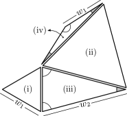
While small equilateral, big equilateral and tall isosceles triangle exist regardless of the values of $w_{1}$ and $w_{2}$, flat isosceles triangles do not exist under the condition described in the following property.

Property 9.

If $w_{2}\geq 2w_{1}$, then no $3$-cycle of $G$ is realized as a flat isosceles triangle.

Proof.

By assumption, every $3$-cycle of $G$ satisfies the triangle inequality, that is, the sum of the lengths prescribed to any two edges is larger than the length of the third edge. Hence, if $w_{2}\geq 2w_{1}$, then no $3$-cycle of $G$ can have two edges with length $w_{1}$ and the third edge with length $w_{2}$. ∎

5.1 Containment among triangles

The first central ingredient of our algorithm are the conditions satisfied by interesting triangles when they are drawn inside each other in a planar straight-line realization of $G$. In the following, we denote with $r$ the ratio $\frac{w_{2}}{w_{1}}>1$. Regardless of the value of $r$, the following lemma holds true.

Lemma 11.

The interesting triangles satisfy the two properties below.

1. No interesting triangle can be drawn inside a small equilateral or a flat isosceles triangle.

2. Neither a big equilateral nor a tall isosceles triangle can be drawn inside any interesting triangle.

Proof.

Let $\triangle_{1}$ and $\triangle_{2}$ be any two interesting triangles. We make a case by case analysis based on the types of interesting triangles of $\triangle_{1}$ and $\triangle_{2}$. In both statment (a) and (b) we have the following common case: If $\triangle_{1}$ is the same type of interesting triangle as $\triangle_{2}$, then $\triangle_{1}$ and $\triangle_{2}$ are congruent, hence neither triangle can be drawn inside the other.

We now prove statement (a). We suppose that $\triangle_{2}$ is either small equilateral or flat isosceles, and show that $\triangle_{1}$ cannot be drawn inside $\triangle_{2}$ regardless of the type of $\triangle_{1}$. We have the following cases:

• $\triangle_{2}$ is small equilateral and $\triangle_{1}$ is either big equilateral, tall isosceles, or flat isosceles.

  In this case $\triangle_{1}$ cannot be drawn inside $\triangle_{2}$ by Theorem 2.1.

• $\triangle_{2}$ is flat isosceles.

  • $\triangle_{1}$ is big equilateral.

    If $\triangle_{1}$ and $\triangle_{2}$ do not share any edge, then $\triangle_{1}$ cannot be drawn inside $\triangle_{2}$ by Theorem 2.1. If instead $\triangle_{1}$ and $\triangle_{2}$ share an edge, then $\triangle_{1}$ cannot be drawn inside $\triangle_{2}$ by Property c of Lemma 1.

  • $\triangle_{1}$ is tall isosceles.

    If $\triangle_{1}$ and $\triangle_{2}$ do not share any edge, then $\triangle_{1}$ cannot be drawn inside $\triangle_{2}$ by Theorem 2.1. If instead $\triangle_{1}$ and $\triangle_{2}$ share an edge, then $\triangle_{1}$ cannot be drawn inside $\triangle_{2}$ by Property a of Lemma 1.

  • $\triangle_{1}$ is small equilateral.

    If $\triangle_{1}$ and $\triangle_{2}$ share an edge, then $\triangle_{1}$ cannot be drawn inside $\triangle_{2}$ by Property c of Lemma 1. Consider instead that $\triangle_{1}$ does not share an edge with $\triangle_{2}$. Let $a,b,c$ be the vertices of $\triangle_{2}$, where $\overline{bc}$ is the side of $\triangle_{2}$ with length $w_{2}$; refer to Fig. 17. Let $d$ be the orthogonal projection of the vertex $a$ on the segment $\overline{bc}$, let $R_{1}$ denote the closed region bounded by the triangle with vertices $a,c,d$, and let $R_{2}$ denote the closed region bounded by the triangle with vertices $a,b,d$. Since $\triangle_{2}$ is flat isosceles, by Property 9 we have $w_{2}<2w_{1}$, hence the lengths of the segments $\overline{bd}$, $\overline{cd}$, and $\overline{ad}$ are all smaller than $w_{1}$. This implies that the only pair of points inside $R_{1}$ (resp. inside $R_{2}$) at distance greater than or equal to $w_{1}$ is $(a,c)$ (resp. $(a,b)$). Suppose, for a contradiction, that $\triangle_{1}$ is contained inside $\triangle_{2}$. Then two vertices of $\triangle_{1}$ are contained in the same triangle $R_{i}$, say they are contained in $R_{1}$. Since at least one of such two vertices does not coincide with $a$ or $c$ (otherwise $\triangle_{1}$ and $\triangle_{2}$ would share an edge), the distance between such two vertices is smaller than $w_{1}$, while the length of the edge between them is at least $w_{1}$, a contradiction.

Figure 17: Illustration for the proof of statement (a) of Lemma 11.

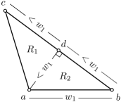
We now prove statement (b). We suppose that $\triangle_{1}$ is either big equilateral or tall isosceles, and prove that $\triangle_{1}$ cannot be drawn inside $\triangle_{2}$ regardless of the type of $\triangle_{2}$. Note that, if $\triangle_{2}$ is small equilateral or flat isosceles, then $\triangle_{1}$ cannot be drawn inside $\triangle_{2}$ by statement (a) of the present lemma. We can hence assume that $\triangle_{2}$ is either a big equilateral triangle or a tall isosceles triangle. We have the following cases.

• $\triangle_{1}$ and $\triangle_{2}$ are of different types of interesting triangles and do not share any edge.

  In this case $\triangle_{1}$ cannot be drawn inside $\triangle_{2}$ by Theorem 2.1.

• $\triangle_{1}$ is tall isosceles, $\triangle_{2}$ is big equilateral, and $\triangle_{1}$ and $\triangle_{2}$ share an edge.

  In this case $\triangle_{1}$ cannot be drawn inside $\triangle_{2}$ by Property b of Lemma 1.

• $\triangle_{1}$ is big equilateral, $\triangle_{2}$ is tall isosceles, and $\triangle_{1}$ and $\triangle_{2}$ share an edge.

  In this case $\triangle_{1}$ cannot be drawn inside $\triangle_{2}$ by Theorem 2.2.

This concludes the proof of the lemma. ∎

Let $T$ denote the decomposition tree of $G$. Suppose that a planar straight-line realization $\Gamma$ of $G$ exists. The second central ingredient of our algorithm is the next lemma.

Lemma 12.

Let $\triangle_{1}$ and $\triangle_{2}$ be two triangles realizing two different $3$-cycles of $G$ in $\Gamma$. Suppose that $\triangle_{1}$ is drawn inside $\triangle_{2}$. Then $\triangle_{1}$ is a leaf triangle of $T$ that shares a side with $\triangle_{2}$.

Proof.

By statement (a) of Lemma 11, we have that $\triangle_{2}$ is either big equilateral or tall isosceles. We discuss the two cases separately.

Suppose first that $\triangle_{2}$ is big equilateral. Consider any interesting triangle $\triangle_{3}$ that is drawn inside $\triangle_{2}$ in $\Gamma$ and shares a side with $\triangle_{2}$. Note that $\triangle_{3}$ is flat isosceles; namely, $\triangle_{3}$ cannot be tall isosceles or big equilateral by statement (a) of Lemma 11, and it cannot be small equilateral since the sides of $\triangle_{2}$ have length $w_{2}$. Now suppose, for the sake of contradiction, that an interesting triangle $\triangle_{4}$ shares a side of length $w_{1}$ with $\triangle_{3}$. Let $v$ be the common vertex between $\triangle_{2}$, $\triangle_{3}$, and $\triangle_{4}$. If $\triangle_{4}$ is small equilateral or tall isosceles, as in Fig. 18(a) with $v=a$, then the sum of the angles at $v$ of $\triangle_{3}$ and $\triangle_{4}$ exceeds $60^{\circ}$. Hence $\triangle_{4}$ crosses $\triangle_{2}$, a contradiction. Further, if $\triangle_{4}$ is flat isosceles, as in Fig. 18(a) with $v=b$, then $\triangle_{4}$ crosses $\triangle_{2}$ by Theorem 2.1. It follows that the only interesting triangles inside $\triangle_{2}$ are flat isosceles triangles that are leaves of $T$ and that share a side with $\triangle_{2}$.

Suppose next that $\triangle_{2}$ is tall isosceles. The proof follows similar arguments as for the case in which $\triangle_{2}$ is big equilateral, although, in this case, we distinguish two subcases. Namely, an interesting triangle $\triangle_{3}$ that is drawn inside $\triangle_{2}$ and that shares a side with $\triangle_{2}$ can be either small equilateral (and then it shares a side of length $w_{1}$ with $\triangle_{2}$) as in Fig. 18(b), or flat isosceles (and then it shares a side of length $w_{2}$ with $\triangle_{2}$) as in Fig. 19(a).

(a)

(b)

Figure 18: Two illustrations for the proof of Lemma 12. (18(a)) The case in which $\triangle_{2}$ is a big equilateral triangle and $\triangle_{3}$ is a flat isosceles triangle. (18(b)) The case in which $\triangle_{2}$ is a tall isosceles triangle and $\triangle_{3}$ is a small equilateral triangle. In both figures, the possible cases for $\triangle_{4}$ are shown with dashed lines.

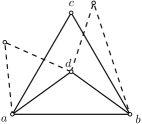
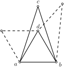
Consider first the subcase in which $\triangle_{3}$ is small equilateral. Suppose, for the sake of contradiction, that an interesting triangle $\triangle_{4}$ shares a side of length $w_{1}$ with $\triangle_{3}$. Let $v$ be the common vertex between $\triangle_{2}$, $\triangle_{3}$, and $\triangle_{4}$. If $\triangle_{4}$ is small equilateral or tall isosceles, as in Fig. 18(b) with $v=a$, then the sum of the angles at $v$ of $\triangle_{3}$ and $\triangle_{4}$ exceeds $90^{\circ}$. Hence $\triangle_{4}$ crosses $\triangle_{2}$, a contradiction. On the other hand, if $\triangle_{4}$ is flat isosceles, as in Fig. 18(b) with $v=b$, then $\triangle_{4}$ crosses $\triangle_{2}$ by Theorem 2.1.

Consider next the subcase in which $\triangle_{3}$ is flat isosceles. Suppose, for the sake of contradiction, that an interesting triangle $\triangle_{4}$ shares a side of length $w_{1}$ with $\triangle_{3}$. Let $v$ be the common vertex between $\triangle_{2}$, $\triangle_{3}$, and $\triangle_{4}$. Let $a$ and $b$ be the vertices incident to the base of $\triangle_{2}$, and let $c$ be the third vertex of $\triangle_{2}$; refer to Fig. 19(a). The following cases arise depending of whether $v$ is equal to $c$ or $a$:

• Case 1: $v=c$. If $\triangle_{4}$ is small equilateral or tall isosceles, then the angle at $v$ of $\triangle_{4}$ is larger than or equal to $60^{\circ}$, which is larger than the angle at $v$ of $\triangle_{2}$. Hence $\triangle_{4}$ crosses $\triangle_{2}$. If $\triangle_{4}$ is instead flat isosceles, then $\triangle_{4}$ crosses $\triangle_{2}$ by Theorem 2.1. In both case we have a contradiction.

• 

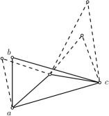
  (a)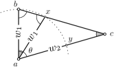

  

  (b)

  Figure 19: Two illustrations for the proof of Lemma 12, for the case in which $\triangle_{2}$ is a tall isosceles triangle and $\triangle_{3}$ is a flat isosceles triangle. (19(a)) The case in which $v=c$ and $\triangle_{4}$ (in dashed lines) is flat isosceles or tall isosceles, and the case in which $v=a$ and $\triangle_{4}$ (in dashed lines) is small equilateral. (19(b)) A focus on the case in which $v=a$ and $\triangle_{4}$ is small equilateral.

  Case 2: $v=a$. If $\triangle_{4}$ is flat isosceles or tall isosceles, then $\triangle_{4}$ crosses $\triangle_{2}$ by Theorem 2.1, a contradiction. Consider that $\triangle_{4}$ is instead small equilateral, as in Fig. 19(a). Let $\angle z$ denote the interior angle of $\triangle_{2}$ at vertex $z$, for $z\in\{a,b,c\}$. Let $C$ be the circle with center on $a$ and radius $w_{1}$. The circle cuts the interior of the segment $\overline{ac}$ in a point $y$ and it cuts the interior of the segment $\overline{bc}$ in a point $x$, since the length of $\overline{ac}$ is $w_{2}>w_{1}$ and since $\angle b<90^{\circ}$; see Fig. 19(b). If $\triangle_{4}$ is drawn inside $\triangle_{2}$, the vertices of $\triangle_{4}$ that are different from $a$ lie on the circular arc of $C$ that connects $x$ and $y$ through the interior of $\triangle_{2}$. Furthermore, since $\triangle_{4}$ is equilateral, the internal angle at $a$ of the triangle with vertices $a,c,x$ should be greater than $60^{\circ}$. Let $\theta$ denote such angle. We show that $\theta$ is actually less than $60^{\circ}$, which is a contradiction. Note that $\triangle_{2}$ and the triangle with vertices $a,b,x$ are similar to each other, hence $\theta=\angle a-\angle c$. Since $\angle c+2\angle a=180^{\circ}$ we have that

  $$\theta=3\angle a-180^{\circ}.$$ (1)

  On the other hand, we have that $\cos(\angle a)=\frac{1}{2}\frac{w_{1}}{w_{2}}$ and, since $\triangle_{1}$ exists only if $\frac{w_{1}}{w_{2}}>\frac{1}{2}$, then $\cos(\angle a)>\frac{1}{4}$. Hence

  $$\angle a<\arccos(\frac{1}{4})\simeq 75.52^{\circ},$$ (2)

  and from Eqs. 1 and 2 we obtain that $\theta=3\angle a-180^{\circ}\simeq 46.56^{\text{o}}<60^{\text{o}}$.

It follows that the only triangles inside $\triangle_{2}$ are flat isosceles triangles and small equilateral triangles that are leaves of $T$ and that share a side with $\triangle_{2}$.

This concludes the proof of the lemma. ∎

5.2 Conflicts between leaf triangles

Hereafter, we assume that the decomposition tree $T$ of $G$ is rooted at any $3$-cycle whose sum of the edge lengths is maximum. Hence, the triangle realizing such a $3$-cycle cannot be drawn inside any other triangle in a planar straight-line realization of $G$.

The framework of $G$ is the subgraph $G_{F}\subseteq G$ obtained as follows: For each leaf triangle $\triangle_{i}$ that can be drawn inside a triangle $\triangle_{j}$, which is either its parent or one of its siblings, we remove from $G$ the vertex $v$ that $\triangle_{i}$ does not share with $\triangle_{j}$, along with the two edges incident to $v$. Note that $G_{F}$ is a $2$-tree. Further, by Lemma 12, in any planar straight-line realization $\Gamma$ of $G$, the triangles we removed from $G$ in order to define $G_{F}$ are the only triangles that can be drawn inside other triangles representing $3$-cycles of $G$. It follows that the restriction of $\Gamma$ to $G_{F}$ is an outerplanar drawing. Hence, we start by testing if $G_{F}$ is outerplanar, which can be done in linear time [21, 38, 50]; in the negative case, we reject the instance. In the positive case, we test whether $G_{F}$ admits a planar straight-line realization respecting its unique outerplane embedding $\cal E$. Both the computation of $\cal E$ and the test can be performed in linear time using the algorithms in [21, 38, 50] and Theorem 3.1, respectively. If the test is negative we reject the instance, otherwise we have a planar straight-line realization $\Gamma_{F}$ of $G_{F}$ with embedding $\cal E$.

Let $L_{\triangle}$ denote the set of triangles that were removed from $G$ to obtain $G_{F}$. The third central ingredient of our algorithm is a characterization of the conditions under which $\Gamma_{F}$ can be extended to a planar straight-line realization of $G$, by drawing in $\Gamma_{F}$ all the triangles of $L_{\triangle}$.

Let $\triangle=(a,b,c)$ be a triangle of $L_{\triangle}$ such that $e=(a,b)$ is the unique edge shared by $\triangle$ and $G_{F}$. Suppose we want to add a drawing of $\triangle$ to $\Gamma_{F}$. If $e$ is incident to two internal faces of $\Gamma_{F}$, then we call internal embedding to each of the two possible drawings of $\triangle$, regardless of whether $a,b,c$ appear in clockwise or counter-clockwise order when traversing $\triangle$. Consider that $e$ is instead incident to one internal face and to the outer face of $\Gamma_{F}$. Suppose that $a$ precedes $b$ in a counter-clockwise traversal of the outer face of $\Gamma_{F}$. If $\triangle$ is drawn such that $a,b,c$ appear in clockwise order when traversing $\triangle$, then we call such drawing of $\triangle$ an outer embedding. Otherwise, we call such drawing of $\triangle$ an internal embedding.

Consider a straight-line realization $\Gamma$ of $G$ that extends $\Gamma_{F}$; that is, whose restriction to $G_{F}$ is $\Gamma_{F}$. Suppose that $\Gamma$ is not planar. We now classify the possible crossings involving triangles in $L_{\triangle}$.

First, suppose there is a triangle $\triangle\in L_{\triangle}$ whose drawing in $\Gamma$ crosses an edge of $\Gamma_{F}$. If the drawing of $\triangle$ is an outer embedding, then we say it induces a framework conflict. If the drawing of $\triangle$ is instead an internal embedding, then we say it induces an overlapping conflict. Second, consider two triangles $\triangle_{i}$ and $\triangle_{j}$ of $L_{\triangle}$. If the drawings of $\triangle_{i}$ and $\triangle_{j}$ in $\Gamma$ are both outer embeddings, neither of them induces a framework conflict, and they cross each other, then we say that such drawings induce an external conflict. Similarly, if the drawings of $\triangle_{i}$ and $\triangle_{j}$ in $\Gamma$ are both internal embeddings, neither of them induces an overlapping conflict, and they cross each other, then we say that such drawings induce an internal conflict. In both cases, we say that the drawings of $\triangle_{i}$ and $\triangle_{j}$ conflict with each other.

We have the following.

Lemma 13.

Let $\triangle_{i}$ and $\triangle_{j}$ be two triangles in $L_{\triangle}$, and $\Gamma$ be a straight-line realization of $G$ that extends $\Gamma_{F}$. Suppose that there exists a triangle $\triangle\in\Gamma_{F}$ such that both $\triangle_{i}$ and $\triangle_{j}$ are drawn inside $\triangle$ in $\Gamma$. The drawings of $\triangle_{i}$ and $\triangle_{j}$ induce an internal conflict if at least one of the following statements is true:

1. $\triangle_{i}$ and $\triangle_{j}$ share an edge.

2. $\sqrt{3}<r\leq 2\cos(15^{\circ})\simeq 1.93$ and $\triangle$ is a tall isosceles triangle.

3. $1<r\leq\sqrt{3}$.

Proof.

By statement (a) of Lemma 11 and since each of $\triangle_{i}$ and $\triangle_{j}$ is drawn inside $\triangle$, the triangle $\triangle$ is either tall isosceles or big equilateral. Furthermore, by statement (b) of Lemma 11, each of $\triangle_{i}$ and $\triangle_{j}$ is either small equilateral or flat isosceles. By Lemma 12, the triangles $\triangle_{i}$ and $\triangle$ share an edge and so do $\triangle_{j}$ and $\triangle$.

Consider first the case in which $\triangle_{i}$ shares an edge with $\triangle_{j}$, as described in statement (a). Note that, since $G$ is a $2$-tree, the triangles $\triangle_{i}$, $\triangle_{j}$, and $\triangle$ actually share the same edge. By statement (a) of Lemma 11, $\triangle_{i}$ and $\triangle_{j}$ cannot be drawn inside each other regardless of their types. Since $\triangle_{i}$ and $\triangle_{j}$ are drawn inside the same triangle and they cannot be drawn inside each other, their drawings induce an internal conflict inside $\triangle$. This proves statement (a).

Consider now the case in which $\triangle_{i}$ and $\triangle_{j}$ do not share an edge. The triangles $\triangle_{i}$ and $\triangle_{j}$ induce an internal conflict inside $\triangle$ depending on the types of $\triangle_{i}$, $\triangle_{j}$, $\triangle$, and the value of $r$. Note that $r$ is necessarily less than $2$ since, otherwise, by Property 9 both $\triangle_{i}$ and $\triangle_{j}$ would be small equilateral triangles and they could not share each a different side of $\triangle$, since $\triangle$ has at most one side of length $w_{1}$. By a simple geometric argument we can deduce that two triangles are drawn inside $\triangle$ without inducing internal conflicts in the following cases (refer to Fig. 20):

1. If $2\cos(15^{\circ})\simeq 1.93<r<2$ and $\triangle$ is tall isosceles, then two flat isosceles triangles and one small equilateral triangle can be drawn inside $\triangle$ without inducing internal conflicts.

2. If $\sqrt{3}\simeq 1.73<r<2$ and $\triangle$ is big equilateral, then three flat isosceles can be drawn inside $\triangle$ without inducing internal conflicts.

The limit values $r=2\cos(15^{\circ})$ and $r=\sqrt{3}$ split the interval $1<r<2$ into the following three intervals. First, if $2\cos(15^{\circ})<r<2$, then the cases (i) and (ii) are both possible. Hence, $\triangle_{i}$ and $\triangle_{j}$ can be drawn inside $\triangle$ without inducing internal conflicts, regardless of their types. Second, if $\sqrt{3}<r\leq 2\cos(15^{\circ})$ then the case (i) is no longer possible. Hence, as described in statement (b), $\triangle_{i}$ and $\triangle_{j}$ induce an internal conflict inside $\triangle$ if $\triangle$ is a tall isosceles triangle. Finally, if $1<r\leq\sqrt{3}$, then none of the cases is possible. Hence, as described in statement (c), $\triangle_{i}$ and $\triangle_{j}$ induce an internal conflict inside $\triangle$ regardless of their types. ∎

Figure 20: Illustration for the proof of Lemma 13. The vertices that $\triangle_{i}$ and $\triangle_{j}$ do not share with $\triangle$ lie on the circumcenter of $\triangle$. On the left, the case in which $\triangle$ is tall isosceles (the segments between the circumcenter of $\triangle$ and its vertices all have the same length $l$). On the right, the case in which $\triangle$ is big equilateral.

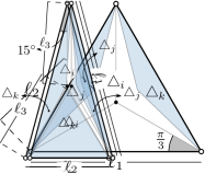
From Lemma 13 we obtain the following necessary condition for the existence of a planar straight-line realization of $G$ extending $\Gamma_{F}$.

Lemma 14.

If there exists a planar straight-line realization of $G$, then no subset of three triangles of $L_{\triangle}$ share a side.

Proof.

Suppose, for a contradiction, that there exists a planar straight-line realization $\Gamma$ of $G$ and that three triangles of $L_{\triangle}$ share an edge $e$. Consider two of such triangles that are on the same side of $e$ in $\Gamma$ and denote them by $\triangle_{i}$ and $\triangle_{j}$. If $\triangle_{i}$ and $\triangle_{j}$ do not cross each other in $\Gamma$, then they are contained one inside the other. However, this is not possible by statement (a) of Lemma 11. ∎

If $L_{\triangle}$ satisfies the condition stated in Lemma 14, we say that $L_{\triangle}$ is consistent.

Lemma 15.

If $L_{\triangle}$ is consistent, then there are $O(1)$ pairs of triangles of $L_{\triangle}$ whose drawings induce an internal conflict inside a triangle $\triangle\in\Gamma_{F}$.

Proof.

By Lemma 12, all the triangles of $L_{\triangle}$ that can be drawn inside $\triangle$ (including those inducing an internal conflict) share an edge with $\triangle$. By Lemma 14 and the assumed consistency of $L_{\triangle}$, there are at most $6$ of such triangles. Hence, the drawings of at most $\binom{6}{2}=15$ pairs of triangles can induce an internal conflict inside $\triangle$. ∎

5.3 The algorithm

We are now ready to describe the algorithm to solve the FEPR problem in $O(n)$ time when the edges of $G$ can only have one of two lengths. The algorithm consists of two stages. In the first stage, we compute the framework $G_{F}$ of $G$, and test whether $G_{F}$ admits a planar straight-line realization $\Gamma_{F}$. Such a realization is constructed in the positive case, and the input instance is rejected otherwise. In the second stage, we test whether $\Gamma_{F}$ can be extended to a planar straight-line realization $\Gamma$ of $G$, by drawing the triangles of $L_{\triangle}$ without inducing conflicts. In the positive case, we construct and report $\Gamma$ as the desired realization of $G$. As before, the input instance is rejected in the negative case. We describe the algorithm in detail next.

5.3.1 Computing a planar straight-line realization $\Gamma_{F}$ of the framework of $G$.

The first stage of the algorithm is formed by the following three steps.

Step A. Computing the framework $G_{F}$ of $G$ and the set $L_{\triangle}$ of leaf triangles.

To compute the framework of $G$ we first choose, among all the triangles of $G$, a triangle $\triangle_{O}$ with maximum sum of the length of its sides. Note that $\triangle_{O}$ cannot be drawn inside any other triangle of $G$, hence it does not belong to $L_{\triangle}$. We then compute the decomposition tree $T$ of $G$ rooted at $\triangle_{O}$. Note that, if $G$ admits a planar straight-line realization, then the degree of $T$ is bounded by a constant. Indeed, each edge of $G$ can be incident to at most two interesting triangles of the same type (and hence each $3$-cycle of $G$ can be adjacent to at most $24$ distinct $3$-cycles). We test whether the degree of $T$ is bounded by $24$ in $O(n)$ time. We reject the instance in the negative case. In the positive case we traverse $T$ looking for leaf triangles that can be drawn inside their parent or sibling triangles. By Lemma 12, these are the only triangles in $G$ that can be drawn inside any other triangle. We identify such triangles by means of Theorem 2.2. Since the degree of $T$ is in $O(1)$, each triangle has a constant number of sibling triangles, hence we can compute both $G_{F}$ and $L_{\triangle}$ in $O(n)$ time.

Step B. Testing if $L_{\triangle}$ is consistent.

The next step is to test if $L_{\triangle}$ is consistent. By Lemma 14, this is a necessary condition for the existence of a planar straight-line realization of $G$. This condition can be trivially tested in $O(n)$ time by looking at the triangles of $L_{\triangle}$ sharing an edge with a parent or a sibling triangle in $T$. The input instance is rejected in the negative case.

Step C. Constructing a planar straight-line realization $\Gamma_{F}$ of $G_{F}$.

The final step of this stage is to compute a planar straight-line realization of $G_{F}$, if it exists. We first test whether $G_{F}$ is outerplanar. If this is not the case we reject the instance. Otherwise, we construct its unique outerplane embedding in $O(n)$ time [21, 38, 50]. Then, by means of Theorem 3.4 we test in $O(n)$ time if $G_{F}$ admits a planar straight-line realization with the computed embedding. We construct $\Gamma_{F}$ in the positive case, and reject the input instance otherwise.

5.3.2 Extending $\Gamma_{F}$ to a planar straight-line realization of $G$.

In the second stage the algorithm distinguishes two cases, namely, the one in which $r\geq 2$ and the one in which $r<2$. In the former case, the algorithm is completed by means of a single step, called D.1, while in the latter case the algorithm is completed by means of four steps, called D.2, E, F, and G.

Case $\mathbf{r}\geq 2$. Note that, by Property 9, in this case there are no flat isosceles triangles. Hence, every leaf triangle $\triangle$ in $L_{\triangle}$ is a small equilateral triangle such that the parent or a sibling of $\triangle$ is a tall isosceles triangle. We act as described in the following step.

Step D.1.

Consider each edge $e$ of $G_{F}$ incident to a triangle in $L_{\triangle}$. If $e$ is incident to two triangles in $L_{\triangle}$, we draw them in $\Gamma_{F}$ on opposite sides of $e$. If $e$ is incident to one triangle $\triangle\in L_{\triangle}$, then we draw $\triangle$ inside any tall isosceles triangle incident to $e$ (recall that such a tall isosceles triangle is the parent or a sibling of $\triangle$). At the end of this process we obtain a straight-line realization $\Gamma$ of $G$, and a plane embedding $\mathcal{E}$ of $G$.

Lemma 16.

$G$ admits a planar straight-line realization if and only if $\Gamma$ is planar.

Proof.

Obviously, if $\Gamma$ is planar, then it is a planar straight-line realization of $G$.

We prove that, if $G$ admits a planar straight-line realization, then $\Gamma$ is planar. Consider an edge $e\in G_{F}$. Since $L_{\triangle}$ is consistent, the edge $e$ is shared by a set $L^{e}_{\triangle}\subseteq L_{\triangle}$ of at most two leaf triangles. Suppose that $e$ is an internal edge of $\Gamma_{F}$. Then, in $\Gamma$, each small equilateral triangle $L^{e}_{\triangle}$ is drawn as an internal embedding inside a tall isosceles triangle $\triangle^{*}\in G_{F}$. Note that no other triangle is drawn inside $\triangle^{*}$, since a tall isosceles triangle has a single side of length $w_{1}$. Hence, no triangle of $L^{e}_{\triangle}$ creates a crossing in $\Gamma$.

Suppose now that $e$ is incident to the outer face of $\Gamma_{F}$. If $L^{e}_{\triangle}$ consists of a single triangle, then the triangle is drawn as an internal embedding and, as above, it does not create crossings in $\Gamma$. If $L^{e}_{\triangle}$ consists instead of two triangles, then least one of them, say $\triangle_{s}$, is drawn as an outer embedding. However, the two triangles in $L^{e}_{\triangle}$ are drawn on different sides of $e$ in any planar straight-line realization of $G$, hence if $\triangle_{s}$ creates a crossing, it does so in every straight-line realization of $G$. Since a planar straight-line realization of $G$ exists by hypothesis, it follows that $\triangle_{s}$ does not create crossings in $\Gamma$, and hence $\Gamma$ is planar. ∎

Observe that $\Gamma$ and $\mathcal{E}$ are constructed in linear time. We test whether $\Gamma$ is a planar straight-line realization of $G$ with embedding $\mathcal{E}$ in $O(n)$ time by means of Theorem 3.1. By Lemma 16, in the negative case we conclude that $G$ admits no planar straight-line realization, otherwise $\Gamma$ is the desired planar straight-line realization of $G$.

Case $\mathbf{r}<2$. The algorithm in this case is more complicated, since there might be flat isosceles triangles in $G$, which might or might not need to be embedded inside their adjacent large equilateral or tall isosceles triangles in $\Gamma_{F}$. Moreover, more than a single leaf triangle might be drawn inside the same interesting triangle of $\Gamma_{F}$.

An example of a planar straight-line realization of a weighted $2$-tree for which $r<2$ is shown in Fig. 21. The values of $w_{1}$ and $w_{2}$ were chosen so that $\sqrt{3}\simeq 1.73<r\leq 2\cos(15^{\circ})\simeq 1.93$. By Property b of Lemma 13, a pair of flat isosceles triangles can be drawn inside a big equilateral triangle without crossing each other, but any pair of interesting triangles (either two flat isosceles or a flat isosceles and a small equilateral) cross with each other if they are drawn inside a tall isosceles triangle. The triangles of $\Gamma_{F}$ are drawn with thick lines, and the edges of the leaf triangles of $L_{\triangle}$ that are not part of $\Gamma_{F}$ are drawn with thin lines. Observe that any type of interesting triangle can belong to the framework, whereas the triangles of $L_{\triangle}$ are either small equilateral or flat isosceles triangles. If a leaf triangle is small equilateral, then it is adjacent to (at least) an interesting triangle of the frame that is tall isosceles. If it is instead a flat isosceles, then it is adjacent to (at least) an interesting triangle of the frame that is either tall isosceles or big equilateral.

From Lemma 12, a leaf triangle can be drawn inside its parent triangle, a sibling triangle, or both. In our example, $\triangle_{2}$ can be drawn both inside its parent triangle $\triangle_{1}$ and inside the sibling triangle $\triangle_{3}$. On the other hand, $\triangle_{18}$ can only be drawn inside its parent triangle $\triangle_{17}$, and $\triangle_{21}$ can only be drawn inside its sibling triangle $\triangle_{22}$. Consider the triangle $\triangle_{27}$. It can only be drawn inside its parent triangle $\triangle_{3}$ since it is congruent to its sibling triangle $\triangle_{8}$. Hence it would induce an overlapping conflict if it were drawn on the same side as $\triangle_{8}$. Consider now the interesting triangles drawn with dashed lines. If $\triangle_{9}$ was drawn inside $\triangle_{17}$, then $\triangle_{9}$ and $\triangle_{18}$ would cross each other. On the other hand, if the drawing of $\triangle_{16}$ is an outer embedding, then it would induce a framework conflict. Finally, if the drawings of both $\triangle_{13}$ and $\triangle_{6}$ are outer embeddings, then they would induce an external conflict.

Figure 21: A planar straight-line realization of a weighted $2$-tree for $\sqrt{3}<r\leq 2\cos(15^{\circ})$. On the left, the planar straight-line realization. Triangles in the framework are drawn with thick lines. On the right, the decomposition tree rooted at $\triangle_{1}$.

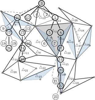
To deal with this case we proceed as follows. First, we compute the pairs of triangles whose drawings may induce a conflict. Then we construct a 2SAT formula $\phi$ that contains a Boolean variable for each triangle $\triangle\in L_{\triangle}$. The value of the variable is associated to a choice of the two possible drawings of $\triangle$: recall that an edge of $\triangle$ is part of $G_{F}$, while the vertex of $\triangle$ not incident to such an edge might be placed on either side of it. For each triangle $\triangle$ that induces a framework or an overlapping conflict in one of its two drawings, there is a clause in $\phi$ that is True if and only if the drawing of the triangle is not the one inducing a conflict. Similarly, for each pair of triangles whose drawings induce an internal or an external conflict, there is a clause in $\phi$ that is True if and only if the drawings of the triangles are not both the ones inducing a conflict. If $\phi$ is satisfiable, then there is a planar straight-line realization of $G$ which can be obtained by embedding the triangles of $L_{\triangle}$ according to the values of the variables of $\phi$. We reject the instance otherwise. We describe the algorithm in detail next.

Step D.2. Detecting internal conflicts.

We start by computing all the pairs of triangles of $L_{\triangle}$ that induce an internal conflict. This is done by traversing $T$ while processing each triangle $\triangle\in\Gamma_{F}$ as follows. We first obtain the set $L^{\prime}_{\triangle}\subseteq L_{\triangle}$ of leaf triangles that can be drawn inside $\triangle$. By Lemma 12, these triangles share an edge with $\triangle$, so they are children or siblings of $\triangle$. We then decide which pairs of leaf triangles of $L^{\prime}_{\triangle}$ induce an internal conflict inside $\triangle$, by means of Lemma 13. Since $L_{\triangle}$ is consistent, by Lemma 15 there are $O(1)$ triangles in $L^{\prime}_{\triangle}$. Hence, we process each triangle in $O(1)$ time, and the traversal takes $O(n)$ time.

Step E. Detecting overlapping conflicts.

Next, for each triangle $\triangle\in L_{\triangle}$, we detect whether any of its two drawings induces an overlapping conflict. Let $\triangle^{*}$ be the parent of $\triangle$ in $T$ and let $e$ be the edge shared by $\triangle$ and $\triangle^{*}$. Note that, since $\triangle\in L_{\triangle}$, one of the two drawings of $\triangle$ lies inside $\triangle^{*}$ and hence does not induce an overlapping conflict. We first check whether the other drawing of $\triangle$ is an internal or an outer embedding (in the latter case, we can conclude that $\triangle$ does not induce an overlapping conflict). This is equivalent to checking whether there is a triangle $\triangle_{s}$ in $\Gamma_{F}$ on the other side of $e$ with respect to $\triangle^{*}$. Note that, if such a triangle $\triangle_{s}$ exists, then it is a sibling of $\triangle$ in $T$, given that it shares the edge $e$ with $\triangle$ and that it is not the parent $\triangle^{*}$ of $\triangle$. Hence, for each of the $O(1)$ siblings of $\triangle$ in $T$, we check in $O(1)$ time whether it is a triangle in $\Gamma_{F}$ and whether it is incident to $e$. If no sibling of $\triangle$ in $T$ satisfies both checks, then we conclude that no drawing of $\triangle$ induces an overlapping conflict. Otherwise, there is a sibling of $\triangle$ in $T$ that satisfies both checks; then this sibling is the desired triangle $\triangle_{s}$ and hence the drawing of $\triangle$ outside $\triangle^{*}$ is an internal embedding of $\triangle$. Then we also check in $O(1)$ time whether $\triangle_{s}$ and the drawing of $\triangle$ outside $\triangle^{*}$ cross each other. In the positive case, we conclude that the drawing of $\triangle$ outside $\triangle^{*}$ induces an overlapping conflict, while in the negative case we conclude that it does not. Since we process each triangle $\triangle\in L_{\triangle}$ in $O(1)$ time, this step takes $O(n)$ time.

Step F. Detecting framework and external conflicts.

Detecting framework and external conflicts in linear time is more challenging than overlapping and internal conflicts. Indeed, an outer embedding of a triangle $\triangle\in L_{\triangle}$ might cross a triangle of $\Gamma_{F}$ or the outer embedding of a triangle in $L_{\triangle}$ that is far, in terms of graph-theoretic distance, from $\triangle$. Hence, the trivial solution would detect framework and external conflicts by comparing each triangle $\triangle\in L_{\triangle}$ with every triangle of $\Gamma_{F}$ and with every triangle in $L_{\triangle}$. However, this would result in a quadratic running time. In order to achieve linear running time, we decompose the plane into cells and then derive several combinatorial properties of such a decomposition, including: (i) only a linear number of cells can host conflicts and such cells can be found efficiently; (ii) conflicts can only occur between triangles in a single cell or in adjacent cells; and (iii) each cell can host only a constant number of outer embeddings of triangles from $L_{\triangle}$. The last property is only true because of the assumption $r<2$. We now describe the details of Step F.

Let $L^{\prime}_{\triangle}$ be the subset of $L_{\triangle}$ composed of those triangles that are incident to external edges of $\Gamma_{F}$. Only the outer embeddings of the triangles in $L^{\prime}_{\triangle}$ can induce framework and external conflicts. We translate the Cartesian axes so that the bottom-left corner of the bounding box of $\Gamma_{F}$ lies on the origin, and give an outer embedding to every triangle in $L^{\prime}_{\triangle}$. This results in a possibly non-planar straight-line realization $\Gamma^{\prime}_{F}$ of the graph $G^{\prime}_{F}:=G_{F}\cup L^{\prime}_{\triangle}$. Our strategy to detect external and framework conflicts is based on the construction of a linear-size “proximity” graph $H$ defined on the vertices of $G^{\prime}_{F}$. We show that, if two triangles of $L^{\prime}_{\triangle}$ induce an external conflict, then their vertices are associated either with the same node or with adjacent nodes of $H$. Similarly, if a triangle $\triangle\in L^{\prime}_{\triangle}$ induces a framework conflict by intersecting an edge $e$ of $G^{\prime}_{F}$, then the vertices of $\triangle$ and the end-vertices of $e$ are associated either with the same node or with adjacent nodes of $H$. We then detect external and framework conflicts by a linear-time traversal of $H$.

In the following, we say that a vertex of $G_{F}$ is a framework vertex and a vertex of $L^{\prime}_{\triangle}$ that is not contained in $G_{F}$ is a leaf vertex. For each leaf vertex $v$, we denote with $\triangle(v)$ the outer embedding of the triangle in $L^{\prime}_{\triangle}$ whose leaf vertex is $v$. We define the graph $H$ as follows. Consider a square grid whose cells have side length $3w_{2}$ covering the plane; see Fig. 22. We assign a label $l(v)=(i,j)$ to every vertex $v\in V(G^{\prime}_{F})$, where $i$ and $j$ respectively denote the row and the column of one of the (at most four) grid cells that contain $v$ in their interior or on their boundary. More precisely, the vertex $v$ gets the label $(\lfloor\frac{x(v)}{3w_{2}}\rfloor,\lfloor\frac{y(v)}{3w_{2}}\rfloor)$, where $(x(v),y(v))$ denotes the coordinates of $v$ in $\Gamma^{\prime}_{F}$. The graph $H$ has a node for each label assigned to at least one vertex of $G^{\prime}_{F}$, and two nodes $(i,j)$ and $(i^{\prime},j^{\prime})$ are connected if and only if $|i-i^{\prime}|\leq 1$ and $|j-j^{\prime}|\leq 1$. Note that $H$ has at most $n$ nodes and maximum degree 8, hence it has $O(n)$ edges. We say that a vertex of $G^{\prime}_{F}$ is associated with a node $\mu$ of $H$ if $\mu$ represents the cell $(i,j)$ and $l(v)=(i,j)$.

Figure 22: On the left, the straight-line realization $\Gamma^{\prime}_{F}$ of the graph $G^{\prime}_{F}:=G_{F}\cup L^{\prime}_{\triangle}$, where each triangle in $L^{\prime}_{\triangle}$ has an outer embedding. The triangles of $G_{F}$ are shown in gray, and the outer embeddings of the triangles in $L^{\prime}_{\triangle}$ are shown in white. Framework vertices are shown in white and leaf vertices are shown in blue. The grid cell filled with dashed lines is zoomed-in on the right. All the triangles in $L^{\prime}_{\triangle}$ contained in this cell can induce external or framework conflicts only with the triangles contained in the nine highlighted cells.

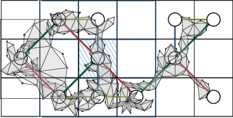
Lemma 17.

The graph $H$ satisfies the following properties:

1. For each node $\mu$ of $H$, there are $O(1)$ leaf vertices associated with $\mu$.

2. Let $\triangle_{1},\triangle_{2}$ be two triangles in $L^{\prime}_{\triangle}$. For $i=1,2$, let $\mu_{i}$ denote a node of $H$ such that at least one vertex of $\triangle_{i}$ is associated with $\mu$. If the outer embeddings of $\triangle_{1}$ and $\triangle_{2}$ induce an external conflict, then either $\mu_{1}=\mu_{2}$ or $(\mu_{1},\mu_{2})\in E(H)$.

3. Let $\triangle$ be a triangle in $L^{\prime}_{\triangle}$, and $e$ be an edge of $G_{F}$ incident to the outer face of $\Gamma_{F}$. Let $\mu$ and $\nu$ denote two nodes of $H$ such that at least one vertex of $\triangle$ is associated with $\mu$ and at least one end-vertex of $e$ is associated with $\nu$. If the outer embedding of $\triangle$ induces a framework conflict by intersecting $e$, then either $\mu_{1}=\mu_{2}$ or $(\mu_{1},\mu_{2})\in E(H)$.

Proof.

Consider any leaf vertex $v$ associated with a node $\mu$ of $H$. Let $(i,j)$ be the cell corresponding to $\mu$ and $\triangle$ be the parent triangle of the triangle in $L^{\prime}_{\triangle}$ that has $v$ as a vertex. By statement (b) of Lemma 11, we have that $\triangle$ is either a big equilateral or a tall isosceles triangle. Further, $\triangle$ is contained in the union of the nine cells $(i^{\prime},j^{\prime})$ for $|i-i^{\prime}|\leq 1$ and $|j-j^{\prime}|\leq 1$ (see the highlighted cells in Fig. 22); this is because the Euclidean distance between $v$ and every point of $\triangle$ is smaller than $2w_{2}$, while the side length of a grid cell is $3w_{2}$. Observe that the area of a big equilateral or tall isosceles triangle is larger than the area of a small equilateral triangle, which is equal to $w_{1}^{2}\sqrt{3}/4$. Moreover, any two parent triangles are interior-disjoint in $\Gamma^{\prime}_{F}$. Since the area of the union of the nine cells is $81w_{2}^{2}$, then at most $81w_{2}^{2}\frac{4}{w_{1}^{2}\sqrt{3}}=\frac{324}{\sqrt{3}}\left(\frac{w_{2}}{w_{1}}\right)^{2}\in O(r^{2})$ parent triangles are contained in the nine cells, and $O(r^{2})$ leaf vertices are associated with $\mu$. Since $r<2$, we have $O(r^{2})\in O(1)$. This proves Property (a).

To prove Property (b), suppose, for the sake of contradiction, that the outer embeddings of $\triangle_{1}$ and $\triangle_{2}$ induce an external conflict, with $\mu_{1}\neq\mu_{2}$ and $(\mu_{1},\mu_{2})\notin E(H)$. Since $\triangle_{1}$ and $\triangle_{2}$ induce an external conflict, then there is at least a point $x$ in $\triangle_{1}\cap\triangle_{2}$. Note that $x$ is at distance smaller than or equal to $w_{2}$ from the vertices of $\triangle_{1}$ and $\triangle_{2}$, which implies that every vertex of $\triangle_{1}$ is at distance smaller than or equal to $2w_{2}$ from any vertex of $\triangle_{2}$. Since there is a distance larger than or equal to $3w_{2}$ between two vertices of $G^{\prime}_{F}$ associated to non-adjacent nodes of $H$, then either $\mu_{1}=\mu_{2}$ or $(\mu_{2},\mu_{2})\in E(H)$, which is a contradiction.

Finally, Property (c) can be proved by similar arguments to those we used to prove Property (b). ∎

In order to detect external and framework conflicts, we define each node $\mu$ of $H$ representing the cell $(i,j)$ as a record storing (i) a label $l(\mu)=(i,j)$ and (ii) a list $L(\mu)$ that contains the vertices of $G^{\prime}_{F}$ associated with $\mu$. We next describe an efficient algorithm to construct $H$.

Lemma 18.

The graph $H$ can be constructed in $O(n)$ time.

Proof.

We first show how to construct the vertex set $V(H)$ of $H$.

Consider a total order $\pi$ of the vertices of $G^{\prime}_{F}$ such that, for any two vertices $u$ and $v$ with $l(u)=(i_{u},j_{u})$ and $l(v)=(i_{v},j_{v})$, it holds that $u$ precedes $v$ in the order if (i) $i_{u}<i_{v}$ or (ii) $i_{u}=i_{v}$ and $j_{u}<j_{v}$; if $i_{u}=i_{v}$ and $j_{u}=j_{v}$, then $u$ and $v$ are in any relative order in $\pi$. Since $G^{\prime}_{F}$ is connected and any edge of $G^{\prime}_{F}$ has length at most $w_{2}$, then $i,j\leq\frac{w_{2}n}{3w_{2}}=\frac{1}{3}n$ for any label $(i,j)$. Hence, we can compute $\pi$ in $O(n)$ time by means of counting sort.

We process the vertices of $G^{\prime}_{F}$ in the order in which they appear in $\pi$. Let $s$ be the first vertex in the order $\pi$. We create a node $\nu$ of $H$, set $l(\nu)=l(s)$, and add $s$ to $L(\nu)$. Let now $v$ be the currently considered vertex of $\pi$ and let us denote by $\mu$ the last created node of $H$. If $l(v)=l(\mu)$, then we add $v$ to $L(\mu)$; otherwise, we create a node $\mu^{\prime}$ of $H$, set $l(\mu^{\prime})=l(v)$, and add $v$ to $L(\mu^{\prime})$. Note that, if two vertices of $G^{\prime}_{F}$ have the same label, then they are consecutive in $\pi$. Therefore, the above procedure creates a new node of $H$ for each label of a vertex of $G^{\prime}_{F}$, and vertices with the same label $(i,j)$ are all placed in the list $L(\mu)$ of the node $\mu$ such that $l(\mu)=(i,j)$. The procedure can clearly be performed in overall $O(n)$ time.

We now show how to construct the edge set $E(H)$ of $H$.

We define a partition of $E(H)$ into four subsets $E_{-},E_{|},E_{/},E_{\backslash}$; refer to Fig. 23. Consider any edge $(\mu,\nu)\in E(H)$, where we denote $l(\mu)=(i_{\mu},j_{\mu})$ and $l(\nu)=(i_{\nu},j_{\nu})$. Then $(\mu,\nu)$ belongs to $E_{-}$, $E_{|}$, $E_{/}$, or $E_{\backslash}$, depending on whether $(\mu,\nu)$ satisfies Property $P_{-}$, $P_{|}$, $P_{/}$, or $P_{\backslash}$, respectively, where:

$P_{-}$:

$i_{\mu}=i_{\nu}$ and $|j_{\mu}-j_{\nu}|=1$,

$P_{|}$:

$j_{\mu}=j_{\nu}$ and $|i_{\mu}-i_{\nu}|=1$,

$P_{/}$:

either $i_{\mu}-i_{\nu}=j_{\mu}-j_{\nu}=1$ or $i_{\mu}-i_{\nu}=j_{\mu}-j_{\nu}=-1$, and

$P_{\backslash}$:

either $i_{\mu}-i_{\nu}=1$ and $j_{\mu}-j_{\nu}=-1$ or $i_{\mu}-i_{\nu}=-1$ and $j_{\mu}-j_{\nu}=1$.

Figure 23: Construction of the set of edges $E(H)$. The edges on the sets $E_{-},E_{|},E_{/}$, and $E_{\backslash}$ are shown in yellow, blue, green, and red, respectively.

In order to construct the sets $E_{-},E_{|},E_{/}$, and $E_{\backslash}$, we define four total orders $\pi_{-}$, $\pi_{|}$, $\pi_{/}$, and $\pi_{\backslash}$ of the nodes of $H$, respectively. For any two nodes $\mu$ and $\nu$ of $H$, it holds that $\mu$ precedes $\nu$ in $\pi_{-}$, $\pi_{|}$, $\pi_{/}$, and $\pi_{\backslash}$ if and only if the following conditions hold, respectively:

$C_{-}$:

either $i_{\mu}<i_{\nu}$ or $i_{\mu}=i_{\nu}$ and $j_{\mu}<j_{\nu}$,

$C_{|}$:

either $j_{\mu}<j_{\nu}$ or $j_{\mu}=j_{\nu}$ and $i_{\mu}<i_{\nu}$,

$C_{/}$:

either $i_{\mu}-j_{\mu}<i_{\nu}-j_{\nu}$ or $i_{\mu}-j_{\mu}=i_{\nu}-j_{\nu}$ and $i_{\mu}<i_{\nu}$, or

$C_{\backslash}$:

either $i_{\mu}+j_{\mu}<i_{\nu}+j_{\nu}$ or $i_{\mu}+j_{\mu}=i_{\nu}+j_{\nu}$ and $i_{\mu}<i_{\nu}$.

We construct the set $E_{i}$ with $i\in\{-,|,/,\backslash\}$ as follows. First, we compute the total order $\pi_{i}$ of the nodes of $H$ for which condition $C_{i}$ holds for any pair $(\mu,\nu)$ of nodes such that $\mu$ precedes $\nu$ in $\pi_{i}$. Similarly as in the construction of $\pi$, the order $\pi_{i}$ can be computed in $O(n)$ time by means of counting sort. Then we process the nodes of $V(H)$ in the order $\pi_{i}$ and add a new edge $(\mu,\nu)$ to $E_{i}$ whenever condition $P_{i}$ holds for two nodes $\mu$ and $\nu$ such that $\mu$ immediately precedes $\nu$ in $\pi_{i}$. Since, by construction, nodes that are adjacent in $E_{i}$ are consecutive in $\pi_{i}$, it follows that the above procedure correctly computes each set $E_{i}$. Clearly, the procedure can be performed in overall $O(n)$ time. This concludes the construction of $H$. ∎

We now describe an algorithm, which we call ConflictFinder, to detect external and framework conflicts. Broadly speaking, the algorithm performs two linear-time traversals of the edges of $H$. In the first traversal, we detect external conflicts. When processing the edge $(\mu,\nu)\in E(H)$ we detect intersections between the triangles of $L^{\prime}_{\triangle}$ whose leaf vertices are contained in $L(\mu)\cup L(\nu)$. In the second traversal, we detect framework conflicts. In this case, when processing the edge $(\mu,\nu)\in E(H)$ we detect intersections between the triangles of $L^{\prime}_{\triangle}$ and the edges of $G^{\prime}_{F}$ whose leaf and framework end-vertices, respectively, are contained in $L(\mu)\cup L(\nu)$.

The algorithm consists of the following steps:

1. Compute the drawing $\Gamma^{\prime}_{F}$ of $G^{\prime}_{F}$ and the auxiliary graph $H$ as described above.

2. For every framework vertex $v$, create the list $L_{E}(v)$ of the two edges of $\Gamma_{F}$ incident to both $v$ and the outer face of $\Gamma_{F}$.

3. For every node $\mu\in V(H)$, create the lists $L_{\ell}(\mu)$ and $L_{F}(\mu)$ of leaf and framework vertices contained in $L(\mu)$, respectively.

4. Detect which triangles of $L^{\prime}_{\triangle}$ induce external conflicts as follows. Let $\mathcal{E}_{\ell}=\{(u,v)\in L_{\ell}(\mu)\times\{L_{\ell}(\mu)\cup L_{\ell}(\nu)\}\,|\,(\mu,\nu)\in E(H)\}$. For every pair of vertices $(u,v)\in\mathcal{E}_{\ell}$, test if $\triangle(u)$ and $\triangle(v)$ intersect each other. In the positive case, the triangles $\triangle(u)$ and $\triangle(v)$ induce an external conflict.

5. Detect which triangles of $L^{\prime}_{\triangle}$ induce framework conflicts as follows. Let $\mathcal{E}_{F}=\{(u,v)\in L_{F}(\mu)\times\{L_{\ell}(\mu)\cup L_{\ell}(\nu)\}\,|\,(\mu,\nu)\in E(H)\}$. For every pair of vertices $(u,v)\in\mathcal{E}_{F}$, test if there is an edge $e\in L_{E}(u)$ such that $e$ intersects $\triangle(v)$. In the positive case, the triangle $\triangle(v)$ induces a framework conflict with the edge $e$.

The correctness and complexity of the algorithm are proved in the following lemma.

Lemma 19.

The algorithm ConflictFinder detects all the external and framework conflicts in $O(n)$ time.

Proof.

We first prove the correctness of the algorithm. Consider first the detection of external conflicts. Let $u$ and $v$ be two leaf vertices associated respectively to two nodes $\mu$ and $\nu$. Remember that $\triangle(u)$ and $\triangle(v)$ induce an external conflict if and only if they intersect each other. Then, by Property (b) of Lemma 17, we have that either $\mu=\nu$ or $(\mu,\nu)\in E(H)$. Since in Step 4 the algorithm processes each pair of leaf triangles whose leaf vertices are associated with the same node of $H$ or with adjacent nodes of $H$, it follows that all the external conflicts are being detected.

Consider now the detection of framework conflicts. Let $u$ be a framework vertex associated to a node $\mu$, let $v$ be a leaf vertex associated to a node $\nu$, and $e$ be an edge in $L_{E}(u)$. Remember that $\triangle(v)$ induces a framework conflict with $e$ if and only if $\triangle(v)$ and $e$ intersect each other. Then, by Property (c) of Lemma 17, we have that either $\mu=\nu$ or $(\mu,\nu)\in E(H)$. Since in Step 5 the algorithm processes each pair composed of a framework and a leaf vertex that are associated either with the same node of $H$ or with adjacent nodes of $H$, it follows that all the framework conflicts are being detected.

We now bound the time complexity of the algorithm. This is done by bounding the time complexity of each of the Steps 1–5.

• Since there are $O(n)$ triangles in $L^{\prime}_{\triangle}$, we have that $\Gamma_{F}$ can be extended to $\Gamma^{\prime}_{F}$ in $O(n)$ time. Furthermore, the graph $H$ can be computed in $O(n)$ time by Lemma 18. Hence Step 1 takes $O(n)$ time.

• Step 2 takes $O(n)$ time since the boundary of the outer face of $\Gamma_{F}$ consists of $O(n)$ line segments.

• Step 3 takes also $O(n)$ time, since $H$ has at most $n$ nodes, and every vertex $v$ of $G^{\prime}_{F}$ is contained in the list $L(\mu)$ of a single node $\mu$ of $H$.

• The time complexity of Step 4 is bounded by $O(|\mathcal{E}_{\ell}|)$. Note that $H$ contains $O(n)$ edges; moreover, for every node $\mu$ of $H$, the list $L_{\ell}(\mu)$ contains $O(1)$ leaf vertices, by Property (a) of Lemma 17. Hence $\mathcal{E}_{\ell}$ contains $O(n)$ pairs of vertices and Step 4 takes $O(n)$ time.

• Finally, the time complexity of Step 5 is bounded by $O(|\mathcal{E}_{F}|)$. In this case, even though $\Theta(n)$ framework vertices might be associated with the same node of $H$, each framework vertex appears in $O(1)$ pairs of $\mathcal{E}_{F}$; namely, if a framework vertex $u$ is associated with a node $\mu$ of $H$, then it only appears in the pairs $(u,v)$ of $\mathcal{E}_{F}$ such that the leaf vertex $v$ is associated either with $\mu$ or with one of the (at most $8$) neighbors of $\mu$ in $H$. By Property (a) of Lemma 17, there are $O(1)$ leaf vertices associated with the same node of $H$, hence $\mathcal{E}_{F}$ contains $O(n)$ pairs of vertices and Step 5 takes $O(n)$ time.

This concludes the proof of the time complexity and hence the proof of the lemma. ∎

Step G. Extending $\Gamma_{F}$ to a planar straight-line realization of $G$.

The final step is to draw the triangles of $L_{\triangle}$ in $\Gamma_{F}$ without inducing conflicts, so that the resulting drawing remains planar. We decide if this is possible by means of a 2SAT formula. Each leaf triangle $\triangle_{i}\in L_{\triangle}$ can have two embeddings (which differ from each other for the position of the leaf vertex of $\triangle_{i}$). We arbitrarily associate each embedding with a distinct truth value of a suitable Boolean variable, and construct the clauses of the formula as follows:

• If a drawing of $\triangle_{i}$ induces an overlapping conflict, then we introduce a clause $(\neg\ell_{i})$, where $\ell_{i}$ is the literal that is True when $\triangle_{i}$ has the drawing that induces an overlapping conflict.

• If $\triangle_{i}$ induces a framework conflict, we introduce a clause $(\neg\ell_{i})$, where $\ell_{i}$ is the literal that is True when $\triangle_{i}$ has an outer embedding.

• If two leaf triangles $\triangle_{i},\triangle_{j}\in L_{\triangle}$ induce an internal conflict inside a triangle $\triangle\in\Gamma_{F}$, we introduce a clause $(\neg\ell_{i}\vee\neg\ell_{j})$, where $\ell_{i}$ (resp. $\ell_{j}$) is the literal that is True when $\triangle_{i}$ (resp. $\triangle_{j}$) is drawn inside $\triangle$.

• If two leaf triangles $\triangle_{i},\triangle_{j}\in L_{\triangle}$ induce an external conflict, we introduce a clause $(\neg\ell_{i}\vee\neg\ell_{j})$, where $\ell_{i}$ (resp. $\ell_{j}$) is the literal that is True when $\triangle_{i}$ (resp. $\triangle_{j}$) has an outer embedding.

Let $\phi$ be the 2SAT formula produced by the clauses introduced as described above. Clearly, the clauses of $\phi$ describe all and only the overlapping, framework, internal, and external conflicts defined in Section 5.2. Moreover, since there are $O(n)$ triangles in $L_{\triangle}$, the number of framework and overlapping conflicts is in $O(n)$. Further, since $H$ has $O(n)$ vertices and edges, by Lemmas 15 and 17 the number of internal and external conflicts is in $O(n)$, respectively. It follows that $\phi$ contains $O(n)$ clauses. The following lemma shows that a solution to $\phi$ corresponds to a planar straight-line realization of $G$.

Lemma 20.

The formula $\phi$ is satisfiable if and only if $\Gamma_{F}$ can be extended to a planar straight-line realization of $G$. Also, if $\phi$ is satisfiable, then such a planar straight-line realization can be constructed in $O(n)$ time.

Proof.

We prove the two directions separately.

$(\Longrightarrow)$ Assume that $\phi$ is satisfiable. We show that $\Gamma_{F}$ can be extended to a planar straight-line realization of $G$. Consider a truth assignment for the Boolean variables that satisfies $\phi$. The variables of $\phi$ are in one to one correspondence with the triangles of $L_{\triangle}$. We draw in $\Gamma_{F}$ each triangle $\triangle_{i}\in L_{\triangle}$ with the embedding associated with the truth value of the variable corresponding to $\triangle_{i}$ in the satisfying assignment for $\phi$. This can clearly be done in $O(1)$ time per triangle in $L_{\triangle}$, hence in overall $O(n)$ time. Since each clause of $\phi$ is satisfied, it follows that $\triangle_{i}$ is drawn in $\Gamma_{F}$ without inducing conflicts. Since this is true for every $\triangle_{i}\in L_{\triangle}$, it follows that the resulting straight-line realization of $G$ is planar. Furthermore, such a realization can be constructed in $O(n)$ time since there are $O(n)$ clauses in $\phi$.

$(\Longleftarrow)$ Let $\Gamma$ be a planar straight-line realization of $G$. We show that $\phi$ is satisfiable. The embedding in $\Gamma$ of each triangle $\triangle_{i}\in L_{\triangle}$ identifies a truth value for the corresponding variable in $\phi$, and thus, a truth assignment for $\phi$. Such an assignment satisfies $\phi$ since an unsatisfied clause would imply that we have either an overlapping, or a framework, or an internal, or an external conflict, which in turn implies that the boundary of some triangle $\triangle_{i}\in L_{\triangle}$ crosses the boundary of a triangle of $\Gamma_{F}$ or the boundary of another triangle of $L_{\triangle}$, contradicting the fact that $\Gamma$ is planar. This concludes the proof. ∎

By the discussion in Steps D.2, E, and F, we have that $\phi$ can be constructed in $O(n)$ time. Further, as argued above, $\phi$ contains $O(n)$ clauses. We can therefore test whether $\phi$ is satisfiable in $O(n)$ time [6]. If $\phi$ is not satisfiable, we reject the instance. Otherwise, we extend $\Gamma_{F}$ to a planar straight-line realization of $G$ in $O(n)$ time as described in the proof of Lemma 20. This concludes the proof of Theorem 5.2.

6 Maximal Outerplanar Graphs

In this section we study the FEPR problem for weighted outerplanar $2$-trees, that is, for weighted maximal outerplanar graphs. While we could not establish the computational complexity of the FEPR problem for general maximal outerplanar graphs, we can prove the following two theorems.

Theorem 6.1.

Let $G$ be an $n$-vertex weighted maximal outerpath. There exists an $O(n)$-time algorithm that tests whether $G$ admits a planar straight-line realization and, in the positive case, constructs such a realization.

Theorem 6.2.

Let $G$ be an $n$-vertex weighted maximal outerpillar. There exists an $O(n^{3})$-time algorithm that tests whether $G$ admits a planar straight-line realization and, in the positive case, constructs such a realization.

(a)

(b)

(c)

Figure 24: (a) and (b) show two $e$-outer realizations $\Gamma$ and $\Gamma^{\prime}$ of a weighted $2$-tree. The gray regions show $\mathcal{I}_{\Gamma}$ and $\mathcal{I}_{\Gamma^{\prime}}$. We have that $\Gamma$ is $e$-smaller than $\Gamma^{\prime}$. Indeed, as shown in (c), $\Gamma$ can be rotated, translated, and reflected so that the representation of $e$ coincides with the one in $\Gamma^{\prime}$ and so that its interior is a subset of the interior of $\Gamma^{\prime}$.

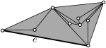
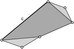
Before proving Theorems 6.1 and 6.2, we establish some notation and definitions that are common to both proofs. Let $G$ be a weighted $2$-tree. For a planar straight-line realization $\Gamma$ of $G$, the interior of $\Gamma$, denoted by $\mathcal{I}_{\Gamma}$, is the complement of the outer face of $\Gamma$, i.e., the union of the closure of the internal faces of $\Gamma$. Let $e$ be an edge of $G$. An $e$-outer realization of $G$ is a planar straight-line realization of $G$ such that $e$ is incident to its outer face. Given two $e$-outer realizations $\Gamma$ and $\Gamma^{\prime}$ of $G$, we say that $\Gamma$ is $e$-smaller than $\Gamma^{\prime}$ if there exists an $e$-outer realization $\Gamma^{\prime\prime}$ that can be obtained by a rigid transformation of $\Gamma$ such that the end-vertices of $e$ lie at the same points in $\Gamma^{\prime\prime}$ and in $\Gamma^{\prime}$ and such that $\mathcal{I}_{\Gamma^{\prime\prime}}\subseteq\mathcal{I}_{\Gamma^{\prime}}$ (see Fig. 24); that is $\Gamma$ is $e$-smaller than $\Gamma^{\prime}$ if it can be rotated, translated, and possibly reflected so that the representation of $e$ coincides with the one in $\Gamma^{\prime}$ and so that its interior is a subset of the interior of $\Gamma^{\prime}$. A set $\mathcal{R}$ of $e$-outer realizations of $G$ is $e$-optimal if, for every $e$-outer realization $\Gamma^{\prime}$ of $G$, there exists an $e$-outer realization $\Gamma$ of $G$ in $\mathcal{R}$ such that $\Gamma$ is $e$-smaller than $\Gamma^{\prime}$. An $e$-outer realization $\Gamma$ of $G$ is $e$-optimal if the set $\{\Gamma\}$ is $e$-optimal.

The following lemma will be very useful; see Fig. 25. Roughly speaking, it asserts that, in order to construct a planar straight-line realization of a weighted $2$-tree, for certain subgraphs it is not a loss of generality to use realizations that are “as $e$-small as possible”.

Lemma 21.

Let $G$ be a weighted $2$-tree that admits a planar straight-line realization $\mathcal{G}$. Let $H$ and $K$ be two subgraphs of $G$ that satisfy the following properties:

• $H$ and $K$ are weighted $2$-trees;

• $H\cup K=G$ (that is, every vertex and edge of $G$ is in $H$ or in $K$);

• $H\cap K=e$ (that is, $H$ and $K$ share an edge $e$, the end-vertices of $e$, and no other edge or vertex);

• the restriction $\mathcal{H}$ of $\mathcal{G}$ to $H$ is an $e$-outer realization of $H$; and

• no vertex of $K$ lies inside an internal face of $\mathcal{H}$ in $\mathcal{G}$.

Let $\mathcal{H}^{\prime}$ be any $e$-outer realization of $H$ that is $e$-smaller than $\mathcal{H}$. Then it is possible to replace $\mathcal{H}$ with an $e$-outer realization of $H$ that can be obtained by a rigid transformation of $\mathcal{H}^{\prime}$ in such a way that the resulting straight-line realization of $G$ is planar.

(a)

(b)

Figure 25: (a) The drawing $\mathcal{G}$; the set $\mathcal{I}_{\mathcal{H}}$ is shaded gray. The region with dark gray strips is the face $f$ of $\mathcal{K}$. (b) The drawing obtained from $\mathcal{G}$ by replacing $\mathcal{H}$ with $\mathcal{H}^{\prime\prime}$; the set $\mathcal{I}_{\mathcal{H}^{\prime\prime}}$ is gray.

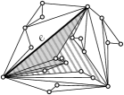
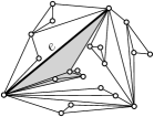
Proof.

Let $\mathcal{K}$ be the restriction of $\mathcal{G}$ to $K$. Assume that $H$ has more than two vertices, as otherwise $H$ contains a single edge, hence $\mathcal{H}^{\prime}$ can be obtained by a rigid transformation of $\mathcal{H}$ and the statement is trivial. By assumption, no vertex of $K$ lies in $\mathcal{I}_{\mathcal{H}}$; further, $H$ is biconnected, by Property (P1) of a $2$-tree. It follows that there is a face $f$ of $\mathcal{K}$ that contains $\mathcal{H}$ entirely, except for the edge $e$ and its end-vertices, which are shared by $H$ and $K$. By assumption, there exists an $e$-outer realization $\mathcal{H}^{\prime\prime}$ of $H$ that can be obtained by a rigid transformation of $\mathcal{H}^{\prime}$ such that $\mathcal{I}_{\mathcal{H}^{\prime\prime}}\subseteq\mathcal{I}_{\mathcal{H}}$, hence the part of $\mathcal{H}^{\prime\prime}$ different from the edge $e$ does not intersect $\mathcal{K}$; the edge $e$ does not intersect $\mathcal{K}$ either, as it is part of it and $\mathcal{K}$ is planar. Hence, the straight-line realization of $G$ resulting from the replacement of $\mathcal{H}$ with $\mathcal{H}^{\prime\prime}$ in $\mathcal{G}$ is planar. ∎

We are now ready to prove Theorems 6.1 and 6.2.

Proof of Theorem 6.1. Let $G=(V,E,\lambda)$ be an $n$-vertex weighted maximal outerpath (as the one in Fig. 26) and let $\mathcal{O}$ be its outerplane embedding, which can be found in $O(n)$ time [21, 38, 50]. Since $G$ is an outerpath, its dual tree is a path, which we denote by $P:=(p_{1},\dots,p_{k})$, where $k=n-2$; note that $P$ can be easily recovered from $\mathcal{O}$ in $O(n)$ time. Each node $p_{i}$ of $P$ corresponds to an internal face of $\mathcal{O}$; we denote by $c_{i}$ the $3$-cycle of $G$ bounding such a face; each cycle $c_{i}$ has a unique (planar) straight-line realization (up to a rigid transformation), which we denote by $\mathcal{C}_{i}$. Further, for $i=1,\dots,k-1$, let $e_{i}$ be the edge of $G$ that is dual to the edge $(p_{i},p_{i+1})$ of $P$; note that $e_{i}$ is an internal edge of $\mathcal{O}$.

Figure 26: The outerplane embedding of an outerpath. The gray face is the one bounded by $c_{x}$. The graphs $G_{1}$ and $G_{2}$ are enclosed inside fat curves.

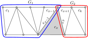
Let $x\in\{1,\dots,k\}$ be an index such that the sum of the lengths of the edges of $c_{x}$ is maximum. Let $G_{1}$ be the subgraph of $G$ composed of the $3$-cycles $c_{1},c_{2},\dots,c_{x-1}$ and let $G_{2}$ be the subgraph of $G$ composed of the $3$-cycles $c_{x+1},c_{x+2},\dots,c_{k}$. One of these graphs might be undefined if $x=1$ or $x=k$; however, in the following, we assume that $1<x<k$ as the arguments for the cases $x=1$ and $x=k$ are analogous and actually simpler. Note that $G_{1}$ and $G_{2}$ are maximal outerpaths.

Assume that a planar straight-line realization $\Gamma$ of $G$ exists; for $i=1,2$, let $\Gamma_{i}$ be the restriction of $\Gamma$ to $G_{i}$. Since the sum of the lengths of the edges of $c_{x}$ is maximum among all the $3$-cycles of $G$, it follows that $c_{x}$ does not lie inside any $3$-cycle of $G$ in $\Gamma$; hence, $\Gamma_{1}$ is an $e_{x-1}$-outer realization of $G_{1}$ and $\Gamma_{2}$ is an $e_{x}$-outer realization of $G_{2}$.

A key ingredient of our algorithm is the fact that, if there exists an $e_{x-1}$-outer realization of $G_{1}$ (resp. an $e_{x}$-outer realization of $G_{2}$), then there exists an $e_{x-1}$-optimal realization of $G_{1}$ (resp. an $e_{x}$-optimal realization of $G_{2}$). Indeed, in the following, we show an $O(n)$-time algorithm that either (i) concludes that $G_{1}$ admits no $e_{x-1}$-outer realization or that $G_{2}$ admits no $e_{x}$-outer realization, and thus $G$ admits no planar straight-line realization, or (ii) constructs an $e_{x-1}$-optimal realization $\Gamma_{1}$ of $G_{1}$ and its plane embedding $\mathcal{E}(\Gamma_{1})$, and an $e_{x}$-optimal realization $\Gamma_{2}$ of $G_{2}$ and its plane embedding $\mathcal{E}(\Gamma_{2})$.

Figure 27: The four different ways to combine $\Gamma_{1}$ and $\Gamma_{2}$ with $\mathcal{C}_{x}$. In this example, the first realization is not planar, while the other three are.

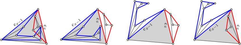
In view of the argument above, the existence of such an algorithm suffices to conclude the proof of the theorem. Indeed, if the algorithm concludes that $G_{1}$ admits no $e_{x-1}$-outer realization or that $G_{2}$ admits no $e_{x}$-outer realization, then $G$ admits no planar straight-line realization. Otherwise, the algorithm constructs an $e_{x-1}$-optimal realization $\Gamma_{1}$ of $G_{1}$, together with its plane embedding $\mathcal{E}(\Gamma_{1})$, and an $e_{x}$-optimal realization $\Gamma_{2}$ of $G_{2}$, together with its plane embedding $\mathcal{E}(\Gamma_{2})$. Then, in order to test whether $G$ admits a planar straight-line realization, we consider the unique (up to a rigid transformation) planar straight-line realization $\mathcal{C}_{x}$ of $c_{x}$ and we try to combine it with $\Gamma_{1}$ and $\Gamma_{2}$ (see Fig. 27). This combination can be done in four ways. Indeed, once $\Gamma_{1}$ and $\mathcal{C}_{x}$ coincide on the representation of $e_{x-1}$, it still remains to decide whether the vertex of $c_{x-1}$ not incident to $e_{x-1}$ and the vertex of $c_{x}$ not incident to $e_{x-1}$ lie on different sides or on the same side of the line through $e_{x-1}$, and similarly for $\Gamma_{2}$ and $\mathcal{C}_{x}$. These two independent choices result in four straight-line realizations of $G$. Each of these realizations, say $\Gamma$, can be constructed in $O(n)$ time; further, its plane embedding $\mathcal{E}(\Gamma)$ can also be constructed in $O(n)$ time from $\mathcal{E}(\Gamma_{1})$ and $\mathcal{E}(\Gamma_{2})$. Then it can be tested in $O(n)$ time whether $\Gamma$ is a planar straight-line realization respecting $\mathcal{E}(\Gamma)$, due to Theorem 3.1. If (at least) one of the four realizations is planar, then it is the desired planar straight-line realization of $G$. Otherwise, we claim that there exists no planar straight-line realization of $G$. For a contradiction, assume that there exists such a realization, and denote it by $\Gamma$. Since $\Gamma_{1}$ is $e_{x-1}$-optimal, it is $e_{x-1}$-smaller than the restriction of $\Gamma$ to $G_{1}$; hence, we can apply Lemma 21 with $H=G_{1}$, $K=G_{2}\cup c_{x}$, $\mathcal{G}=\Gamma$, $e=e_{x-1}$, and $\mathcal{H}^{\prime}=\Gamma_{1}$, in order to obtain a planar straight-line realization $\Gamma^{\prime}$ of $G$ whose restriction to $G_{1}$ is $\Gamma_{1}$. Further, since $\Gamma_{2}$ is $e_{x}$-optimal, it is $e_{x}$-smaller than the restriction of $\Gamma^{\prime}$ to $G_{2}$; hence, we can apply Lemma 21 with $H=G_{2}$, $K=G_{1}\cup c_{x}$, $\mathcal{G}=\Gamma^{\prime}$, $e=e_{x}$, and $\mathcal{H}^{\prime}=\Gamma_{2}$, in order to obtain a planar straight-line realization $\Gamma^{\prime\prime}$ of $G$ whose restriction to $G_{1}$ is $\Gamma_{1}$ and whose restriction to $G_{2}$ is $\Gamma_{2}$; however, this is one of the four straight-line realizations for which the planarity testing was negative, a contradiction.

It remains show an $O(n)$-time algorithm that either concludes that $G_{1}$ admits no $e_{x-1}$-outer realization, or determines an $e_{x-1}$-optimal realization of $G_{1}$. A very similar application of the algorithm allows us to either conclude that $G_{2}$ admits no $e_{x}$-outer realization or to determine an $e_{x}$-optimal realization of $G_{2}$.

For $i=1,\dots,x-1$, let $G^{i}_{1}$ be the subgraph of $G_{1}$ composed of the $3$-cycles $c_{1},c_{2},\dots,c_{i}$; note that $G^{x-1}_{1}=G_{1}$. A key observation for our algorithm is the following. Assume that an $e_{x-1}$-outer realization $\Gamma_{1}$ of $G_{1}$ exists; let $\Gamma^{i}_{1}$ be the restriction of $\Gamma_{1}$ to $G^{i}_{1}$. Then $\Gamma^{i}_{1}$ is an $e_{i}$-outer realization of $G^{i}_{1}$. This is trivial when $i=x-1$; further, when $i<x-1$, if $e_{i}$ were not incident to the outer face of $\Gamma^{i}_{1}$, then $e_{x-1}$ could not be incident to the outer face of $\Gamma_{1}$ without violating the planarity of $\Gamma_{1}$.

Our algorithm works by induction on $i$ in order to either conclude that $G^{i}_{1}$ admits no $e_{i}$-outer realization (and thus $G_{1}$ admits no $e_{x-1}$-outer realization), or to determine an $e_{i}$-optimal realization $\Gamma^{i}_{1}$ of $G^{i}_{1}$. This is trivial when $i=1$, namely $G^{1}_{1}$ is the $3$-cycle $c_{1}$ which has a unique planar straight-line realization $\Gamma^{1}_{1}:=\mathcal{C}_{1}$, up to a rigid transformation; then $\Gamma^{1}_{1}$ is indeed an $e_{1}$-optimal realization.

Assume that we have an $e_{i-1}$-optimal realization $\Gamma^{i-1}_{1}$ of $G^{i-1}_{1}$, for some $i\in\{2,\dots,x-1\}$; indeed, if we already concluded that $G_{1}$ admits no $e_{x-1}$-outer realization, there is nothing else to do.

Note that the cycles $c_{i-1}$ and $c_{i}$ share the edge $e_{i-1}$; let $v_{i-1}$ and $v_{i}$ be the vertices of $c_{i-1}$ and $c_{i}$, respectively, not incident to $e_{i-1}$. Any straight-line realization of $G^{i}_{1}$ is of one of two types: it is a different-side realization if $v_{i-1}$ and $v_{i}$ lie on different sides of the line through $e_{i-1}$, while it is a same-side realization if $v_{i-1}$ and $v_{i}$ lie on the same side of the line through $e_{i-1}$.

In order to determine whether an $e_{i}$-outer realization of $G^{i}_{1}$ exists, we combine $\Gamma^{i-1}_{1}$ with $\mathcal{C}_{i}$ in two ways, so to form a different-side realization and a same-side realization. Namely, $G^{i-1}_{1}$ and $c_{i}$ share the edge $e_{i-1}$; hence, once $\Gamma^{i-1}_{1}$ and $\mathcal{C}_{i}$ coincide on the representation of $e_{i-1}$, it still remains to decide whether $v_{i-1}$ and $v_{i}$ lie on different sides or on the same side of the line through $e_{i-1}$. This choice leads to two straight-line realizations of $G^{i}_{1}$, which we respectively denote by $\Gamma^{i,a}_{1}$ and $\Gamma^{i,b}_{1}$.

We check each of $\Gamma^{i,a}_{1}$ and $\Gamma^{i,b}_{1}$ for planarity and discard each realization that is not planar. Further, if $\Gamma^{i,b}_{1}$ was not discarded, then the triangles $\mathcal{C}_{i-1}$ and $\mathcal{C}_{i}$ are one nested into the other one (except for the edge $e_{i-1}$, which is common to both triangles) in such a realization. If $\mathcal{C}_{i}$ is nested into $\mathcal{C}_{i-1}$, then we discard $\Gamma^{i,b}_{1}$, as it is not an $e_{i}$-outer realization of $G^{i}_{1}$. We have now three cases:

• If we did not discard $\Gamma^{i,b}_{1}$, then we set $\Gamma^{i}_{1}=\Gamma^{i,b}_{1}$. Indeed, if we did not discard $\Gamma^{i,b}_{1}$, then $\Gamma^{i,b}_{1}$ is a planar straight-line realization of $G^{i}_{1}$ in which $\mathcal{C}_{i-1}$ is nested into $\mathcal{C}_{i}$; this implies that all of $\Gamma^{i-1}_{1}$ lies inside $\mathcal{C}_{i}$, hence $\mathcal{I}_{\Gamma^{i}_{1}}$ coincides with the closure of the interior of $\mathcal{C}_{i}$. It follows that $\Gamma^{i}_{1}$ is an $e_{i}$-optimal realization of $G^{i}_{1}$, given that in any planar straight-line realization of $G^{i}_{1}$ the cycle $c_{i}$ is represented by the triangle $\mathcal{C}_{i}$.

• If we discarded $\Gamma^{i,b}_{1}$ but we did not discard $\Gamma^{i,a}_{1}$, then we set $\Gamma^{i}_{1}=\Gamma^{i,a}_{1}$. We prove that $\Gamma^{i}_{1}$ is an $e_{i}$-optimal realization of $G^{i}_{1}$.

  First, we prove that there exists no same-side $e_{i}$-outer realization of $G^{i}_{1}$. This is obvious if $\Gamma^{i,b}_{1}$ was discarded because $\mathcal{C}_{i}$ is nested into $\mathcal{C}_{i-1}$, as the same would be true in any same-side realization of $G^{i}_{1}$. Suppose hence that $\Gamma^{i,b}_{1}$ was discarded because it is not planar and suppose, for a contradiction, that there exists a same-side $e_{i}$-outer realization $\Psi^{i}_{1}$ of $G^{i}_{1}$. Since $\Gamma^{i-1}_{1}$ is $e_{i-1}$-optimal, it is $e_{i-1}$-smaller than the restriction of $\Psi^{i}_{1}$ to $G^{i-1}_{1}$; hence, we can apply Lemma 21 with $H=G^{i-1}_{1}$, $K=c_{i}$, $\mathcal{G}=\Psi^{i}_{1}$, $e=e_{i-1}$, and $\mathcal{H}^{\prime}=\Gamma^{i-1}_{1}$, in order to obtain a planar straight-line realization $\Gamma^{i,*}_{1}$ of $G$ whose restriction to $G^{i-1}_{1}$ is $\Gamma^{i-1}_{1}$. Since $\Psi^{i}_{1}$ is a same-side realization of $G^{i}_{1}$, we have that $\Gamma^{i,*}_{1}$ is also a same-side realization of $G^{i}_{1}$. Hence, $\Gamma^{i,*}_{1}$ is the same realization as $\Gamma^{i,b}_{1}$, a contradiction to the fact that $\Gamma^{i,b}_{1}$ is not planar.

  Second, since we did not discard $\Gamma^{i,a}_{1}$, we have that $\Gamma^{i}_{1}=\Gamma^{i,a}_{1}$ is planar. This, together with the fact that $\Gamma^{i}_{1}$ is a different-side realization, implies that $\Gamma^{i}_{1}$ is an $e_{i}$-outer realization. The proof that $\Gamma^{i}_{1}$ is an $e_{i}$-optimal realization of $G^{i}_{1}$ easily follows by induction. Namely, as proved above, any $e_{i}$-outer realization of $G^{i}_{1}$ is a different-side realization. Consider any such realization $\Psi^{i}_{1}$ and let $\Psi^{i-1}_{1}$ be the restriction of $\Psi^{i}_{1}$ to the vertices and edges of $G^{i-1}_{1}$. By induction, we have that $\Gamma^{i-1}_{1}$ is $e_{i-1}$-smaller than $\Psi^{i-1}_{1}$, hence $\Gamma^{i}_{1}$ is $e_{i}$-smaller than $\Psi^{i}_{1}$, given that the realization $\mathcal{C}_{i}$ of $c_{i}$ coincides in $\Gamma^{i}_{1}$ and $\Psi^{i}_{1}$.

• Finally, if we discarded both $\Gamma^{i,a}_{1}$ and $\Gamma^{i,b}_{1}$, we conclude that there exists no $e_{i}$-outer realization of $G^{i}_{1}$. Namely, the proof that there exists no same-side $e_{i}$-outer realization of $G^{i}_{1}$ is the same as for the case in which we discarded $\Gamma^{i,b}_{1}$ but we did not discard $\Gamma^{i,a}_{1}$. The proof that there exists no different-side $e_{i}$-outer realization of $G^{i}_{1}$ is also very similar to the proof for a same-side realization. Indeed, that we discarded $\Gamma^{i,a}_{1}$ was unequivocally due to the fact that it is not planar. Suppose, for a contradiction, that there exists a different-side $e_{i}$-outer realization $\Psi^{i}_{1}$ of $G^{i}_{1}$. Since $\Gamma^{i-1}_{1}$ is $e_{i-1}$-optimal, it is $e_{i-1}$-smaller than the restriction of $\Psi^{i}_{1}$ to $G^{i-1}_{1}$; hence, we can apply Lemma 21 with $H=G^{i-1}_{1}$, $K=c_{i}$, $\mathcal{G}=\Psi^{i}_{1}$, $e=e_{i-1}$, and $\mathcal{H}^{\prime}=\Gamma^{i-1}_{1}$, in order to obtain a planar straight-line realization $\Gamma^{i,*}_{1}$ of $G$ whose restriction to $G^{i-1}_{1}$ is $\Gamma^{i-1}_{1}$. Since $\Psi^{i}_{1}$ is a different-side realization of $G^{i}_{1}$, we have that $\Gamma^{i,*}_{1}$ is also a different-side realization of $G^{i}_{1}$. Hence, $\Gamma^{i,*}_{1}$ is the same realization as $\Gamma^{i,a}_{1}$, a contradiction to the fact that $\Gamma^{i,a}_{1}$ is not planar.

It remains to show how the described algorithm can be implemented to run in $O(n)$ time. Note that a naive implementation of our algorithm would take $O(n^{2})$ time. Indeed, for each of the $O(n)$ inductive steps, the realizations $\Gamma^{i,a}_{1}$ and $\Gamma^{i,b}_{1}$, together with their plane embeddings $\mathcal{E}(\Gamma^{i,a}_{1})$ and $\mathcal{E}(\Gamma^{i,b}_{1})$, can be constructed in $O(1)$ time from $\Gamma^{i-1}_{1}$ and its plane embedding $\mathcal{E}(\Gamma^{i-1}_{1})$. Further, the test on whether $\mathcal{C}_{i}$ is nested into $\mathcal{C}_{i-1}$ in $\Gamma^{i,b}_{1}$ can also be performed in $O(1)$ time. Finally, by Theorem 3.1, it can be tested in $O(n)$ time whether $\Gamma^{i,a}_{1}$ and $\Gamma^{i,b}_{1}$ are planar straight-line realizations of $G^{i-1}_{1}$ respecting $\mathcal{E}(\Gamma^{i,a}_{1})$ and $\mathcal{E}(\Gamma^{i,b}_{1})$, respectively.

In order to achieve $O(n)$ total running time, we do not test planarity at each inductive step. Rather, for $i=1,\dots,x-1$, we compute a “candidate” straight-line realization $\Gamma^{i}_{1}$ of $G^{i}_{1}$, and we only test for the planarity of the final realization $\Gamma^{x-1}_{1}$. “Candidate” here means $e_{i}$-optimal, however only in the case in which $\Gamma^{i}_{1}$ is planar. Indeed, $\Gamma^{i}_{1}$ might not be planar, in which case the candidate straight-line realization $\Gamma^{i}_{1}$ of $G^{i}_{1}$ is not required to satisfy any specific geometric constraint.

More formally, for $i=1,\dots,x-1$, we construct a straight-line realization $\Gamma^{i}_{1}$ of $G^{i}_{1}$, together with a plane embedding $\mathcal{E}(\Gamma^{i}_{1})$, satisfying the following invariant: If an $e_{i}$-outer realization of $G^{i}_{1}$ exists, then $\Gamma^{i}_{1}$ is an $e_{i}$-optimal realization of $G^{i}_{1}$ and $\mathcal{E}(\Gamma^{i}_{1})$ is the plane embedding of $G^{i}_{1}$ corresponding to $\Gamma^{i}_{1}$. We again remark that, if an $e_{i}$-outer realization of $G^{i}_{1}$ does not exist, then $\Gamma^{i}_{1}$ is non-planar or the edge $e_{i}$ is not incident to the outer face of $\Gamma^{i}_{1}$.

In order to construct $\Gamma^{i}_{1}$, we maintain:

• the boundary $\mathcal{B}^{i}_{1}$ of the convex hull of $\Gamma^{i}_{1}$ (that is, the sequence of vertices along $\mathcal{B}^{i}_{1}$);

• a Boolean value $\beta(e_{i})$ such that $\beta(e_{i})=\texttt{True}$ if and only if $e_{i}$ is an edge of $\mathcal{B}^{i}_{1}$; and

• a distinguished vertex $\xi_{i}$ of $\mathcal{B}^{i}_{1}$ (this information is only available if $\beta(e_{i})=\texttt{False}$; the meaning of $\xi_{i}$ will be explained later).

Our algorithm only guarantees the correctness of the above information in the case in which $G^{i}_{1}$ admits an $e_{i}$-outer realization. For example, if $G^{i}_{1}$ does not admit an $e_{i}$-outer realization, $\mathcal{B}^{i}_{1}$ might not correctly represent the boundary of the convex hull of $\Gamma^{i}_{1}$.

Before describing our algorithm, we introduce a problem and a known solution for it. Let $\mathcal{Z}$ be a planar straight-line drawing of a path $S=(z_{1},z_{2},\dots,z_{m})$ and, for any $i\in\{1,\dots,m\}$, let $\mathcal{Z}_{i}$ be the restriction of $\mathcal{Z}$ to the subpath $Z_{i}=(z_{1},z_{2},\dots,z_{i})$ of $Z$. Suppose that the locations of $z_{1},z_{2},\dots,z_{m}$ in $\mathcal{Z}$ are unveiled one at a time, in that order. For $i=1,\dots,m$, when the location of $z_{i}$ is unveiled, we want to compute the boundary of the convex hull of $\mathcal{Z}_{i}$. Melkman [37] presented an algorithm to solve the problem (i.e., to compute the boundaries of the convex hulls of $\mathcal{Z}_{1},\mathcal{Z}_{2},\dots,\mathcal{Z}_{m}$) in total $O(m)$ time.

This result allows us to compute the boundaries $\mathcal{B}^{1}_{1},\mathcal{B}^{2}_{1},\dots,\mathcal{B}^{x-1}_{1}$ of the convex hulls of $\Gamma^{1}_{1},\Gamma^{2}_{1},\dots,\Gamma^{x-1}_{1}$ in total $O(n)$ time. Indeed, an easy inductive argument proves that $G^{x-1}_{1}$ contains a path $Z$ spanning all its vertices and such that, for $i=1,\dots,x-1$, the vertices of $G^{i}_{1}$ induce a subpath $Z_{i}$ of $Z$. For $i=2,\dots,x-1$, our algorithm constructs $\Gamma^{i}_{1}$ from $\Gamma^{i-1}_{1}$ by assigning a position to the vertex $v_{i}$ of $\mathcal{C}_{i}$ not incident to $e_{i-1}$; once we have done that, the algorithm by Melkman [37] can be employed in order to compute $\mathcal{B}^{i}_{1}$ from $\mathcal{B}^{i-1}_{1}$ (more precisely, we run Melkman’s algorithm [37] in parallel with our algorithm and feed it the locations of the vertices of $Z$ in the order our algorithm computes them). Note that, if $G^{i}_{1}$ admits an $e_{i}$-outer realization, then $\mathcal{B}^{i}_{1}$ is correctly computed, otherwise $\mathcal{B}^{i}_{1}$ might not correctly represent the boundary of the convex hull of $\Gamma^{i}_{1}$. We will only sketch what Melkman’s algorithm [37] does in order to compute $\mathcal{B}^{1}_{1},\mathcal{B}^{2}_{1},\dots,\mathcal{B}^{x-1}_{1}$.

The base case takes $O(1)$ time, as $G^{1}_{1}$ has a unique (planar) straight-line realization $\Gamma^{1}_{1}=\mathcal{C}_{1}$, up to a rigid transformation; further, $\mathcal{E}(\Gamma^{1}_{1})$ is easily computed from $\Gamma^{1}_{1}$, and we have $\mathcal{B}^{1}_{1}=\mathcal{C}_{1}$, $\beta(e_{1})=\texttt{True}$, and $\xi_{1}=\texttt{Null}$. Now assume that, for some $i\in\{2,\dots,x-1\}$, we have a candidate straight-line realization $\Gamma^{i-1}_{1}$ of $G^{i-1}_{1}$, together with a plane embedding $\mathcal{E}(\Gamma^{i-1}_{1})$, satisfying the invariant, the boundary $\mathcal{B}^{i-1}_{1}$ of the convex hull of $\Gamma^{i-1}_{1}$, the Boolean value $\beta(e_{i-1})$, and the vertex $\xi_{i-1}$. We are going to distinguish some cases; common to all the cases is the observation that, if $\Gamma^{i-1}_{1}$ is not planar, then it is not important how our algorithm computes $\Gamma^{i}_{1}$, $\mathcal{E}(\Gamma^{i}_{1})$, $\mathcal{B}^{i}_{1}$, $\beta(e_{i})$, and $\xi_{i}$, because, by the invariant, $G^{i-1}_{1}$ admits no $e_{i-1}$-outer realization and hence $G^{i}_{1}$ admits no $e_{i}$-outer realization.

Case 1: $\beta(e_{i-1})=\texttt{True}$. We check whether $\Gamma^{i-1}_{1}$ and $\mathcal{C}_{i}$ can be combined in order to form a same-side $e_{i}$-outer realization of $G^{i}_{1}$ (assuming that $\Gamma^{i-1}_{1}$ is planar). Since we know $\mathcal{B}^{i-1}_{1}$, this check only requires $O(1)$ time. Indeed, once $\mathcal{C}_{i}$ is embedded in such a way that $v_{i-1}$ and $v_{i}$ lie on the same side of the line through $e_{i-1}$, it suffices to compare the slopes of the edges of $\mathcal{C}_{i}$ different from $e_{i-1}$ with the slopes of the segments of $\mathcal{B}^{i-1}_{1}$ incident to the end-vertices of $e_{i-1}$ and different from $e_{i-1}$; see Fig. 28(a).

• Case 1.1: If the check is successful, we let $\Gamma^{i}_{1}$ be the resulting straight-line realization of $G^{i}_{1}$; further, the plane embedding $\mathcal{E}(\Gamma^{i}_{1})$ can be computed in $O(1)$ time from $\mathcal{E}(\Gamma^{i-1}_{1})$ by inserting the edges of $c_{i}$ incident to $v_{i}$ next to $e_{i-1}$ in the cyclic order of the edges incident to the end-vertices of $e_{i-1}$ and by letting the outer face of $\mathcal{E}(\Gamma^{i}_{1})$ be bounded by the cycle $c_{i}$. Finally, we let $\mathcal{B}^{i}_{1}=\mathcal{C}_{i}$, $\beta(e_{i})=\texttt{True}$, and $\xi_{i}=\texttt{Null}$. Note that, if $\Gamma^{i-1}_{1}$ is planar, then $\Gamma^{i}_{1}$ is an $e_{i}$-optimal realization of $G^{i}_{1}$ (this is the realization which was earlier called $\Gamma^{i,b}_{1}$).

• Case 1.2: If the check is unsuccessful, we let $\Gamma^{i}_{1}$ be the straight-line realization obtained from $\Gamma^{i-1}_{1}$ by embedding $\mathcal{C}_{i}$ in such a way that $v_{i-1}$ and $v_{i}$ lie on different sides of the line through $e_{i-1}$. Thus, $\Gamma^{i}_{1}$ can be constructed in $O(1)$ time from $\Gamma^{i-1}_{1}$. The plane embedding $\mathcal{E}(\Gamma^{i}_{1})$ can also be computed in $O(1)$ time from $\mathcal{E}(\Gamma^{i-1}_{1})$; indeed, the set of clockwise orders of the edges incident to each vertex in $\mathcal{E}(\Gamma^{i}_{1})$ is computed as in Case 1.1, while the boundary of the outer face of $\mathcal{E}(\Gamma^{i}_{1})$ is computed from the one of $\mathcal{E}(\Gamma^{i-1}_{1})$ by letting the two edges of $c_{i}$ incident to $v_{i}$ replace the edge $e_{i-1}$. Note that, if $\Gamma^{i-1}_{1}$ is planar, then $\Gamma^{i}_{1}$ is an $e_{i}$-optimal realization of $G^{i}_{1}$; this is the realization which was earlier called $\Gamma^{i,a}_{1}$.

  

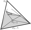
  (a)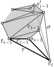

  

  (b)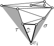

  

  (c)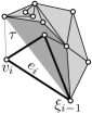

  

  (d)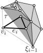

  

  (e)

  Figure 28: Embedding $\mathcal{C}_{i}$ (thick black) together with $\Gamma^{i-1}_{1}$. (a) In order to establish whether $\Gamma^{i-1}_{1}$ (whose convex hull is gray) fits inside $\mathcal{C}_{i}$, the slopes of the edges of $\mathcal{C}_{i}$ incident to $v_{i}$ are compared with the slopes of the segments of $\mathcal{B}^{i-1}_{1}$ incident to the end-vertices of $e_{i-1}$ and different from $e_{i-1}$ (lines through these segments are dark gray). (b) If $\mathcal{C}_{i}$ is embedded so that $v_{i-1}$ and $v_{i}$ lie on different sides of the line through $e_{i-1}$, then $\mathcal{B}^{i}_{1}$ has to be computed; Melkman’s algorithm [37] examines the segments from $v_{i}$ to the vertices that follow $s_{i-1}$ in counter-clockwise order along $\mathcal{B}^{i-1}_{1}$, until it finds a segment (dark gray) from $v_{i}$ to a vertex $s^{\prime}_{i-1}$ that keeps the previously encountered segment $\sigma$ to the right. (c) If $e_{i}$ lies in the interior of the convex hull of $\Gamma^{i}_{1}$, except possibly for its end-vertices, then the segments $\sigma$ and $\tau$ of $\mathcal{B}^{i}_{1}$ incident to $\xi_{i}=v_{i}$ represent the only “way out” of $\mathcal{B}^{i}_{1}$ for a planar straight-line realization of $G^{x-1}_{1}$; in particular, in any $e_{x-1}$-outer realization of $G^{x-1}_{1}$, the vertices and edges that are not in $G^{i}_{1}$ and that lie inside $\mathcal{B}^{i}_{1}$ can only lie in the dark gray regions incident to $\sigma$ and $\tau$. (d) Illustration for the case in which $v_{i}$ lies outside the convex hull of $\Gamma^{i-1}_{1}$ and $\xi_{i-1}$ is the end-vertex of $e_{i}$ different from $v_{i}$. (e) Illustration for the case in which $v_{i}$ lies outside the convex hull of $\Gamma^{i-1}_{1}$ and $\xi_{i-1}$ is not the end-vertex of $e_{i}$ different from $v_{i}$.

  In order to compute $\mathcal{B}^{i}_{1}$ from $\mathcal{B}^{i-1}_{1}$, Melkman’s algorithm [37] works as follows; refer to Fig. 28(b). Let $s_{i-1}$ and $t_{i-1}$ be the end-vertices of $e_{i-1}$ and assume that $s_{i-1}$ immediately precedes $t_{i-1}$ in clockwise order along $\mathcal{B}^{i-1}_{1}$. Since $v_{i}$ is a vertex of $\mathcal{B}^{i}_{1}$, the algorithm needs to find the vertices of $\mathcal{B}^{i-1}_{1}$ that follow $v_{i}$ in clockwise and counter-clockwise order along $\mathcal{B}^{i}_{1}$. In order to find the vertex that follows $v_{i}$ in counter-clockwise order along $\mathcal{B}^{i}_{1}$ (the computation of the other vertex is done similarly), the algorithm computes the segments from $v_{i}$ to the vertices of $\mathcal{B}^{i-1}_{1}$, starting from $s_{i-1}$ and proceeding in counter-clockwise order along $\mathcal{B}^{i-1}_{1}$. This computation stops when a segment from $v_{i}$ to a vertex $s^{\prime}_{i-1}$ of $\mathcal{B}^{i-1}_{1}$ is considered such that the oriented line that passes first through $v_{i}$ and then through $s^{\prime}_{i-1}$ keeps the previously encountered segment $\sigma$ to the right. When that happens, the end-vertex of $\sigma$ different from $v_{i}$ is the vertex that follows $v_{i}$ in counter-clockwise order along $\mathcal{B}^{i}_{1}$. This computation does not, in general, take $O(1)$ time, however it takes linear time in the number of vertices of $\mathcal{B}^{i-1}_{1}$ that are not in $\mathcal{B}^{i}_{1}$, hence it takes $O(n)$ time over all the convex hull computations.

  Let $\sigma$ and $\tau$ be the segments of $\mathcal{B}^{i}_{1}$ incident to $v_{i}$. In order to compute $\beta(e_{i})$ and $\xi_{i}$, we check whether $e_{i}$ coincides with one of $\sigma$ and $\tau$. In the positive case, we let $\beta(e_{i})=\texttt{True}$ and $\xi_{i}=\texttt{Null}$. In the negative case, we let $\beta(e_{i})=\texttt{False}$ and $\xi_{i}=v_{i}$. We are now ready to explain the meaning of the information conveyed in $\xi_{i}$; refer to Fig. 28(c). If $e_{i}$ lies in the interior of the convex hull of $\Gamma^{i}_{1}$, except possibly for one of its end-vertices, then the segments $\sigma$ and $\tau$ of $\mathcal{B}^{i}_{1}$ incident to $\xi_{i}$ represent the only “way out” of $\mathcal{B}^{i}_{1}$ for a planar straight-line realization of $G^{x-1}_{1}$. Formally, let $j$ be the smallest index such that $j>i$ and such that $v_{j}$ lies outside $\mathcal{B}^{i}_{1}$ in a planar straight-line realization of $G^{j}_{1}$, if any such an index exists; then (at least) one of the two edges incident to $v_{j}$ in $G^{j}_{1}$ crosses $\sigma$ or $\tau$. This very same property is exploited in Melkman’s algorithm [37], and comes from the fact that, by the connectivity of $G^{i}_{1}$, any path that starts at $v_{i}$, that does not share any vertex with $G^{i}_{1}$ other than $v_{i}$, and that first intersects the interior of the convex hull of $\Gamma^{i}_{1}$ and then crosses $\mathcal{B}^{i}_{1}$ in a segment different from $\sigma$ and $\tau$ crosses $\Gamma^{i}_{1}$ as well.

Case 2: $\beta(e_{i-1})=\texttt{False}$. In this case $\Gamma^{i-1}_{1}$ lies on both sides of the line through $e_{i-1}$, hence $\Gamma^{i-1}_{1}$ and $\mathcal{C}_{i}$ cannot be combined in order to form a same-side $e_{i}$-outer realization of $G^{i}_{1}$, even if $\Gamma^{i-1}_{1}$ is planar. Thus, as in Case 1.2, we let $\Gamma^{i}_{1}$ be the straight-line realization obtained from $\Gamma^{i-1}_{1}$ by embedding $\mathcal{C}_{i}$ in such a way that $v_{i-1}$ and $v_{i}$ lie on different sides of the line through $e_{i-1}$; this is again the realization which was earlier called $\Gamma^{i,a}_{1}$. The plane embedding $\mathcal{E}(\Gamma^{i}_{1})$ is computed in $O(1)$ time from $\mathcal{E}(\Gamma^{i-1}_{1})$ as in Case 1.2. Then $\Gamma^{i}_{1}$ satisfies the invariant; indeed, in the description of the algorithm, it was proved that, if $\Gamma^{i,a}_{1}$ is planar, then it is $e_{i}$-optimal, otherwise $G^{i}_{1}$ admits no $e_{i}$-outer realization. Further, $\Gamma^{i}_{1}$ can be constructed in $O(1)$ time from $\Gamma^{i-1}_{1}$. Note that, in this case, it might happen that $\Gamma^{i}_{1}$ is not planar even if $\Gamma^{i-1}_{1}$ is planar; however, we do not check the planarity of $\Gamma^{i}_{1}$ at this time.

In order to compute $\mathcal{B}^{i}_{1}$, $\beta(e_{i})$, and $\xi_{i}$, we exploit the information stored in $\xi_{i-1}$. As explained in Case 1.2, if $\Gamma^{i-1}_{1}$ is planar, the value $\xi_{i-1}$ represents a vertex on the boundary $\mathcal{B}^{i-1}_{1}$ of the convex hull of $\Gamma^{i-1}_{1}$ such that $v_{i}$ lies outside $\mathcal{B}^{i-1}_{1}$ only if the (at least one) edge $e$ of $c_{i}$ incident to $v_{i}$ and not incident to $\xi_{i-1}$ crosses $\sigma$ or $\tau$, where $\sigma$ and $\tau$ are the segments incident to $\xi_{i-1}$ in $\mathcal{B}^{i-1}_{1}$. Hence, we (as in Melkman’s algorithm [37]) check in $O(1)$ time whether $e$ crosses $\sigma$ or $\tau$.

• In the positive case, $v_{i}$ lies outside the convex hull of $\Gamma^{i-1}_{1}$; then $\mathcal{B}^{i}_{1}$ is constructed as in Case 1.2, where the segment between $\sigma$ and $\tau$ that crosses $e$ plays the role of $e_{i-1}$. If $\xi_{i-1}$ is the end-vertex of $e_{i}$ different from $v_{i}$, as in Fig. 28(d), then we set $\beta(e_{i})=\texttt{True}$ and $\xi_{i}=\texttt{Null}$ (in this case $G^{i}_{1}$ “made it out” of $\mathcal{B}^{i-1}_{1}$), otherwise, as in Fig. 28(e), we set $\beta(e_{i})=\texttt{False}$ and $\xi_{i}=v_{i}$.

• In the negative case, $v_{i}$ lies inside the convex hull of $\Gamma^{i-1}_{1}$ or $\Gamma^{i}_{1}$ is not planar (or both). Hence, we set $\mathcal{B}^{i}_{1}=\mathcal{B}^{i-1}_{1}$, $\beta(e_{i})=\texttt{False}$, and $\xi_{i}=\xi_{i-1}$.

This concludes the description of the inductive case of our algorithm. Each inductive step takes $O(1)$ time, except for the computation of the boundaries $\mathcal{B}^{1}_{1},\mathcal{B}^{2}_{1},\dots,\mathcal{B}^{x-1}_{1}$, which however takes total $O(n)$ time as explained above. Hence, the overall running time of the algorithm is in $O(n)$. ∎

Figure 29: The outerplane embedding of an outerpillar. The gray face is the one bounded by $c_{x}$. The graphs $G_{1}$ and $G_{2}$ are enclosed inside fat curves.

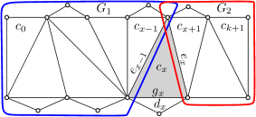
Proof of Theorem 6.2. The proof uses several ideas from the proof of Theorem 6.1. We hence omit details of arguments that have been already detailed in that proof.

Let $G=(V,E,\lambda)$ be an $n$-vertex weighted maximal outerpillar (as the one in Fig. 29) and let $\mathcal{O}$ be its outerplane embedding, which can be found in $O(n)$ time [21, 38, 50]. Since $G$ is an outerpillar, its dual tree is a caterpillar $T$, whose spine we denote by $P:=(p_{1},\dots,p_{k})$; note that $T$ can be easily recovered from $\mathcal{O}$ in $O(n)$ time. We arbitrarily select two leaves of $T$, respectively adjacent to $p_{1}$ and $p_{k}$, and denote them by $p_{0}$ and $p_{k+1}$; we further denote by $\overline{P}$ the path $(p_{0},p_{1},\dots,p_{k},p_{k+1})$. Each node $p_{i}$ of $\overline{P}$ corresponds to an internal face of $\mathcal{O}$; we denote by $c_{i}$ the $3$-cycle of $G$ bounding such a face. Further, each node $p_{i}$ in $\overline{P}$ is adjacent to at most one leaf not in $\overline{P}$ (the satisfaction of this property was the reason to augment $P$ to $\overline{P}$), which corresponds to an internal face of $\mathcal{O}$; we denote by $d_{i}$ the $3$-cycle of $G$ bounding such a face. Each cycle $c_{i}$ has a unique (planar) straight-line realization (up to a rigid transformation), which we denote by $\mathcal{C}_{i}$, and each cycle $d_{i}$ has a unique (planar) straight-line realization (up to a rigid transformation), which we denote by $\mathcal{D}_{i}$. For $i=0,\dots,k$, let $e_{i}$ be the edge of $G$ that is dual to the edge $(p_{i},p_{i+1})$ of $\overline{P}$; note that $e_{i}$ is an internal edge of $\mathcal{O}$. Further, for every index $i\in\{1,\dots,k\}$ such that $d_{i}$ exists, let $g_{i}$ be the edge shared by $c_{i}$ and $d_{i}$.

Let $c^{*}$ be a $3$-cycle of $G$ whose edges have a sum of the lengths which is maximum among all the $3$-cycles of $G$. Let $x\in\{0,1,\dots,k+1\}$ be the index such that we have either $c^{*}=c_{x}$ or $c^{*}=d_{x}$. Let $G_{1}$ be the subgraph of $G$ composed of the $3$-cycles $c_{i}$ and of the $3$-cycles $d_{i}$ with $i=0,\dots,x-1$ (some of the $3$-cycles $d_{i}$ might not exist). Analogously, let $G_{2}$ be the subgraph of $G$ composed of the $3$-cycles $c_{i}$ and of the $3$-cycles $d_{i}$ with $i=x+1,\dots,k+1$ (again, some of the $3$-cycles $d_{i}$ might not exist). One of these graphs might be undefined if $x=0$ or $x=k+1$; however, in the following, we assume that $1\leq x\leq k$ as the arguments for the cases $x=0$ and $x=k+1$ are analogous and actually simpler. Note that $G_{1}$ and $G_{2}$ are maximal outerpillars. Also, we assume that the $3$-cycle $d_{x}$ exists, as the argument for the case in which it does not is simpler.

Assume that a planar straight-line realization $\Gamma$ of $G$ exists; for $i=1,2$, let $\Gamma_{i}$ be the restriction of $\Gamma$ to $G_{i}$. If $c^{*}=c_{x}$, then $c_{x}$ does not lie inside any $3$-cycle of $G$ in $\Gamma$. If $c^{*}=d_{x}$, then $c_{x}$ might lie inside $d_{x}$ in $\Gamma$, however it does not lie inside any other $3$-cycle of $G$ in $\Gamma$, as otherwise, by planarity, such a $3$-cycle would also contain $d_{x}$, which is not possible. Therefore, both if $c^{*}=c_{x}$ and if $c^{*}=d_{x}$, we have that $\Gamma_{1}$ is an $e_{x-1}$-outer realization of $G_{1}$ and that $\Gamma_{2}$ is an $e_{x}$-outer realization of $G_{2}$.

We show an $O(n^{3})$-time algorithm that either concludes that $G_{1}$ admits no $e_{x-1}$-outer realization or constructs an $e_{x-1}$-optimal set $\mathcal{R}_{1}$ of $e_{x-1}$-outer realizations of $G_{1}$, where for each realization $\Gamma_{1}$ in $\mathcal{R}_{1}$ the plane embedding $\mathcal{E}(\Gamma_{1})$ is constructed as well. The same algorithm is then also used in order to either conclude that $G_{2}$ admits no $e_{x}$-outer realization or to construct an $e_{x}$-optimal set $\mathcal{R}_{2}$ of $e_{x}$-outer realizations of $G_{2}$, where for each realization $\Gamma_{2}$ in $\mathcal{R}_{2}$ the plane embedding $\mathcal{E}(\Gamma_{2})$ is constructed as well.

For $i=0,1,\dots,x-1$, let $G^{i}_{1}$ be the subgraph of $G_{1}$ composed of the $3$-cycles $c_{0},c_{1},\dots,c_{i}$ and of the $3$-cycles $d_{0},d_{1},\dots,d_{i}$ (some of these $3$-cycles might not exist); note that $G^{x-1}_{1}=G_{1}$. As in the proof of Theorem 6.1, we use the observation that the restriction of any $e_{x-1}$-outer realization of $G_{1}$ to $G^{i}_{1}$ is an $e_{i}$-outer realization of $G^{i}_{1}$.

Our algorithm works by induction on $i$ in order to either conclude that $G^{i}_{1}$ admits no $e_{i}$-outer realization (and thus $G_{1}$ admits no $e_{x-1}$-outer realization), or to determine an $e_{i}$-optimal set $\mathcal{R}^{i}_{1}$ of $e_{i}$-outer realizations of $G^{i}_{1}$ with $|\mathcal{R}^{i}_{1}|\leq i+1$, where for each realization $\Gamma^{i}_{1}$ in $\mathcal{R}^{i}_{1}$ the plane $\mathcal{E}(\Gamma^{i}_{1})$ is constructed as well. This is trivial when $i=0$, namely $G^{0}_{1}$ is the $3$-cycle $c_{0}$ which has a unique planar straight-line realization $\Gamma^{0}_{1}:=\mathcal{C}_{0}$, up to a rigid transformation; then $\mathcal{R}^{0}_{1}:=\{\Gamma^{0}_{1}\}$ is indeed an $e_{0}$-optimal set of $e_{0}$-outer realizations of $G^{0}_{1}$ with $|\mathcal{R}^{0}_{1}|\leq 1$ and $\mathcal{E}(\Gamma^{0}_{1})$ is easily computed from $\Gamma^{0}_{1}$.

Assume that we have an $e_{i-1}$-optimal set $\mathcal{R}^{i-1}_{1}$ of $e_{i-1}$-outer realizations of $G^{i-1}_{1}$ with $|\mathcal{R}^{i-1}_{1}|\leq i$, for some $i\in\{1,\dots,x-1\}$, and we have, for each realization $\Gamma^{i-1}_{1}$ in $\mathcal{R}^{i-1}_{1}$, the plane embedding $\mathcal{E}(\Gamma^{i-1}_{1})$; indeed, if we already concluded that $G_{1}$ admits no $e_{x-1}$-outer realization, there is nothing else to do. We present an algorithm that either concludes that $G_{1}$ admits no $e_{x-1}$-outer realization or constructs the set $\mathcal{R}^{i}_{1}$ and, for each realization $\Gamma^{i}_{1}$ in $\mathcal{R}^{i}_{1}$, the plane embedding $\mathcal{E}(\Gamma^{i}_{1})$. The algorithm consists of three steps.

• Step 1. In the first step, we aim for the construction of an $e_{i}$-outer realization of $G^{i}_{1}$ in which both $G^{i-1}_{1}$ and $d_{i}$ lie inside $c_{i}$ (except for the edges $e_{i-1}$ and $g_{i}$, which $c_{i}$ shares with $G^{i-1}_{1}$ and $d_{i}$, respectively), as the one in Fig. 30(a). This is done by checking whether any of the $O(n)$ realizations of $G^{i-1}_{1}$ in $\mathcal{R}^{i-1}_{1}$ fits inside $\mathcal{C}_{i}$ together with $\mathcal{D}_{i}$. More precisely, we act as follows.

  1. We test in $O(1)$ time whether $\mathcal{C}_{i-1}$ lies inside $\mathcal{C}_{i}$ once they coincide on the representation of $e_{i-1}$ and once their vertices not incident to $e_{i-1}$ lie on the same side of the line through $e_{i-1}$. If the test is positive, we proceed with the first step of the algorithm, otherwise we conclude that no realization of $G^{i-1}_{1}$ fits inside $\mathcal{C}_{i}$, we terminate the first step of the algorithm and proceed to the second one.

  2. We test in $O(1)$ time whether $\mathcal{D}_{i}$ lies inside $\mathcal{C}_{i}$ once they coincide on the representation of $g_{i}$ and once their vertices not incident to $g_{i}$ lie on the same side of the line through $g_{i}$; if $d_{i}$ does not exist, this test is skipped. If the test is positive, we proceed with the first step of the algorithm, otherwise we conclude that $\mathcal{D}_{i}$ does not fit inside $\mathcal{C}_{i}$, we terminate the first step of the algorithm and proceed to the second one.

  3. For each realization $\Gamma^{i-1}_{1}$ of $G^{i-1}_{1}$ in $\mathcal{R}^{i-1}_{1}$, we construct a straight-line realization $\Gamma^{i}_{1}$ of $G^{i}_{1}$ in which $G^{i-1}_{1}$ is represented by $\Gamma^{i-1}_{1}$ and $\mathcal{C}_{i-1}$ and $\mathcal{D}_{i}$ are embedded inside $\mathcal{C}_{i}$. Such a realization can be obtained in $O(1)$ time by augmenting $\Gamma^{i-1}_{1}$ with a representation of the edges of $c_{i}$ and $d_{i}$ not in $G^{i-1}_{1}$. Further, the plane embedding $\mathcal{E}(\Gamma^{i}_{1})$ can be constructed in $O(1)$ time by inserting the edges incident to $v_{i}$ next to $e_{i-1}$ in the cyclic order of the edges incident to the end-vertices of $e_{i-1}$, by then inserting the edges of $d_{i}$ different from $g_{i}$ next to $g_{i}$ in the cyclic order of the edges incident to the end-vertices of $g_{i}$, and by letting the outer face of $\mathcal{E}(\Gamma^{i}_{1})$ be bounded by the cycle $c_{i}$. We then test in $O(n)$ time, by means of Theorem 3.1, whether $\Gamma^{i}_{1}$ is a planar straight-line realization of $G^{i}_{1}$ respecting $\mathcal{E}(\Gamma^{i}_{1})$.

  

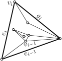
  (a)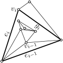

  

  (b)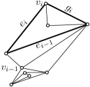

  

  (c)

  Figure 30: Three $e_{i}$-outer realizations of $G^{i}_{1}$. The cycle $c_{i}$ is represented by a thick line. (a) $G^{i-1}_{1}$ and $d_{i}$ lie inside $c_{i}$; (b) $G^{i-1}_{1}$ lies inside $c_{i}$ and $d_{i}$ lies outside $c_{i}$; (c) $G^{i-1}_{1}$ lies outside $c_{i}$.

  The total running time of the first step of the algorithm is hence in $O(n^{2})$. If (at least) one of these tests succeeds in constructing a realization $\Gamma^{i}_{1}$, then we complete the induction with $\mathcal{R}^{i}_{1}=\{\Gamma^{i}_{1}\}$. If none of the tests succeeds, we proceed to the second step of the algorithm.

• Step 2. In the second step, we aim for the construction of an $e_{i}$-outer realization of $G^{i}_{1}$ in which $G^{i-1}_{1}$ lies inside $c_{i}$ (except for the edge $e_{i-1}$, which is shared by $G^{i-1}_{1}$ and $c_{i}$) and $d_{i}$ lies outside $c_{i}$ (except for the edge $g_{i}$, which is shared by $c_{i}$ and $d_{i}$), as in Fig. 30(b). If $d_{i}$ does not exist, then this step is actually ignored, given that the desired representation of $G^{i}_{1}$ would have been already constructed in the first step. As in the first step, we first check whether $\mathcal{C}_{i-1}$ lies inside $\mathcal{C}_{i}$ once they coincide on the representation of $e_{i-1}$ and once their vertices not incident to $e_{i-1}$ lie on the same side of the line through $e_{i-1}$. If the test is negative, we conclude that no realization of $G^{i-1}_{1}$ fits inside $\mathcal{C}_{i}$, we terminate the second step of the algorithm and proceed to the third one with $\mathcal{R}^{i}_{1}=\emptyset$. If the test is positive, we independently consider each of the $O(n)$ realizations of $G^{i-1}_{1}$ in $\mathcal{R}^{i-1}_{1}$, say $\Gamma^{i-1}_{1}$. We augment $\Gamma^{i-1}_{1}$ to a realization $\Gamma^{i}_{1}$ of $G^{i}_{1}$ (and compute the plane embedding $\mathcal{E}(\Gamma^{i}_{1})$ from the plane embedding $\mathcal{E}(\Gamma^{i-1}_{1})$) in $O(1)$ time similarly as in the first step, except that $\mathcal{D}_{i}$ is now embedded outside $\mathcal{C}_{i}$ and hence the outer face of $\mathcal{E}(\Gamma^{i}_{1})$ is now delimited by the edges of $c_{i}$ and $d_{i}$ different from $g_{i}$. By means of Theorem 3.1, we test in $O(n)$ time whether $\Gamma^{i}_{1}$ is a planar straight-line realization of $G^{i}_{1}$ respecting $\mathcal{E}(\Gamma^{i}_{1})$. Hence, the total running time of the second step is in $O(n^{2})$. If (at least) one of these tests shows that a realization $\Gamma^{i}_{1}$ of $G^{i}_{1}$ is planar, we conclude this step by initializing $\mathcal{R}^{i}_{1}=\{\Gamma^{i}_{1}\}$. If none of the tests succeeds, then we initialize $\mathcal{R}^{i}_{1}=\emptyset$. In both cases, we proceed to the third step of the algorithm.

• Step 3. In the third step, we aim for the construction of (possibly multiple) $e_{i}$-outer realizations of $G^{i}_{1}$ in which $G^{i-1}_{1}$ lies outside $c_{i}$ (except for the edge $e_{i-1}$, which is shared by $G^{i-1}_{1}$ and $c_{i}$), as in Fig. 30(c). This is done as follows. Preliminarly, we construct a realization of $c_{i}\cup d_{i}$ (if $d_{i}$ exists). In order to do that, we check in $O(1)$ time whether $\mathcal{D}_{i}$ fits inside $\mathcal{C}_{i}$; in the positive case, we place it inside $\mathcal{C}_{i}$, otherwise we place it outside $\mathcal{C}_{i}$. We now independently consider each $e_{i-1}$-outer realization $\Gamma^{i-1}_{1}$ of $G^{i-1}_{1}$ in $\mathcal{R}^{i-1}_{1}$ and we put it together with the constructed representation of $c_{i}\cup d_{i}$ (if $d_{i}$ does not exist, we just put $\Gamma^{i-1}_{1}$ together with $\mathcal{C}_{i}$), so that the vertices of $c_{i-1}$ and $c_{i}$ not incident to $e_{i-1}$ lie on different sides of the line through $e_{i-1}$. This can be done in $O(1)$ time, as in the first and second steps, by augmenting $\Gamma^{i-1}_{1}$ with a representation of the edges of $c_{i}$ and $d_{i}$ not in $G^{i-1}_{1}$. The plane embedding of the constructed representation of $G^{i}_{1}$ can also be constructed in $O(1)$ time from the plane embedding $\mathcal{E}(\Gamma^{i-1}_{1})$, similarly as in the first and second steps. We now check in $O(n)$ time whether the constructed representation of $G^{i}_{1}$ is a planar straight-line realization of $G^{i}_{1}$ respecting the constructed plane embedding, by means of Theorem 3.1; in the positive case, we add it to $\mathcal{R}^{i}_{1}$. Hence, the total running time of the third step is in $O(n^{2})$. After the third step, if $\mathcal{R}^{i}_{1}=\emptyset$, we conclude that $G_{1}$ admits no $e_{x-1}$-outer realization.

This concludes the description of the algorithm. We now prove its correctness.

First, we prove that $|\mathcal{R}^{i}_{1}|\leq i+1$. This is obvious if the first step succeeded in the construction of a realization of $G^{i}_{1}$, as in that case we have $|\mathcal{R}^{i}_{1}|=1<i+1$. Otherwise, at most one realization of $G^{i}_{1}$ was added to $\mathcal{R}^{i}_{1}$ in the second step; further, during the third step, at most one realization of $G^{i}_{1}$ was added to $\mathcal{R}^{i}_{1}$ for each realization in $\mathcal{R}^{i-1}_{1}$. Since $|\mathcal{R}^{i-1}_{1}|\leq i$, by the inductive hypothesis, it follows that $|\mathcal{R}^{i}_{1}|\leq i+1$.

Second, we have that each realization in $\mathcal{R}^{i}_{1}$ is planar, as ensured by a test performed on it before the insertion into $\mathcal{R}^{i}_{1}$. Further, each realization in $\mathcal{R}^{i}_{1}$ is $e_{i}$-outer. Namely, if the vertices of $c_{i-1}$ and $c_{i}$ that are not incident to $e_{i-1}$ lie on the same side of the line through $e_{i-1}$, we test whether $\mathcal{C}_{i-1}$ lies inside $\mathcal{C}_{i}$; further, if the vertices of $d_{i}$ and $c_{i}$ that are not incident to $g_{i}$ lie on the same side of the line through $g_{i}$, we test whether $\mathcal{D}_{i}$ lies inside $\mathcal{C}_{i}$. A realization is added to $\mathcal{R}^{i}_{1}$ only if both tests succeed, which ensures that $\mathcal{C}_{i}$ does not lie inside $\mathcal{C}_{i-1}$ or $\mathcal{D}_{i}$ in any realization in $\mathcal{R}^{i}_{1}$. A containment of $\mathcal{C}_{i}$ inside any other $3$-cycle of $G^{i}_{1}$ would contradict the planarity of the corresponding realization.

Finally, we prove that $\mathcal{R}^{i}_{1}$ is $e_{i}$-optimal. This can be done very similarly as in the proof of Theorem 6.1. Namely, consider any $e_{i}$-outer realization $\Psi^{i}_{1}$ of $G^{i}_{1}$ and let $\Psi^{i-1}_{1}$ be the restriction of $\Psi^{i}_{1}$ to $G^{i-1}_{1}$. Since $\mathcal{R}^{i-1}_{1}$ is $e_{i-1}$-optimal, there exists an $e_{i-1}$-outer realization $\Lambda^{i-1}_{1}$ of $G^{i-1}_{1}$ in $\mathcal{R}^{i-1}_{1}$ such that $\Lambda^{i-1}_{1}$ is $e_{i-1}$-smaller than $\Psi^{i-1}_{1}$. Hence, we can apply Lemma 21 with $H=G^{i-1}_{1}$, $K=c_{i}\cup d_{i}$ (or $K=c_{i}$ if $d_{i}$ does not exist), $\mathcal{G}=\Psi^{i}_{1}$, $e=e_{i-1}$, and $\mathcal{H}^{\prime}=\Lambda^{i-1}_{1}$, in order to obtain an $e_{i}$-outer realization $\Lambda^{i}_{1}$ of $G^{i}_{1}$ whose restriction to $G^{i-1}_{1}$ can be obtained by a rigid transformation of $\Lambda^{i-1}_{1}$ and such that $\mathcal{C}_{i-1}$ lies inside $\mathcal{C}_{i}$ in $\Lambda^{i}_{1}$ if and only if $\mathcal{C}_{i-1}$ lies inside $\mathcal{C}_{i}$ in $\Psi^{i}_{1}$. It only remains to prove that $\Lambda^{i}_{1}$, or an $e_{i}$-outer realization that is $e_{i}$-smaller than $\Lambda^{i}_{1}$, actually belongs to $\mathcal{R}^{i}_{1}$.

First, if $\mathcal{R}^{i}_{1}$ contains a single realization $\Gamma^{i}_{1}$ added during the first step, then the outer face of $\Gamma^{i}_{1}$ is bounded by $\mathcal{C}_{i}$; since the set $\mathcal{I}_{\Lambda^{i}_{1}}$ contains at least the closure of the interior of $\mathcal{C}_{i}$, we have that $\Gamma^{i}_{1}$ is $e_{i}$-smaller than $\Lambda^{i}_{1}$. We can hence assume that $\Lambda^{i-1}_{1}$ lies outside $\mathcal{C}_{i}$ or that $\mathcal{D}_{i}$ lies outside $\mathcal{C}_{i}$ (or both). Indeed, if both $\Lambda^{i-1}_{1}$ and $\mathcal{D}_{i}$ lied inside $\mathcal{C}_{i}$, then the first step of the algorithm would have constructed $\Lambda^{i}_{1}$, and hence $\mathcal{R}^{i}_{1}$ would contain a single realization $\Gamma^{i}_{1}$ added during the first step (note that $\Gamma^{i}_{1}$ would not necessarily be the same as $\Lambda^{i}_{1}$, however the outer faces of both $\Gamma^{i}_{1}$ and $\Lambda^{i}_{1}$ would be delimited by $\mathcal{C}_{i}$).

Second, consider the case in which $\Lambda^{i-1}_{1}$ lies inside $\mathcal{C}_{i}$ and $\mathcal{D}_{i}$ lies outside $\mathcal{C}_{i}$ in $\Lambda^{i}_{1}$. This implies that the second step of the algorithm constructs $\Lambda^{i}_{1}$, and hence $\mathcal{R}^{i}_{1}$ contains a realization $\Gamma^{i}_{1}$ added during the second step of the algorithm. The outer face of $\Gamma^{i}_{1}$ is bounded by the edges of $\mathcal{C}_{i}$ and $\mathcal{D}_{i}$ different from $g_{i}$, same as $\Lambda^{i}_{1}$, hence $\Gamma^{i}_{1}$ is $e_{i}$-smaller than $\Lambda^{i}_{1}$.

Third, consider the case in which $\Lambda^{i-1}_{1}$ lies outside $\mathcal{C}_{i}$. If $\mathcal{D}_{i}$ lies inside $\mathcal{C}_{i}$ in $\Lambda^{i}_{1}$, or if $\mathcal{D}_{i}$ lies outside $\mathcal{C}_{i}$ in $\Lambda^{i}_{1}$ and does not fit inside $\mathcal{C}_{i}$, then the third step of the algorithm constructs $\Lambda^{i}_{1}$ and adds it to $\mathcal{R}^{i}_{1}$. If $\mathcal{D}_{i}$ lies outside $\mathcal{C}_{i}$ in $\Lambda^{i}_{1}$ and fits inside $\mathcal{C}_{i}$, then the third step of the algorithm constructs a realization $\Gamma^{i}_{1}$ which coincides with $\Lambda^{i}_{1}$ when restricted to $G^{i-1}_{1}\cup c_{i}$, but in which $\mathcal{D}_{i}$ lies inside $\mathcal{C}_{i}$. Then we have that $\Gamma^{i}_{1}$ is $e_{i}$-smaller than $\Lambda^{i}_{1}$. This concludes the proof of the $e_{i}$-optimality of $\mathcal{R}^{i}_{1}$ and of the correctness of the inductive step.

The inductive step is hence performed in $O(n^{2})$ time. Since there are $O(n)$ inductive steps, our algorithm takes $O(n^{3})$ time in order to either conclude that $G_{1}$ admits no $e_{x-1}$-outer realization or to construct an $e_{x-1}$-optimal set $\mathcal{R}_{1}$ with $|\mathcal{R}_{1}|\in O(n)$ of $e_{x-1}$-outer realizations of $G_{1}$ together with the plane embedding $\mathcal{E}(\Gamma_{1})$ of each realization $\Gamma_{1}$ in $\mathcal{R}_{1}$; the algorithm also takes $O(n^{3})$ time in order to either conclude that $G_{2}$ admits no $e_{x}$-outer realization or to construct an $e_{x}$-optimal set $\mathcal{R}_{2}$ with $|\mathcal{R}_{2}|\in O(n)$ of $e_{x}$-outer realizations of $G_{2}$ together with the plane embedding $\mathcal{E}(\Gamma_{2})$ of each realization $\Gamma_{2}$ in $\mathcal{R}_{2}$.

As argued above, if $G_{1}$ admits no $e_{x-1}$-outer realization or $G_{2}$ admits no $e_{x}$-outer realization, then $G$ admits no planar straight-line realization. Assume hence that $\mathcal{R}_{1}$ and $\mathcal{R}_{2}$ are both non-empty. We independently consider each pair $(\Gamma_{1},\Gamma_{2})$ such that $\Gamma_{1}\in\mathcal{R}_{1}$ and $\Gamma_{2}\in\mathcal{R}_{2}$; since $|\mathcal{R}_{1}|$ and $|\mathcal{R}_{2}|$ are both in $O(n)$, there are $O(n^{2})$ such pairs. We construct eight straight-line realizations of $G$, each with the corresponding plane embedding, according to the following choices:

• the vertices of $c_{x-1}$ and $c_{x}$ not incident to $e_{x-1}$ might lie on the same side or on different sides of the line through $e_{x-1}$;

• the vertices of $c_{x+1}$ and $c_{x}$ not incident to $e_{x}$ might lie on the same side or on different sides of the line through $e_{x}$; and

• the vertices of $d_{x}$ and $c_{x}$ not incident to $g_{x}$ might lie on the same side or on different sides of the line through $g_{x}$.

We test in $O(n)$ time whether each of these straight-line realizations is planar and respects the corresponding plane embedding, by means of Theorem 3.1. Hence, all these tests can be performed in overall $O(n^{3})$ time. If (at least) one of these realizations is planar, then it is the desired planar straight-line realization of $G$. Otherwise, there exists no planar straight-line realization of $G$; this can be proved as in the proof of Theorem 6.1. Namely, if a planar straight-line realization $\Gamma$ of $G$ exists, then the restriction of $\Gamma$ to $G_{1}$ and the restriction of $\Gamma$ to $G_{2}$ can be replaced by straight-line realizations obtained by rigid transformations of suitable realizations in $\mathcal{R}_{1}$ and $\mathcal{R}_{2}$, respectively. By Lemma 21, this results in a planar straight-line realization of $G$ which, by construction, is one of the straight-line realizations for which the planarity testing was negative. This contradiction concludes the proof of the theorem. ∎

7 2-Trees with Short Longest Path

In this section, we show that the FEPR problem is polynomial-time solvable for weighted $2$-trees whose longest path has bounded length, where the length of a path is the number of edges in it. Our algorithm actually runs in polynomial time in a more general case: if the height of the SPQ-tree of the $2$-tree is bounded. We start this section by introducing the necessary definitions and notation.

The notion of SPQ-tree is a specialization of the well-known notion of SPQR-tree [24, 31] for series-parallel graphs [23, 49]. A series-parallel graph is any graph that can be obtained by means of the following recursive construction (see Fig. 31).

Figure 31: A $2$-tree $G$ and its SPQ-tree $\mathcal{T}$. The gray regions show $G_{\mu}$ and $\mathcal{T}_{\mu}$, for a node $\mu$ of $\mathcal{T}$. The poles of $\mu$ are represented by empty disks in $G$. The fat edge corresponds to the Q-node that is a child of the root of $\mathcal{T}$. The height of $\mathcal{T}$ is $8$, the one of $\mathcal{T}_{\mu}$ is $4$.

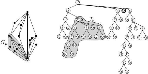
• An edge $(u,v)$ is a series-parallel graph with two poles $u$ and $v$; its SPQ-tree $\mathcal{T}$ is rooted tree with a single Q-node. We say that $(u,v)$ corresponds to the Q-node (and vice versa).

• Let $G_{1},\dots,G_{k}$ be series-parallel graphs, where $G_{i}$ has poles $u_{i}$ and $v_{i}$, for $i=1,\dots,k$; also, let $\mathcal{T}_{1},\dots,\mathcal{T}_{k}$ be their SPQ-trees. The graph obtained by identifying the vertices $u_{1},\dots,u_{k}$ into a single vertex $u$ and the vertices $v_{1},\dots,v_{k}$ into a single vertex $v$ is a series-parallel graph $G$ with poles $u$ and $v$. The SPQ-tree $\mathcal{T}$ of $G$ is the tree whose root is a P-node which is the parent of the roots of $\mathcal{T}_{1},\dots,\mathcal{T}_{k}$. We say that $G$ corresponds to $\mathcal{T}$.

• Let $G_{1},\dots,G_{k}$ be series-parallel graphs, where $G_{i}$ has poles $u_{i}$ and $v_{i}$, for $i=1,\dots,k$; also, let $\mathcal{T}_{1},\dots,\mathcal{T}_{k}$ be their SPQ-trees. The graph obtained by identifying the vertex $v_{i}$ with the vertex $u_{i+1}$, for $i=1,\dots,k-1$, is a series-parallel graph $G$ with poles $u_{1}$ and $v_{k}$. The SPQ-tree $\mathcal{T}$ of $G$ is the tree whose root is an S-node which is the parent of the roots of $\mathcal{T}_{1},\dots,\mathcal{T}_{k}$. We say that $G$ corresponds to $\mathcal{T}$.

Every $2$-tree $G$ is a series-parallel graph (see, e.g., [13, Chapter 5]) such that:

1. The root of the SPQ-tree $\mathcal{T}$ of $G$ is a P-node.

2. Each P-node has at least two children; one of them is a Q-node and the others are S-nodes.

3. Each S-node has exactly two children, each of which is either a Q-node or a P-node.

Moreover, if $e$ is a prescribed edge of $G$, then the SPQ-tree of $G$ can be constructed in such a way that the Q-node corresponding to $e$ is a child of the root $\rho$ of the SPQ-tree (that is, $e$ is the edge between the poles of $\rho$). We will use this property later.

Let $G$ be a $2$-tree, $\mathcal{T}$ be the SPQ-tree of $G$, and $\mu$ be a node of $\mathcal{T}$. We denote by $u_{\mu}$ and $v_{\mu}$ the poles of $\mu$, by $\mathcal{T}_{\mu}$ the subtree of $\mathcal{T}$ rooted at $\mu$, and by $G_{\mu}$ the subgraph of $G$ corresponding to $\mathcal{T}_{\mu}$. The height of $\mathcal{T}$ is the maximum number of edges in any root-to-leaf path in $\mathcal{T}$. By Conditions (C1)–(C2), the height of $\mathcal{T}$ is even and positive.

We can upper bound the height of an SPQ-tree of a $2$-tree $G$ in terms of the length of the longest path of $G$, as proved in the following lemma.

Lemma 22.

Let $G$ be a $2$-tree, let $\ell$ be the length of the longest path of $G$, let $\mathcal{T}$ be the SPQ-tree of $G$, and let $h$ be the height of $\mathcal{T}$. Then we have $h\leq 2\ell-2$.

Proof.

We prove the following claim. For every P-node $\mu$ in $\mathcal{T}$, there exists a path $P_{\mu}$ in $G_{\mu}$ that connects the poles $u$ and $v$ of $\mu$ and whose length is $\frac{h_{\mu}}{2}+1$, where $h_{\mu}$ is the height of $\mathcal{T}_{\mu}$. The claim implies the lemma by choosing $\mu$ to be the root of $\mathcal{T}$; this can be done since, by Condition (C1), the root of $\mathcal{T}$ is a P-node.

We prove the claim by induction on $h_{\mu}$. Recall that $h_{\mu}$ is even and positive. Let $\nu$ be a child of $\mu$ such that the height of $\mathcal{T}_{\nu}$ is $h_{\mu}-1$; by Condition (C2) and since $h_{\mu}\geq 2$, we have that $\nu$ is an S-node with poles $u$ and $v$. By Condition (C3), we have that $\nu$ has two children $\nu_{1}$ and $\nu_{2}$, each of which is either a P-node or a Q-node. Assume, w.l.o.g. up to a relabeling, that $u$ is a pole of $\nu_{1}$, that $v$ is a pole of $\nu_{2}$, and that $w$ is the pole shared by $\nu_{1}$ and $\nu_{2}$.

In the base case, we have $h_{\mu}=2$. Then $\nu_{1}$ and $\nu_{2}$ are both Q-nodes, as otherwise the height of $\mathcal{T}$ would be greater than $2$. It follows that $G$ contains the path $P_{\mu}=(u,w,v)$.

In the inductive case, we have $h_{\mu}>2$. Assume that the height of $\mathcal{T}_{\nu_{1}}$ is $h_{\mu}-2$, as the case in which the height of $\mathcal{T}_{\nu_{2}}$ is $h_{\mu}-2$ is analogous. Since $h_{\mu}>2$, we have that $\nu_{1}$ is a P-node. By induction, $G_{\nu_{1}}$ contains a path $\mathcal{P}_{\nu_{1}}$ with length $\frac{h_{\mu}-2}{2}+1$ between $u$ and $w$. Further, $G_{\nu_{2}}$ contains the edge $(w,v)$; this is obvious if $\nu_{2}$ is a Q-node and comes from Condition (C2) otherwise. The path $\mathcal{P}_{\nu_{1}}\cup(w,v)$ is the desired path $\mathcal{P}_{\mu}$ with length $\frac{h_{\mu}}{2}+1$ between $u$ and $v$. This completes the induction and hence the proof of the lemma. ∎

The main result of this section is the following.

Theorem 7.1.

Let $G$ an $n$-vertex weighted $2$-tree, let $e^{*}$ be an edge of $G$ with maximum length, let $\mathcal{T}$ be the SPQ-tree of $G$ such that the Q-node corresponding to $e^{*}$ is a child of the root of $\mathcal{T}$, and let $h^{*}$ be the height of $\mathcal{T}$. There exists an $n^{O(2^{h^{*}})}$-time algorithm that tests whether $G$ admits a planar straight-line realization and, in the positive case, constructs such a realization.

Due to Lemma 22, Theorem 7.1 implies the following.

Corollary 1.

Let $G$ an $n$-vertex weighted $2$-tree and let $\ell$ be length of the longest path of $G$. There exists an $n^{O(4^{\ell})}$-time algorithm that tests whether $G$ admits a planar straight-line realization and, in the positive case, constructs such a realization.

In the remainder of the section, we prove Theorem 7.1. Let $H$ be a $2$-tree and let $(u,v)$ be an edge of $H$. A $uv$-external realization of $H$ is a planar straight-line realization of $H$ such that both $u$ and $v$ are incident to the outer face; note that the edge $(u,v)$ is not necessarily incident to the outer face of a $uv$-external realization of $H$. Given two $uv$-external realizations $\Gamma$ and $\Gamma^{\prime}$ of $H$, we say that $\Gamma$ is $uv$-equivalent to $\Gamma^{\prime}$ if $\Gamma$ can be rotated and translated (note that reflections are not allowed) so that the representation of $(u,v)$ coincides with the one in $\Gamma^{\prime}$ and so that the boundary of the outer face of $\Gamma$ coincides with the boundary of the outer face of $\Gamma^{\prime}$. Given a set $\mathcal{R}$ of $uv$-external realizations of $H$, we say that $\mathcal{R}$ is $uv$-complete if, for every $uv$-external realization $\Gamma^{\prime}$ of $H$, there exists a $uv$-external realization $\Gamma$ of $H$ in $\mathcal{R}$ such that $\Gamma$ is $uv$-equivalent to $\Gamma^{\prime}$. Finally, a $uv$-complete set $\mathcal{R}$ of $uv$-external realizations of $H$ is minimal if no realization in $\mathcal{R}$ is $uv$-equivalent to a distinct realization in $\mathcal{R}$.

As a first step of our algorithm, we compute the SPQ-tree $\mathcal{T}$ of $G$ such that the Q-node corresponding to $e^{*}$ is a child of the root $\rho$ of $\mathcal{T}$; this can be done in $O(n)$ time [24, 31, 49]. One key point of our algorithm is that, for every P-node $\mu$ of $\mathcal{T}$, we only need to look for $u_{\mu}v_{\mu}$-external realizations of $G_{\mu}$ (recall that $u_{\mu}$ and $v_{\mu}$ are the poles of $\mu$). This is formalized in the following.

Lemma 23.

Let $\Gamma$ be any planar straight-line realization of $G$. For any P-node $\mu$ of $\mathcal{T}$, the restriction $\Gamma_{\mu}$ of $\Gamma$ to $G_{\mu}$ is a $u_{\mu}v_{\mu}$-external realization of $G_{\mu}$.

Proof.

Consider first the case in which $\mu=\rho$. Then $\Gamma_{\mu}$ coincides with $\Gamma$. If $\Gamma$ were not a $u_{\mu}v_{\mu}$-external realization of $G_{\mu}$, then $e^{*}$ would lie inside a $3$-cycle $c$ of $G$ in $\Gamma$. However, this would contradict the planarity of $\Gamma$. Namely, since $e^{*}$ is an edge with maximum length, the length of $e^{*}$ would be larger than the one of each side of the triangle representing $c$ in $\Gamma$.

Consider now the case in which $\mu\neq\rho$. Suppose, for a contradiction, that (at least) one of $u_{\mu}$ and $v_{\mu}$, say $u_{\mu}$, is not incident to the outer face of $\Gamma_{\mu}$. Hence, $u_{\mu}$ lies inside a cycle $c$ of $G_{\mu}$ in $\Gamma_{\mu}$ and in $\Gamma$. Furthermore, at most one of $u_{\rho}$ and $v_{\rho}$, say $u_{\rho}$, is a vertex of $c$ (if both $u_{\rho}$ and $v_{\rho}$ would belong to $G_{\mu}$, we would have $\mu=\rho$). Since $u_{\rho}$ and $v_{\rho}$ are incident to the outer face of $\Gamma$, we have that $v_{\rho}$ lies outside $c$ in $\Gamma$. Since $G$ is biconnected, it contains a path that connects $u_{\mu}$ with $v_{\rho}$ and that does not contain vertices of $G_{\mu}$ other than $u_{\mu}$. By the Jordan curve theorem, such a path crosses $c$ in $\Gamma$, a contradiction. ∎

For each P-node $\mu$ of $\mathcal{T}$, we construct an order $\nu_{1},\dots,\nu_{k}$ of the children of $\mu$ as follows. First, we let $\nu_{1}$ be the only Q-node that is a child of $\mu$; this node exists by Condition (C2). We denote by $\lambda(\nu_{1})$ the length of the edge of $G$ corresponding to such a Q-node. Every other child $\nu_{i}$ of $\mu$ is an S-node. Let $\sigma_{i}$ and $\tau_{i}$ be the two children of $\nu_{i}$; by Condition (C3), each of them is either a Q-node or a P-node. We denote by $w_{\nu_{i}}$ the pole that $\sigma_{i}$ and $\tau_{i}$ share (that is, their pole different from $u_{\mu}$ and $v_{\mu}$); also, we can assume, w.l.o.g. up to a relabeling of $\sigma_{i}$ with $\tau_{i}$, that $u_{\mu}$ is a pole of $\sigma_{i}$ and $v_{\mu}$ is a pole of $\tau_{i}$. Then the edges $(u_{\mu},w_{\nu_{i}})$ and $(v_{\mu},w_{\nu_{i}})$ belong to $G_{\nu_{i}}$, as each of $\sigma_{i}$ and $\tau_{i}$ is either a Q-node (and then it obviously contains the edge between its poles) or a P-node (and then it contains the edge between its poles by Condition (C2)). Let $\lambda(\nu_{i})$ denote the sum of the lengths of the edges $(u_{\mu},w_{\nu_{i}})$ and $(v_{\mu},w_{\nu_{i}})$. Then the order of the children of $\mu$ is established so that $\lambda(\nu_{1})\leq\lambda(\nu_{2})\leq\dots\leq\lambda(\nu_{k})$. Clearly, such orders can be found for all the P-nodes of $\mathcal{T}$ in overall $O(n\log n)$ time. For a P-node $\mu$ of $\mathcal{T}$ with children $\nu_{1},\dots,\nu_{k}$ and for any $i\in\{1,\dots,k\}$, we denote by $G^{i}_{\mu}$ the subgraph of $G_{\mu}$ which is the union of the graphs $G_{\nu_{1}},\dots,G_{\nu_{i}}$. Observe that $G^{1}_{\mu}$ is the edge $(u_{\mu},v_{\mu})$, while $G^{k}_{\mu}$ coincides with $G_{\mu}$.

Our algorithm either concludes that $G$ admits no planar straight-line realization or constructs the following sets:

• For each Q-node or P-node $\mu$, the algorithm constructs a non-empty minimal $u_{\mu}v_{\mu}$-complete set $\mathcal{R}_{\mu}$ of $u_{\mu}v_{\mu}$-external realizations of $G_{\mu}$. For each realization $\Gamma_{\mu}$ in $\mathcal{R}_{\mu}$, the algorithm also constructs the plane embedding $\mathcal{E}(\Gamma_{\mu})$.

• For each P-node $\mu$ with children $\nu_{1},\dots,\nu_{k}$ and for each $i=1,\dots,k$, the algorithm constructs a non-empty minimal $u_{\mu}v_{\mu}$-complete set $\mathcal{R}^{i}_{\mu}$ of $u_{\mu}v_{\mu}$-external realizations of $G^{i}_{\mu}$. For each realization $\Gamma^{i}_{\mu}$ in $\mathcal{R}^{i}_{\mu}$, the algorithm also constructs the plane embedding $\mathcal{E}(\Gamma^{i}_{\mu})$.

In order to construct such sets, the algorithm bottom-up visits all the Q-nodes and all the P-nodes of $\mathcal{T}$.

When a Q-node $\mu$ is visited, the set $\mathcal{R}_{\mu}$ is defined as $\{\Gamma_{\mu}\}$, where $\Gamma_{\mu}$ is the unique (up to rotation and translation) straight-line realization of the edge of $G$ corresponding to $\mu$. Obviously, $\mathcal{R}_{\mu}$ is a minimal $u_{\mu}v_{\mu}$-complete set of $u_{\mu}v_{\mu}$-external realizations of $G_{\mu}$.

Suppose now that a P-node $\mu$ of $\mathcal{T}$ with children $\nu_{1},\dots,\nu_{k}$ is considered. For $i=2,\dots,k$, since we already visited the children $\sigma_{i}$ and $\tau_{i}$ of $\nu_{i}$, we have the sets $\mathcal{R}_{\sigma_{i}}$ and $\mathcal{R}_{\tau_{i}}$ (indeed, if we concluded that $G$ admits no planar straight-line realization, there is nothing else to do). Our algorithm processes the children $\nu_{1},\dots,\nu_{k}$ of $\mu$ in this order. For $i=1,\dots,k$, after visiting $\nu_{i}$, the algorithm either concludes that $G$ admits no planar straight-line realization or constructs the set $\mathcal{R}^{i}_{\mu}$. In the latter case, for each realization $\Gamma^{i}_{\mu}$ in $\mathcal{R}^{i}_{\mu}$, the algorithm also constructs the plane embedding $\mathcal{E}(\Gamma^{i}_{\mu})$. If the algorithm constructs the set $\mathcal{R}^{k}_{\mu}$, then we set $\mathcal{R}_{\mu}=\mathcal{R}^{k}_{\mu}$.

We now describe how the algorithm processes the children $\nu_{1},\dots,\nu_{k}$ of a P-node $\mu$. The algorithm starts by defining $\mathcal{R}^{1}_{\mu}=\mathcal{R}_{\nu_{1}}$ (recall that $\nu_{1}$ is a Q-node). Then, for $i=2,\dots,k$, it constructs the set $\mathcal{R}^{i}_{\mu}$ by combining the realizations of $G^{i-1}_{\mu}$ in $\mathcal{R}^{i-1}_{\mu}$ with the realizations of $G_{\sigma_{i}}$ in $\mathcal{R}_{\sigma_{i}}$ and with the realizations of $G_{\tau_{i}}$ in $\mathcal{R}_{\tau_{i}}$. This is done as follows.

We initialize $\mathcal{R}^{i}_{\mu}=\emptyset$. Then, for every triple of realizations $\Gamma^{i-1}_{\mu}\in\mathcal{R}^{i-1}_{\mu}$, $\Gamma_{\sigma_{i}}\in\mathcal{R}_{\sigma_{i}}$, and $\Gamma_{\tau_{i}}\in\mathcal{R}_{\tau_{i}}$, we construct two straight-line realizations $\Phi^{i}_{\mu}$ and $\Psi^{i}_{\mu}$ of $G^{i}_{\mu}$ (and two plane embeddings $\mathcal{E}(\Phi^{i}_{\mu})$ and $\mathcal{E}(\Psi^{i}_{\mu})$ of $G^{i}_{\mu}$) as follows. Recall that the poles of $\sigma_{i}$ are $u_{\mu}$ and $w_{\nu_{i}}$, while the ones of $\tau_{i}$ are $v_{\mu}$ and $w_{\nu_{i}}$. Refer to Figs. 32 and 33.

Figure 32: Construction of the realizations $\Phi^{i}_{\mu}$ and $\Psi^{i}_{\mu}$ of $G^{i}_{\mu}$ from the realizations $\Gamma^{i-1}_{\mu}\in\mathcal{R}^{i-1}_{\mu}$, $\Gamma_{\sigma_{i}}\in\mathcal{R}_{\sigma_{i}}$, and $\Gamma_{\tau_{i}}\in\mathcal{R}_{\tau_{i}}$. In this example, $i=4$; further, $\Phi^{i}_{\mu}$ is planar and $\Psi^{i}_{\mu}$ is non-planar.

Figure 33: Construction of the plane embeddings $\mathcal{E}(\Phi^{i}_{\mu})$ and $\mathcal{E}(\Psi^{i}_{\mu})$ of $G^{i}_{\mu}$ from the plane embeddings $\mathcal{E}(\Gamma^{i-1}_{\mu})$, $\mathcal{E}(\Gamma_{\sigma_{i}})$, and $\mathcal{E}(\Gamma_{\tau_{i}})$. The illustration is coherent with the realizations of Fig. 32.

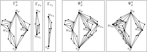
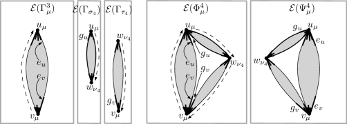
• First, we initialize both $\Phi^{i}_{\mu}$ and $\Psi^{i}_{\mu}$ to $\Gamma^{i-1}_{\mu}$.

• Second, we place the vertex $w_{\nu_{i}}$ in $\Phi^{i}_{\mu}$ and $\Psi^{i}_{\mu}$ with the two placements that realize the prescribed lengths of the edges $(u_{\mu},w_{\nu_{i}})$ and $(v_{\mu},w_{\nu_{i}})$; in particular, the placement of $w_{\nu_{i}}$ in $\Phi^{i}_{\mu}$ is such that the clockwise order of the vertices of the cycle $(u_{\mu},v_{\mu},w_{\nu_{i}})$ is $u_{\mu},w_{\nu_{i}},v_{\mu}$, while the placement of $w_{\nu_{i}}$ in $\Psi^{i}_{\mu}$ is such that the clockwise order of the vertices of the cycle $(u_{\mu},v_{\mu},w_{\nu_{i}})$ is $u_{\mu},v_{\mu},w_{\nu_{i}}$.

• Third, we insert $\Gamma_{\sigma_{i}}$ in $\Phi^{i}_{\mu}$ so that the representation of the edge $(u_{\mu},w_{\nu_{i}})$ in $\Gamma_{\sigma_{i}}$ coincides with the one in $\Phi^{i}_{\mu}$. We also insert $\Gamma_{\tau_{i}}$ in $\Phi^{i}_{\mu}$ so that the representation of the edge $(v_{\mu},w_{\nu_{i}})$ in $\Gamma_{\tau_{i}}$ coincides with the one in $\Phi^{i}_{\mu}$. This concludes the construction of $\Phi^{i}_{\mu}$. The insertion of $\Gamma_{\sigma_{i}}$ and $\Gamma_{\tau_{i}}$ in $\Psi^{i}_{\mu}$ in order to conclude the construction of $\Psi^{i}_{\mu}$ is done in the same way.

• Finally, we construct a plane embedding $\mathcal{E}(\Phi^{i}_{\mu})$ as follows:

  • We glue the lists of the edges incident to $u_{\mu}$ in $\mathcal{E}(\Gamma^{i-1}_{\mu})$ and $\mathcal{E}(\Gamma_{\sigma_{i}})$, so that, in the counter-clockwise order of the edges incident to $u_{\mu}$, the edge $e_{u}$ that enters $u_{\mu}$ when traversing in counter-clockwise order the boundary of the outer face of $\mathcal{E}(\Gamma^{i-1}_{\mu})$ comes immediately before the edge $g_{u}$ that enters $u_{\mu}$ when traversing in clockwise order the boundary of the outer face of $\mathcal{E}(\Gamma_{\sigma_{i}})$.

  • We glue the lists of the edges incident to $v_{\mu}$ in $\mathcal{E}(\Gamma^{i-1}_{\mu})$ and $\mathcal{E}(\Gamma_{\tau_{i}})$, so that, in the clockwise order of the edges incident to $v_{\mu}$, the edge $e_{v}$ that enters $v_{\mu}$ when traversing in clockwise order the boundary of the outer face of $\Gamma^{i-1}_{\mu}$ comes immediately before the edge $g_{v}$ that enters $v_{\mu}$ when traversing in counter-clockwise order the boundary of the outer face of $\Gamma_{\tau_{i}}$.

  • We let the cycle bounding the outer face of $\mathcal{E}(\Phi^{i}_{\mu})$ be composed of the path that goes from $v_{\mu}$ to $u_{\mu}$ in clockwise direction along the outer face of $\mathcal{E}(\Gamma^{i-1}_{\mu})$, of the path that goes from $u_{\mu}$ to $w_{\nu_{i}}$ in clockwise direction along the outer face of $\mathcal{E}(\Gamma_{\sigma_{i}})$, and of the path that goes from $w_{\nu_{i}}$ to $v_{\mu}$ in clockwise direction along the outer face of $\mathcal{E}(\Gamma_{\tau_{i}})$.

  We remark that $\mathcal{E}(\Phi^{i}_{\mu})$ is not necessarily the plane embedding of $\Phi^{i}_{\mu}$, in fact $\Phi^{i}_{\mu}$ might even be non-planar.

  A plane embedding $\mathcal{E}(\Psi^{i}_{\mu})$ is constructed analogously.

The straight-line realizations $\Phi^{i}_{\mu}$ and $\Psi^{i}_{\mu}$, together with the plane embeddings $\mathcal{E}(\Phi^{i}_{\mu})$ and $\mathcal{E}(\Psi^{i}_{\mu})$, are hence constructed in $O(n)$ time.

We remark that the plane embeddings $\mathcal{E}(\Phi^{i}_{\mu})$ and $\mathcal{E}(\Psi^{i}_{\mu})$ both place $G_{\nu_{i}}$ “externally” with respect to $G^{i-1}_{\mu}$. This is a main ingredient for bounding the running time of our algorithm. It is also not a loss of generality, because of the ordering that has been established for the children of $\mu$, as proved in the following lemma.

Lemma 24.

Consider a $u_{\mu}v_{\mu}$-external realization $\Gamma^{i}_{\mu}$ of $G^{i}_{\mu}$. Then the restriction of $\Gamma^{i}_{\mu}$ to $G_{\nu_{i}}$ lies in the outer face of the restriction of $\Gamma^{i}_{\mu}$ to $G^{i-1}_{\mu}$.

Proof.

Suppose, for a contradiction, that the restriction of $\Gamma^{i}_{\mu}$ to $G_{\nu_{i}}$ lies inside an internal face $f$ of the restriction of $\Gamma^{i}_{\mu}$ to $G^{i-1}_{\mu}$. In particular, the path $(u_{\mu},w_{\nu_{i}},v_{\mu})$ lies inside $f$ in $\Gamma^{i}_{\mu}$. Since $\Gamma^{i}_{\mu}$ is a $u_{\mu}v_{\mu}$-external realization of $G^{i}_{\mu}$, both $u_{\mu}$ and $v_{\mu}$ are incident to the outer face of $\Gamma^{i}_{\mu}$, hence it is possible to draw a Jordan arc $\mathcal{C}_{\mu}$ connecting $u_{\mu}$ and $v_{\mu}$ and lying in the outer face of $\Gamma^{i}_{\mu}$, except at its end-points. Now $\mathcal{C}_{\mu}$ and the path $(u_{\mu},w_{\nu_{i}},v_{\mu})$ form a closed curve which contains the edge $(u_{\mu},v_{\mu})$ on one side and a graph $G_{\nu_{j}}$ on the other side (as otherwise $f$ would be the outer face of $\Gamma^{i}_{\mu}$), for some $2\leq j<i$. However, this implies that the path $(u_{\mu},w_{\nu_{i}},v_{\mu})$ lies inside the triangle representing the $3$-cycle $(u_{\mu},w_{\nu_{j}},v_{\mu})$ in $\Gamma^{i}_{\mu}$. This contradicts the planarity of $\Gamma^{i}_{\mu}$; indeed, we have $\ell(\nu_{i})>\ell(\nu_{j})>\ell(\nu_{1})$, hence the length of the path $(u_{\mu},w_{\nu_{i}},v_{\mu})$ is larger than the lengths of the path $(u_{\mu},w_{\nu_{j}},v_{\mu})$ and of the edge $(u_{\mu},v_{\mu})$ in $\Gamma^{i}_{\mu}$. ∎

We now resume the description of how the algorithm constructs $\mathcal{R}^{i}_{\mu}$. By means of Theorem 3.1, we test in $O(n)$ time whether $\Phi^{i}_{\mu}$ is a planar straight-line realization respecting $\mathcal{E}(\Phi^{i}_{\mu})$. By the construction of $\mathcal{E}(\Phi^{i}_{\mu})$, the test is positive if and only if $\Phi^{i}_{\mu}$ is a $u_{\mu}v_{\mu}$-external realization of $G^{i}_{\mu}$. If the test is negative, then we discard $\Phi^{i}_{\mu}$. Otherwise, for every realization $\Lambda^{i}_{\mu}$ in $\mathcal{R}^{i}_{\mu}$, we test whether $\Phi^{i}_{\mu}$ is $u_{\mu}v_{\mu}$-equivalent to $\Lambda^{i}_{\mu}$ and, if it is, we discard $\Phi^{i}_{\mu}$. This can be done in $O(n)$ time by rotating and translating $\Phi^{i}_{\mu}$ so that the representation of the edge $(u_{\mu},v_{\mu})$ coincides with the one in $\Lambda^{i}_{\mu}$ and by then checking whether the vertices along on the boundary of the outer face of $\Phi^{i}_{\mu}$ have the same coordinates as the vertices along on the boundary of the outer face of $\Lambda^{i}_{\mu}$. If we did not discard $\Phi^{i}_{\mu}$, then we insert it into $\mathcal{R}^{i}_{\mu}$.

We process $\Psi^{i}_{\mu}$ analogously to $\Phi^{i}_{\mu}$.

After we have processed every triple of drawings $\Gamma^{i-1}_{\mu}\in\mathcal{R}^{i-1}_{\mu}$, $\Gamma_{\sigma_{i}}\in\mathcal{R}_{\sigma_{i}}$, and $\Gamma_{\tau_{i}}\in\mathcal{R}_{\tau_{i}}$, if the set $\mathcal{R}^{i}_{\mu}$ is empty, then we report that $G$ admits no planar straight-line realization, otherwise $\mathcal{R}^{i}_{\mu}$ is a minimal $u_{\mu}v_{\mu}$-complete set of $u_{\mu}v_{\mu}$-external realizations of $G^{i}_{\mu}$. The correctness of these conclusions is proved in the following lemma.

Lemma 25.

If $\mathcal{R}^{i}_{\mu}$ is empty, then $G$ admits no planar straight-line realization. Otherwise, $\mathcal{R}^{i}_{\mu}$ is a minimal $u_{\mu}v_{\mu}$-complete set of $u_{\mu}v_{\mu}$-external realizations of $G^{i}_{\mu}$.

Proof.

The main ingredient of the proof is the following claim: If $G^{i}_{\mu}$ admits a $u_{\mu}v_{\mu}$-external realization $\Lambda^{i}_{\mu}$, then $\mathcal{R}^{i}_{\mu}$ contains a $u_{\mu}v_{\mu}$-external realization that is $u_{\mu}v_{\mu}$-equivalent to $\Lambda^{i}_{\mu}$.

We prove the claim. For a contradiction, suppose that $G^{i}_{\mu}$ admits a $u_{\mu}v_{\mu}$-external realization $\Lambda^{i}_{\mu}$ and that $\mathcal{R}^{i}_{\mu}$ does not contain any $u_{\mu}v_{\mu}$-external realization that is $u_{\mu}v_{\mu}$-equivalent to $\Lambda^{i}_{\mu}$. We are going to replace parts of $\Lambda^{i}_{\mu}$ with realizations in $\mathcal{R}^{i-1}_{\mu}$, $\mathcal{R}_{\sigma_{i}}$, and $\mathcal{R}_{\tau_{i}}$, so to obtain a $u_{\mu}v_{\mu}$-external realization of $G^{i}_{\mu}$ that is constructed by the algorithm and that should hence have been inserted in $\mathcal{R}^{i}_{\mu}$ (unless a $u_{\mu}v_{\mu}$-equivalent $u_{\mu}v_{\mu}$-external realization of $G^{i}_{\mu}$ is already in $\mathcal{R}^{i}_{\mu}$), from which a contradiction follows.

Let $\Lambda^{i-1}_{\mu}$, $\Lambda_{\sigma_{i}}$, and $\Lambda_{\tau_{i}}$ be the restrictions of $\Lambda^{i}_{\mu}$ to $G^{i-1}_{\mu}$, $G_{\sigma_{i}}$, and $G_{\tau_{i}}$, respectively. By Lemma 24, we have that $\Lambda_{\sigma_{i}}$ and $\Lambda_{\tau_{i}}$ lie in the outer face of $\Lambda^{i-1}_{\mu}$; furthermore, the fact that $\Lambda^{i}_{\mu}$ is a $u_{\mu}v_{\mu}$-external realization directly implies that $\Lambda_{\sigma_{i}}$ and $\Lambda^{i-1}_{\mu}$ lie in the outer face of $\Lambda_{\tau_{i}}$ and that $\Lambda_{\tau_{i}}$ and $\Lambda^{i-1}_{\mu}$ lie in the outer face of $\Lambda_{\sigma_{i}}$.

Since $\mathcal{R}^{i-1}_{\mu}$ is a $u_{\mu}v_{\mu}$-complete set of $u_{\mu}v_{\mu}$-external realizations of $G^{i-1}_{\mu}$, it follows that there exists a $u_{\mu}v_{\mu}$-external realization $\Gamma^{i-1}_{\mu}\in\mathcal{R}^{i-1}_{\mu}$ of $G^{i-1}_{\mu}$ that is $u_{\mu}v_{\mu}$-equivalent to $\Lambda^{i-1}_{\mu}$. Analogously, there exists a $u_{\mu}w_{\nu_{i}}$-external realization $\Gamma_{\sigma_{i}}\in\mathcal{R}_{\sigma_{i}}$ of $G_{\sigma_{i}}$ that is $u_{\mu}w_{\nu_{i}}$-equivalent to $\Lambda_{\sigma_{i}}$ and there exists a $v_{\mu}w_{\nu_{i}}$-external realization $\Gamma_{\tau_{i}}\in\mathcal{R}_{\tau_{i}}$ of $G_{\tau_{i}}$ that is $v_{\mu}w_{\nu_{i}}$-equivalent to $\Lambda_{\tau_{i}}$.

We can now replace $\Lambda^{i-1}_{\mu}$ with $\Gamma^{i-1}_{\mu}$ in $\Lambda^{i}_{\mu}$, after rotating and translating $\Gamma^{i-1}_{\mu}$ so that the representation of the edge $(u_{\mu},v_{\mu})$ coincides with the one in $\Lambda^{i}_{\mu}$. Since the boundary of the outer face of $\Gamma^{i-1}_{\mu}$ coincides with the boundary of the outer face of $\Lambda^{i-1}_{\mu}$ and since $\Lambda_{\sigma_{i}}$ and $\Lambda_{\tau_{i}}$ lie in the outer face of $\Lambda^{i-1}_{\mu}$, it follows that after the replacement $\Lambda^{i}_{\mu}$ remains a $u_{\mu}v_{\mu}$-external realization of $G^{i}_{\mu}$ (in particular, it remains planar) that is $u_{\mu}v_{\mu}$-equivalent to $\Lambda^{i}_{\mu}$. We can analogously replace $\Lambda_{\sigma_{i}}$ with $\Gamma_{\sigma_{i}}$ and $\Lambda_{\tau_{i}}$ with $\Gamma_{\tau_{i}}$, obtaining a $u_{\mu}v_{\mu}$-external realization of $G_{\mu}$ that is constructed by the algorithm and that is $u_{\mu}v_{\mu}$-equivalent to $\Lambda^{i}_{\mu}$. This implies that $\mathcal{R}^{i}_{\mu}$ contains a $u_{\mu}v_{\mu}$-external realization that is $u_{\mu}v_{\mu}$-equivalent to $\Lambda^{i}_{\mu}$, a contradiction which proves the claim.

The claim directly implies that, if $\mathcal{R}^{i}_{\mu}$ is empty, then $G^{i}_{\mu}$ admits no $u_{\mu}v_{\mu}$-external realization, hence $G_{\mu}$ admits no $u_{\mu}v_{\mu}$-external realization (given that $G^{i}_{\mu}$ is a subgraph of $G_{\mu}$), and finally that $G$ admits no planar straight-line realization, by Lemma 23.

Suppose now that $\mathcal{R}^{i}_{\mu}$ is non-empty. We prove that $\mathcal{R}^{i}_{\mu}$ is a minimal $u_{\mu}v_{\mu}$-complete set of $u_{\mu}v_{\mu}$-external realizations of $G^{i}_{\mu}$. First, that every realization $\Gamma^{i}_{\mu}$ in $\mathcal{R}^{i}_{\mu}$ is $u_{\mu}v_{\mu}$-external directly descends from the $O(n)$-time test that is performed by means of Theorem 3.1 on $\Gamma^{i}_{\mu}$; indeed, $\Gamma^{i}_{\mu}$ is inserted into $\mathcal{R}^{i}_{\mu}$ only if the test reports that $\Gamma^{i}_{\mu}$ is a planar straight-line realization whose plane embedding is the one constructed by the algorithm, in which $u_{\mu}$ and $v_{\mu}$ are incident to the outer face. Second, that $\mathcal{R}^{i}_{\mu}$ is $u_{\mu}v_{\mu}$-complete is a direct consequence of the claim above. Finally, the minimality of $\mathcal{R}^{i}_{\mu}$ comes from the fact that a realization is inserted into $\mathcal{R}^{i}_{\mu}$ only if it is not $u_{\mu}v_{\mu}$-equivalent to any realization already in $\mathcal{R}^{i}_{\mu}$. ∎

It remains to determine the running time of our algorithm. The main ingredient we are going to use is the following combinatorial lemma.

Lemma 26.

Let $\mu$ be a Q-node or a P-node of $\mathcal{T}$, and let $h$ be the height of ${\mathcal{T}}_{\mu}$. We have that $|\mathcal{R}_{\mu}|\leq n^{\frac{2^{h}-1}{3}}\cdot 2^{\frac{2^{h}-1}{3}}$. Furthermore, if $\mu$ is a P-node, let $\nu_{1},\dots,\nu_{k}$ be the children of $\mu$. For $i=1,\dots,k$, we have that $|\mathcal{R}^{i}_{\mu}|\leq n^{\frac{2^{h}-1}{3}}\cdot 2^{\frac{2^{h}-1}{3}}$.

Proof.

We prove the following claim. Let $f(k)$ be the function whose domain consists of the even natural numbers, that is recursively defined as follows: $f(k)=1$ if $k=0$, and $f(k)=2n\cdot(f(k-2))^{4}$ if $k>0$. Then we claim that $|\mathcal{R}_{\mu}|\leq f(h)$ and $|\mathcal{R}^{i}_{\mu}|\leq f(h)$. The claim implies the lemma, as an easy inductive proof shows that the closed form of $f(k)$ is $f(k)=n^{\frac{2^{k}-1}{3}}\cdot 2^{\frac{2^{k}-1}{3}}$.

The claim is proved by induction on $h$. If $h=0$, then $\mu$ is a Q-node, hence by construction we have that $|\mathcal{R}_{\mu}|=1=f(0)$.

Suppose now that $h>0$, hence $\mu$ is a P-node with children $\nu_{1},\dots,\nu_{k}$. First, we have $\mathcal{R}^{1}_{\mu}=1<f(h)$. We now prove that $|\mathcal{R}^{i}_{\mu}|\leq n^{\frac{2^{h}-1}{3}}\cdot 2^{\frac{2^{h}-1}{3}}$, for any $i\in\{2,\dots,k\}$; this suffices to complete the induction, since by construction $\mathcal{R}_{\mu}=\mathcal{R}^{k}_{\mu}$. Consider any realization $\Gamma^{i}_{\mu}$ in $\mathcal{R}^{i}_{\mu}$. Since $\Gamma^{i}_{\mu}$ is a $u_{\mu}v_{\mu}$-external realization of $G^{i}_{\mu}$ and since $i\geq 2$, it follows that there are exactly two graphs among $G_{\nu_{1}},\dots,G_{\nu_{i}}$ that contain edges incident to the outer face of $\Gamma^{i}_{\mu}$. By Lemma 24, one of these graphs is $G_{\nu_{i}}$, while the other graph, say $G_{\nu_{j}}$, might be any graph among $G_{\nu_{1}},\dots,G_{\nu_{i-1}}$. When traversing the boundary of the outer face of $\Gamma^{i}_{\mu}$ in clockwise direction, the edge $e_{\nu_{i}}$ of $G_{\nu_{i}}$ incident to $u_{\mu}$ might appear right before or right after $u_{\mu}$. Altogether, there are less than $2n$ possibilities for the choice of the graph $G_{\nu_{j}}$ and for whether $e_{\nu_{i}}$ appears right before or right after $u_{\mu}$ in clockwise order along the boundary of the outer face of $\Gamma^{i}_{\mu}$. For each of these $2n$ possibilities, the interior of $\Gamma^{i}_{\mu}$ is determined by the choice of four realizations $\Gamma_{\sigma_{i}}\in\mathcal{R}_{\sigma_{i}}$, $\Gamma_{\tau_{i}}\in\mathcal{R}_{\tau_{i}}$, $\Gamma_{\sigma_{j}}\in\mathcal{R}_{\sigma_{j}}$, and $\Gamma_{\tau_{j}}\in\mathcal{R}_{\tau_{j}}$. Indeed, the restriction of $\Gamma^{i}_{\mu}$ to $G_{\sigma_{i}}$, $G_{\tau_{i}}$, $G_{\sigma_{j}}$, and $G_{\tau_{j}}$ is a realization in $\mathcal{R}_{\sigma_{i}}$, $\mathcal{R}_{\tau_{i}}$, $\mathcal{R}_{\sigma_{j}}$, and $\mathcal{R}_{\tau_{j}}$, respectively. Since the heights of $\mathcal{T}_{\sigma_{i}}$, $\mathcal{T}_{\tau_{i}}$, $\mathcal{T}_{\sigma_{j}}$, and $\mathcal{T}_{\tau_{j}}$ are each at most $h-2$, by induction each of $\mathcal{R}_{\sigma_{i}}$, $\mathcal{R}_{\tau_{i}}$, $\mathcal{R}_{\sigma_{j}}$, and $\mathcal{R}_{\tau_{j}}$ has size smaller than or equal to $f(h-2)$. Hence, the number of possible choices for the realizations $\Gamma_{\sigma_{i}}\in\mathcal{R}_{\sigma_{i}}$, $\Gamma_{\tau_{i}}\in\mathcal{R}_{\tau_{i}}$, $\Gamma_{\sigma_{j}}\in\mathcal{R}_{\sigma_{j}}$, and $\Gamma_{\tau_{j}}\in\mathcal{R}_{\tau_{j}}$ is smaller than or equal to $(f(h-2))^{4}$. Finally, the minimality of $\mathcal{R}^{i}_{\mu}$ implies that no two realizations in $\mathcal{R}^{i}_{\mu}$ coincide when restricted to $G_{\sigma_{i}}$, $G_{\tau_{i}}$, $G_{\sigma_{j}}$, and $G_{\tau_{j}}$. This proves that the number of realizations in $\mathcal{R}^{i}_{\mu}$ is smaller than or equal to $2n\cdot(f(h-2))^{4}$; this concludes the induction and hence the proof of the lemma. ∎

We are now ready to determine the running time of our algorithm. Whenever a P-node $\mu$ with $k$ children $\nu_{1},\dots,\nu_{k}$ is visited in the bottom-up traversal of $\mathcal{T}$, for $i=1,\dots,k$, the set $\mathcal{R}^{i}_{\mu}$ is constructed by considering every triple of drawings $\Gamma^{i-1}_{\mu}\in\mathcal{R}^{i-1}_{\mu}$, $\Gamma_{\sigma_{i}}\in\mathcal{R}_{\sigma_{i}}$, and $\Gamma_{\tau_{i}}\in\mathcal{R}_{\tau_{i}}$, where $\sigma_{i}$ and $\tau_{i}$ are the children of $\nu_{i}$. By Lemma 26, the number of such triples is at most $\big{(}n^{\frac{2^{h^{*}}-1}{3}}\cdot 2^{\frac{2^{h^{*}}-1}{3}}\big{)}\big{(}n^{\frac{2^{(h^{*}-2)}-1}{3}}\cdot 2^{\frac{2^{(h^{*}-2)}-1}{3}}\big{)}^{2}=n^{(2^{(h^{*}-1)}-1)}\cdot 2^{(2^{(h^{*}-1)}-1)}$; indeed, the height of $\mathcal{T}$ is $h^{*}$, hence the height of $\mathcal{T}_{\mu}$ is smaller than or equal to $h^{*}$, and the heights of $\mathcal{T}_{\sigma_{i}}$ and $\mathcal{T}_{\tau_{i}}$ are smaller than or equal to $h^{*}-2$. For each of such triples, two straight-line realizations $\Phi^{i}_{\mu}$ and $\Psi^{i}_{\mu}$ are constructed in $O(n)$ time, together with the plane embeddings $\mathcal{E}(\Phi^{i}_{\mu})$ and $\mathcal{E}(\Psi^{i}_{\mu})$. By means of Theorem 3.1, it is tested in $O(n)$ time whether $\Phi^{i}_{\mu}$ and $\Psi^{i}_{\mu}$ are planar straight-line realizations with plane embeddings $\mathcal{E}(\Phi^{i}_{\mu})$ and $\mathcal{E}(\Psi^{i}_{\mu})$, respectively. For each realization $\Lambda^{i}_{\mu}$ of $G^{i}_{\mu}$ in $\mathcal{R}^{i}_{\mu}$, it is tested in $O(n)$ time whether $\Phi^{i}_{\mu}$ is $u_{\mu}v_{\mu}$-equivalent to $\Lambda^{i}_{\mu}$. By Lemma 26, the set $\mathcal{R}^{i}_{\mu}$ contains at most $\big{(}n^{\frac{2^{h^{*}}-1}{3}}\cdot 2^{\frac{2^{h^{*}}-1}{3}}\big{)}$ realizations of $G^{i}_{\mu}$, hence these $O(n)$-time tests are performed $\big{(}n^{(2^{(h^{*}-1)}-1)}\cdot 2^{(2^{(h^{*}-1)}-1)}\big{)}\big{(}n^{\frac{2^{h^{*}}-1}{3}}\cdot 2^{\frac{2^{h^{*}}-1}{3}}\big{)}=\big{(}n^{\frac{5\cdot 2^{h^{*}-1}-4}{3}}\cdot 2^{\frac{5\cdot 2^{h^{*}-1}-4}{3}}\big{)}$ times, with a $\big{(}n^{\frac{5\cdot 2^{h^{*}-1}-1}{3}}\cdot 2^{\frac{5\cdot 2^{h^{*}-1}-4}{3}}\big{)}$ running time. Since the number of P-nodes in $\mathcal{T}$ is in $O(n)$, the running time of our algorithm is in $\big{(}n^{\frac{5\cdot 2^{h^{*}-1}+2}{3}}\cdot 2^{\frac{5\cdot 2^{h^{*}-1}-4}{3}}\big{)}\in n^{O(2^{h^{*}})}$. This concludes the proof of Theorem 7.1.

8 Conclusions and Open Problems

We studied the problem of testing if a $2$-tree has a planar straight-line drawing with prescribed edge lengths, both when the number of distinct edge lengths is bounded and when it is unbounded.

In the bounded setting, we proved that the problem is linear-time solvable if the number of prescribed distinct lengths is at most two, while it is -hard if this number is four or more. Hence, an intriguing question is to determine the complexity of the problem for weighted graphs with three prescribed distinct lengths.

In the unbounded setting, we showed that the problem is linear-time solvable if the embedding of the input graph is prescribed. Moreover, we studied weighted maximal outerplanar graphs, and we proved that the problem is linear-time solvable if their dual tree is a path, and cubic-time solvable if their dual tree is a caterpillar. We leave open the problem about general maximal outerplanar graphs.

Finally, for the general problem on weighted $2$-trees, we described a slice-wise polynomial-time algorithm, parameterized by the length of the longest path. A natural open problem is to determine whether the problem admits an FPT algorithm with respect to the same parameter.

References

- [1] Abel, Z., Demaine, E.D., Demaine, M.L., Eisenstat, S., Lynch, J., Schardl, T.B.: Who needs crossings? Hardness of plane graph rigidity. In: Fekete, S.P., Lubiw, A. (eds.) 32nd International Symposium on Computational Geometry (SoCG ’16). LIPIcs, vol. 51, pp. 3:1–3:15. Schloss Dagstuhl - Leibniz-Zentrum für Informatik (2016). https://doi.org/10.4230/LIPIcs.SoCG.2016.3
- [2] Aichholzer, O., Kusters, V., Mulzer, W., Pilz, A., Wettstein, M.: An optimal algorithm for reconstructing point set order types from radial orderings. Int. J. Comput. Geom. Appl. 27(1-2), 57–84 (2017)
- [3] Alon, N., Feldheim, O.N.: Drawing outerplanar graphs using three edge lengths. Comput. Geom. 48(3), 260–267 (2015). https://doi.org/10.1016/j.comgeo.2014.10.006
- [4] Angelini, P., Da Lozzo, G., Di Bartolomeo, M., Di Battista, G., Hong, S., Patrignani, M., Roselli, V.: Anchored drawings of planar graphs. In: Duncan, C.A., Symvonis, A. (eds.) 22nd International Symposium on Graph Drawing (GD ’14). Lecture Notes in Computer Science, vol. 8871, pp. 404–415. Springer (2014). https://doi.org/10.1007/978-3-662-45803-7_34
- [5] Angelini, P., Da Lozzo, G., Di Battista, G., Di Donato, V., Kindermann, P., Rote, G., Rutter, I.: Windroe planarity: Embedding graphs with direction-constrained edges. ACM Trans. Algorithms 14(4), 54:1–54:24 (2018). https://doi.org/10.1145/3239561
- [6] Aspvall, B., Plass, M.F., Tarjan, R.E.: A linear-time algorithm for testing the truth of certain quantified boolean formulas. Information Processing Letters 8(3), 121–123 (1979). https://doi.org/10.1016/0020-0190(79)90002-4
- [7] Ben-Or, M.: Lower bounds for algebraic computation trees (preliminary report). In: Johnson, D.S., Fagin, R., Fredman, M.L., Harel, D., Karp, R.M., Lynch, N.A., Papadimitriou, C.H., Rivest, R.L., Ruzzo, W.L., Seiferas, J.I. (eds.) 15th Annual ACM Symposium on Theory of Computing (STOC ’83). pp. 80–86. ACM (1983). https://doi.org/10.1145/800061.808735
- [8] de Berg, M., Khosravi, A.: Optimal binary space partitions for segments in the plane. Int. J. Comput. Geom. Appl. 22(3), 187–206 (2012). https://doi.org/10.1142/S0218195912500045
- [9] Berger, B., Kleinberg, J.M., Leighton, F.T.: Reconstructing a three-dimensional model with arbitrary errors. J. ACM 46(2), 212–235 (1999). https://doi.org/10.1145/301970.301972
- [10] Blazej, V., Fiala, J., Liotta, G.: On the edge-length ratio of 2-trees. In: Auber, D., Valtr, P. (eds.) 28th International Symposium on Graph Drawing and Network Visualization (GD ’20). Lecture Notes in Computer Science, vol. 12590, pp. 85–98. Springer (2020). https://doi.org/10.1007/978-3-030-68766-3_7
- [11] Borrazzo, M., Frati, F.: On the planar edge-length ratio of planar graphs. J. Comput. Geom. 11(1), 137–155 (2020). https://doi.org/10.20382/jocg.v11i1a6
- [12] Brandes, U., Schlieper, B.: Angle and distance constraints on tree drawings. In: Kaufmann, M., Wagner, D. (eds.) 14th International Symposium on Graph Drawing (GD ’06). Lecture Notes in Computer Science, vol. 4372, pp. 54–65. Springer (2006). https://doi.org/10.1007/978-3-540-70904-6_7
- [13] Brandstädt, A., Le, V.B., Spinrad, J.P.: Graph Classes: A Survey. SIAM Monographs on Discrete Mathematics and Applications, SIAM (1999)
- [14] Cabello, S., Demaine, E.D., Rote, G.: Planar embeddings of graphs with specified edge lengths. Journal of Graph Algorithms and Applications 11(1), 259–276 (2007). https://doi.org/10.7155/jgaa.00145
- [15] Capkun, S., Hamdi, M., Hubaux, J.: GPS-free positioning in mobile ad hoc networks. Clust. Comput. 5(2), 157–167 (2002). https://doi.org/10.1023/A:1013933626682
- [16] Chaplick, S., Kindermann, P., Löffler, A., Thiele, F., Wolff, A., Zaft, A., Zink, J.: Recognizing stick graphs with and without length constraints. J. Graph Algorithms Appl. 24(4), 657–681 (2020). https://doi.org/10.7155/jgaa.00524
- [17] Chazelle, B.: Triangulating a simple polygon in linear time. Discret. Comput. Geom. 6, 485–524 (1991). https://doi.org/10.1007/BF02574703
- [18] Connelly, R.: On generic global rigidity. In: Gritzmann, P., Sturmfels, B. (eds.) Proceedings of a DIMACS Workshop on Applied Geometry And Discrete Mathematics. DIMACS Series in Discrete Mathematics and Theoretical Computer Science, vol. 4, pp. 147–156. DIMACS/AMS (1990). https://doi.org/10.1090/dimacs/004/11
- [19] Coullard, C.R., Lubiw, A.: Distance visibility graphs. Int. J. Comput. Geom. Appl. 2(4), 349–362 (1992). https://doi.org/10.1142/S0218195992000202
- [20] Da Lozzo, G., Devanny, W.E., Eppstein, D., Johnson, T.: Square-contact representations of partial 2-trees and triconnected simply-nested graphs. In: Okamoto, Y., Tokuyama, T. (eds.) 28th International Symposium on Algorithms and Computation (ISAAC ’17). LIPIcs, vol. 92, pp. 24:1–24:14. Schloss Dagstuhl - Leibniz-Zentrum für Informatik (2017). https://doi.org/10.4230/LIPIcs.ISAAC.2017.24
- [21] Deng, T.: On the implementation and refinement of outerplanar graph algorithms. Master’s thesis, University of Windsor, Ontario, Canada (2007)
- [22] Devillers, O., Liotta, G., Preparata, F.P., Tamassia, R.: Checking the convexity of polytopes and the planarity of subdivisions. Comput. Geom. 11(3-4), 187–208 (1998). https://doi.org/10.1016/S0925-7721(98)00039-X
- [23] Di Battista, G., Eades, P., Tamassia, R., Tollis, I.G.: Graph Drawing: Algorithms for the Visualization of Graphs. Prentice-Hall (1999)
- [24] Di Battista, G., Tamassia, R.: On-line planarity testing. SIAM J. Comput. 25(5), 956–997 (1996). https://doi.org/10.1137/S0097539794280736
- [25] Di Battista, G., Tamassia, R., Tollis, I.G.: Constrained visibility representations of graphs. Inf. Process. Lett. 41(1), 1–7 (1992). https://doi.org/10.1016/0020-0190(92)90072-4
- [26] Di Giacomo, E., Didimo, W., Liotta, G.: Radial drawings of graphs: Geometric constraints and trade-offs. J. Discrete Algorithms 6(1), 109–124 (2008). https://doi.org/10.1016/j.jda.2006.12.007
- [27] Di Giacomo, E., Hancl, J., Liotta, G.: 2-colored point-set embeddings of partial 2-trees. In: Uehara, R., Hong, S., Nandy, S.C. (eds.) 15th International Conference and Workshops on Algorithms and Computation (WALCOM ’21). Lecture Notes in Computer Science, vol. 12635, pp. 247–259. Springer (2021). https://doi.org/10.1007/978-3-030-68211-8_20
- [28] Eades, P., Wormald, N.C.: Fixed edge-length graph drawing is NP-hard. Disc. Appl. Math. 28(2), 111–134 (1990). https://doi.org/10.1016/0166-218X(90)90110-X
- [29] Geelen, J., Guo, A., McKinnon, D.: Straight line embeddings of cubic planar graphs with integer edge lengths. J. Graph Theory 58(3), 270–274 (2008). https://doi.org/10.1002/jgt.20304
- [30] Goodrich, M.T., Johnson, T.: Low ply drawings of trees and 2-trees. In: Durocher, S., Kamali, S. (eds.) Proceedings of the 30th Canadian Conference on Computational Geometry (CCCG ’18). pp. 2–10 (2018), http://www.cs.umanitoba.ca/%7Ecccg2018/papers/session1A-p1.pdf
- [31] Gutwenger, C., Mutzel, P.: A linear time implementation of SPQR-trees. In: Marks, J. (ed.) 8th International Symposium on Graph Drawing (GD ’00). LNCS, vol. 1984, pp. 77–90 (2000). https://doi.org/10.1007/3-540-44541-2_8
- [32] Hendrickson, B.: Conditions for unique graph realizations. SIAM J. Comput. 21(1), 65–84 (1992). https://doi.org/10.1137/0221008
- [33] Hendrickson, B.: The molecule problem: Exploiting structure in global optimization. SIAM J. Optim. 5(4), 835–857 (1995). https://doi.org/10.1137/0805040
- [34] Jackson, B., Jordán, T.: Connected rigidity matroids and unique realizations of graphs. J. Comb. Theory, Ser. B 94(1), 1–29 (2005). https://doi.org/10.1016/j.jctb.2004.11.002
- [35] Lenhart, W., Liotta, G., Mondal, D., Nishat, R.I.: Planar and plane slope number of partial 2-trees. In: Wismath, S.K., Wolff, A. (eds.) 21st International Symposium on Graph Drawing (GD ’13). Lecture Notes in Computer Science, vol. 8242, pp. 412–423. Springer (2013). https://doi.org/10.1007/978-3-319-03841-4_36
- [36] Lubiw, A., Miltzow, T., Mondal, D.: The complexity of drawing a graph in a polygonal region. In: Biedl, T.C., Kerren, A. (eds.) 26th International Symposium on Graph Drawing and Network Visualization (GD ’18). Lecture Notes in Computer Science, vol. 11282, pp. 387–401. Springer (2018). https://doi.org/10.1007/978-3-030-04414-5_28
- [37] Melkman, A.A.: On-line construction of the convex hull of a simple polyline. Inf. Process. Lett. 25(1), 11–12 (1987). https://doi.org/10.1016/0020-0190(87)90086-X
- [38] Mitchell, S.L.: Linear algorithms to recognize outerplanar and maximal outerplanar graphs. Inf. Process. Lett. 9(5), 229–232 (1979). https://doi.org/10.1016/0020-0190(79)90075-9
- [39] Moran, S., Wolfstahl, Y.: One-page book embedding under vertex-neighborhood constraints. SIAM J. Discrete Math. 3(3), 376–390 (1990). https://doi.org/10.1137/0403034
- [40] Priyantha, N.B., Chakraborty, A., Balakrishnan, H.: The cricket location-support system. In: Pickholtz, R.L., Das, S.K., Cáceres, R., Garcia-Luna-Aceves, J.J. (eds.) 6th Annual International Conference on Mobile Computing and Networking (MOBICOM ’00). pp. 32–43. ACM (2000). https://doi.org/10.1145/345910.345917
- [41] Rengarajan, S., Madhavan, C.E.V.: Stack and queue number of 2-trees. In: Du, D., Li, M. (eds.) First Annual International Conference on Computing and Combinatorics (COCOON ’95). Lecture Notes in Computer Science, vol. 959, pp. 203–212. Springer (1995). https://doi.org/10.1007/BFb0030834
- [42] Rosenstiehl, P., Tarjan, R.E.: Rectilinear planar layouts and bipolar orientations of planar graphs. Discret. Comput. Geom. 1, 343–353 (1986). https://doi.org/10.1007/BF02187706
- [43] Savarese, C., Rabaey, J., Beutel, J.: Location in distributed ad-hoc wireless sensor networks. In: 2001 IEEE International Conference on Acoustics, Speech, and Signal Processing. Proceedings. vol. 4, pp. 2037–2040 (2001). https://doi.org/10.1109/ICASSP.2001.940391
- [44] Saxe, J.: Embeddability of Weighted Graphs in K-space is Strongly NP-hard. CMU-CS-80-102, Carnegie-Mellon University, Department of Computer Science (1980), https://books.google.it/books?id=vClAGwAACAAJ
- [45] Schaefer, M.: Realizability of graphs and linkages. In: Pach, J. (ed.) Thirty Essays on Geometric Graph Theory, pp. 461–482. Springer New York, New York, NY (2013). https://doi.org/10.1007/978-1-4614-0110-0_24
- [46] Silveira, R.I., Speckmann, B., Verbeek, K.: Non-crossing paths with geographic constraints. Discret. Math. Theor. Comput. Sci. 21(3) (2019). https://doi.org/10.23638/DMTCS-21-3-15
- [47] Syslo, M.M.: Characterizations of outerplanar graphs. Discret. Math. 26(1), 47–53 (1979). https://doi.org/10.1016/0012-365X(79)90060-8
- [48] Tamassia, R.: Constraints in graph drawing algorithms. Constraints An Int. J. 3(1), 87–120 (1998). https://doi.org/10.1023/A:1009760732249
- [49] Valdes, J., Tarjan, R.E., Lawler, E.L.: The recognition of series parallel digraphs. SIAM J. Comput. 11(2), 298–313 (1982)
- [50] Wiegers, M.: Recognizing outerplanar graphs in linear time. In: Tinhofer, G., Schmidt, G. (eds.) Graph-Theoretic Concepts in Computer Science (WG ’86). LNCS, vol. 246, pp. 165–176. Springer Berlin Heidelberg (1987). https://doi.org/10.1007/3-540-17218-1_57
- [51] Yemini, Y.: Some theoretical aspects of position-location problems. In: 20th Annual Symposium on Foundations of Computer Science (FOCS ’79). pp. 1–8. IEEE Computer Society (1979). https://doi.org/10.1109/SFCS.1979.39