Revisiting Event Study Designs:
Robust and Efficient Estimation

Abstract

We develop a framework for difference-in-differences designs with staggered treatment adoption and heterogeneous causal effects. We show that conventional regression-based estimators fail to provide unbiased estimates of relevant estimands absent strong restrictions on treatment-effect homogeneity. We then derive the efficient estimator addressing this challenge, which takes an intuitive “imputation” form when treatment-effect heterogeneity is unrestricted. We characterize the asymptotic behavior of the estimator, propose tools for inference, and develop tests for identifying assumptions. Our method applies with time-varying controls, in triple-difference designs, and with certain non-binary treatments. We show the practical relevance of our results in a simulation study and an application. Studying the consumption response to tax rebates in the United States, we find that the notional marginal propensity to consume is between 8 and 11 percent in the first quarter — about half as large as benchmark estimates used to calibrate macroeconomic models — and predominantly occurs in the first month after the rebate.

1 Introduction

Event studies are one of the most popular tools in applied economics and policy evaluation. An event study is a difference-in-differences (DiD) design in which a set of units in the panel receive treatment at different points in time. In this paper, we investigate the robustness and efficiency of estimators of causal effects in event studies, with a focus on the role of treatment effect heterogeneity. We first develop a simple econometric framework that delineates the identification assumptions from each other and from the estimation target, defined as some average of heterogeneous causal effects. We then apply this framework in three ways. First, we analyze the conventional practice of implementing event studies via two-way fixed effect Ordinary Least Squares (TWFE OLS) regressions and show how the implicit conflation of different assumptions leads to biases. Second, leveraging event study assumptions in an explicit and principled way allows us to derive the robust and efficient estimator, along with appropriate inference methods and tests. The estimator takes an intuitive “imputation” form when treatment-effect heterogeneity is unrestricted. Finally, we illustrate the practical relevance of our approach in an application estimating the marginal propensity to spend (MPX) out of tax rebates; our MPX estimates are lower than in prior work, implying that fiscal stimulus is less powerful than commonly thought.

Event studies are frequently used to estimate treatment effects when treatment is not randomized, but the researcher has panel data allowing them to compare outcome trajectories before and after the onset of treatment, as well as across units treated at different times. By analogy to conventional DiD designs without staggered rollout, event studies are commonly implemented by two-way fixed effect regressions, such as

$$Y_{it} =\alpha_{i}+\beta_{t}+\tau D_{it}+\varepsilon_{it},$$ (1)

where outcome $Y_{it}$ and binary treatment $D_{it}$ are measured in periods $t$ and for units $i$, $\alpha_{i}$ are unit fixed effects (FEs) that allow for different baseline outcomes across units, and $\beta_{t}$ are period fixed effects that accommodate overall trends in the outcome. Specifications like Equation 1 are meant to isolate a treatment effect $\tau$ from unit- and period-specific confounders. A commonly-used dynamic version of this regression includes “lags” and “leads” of the indicator for the onset of treatment, to capture treatment effects for different “horizons” since the onset of treatment and test for the parallel trajectories of the pre-treatment outcomes.

To understand the problems with conventional two-way fixed effect estimators in event-study designs and provide a principled econometric approach to overcoming these issues, in Section 2 we develop a simple framework that makes the estimation targets and underlying assumptions explicit and clearly isolated. We suppose that the researcher chooses a particular weighted average (or weighted sum) of heterogeneous treatment effects they are interested in estimating. We make (and later test) two standard DiD identification assumptions: that potential outcomes without treatment are characterized by parallel trends and that there are no anticipatory effects. We also allow for — but do not require — an auxiliary assumption that the treatment effects themselves follow some model that restricts their heterogeneity for a priori specified economic reasons. This explicit approach is in contrast to regression specifications like Equation 1, both static and dynamic, which implicitly conflate choices of estimation target and identification assumptions. Our framework covers a broad class of empirically relevant estimands beyond the standard average treatment-on-the-treated (ATT), including heterogeneous treatment effects by observed covariates and ATTs at different horizons that hold the composition of units fixed.

Through the lens of this framework, in Section 3 we uncover a set of challenges with conventional event-study estimation methods and trace them back to a mismatch between estimation target, identification assumptions, and the flexibility of the regression specification. First, we note that failing to rule out anticipation effects in “fully-dynamic” specifications (with all leads and lags of the event included) leads to an underidentification problem when there are no never-treated units, such that the dynamic path of anticipation and treatment effects over time is not point-identified. We conclude that it is important to separate out testing the assumptions about pre-trends from the estimation of dynamic treatment effects under those assumptions. Second, implicit assumptions of homogeneous treatment effects embedded in static DiD regressions like Equation 1 may lead to estimands that put negative weights on some long-run treatment effects. With staggered rollout, regression-based estimation leverages comparisons between groups that got treated over a period of time and reference groups which had been treated earlier. We label such cases “forbidden comparisons.” Indeed, these comparisons are only valid when the homogeneity assumption is true; when it is violated, they can substantially distort the weights the estimator places on treatment effects, or even make them negative. Third, in dynamic specifications, implicit assumptions about treatment effect homogeneity across groups first treated at different times lead to the spurious identification of long-run treatment effects for which no DiD comparisons valid under heterogeneous treatment effects are available. The last two challenges highlight the danger of imposing implicit treatment effect homogeneity assumptions instead of allowing for heterogeneity and explicitly specifying the target estimand. We show that these challenges are not resolved by trimming the sample to a fixed window around the event date.

From the above discussion, the reader should not conclude that event study designs are plagued by fundamental problems. On the contrary, these challenges only arise due to a mismatch between treatment effect heterogeneity and specifications which restrict it. We therefore use our framework to circumvent these issues and derive robust and efficient estimators.

In Section 4, we first establish a simple characterization for the most efficient linear unbiased estimator of any pre-specified weighted sum of treatment effects, in the baseline case of spherical errors, i.e. homoskedasticity with no serial correlation. This estimator explicitly incorporates the researcher’s estimation goal and assumptions about parallel trends, anticipation effects, and restrictions on treatment effect heterogeneity. It is constructed by estimating a flexible high-dimensional regression that differs from conventional event study specifications, and aggregating its coefficients appropriately. While spherical errors are a natural starting point, the principled construction of this estimator more generally ensures unbiasedness and yields attractive efficiency properties, as we later confirm in simulations.

In our leading case where the heterogeneity of treatment effects is not restricted, the efficient robust estimator can be implemented using a transparent “imputation” procedure. First, the unit and period fixed effects $\hat{\alpha}_{i}$ and $\hat{\beta}_{t}$ are fitted by regressions using untreated observations only. Second, these fixed effects are used to impute the untreated potential outcomes and therefore obtain an estimated treatment effect $\hat{\tau}_{it}=Y_{it}-\hat{\alpha}_{i}-\hat{\beta}_{t}$ for each treated observation. Finally, a weighted sum of these treatment effect estimates is taken, with weights corresponding to the estimation target.

To relate our efficient imputation estimator to other unbiased estimators that have been proposed in the literature, we derive two additional results showing the generality of the imputation structure. First, any other linear estimator that is unbiased in our framework with unrestricted causal effects can be represented as an imputation estimator, albeit with an inefficient way of imputing untreated potential outcomes. Second, even when assumptions that restrict treatment effect heterogeneity are imposed, any unbiased estimator can still be understood as an imputation estimator for an adjusted estimand. Together, these two results allow us to characterize estimators of treatment effects in event studies as a combination of how they impute unobserved potential outcomes and which weights they put on treatment effects.

For the efficient estimator in our framework, we provide tools for valid inference. Specifically, we derive conditions under which the estimator is consistent and asymptotically normal and propose standard error estimates. Inference is challenging under arbitrary treatment effect heterogeneity, because causal effects cannot be separated from the error terms. We instead show how asymptotically conservative standard errors can be derived, by attributing some variation in estimated treatment effects to the error terms. Our inference results apply under mild conditions in short panels. Advancing the existing literature on DiD estimation with staggered adoption, we also provide conditions for consistency and inference that extend to panels where the number of time periods grows, as long as growth is not too fast. We also propose a leave-one-out modification to our conservative variance estimates with improved finite-sample performance.

Another important practical advantage of our approach is that it provides a principled way of testing the identifying assumptions of parallel trends and no anticipation effects, based on OLS regressions with untreated observations only. Compared to conventional specifications with leads and lags of treatment that implicitly restrict treatment effects, this approach avoids the contamination of the tests by treatment effect heterogeneity shown by [60]. Moreover, our strategy circumvents the inference problems after pre-testing that were pointed out by [37], under spherical errors. These attractive properties result from the clear separation of estimation and testing.

It is also useful to point out two limitations of our analysis. First, all event study designs assume a restrictive parametric model for untreated outcomes. We do not evaluate when these assumptions may be applicable, and therefore when the event study design are ex ante appropriate, as [39] do. We similarly do not consider estimation that is robust to violations of parallel-trend type assumptions, as [36] propose, although our framework allows relaxing those assumptions by including unit-specific trends and time-varying covariates. We instead take the standard assumptions of event study designs as given and derive optimal estimators, valid inference, and practical tests to assess whether parallel-trend assumptions hold. Second, we also do not consider event studies as understood in the finance literature, based on high-frequency panel data, which typically do not use period fixed effects [32].

In Section 5, we illustrate the practical relevance of our theoretical insights by revisiting the estimation of the marginal propensity to spend out of tax rebates in the event study of [7]. First, we show that the choice of a binned specification used by [7] leads to a substantial upward bias in estimated MPXs. Indeed, we find that the binned specification puts a large weight on the effects happening in the first week after the rebate receipt, and negative weights on some longer-run effects, biasing the estimate upwards because the spending response quickly decays over time. Second, we highlight that, due to the implicit extrapolation of treatment effects in specifications restricting treatment effect heterogeneity, some dynamic specifications could be mistakenly interpreted as evidence for a large and persistent increase in spending. Our imputation estimator eliminates unstable patterns found across such specifications. Finally, we illustrate the underidentification problem with the fully-dynamic specification: the dynamic path of estimates is very sensitive to the choice of leads to drop.

Our findings deliver several insights for the macroeconomics literature. While commonly used estimates of the quarterly MPX covering all expenditures range from 50-90% and estimates of the quarterly MPX for nondurable expenditure range from 15-25%, our estimates, when appropriately rescaled, are about half as large, at 25–37% for the MPX one quarter after tax rebate receipt for all expenditures and 8–11% for nondurables. Using the scaling methodology of [29], we estimate that the model-consistent, or “notional,” MPC in the quarter following the tax rebate ranges between 7.8% and 11.4%, compared with 15.9% to 23.4% in the original estimation of [7]. Furthermore, our preferred estimates are much more short-lived than benchmark estimates, falling to a statistical zero beyond the first month after receiving the tax rebate. Thus, our new estimates imply that fiscal stimulus may be less potent than predicted by leading macroeconomic models targeting benchmark estimates.

For convenient application of our results, we supply a Stata command, did_imputation, which implements the imputation estimator and inference for it in a computationally efficient way. Our command handles a variety of practicalities which are also covered by our theoretical results, such as time-varying covariates, triple-difference designs, and repeated cross-sections. We also provide a second command, event_plot, for producing “event study plots” that visualize the estimates with both our estimator and the alternative ones.

Our paper contributes to a growing methodological literature on event studies. To the best of our knowledge, our paper is the first and only one to characterize the underidentification and spurious identification of long-run treatment effects that arise in conventional implementations of event study designs. The negative weighting problem has received more attention. It was first shown by [12, Supplement 1]. The earlier manuscript of our paper [6] independently pointed it out and additionally explained how it arises because of forbidden comparisons and why it affects long-run effects in particular, which we now discuss in Section 3.3 below. The issue has since been further investigated by [19], [43], and [51], while [60] have shown similar problems with dynamic specifications. [60] and [37] have further uncovered problems with conventional pre-trend tests, and [41] have characterized the problems which arise from binning multiple lags and leads in dynamic specifications. Besides being the first to point out some of these issues, our paper provides a unifying econometric framework which explicitly relates these issues to the conflation of the target estimand and the underlying identification assumptions.

Several papers have proposed ways to address these problems, introducing estimators that remain valid when treatment effects can vary arbitrarily [52, 60, 50, 58, 10]. An important limitation of these robust estimators is that their efficiency properties are not known. A key contribution of our paper is to derive a practical, robust, and finite-sample efficient estimator from first principles. We show that this estimator takes a particularly transparent form under unrestricted treatment effect heterogeneity, while our construction also yields efficiency when some restrictions on treatment effects are imposed. By clearly separating the testing of underlying assumptions from the estimation step imposing these assumptions, we simultaneously increase estimation efficiency and avoid problems with inference after pre-testing under spherical errors. Our estimator uses all pre-treatment periods for imputation, as appropriate under the standard DiD assumptions, while alternative estimators use more limited information.

In the MPX application, we find large gains of our imputation estimator: the confidence interval is about 50% longer for each week relative to the rebate for [52], and 2–3.5 times longer for [60] (which without extra controls are equivalent to the two versions of the [50] estimator). We confirm these gains in a simulation study, finding that the standard deviations of alternative robust estimators are 1.3–3.6 times higher with spherical errors, and that these gains are generally preserved under heteroskedasticity and serial correlation of errors.

Finally, our paper is related to a nascent literature that develops robust estimators similar to the imputation estimator. To the best of our knowledge, this idea has been first proposed for factor models [18, 48]. [4] consider a general class of “matrix-completion” estimators for panel data that first impute untreated potential outcomes by regularized factor- and fixed-effects models and then average over the implied treatment-effect estimates. The imputation idea has been explicitly applied to fixed-effect estimators in event studies by [31], [16], [45], and [17]. Specifically, the counterfactual estimator of [31], the two-stage estimator of [16], [45], and [17], and a version of the matrix-completion estimator from [4] without factors or regularization coincide with the imputation estimator in our model for the specific class of estimands their papers consider. Relative to these papers, we make four contributions: we derive a general imputation estimator from first principles, show its efficiency, provide tools for valid asymptotic inference when unit fixed effects are included, and show its robustness to pre-testing. Subsequently to our work, [62] derives a two-way Mundlak estimator, which is also equivalent to the imputation estimator for a restricted class of estimands in complete panels with controls that are not allowed to change over time (but that may have time-varying effects). The robustness and efficiency properties of our estimator are not limited to those situations.

2 Setting

We consider estimation of causal effects of a binary treatment $D_{it}$ on an outcome $Y_{it}$ in a panel of units $i$ and periods $t$. We focus on “staggered rollout” designs in which being treated is an absorbing state. For each unit there is an event date $E_{i}$ when $D_{it}$ switches from 0 to 1 forever: $D_{it}=\mathbf{1}\left[K_{it}\geq 0\right]$, where $K_{it}=t-E_{i}$ is the number of periods since the event date (“horizon”). Some units may never be treated, denoted by $E_{i}=\infty$. Units with the same event date are referred to as a cohort.

We do not make any random sampling assumptions and work with a set of observations $it\in\Omega$ of total size $N$, which may or may not form a complete panel. We similarly view the event date for each unit, and therefore all treatment indicators, as fixed. We define the set of treated observations by $\Omega_{1}=\left\{it\in\Omega\colon\ D_{it}=1\right\}$ of size $N_{1}$ and the set of untreated (i.e., never-treated and not-yet-treated) observations by $\Omega_{0}=\left\{it\in\Omega\colon\ D_{it}=0\right\}$ of size $N_{0}$.

We denote by $Y_{it}(0)$ the period-$t$ stochastic potential outcome of unit $i$ if it is never treated. Causal effects on the treated observations $it\in\Omega_{1}$ are denoted $\tau_{it}=\mathbb{E}\left[Y_{it}-Y_{it}(0)\right]$. We suppose a researcher is interested in a statistic which sums or averages treatment effects $\tau=\left(\tau_{it}\right)_{it\in\Omega_{1}}$ over the set of treated observations with pre-specified non-stochastic weights $w_{1}=\left(w_{it}\right)_{it\in\Omega_{1}}$ that can depend on treatment assignment and timing, but not on realized outcomes:

Estimation Target.

$\tau_{w}=\sum_{it\in\Omega_{1}}w_{it}\tau_{it}\equiv w_{1}^{\prime}\tau$.

For notation brevity, we consider scalar estimands.

Different weights are appropriate for different research questions. The researcher may be interested in the overall ATT, formalized by $w_{it}=1/N_{1}$ for all $it\in\Omega_{1}$. In event study analyses a common estimand is the average effect $h$ periods since treatment for a given horizon $h\geq 0$: $w_{it}=\mathbf{1}\left[K_{it}=h\right]/\lvert\Omega_{1,h}\rvert$ for $\Omega_{1,h}=\left\{it\colon\ K_{it}=h\right\}$. Our approach also allows researchers to specify target estimands that place unequal weights on units within the same cohort-by-horizon cell. For example, one may be interested in weighting units by their size, or in estimating a “balanced” version of horizon-average effects: the ATT at horizon $h$ computed only for the subset of units also observed at horizon $h^{\prime}$, such that the gap between two or more estimates is not confounded by compositional differences. Finally, we do not require the $w_{it}$ to add up to one; for example, a researcher may be interested in the difference between average treatment effects at different horizons or across some groups of units (e.g. women and men), corresponding to $\sum_{it\in\Omega_{1}}w_{it}=0$.

To identify $\tau_{w}$, we consider three assumptions. We start with the parallel-trends assumption, which imposes a two-way fixed effect (TWFE) model on the untreated potential outcomes.

Assumption 1 (Parallel trends).

There exist non-stochastic $\alpha_{i}$ and $\beta_{t}$ such that $\mathbb{E}\left[Y_{it}(0)\right]=\alpha_{i}+\beta_{t}$ for all $it\in\Omega$.

An equivalent formulation requires $\mathbb{E}\left[Y_{it}(0)-Y_{it^{\prime}}(0)\right]$ to be the same across units $i$ for all periods $t$ and $t^{\prime}$ (whenever $it$ and $it^{\prime}$ are observed).

Parallel trend assumptions are standard in DiD designs, but their details may vary. First, we impose the TWFE model on the entire sample. Although weaker assumptions can be sufficient for identification of $\tau_{w}$ [[, e.g.,]]Callaway2021, those alternative restrictions depend on the realized treatment timing. Since parallel trends is an assumption on potential outcomes, we prefer its stronger version which can be made a priori. Moreover, Assumption 1 can be tested by using pre-treatment data, while minimal assumptions cannot. Second, we impose Assumption 1 at the unit level, while sometimes it is imposed on cohort-level averages. Our approach is in line with the practice of including unit, rather than cohort, FEs in DiD analyses and allows us to avoid biases in incomplete panels where the composition of units changes over time. Moreover, we show in Section A.2 that, under random sampling and without compositional changes, assumptions on cohort-level averages imply Assumption 1.

Our framework extends immediately to richer models of $Y_{it}(0)$:

Assumption 1^′ (General model of $Y(0)$).

For all $it\in\Omega$, $\mathbb{E}\left[Y_{it}(0)\right]=A_{it}^{\prime}\lambda_{i}+X_{it}^{\prime}\delta$, where $\lambda_{i}$ is a vector of unit-specific nuisance parameters, $\delta$ is a vector of nuisance parameters associated with common covariates, and $A_{it}$ and $X_{it}$ are known non-stochastic vectors.

The first term in this model of $Y_{it}(0)$ nests unit FEs, but also allows to interact them with some observed covariates unaffected by the treatment status, e.g. to include unit-specific trends. This term looks similar to a factor model, but differs in that regressors $A_{it}$ are observed. The second term nests period FEs but additionally allows any time-varying covariates, i.e. $X_{it}^{\prime}\delta=\beta_{t}+\tilde{X}_{it}^{\prime}\tilde{\delta}$. In Section A.1 we clarify that $X_{it}$ have to be unaffected by treatment and strictly exogenous to be included in the specification.

We next rule out anticipation effects, i.e. the causal effects of being treated in the future on current outcomes (e.g. [1]):

Assumption 2 (No anticipation effects).

$Y_{it}=Y_{it}(0)$ for all $it\in\Omega_{0}$.

Assumptions 1 and 2 together imply that the observed outcomes $Y_{it}$ for untreated observations follow the TWFE model. It is straightforward to weaken this assumption, e.g. by allowing anticipation for some $k$ periods before treatment: this simply requires redefining event dates to earlier ones. However, some form of this assumption is necessary for DiD identification, as there would be no reference periods for treated units otherwise.

Finally, researchers sometimes impose restrictions on causal effects, explicitly or implicitly. For instance, $\tau_{it}$ may be assumed to be homogeneous for all units and periods, or only depend on the number of periods since treatment (but be otherwise homogeneous across units and calendar periods). We will consider such restrictions as a possible auxiliary assumption:

Assumption 3 (Restricted causal effects).

$B\tau=0$ for a known $M\times N_{1}$ matrix $B$ of full row rank.

It will be more convenient for us to work with an equivalent formulation of Assumption 3, based on $N_{1}-M$ free parameters driving treatment effects rather than $M$ restrictions on them:

Assumption 3^′ (Model of causal effects).

$\tau=\Gamma\theta$, where $\theta$ is a $\left(N_{1}-M\right)\times 1$ vector of unknown parameters and $\Gamma$ is a known $N_{1}\times\left(N_{1}-M\right)$ matrix of full column rank.

Assumption 3^′ imposes a parametric model of treatment effects. For example, the assumption that treatment effects all be the same, $\tau_{it}\equiv\theta_{1}$, corresponds to $N_{1}-M=1$ and $\Gamma=\left(1,\dots,1\right)^{\prime}$. Conversely, a “null model” $\tau_{it}\equiv\theta_{it}$ that imposes no restrictions is captured by $M=0$ and $\Gamma=\mathbb{I}_{N_{1}}$.

If restrictions on the treatment effects are implied by economic theory, imposing them will increase estimation power. Often, however, such restrictions are implicitly imposed without an ex ante justification, but just because they yield a simple model for the outcome. We will show in Section 3 how estimators that rely on this assumption can fail to estimate reasonable averages of treatment effects, let alone the specific estimand $\tau_{w}$, when the assumption is violated.

While we formulated our setting for staggered-adoption DiD designs with binary treatments in panel data, our framework applies without change in many related research designs. In repeated cross-sections, a different random sample of units $i$ (e.g., individuals) from the same groups $g(i)$ (e.g., regions) is observed in each period. Unit FEs are not possible to include but can be replaced with group FEs in Assumption 1^′: $\mathbb{E}\left[Y_{it}(0)\right]=\alpha_{g(i)}+\beta_{t}$. In triple-differences designs, the data have two dimensions in addition to periods, e.g. $i$ corresponds to a pair of region $j(i)$ and demographic group $g(i)$. Assumption 1^′ can be specified as $\mathbb{E}\left[Y_{it}(0)\right]=\alpha_{j(i)g(i)}+\alpha_{j(i)t}+\alpha_{g(i)t}$. With non-binary treatment intensity, our setting applies if each unit is observed untreated before $E_{i}$ and treated with heterogenous intensity $R_{it}\neq 0$ (that may or may not vary over time) from period $E_{i}$. Assumptions 1 and 2 can apply, and the researcher can consider estimands such as the “ATT per unit of intensity”, $\frac{1}{\left|\Omega_{1}\right|}\mathbb{E}\left[\sum_{it\in\Omega_{1}}\left(Y_{it}-Y_{it}(0)\right)/R_{it}\right]$, by setting $w_{it}$ proportionally to $1/R_{it}$. The challenges we describe in Section 3 for standard staggered DiDs and the solutions of Section 4 directly apply in all of these cases.

3 Challenges Pertaining to Conventional Practice

In this section, we first introduce the common two-way fixed effects regressions with restricted treatment effect heterogeneity that have traditionally been used in DiD designs. We then discuss several estimation challenges that pertain to these specifications, including underidentification in certain dynamic specifications, negative weighting, and spurious identification of long-run causal effects. We conclude the section by discussing how our framework also relates to other problems that have been pointed out by [37] and [60].

3.1 Conventional Restrictive Specifications in Staggered Adoption DiD

Causal effects in staggered adoption DiD designs have traditionally been estimated via OLS regressions with two-way fixed effects, using specifications that implicitly restrict treatment effect heterogeneity across units. While details may vary, the following specification covers many studies:

$$Y_{it}=\tilde{\alpha}_{i}+\tilde{\beta}_{t}+\sum_{\begin{subarray}{c}h=-a\\ h\neq-1\end{subarray}}^{b-1}\tau_{h}\mathbf{1}\left[K_{it}=h\right]+\tau_{b+}\mathbf{1}\left[K_{it}\geq b\right]+\varepsilon_{it},$$ (2)

Here $\tilde{\alpha}_{i}$ and $\tilde{\beta}_{t}$ are the unit and period (“two-way”) fixed effects, $a\geq 0$ and $b\geq 0$ are the numbers of included “leads” and “lags” of the event indicator, respectively, and $\varepsilon_{it}$ is the error term. The first lead, $\mathbf{1}\left[K_{it}=-1\right]$, is often excluded as a normalization, while the coefficients on the other leads (if present) are interpreted as measures of “pre-trends,” and the hypothesis that $\tau_{-a}=\dots=\tau_{-2}=0$ is tested visually or statistically. Conditionally on this test passing, the coefficients on the lags are interpreted as a dynamic path of causal effects: at $h=0,\dots,b-1$ periods after treatment and, in the case of $\tau_{b+}$, at longer horizons binned together. We will refer to this specification as “dynamic” (as long as $a+b>0$) and, more specifically, “fully-dynamic” if it includes all available leads and lags except $h=-1$, or “semi-dynamic” if it includes all lags but no leads.

Viewed through the lens of the Section 2 framework, these specifications make implicit assumptions on untreated potential outcomes, anticipation and treatment effects, and the estimand of interest. First, they make Assumption 1 but, for $a>0$, do not fully impose Assumption 2, allowing for anticipation effects for $a$ periods before treatment. Typically this is done as a means to test Assumption 2 rather than to relax it, but the resulting specification is the same. Second, equation Equation 2 imposes strong restrictions on causal effect heterogeneity (Assumption 3), with treatment (and anticipation) effects assumed to only vary by horizon $h$ and not across units and periods otherwise. Most often, this is done without an a priori justification. If the lags are binned into the term with $\tau_{b+}$, the effects are further assumed to be time-invariant once $b$ periods have elapsed since the event. Finally, dynamic specifications do not explicitly define the estimands $\tau_{h}$ as particular averages of heterogeneous causal effects, even though researchers often consider that effects may vary across observations, as evidenced by a literature on the interpretation of OLS estimands going back to at least [2] and [23].

Besides dynamic specifications, equation Equation 2 also nests a very common specification used when a researcher is interested in a single parameter summarizing all causal effects. With $a=b=0$, we have the “static” specification in which a single treatment indicator is included:

$$Y_{it}=\tilde{\alpha}_{i}+\tilde{\beta}_{t}+\tau^{\text{static}}D_{it}+\varepsilon_{it}.$$ (3)

In line with our Section 2 setting, the static equation imposes the parallel trends and no anticipation Assumptions 1 and 2. However, it also makes a particularly strong version of Assumption 3 — that all treatment effects are the same. Moreover, the target estimand is again not written out as an explicit average of potentially heterogeneous causal effects.

In the rest of this section we turn to the challenges associated with OLS estimation of equations Equation 2 and Equation 3. We explain how these issues result from the conflation of the target estimand, Assumption 2 and Assumption 3, providing a new and unified perspective on the problems of static and dynamic specifications with restricted treatment effect heterogeneity.

3.2 Under-Identification of the Fully-Dynamic Specification

The first problem pertains to fully-dynamic specifications and arises because a strong enough Assumption 2 is not imposed. We show that those specifications are under-identified if there is no never-treated group:

Proposition 1.

If there are no never-treated units, the path of $\left\{\tau_{h}\right\}_{h\neq-1}$ coefficients is not point-identified in the fully-dynamic specification. In particular, for any $\kappa\in\mathbb{R}$, the path $\left\{\tau_{h}+\kappa\left(h+1\right)\right\}$ fits the data equally well, with the fixed effect coefficients appropriately modified.

Proof.

All proofs are given in Appendix B. ∎

To illustrate this result with a simple example, Figure 1 plots the outcomes for a simulated dataset with two units (or equal-sized cohorts), one treated at $t=2$ and the other at $t=4$. Both units exhibit linear growth in the outcome, starting from different levels. There are two interpretations of these dynamics. First, treatment could have no impact on the outcome, in which case the level difference corresponds to the unit FEs, while trends are just a common feature of the environment, through period FEs. Alternatively, note that the outcome equals the number of periods since the event for both groups and all time periods: it is zero at the moment of treatment, negative before, and positive after. A possible interpretation is that the outcome is entirely driven by causal effects and anticipation of treatment. Thus, one cannot hope to distinguish between unrestricted dynamic causal effects and a combination of unit effects and time trends.

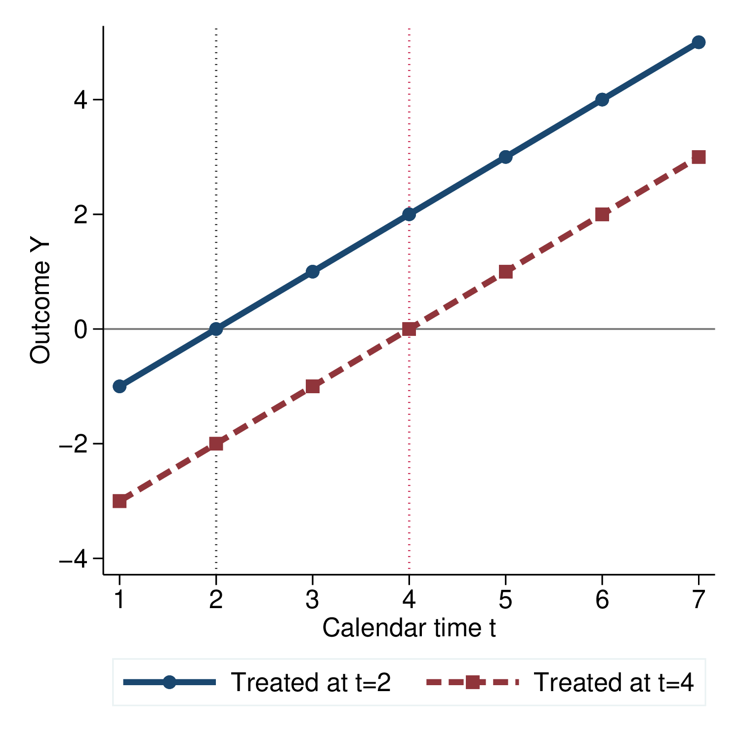
Figure 1: Underidentification of Fully-Dynamic Specification

Notes: This figure shows the evolution of outcomes over seven periods for two units (or cohorts), for the illustrative example of Section 3.2. Vertical lines mark the periods in which the two units are first treated.

The problem may be important in practice, as statistical packages may resolve this collinearity by dropping an arbitrary unit or period indicator. Some estimates of $\left\{\tau_{h}\right\}$ would then be produced, but because of an arbitrary trend in the coefficients they may suggest a violation of parallel trends even when the specification is in fact correct, i.e. Assumptions 1 and 2 hold and there is no heterogeneity of treatment effects for each horizon (Assumption 3).

To break the collinearity problem, stronger restrictions on anticipation effects, and thus on $Y_{it}$ for untreated observations, have to be introduced. One could consider imposing minimal restrictions on the specification that would make it identified. In typical cases, only a linear trend in $\left\{\tau_{h}\right\}$ is not identified in the fully dynamic specification, while nonlinear paths cannot be reproduced with unit and period fixed effects. Therefore, just one additional normalization, e.g. $\tau_{-a}=0$ in addition to $\tau_{-1}=0$, breaks multicollinearity.

However, minimal identified models rely on ad hoc identification assumptions which are a priori unattractive. For instance, just imposing $\tau_{-a}=\tau_{-1}=0$ means that anticipation effects are assumed away $1$ and $a$ periods before treatment, but not in other pre-periods. This assumption therefore depends on the realized event times. Instead, a systematic approach is to impose the assumptions — some forms of no anticipation effects and parallel trends — that the researcher has an a priori argument for and which motivated the use of DiD. Such assumptions also give much stronger identification power.

3.3 Negative Weighting in the Static Regression

We now show how, by imposing Assumption 3 instead of specifying the estimation target, the static TWFE specification does not identify a reasonably-weighted average of heterogeneous treatment effects: the underlying weights may be negative, particularly for the long-run causal effects. The issues we discuss here also arise in dynamic specifications that bin multiple lags together.

First, we note that, if the parallel-trends and no-anticipation assumptions hold, the static specification identifies some weighted average of treatment effects:

Proposition 2.

If Assumptions 1 and 2 hold, then the estimand of the static specification in Equation 3 satisfies $\tau^{\text{static}}=\sum_{it\in\Omega_{1}}w_{it}^{\text{static}}\tau_{it}$ for some weights $w_{it}^{\text{static}}$ that do not depend on the outcome realizations and add up to one, $\sum_{it\in\Omega_{1}}w_{it}^{\text{static}}=1$.

The underlying weights $w_{it}^{\text{static}}$ can be computed from the data using the Frisch–Waugh–Lovell theorem (see equation Equation 17 in the proof of Proposition 2) and only depend on the timing of treatment for each unit and the set of observed units and periods. The static specification’s estimand, however, cannot be interpreted as a proper weighted average, as some weights can be negative, which we illustrate with a simple example:

Proposition 3.

Suppose Assumptions 1 and 2 hold and the data consist of two units (or equal-sized cohorts), $A$ and $B$, treated in periods 2 and 3, respectively, both observed in periods $t=1,2,3$ (as shown in Table 1). Then the estimand of the static specification Equation 3 can be expressed as $\tau^{\text{static}}=\tau_{A2}+\frac{1}{2}\tau_{B3}-\frac{1}{2}\tau_{A3}$.

Table 1: Two-Unit, Three-Period Example

$\mathbb{E}\left[Y_{it}\right]$	$i=A$	$i=B$
$t=1$	$\alpha_{A}$	$\alpha_{B}$
$t=2$	$\alpha_{A}+\beta_{2}+\tau_{A2}$	$\alpha_{B}+\beta_{2}$
$t=3$	$\alpha_{A}+\beta_{3}+\tau_{A3}$	$\alpha_{B}+\beta_{3}+\tau_{B3}$
Event date	$E_{i}=2$	$E_{i}=3$

Notes: This table shows the evolution of expected outcomes over three periods for two units (or cohorts), for the illustrative example of Proposition 3. Without loss of generality, we normalize $\beta_{1}=0$.

This example illustrates the severe short-run bias of the static specification: the long-run causal effect, corresponding to the early-treated unit $A$ and the late period 3, enters with a negative weight ($-1/2$). Thus, larger long-run effects make the coefficient smaller.

This problem results from what we call “forbidden comparisons” performed by the static specification. Recall that the original idea of DiD estimation is to compare the evolution of outcomes over some time interval for the units which got treated during that interval relative to a reference group of units which didn’t, identifying the period FEs. In the Proposition 3 example, such an “admissible” comparison is between units $A$ and $B$ in periods 2 and 1, $\left(Y_{A2}-Y_{A1}\right)-\left(Y_{B2}-Y_{B1}\right)$. However, panels with staggered treatment timing also lend themselves to a second type of comparisons — which we label “forbidden” — in which the reference group has been treated throughout the relevant period. For units in this group, the treatment indicator $D_{it}$ does not change over the relevant period, and so the restrictive specification uses them to identify period FEs, too. The comparison between units $B$ and $A$ in periods 3 and 2, $\left(Y_{B3}-Y_{B2}\right)-\left(Y_{A3}-Y_{A2}\right)$, in Proposition 3 is a case in point. While a comparison like this is appropriate and increases efficiency when treatment effects are homogeneous (which the static specification was designed for), forbidden comparisons are problematic under treatment effect heterogeneity. For instance, subtracting $\left(Y_{A3}-Y_{A2}\right)$ not only removes the gap in period FEs, $\beta_{3}-\beta_{2}$, but also deducts the evolution of treatment effects $\tau_{A3}-\tau_{A2}$, placing a negative weight on $\tau_{A3}$. The restrictive specification leverages comparisons of both types and estimates the treatment effect by $\hat{\tau}^{static}=\left(Y_{B2}-Y_{A2}\right)-\frac{1}{2}\left(Y_{B1}-Y_{A1}\right)-\frac{1}{2}\left(Y_{B3}-Y_{A3}\right)$.

Fundamentally, this problem arises because the specification imposes very strong restrictions on treatment effect homogeneity, i.e. Assumption 3, instead of acknowledging the heterogeneity and specifying a particular target estimand (or perhaps a class of estimands that the researcher is indifferent between).

With a large number of never-treated units or a large number of periods before any unit is treated (relative to other units and periods), our setting becomes closer to a classical non-staggered DiD design, and therefore negative weights disappear, as our next result illustrates:

Proposition 4.

Suppose all units are observed for all periods $t=1,\dots,T$ and the earliest treatment happens at $E_{\text{first}}>1$. Let $N_{1}^{*}$ be the number of observations for never-treated units before period $E_{\text{first}}$ and $N_{0}^{*}$ be the number of untreated observations for ever-treated units since $E_{\text{first}}$. Then there is no negative weighting, i.e. $\min_{it\in\Omega_{1}}w_{it}^{\text{static}}\geq 0$, if and only if $N_{1}^{*}\geq N_{0}^{*}$.

Even when weights are non-negative, they may remain highly unequal and diverge from the estimands that the researcher is interested in. Our preferred strategy is therefore to commit to the estimation target and explicitly allow for treatment effect heterogeneity, except when some form of Assumption 3 is ex ante appropriate.

3.4 Spurious Identification of Long-Run Effects in Dynamic Specifications

Another consequence of inappropriately imposing Assumption 3 concerns estimation of long-run causal effects. Conventional dynamic specifications (except those subject to the underidentification problem) yield some estimates for all $\tau_{h}$ coefficients. Yet, for large enough $h$, no averages of treatment effects are identified under Assumptions 1 and 2 with unrestricted treatment effect heterogeneity. Therefore, estimates from restrictive specifications are fully driven by unwarranted extrapolation of treatment effects across observations and may not be reliable, unless strong ex ante reasons for Assumption 3 exist.

This issue is well illustrated in the example of Proposition 3. To identify the long-run effect $\tau_{A3}$ under Assumptions 1 and 2, one needs to form an admissible DiD comparison, of the outcome growth over some period between unit $A$ and another unit not yet treated in period 3. However, by period 3 both units have been treated. Mechanically, this problem arises because the period fixed effect $\beta_{3}$ is not identified separately from the treatment effects $\tau_{A3}$ and $\tau_{B3}$ in this example, absent restrictions on treatment effects. Yet, the semi-dynamic specification

$$Y_{it}=\tilde{\alpha}_{i}+\tilde{\beta}_{t}+\tau_{0}\mathbf{1}\left[K_{it}=0\right]+\tau_{1}\mathbf{1}\left[K_{it}=1\right]+\tilde{\varepsilon}_{it}$$

will produce an estimate $\hat{\tau}_{1}$ via extrapolation. Specifically, two different parameters, $\tau_{A3}-\tau_{B3}$ and $\tau_{A2}$, are identified by comparing the two units in periods 2 or 3, respectively, with period 1. Therefore, when imposing homogeneity of short-run effects across units, $\tau_{A2}=\tau_{B3}\equiv\tau_{0}$, we estimate the long-run effect $\tau_{A3}\equiv\tau_{1}$ as the sum of $\tau_{1}-\tau_{0}$ and $\tau_{0}$:

$$\hat{\tau}_{1}=\left[\left(Y_{A3}-Y_{A1}\right)-\left(Y_{B3}-Y_{B1}\right)\right]+\left[\left(Y_{A2}-Y_{A1}\right)-\left(Y_{B2}-Y_{B1}\right)\right].$$

However, when $\tau_{A2}\neq\tau_{B3}$, this estimator is biased.

In general, the gap between the earliest and the latest event times observed in the data provides an upper bound on the number of dynamic coefficients that can be identified without extrapolation of treatment effects. This result, which follows by the same logic of non-identification of the later period effects, is formalized by our next proposition:

Proposition 5.

Suppose there are no never-treated units and let $\bar{H}=\max_{i}E_{i}-\min_{i}E_{i}.$ Then, for any non-negative weights $w_{it}$ defined over the set of observations with $K_{it}\geq\bar{H}$ (that are not identically zero), the weighted sum of causal effects $\sum_{it\colon K_{it}\geq\bar{H}}w_{it}\tau_{it}$ is not identified by Assumptions 1 and 2.

Robust estimators, including the one we characterize in Section 4, can only be computed for identified estimands, never resulting in spurious estimates.

We finally note that the challenges described in Section 3 apply even if the sample is “trimmed” to a fixed window around the event time; see Section A.3.

4 Imputation-Based Estimation and Testing

To overcome the challenges affecting conventional practice, we now derive the robust and efficient estimator and show that it takes a particularly transparent “imputation” form when no restrictions on treatment-effect heterogeneity are imposed. We then perform asymptotic analysis, establishing the conditions for the estimator to be consistent and asymptotically normal, derive conservative standard error estimates for it, and discuss appropriate pre-trend tests.

Throughout, we continue to suppose that the researcher chose the estimation target $\tau_{w}$ and assumed a model of $Y_{it}(0)$ (Assumption 1^′) and no anticipation. Some model of treatment effects (Assumption 3) may also be assumed, although our main focus is on the null model, under which treatment effect heterogeneity is unrestricted. Letting $\varepsilon_{it}=Y_{it}-\mathbb{E}\left[Y_{it}\right]$ for $it\in\Omega$, we thus have under Assumptions 1^′, 2 and 3^′:

$$Y_{it}=A_{it}^{\prime}\lambda_{i}+X_{it}^{\prime}\delta+D_{it}\Gamma_{it}^{\prime}\theta+\varepsilon_{it}.$$ (4)

We assume throughout that $\tau_{w}=w_{1}^{\prime}\Gamma\theta$ is identified. Proposition A1 provides conditions for identification. First, we provide a general rank condition on the matrices of unit-specific and other covariates that requires that the covariate space of treated observations is spanned by that of the untreated ones. This assumption allows us to estimate from the untreated observations those nuisance parameters that are necessary to impute control outcomes of the treated observations, thus providing identification. Second, we derive specific conditions for the case where the parameter $\delta$ represents time fixed effects and $A_{it}$ may vary over time but not across units (as with unit FEs and unit-specific linear trends). In this case, we show that there is identification if (i) the $A_{it}$ are not collinear for any relevant unit and (ii) there is at least one untreated unit at the end of the time period of interest.

4.1 Efficient Estimation

For our efficiency result, we impose an additional assumption on the error variances:

Assumption 4 (Spherical errors).

Error terms $\varepsilon_{it}$ are spherical, i.e. homoskedastic and mutually uncorrelated across all $it\in\Omega$: $\mathbb{E}\left[\varepsilon\varepsilon^{\prime}\right]=\sigma^{2}\mathbb{I}_{N}$.

While this assumption is strong, our efficiency results also apply without change under dependence that is due to unit random effects, i.e. if $\varepsilon_{it}=\eta_{i}+\tilde{\varepsilon}_{it}$ for $\tilde{\varepsilon}_{it}$ that satisfy Assumption 4 and for some $\eta_{i}$. Moreover, these results are straightforward to relax to any known form of heteroskedasticity or mutual dependence. Under Assumption 4 and allowing for restrictions on causal effects, we have:

Theorem 1 (Efficient estimator).

Suppose Assumptions 1^′, 2, 3^′ and 4 hold. Then among the linear unbiased estimators of $\tau_{w}$, the (unique) efficient estimator $\hat{\tau}_{w}^{\ast}$ can be obtained with the following steps:

1. Estimate $\theta$ by the OLS solution $\hat{\theta}^{*}$ from the regression Equation 4 (where we assume that $\theta$ is identified);

2. Estimate the vector of treatment effects $\tau$ by $\hat{\tau}^{*}=\Gamma\hat{\theta}^{*}$;

3. Estimate the target $\tau_{w}$ by $\hat{\tau}_{w}^{\ast}=w_{1}^{\prime}\hat{\tau}^{*}$.

Moreover, this estimator $\hat{\tau}_{w}^{*}$ is unbiased for $\tau_{w}$ under Assumptions 1^′, 2 and 3^′ alone, even when error terms are not spherical.

Under Assumptions 1^′, 2 and 3^′, regression Equation 4 is correctly specified. Thus, this estimator for $\theta$ is unbiased by construction, and efficiency under spherical error terms is a direct consequence of the Gauss–Markov theorem. Moreover, OLS yields the most efficient estimator for any linear combination of $\theta$, including $\tau_{w}=w_{1}^{\prime}\Gamma\theta$. While assuming spherical errors may be unrealistic in practice, we think of this assumption as a natural conceptual benchmark to decide between the many unbiased estimators of $\tau_{w}$.

In the important special case of unrestricted treatment effect heterogeneity, $\hat{\tau}_{w}^{*}$ has a useful “imputation” representation. The idea is to estimate the model of $Y_{it}(0)$ using the untreated observations $it\in\Omega_{0}$ and leverage it to impute $Y_{it}(0)$ for treated observations $it\in\Omega_{1}$. Then, observation-specific causal effect estimates can be averaged appropriately. Perhaps surprisingly, the estimation and imputation steps are identical regardless of the target estimand. Applying any weights to the imputed causal effects yields the efficient estimator for the corresponding estimand. We have:

Theorem 2 (Imputation representation for the efficient estimator).

With a null Assumption 3^′ (that is, if $\Gamma=\mathbb{I}_{N_{1}}$), the unique efficient linear unbiased estimator $\hat{\tau}_{w}^{\ast}$ of $\tau_{w}$ from Theorem 1 can be obtained via an imputation procedure:

1. Within the untreated observations only ($it\in\Omega_{0}$), estimate the $\lambda_{i}$ and $\delta$ (by $\hat{\lambda}_{i}^{*},\hat{\delta}^{*}$) by OLS in

   $$Y_{it}=A_{it}^{\prime}\lambda_{i}+X_{it}^{\prime}\delta+\varepsilon_{it};$$ (5)

2. For each treated observation ($it\in\Omega_{1}$) with $w_{it}\neq 0$, set $\hat{Y}_{it}(0)=A_{it}^{\prime}\hat{\lambda}_{i}^{*}+X_{it}^{\prime}\hat{\delta}^{*}$ and $\hat{\tau}_{it}^{*}=Y_{it}-\hat{Y}_{it}(0)$ to obtain the estimate of $\tau_{it}$;

3. Estimate the target $\tau_{w}$ by a weighted sum $\hat{\tau}_{w}^{\ast}=\sum_{it\in\Omega_{1}}w_{it}\hat{\tau}_{it}^{*}$.

The imputation representation offers computational and conceptual benefits. First, it is computationally efficient as it only requires estimating a simple TWFE model, for which fast algorithms are available [54, 11]. This is in contrast to the OLS estimator from Theorem 1, as equation Equation 4 has regressors $\Gamma_{it}D_{it}$ in addition to the fixed effects, which are high-dimensional unless a low-dimensional model of treatment effect heterogeneity is imposed.

Second, the imputation approach is intuitive and transparently links the parallel trends and no-anticipation assumptions to the estimator. Indeed, [24] write: “At some level, all methods for causal inference can be viewed as imputation methods, although some more explicitly than others” (p. 141). We formalize this statement in the next proposition, which shows that any estimator unbiased for $\tau_{w}$ can be represented in the imputation way, but the way of imputing the $Y_{it}(0)$ may be less explicit and no longer efficient.

Proposition 6 (Imputation representation for all unbiased estimators).

Under Assumptions 1^′ and 2, any linear estimator $\hat{\tau}_{w}$ of $\tau_{w}$ that is unbiased under arbitrary treatment-effect heterogeneity (that is, a null Assumption 3) can be obtained via imputation:

1. For every treated observation, estimate expected untreated potential outcomes $A_{it}^{\prime}\lambda_{i}+X_{it}^{\prime}\delta$ by some unbiased linear estimator $\hat{Y}_{it}(0)$ using data from the untreated observations only;

2. For each treated observation, set $\hat{\tau}_{it}=Y_{it}-\hat{Y}_{it}(0)$;

3. Estimate the target by a weighted sum $\hat{\tau}_{w}=\sum_{it\in\Omega_{1}}w_{it}\hat{\tau}_{it}$.

This result establishes an imputation representation when treatment effects can vary arbitrarily. Proposition A2 in the appendix establishes that the imputation structure applies even when restrictions $\tau=\Gamma\theta$ are imposed, albeit with an additional step in which the weights $w_{1}$ defining the estimand are adjusted in a way that does not change $\tau_{w}$ under the imposed model. In this sense, unbiased causal inference is equivalent to imputation in our framework.

4.2 Asymptotic Properties

Having derived the linear unbiased estimator $\hat{\tau}_{w}^{\ast}$ for $\tau_{w}$ in Theorem 1 that is also efficient under spherical error terms, we now consider its asymptotic properties without imposing that assumption. We study convergence along a sequence of panels indexed by the sample size $N$, where randomness stems from the error terms $\varepsilon_{it}$ only, as in Section 2. Our approach applies to asymptotic sequences where both the number of units and the number of time periods may grow, but the assumptions are least restrictive when the number of time periods remains constant or grows slowly, as in short panels.

Instead of assuming that error terms are spherical, we now assume that error terms are clustered by units $i$.

Assumption 5 (Clustered error terms).

Error terms $\varepsilon_{it}$ are independent across units $i$ and have bounded variance, $\mathrm{Var}\left[\varepsilon_{it}\right]\leq\bar{\sigma}^{2}$ for $it\in\Omega$ uniformly.

The key role in our results is played by the weights that the Theorem 1 estimator places on each observation. Since the estimator is linear in the observed outcomes $Y_{it}$, we can write it as $\hat{\tau}_{w}^{*}=\sum_{it\in\Omega}v_{it}^{*}Y_{it}$ with non-stochastic weights $v_{it}^{*}$, derived in Proposition A3 in the appendix.

We now formulate high-level conditions on the sequence of weight vectors that ensure consistency, asymptotic normality, and will later allow us to provide valid inference. These results apply to any unbiased linear estimator $\hat{\tau}_{w}=\sum_{it\in\Omega}v_{it}Y_{it}$ of $\tau_{w}$, not just the efficient estimator $\hat{\tau}_{w}^{*}$ from Theorem 1 – that is, if the respective conditions are fulfilled for the weights $v_{it}$, then consistency, asymptotic normality, and valid inference follow as stated. For the specific estimator $\hat{\tau}_{w}^{*}$ introduced above, we then provide sufficient low-level conditions for short panels.

First, we obtain consistency of $\hat{\tau}_{w}$ under a Herfindahl condition on the weights $v$ that takes the clustering structure of error terms into account.

Assumption 6 (Herfindahl condition).

Along the asymptotic sequence, $\|v\|_{\textnormal{H}}^{2}\equiv\sum_{i}\left(\sum_{t;it\in\Omega}\left|v_{it}\right|\right)^{2}\rightarrow 0$, for weights $v_{it}$ in the unbiased linear estimator $\hat{\tau}_{w}=\sum_{it\in\Omega}v_{it}Y_{it}$.

The condition on the clustered Herfindahl index $\|v\|_{\textnormal{H}}^{2}$ states that the sum of squared weights vanishes, where weights are aggregated by units. One can think of the inverse of the sum of squared weights, $n_{H}=\|v\|_{\textnormal{H}}^{-2}$, as a measure of effective sample size, which Assumption 6 requires to grow large along the asymptotic sequence. If it is satisfied, and variances are uniformly bounded, we obtain consistency of $\hat{\tau}_{w}$:

Proposition 7 (Consistency of $\hat{\tau}_{w}$).

Under Assumptions 1^′, 2, 3^′, 5 and 6, $\hat{\tau}_{w}-\tau_{w}\stackrel{{\scriptstyle\mathcal{L}_{2}}}{{\rightarrow}}0$ for an unbiased linear estimator $\hat{\tau}_{w}$ of $\tau_{w}$, such as $\hat{\tau}_{w}^{*}$ in Theorem 1.

We note that the large number of unit-specific parameters $\left\{\lambda_{i}\right\}_{i}$ cannot generally be estimated consistently in panels with a small number of time periods, raising a potential incidental-parameters problem. However, consistency of $\hat{\tau}_{w}$ does not rely on consistency for unit-specific parameters, since our estimator averages over many units.

We next consider the asymptotic distribution of the estimator around the estimand.

Proposition 8 (Asymptotic normality).

If the assumptions of Proposition 7 hold, there exists $\kappa>0$ such that $\mathbb{E}\left[\left|\varepsilon_{it}\right|^{2+\kappa}\right]$ is uniformly bounded, the weights are not too concentrated in the sense that $\sum_{i}\left(\sqrt{n_{H}}\sum_{t;it\in\Omega}\left|v_{it}\right|\right)^{2+\kappa}\rightarrow 0$, and the variance does not vanish, $\liminf n_{H}\sigma_{w}^{2}>0$ for $\sigma_{w}^{2}=\mathrm{Var}\left[\hat{\tau}_{w}\right]$, then we have that $\sigma_{w}^{-1}(\hat{\tau}_{w}-\tau_{w})\stackrel{{\scriptstyle d}}{{\rightarrow}}\mathcal{N}(0,1)$.

This result establishes conditions under which the difference between estimator and estimand is asymptotically normal. Besides regularity, this proposition requires that the estimator variance $\sigma_{w}^{2}$ does not decline faster than $1/n_{H}$. It is violated if the clustered Herfindahl formula is too conservative: for instance, if the number of periods is growing along the asymptotic sequence while the within-unit over-time correlation of error terms remains small. Alternative sufficient conditions for asymptotic normality can be established in such cases, e.g. along the lines of Footnote 24.

So far, we have formulated high-level conditions on the weights $v_{it}$ of any linear unbiased estimator of $\tau_{w}$. Section A.7 presents low-level sufficient conditions for consistency and asymptotic normality of the imputation estimator $\hat{\tau}_{w}^{*}$ for the benchmark case of a panel with unit and period FEs, a fixed or slowly growing number of periods, and no restrictions on treatment effects. Unlike Propositions 7 and 8, these conditions are imposed directly on the weights $w_{1}$ chosen by the researcher, and not on the the implied weights $v_{it}^{\ast}$, such that the researcher can assess more directly whether the asymptotic approximation is likely to be precise. In particular, the estimator achieves consistency and asymptotic normality in the common case where the number of time periods is fixed, the size of all cohorts increases, the weights on treatment effects do not vary within the same period and cohort, and the sum of (absolute) weights is bounded. In addition, the sufficient conditions are also fulfilled when the number of periods grows slowly and when weights differ across observations within the same cohort and period, but not by too much. With covariates other than unit and period FEs, e.g. with unit-specific linear trends, the general weight conditions in Assumption 6 and Proposition 8 can also be used to verify consistency and asymptotic normality. In those cases, the sufficient conditions are typically fulfilled for convex combinations of cohort-average treatment effects whenever the size of cohorts grows sufficiently fast relatively to the number of periods (see Section A.7).

4.3 Conservative Inference

We next estimate the variance of $\hat{\tau}_{w}=\sum_{it\in\Omega}v_{it}Y_{it}$, which equals $\sigma_{w}^{2}=\mathbb{E}\left[\sum_{i}\left(\sum_{t;it\in\Omega}v_{it}\varepsilon_{it}\right)^{2}\right]$ with clustered error terms (Assumption 5). We start with the case where treatment effect heterogeneity is unrestricted (i.e. $\Gamma=\mathbb{I}$). As in [51], exact inference becomes infeasible when treatment effects are heterogeneous, but conservative inference is possible. Following Section 4.2, the inference tools we propose apply to a generic linear unbiased estimator but we use them for the efficient estimator $\hat{\tau}_{w}^{\ast}$. Our strategy is to estimate individual error terms by some $\tilde{\varepsilon}_{it}$ and then use a plug-in estimator,

$$\hat{\sigma}_{w}^{2} =\sum_{i}\left(\sum_{t;it\in\Omega}v_{it}\tilde{\varepsilon}_{it}\right)^{2}.$$ (6)

Estimating the error terms presents two challenges, which become apparent when we consider the benchmark choice $\tilde{\varepsilon}_{it}=\hat{\varepsilon}_{it}$ based on the regression residuals $\hat{\varepsilon}_{it}=Y_{it}-A_{it}^{\prime}\hat{\lambda}_{i}^{*}-X_{it}^{\prime}\hat{\delta}^{*}-D_{it}\hat{\tau}_{it}^{*}$ in the regression Equation 4. The first challenge is the incidental-parameters problem in estimating $\lambda_{i}$. However, by using cluster-robust variance estimates, our inference does not suffer from this problem since the variance estimator $\hat{\sigma}_{w}^{2}$ does not rely on the consistent estimation of $\lambda_{i}$ any more, similar to the insight of [42].

A second challenge arises from unrestricted treatment-effect heterogeneity. In Theorem 2, treatment effects are estimated by fitting the corresponding outcomes $Y_{it}$ perfectly, with residuals $\hat{\varepsilon}_{it}\equiv 0$ for all treated observations. This issue is not specific to our estimation procedure: one generally cannot distinguish between $\tau_{it}$ and $\varepsilon_{it}$ from observations of $Y_{it}=A_{i}^{\prime}\lambda_{i}+X_{it}^{\prime}\delta+\tau_{it}+\varepsilon_{it}$ for treated observations, making it impossible to produce unbiased estimates of $\sigma_{w}^{2}$ (see Lemma 1 in [56] for a similar impossibility result).

While unbiased estimation of $\sigma_{w}^{2}$ is not possible, we show that this variance can be estimated conservatively. Our variance estimator is based on an auxiliary parsimonious model of treatment effects. We do not require this model to be correct, in the sense that inference is weakly asymptotically conservative under misspecification. However, auxiliary models which better approximate $\tau_{it}$ will make confidence intervals tighter and closer to asymptotically exact. In the computation of $\hat{\sigma}_{w}^{2}$ we set $\tilde{\varepsilon}_{it}$ for the treated observations equal to the residuals of the auxiliary model. We require the model to be parsimonious, such that it does not overfit and the residuals include $\varepsilon_{it}$. When the model is incorrect, $\tilde{\varepsilon}_{it}$ also include a component due to the misspecification of $\tau_{it}$, leading to conservative inference.

We formalize the auxiliary model by considering estimators $\tilde{\tau}_{it}$ for each $it\in\Omega_{1}$ which satisfy two properties: (1) $\tilde{\tau}_{it}$ converges to some non-stochastic limit $\bar{\tau}_{it}$ and (2) if the auxiliary model is correct, $\bar{\tau}_{it}=\tau_{it}$. The following theorem presents conditions under which our construction yields asymptotically conservative inference:

Theorem 3 (Conservative clustered standard error estimates).

Assume that the assumptions of Proposition 7 hold, that the model of treatment effects is trivial ($\Gamma=\mathbb{I}$), that the estimates $\tilde{\tau}_{it}$ converge to some non-random $\bar{\tau}_{it}$ in the sense that $\|v\|_{\textnormal{H}}^{-2}\sum_{i}\left(\sum_{t;it\in\Omega_{1}}v_{it}(\tilde{\tau}_{it}-\bar{\tau}_{it})\right)^{2}\stackrel{{\scriptstyle p}}{{\rightarrow}}0$, that $\hat{\delta}^{*}$ from Theorem 1 is sufficiently close to $\delta$ in the sense that $\|v\|_{\textnormal{H}}^{-2}\sum_{i}\left(\sum_{t;it\in\Omega}v_{it}X_{it}^{\prime}(\hat{\delta}^{\ast}-\delta)\right)^{2}\stackrel{{\scriptstyle p}}{{\rightarrow}}0$, and that $\left|\tau_{it}\right|,$ $\left|\bar{\tau}_{it}\right|$ and $\mathbb{E}\left[\varepsilon_{it}^{4}\right]$ are uniformly bounded and the weights are not too concentrated in the sense that $\sum_{i}\left(\frac{\sum_{t;it\in\Omega}\lvert v_{it}\rvert}{\|v\|_{\textnormal{H}}}\right)^{4}\rightarrow 0$. Then the variance estimate

$$\hat{\sigma}_{w}^{2} =\sum_{i}\left(\sum_{t;it\in\Omega}v_{it}\tilde{\varepsilon}_{it}\right)^{2}, \tilde{\varepsilon}_{it} =Y_{it}-A_{it}^{\prime}\hat{\lambda}_{i}^{*}-X_{it}^{\prime}\hat{\delta}^{*}-D_{it}\tilde{\tau}_{it}$$ (7)

is asymptotically conservative: $\|v\|_{\textnormal{H}}^{-2}(\hat{\sigma}_{w}^{2}-\sigma_{w}^{2}-\sigma_{\tau}^{2})\stackrel{{\scriptstyle p}}{{\rightarrow}}0$ where $\sigma_{\tau}^{2}=\sum_{i}\left(\sum_{t;D_{it}=1}v_{it}(\tau_{it}-\bar{\tau}_{it})\right)^{2}\geq 0$. If $\bar{\tau}_{it}=\tau_{it}$ for all $it\in\Omega_{1}$, $\sigma_{\tau}^{2}=0$, meaning that the variance estimate is asymptotically exact.

The theorem shows that the proposed variance estimate addresses the two challenges laid out above. First, the estimates remain valid even though we may not be able to estimate the unit-specific parameters $\lambda_{i}$ consistently. This is because unit-specific parameter estimates drop out when summing over all observations of one unit in Equation 7, as shown in the proof. Second, by using estimates $\tilde{\tau}_{it}$ that fulfill the convergence condition of the theorem, we avoid the issue of obtaining trivial residuals for the treated observations. The resulting variance estimates are asymptotically conservative. From these estimates we can also obtain conservative confidence intervals (that asymptotically have coverage that is at least nominal) if the estimator is also asymptotically normal, such as under the sufficient conditions of Proposition 8.

It remains to choose the estimates $\tilde{\tau}_{it}$. We focus on auxiliary models that impose the equality of treatment effects across large groups of treated observations: for a partition $\Omega_{1}=\bigcup_{g}G_{g}$, $\tau_{it}\equiv\tau_{g}$ for all $it\in G_{g}$. The $\tau_{g}$ can then be estimated by some weighted average of $\hat{\tau}_{it}^{*}$ among $it\in G_{g}$. Specifically, we propose averages of the form

$$\tilde{\tau}_{g}=\frac{\sum_{i}\left(\sum_{t;it\in G_{g}}v_{it}\right)\left(\sum_{t;it\in G_{g}}v_{it}\hat{\tau}_{it}^{*}\right)}{\sum_{i}\left(\sum_{t;it\in G_{g}}v_{it}\right)^{2}}.$$ (8)

In Section A.8, we show that this choice of weights leads to minimal excess variance $\sigma_{\tau}^{2}$ in the case where there is only a single group $g$, corresponding to a conservative auxiliary model which requires all treatment effects to be the same. The choice of the partition aims to maintain a balance between avoiding overly conservative variance estimates and ensuring consistency. If the sample is large enough, one may want to partition $\Omega_{1}$ into multiple groups of observations such that treatment effect heterogeneity is expected to be smaller within them than across. For instance, with many units, a group may consist of observations corresponding to the same horizon relative to treatment onset. If cohorts are large, one can further partition observations into groups defined by cohort and period, which we use as the default in our Stata command.

While sufficiently large groups in Equation 8 avoid overfitting asymptotically (under appropriate conditions), in finite samples these $\tilde{\tau}_{it}$ still use $\hat{\tau}_{it}^{*}$ and thus partially overfit to $\varepsilon_{it}$. In Section A.9 we therefore also consider leave-out versions of these $\tilde{\tau}_{it}$.

We make four final remarks on Theorem 3. First, our strategy for estimating the variance extends directly to conservative estimation of variance-covariance matrices for vector-valued estimands, e.g. for average treatment effects at multiple horizons $h$. Second, the result applies in short panels under the low-level conditions of Section A.7 (see Proposition A7). Third, while we have focused here on the case of unrestricted heterogeneity ($\Gamma=\mathbb{I}$), Theorem 3 can be extended to the case with a non-trivial treatment-effect model imposed in Assumption 3. Finally, computation of $\hat{\sigma}_{w}^{2}$ for the estimator $\hat{\tau}_{w}^{*}$ from Theorem 1 involves the implied weights $v_{it}^{*}$, which becomes computationally challenging with multiple sets of high-dimensional FEs. In Section A.10 we develop a computationally efficient algorithm for computing $v_{it}^{*}$ based on the iterative least squares algorithm for conventional regression coefficients [54].

4.4 Testing for Parallel Trends

In this section, we discuss testing the (generalized) parallel-trend and no-anticipation assumptions Assumptions 1^′ and 2. We propose a testing procedure based on OLS regressions with untreated observations only, departing from both traditional regression-based tests and more recent placebo tests. This procedure is robust to treatment effect heterogeneity and, under spherical errors, has attractive power properties and avoids the problem of inference after pre-testing explained by [37]. We propose:

Test 1.

(Robust OLS-based pre-trend test)

1. Choose an alternative model for $Y_{it}$ for untreated observations $it\in\Omega_{0}$ that is richer than that imposed by Assumptions 1^′ and 2: for an observable vector $W_{it}$ (which we consider non-stochastic, like $A_{it}$ and $X_{it}$),

   $$Y_{it}=A_{it}^{\prime}\lambda_{i}+X_{it}^{\prime}\delta+W_{it}^{\prime}\gamma+\varepsilon_{it};$$ (9)

2. Estimate $\gamma$ by $\hat{\gamma}$ in Equation 9 using OLS on untreated observations only;

3. Test $\gamma=0$ using the heteroskedasticity- and cluster-robust Wald test.

This test is valid because equation Equation 9 is implied by Assumptions 1^′ and 2 if the null $\gamma=0$ holds.

The test requires choosing $W_{it}$ to parametrize the possible violation of Assumptions 1^′ and 2. A natural choice for $W_{it}$, which parallels conventional pre-trend tests, is a set of indicators for observations $1,\dots,k$ periods before the onset of treatment for some $k$, with periods before $E_{i}-k$ serving as the reference group. This choice is appropriate, for instance, if the researcher’s main worry is the possible effects of treatment anticipation, i.e. violations of Assumption 2. This choice of $W_{it}$ also lends itself to making “event study plots,” which combine the ATT estimates by horizon $h\geq 0$ with a series of pre-trend coefficients; we supply the event_plot Stata command for this goal. Alternatively, the researcher may focus on possible violations of Assumption 1^′. For instance, with data spanning many years one could test for the presence of a structural break in unit FEs.

Test 1 can be contrasted with two existing strategies to test parallel trends. Traditionally, researchers estimated a dynamic specification including lags and leads of treatment onset, and tested — visually or statistically — that the coefficients on leads are equal to zero. More recent papers [[, e.g.]]DeChaisemartin2018,Liu2020a replace it with a placebo strategy: pretend that treatment happened $k$ periods earlier for all eventually treated units, and estimate the average effects $h=0,\dots,k-1$ periods after the placebo treatment using the same estimator as for actual estimation.

Both of these alternatives strategies have drawbacks. Because the traditional regression-based test uses the full sample, including treated observations, and imposes restrictions on treatment effects (which are assumed homogeneous within each horizon), it is not a test for Assumptions 1^′ and 2 only. Rather, it is a joint test that is sensitive to violations of the implicit Assumption 3 [60]. Even if a researcher has reasons to impose a non-trivial Assumption 3 in estimation, a robust test for parallel trends and no anticipation per se should avoid those restrictions on treatment effect heterogeneity. With a null Assumption 3, treated observations are not useful for testing, and our test only uses the untreated ones.

Tests based on placebo estimates appropriately use untreated observations only and may have intuitive appeal. However, mimicking the estimator does not generally correspond to an efficient test of a class of plausible alternatives. In contrast, Test 1 possesses well-known asymptotic efficiency properties when $W_{it}$ is correctly specified. For example, when $\varepsilon_{it}$ are spherical and normal, it is asymptotically equivalent to the homoskedastic $F$-test, which is a uniformly most powerful invariant test [30, ch. 7.6].

Finally, we show an additional advantage of Test 1: if the researcher conditions on the test passing (i.e. does not report the results otherwise), inference on $\hat{\tau}_{w}^{\ast}$ is still asymptotically valid under the null of no violations of Assumptions 1^′ and 2 and under spherical errors. This avoids the issue pointed out by [37, Proposition 4] in the context of restrictive dynamic event study regressions: that variance estimates which do not take pre-testing into account are inflated, leading to unnecessarily conservative inference.

Proposition 9 (Pre-test robustness).

Suppose the model in Equation 9 and Assumption 4 hold. Then $\hat{\tau}_{w}^{\ast}$ constructed as in Theorem 1 is uncorrelated with any vector $\hat{\gamma}$ constructed as in Test 1. If the error terms are also normally distributed, then $\hat{\tau}_{w}^{\ast}$ and $\hat{\gamma}$ are independent, and inference on $\tau_{w}$ based on $\hat{\tau}_{w}^{\ast}$ is unaffected by pre-tests based on $\hat{\gamma}$.

5 Application

Having derived the attractive theoretical properties of the imputation estimator, we now illustrate their practical relevance by revisiting the estimation of the marginal propensity to spend in the event study of [7]. We also use this empirical setting to verify the properties of the imputation estimator in a simulation study.

5.1 Setting

The marginal propensity to spend out of tax rebates is a crucial parameter for economic policy. In the US, the Economic Stimulus Act of 2008 consisted primarily of a 100 billion dollar program that sent tax rebates to approximately 130 million tax filers. [35] and [7] estimate the marginal propensity to spend (MPX) out of the 2008 tax rebates. The rebate was disbursed using two methods: either via direct deposit to a bank account, if known by the IRS, or with a mailed paper check. For each method, the week in which the funds were disbursed depended on the second-to-last digit of the taxpayer’s Social Security number (SSN). This number provides a source of quasi-experimental variation because the last four digits of a SSN are assigned sequentially to applicants within geographic areas.

[7, henceforth BP] use an event study design to examine the response of nondurable spending to tax rebate receipt, leveraging the quasi-experimental variation in the timing of the receipt. The quasi-random assignment of the last digits of the SSN makes the parallel-trends assumption for expenditures a priori plausible. The no-anticipation assumption may also be expected to hold: although the disbursement schedule was known in advance, households were directly notified by mail only several days before disbursement.

We estimate the performance of various estimators at estimating the impulse response function of nondurable spending to tax rebate receipt using the same data as BP. While earlier work by [35] estimates the impulse responses using quarterly spending data from the Consumer Expenditure Survey, BP leverage more detailed data from the Nielsen Homescan Consumer Panel. The Nielsen dataset tracks transactions at a much higher (in principle, daily) frequency, which is why we choose it for our analysis. The Nielsen data cover expenditures on consumer packaged goods (food, beverages, beauty and health products, household supplies, and general merchandise), representing around 15% of total household expenditures. Our dataset, identical to that of BP, is a complete panel of 21,760 households (including 21,690 with non-missing disbursement method information) observed over 52 weeks of year 2008.

5.2 Comparison between Robust and Conventional Estimates

We show how BP’s estimates of the MPX suffer from an upward bias in the short-run due to the choice of a binned specification (Section 5.2.1) and how they may be spurious in the long-run (Section 5.2.2). In Section 5.2.3 we present our preferred robust estimates and discuss implications for the macroeconomics literature.

5.2.1 Negative Weighting and Upward Bias with Binning

We replicate BP’s estimates, focusing on the first three months since the receipt, while leaving longer-run effects to Section 5.2.2. BP estimate conventional dynamic specifications of the form:

$$Y_{it}=\alpha_{i}+\beta_{t}+\sum_{h=-a}^{b}\tau_{h}\mathbf{1}\left[K_{it}=h\right]+\varepsilon_{it},$$ (10)

where $Y_{it}$ is the dollar amount of spending in calendar week $t$ for household $i$, $\alpha_{i}$ are household FEs, and $\beta_{t}$ are week FEs. In some specifications, week FEs are interacted with the disbursement method $m(i)$ (i.e., $\beta_{m(i)t}$ is included instead of $\beta_{t}$ in Equation 10) to leverage the variation in timing only within each disbursement method; we refer to those specifications as “with disbursement method FEs.” The set of $\mathbf{1}\left[K_{it}=h\right]$ are the lead/lag indicator variables tracking the number of weeks $K_{it}=t-E_{i}$ since the week of the tax rebate receipt for the household, $E_{i}$; $b$ is chosen such that all possible lags in the sample are covered; $a$ varies as discussed below. MPXs for each horizon, as well as pre-trend coefficients, are captured by $\tau_{h}$. Regressions are weighted by the Nielsen projection weights.

BP’s preferred specification is a binned version of Equation 10 which constrains $\tau_{h}$ to be constant across four-week periods — “months” — around the event, starting with the week of tax rebate receipt: e.g., $\tau_{0}=\dots=\tau_{3}$. This specification also includes one monthly pre-trend coefficient, i.e. $a=4$ with $\tau_{-1}=\dots=\tau_{-4}.$ These estimates, without and with disbursement method FEs, are replicated in Table 2, columns 1 and 2, suggesting that tax rebate receipt led to an increase in spending in the contemporaneous month of $42.6 (s.e. 7.2) in col. 1 to $47.6 (s.e. 9.2) in col. 2, and a cumulative increase over three months of $60.5 (s.e. 25.7) in col. 1 to $94.4 (s.e. 33.5) in col. 2. As we will discuss in Section 5.2.3, extrapolating these estimates from Nielsen products to all consumption implies very large total MPX.

Table 2: Estimates of the Monthly and Quarterly MPX out of Tax Rebates

	Dollars spent after tax rebate receipt
	OLS			OLS			Imputation
	Monthly binned			No binning			Estimator
	(1)	(2)		(3)	(4)		(5)	(6)
Contemporaneous month	42.59	47.57		35.02	27.88		38.13	30.54
	(7.19)	(9.15)		(5.75)	(7.75)		(5.68)	(9.08)
First month after	9.31	26.26		$-2.28$	$-4.48$		–2.47	7.43
	(9.00)	(11.95)		(7.59)	(12.48)		(7.81)	(16.17)
Second month after	8.63	20.52		$-5.96$	$-13.82$		13.08	4.01
	(11.17)	(14.57)		(10.06)	(16.38)		(22.51)	(29.89)
Three-month total	60.53	94.35		26.79	9.58		48.75	41.97
	(25.73)	(33.54)		(21.43)	(34.42)		(30.97)	(46.56)
Disbursement method FE	No	Yes		No	Yes		No	Yes
N observations	1,131,520	1,127,880		1,131,520	1,127,880		631,040	536,553
N households	21,760	21,690		21,760	21,690		21,760	21,690

Notes: Columns 1 and 2 estimate the binned version of specification Equation 10 with $a=4$ and imposing that the coefficients are the same in each month, i.e. four weeks since the rebate receipt. Columns 3 and 4 estimate the same specification without binning, with $a=1$. These specifications are identical to [7], Tables 3 and 4, columns 1 and 4. Columns 5 and 6 report the efficient imputation estimator. All columns aggregate coefficients by month for the first three months after the rebate receipt and suppress the other coefficients. Columns 1, 3, and 5 use household and week FEs, while columns 2, 4, and 6 additionally interact week FEs with disbursement method dummies. The estimates in column 6 exclude the last week of the quarter ($h=11$) due to insufficient sample size. All estimates use projection weights from the Nielsen Consumer Panel, and standard errors are clustered by household.

Next, we show that the MPX estimates are much smaller without binning. In columns 3 and 4 of Table 2 we report the estimates from the conventional specification Equation 10 without binning and with one weekly lead ($a=1$), as in BP’s Table 3. We report the coefficients aggregated to the monthly level. Compared to columns 1 and 2, there is a large fall in the cumulative three-month MPX, from $60.5 (s.e. 25.7) to $26.8 (s.e. 21.4) without disbursement method FEs and from $94.4 (s.e. 33.5) to $9.6 (s.e. 34.4) with these FEs. In columns 5 and 6, we use the robust and efficient imputation estimator to estimate weekly average responses and aggregate them to the monthly level. The point estimates are similar to columns 3 and 4 for the contemporaneous month response, while for the quarterly MPX they are in between the results obtained with a binned specification and without binning.

Could the difference between binned and other estimates indicate a violation of the DiD assumptions? Figure 2 provides evidence against this possibility, showing that there is no sign of pre-trends. The Wald test confirms this finding: the p-value for the null of no pre-trends is 0.185 (0.403) without (with) disbursement method FEs.

Figure 2: Dynamic Specifications and Pre-Trends

A: Without disbursement method FEs		B: With disbursement method FEs

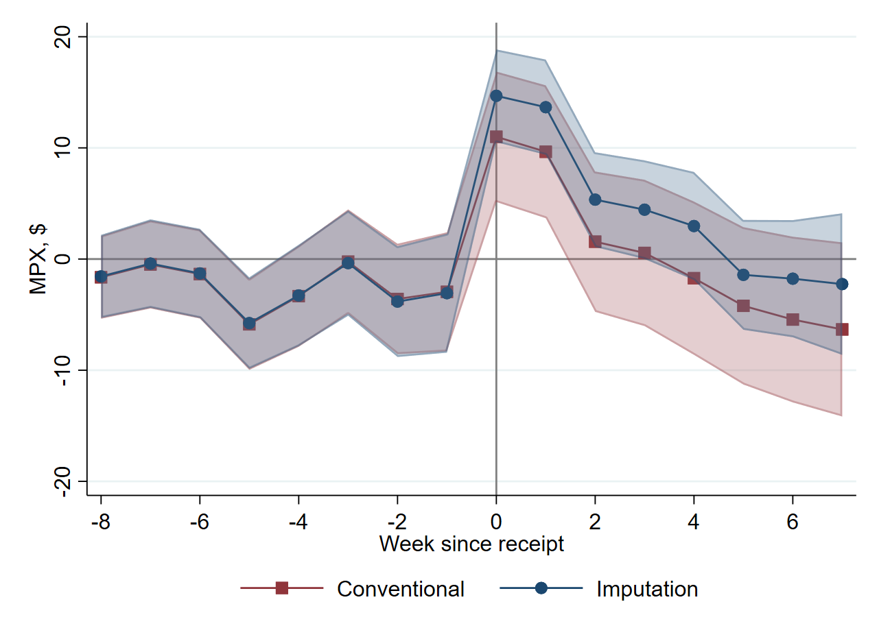
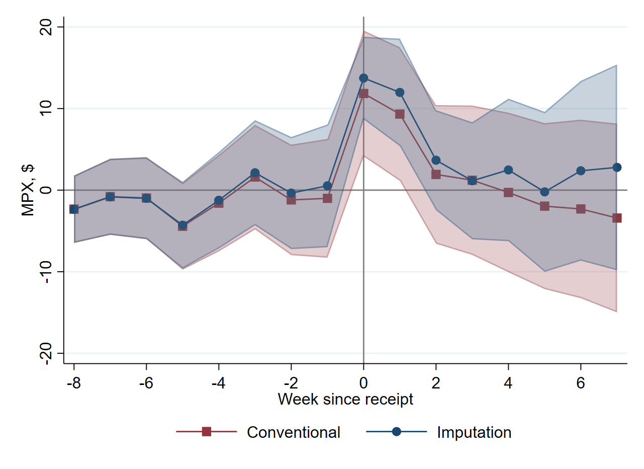
Notes: Panel A reports estimates of the response of spending to tax rebate receipts and pre-trend coefficients, using specification Equation 10 with $a=8$ and without binning (“Conventional”) and with the efficient imputation estimator and the pre-trend test from Section 4.4 (“Imputation”). Panel B additionally interacts week FEs with the disbursement method. Observations 8 or more weeks since the rebate receipt are excluded. Estimation is weighted by the projection weights from the Nielsen Consumer Panel. 95% confidence bands are shown, using standard errors clustered by household.

We find instead that the higher estimates from binned specifications are explained by the estimand they implicitly choose. Specifically, this estimand places a very large weight on the first weeks after the rebate, when the effects are the largest, and negative weights on other weeks. Figure 2 shows that the increase in spending after the receipt is concentrated in the first weeks since the rebate. Figure 3 in turn shows the weights with which the quarterly MPX estimated from the monthly binned specification of Table 2 aggregates the MPXs at each weekly horizon. These weights show how the estimand of the binned specification diverges from the true quarterly MPX, which is a simple sum of the effects at each horizon $h=0,\dots,11$ weeks, i.e. with constant weights of one on each week. In the specification without disbursement method FEs, the weight placed on the first-week response is three times larger than it would be with an equally weighted sum; it is five times larger with the FEs. Furthermore, within each month the weights become negative for the last weeks of the month. Applying the weights of the binned specification across weeks from Figure 2 to the estimates without binning (underlying col. 3 of Table 2), we obtain a point estimate of $42.6 for the contemporaneous month — indistinguishable from col. 1, instead of $35.0 in col. 3. Similarly, we get $60.4 for the quarter, nearly identical to $60.5 in col. 1, instead of $26.8 in col. 3. Thus, the short-run biased weighting scheme due to binning explains nearly all the difference between columns 1 and 3 of Table 2.

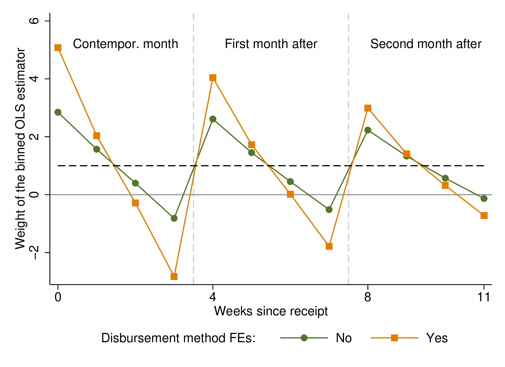
Figure 3: Short-term Bias in Weights for Binned Specifications

Notes: This figure reports the cumulative weight that the monthly binned OLS estimator of the quarterly MPX from Table 2, with or without disbursement methods FEs, places on the true effects at each horizon $h=0,\dots,11$ weeks since the rebate receipt. These weights are computed using the Frisch–Waugh–Lovell theorem, analogously to equation Equation 17, and aggregated across the first three months since the rebate receipt. The black dashed line indicates the weight corresponding to the true quarterly MPX, i.e. a simple sum of the effects at each horizon.

5.2.2 Spurious Identification of Long-Run Causal Effects

We now examine the long-run dynamics of MPXs obtained with conventional specifications and the imputation estimator. The timing of the tax rebate is such that we simultaneously observe treated and untreated households for at most 13 weeks. Per Proposition 5, without restrictive assumptions on treatment effect heterogeneity it is not possible to estimate causal effects beyond 12 weeks. Yet conventional dynamic specifications produce estimates for longer horizons via extrapolation. We examine whether the estimates obtained in this way could paint a misleading picture of the long-run dynamics of MPXs.

Figure 4: Long-run MPXs, Conventional Specifications vs. Robust Imputation Estimator

A: Conventional	B: Conventional	C: Robust
Binned Estimates	Dynamic Estimates	Imputation Estimates

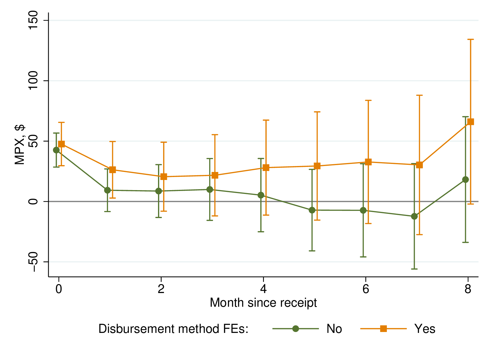
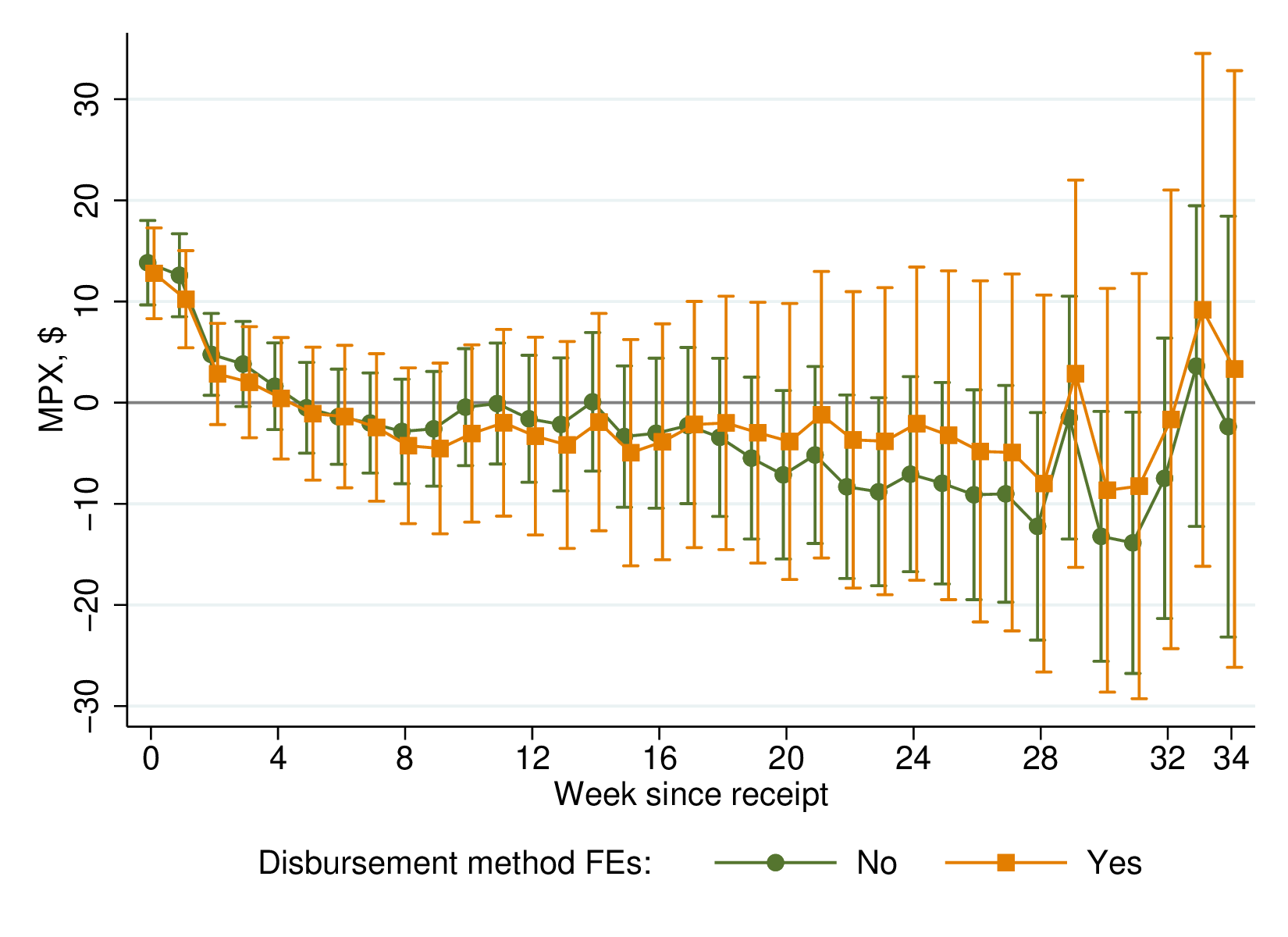
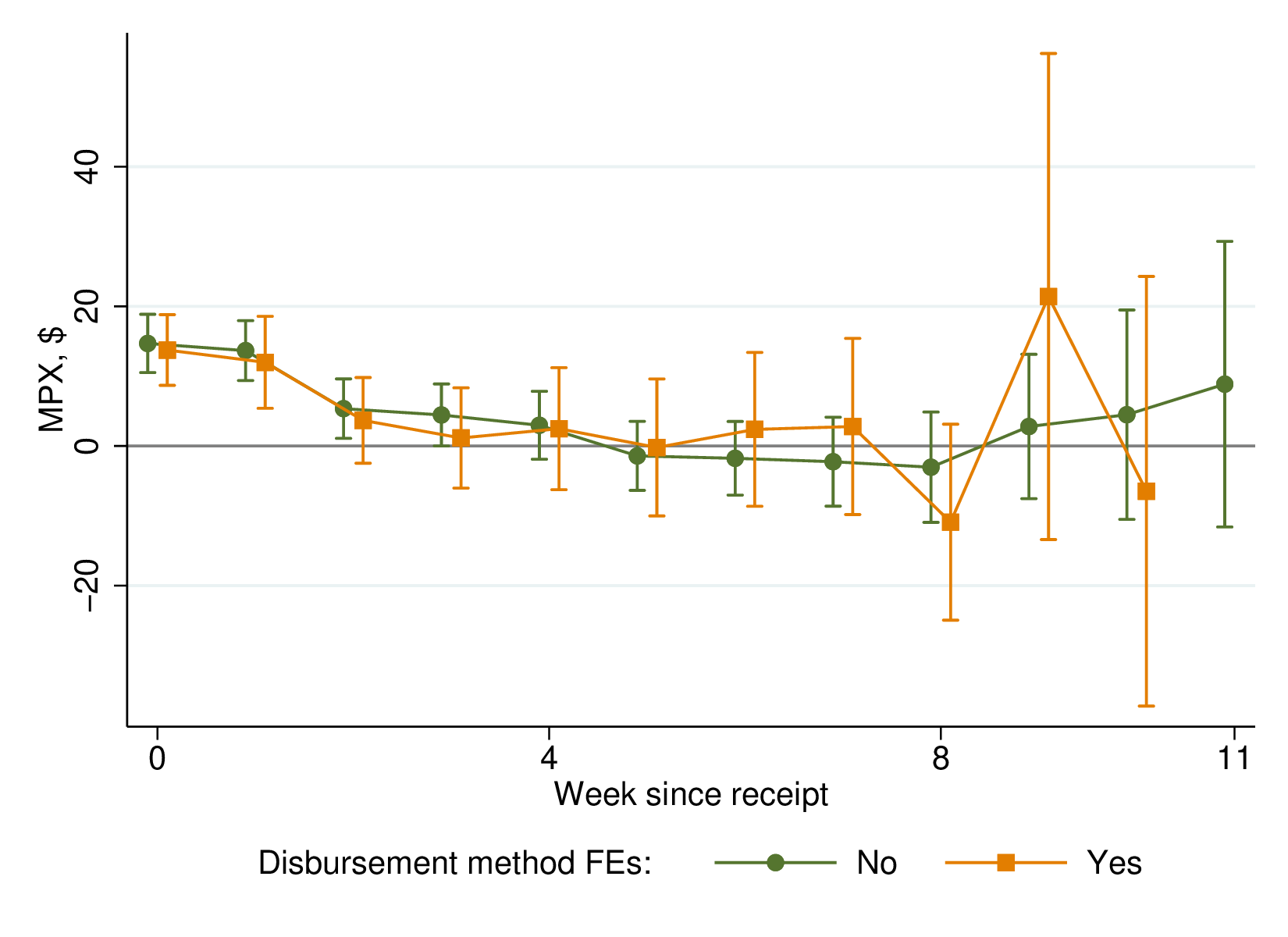
Notes: Panels A–C plot MPX coefficients and 95% confidence bands using the same specifications as in Table 2. Coefficients on the leads of treatment are not shown. The last horizon in Panel B ($h=35$ weeks) and Panel C ($h=12$ weeks without disbursement methods FEs or $h=11$ with FEs) are suppressed because of the very large standard errors, due to a limited sample size. Standard errors are clustered by household.

In Figure 4, we use the same specifications as in Table 2 but we report the full set of dynamic estimates for the treatment effects. Panel A reports the estimates from the binned specification. With disbursement method FEs, the point estimates are large and positive for all nine months following the receipt of the tax rebate. Thus, due to the extrapolation resulting from binning, this specification could be mistakenly interpreted as evidence for a very large and persistent increase in spending. Without these FEs, the estimates tend to hover around zero.

In Panel B, we show estimates with the conventional dynamic specification without binning. Both specifications with and without disbursement method FEs yield point estimates that are almost all negative in the long run. Taken at face value, these estimates could misleadingly suggest that households intertemporally substitute consumption by making purchases at the time of tax rebate that they would have made 20 to 30 weeks later. As in Panel A, these point estimates are noisy but could lend themselves to some economic interpretation.

In contrast, Panel C describes the results from the robust imputation estimator, which does not allow extrapolation in the absence of an explicit control group. This panel shows that, for the horizons for which imputation is possible, there is no evidence of any impact on spending beyond two to four weeks after tax rebate receipt. The patterns are the same both with and without disbursement FEs. These results highlight the practical relevance of the insights from Section 3.4: the imputation estimators avoid extrapolation, thus eliminating seemingly unstable patterns found across conventional specifications.

Figure 5: Underidentification of the Fully-Dynamic Specification

A: Without disbursement method FEs		Panel B: With disbursement method FEs

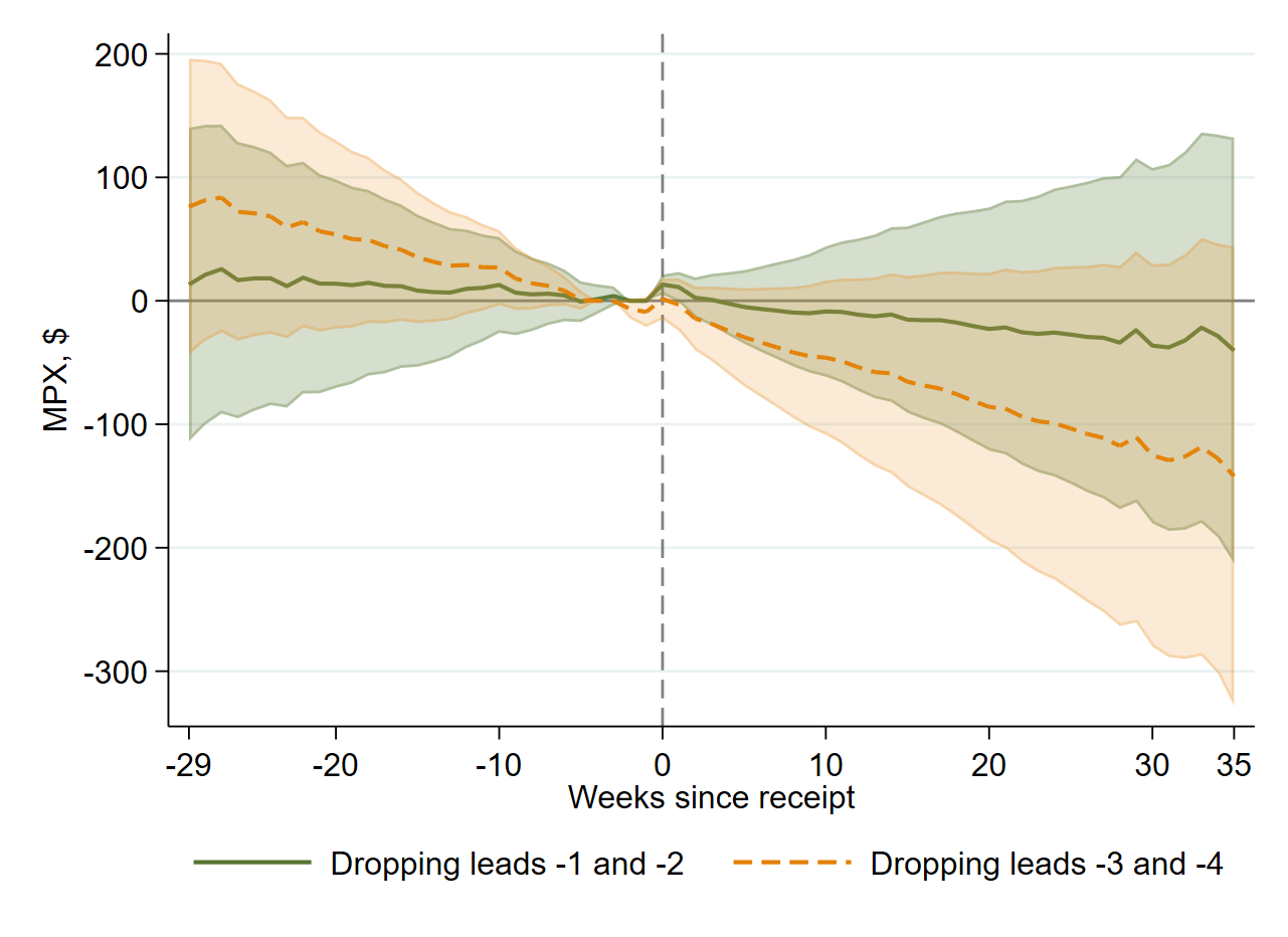
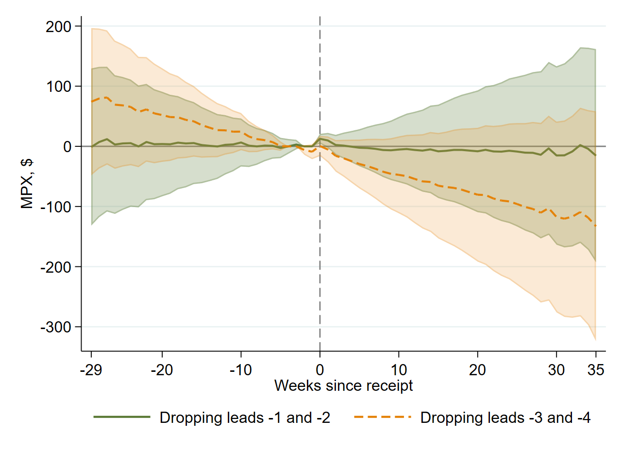
Notes: This figure reports MPX and pre-trend estimates and 95% confidence bands for specification Equation 10 with all leads and lags of the tax receipt included, except for two chosen as indicated. Standard errors are clustered by household.

Finally, in Figure 5 we illustrate the importance of the insights on the underidentification of fully-dynamic specifications from Section 3.2. Unlike earlier specifications, which only included a small number of treatment leads, here we run the specification Equation 10 with a full set of weekly leads and lags around tax rebate receipt. We drop two leads since the set of lead and lag coefficients is only identified up to a linear trend, as discussed in Section 3.2. We find that the fully-dynamic estimates change drastically depending on which two leads are dropped. We illustrate this by comparing the MPXs when dropping leads $-1$ and $-2$ or $-3$ and $-4$. This shows another source of instability in conventional practice, which the imputation estimator directly avoids.

5.2.3 Preferred Robust Estimates and Macroeconomic Implications

We now discuss the implications of our findings for the macroeconomics literature. We proceed in two steps: selecting our preferred MPX estimate from Section 5.2.1 for the Nielsen products and then extrapolating it to broader consumption baskets, following the strategy of BP.

Our preferred estimate for the average cumulative MPX out of the tax rebate for the Nielsen products is $30.5, corresponding to the imputation estimator with disbursement method FEs (Table 2, column 6) in the first month since the rebate. This constitutes 3.4% of the average rebate amount. We choose the specification with disbursement method FEs because the variation in timing is more plausibly exogenous within disbursement methods. We focus on the first (i.e., contemporaneous) month and impose zero effects for the following months based on the evidence from Figures 2 and 4 that the MPXs rapidly decay to zero, while estimation noise increases. Finally, we choose the imputation estimator over conventional specifications for its robustness properties. In contrast to columns 1–2 of Table 2, it avoids the short-term bias due to binning. Moreover, in contrast to column 3–4 it avoids extrapolation of long-run effects (the estimates are similar for the contemporaneous month). Robustness to treatment effect heterogeneity is gained without an efficiency loss in this application: the standard errors are similar across columns of Table 2.

To obtain MPX estimates covering the full consumption basket, BP propose to rescale the estimates obtained with the Nielsen data. This scaling is done in three different ways: (i) by the ratio of spending per capita in the National Income and Product Account (NIPA) and Nielsen data; (ii) by the ratio of the self-reported change in spending on all goods after the rebate relative to that on Nielsen goods alone; (iii) by a factor based on the relative shares of spending and relative responsiveness to the rebate across subcategories of goods as measured in Consumer Expenditure Survey (CE). Using these three approaches and BP’s preferred MPX estimate (reproduced in our Table 2, col. 1), they estimate that the tax rebate raised the annualized expenditure growth rate by 1.3–1.9 percentage points (p.p.) in 2008Q2 and by 0.6–0.9 p.p. in 2008Q3, depending on the choice of rescaling.

Applying the same scaling methods to our preferred MPX estimate for the contemporaneous month and assuming zero response in the following months paints a very different picture, with an increase in annualized expenditure growth of only 0.8–1.1p.p. in 2008Q2 and 0.15–0.22p.p. in 2008Q3. Our estimate implies a 40% smaller response of consumption expenditures in 2008Q2, and 75% smaller in 2008Q3. Correspondingly, while BP conclude that the propensity to spend at the individual level from a tax rebate over three months since the rebate is between 51 and 75 percent, our preferred estimates are half as large, between 25 and 37 percent.

In Table 3, we summarize the MPX estimates for the first quarter after tax rebate obtained with BP’s and our preferred specification. The first row reports the observed marginal propensity to spend on products included in the Nielsen sample during that quarter, as a fraction of the average rebate amount. The next rows rescale these estimates to extrapolate the marginal propensity to spend to broader samples, i.e. the full consumption basket (second row) and nondurables (third row). For the full consumption basket, we implement the three scaling procedures from BP and report the lower and upper bounds; for nondurables we leverage the scaling method of [29]. The fourth row reports the model-consistent, or “notional,” marginal propensity to consume (MPC) that can be used as a target for macroeconomic models, also following the methodology of [29]. The estimates based on BP in column 1 are closely in line with the literature: typical estimates of the quarterly MPX for all expenditures range from 50-90%, while estimates of the quarterly MPX for nondurable expenditure range from 15-25%. In contrast, the imputation estimator in column 2 of Table 3 delivers estimates that are about half as large in all rows. These smaller MPC estimates imply a lower effectiveness of fiscal stimulus.

Table 3: First-quarter MPX and MPC Estimates for Calibration of Macroeconomic Models

Statistic	Replication of	Imputation Estimator
	[7]
	(1)	(2)
Nielsen MPX	6.7%	3.4%
Total MPX	50.8% to 74.8%	24.8% to 36.6%
Nondurable MPX	14.1% to 20.8%	6.9% to 10.2%
Notional MPC	15.9% to 23.4%	7.8% to 11.4%

Notes: This table reports the first-quarter MPX and MPC using the preferred binned specification of [7] and our preferred specification based on the imputation estimator. The first row reports the marginal propensity to spend on products included in the Nielsen sample, as a fraction of the average rebate amount. The second row rescales these estimates to extrapolate them to the marginal propensity to spend on all goods using the three rescaling methods from [7]. The ranges correspond to the lowest and highest values among the three rescaling methods. To obtain the estimate for the nondurables MPX in the third row, we use the scaling factor of [29], who show that the total MPX is equal to 3.6 times the nondurables MPX. The fourth row also follows the methodology of [29] and reports the model-consistent (“notional”) MPC that can be used as a target for macroeconomic models, equal to the total MPX divided by 3.2.

Thus, our new estimates for the impact of the 2008 fiscal stimulus on the U.S. economy yield two lessons for the calibration of macroeconomic models: (1) that the targeted MPC should be significantly smaller — about half as large — and (2) that it is best to calibrate the model using weekly-level estimates of the MPC, as we report in Figure 2, rather than monthly or, especially, quarterly MPC estimates, which are much noisier. Indeed, models should reflect that most of the spending response occurs in the very short run, in the first two to four weeks after tax rebate receipt.

5.3 Efficiency Gains Relative to Alternative Robust Estimators

Finally, we compare the efficiency of the imputation estimator to the alternative robust estimators of [52] and [60], abbreviated dCDH and SA. We document the in-sample efficiency gains in Figure 6 by showing the point estimates and confidence intervals for weekly average MPXs based on the imputation estimator and the two alternatives in Panel A. We use the specification without disbursement method FEs. The point estimates are very similar for dCDH and the imputation estimator, but they differ from those of SA, because this estimator uses a much smaller control group (only the households who received the rebate in the latest possible week) and is therefore much noisier.

Panel B zooms in on the efficiency comparison by reporting the lengths of the confidence intervals for SA and dCDH relative to that of the imputation estimator. The differences are large: the confidence interval from dCDH is about 50% longer for all periods, and 2–3.5 times longer for SA.

In Section A.11 we confirm these efficiency gains, obtained from a single sample, in a Monte Carlo study based on the BP data, for several data-generating processes. We find that the imputation estimator has sizable efficiency advantages over alternative robust estimators not only with spherical errors but also in presence of heteroskedasticity, serial correlation, or both. Moreover, these gains do not come at a cost of systematically higher sensitivity to parallel trend violations. We also confirm that our analytical standard errors have correct coverage.

Figure 6: Alternative Robust MPX Estimates and In-Sample Efficiency

A: Point Estimates		B: Confidence Interval Lengths,
and Confidence Intervals		Relative to the Imputation Estimator

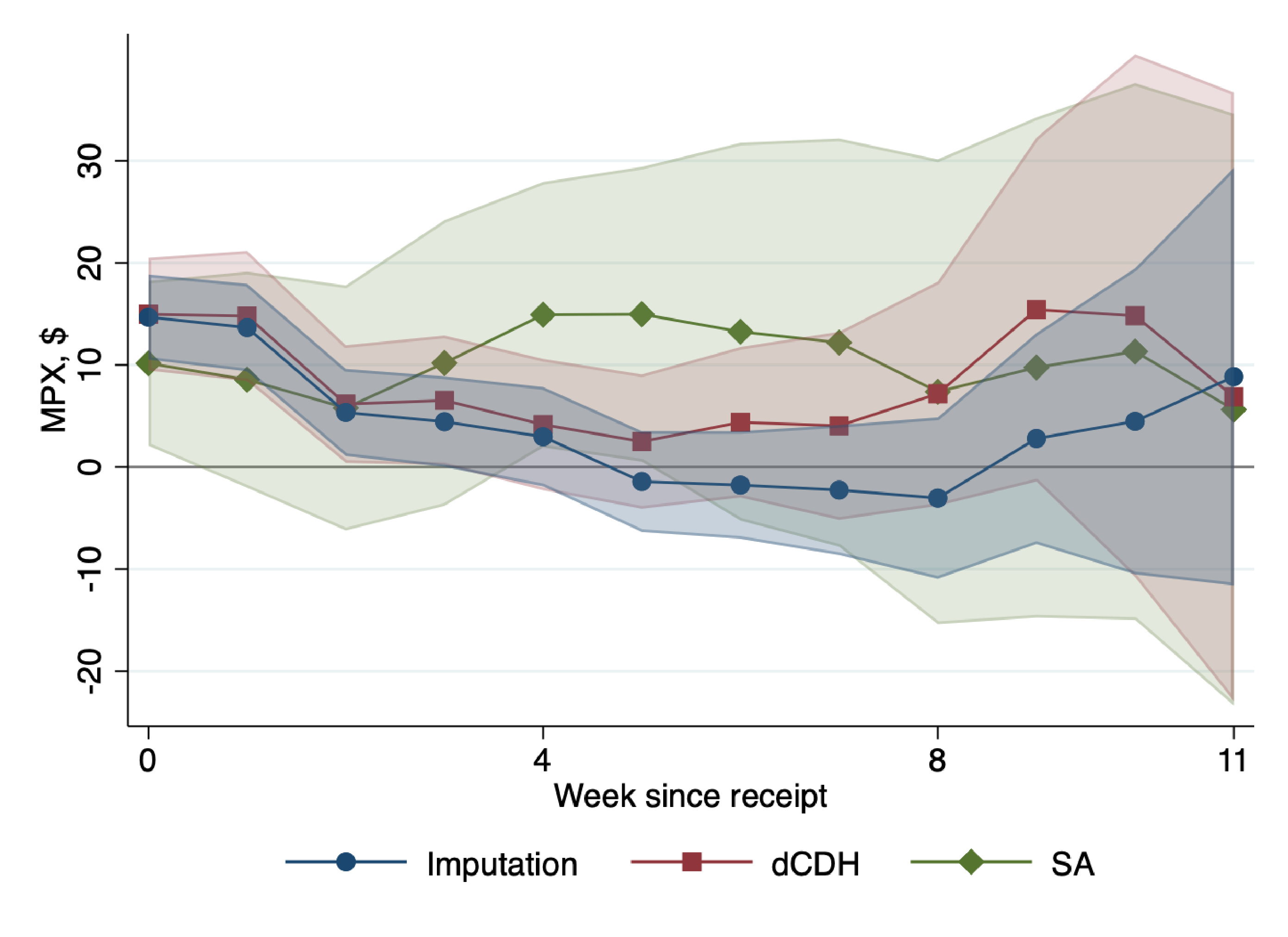
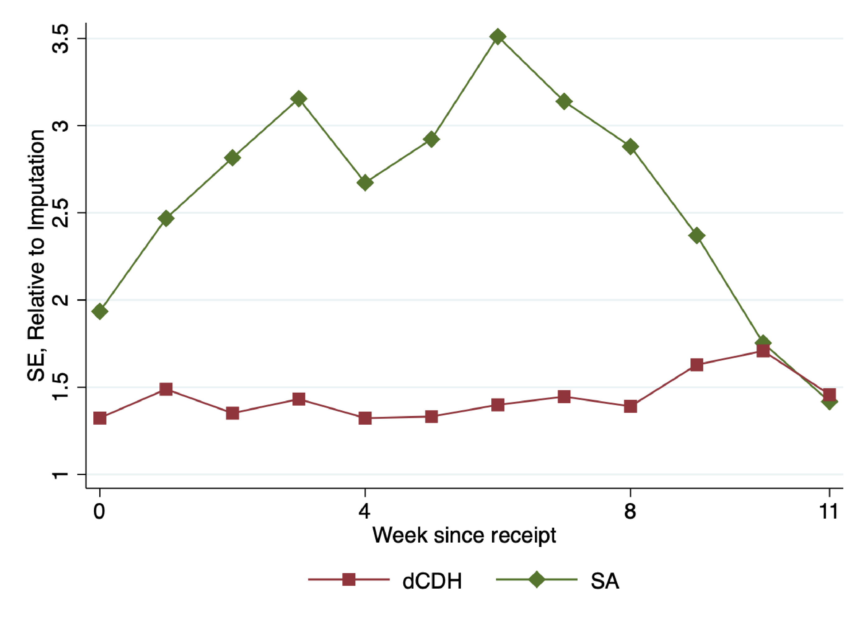
Notes: Panel A shows the estimates and 95% confidence bands for the average MPXs by week since rebate using three robust estimators: the imputation estimator, [52] (dCDH) and [60] (SA). The specifications do not include disbursement method fixed effects. Panel B reports the ratios of the lengths of confidence intervals for dCDH and SA relative to the imputation estimator. Standard errors are clustered by household.

6 Conclusion

In this paper, we provided a unified framework that formalizes an explicit set of goals and assumptions underlying event study designs, reveals and explains challenges with conventional practice, and yields an efficient estimator. In a benchmark case where treatment-effect heterogeneity remains unrestricted, this robust and efficient estimator takes a particularly simple “imputation” form that estimates fixed effects among the untreated observations only, imputes untreated outcomes for treated observations, and then forms treatment-effect estimates as weighted averages over the differences between actual and imputed outcomes. We developed results for asymptotic inference and testing and compared our approach to other estimators. We also highlighted the importance of separating testing of identification assumptions from estimation, which increases estimation efficiency and helps address inference biases due to pre-testing. We demonstrated the practical relevance of these insights in an empirical application documenting that the notional marginal propensity to consume is between 8 and 11 percent in the first quarter, about half as large as benchmark estimates.

Data Availability Statement

The data underlying this article are publicly available on Zenodo, at doi.org/10.5281/zenodo.10037585.

Online Appendix to “Revisiting Event Study Designs: Robust and Efficient Estimation”

Kirill Borusyak, Xavier Jaravel, and Jann Spiess, September 2023

Appendix A Details and Additional Results

A.1 Stochastic Regressors, Exogeneity, and Efficiency

In the main article, we assume that event times, which periods are observed for each unit, and the covariates are non-stochastic. In this section, we show how the generalized fixed-effect model in Section 2 can be obtained from a model where unit-level information is stochastic. This connection allows us to (1) express assumptions about the exogeneity of covariates in a more natural way and (2) expand our efficiency statements beyond the fixed-regressor case. This discussion complements the fixed-regressor approach in the main article, which we choose because it allows for a direct connection to the Gauss–Markov theorem and its efficiency implications.

We now denote by $(Y_{i},Y_{i}(0),A_{i},A_{i}(0),X_{i},X_{i}(0),E_{i},\Omega_{i},\lambda_{i})_{i=1}^{I}$ the relevant variables for a set of $I$ units that are independently distributed across $i$, and where each component of $Y_{i},Y_{i}(0),A_{i},A_{i}(0),\allowbreak X_{i},X_{i}(0)$ collects information for unit $i$ across all time periods, $X_{it}(0)$ and $A_{i}(0)$ are the potential values of covariates in the absence of treatment, and $\Omega_{i}$ collects all periods $t$ for which the outcomes for unit $i$ is observed. We write $\mathcal{I}_{i}=\left(A_{i}(0),X_{i}(0),E_{i},\Omega_{i},\lambda_{i}\right)$ for baseline information about unit $i$, and consider treatment effects $\tau_{it}(\mathcal{I}_{i})=\mathbb{E}\left[Y_{it}-Y_{it}(0)\mid\mathcal{I}_{i}\right]$ for all $t\geq E_{i}$. We now express assumptions on the distribution of the units that allow us to perform causal inference on treatment effects $\tau_{it}(\mathcal{I}_{i})$ based on observations $((Y_{it},A_{it},X_{it})_{t\in\Omega_{i}},E_{i})_{i=1}^{I}$, which expresses that only realized covariates and outcomes for times $t\in\Omega_{i}$ are observed. These assumptions are:

1. The generalized fixed-effects model holds for potential outcomes with strictly exogenous baseline information: $Y_{it}(0)=A_{it}^{\prime}(0)\lambda_{i}+X_{it}^{\prime}(0)\delta+\varepsilon_{it}$ and $\mathbb{E}\left[\varepsilon_{it}\mid\mathcal{I}_{i}\right]=0$ for all $i$ and $t\in\Omega_{i}$;

2. No anticipation: $Y_{it}=Y_{it}(0)$ for all $i$ and $t\in\Omega_{i}$ with $t<E_{i}$;

3. Covariates are causally unaffected by treatment: $A_{it}{=}A_{it}(0)$ and $X_{it}{=}X_{it}(0)$ for all $i$, $t\in\Omega_{i}$.

Here, the strict exogeneity assumption in 1. implies that the relationship of $Y_{it}(0)$ to the control covariates $X_{is}$ for $s\neq t$ and the treatment time $E_{i}$ is fully captured by concurrent covariates $X_{it}$ and the random effect $\lambda_{i}$. The fixed-regressor model is then obtained by conditioning on $\mathcal{I}=(\mathcal{I}_{i})_{i=1}^{I}$, and fulfills Assumptions 1^′, 2 and 5 (provided that the outcomes in the population distribution have bounded second moments).

This formulation also allows us to extend the efficiency results from Section 4 to the case of stochastic regressors. If we consider estimands $\tau_{w}(\mathcal{I})=\sum_{it\in\Omega}w_{it}(\mathcal{I})\>\tau_{it}(\mathcal{I}_{i})$ with weights that are $\mathcal{I}$-measurable and estimators $\hat{\tau}$ that are, conditional on baseline information $\mathcal{I}$, linear in outcomes $Y_{it}$ and unbiased for $\tau_{w}(\mathcal{I})$, then the efficiency results in our fixed-regressor setting still apply since $\mathrm{Var}\left[\hat{\tau}\right]=\mathrm{Var}\left[\mathbb{E}\left[\hat{\tau}\mid\mathcal{I}\right]\right]+\mathbb{E}\left[\mathrm{Var}\left[\hat{\tau}\mid\mathcal{I}\right]\right]$ by the law of total variance, where the first part is pinned down by unbiasedness, and the second part is minimized by an estimator $\hat{\tau}$ that is efficient conditional on baseline information. The conditionally unbiased efficient estimator is therefore the imputation estimator we describe in Section 4. To achieve lower variance than the imputation estimator one would have to forgo unbiasedness conditional on the baseline information $\mathcal{I}$.

A.2 Sampling-Based Parallel Trend Assumptions

In this section, we show that the simple TWFE model in Assumption 1 can be obtained from parallel-trend assumptions formulated in terms of group-wise averages in a population model with randomly sampled units. Our model in Section 2 is therefore more general; it captures common sampling and parallel-trend assumptions, while it allows for more flexible modeling of heterogeneity and may be preferable when the panel is incomplete.

To relate our approach to random sampling with parallel trends, assume now that for a given number $T$ of periods we observe a complete panel of $I$ units with outcomes $Y_{i}=(Y_{i1},\ldots,Y_{iT})$ and treatment time $E_{i}$. We write $Y_{i}(0)=(Y_{i1}(0),\ldots,Y_{iT}(0))$ for the corresponding vector of potential outcomes if the unit was never to be treated. We assume that $(Y_{i,},Y_{i}(0),E_{i})$ are iid across units. We can then impose assumptions on the distribution of $(Y_{i,},Y_{i}(0),E_{i})$:

1. Parallel trends: $\mathbb{E}\left[Y_{i,t+1}(0)-Y_{it}(0)\mid E_{i}\right]$ does not vary with $E_{i}$;

2. No anticipation: $Y_{it}=Y_{it}(0)$ for $t<E_{i}$, a.s.

This formulation is similar to those in e.g. [51, 60, 50], although details vary about the cohorts and periods for which parallel trends are assumed. In this model, we can define unit fixed effects $\alpha_{i}=\mathbb{E}\left[Y_{i1}(0)\mid E_{i}\right]$, period fixed effects $\beta_{t}=\mathbb{E}\left[Y_{it}(0)-Y_{i1}(0)\right]$, and treatment effects $\tau_{it}=\mathbb{E}\left[Y_{it}-Y_{it}(0)\mid E_{i}\right]$, where unit FEs and treatment effects do not vary within cohorts. We then obtain the fixed-regressor model in Section 2 by conditioning on event timing $\left\{E_{i}\right\}_{i}$. Thus, iid sampling, a parallel-trend assumption defined on the cohort level, and a complete panel jointly imply our assumptions in Section 2.

Relative to a sampling-based approach, we see three main advantages of our more general conditional fixed-effects model. First, considering units individually allows us to estimate their treatment effects separately, which permits the estimation of weighted treatment effect sums that put non-constant weights on units with the same relative event time (e.g. when estimating the gap between average treatment effects for men and women two periods since the treatment onset). Second, we can more naturally capture settings in which the convenience assumption of sampling from a population is unrealistic, such as when we observe all US states. Third, our unit fixed-effects model can handle missing observations even when the composition of units changes over time, while cohort-based parallel trend assumptions (e.g. that $\mathbb{E}\left[Y_{i,t+1}(0)-Y_{it}(0)\mid E_{i}\right]$ does not vary with $E_{i}$) may be unattractive; similarly, estimation with cohort, rather than individual, fixed effects can lead to biases with incomplete panels.

A.3 The Challenges Persist when Trimming around Event Times

In this section, we show that the challenges described in Section 3 apply even if the sample is “trimmed” to a fixed window around the event time. By trimming, we mean the relatively common practice (sometimes called “balancing”) of dropping observations more than $a$ periods before or $b$ periods after the event, for some $a>0$ and $b\geq 0$ (e.g. [59], [49]).

One may think that the estimands from static and dynamic conventional specifications may be close to their desirable targets in trimmed samples because by construction the composition of units is unchanged across horizons. However, we show that, with staggered adoption, the weights implied by TWFE regressions can remain complex and highly skewed. Intuitively, this follows because trimmed panels are necessarily unbalanced in terms of units and periods; for instance, the composition of units varies across periods by construction.

To illustrate how the limitations of conventional specifications persist with trimming, and can be made worse, we present a numerical example. In the example, negative weighting in the static TWFE regression is even more severe after trimming. Similarly, weights implied by the dynamic specification with trimming show an even larger skew than without trimming. Finally, trimming can exacerbate the issue of spurious identification of long-run effects. Since trimming also generally reduces the sample size and thus estimation efficiency, it appears difficult to justify. Our numerical example considers five equal-sized cohorts treated in periods $E_{i}=5,\dots,9$ and observed in periods $t=1,\dots,12$, with Assumptions 1 and 2 satisfied in the complete panel. We suppose the researcher decides to trim the sample, keeping four untreated ($K_{it}=-4,\dots,-1$) and four treated ($K_{it}=0,\dots,3$) periods for each unit.

We show that the short-term bias and negative weighting of the static regression persist with trimming. Using the Frisch–Waugh–Lowell theorem, we compute that cumulative weights that the static specification puts on horizons $0,\dots,3$ are 0.875, 0.425, 0.025, and $\text{\textendash}0.325$, respectively (with the penultimate weight combining positive and negative weights on different cohorts). There is more negative weighting with trimming than in the complete panel: the total of all negative weights is $-0.367$ with trimming, compared to $-0.316$ without.

The challenges pertaining to dynamic specifications persist, too. We consider the semi-dynamic specification which includes all lags and no leads of the event, with or without trimming. In our example, we find that the estimands $\tau_{0},\dots,\tau_{3}$ are less homogeneous in trimmed samples in terms of the composition of cohorts underlying them. Figure A1 reports the weights that $\tau_{h}$ places on the observations $h$ periods after treatment across various cohorts, for $h=0,\dots,3$. Panel A, which corresponds to the trimmed sample, shows that all estimands place higher weights on earlier-treated cohorts, but much more so for larger $h$. This is in contrast to the complete panel (Panel B), where the differences both across cohorts and across $h$ are much smaller.

Spurious identification of long-run effects can also be reinforced by trimming, as observations for late-treated units in early periods are dropped. In our example, there are no admissible DiD comparisons for any unit observed three periods after treatment in the trimmed sample, making $\tau_{3}$ identified through extrapolation of treatment effects only. In contrast, admissible comparisons are available in the complete panel: the cohort treated at $E_{i}=5$ and observed at $t=8$ can be compared to that treated at $E_{i}=9$ and to any period $t=1,\dots,4$ when both cohorts are not yet treated.

A.4 Sufficient Conditions for Identification

In this section, we provide sufficient conditions for the identification of $\tau_{w}$. For brevity of notation, we write $A_{it}^{\prime}\lambda_{i}+X_{it}^{\prime}\delta\equiv Z_{it}^{\prime}\pi$, where all parameters $\lambda_{i}$ and $\delta$ are collected into a single column vector $\pi$, with the corresponding covariates collected in $Z_{it}$. We further let $Z$ be the matrix with $N$ rows $Z_{it}^{\prime}$, and $Z_{1}$ and $Z_{0}$ its restrictions to observations $\Omega_{1}$ and $\Omega_{0}$, respectively. Under Assumptions 1^′ and 2, we can therefore write $Y_{it}=Z_{it}^{\prime}\pi+D_{it}\tau_{it}+\varepsilon_{it}$.

Proposition A1 (Sufficient high- and low-level conditions for identification).

Under Assumptions 1^′ and 2 and null Assumption 3^′:

1. In the general case $Y_{it}=Z_{it}^{\prime}\pi_{it}+D_{it}\tau_{it}+\varepsilon_{it}$, write $Z_{1}^{*}=(Z_{it}^{\prime})_{it\in\Omega_{1},w_{it}\neq 0}$ for the matrix with rows $Z_{it}^{\prime}$ corresponding to treated observations with non-zero weights. Then $\tau_{w}$ is identified if $\text{rank}(Z_{0})=\text{rank}\left(\begin{pmatrix}Z_{1}^{*}\\ Z_{0}\end{pmatrix}\right)$.

2. In the specific case $Y_{it}=A_{t}^{\prime}\lambda_{i}+\beta_{t}+D_{it}\tau_{it}+\varepsilon_{it}$ with simple period FEs and unit-specific exposures $\lambda_{i}$ to factors $A_{t}$ that only vary by period (such as unit FEs or unit-specific trends), the following two assumptions are sufficient to ensure identification of $\tau_{w}$:

   1. For every unit $i$ with $\sum_{t;it\in\Omega_{1}}\left|w_{it}\right|>0$, we have that $(A_{t}^{\prime})_{t;it\in\Omega_{0}}$ is of full column rank. (In the TWFE case $A_{t}=1$ this means that for every such unit there is at least one untreated observation. Adding unit-specific trends, two are required.)

   2. There is at least one unit for which untreated outcomes are observed for all time periods up to $T(w)=\max_{t}\left\{\exists i:w_{it}\neq 0\right\}$.

Here, by identification we mean that the parameter is recoverable from the distributions of all outcomes $Y_{it}$. Under these assumptions, two stronger implications are true: first, knowledge of the expectations $\mathbb{E}\left[Y_{it}\right]$ (rather than the full distributions of $Y_{it}$) is sufficient to recover $\tau_{w}$; and second, an unbiased estimator of $\tau_{w}$ exists. Additional conditions, like those we impose in Section 4, are required for such an unbiased estimators to also be consistent (cf. [53] for a discussion of identification and consistency in those separate steps). While Proposition A1 applies in the case of unrestricted treatment-effect heterogeneity, it extends directly to non-trivial Assumption 3^′ since adding structure on the treatment effects only makes identification easier.

A.5 Efficient Estimation beyond Spherical Errors

In this section, we consider an extension of our efficient estimator to the case of non-spherical errors, connecting to the idea of feasible GLS estimation from [62]. The estimator we propose is robust to unrestricted treatment effect heterogeneity, and is efficient if variance–covariance matrices of error terms can be estimated consistently. We illustrate these points in our general model $Y_{it}=Z_{it}^{\prime}\pi+D_{it}\tau_{it}+\varepsilon_{it}$ with unrestricted treatment-effect heterogeneity. We assume observations are independent across units $i$, but unit-level error vectors $\varepsilon_{i}=(\varepsilon_{it})_{t;it\in\Omega}$ can have non-trivial (and unit-specific) variance–covariance matrices $\Sigma_{i}=\textnormal{Var}(\varepsilon_{i})$, which we assume are non-singular. We consider the class of linear estimators $\hat{\tau}_{w}=\sum_{it\in\Omega}v_{it}Y_{it}$ that are unbiased for $\tau_{w}=\sum_{it\in\Omega_{1}}w_{it}\tau_{it}$ under unrestricted treatment-effect heterogeneity, which implies that (and indeed is equivalent to) $v_{it}=w_{it}$ for all $it\in\Omega_{1}$ and $\sum_{it\in\Omega}Z_{it}v_{it}=0$.

We start by expressing the problem of finding the “oracle” efficient unbiased estimator under non-spherical errors. The variance of the linear estimator $\hat{\tau}_{w}=\sum_{it\in\Omega}v_{it}Y_{it}$ is $\mathrm{Var}\left[\hat{\tau}_{w}\right]=\sum_{i}v_{i}^{\prime}\Sigma_{i}v_{i}$ (where we write $v_{i}=(v_{it})_{t;it\in\Omega}$). The efficient oracle estimator is the GLS estimator that minimizes this variance subject to the unbiasedness constraint $\mathbb{E}\left[\hat{\tau}_{w}\right]=\tau_{w}$. Writing $\Sigma_{i}^{1}=\mathrm{Var}\left[\varepsilon_{i}^{0}\right]$ and $\Sigma_{i}^{01}=\mathrm{Cov}\left[\varepsilon_{i}^{0},\varepsilon_{i}^{1}\right]$ for the components of $\Sigma_{i}$ corresponding to the variance of $\varepsilon_{i}^{0}=(\varepsilon_{it})_{t;it\in\Omega_{0}}$ and its covariance with $\varepsilon_{i}^{1}=(\varepsilon_{it})_{t;it\in\Omega_{1}}$, this optimal unbiased estimator has weights $v=(v^{1},v^{0})$ with $v^{1}=w_{1}$ and $v^{0}$ that solve

$$\min_{v^{0}} \sum_{i}v_{i}^{0\prime}\Sigma_{i}^{0}v_{i}^{0}+2v_{i}^{0\prime}\Sigma_{i}^{01}w_{i} w_{1}^{\prime}Z_{1}+v^{0\prime}Z_{0}=0$$ s.t. (11)

If we know the variances $\Sigma_{i}$, then we can find the efficient estimator by solving this straightforward quadratic minimization problem subject to linear constraints. We note that the imputation step, i.e. the solution for $v^{0}$, now depends on the estimand via $w_{it}$, in contrast to the case of spherical errors, which implies $\Sigma_{i}^{01}=\mathbb{O}$.

If we do not have ex-ante knowledge about the variances, then the efficient GLS estimator is not generally feasible since $\Sigma_{i}$ may vary across $i$ with non-iid data. At the same time, we may still be able to obtain a feasible estimator that is asymptotically efficient (in the sense that its asymptotic variance converges to the minimal asymptotic variance among unbiased linear estimators) given a simpler auxiliary model of the variances. Assume that $\Sigma_{i}=\bar{\Sigma}_{i}(\mu)$ with some low-dimensional parameter $\mu$. If required for estimating the variance model consistently, we may further assume that treatment effects themselves follow a model $\tau_{it}=\bar{\tau}_{it}(\mu)$ (where the sets of parameters may or may not overlap). We then consider the following procedure: First, estimate $\mu$ by some $\hat{\mu}$. Then, plug in $\hat{\mu}$ to obtain estimates of the variance matrices $\Sigma_{i}$, the resulting plug-in estimate of $v$ from Equation 11, and the plug-in imputation estimator of $\tau_{w}$.

Consistency and unbiasedness of this estimator do not rely on correctness of the auxiliary model of either treatment effects or variances. Under regularity conditions similar to those in Propositions 8 and A6, and when variance estimates are consistent, we obtain an efficient and robust estimator in the following sense. First, if the model is correct, then the estimator is asymptotically efficient. Second, even if the model is not correct, the estimator is still consistent and asymptotically unbiased for $\tau_{w}$ under unrestricted treatment-effect heterogeneity. We label it the imputation GLS estimator.

We give two examples. First, one can show that our construction yields as a special case the feasible GLS estimator proposed in [62], which we obtain in the case with two-way FEs, no other covariates, and a complete panel, with an auxiliary model $\Sigma_{i}=\bar{\Sigma}(E_{i})$, $\tau_{it}=\bar{\tau}_{t}(E_{i})$ that allows for arbitrary variation across cohorts, but requires homogeneity within.

Second, one may want to leverage a more restricted model of variances to improve small-sample performance. A model which allows the variances to vary arbitrarily across cohort–periods may have too many parameters to allow for an effective estimation of the variance as soon as $T$ is moderately large, in which case the theoretical efficiency gain may not materialize in smaller samples (similar to the findings of [58] on the practical problems with estimating TWFE models using efficient GMM). In such cases, the approach outlined above allows one to instead assume a variance model with fewer parameters. In particular, one could model the errors as an autoregressive process with homoskedastic innovations (e.g., AR(1)), estimate the autoregression parameters, and achieve an efficiency improvement. Using an AR(1) process is enough to bridge the gap between two benchmarks: spherical errors, as in the main text of our paper, and errors following a random walk, as in [55]. In the latter case, [55] has recently derived the Stepwise Difference-in-Differences estimator as the efficient one and shown that it coincides with the [51] estimator for horizon $h=0$.

A.6 Imputation and Weight Representations for Efficient Unbiased Estimators

In this section, we provide several representations of unbiased estimators, both efficient and not, including for the case when a non-trivial treatment-effect model is imposed.

We first show that even when a non-trivial model $\tau=\Gamma\theta$ is imposed, the imputation result for unbiased estimators from Proposition 6 applies with respect to an adjusted estimand.

Proposition A2 (Imputation representation of unbiased estimators with a non-trivial treatment effect model).

Under Assumptions 1^′ and 2, any linear estimator $\hat{\tau}_{w}$ of $\tau_{w}$ that is unbiased when the model $\tau=\Gamma\theta$ is imposed can be written as a linear estimator of some alternatively weighted estimand $\tau_{v}=\sum_{it\in\Omega_{1}}v_{it}\tau_{it}$ that is unbiased without restrictions on the treatment effects. In particular, the imputation representation in Proposition 6 still applies with $\hat{\tau}_{w}=\sum_{it\in\Omega_{1}}v_{it}\hat{\tau}_{it}$ in the third step. The weights $v_{1}=\left(v_{it}\right)_{it\in\Omega_{1}}$ satisfy $\Gamma^{\prime}w_{1}=\Gamma^{\prime}v_{1}$, such that $\tau_{v}=\tau_{w}$ when the model $\tau=\Gamma\theta$ is correct.

We now provide explicit expressions for the weights implied by the the efficient estimator $\hat{\tau}_{w}^{*}$, both with and without Assumption 3^′.

Proposition A3 (Weight representation of efficient estimator).

The efficient estimator from Theorem 1 can be represented as $\hat{\tau}_{w}^{*}=v^{*\prime}Y$ with the weight vector $v^{\ast}=\left(v_{1}^{\ast\prime},v_{0}^{\ast\prime}\right)^{\prime}$ that satisfies

$$v^{*}=\begin{pmatrix}\mathbb{I}-Z_{1}(Z^{\prime}Z)^{-1}Z_{1}^{\prime}\\ -Z_{0}(Z^{\prime}Z)^{-1}Z_{1}^{\prime}\end{pmatrix}\Gamma(\Gamma^{\prime}(\mathbb{I}-Z_{1}(Z^{\prime}Z)^{-1}Z_{1}^{\prime})\Gamma)^{-1}\Gamma^{\prime}w_{1}$$

and that does not depend on the realization of the $Y_{it}$. In the special case of $\Gamma=\mathbb{I}_{N_{1}}$, $v_{1}^{*}=w_{1}$ and $v_{0}^{*}=-Z_{0}(Z_{0}^{\prime}Z_{0})^{-1}Z_{1}^{\prime}w_{1}$.

With a non-trivial Assumption 3^′, we can characterize these weights by a combination of variance minimization for the treated observations and imputation for the untreated observations.

Proposition A4 (Characterization of weights in terms of imputation and variance minimization).

With a non-trivial model $\tau=\Gamma\theta$ for the treatment effects, the efficient estimator from Theorem 1 can be written as the efficient imputation estimator from Theorem 2 under unrestricted heterogeneity with alternative weights $v_{1}^{*}$ on the treatment effects, which solve the variance-minimization problem

$$\min_{v_{1}}\>v_{1}^{\prime}\Phi^{-1}v_{1}\qquad\text{subject to }\Gamma^{\prime}v_{1}=\Gamma^{\prime}w_{1},$$ (12)

where $\Phi=\mathbb{I}_{N_{1}}-Z_{1}(Z^{\prime}Z)^{-1}Z^{\prime}_{1}$ is the variance of the OLS estimator of $\tau$ in the case of spherical errors with unit variance and unrestricted treatment-effect heterogeneity.

A.7 Low-Level Sufficient Asymptotic Conditions

In this section we develop low-level sufficient conditions for consistency, asymptotic normality, and valid inference that directly restrict the weights $w_{1}$ on treated observations and cohort sizes. We focus on the case of a (possibly incomplete) panel with $I$ units and $T$ time periods with respective FEs and no other covariates. We first state sufficient conditions for consistency in a panel where the number of periods $T$ is allowed to grow slowly.

Assumption A1 (Low-level sufficient conditions for consistency).

Assume that in the first period every unit is observed and not treated, and that

1. $\sum_{i=1}^{I}\left(\sum_{t;D_{it}=1}|w_{it}|\right)^{2}\rightarrow 0$, i.e., the weights on treatment effects fulfill a (clustered) Herfindahl condition;

2. $T\sum_{i=1}^{I}\left(\sum_{t;D_{it}=1}w_{it}\right)^{2}\rightarrow 0$, i.e. the concentration of unit net weights decays fast enough;

3. $T^{2}\sum_{t=2}^{T}\frac{(\sum_{i;D_{it}=1}w_{it})^{2}}{\sum_{i;D_{it}=0}1}\rightarrow 0$, i.e., the sum of squared total weight on observations treated at $t$ relative to the number of untreated observations in $t$ vanishes sufficiently quickly.

The first two conditions express that the weights do not concentrate on too few units. They are similar, but not redundant unless $T$ is fixed; when some weights within a unit are negative and some positive, the weights may cancel out within units, yielding the second condition even when the first one is not fulfilled. The three conditions address different sources of variation of the efficient estimator $\hat{\tau}_{w}^{*}$: the first condition bounds the variation from the treated observations themselves; the second, from estimating unit FEs from the untreated observations; and the third, from estimating period FEs from the untreated observations. Together with the conditions in the main text, Assumption A1 yields consistency.

Proposition A5 (Consistency under low-level sufficient conditions).

Suppose Assumptions 1, 2, 5 and A1 hold and treatment effects are allowed to vary arbitrarily (trivial Assumption 3). Then $\hat{\tau}_{w}^{*}$ from Theorem 1 is consistent for $\tau_{w}$.

Next, we develop sufficient conditions that will imply asymptotic normality and valid inference in the special case of a complete panel with a fixed $T$.

Assumption A2 (Low-level sufficient conditions for asymptotic normality and inference).

The panel is complete, $T$ is fixed, $\left|\tau_{it}\right|,$ $\left|\bar{\tau}_{it}\right|$ and $\mathbb{E}\left[\varepsilon_{it}^{4}\right]$ are uniformly bounded, and

1. There is some constant $C$ such that for all $t$ and $i,j$ with $E_{i}=E_{j}$, $D_{it}=1=D_{jt}$ and $w_{it}\neq 0$, we have $w_{jt}\neq 0$ and $\frac{|w_{it}|}{|w_{jt}|}\leq C$; that is, weights do not vary too much within cohort–periods;

2. $\sum_{i;E_{i}=e}1\rightarrow\infty$ for $e=2,\dots,T,\infty$; that is, the size of all cohorts grows.

If we add the latter conditions, we also achieve asymptotic normality.

Proposition A6 (Asymptotic normality in short panels).

Suppose Assumptions 1, 2, 5, A1 and A2 hold, treatment effects are allowed to vary arbitrarily (trivial Assumption 3), and the variance of $\hat{\tau}_{w}^{*}$ does not vanish too quickly, $\liminf n_{H}\sigma_{w}^{2}>0$. Then $\hat{\tau}_{w}^{*}$ from Theorem 1 fulfills the conditions of Proposition 8, and therefore $\sigma_{w}^{-1}(\hat{\tau}_{w}-\tau_{w})\stackrel{{\scriptstyle d}}{{\rightarrow}}\mathcal{N}(0,1).$

Finally, these conditions are also sufficient for obtaining consistent variance estimates.

Proposition A7 (Consistent variance estimation in short panels).

Consider the estimator $\hat{\sigma}_{w}^{2}$ from Theorem 3, and suppose Assumptions 1, 2, 5, A1 and A2 hold and treatment effects are allowed to vary arbitrarily (trivial Assumption 3). Then $\hat{\tau}_{w}^{*}$ from Theorem 1 fulfills the conditions of Theorem 3 when $\tilde{\tau}_{it}$ are equal to an overall average or to cohort–period averages calculated as in equation Equation 8.

We note that Assumptions A1 and A2 are fulfilled in particular in the common case of fixed $T$, growing cohort sizes, and weights that are bounded in the sense that $\sum_{it\in\Omega_{1}}\left|w_{it}\right|<C$ and are constant within cohort–period cells, $w_{it}=w_{jt}$ for $t\geq E_{i}=E_{j}$.

The above conditions apply to the case of unit and time fixed effects. The weight conditions for consistency (Proposition 7) and asymptotic normality (Proposition 8) in the main text can also be verified for more complicated models, such as when there are unit-specific linear trends in addition to fixed effects. As a concrete example, we consider the case of a complete panel of $T=T_{0}+T_{1}$ periods with a single treated cohort of size $I_{1}$, first treated at time $T_{0}+1$, along with a cohort of size $I_{0}$ of never-treated units. For now, suppose we are interested in the average treatment effect in a specific period $t>T_{0}$ for the treated cohort. With some unreported algebra we can calculate weights underlying the imputation estimator with unit and period fixed effects and unit-specific linear trends:

$$v_{is}^{t}=\left(\mathbf{1}\left[s{=}t\right]-\frac{1{+}12\left(s{-}\frac{T_{0}{+}1}{2}\right)\left(t{-}\frac{T_{0}{+}1}{2}\right)/\left(T_{0}^{2}{-}1\right)}{T_{0}}\mathbf{1}\left[s{\leq}T_{0}\right]\right)\cdot\left(\frac{1}{I_{1}}\mathbf{1}\left[E_{i}{=}T_{0}{+}1\right]-\frac{1}{I_{0}}\mathbf{1}\left[E_{i}{=}\infty\right]\right)$$

One can check that these weights satisfy the bound $\sum_{i=1}^{I}\left(\sum_{s=1}^{T}|v_{is}^{t}|\right)^{2}\leq\left(\frac{6t}{T_{0}}\right)^{2}\left(\frac{1}{I_{0}}+\frac{1}{I_{1}}\right)$. The weights therefore fulfill the Herfindahl condition of Assumption 6 (for which Proposition 7 establishes consistency) provided that $I_{0},I_{1}\rightarrow\infty$ and $\frac{T}{T_{0}\sqrt{\min\{I_{0},I_{1}\}}}\rightarrow 0$. The same condition extends to Proposition 8 (asymptotic normality) and the consistency of the imputation estimator of convex averages of the cohort treatment effects.

A.8 Optimal Choices for Treatment Averages in Variance Estimation

The variance estimator in Theorem 3 is asymptotically conservative, since it includes the variation $\sigma_{\tau}^{2}=\sum_{i}\left(\sum_{t;D_{it}=1}v_{it}(\tau_{it}-\bar{\tau}_{it})\right)^{2}\geq 0$ of the treatment effects around their averages $\bar{\tau}_{it}$. Here, we consider reasonable choices for the $\bar{\tau}_{it}$. As discussed in Section 4.3, a natural conservative choice is to estimate a single average $\bar{\tau}_{it}\equiv\bar{\tau}$. The$\bar{\tau}$ that minimizes $\sigma_{\tau}^{2}(\bar{\tau})=\sum_{i}\left(\sum_{t;D_{it}=1}v_{it}(\tau_{it}-\bar{\tau})\right)^{2}$ is

$$\bar{\tau} =\frac{\sum_{i}\left(\sum_{t;D_{it}=1}v_{it}\right)\left(\sum_{t;D_{it}=1}v_{it}\tau_{it}\right)}{\sum_{i}\left(\sum_{t;D_{it}=1}v_{it}\right)^{2}}.$$ (13)

Indeed, $\sigma_{\tau}^{2}(\bar{\tau})$ is convex in $\bar{\tau}$, and the first-order condition $0=\frac{\partial}{\partial\bar{\tau}}\sigma_{\tau}^{2}(\bar{\tau})$ locates the above solution. A natural estimator is its sample analog.

When multiple group-wise averages are estimated, Equation 8 should be viewed as a heuristic extension of Equation 13. The optimal solution for $\tilde{\tau}_{g}$ is generally more complex, as it may depend on treatment effect estimates and weights outside the group. For concreteness, consider averages $\bar{\tau}_{et}$ that vary by cohort $E_{i}=e$ and period $t$, yielding excess variance $\sigma_{\tau}^{2}=\sum_{i}\left(\sum_{t;D_{it}=1}v_{it}(\tau_{it}-\bar{\tau}_{E_{i}t})\right)^{2}$. Then the first-order conditions $0=\frac{\partial}{\partial\bar{\tau}_{es}}\sum_{i}\left(\sum_{t;D_{it}=1}v_{it}(\tau_{it}-\bar{\tau}_{E_{i}t})\right)^{2}=-2\sum_{i;E_{i}=e}v_{is}\left(\sum_{t;D_{it}=1}v_{it}(\tau_{it}-\bar{\tau}_{et})\right)$ have to be solved for each cohort simultaneously across $t$, provided that the estimator puts non-zero weight on multiple periods within the same cohort. The exception is when only one period for every cohort receives non-zero weight, as when estimating the ATT for a given number of periods since treatment. In that situation the optimal solution $\bar{\tau}_{et}=\frac{\sum_{i;E_{i}=e}v_{it}^{2}\tau_{it}}{\sum_{i;E_{i}=e}v_{it}^{2}}$ coincides with equation Equation 13.

A.9 Leave-Out Conservative Variance Estimation

Here we formalize the leave-out conservative variance estimator for $\tau_{w}$, contrast it to leave-out variance estimators from prior work, and provide a computationally efficient way of obtaining them.

As in equation Equation 8, suppose $\Omega_{1}$ is partitioned into groups of treated observations given by $G_{g}$. Let $v_{ig}=\sum_{t;it\in G_{g}}v_{it}$ and $\hat{T}_{ig}=\left(\sum_{t;it\in G_{g}}v_{it}\hat{\tau}_{it}^{*}\right)/v_{ig}$ (with an arbitrary value if $v_{ig}=0$). Then our non-leave-out variance estimator is based on $\tilde{\tau}_{it}\equiv\tilde{\tau}_{g}=\frac{\sum_{j}v_{jg}^{2}\hat{T}_{jg}}{\sum_{j}v_{jg}^{2}}$for $it\in G_{g}$. The leave-out version is defined as $\tilde{\tau}_{it}^{LO}=\frac{\sum_{j\neq i}v_{jg}^{2}\hat{T}_{jg}}{\sum_{j\neq i}v_{jg}^{2}}$.

Our leave-out strategy differs from leave-out variance estimation procedures of [57] and [56]. Those papers assume that the OLS parameter vector is still identified when dropping individual units. In fact, Lemma 1 in [56] shows that unbiased variance estimation is impossible outside that case. Our results, in contrast, provide conservative inference in models where that condition is violated. Indeed, the imputation estimator of Theorem 2 is a special case of Theorem 1 for the model in which each treated observation gets its own treatment effect parameter $\tau_{it}$. Naturally, $\tau_{it}$ cannot be unbiasedly estimated without unit $i$ in the data, and thus the results from [56] do not apply.

While computing $\tilde{\tau}_{it}^{LO}$ directly may be computationally intensive, a more efficient procedure is available based on a simple rescaling of residuals $\tilde{\varepsilon}_{it}$ in equation Equation 7. For $it\in G_{g}$ consider $\tilde{\varepsilon}_{it}^{LO}=\tilde{\varepsilon}_{it}\cdot\frac{1}{1-\left(v_{ig}^{2}/\sum_{j}v_{jg}^{2}\right)}$. Then replacing $\tilde{\varepsilon}_{it}$ with $\tilde{\varepsilon}_{it}^{LO}$ in equation Equation 7 implements the leave-out adjustment (the proof is based on straightforward algebra and available by request). The leave-out variance estimator based on $\tilde{\varepsilon}_{it}^{LO}$ is available as an option in our did_imputation command.

When all residuals use only out-of-cluster observations for estimating $\delta$, too, the resulting variance estimator is exactly unbiased for an upper bound on the true variance:

Proposition A8.

Assume that $\hat{\tau}_{w}$ is unbiased for $\tau_{w}$ and that the variance of $\hat{\tau}_{w}$ is estimated by $\hat{\sigma}_{w}^{2}=\sum_{i}\left(\sum_{t;it\in\Omega}v_{it}\tilde{\varepsilon}_{it}^{LO}\right)^{2}$ with $\tilde{\varepsilon}_{it}^{LO}=Y_{it}-A_{i}^{\prime}\hat{\lambda}_{i}-X_{it}^{\prime}\hat{\delta}^{-i}-D_{it}\tilde{\tau}_{it}^{-i}$, where $\hat{\delta}^{-i}$ and $\tilde{\tau}_{it}^{-i}$ are estimated based on outcomes $Y_{js}$ with $j\neq i$ only, and $\hat{\delta}^{-i}$ is an unbiased estimator of $\delta$. Then $\mathbb{E}\left[\hat{\sigma}_{w}^{2}\right]\geq\sigma_{w}^{2}$.

A.10 Computationally Efficient Calculation of $v_{it}^{\ast}$ Weights

In this section we provide a computationally efficient algorithm for computing the weights $v_{it}^{\ast}$ corresponding to the Theorem 1 estimator. We first establish a general result about the weights underlying any linear combination of estimates in any regression: that the weights can themselves be represented as a linear combination of the regressors, with certain coefficients. We then characterize a system of equations for those coefficients and modify the iterative procedure for computing OLS estimators with high-dimensional FEs to obtain them.

Proposition A9.

Consider some scalar estimator $\hat{\psi}_{w}=w^{\prime}\hat{\psi}$ obtained from an arbitrary point-identified OLS regression $y_{j}=\psi^{\prime}z_{j}+\varepsilon_{j}$. Like every linear estimator, it can be uniquely represented as $\hat{\psi}_{w}=v^{\prime}y$, with $y$ collecting $y_{j}$ and with implied weights $v=\left(v_{j}\right)_{j}$ that do not depend on the outcome realizations. Then weights $v_{j}$ can be represented as a linear combination of $z_{j}$ in the sample, i.e. $v_{j}=z_{j}^{\prime}\check{\psi}$ for some vector $\check{\psi}$, the same for all $j$.

We now apply this proposition to Theorem 1, with the general model of $Y_{it}(0)=Z_{it}^{\prime}\pi+\varepsilon$. Then $\hat{\tau}_{w}^{\ast}=v^{\ast\prime}Y$, where weights $v^{\ast}$ can be represented as $v_{it}^{\ast}=Z_{it}^{\prime}\check{\pi}+D_{it}\Gamma_{it}^{\prime}\check{\theta}.$ It remains to find the unknown $\check{\pi}$ and $\check{\theta}$ to obtain the $v^{\ast}$ weights. To do so, we use the properties of $\hat{\tau}_{w}^{\ast}$. First, it equals to zero if $Y_{it}$ is linear in $Z_{it}$. Second, letting $\mu=\Gamma^{\prime}w_{1}$, $\hat{\tau}_{w}^{\ast}=\mu_{j}$ if $Y_{it}=\Gamma_{it,j}D_{it}$ for all $it\in\Omega$, as in that case $\hat{\theta}_{j}=1$ and $\hat{\theta}_{-j}=0$. Thus we have a system of equations which determine $\check{\pi}$ and $\check{\theta}$:

$$\sum_{it\in\Omega}Z_{it}\left(Z_{it}^{\prime}\check{\pi}+D_{it}\Gamma_{it}^{\prime}\check{\theta}\right) =0; \sum_{it\in\Omega_{1}}\Gamma_{it}\left(Z_{it}^{\prime}\check{\pi}+D_{it}\Gamma_{it}^{\prime}\check{\theta}\right) =\Gamma^{\prime}w_{1}.$$ (14)

When $Z_{it}$ has a block structure in which some covariates are FEs, solving this system iteratively is most convenient and computationally efficient. For instance, suppose $Z_{it}^{\prime}\pi\equiv\alpha_{i}+X_{it}^{\prime}\delta$ and $\Gamma=\mathbb{I}_{N_{1}}$ (i.e. Assumption 3^′ is trivial). Then Proposition A9 implies $v_{it}^{\ast}=\check{\alpha}_{i}+X_{it}^{\prime}\check{\delta}+D_{it}^{\prime}\check{\theta}_{it}$ for all $it\in\Omega$, and the second part of Equation 14 simplifies to $v_{it}^{\ast}=w_{it}$ for all $it\in\Omega_{1}$. Using this and the structure of $Z_{it}$, we rewrite the first part of Equation 14 as a system

$$\sum_{t,\ it\in\Omega_{0}}\left(\check{\alpha}_{i}+X_{it}^{\prime}\check{\delta}\right) =-\sum_{t,\ it\in\Omega_{1}}w_{it},\quad\text{for all }i;$$ (15)

$$\sum_{it\in\Omega_{0}}X_{it}\left(\check{\alpha}_{i}+X_{it}^{\prime}\check{\delta}\right) =-\sum_{it\in\Omega_{1}}X_{it}w_{it}.$$ (16)

This system suggests an algorithm similar to iterative OLS [[, e.g.]]Guimaraes2010:

1. Given a guess of $\check{\delta}$, set $\check{\alpha}_{i}$ for each unit to satisfy Equation 15;

2. Given $\check{\alpha}_{i}$, set $\check{\delta}$ to satisfy Equation 16;

3. Repeat until convergence.

A.11 Monte-Carlo Simulation

We now quantify the efficiency properties of the imputation estimator in a simulation based on the BP application, both under homoskedastic, serially uncorrelated error terms and without those assumptions. We compare the imputation estimator to the alternative robust estimators of [52] and [60], as well as to conventional dynamic specifications in terms of efficiency and bias. We also verify correct coverage of our inference procedure and check sensitivity of different estimators to anticipation effects.

Setting.

Our baseline simulation uses the sample and treatment timing from the application of Section 5; in line with Section 2, we view them as non-stochastic. Our target estimands are the ATTs $\tau_{h}$ for each horizon $h=0,\dots,11$ (in dollars); while $\tau_{0}$ is an average of the short-run effects on 21,545 units, $\tau_{11}$ corresponds to 1,498 units only.

In order to simulate data, we obtain estimates of treatment effects and residuals from the data. We first apply the imputation estimator to the observed data (without disbursement method FEs) to obtain $\hat{\tau}_{it}$ and, for the untreated observations, residuals $\tilde{\varepsilon}_{it}$, as in Equation 7. We then compute $\tilde{\tau}_{it}$ as the average of $\hat{\tau}_{it}$ within each cohort-period cell (using projection weights) for horizons $h=0,\dots,3$. For $h>3$ we set $\tilde{\tau}_{it}=0$, based on the main draft’s findings that the MPXs decay quickly. We set $\tilde{\varepsilon}_{it}=\hat{\tau}_{it}-\tilde{\tau}_{it}$ for treated observations, attributing the within-cell variation in treatment effects to the residual. In the simulations we use $\tilde{\tau}_{it}$ as the true treatment effects and consider several DGPs for the error terms. In the baseline version, the error terms are spherical with the variance equal to $\sigma_{\tilde{\varepsilon}}^{2}$, the sample variance of $\tilde{\varepsilon}_{it}$.

We compare the efficiency of the imputation estimator to those of the [52] and [60] estimators (denoted dCDH and SA, respectively). Two versions of the [50] estimator are equivalent to dCDH and SA, respectively, in this setting with no additional covariates. Importantly, the estimands are exactly the same for all three robust estimators we consider. We further consider two versions of OLS estimators: semi-dynamic, which includes all lags but no leads of treatment, and fully-dynamic, which further includes all leads except $h=-1$ and $h=-5$. For each estimator, we compute the underlying weights $v_{it}$ and use them to calculate the exact properties of the estimators, such as their finite-sample variance. For inference on the imputation estimator, we use the results from Section 4.3. In the absence of treatment effect heterogeneity within cohort-period cells, inference is asymptotically exact rather than conservative.

Results.

We first compare the imputation estimator to its robust counterparts. Panel 1a of Figure A2 reports the exact standard deviation of each estimator, for each horizon-specific estimand, and Panel 2a shows it relative to the imputation estimator. In line with Theorem 1, the imputation estimator is most efficient among the robust estimators for all horizons, but the simulation is useful in quantifying the magnitude of the efficiency gain. Under homoskedasticity, the standard deviations (SDs) of the dCDH estimator are 35–39% higher than the SD of the imputation estimator, implying that 82–92% more units would be needed to obtain confidence intervals of a similar length if these estimators are used. SDs of the SA estimator, which uses a smaller reference group, are much higher yet: 39–290% higher than with imputation.

In Panels 1b–1d and 2b–2d of Figure A2, we report estimator SDs under deviations from spherical errors, such that the relative efficiency of the imputation estimator is no longer guaranteed by Theorem 1. In Panels 1b and 2b we make the error terms heteroskedastic in a way implied by the data (while still mutually independent): $\varepsilon_{it}\sim\mathcal{N}(0,\sigma_{it}^{2})$ for $\sigma_{it}^{2}=\tilde{\varepsilon}_{it}$. In Panels 1c and 2c we instead suppose that $\varepsilon_{it}$ follow a stationary AR(1) process with $\mathrm{Var}\left[\varepsilon_{it}\right]=\sigma_{\tilde{\varepsilon}}^{2}$ and $\mathrm{Cov}\left[\varepsilon_{it},\varepsilon_{it^{\prime}}\right]=0.5^{\lvert t-t^{\prime}\rvert}$, with $\varepsilon_{it}$ still normally distributed and independent across units. In Panels 1d and 2d we finally learn the patterns of both heteroskedasticity and serial correlation from the data by using wild clustered bootstrap, i.e. setting $\varepsilon_{it}=z_{i}^{\ast}\tilde{\varepsilon}_{it}$ for $z_{i}^{\ast}$ drawn independently across households and taking values $\pm 1$ with equal probabilities. The imputation estimator remains the most efficient of the three, with SDs of dCDH (SA) higher by 32–56% (48–264%) in Panel 2b, 13–38% (43–343%) in Panel 2c, and 34–66% (42–249%) in Panel 2d. The only exception is for $h=0$ with AR(1) errors, where the dCDH estimator has a 2% lower SD.

Panels 1–2 of Figure A2 also compare the imputation estimator to conventional OLS estimators, showing that the robustness to treatment effect heterogeneity associated with the imputation estimator comes at a nearly zero efficiency cost for the shorter horizons, $h=0,1,2$. Across the four DGPs, the SD of the semi-dynamic OLS estimator is at most 13% lower than that of the imputation estimator. Moreover, the SD of fully-dynamic OLS is in most cases higher than that of the imputation estimator, as the former does not fully impose Assumption 2. For longer horizons, the efficiency advantage of the semi-dynamic estimator is larger. These efficiency gains come at a cost of a small bias, reported in Panel 3; the bias is guaranteed to be zero for the imputation estimator. Because of the bias, the advantage of the semi-dynamic estimator shrinks slightly, when measured by the root mean squared error in Panel 4.

In Panel 5 we consider the sensitivity of different estimators to anticipation effects. We add an anticipation effect of $10 to the outcomes of each household in the period right before treatment, $t=E_{i}-1$, and report the exact bias of each estimator due to this. We find the imputation estimator to be uniformly less sensitive than its robust alternatives, although the semi-dynamic OLS specification has an even smaller bias.

Finally, we verify that the inference procedure for the imputation estimator proposed in Section 4.3 performs well. Panel 6 reports its simulated coverage: the fraction of the 1,000 simulations in which a $t$-test does not reject the null of $\tau_{h}$ taking its “true” value at the 5% significance level (as implemented via our Stata command did_imputation), across the four DGPs for the errors. The rejection rate is close to 5% across all horizons and DGPs.

Taken together, these results suggest that the imputation estimator has sizable efficiency advantages over alternative robust estimators, extending to heteroskedasticity and serial correlation of error terms. The analysis further highlights that the efficiency gains do not come at a cost of systematically higher sensitivity to parallel-trend violations. Moreover, our analytical inference tools perform well in finite samples, and the efficiency costs relative to dynamic OLS estimators are low, except for long-run effects. Naturally, these results may be specific to the data-generating processes we considered, and we recommend that researchers perform similar simulations based on their data.

A.12 Equal Sensitivity of Robust Estimators to Linear Pre-Trends

Proposition A10.

Suppose there are no never-treated units. Then all linear estimators $\hat{\tau}_{w}$ of $\tau_{w}$ that are unbiased under Assumptions 1 and 2 with a trivial Assumption 3, and thus robust to arbitrary treatment effect heterogeneity, have the same sensitivity to linear anticipation trends. Specifically, if $Y_{it}=\left(\kappa_{0}+\kappa_{1}K_{it}\right)\cdot\mathbf{1}\left[D_{it}=0\right]$ for some $\kappa_{0},\kappa_{1}\in\mathbb{R}$, then $\mathbb{E}\left[\hat{\tau}_{w}\right]=-\sum_{it\in\Omega_{1}}w_{it}\left(\kappa_{0}+\kappa_{1}K_{it}\right)$.

This result implies that there cannot be a general ranking in the sensitivity of different estimators to anticipation effects. We formalize this intuition by:

Corollary A1.

For an estimator $\hat{\tau}_{w}$ of $\tau_{w}$ that is unbiased under unrestricted treatment effect heterogeneity and $y_{0}\in\mathbb{R}^{\left|\Omega_{0}\right|}$, let $B_{\hat{\tau}_{w}}(y_{0})$ be its bias when $\mathbb{E}\left[Y_{0}\right]=y_{0}$, potentially violating Assumptions 1 and 2. Consider two such linear estimators, $\hat{\tau}_{w}^{A}$ and $\hat{\tau}_{w}^{B}$, and suppose $\hat{\tau}_{w}^{A}$ is more biased for some $y_{0}$, $\lvert B_{\hat{\tau}_{w}^{A}}(y_{0})\rvert>\lvert B_{\hat{\tau}_{w}^{B}}(y_{0})\rvert$. Then there exists $\tilde{y}_{0}\in\mathbb{R}^{\left|\Omega_{0}\right|}$ such that the comparison is reversed, $\lvert B_{\hat{\tau}_{w}^{B}}(\tilde{y}_{0})\rvert>\lvert B_{\hat{\tau}_{w}^{A}}(\tilde{y}_{0})\rvert$.

Appendix B Proofs

In this appendix, we collect proofs for the results in the main text and in the appendix. We first restate our general matrix notation for convenience. Specifically, we stack the vectors $\lambda_{i}$ into a single vector $\lambda=(\lambda_{i})_{i}$. We set $Z_{it}=\begin{pmatrix}(\mathbf{1}\left[i=j\right]A_{jt})_{j}\\ X_{it}\end{pmatrix},\pi=\begin{pmatrix}\lambda\\ \delta\end{pmatrix}$ to summarize the nuisance component of the model. In matrix-vector notation, we write $Y$ for the vector of outcomes, $Z=(A,X)$ for the covariate matrix, $D$ for the matrix of indicators for treated units, $\varepsilon$ for the vector of error terms, and $\Sigma=\mathrm{Var}\left[\varepsilon\right]$ for their variance. We write $Y_{1},Z_{1}=(A_{1},X_{1}),D_{1},\varepsilon_{1}$ for the rows corresponding to treated observations ($it\in\Omega_{1}$); in particular, $D_{1}=\mathbb{I}$. Analogously, we write $Y_{0},Z_{0}=(A_{0},X_{0}),D_{0},\varepsilon_{0}$ for the rows corresponding to untreated observations ($it\in\Omega_{0}$); in particular, $D_{0}=\mathbb{O}$. We write $\tau=(\tau_{it})_{it\in\Omega_{1}}$ for the vector of treatment effects of the treated units, $\theta=(\theta_{m})_{m=1}^{N_{1}-M}$ for the vector of underlying parameters, $\Gamma=(\Gamma_{it,j})_{it\in\Omega_{1},j\in\{1,\ldots,N_{1}-M\}}$ for the matrix linking the two, and $w_{1}=(w_{it})_{it\in\Omega_{1}}$ for the weight vector. Then we can write model and estimand as

$$Y=Z\pi+D\tau+\varepsilon,\qquad\tau=\Gamma\theta,\qquad\tau_{w}=w_{1}^{\prime}\tau,$$

where $\mathbb{E}\left[\varepsilon\right]=\textbf{0}$, $\mathrm{Var}\left[\varepsilon\right]=\Sigma$, and $\Sigma$ has block structure according to units $i$. For unit $i$, we write $A_{i}=(A_{it})_{t},X_{i}=(X_{it})_{t},Y_{i}=(Y_{it})_{t},\varepsilon_{i}=(\varepsilon_{it})_{t},v_{i}=(v_{it})_{t}$ and denote by $\Sigma_{i}=\mathrm{Var}\left[\varepsilon_{i}\right]$ the within-unit variance–covariance matrix of error terms.

B.1 Proofs of Results from Main Text

Proof of Proposition 1.

In the absence of never-treated units and defining $\tau_{-1}=0$, we can write $\sum_{h\neq-1}\tau_{h}\mathbf{1}\left[K_{it}=h\right]=\tau_{K_{it}}.$ Now consider some collection of $\tau_{h}$ (with $\tau_{-1}=0$) and FEs $\tilde{\alpha}_{i}$ and $\tilde{\beta}_{t}$. For any $\kappa\in\mathbb{R}$, let $\tau_{h}^{\star}=\tau_{h}+\kappa\left(h+1\right)$, $\tilde{\alpha}_{i}^{\star}=\tilde{\alpha}_{i}+\kappa\left(E_{i}-1\right)$, and $\tilde{\beta}_{t}^{\star}=\tilde{\beta}_{t}-\kappa t$. Then for any observation $it$, $\tilde{\alpha}_{i}^{\star}+\tilde{\beta}_{t}^{\star}+\tau_{K_{it}}^{\star}=\tilde{\alpha}_{i}+\tilde{\beta}_{t}+\tau_{K_{it}}+\kappa\left(E_{i}-1\right)-\kappa t+\kappa\left(t-E_{i}+1\right)=\tilde{\alpha}_{i}+\tilde{\beta}_{t}+\tau_{K_{it}}$, and equation Equation 2 has exactly the same fit under the original and modified FEs and $\tau_{h}$ coefficients, indicating perfect collinearity. ∎

Proof of Proposition 2.

By the Frisch–Waugh–Lovell theorem, $\tau^{\text{static}}$ can be obtained by a regression of $\mathbb{E}\left[Y_{it}\right]=\alpha_{i}+\beta_{t}+\tau_{it}D_{it}$ on $\tilde{D}_{it}$ (without a constant), where $\tilde{D}_{it}=D_{it}-\check{\alpha}_{i}-\check{\beta}_{t}$ are the residuals from the auxiliary regression of $D_{it}$ on the unit and period FEs. Thus, $\tau^{\text{static}}=\frac{\sum_{it\in\Omega}\tilde{D}_{it}\left(\alpha_{i}+\beta_{t}+\tau_{it}D_{it}\right)}{\sum_{it\in\Omega}\tilde{D}_{it}^{2}}.$ We have $\sum_{it\in\Omega}\tilde{D}_{it}\alpha_{i}=\sum_{i}\alpha_{i}\sum_{t;it\in\Omega}\tilde{D}_{it}=0$ because the residuals in the auxiliary regression are orthogonal to all unit indicators. Analogously, $\sum_{it\in\Omega}\tilde{D}_{it}\beta_{t}=0$. Defining

$$w_{it}^{\text{static}}=\frac{\tilde{D}_{it}}{\sum_{it\in\Omega}\tilde{D}_{it}^{2}},$$ (17)

we have that $\tau^{\text{static}}=\sum_{it\in\Omega}w_{it}^{\text{static}}\tau_{it}D_{it}=\sum_{it\in\Omega_{1}}w_{it}^{\text{static}}\tau_{it}$, as required. Clearly, $w_{it}^{\text{static}}$ do not depend on the outcome realizations. Moreover, these weights add up to one because we have that $\sum_{it\in\Omega_{1}}\tilde{D}_{it}=\sum_{it\in\Omega}\tilde{D}_{it}D_{it}=\sum_{it\in\Omega}\tilde{D}_{it}\left(\tilde{D}_{it}+\check{\alpha}_{i}+\check{\beta}_{t}\right)=\sum_{it\in\Omega}\tilde{D}_{it}^{2}$, where the last equality holds because $\tilde{D}_{it}$ are orthogonal to the unit and period FEs. ∎

Proof of Proposition 3.

We use the characterization of the static TWFE specification weights in equation Equation 17. Given the complete panel, the regression of $D_{it}$ on TWFE produces residuals $\tilde{D}_{it}=D_{it}-\bar{D}_{i\cdot}-\bar{D}_{\cdot t}+\bar{D}_{\cdot\cdot}$, where $\bar{D}_{i\cdot}=\frac{1}{3}\sum_{t=1}^{3}D_{it}$, $\bar{D}_{\cdot t}=\frac{1}{2}\sum_{i=A,B}D_{it}$, and $\bar{D}_{\cdot\cdot}=\frac{1}{6}\sum_{i=A,B}\sum_{t=1}^{3}D_{it}$ [51]. Plugging in $\bar{D}_{A\cdot}=2/3$, $\bar{D}_{B\cdot}=1/3$, $\bar{D}_{\cdot 1}=0$, $\bar{D}_{\cdot 2}=1/2$, $\bar{D}_{\cdot 3}=1$, and $\bar{D}_{\cdot\cdot}=1/2$, and computing $\sum_{it\in\Omega_{1}}\tilde{D}_{it}=1/3$, we have

$$\hat{\tau}^{\text{static}} =\frac{\sum_{it\in\Omega}\tilde{D}_{it}Y_{it}}{\sum_{it\in\Omega_{1}}\tilde{D}_{it}}=\left(Y_{A2}-Y_{B2}\right)-\frac{1}{2}\left(Y_{A1}-Y_{B1}\right)-\frac{1}{2}\left(Y_{A3}-Y_{B3}\right).$$

Similarly, the static estimand equals $\tau^{\text{static}}=\frac{\sum_{it\in\Omega_{1}}\tilde{D}_{it}\tau_{it}}{\sum_{it\in\Omega_{1}}\tilde{D}_{it}}=\tau_{A2}-\frac{1}{2}\left(\tau_{A3}-\tau_{B3}\right).$ ∎

Proof of Proposition 4.

Let $I$ be the total number of units and $I_{\text{ever}}$ be that of ever-treated units (those treated by $t=T$). As in the proofs of Propositions 2 and 3, $w_{it}^{\text{static}}=\tilde{D}_{it}/\sum_{it\in\Omega}\tilde{D}_{it}^{2}$ with

$$\tilde{D}_{it}=D_{it}-\bar{D}_{i\cdot}-\bar{D}_{\cdot t}+\bar{D},$$ (18)

for $\bar{D}_{i\cdot}=\frac{1}{T}\sum_{t=1}^{T}D_{it}=\frac{T-\left(E_{i}-1\right)}{T}$, $\bar{D}_{\cdot t}=\frac{1}{I}\sum_{i=1}^{I}D_{it}=\frac{\sum_{i}\mathbf{1}\left[E_{i}\leq t\right]}{I}$, and $\bar{D}_{\cdot\cdot}=\frac{1}{IT}\sum_{i,t}D_{it}=\frac{I_{\text{ever}}\left(T-\left(E_{\text{first}}-1\right)\right)-N_{0}^{\ast}}{IT}$, where the last expression holds because treated observations are those belonging to ever-treated units in periods since $E_{\text{first}}$, excluding the $N_{0}^{\ast}$ pre-treatment observations.

Since $\bar{D}_{i\cdot}$ monotonically declines in $E_{i}$ and $\bar{D}_{\cdot t}$ increases in $t$, equation Equation 18 implies that the lowest weight on any treated observation corresponds to $E_{i}=E_{\text{first}}$ and $t=T$. Thus, there is no negative weighting if and only if $\tilde{D}_{it}\geq 0$ for such observations. Considering equation Equation 18 for one of those observations and using $\bar{D}_{\cdot T}=\frac{I_{\text{ever}}}{I}$, there is no negative weighting if and only if

$$0 \leq 1-\frac{T-\left(E_{\text{first}}-1\right)}{T}-\frac{I_{\text{ever}}}{I}+\frac{I_{\text{ever}}\left(T-\left(E_{\text{first}}-1\right)\right)-N_{0}^{\ast}}{IT}=\frac{N_{1}^{\ast}-N_{0}^{\ast}}{IT},$$

where the last equality uses the definition of $N_{1}^{\ast}$. This is equivalent to $N_{1}^{\ast}\geq N_{0}^{\ast}$, as required. ∎

Proof of Proposition 5.

For any observation $it$, $K_{it}=t-E_{i}\geq\bar{H}$ implies $t\geq E_{i}+\bar{H}\geq\min_{i}E_{i}+\bar{H}\geq\max_{i}E_{i}$. Thus, all observations considered by the estimand correspond to the periods in which all units are already treated. Consider one such period $t^{\star}$ for which the total weights are non-zero, $\sum_{i\colon K_{it^{\star}}\geq\bar{H}}w_{it}\neq 0$. (It exists because all weights $w_{it}$ are assumed non-negative and are not identically zero.) Then consider a data-generating process in which $\beta_{t^{\star}}$ is replaced with $\beta_{t^{\star}}-\kappa$ for some $\kappa\neq 0$ and $\tau_{it^{\star}}$ is replaced with $\tau_{it^{\star}}+\kappa$ for all $i$. This DGP is observationally equivalent in terms of the observed $Y_{it}$ and continues to satisfy Assumptions 1 and 2. Yet, the estimand differs by any arbitrary $\kappa\sum_{i\colon K_{it^{\star}}\geq\bar{H}}w_{it}\neq 0$, and is therefore not identified. ∎

Proof of Theorem 1.

The result is a consequence of the Gauss–Markov theorem. By itself, the Gauss–Markov theorem establishes the efficiency of the OLS estimator for $\theta$. Here, we extend efficiency of the estimation of $\theta$ to efficiency for the estimation of the weighted sum of treatment effects $\tau_{w}=w_{1}^{\prime}\Gamma\theta$. By construction, $\hat{\tau}_{w}^{*}=w_{1}^{\prime}\Gamma\hat{\theta}^{*}$ for the OLS estimator $\hat{\theta}^{*}$ of $\theta$. For every linear estimator $\hat{\tau}_{w}$ that is unbiased for $\tau_{w}$ for all $\theta$ there is a linear unbiased estimator $\hat{\theta}$ of $\theta$ (with variance $\Sigma_{\hat{\theta}}$) for which $\tilde{\tau}_{w}=w_{1}^{\prime}\Gamma\hat{\theta}$, for example the estimator $\hat{\theta}=\hat{\theta}^{*}+\Gamma^{\prime}w_{1}(w_{1}^{\prime}\Gamma\Gamma^{\prime}w_{1})^{-1}(\hat{\tau}_{w}-w_{1}^{\prime}\Gamma\hat{\theta}^{*})$ (where we assume that $\Gamma^{\prime}w_{1}\neq\textbf{0}$, since the estimand and efficient estimator are otherwise zero). Indeed,

$$w_{1}^{\prime}\Gamma\hat{\theta} =w_{1}^{\prime}\Gamma\hat{\theta}^{*}+w_{1}^{\prime}\Gamma\Gamma^{\prime}w_{1}(w_{1}^{\prime}\Gamma\Gamma^{\prime}w_{1})^{-1}(\hat{\tau}_{w}-w_{1}^{\prime}\Gamma\hat{\theta}^{*})=\hat{\tau}_{w},$$

$$\mathbb{E}\left[\hat{\theta}\right] =\mathbb{E}\left[\hat{\theta}^{*}\right]+\Gamma^{\prime}w_{1}(w_{1}^{\prime}\Gamma\Gamma^{\prime}w_{1})^{-1}\left(\mathbb{E}\left[\hat{\tau}_{w}\right]{-}\mathbb{E}\left[w_{1}^{\prime}\Gamma\hat{\theta}^{*}\right]\right)=\theta+\Gamma^{\prime}w_{1}(w_{1}^{\prime}\Gamma\Gamma^{\prime}w_{1})^{-1}(w_{1}^{\prime}\Gamma\theta{-}w_{1}^{\prime}\Gamma\theta)=\theta.$$

Under spherical errors, the OLS estimator $\hat{\theta}^{*}$ is the best linear unbiased estimator for $\theta$ in the regression $Y=Z\pi+D\Gamma\theta+\varepsilon$, with variance $\Sigma_{\hat{\theta}^{*}}$ that is minimal (in the partial ordering implied by positive semi-definiteness) among the variances of linear unbiased estimators of $\theta$ by Gauss–Markov. Hence, $\mathrm{Var}(w_{1}^{\prime}\Gamma\hat{\theta}^{*})-\mathrm{Var}(w_{1}^{\prime}\Gamma\hat{\theta})=w_{1}^{\prime}\Gamma(\Sigma_{\hat{\theta}^{*}}-\Sigma_{\hat{\theta}})\Gamma^{\prime}w_{1}\leq 0$, establishing efficiency. The efficient linear estimator of $\tau_{w}$ is also unique; indeed, if there was some unbiased linear estimator $\hat{\tau}_{w}$ with $\mathrm{Var}\left[\tilde{\tau}_{w}\right]=\mathrm{Var}\left[\hat{\tau}_{w}^{*}\right]$ but $\mathbb{E}\left[(\hat{\tau}_{w}-\hat{\tau}_{w}^{\ast})^{2}\right]>0$ (and thus $\mathrm{Cov}\left[\hat{\tau}_{w},\hat{\tau}_{w}^{\ast}\right]<\mathrm{Var}\left[\hat{\tau}_{w}^{\ast}\right]$), then $\frac{\hat{\tau}_{w}^{*}+\hat{\tau}_{w}}{2}$ would be an unbiased linear estimator with lower variance.

It remains to argue unbiasedness in the heteroskedastic case. Since the OLS estimator $\hat{\theta}^{*}$ remains unbiased for $\theta$ even without spherical errors, so does $\hat{\tau}_{w}^{*}=w_{1}^{\prime}\Gamma\hat{\theta}^{*}$ for $\tau_{w}=w_{1}^{\prime}\Gamma\theta$. ∎

Proof of Theorem 2.

The efficient estimator from Theorem 1 is obtained from the OLS estimator $\hat{\tau}^{*}$ of $\tau$ in $Y=Z\pi+D\tau+\varepsilon$ by setting $\hat{\tau}_{w}^{*}=w_{1}^{\prime}\hat{\tau}^{*}$. We now show that the OLS estimator $\hat{\tau}_{w}^{\ast}$ has the desired imputation form. By Frisch–Waugh–Lovell applied to residualization of $Y$ and $Z$ with respect to $D$, the OLS estimate $\hat{\pi}^{*}$ of $\pi$ in the linear regression $Y=Z\pi+D\tau+\varepsilon$ is the same as the estimate of $\pi$ in the linear regression $Y_{0}=Z_{0}\pi+\varepsilon$ restricted to $\Omega_{0}$. Indeed,

$$\mathbb{I}_{N}-D(D^{\prime}D)^{-1}D=\mathbb{I}_{N}-\begin{pmatrix}\mathbb{I}_{N_{1}}&\mathbb{O}\\ \mathbb{O}&\mathbb{O}\end{pmatrix}=\begin{pmatrix}\mathbb{O}&\mathbb{O}\\ \mathbb{O}&\mathbb{I}_{N_{0}}\end{pmatrix}$$

and thus $\hat{\pi}^{*}=(Z^{\prime}(\mathbb{I}_{N}-D(D^{\prime}D)^{-1}D)Z)^{-1}Z^{\prime}(\mathbb{I}_{N}-D(D^{\prime}D)^{-1}D)Y=(Z_{0}^{\prime}Z_{0})^{-1}Z_{0}^{\prime}Y_{0}$.

The OLS estimator $\hat{\tau}^{*}$ of $\tau$ in $Y=Z\pi+D\tau+\varepsilon$ is the same as the OLS estimator in the regression of $Y-Z\hat{\pi}^{*}$ on $D$. This is because $(\hat{\pi}^{*},\hat{\tau}^{*})$ minimize the sum of squares $\|Y-Z\hat{\pi}-D\hat{\tau}\|^{2}$ over choices of $(\hat{\pi},\hat{\tau})$, and $\hat{\tau}^{*}$ therefore minimizes $\|Y-Z\hat{\pi}^{*}-D\hat{\tau}\|^{2}$ over $\hat{\tau}$ given $\hat{\pi}^{*}$. We can therefore write $\hat{\tau}^{*}=(D^{\prime}D)^{-1}D^{\prime}(Y-Z\hat{\pi}^{*})=Y_{1}-Z_{1}\hat{\pi}^{*}$, which has the desired imputation form. ∎

Proof of Proposition 6.

As in the proof of Theorem 1, there exists an unbiased linear estimator $\hat{\tau}$ of $\tau$ such that $\hat{\tau}_{w}=w_{1}^{\prime}\hat{\tau}$. We now construct a linear estimator $\hat{C}$ that is unbiased for $Z_{1}\pi$, does not depend on $Y_{1}$, and yields $\hat{\tau}_{w}=w_{1}^{\prime}(Y_{1}-\hat{C})$. To this end, let $\hat{C}=Y_{1}-\hat{\tau}$. Then $\hat{C}$ is a linear estimator with $\mathbb{E}[\hat{C}]=\mathbb{E}[Y_{1}]-\mathbb{E}[\hat{\tau}]=Z_{1}\pi$. Since $\hat{C}$ is linear, we can write $\hat{C}=UY_{1}+VY_{0}$ for matrices $U,V$. Since $Z_{1}\pi=\mathbb{E}\left[\hat{C}\right]=U\mathbb{E}\left[Y_{1}\right]+V\mathbb{E}\left[Y_{0}\right]=U\tau+(UZ_{1}+VZ_{0})\pi$ for all $\tau,\pi$, we must have $U=\mathbb{O}$. Therefore, $\hat{C}$ satisfies the requirement of the proposition. ∎

Proof of Proposition 7.

Writing $v_{i}=(v_{it})_{t}$, consistency follows from $\mathbb{E}\left[\hat{\tau}_{w}\right]=\tau_{w}$, $\mathrm{Var}\left[\hat{\tau}_{w}\right]=\sigma_{w}^{2}=\sum_{i=1}^{I}v_{i}^{\prime}\Sigma_{i}v_{i}\leq\min\left\{\sum_{i}\left(\sum_{t;it\in\Omega}|v_{it}|\right)^{2},R\left(\sum_{it\in\Omega}v_{it}^{2}\right)\right\}\bar{\sigma}^{2}\rightarrow 0$. Here the first case covers the condition $\sum_{i}\left(\sum_{t;it\in\Omega}|v_{it}|\right)^{2}\rightarrow 0$ from Assumption 6 and the second covers the alternative condition $R\left(\sum_{it\in\Omega}v_{it}^{2}\right)\rightarrow 0$ from Footnote 24, where we use $v_{i}^{\prime}\Sigma_{i}v_{i}\leq\|v\|^{2}\cdot(\text{max eigenvalue of $\Sigma_{i}$})\leq\|v\|^{2}\cdot R\cdot\bar{\sigma}^{2}$. ∎

Proof of Proposition 8.

Write $\hat{\tau}_{w}-\tau_{w}=\sum_{it\in\Omega}v_{it}\varepsilon_{it}=\sum_{i}\zeta_{i}$ with $\zeta_{i}=v_{i}^{\prime}\varepsilon_{i},\mathbb{E}[\zeta_{i}]=0,\mathrm{Var}(\zeta_{i})=v_{i}^{\prime}\Sigma_{i}v_{i}.$ Write $p=2+\kappa$ and let $q$ be the solution to $\frac{1}{p}+\frac{1}{q}=1$ (so in particular $1<q<2<p$). Using Hölder’s inequality to establish $\sum_{t;it\in\Omega}|v_{it}|^{\frac{1}{q}}\>\left(|v_{it}|^{\frac{1}{p}}|\varepsilon_{it}|\right)\leq\left(\sum_{t;it\in\Omega}|v_{it}|^{\frac{q}{q}}\right)^{\frac{1}{q}}\left(\sum_{t;it\in\Omega}|v_{it}|^{\frac{p}{p}}|\varepsilon_{it}|^{p}\right)^{\frac{1}{p}}$ for any $i$, and using $\mathbb{E}\left[|\varepsilon_{it}|^{p}\right]\leq C$ and $\frac{p}{q}+1=p$, we have that

$$\mathbb{E}[|\zeta_{i}|^{2+\kappa}]=\mathbb{E}\left[\lvert\sum_{t;it\in\Omega}v_{it}\varepsilon_{it}\rvert^{p}\right]\leq\mathbb{E}\left[\Big{(}\sum_{t;it\in\Omega}|v_{it}\varepsilon_{it}|\Big{)}^{p}\right]=\mathbb{E}\left[\Big{(}\sum_{t;it\in\Omega}|v_{it}|^{\frac{1}{q}}\>|v_{it}|^{\frac{1}{p}}|\varepsilon_{it}|\Big{)}^{p}\right]$$

$$\leq\Big{(}\sum_{t;it\in\Omega}|v_{it}|\Big{)}^{\frac{p}{q}}\sum_{t;it\in\Omega}|v_{it}|\>\mathbb{E}\left[|\varepsilon_{it}|^{p}\right]\leq\Big{(}\sum_{t;it\in\Omega}|v_{it}|\Big{)}^{\frac{p}{q}+1}C=\Big{(}\sum_{t;it\in\Omega}|v_{it}|\Big{)}^{p}C.$$

Hence,

$$\frac{\sum_{i}\mathbb{E}[|\zeta_{i}|^{2+\kappa}]}{\Big{(}\sum_{i}\mathrm{Var}(\zeta_{i})\Big{)}^{\frac{2+\kappa}{2}}} =\frac{\sum_{i}\mathbb{E}[|\zeta_{i}|^{2+\kappa}]}{\sigma_{w}^{2+\kappa}}\leq\frac{\sum_{i}\Big{(}\sum_{t;it\in\Omega}|v_{it}|\Big{)}^{2+\kappa}C}{\sigma_{w}^{2+\kappa}}=\frac{\|v\|_{\textnormal{H}}^{2+\kappa}}{\sigma_{w}^{2+\kappa}}\sum_{i}\Big{(}\frac{\sum_{t;it\in\Omega}|v_{it}|}{\|v\|_{\textnormal{H}}}\Big{)}^{2+\kappa}C\rightarrow 0,$$

where we have used that $\limsup\|v\|_{\textnormal{H}}^{2}/\sigma_{w}^{2}<\infty$ and that $\sum_{i}\left(\frac{\sum_{t;it\in\Omega}|v_{it}|}{\|v\|_{\textnormal{H}}}\right)^{2+\kappa}\rightarrow 0$, and so by the Lyapunov central limit theorem we have that $\sigma_{w}^{-1}(\hat{\tau}_{w}-\tau_{w})\stackrel{{\scriptstyle d}}{{\rightarrow}}\mathcal{N}(0,1).$ ∎

Proof of Theorem 3.

We have that:

for $$D_{it} =0, \tilde{\varepsilon}_{it}=\hat{\varepsilon}_{it} =Y_{it}-A_{it}^{\prime}\hat{\lambda}_{i}^{*}-X_{it}^{\prime}\hat{\delta}^{*}=\varepsilon_{it}-A_{it}^{\prime}(\hat{\lambda}_{i}^{*}-\lambda_{i})-X_{it}^{\prime}(\hat{\delta}^{*}-\delta),$$

for $$D_{it} =1, \tilde{\varepsilon}_{it}=\hat{\tau}_{it} -\tilde{\tau}_{it}=Y_{it}-A_{it}^{\prime}\hat{\lambda}_{i}^{*}-X_{it}^{\prime}\hat{\delta}^{*}-\tilde{\tau}_{it}=\varepsilon_{it}+\tau_{it}-\tilde{\tau}_{it}-A_{it}^{\prime}(\hat{\lambda}_{i}^{*}-\lambda_{i})-X_{it}^{\prime}(\hat{\delta}^{*}-\delta),$$

so, for each $i$, $\sum_{t;it\in\Omega}v_{it}\tilde{\varepsilon}_{it}=\sum_{t;D_{it}=0}v_{it}\hat{\varepsilon}_{it}+\sum_{t;D_{it}=1}v_{it}(\hat{\tau}_{it}-\tilde{\tau}_{it})=v_{i}^{\prime}\varepsilon_{i}-v_{i}^{\prime}A_{i}(\hat{\lambda}_{i}^{*}-\lambda_{i})-v_{i}^{\prime}X_{i}(\hat{\delta}^{*}-\delta)+\sum_{t;D_{it}=1}v_{it}(\tau_{it}-\tilde{\tau}_{it})$. Since the estimator $\hat{\tau}_{w}$ is invariant with respect to a change in $\lambda_{i},$ and $\lambda_{i}$ only appears within unit $i$ with covariates $A_{i}$, we must have that $0=\frac{\partial}{\partial\lambda_{i}}\hat{\tau}_{w}=\frac{\partial}{\partial\lambda_{i}}v_{i}^{\prime}Y_{i}=v_{i}^{\prime}\left(\frac{\partial}{\partial\lambda_{i}}Y_{i}\right)=v_{i}^{\prime}A_{i}$. Hence, $\hat{\sigma}_{w}^{2}=\sum_{i=1}^{I}\left(v_{i}^{\prime}\varepsilon_{i}+\sum_{t,D_{it}=1}v_{it}(\tau_{it}-\tilde{\tau}_{it})-v_{i}^{\prime}X_{i}(\hat{\delta}^{*}-\delta)\right)^{2}$. We show convergence of $\hat{\sigma}_{w}^{2}$ by establishing consistency of $\bar{\sigma}_{w}^{2}=\sum_{i=1}^{I}\left(v_{i}^{\prime}\varepsilon_{i}+\sum_{t,D_{it}=1}v_{it}\allowbreak(\tau_{it}-\bar{\tau}_{it})\right)^{2}$ with respect to $\sigma_{w}^{2}+\sigma_{\tau}^{2}$ and showing that $\hat{\sigma}_{w}^{2}$ is close to $\bar{\sigma}_{w}^{2}$. We proceed in three steps.

First, we consider consistency of $\bar{\sigma}_{w}^{2}$. Note that for any $i$, $\mathbb{E}\left[\left(v_{i}^{\prime}\varepsilon_{i}+\sum_{t,D_{it}=1}v_{it}(\tau_{it}-\bar{\tau}_{it})\right)^{2}\right]=v_{i}^{\prime}\Sigma_{i}v_{i}+\left(\sum_{t,D_{it}=1}v_{it}(\tau_{it}-\bar{\tau}_{it})\right)^{2}$, and, for $\mathbb{E}\left[\varepsilon_{it}^{4}\right],|\tau_{it}|^{4},|\bar{\tau}_{it}|^{4}\leq C$,

$$\mathrm{Var}\left[\left(v_{i}^{\prime}\varepsilon_{i}+\sum_{t,D_{it}=1}v_{it}(\tau_{it}-\bar{\tau}_{it})\right)^{2}\right]\leq\mathbb{E}\left[\left(v_{i}^{\prime}\varepsilon_{i}+\sum_{t,D_{it}=1}v_{it}(\tau_{it}-\bar{\tau}_{it})\right)^{4}\right]$$

$$\leq 16\>\mathbb{E}\left[\left(v_{i}^{\prime}\varepsilon_{i}\right)^{4}+\left(\sum_{t,D_{it}=1}v_{it}(\tau_{it}-\bar{\tau}_{it})\right)^{4}\right]\leq 16\>(1+2^{4})\>\left(\sum_{t;it\in\Omega}|v_{it}|\right)^{4}C.$$

Since $\sum_{i}\left(\frac{\sum_{t;it\in\Omega}|v_{it}|}{\|v\|_{\textnormal{H}}}\right)^{4}\rightarrow 0$, we therefore have that

$$\mathrm{Var}\left[\|v\|_{\textnormal{H}}^{-2}\sum_{i}\left(v_{i}^{\prime}\varepsilon_{i}+\sum_{t,D_{it}=1}v_{it}(\tau_{it}-\bar{\tau}_{it})\right)^{2}\right] \leq 16\>(1+2^{4})\>\sum_{i}\left(\frac{\sum_{t;it\in\Omega}|v_{it}|}{\|v\|_{\textnormal{H}}}\right)^{4}C\rightarrow 0$$

and thus $\|v\|_{\textnormal{H}}^{-2}\left(\bar{\sigma}_{w}^{2}-\sigma_{w}^{2}-\sigma_{\tau}^{2}\right)\stackrel{{\scriptstyle p}}{{\rightarrow}}0$.

Second, we show that $\|v\|_{\textnormal{H}}^{-2}(\sigma_{w}^{2}+\sigma_{\tau}^{2})$ is bounded from above, which we will later use to bound the difference between $\hat{\sigma}_{w}^{2}$ and $\bar{\sigma}_{w}^{2}$. To establish a bound, note that

$$\sigma_{w}^{2}{+}\sigma_{\tau}^{2}=\sum_{i}\mathrm{Var}\left[v_{i}^{\prime}\varepsilon_{i}\right]{+}\sum_{i}\left(\sum_{t,D_{it}=1}v_{it}(\tau_{it}{-}\bar{\tau}_{it})\right)^{2}\leq\sum_{i}\left(\sum_{t;it\in\Omega}|v_{it}|\right)^{2}\left(\max_{t;it\in\Omega}\mathrm{Var}\left[\varepsilon_{it}\right]{+}\max_{t;it\in\Omega}(\tau_{it}{-}\bar{\tau}_{it})^{2}\right)$$

$$\leq\left(\max_{it\in\Omega}\sqrt{\mathbb{E}\left[\varepsilon_{it}^{4}\right]}+2\max_{it\in\Omega}\tau_{it}^{2}+2\max_{it\in\Omega}\bar{\tau}_{it}^{2}\right)\sum_{i}\left(\sum_{t;it\in\Omega}|v_{it}|\right)^{2}\leq 5\sqrt{C}\|v\|_{\textnormal{H}}^{2},$$

where the first line used that

$$\mathrm{Var}\left[v_{i}^{\prime}\varepsilon_{i}\right]=\sum_{t,s;it,is\in\Omega}v_{it}v_{is}\mathrm{Cov}\left[\varepsilon_{it},\varepsilon_{is}\right]\leq\sum_{t,s;it,is\in\Omega}|v_{it}|\>|v_{is}|\>\sqrt{\mathrm{Var}\left[\varepsilon_{it}\right]}\sqrt{\mathrm{Var}\left[\varepsilon_{is}\right]}$$

$$\leq\left(\max_{t;it\in\Omega}\mathrm{Var}\left[\varepsilon_{it}\right]\right)\cdot\sum_{t,s;it,is\in\Omega}|v_{it}|\>|v_{is}|=\left(\max_{t;it\in\Omega}\mathrm{Var}\left[\varepsilon_{it}\right]\right)\cdot\left(\sum_{t;it\in\Omega}|v_{it}|\right)^{2}.$$

Hence, $\|v\|_{\textnormal{H}}^{-2}(\sigma_{w}^{2}+\sigma_{\tau}^{2})$ is bounded. Together with the previous point, it follows that $\|v\|_{\textnormal{H}}^{-2}\allowbreak\sum_{i}\left(v_{i}^{\prime}\varepsilon_{i}\allowbreak+\sum_{t,D_{it}=1}v_{it}(\tau_{it}-\bar{\tau}_{it})\right)^{2}=O_{p}(1).$

Third, we bound the difference between $\hat{\sigma}_{w}^{2}$ and $\bar{\sigma}_{w}^{2}$ by

$$\lvert\hat{\sigma}_{w}^{2}-\bar{\sigma}_{w}^{2}\rvert=\left|\sum_{i}\left(v_{i}^{\prime}\varepsilon_{i}+\sum_{t,D_{it}=1}v_{it}(\tau_{it}-\tilde{\tau}_{it})-v_{i}^{\prime}X_{i}(\hat{\delta}^{*}-\delta)\right)^{2}-\sum_{i}\left(v_{i}^{\prime}\varepsilon_{i}+\sum_{t,D_{it}=1}v_{it}(\tau_{it}-\bar{\tau}_{it})\right)^{2}\right|$$

$$\leq\sum_{i}\left(\sum_{t,D_{it}=1}v_{it}(\tilde{\tau}_{it}-\bar{\tau}_{it})+v_{i}^{\prime}X_{i}(\hat{\delta}^{*}-\delta)\right)^{2}$$

$$\phantom{\leq}+2\underbrace{\left|\sum_{i}\left(\sum_{t,D_{it}=1}v_{it}(\tilde{\tau}_{it}-\bar{\tau}_{it})+v_{i}^{\prime}X_{i}(\hat{\delta}^{*}-\delta)\right)\left(v_{i}^{\prime}\varepsilon_{i}+\sum_{t,D_{it}=1}v_{it}(\tau_{it}-\bar{\tau}_{it})\right)\right|}_{\leq\sqrt{\sum_{i}\left(\sum_{t,D_{it}=1}v_{it}(\tilde{\tau}_{it}-\bar{\tau}_{it})+v_{i}^{\prime}X_{i}(\hat{\delta}^{*}-\delta)\right)^{2}}\sqrt{\sum_{i}\left(v_{i}^{\prime}\varepsilon_{i}+\sum_{t,D_{it}=1}v_{it}(\tau_{it}-\bar{\tau}_{it})\right)^{2}}}.$$

To bound the $\sum_{i}\left(\sum_{t,D_{it}=1}v_{it}(\tilde{\tau}_{it}-\bar{\tau}_{it})+v_{i}^{\prime}X_{i}(\hat{\delta}^{*}-\delta)\right)^{2}$ terms, note that

$$\sum_{i}\left(\sum_{t,D_{it}=1}v_{it}(\tilde{\tau}_{it}{-}\bar{\tau}_{it})+v_{i}^{\prime}X_{i}(\hat{\delta}^{*}{-}\delta)\right)^{2}\leq 2\sum_{i}\left(\sum_{t,D_{it}=1}v_{it}(\tilde{\tau}_{it}{-}\bar{\tau}_{it})\right)^{2}+2\sum_{i}\left(\sum_{t;it\in\Omega}v_{i}^{\prime}X_{i}(\hat{\delta}^{*}{-}\delta)\right)^{2}.$$

Since $\|v\|_{\textnormal{H}}^{-2}\sum_{i}\left(\sum_{t,D_{it}=1}v_{it}(\tilde{\tau}_{it}-\bar{\tau}_{it})\right)^{2}\stackrel{{\scriptstyle p}}{{\rightarrow}}0$ and $\|v\|_{\textnormal{H}}^{-2}\sum_{i}\left(\sum_{t;it\in\Omega}v_{it}X_{it}^{\prime}(\hat{\delta}^{\ast}-\delta)\right)^{2}\stackrel{{\scriptstyle p}}{{\rightarrow}}0$ holds, we obtain $\|v\|_{\textnormal{H}}^{-2}\lvert\hat{\sigma}_{w}^{2}-\bar{\sigma}_{w}^{2}\rvert\stackrel{{\scriptstyle p}}{{\rightarrow}}0$. Combining with the first step, we conclude $\|v\|_{\textnormal{H}}^{-2}(\hat{\sigma}_{w}^{2}-\sigma_{w}^{2}-\sigma_{\tau}^{2})\stackrel{{\scriptstyle p}}{{\rightarrow}}0$. ∎

Proof of Proposition 9.

To show that $\hat{\tau}_{w}^{*}$ and $\hat{\gamma}$ are uncorrelated, we invoke the logic of the Hausman test. Under the null hypothesis $\gamma=0$, $\hat{\tau}_{w}^{*}$ is efficient for $\tau_{\tilde{w}}=\sum_{it\in\Omega_{1}}\tilde{w}_{it}\tau_{it}$ for the weights $\tilde{w}_{it}$ that $\hat{\tau}_{w}^{*}$ places on treated observations $Y_{it}$, $it\in\Omega_{1}$. (If $\Gamma=\mathbb{I}$ then $\tilde{w}=w$, but otherwise the weights can differ.) Moreover, $\hat{\gamma}$ is an unbiased estimator of $\gamma=0$, and thus has to be uncorrelated with $\hat{\tau}_{w}^{\ast}$. Indeed, otherwise $\mathrm{Var}\left[\hat{\tau}_{w}^{\ast}+\zeta^{\prime}\hat{\gamma}\right]=\mathrm{Var}\left[\hat{\tau}_{w}^{\ast}\right]+2\zeta^{\prime}\mathrm{Cov}\left[\hat{\gamma},\hat{\tau}_{w}^{\ast}\right]+\zeta^{\prime}\mathrm{Var}\left[\hat{\gamma}\right]\zeta<\mathrm{Var}\left[\hat{\tau}_{w}^{\ast}\right]$ for $\zeta=-\mathrm{Cov}\left[\hat{\gamma},\hat{\tau}_{w}^{\ast}\right]\varepsilon$ with small $\varepsilon>0$, leading to the more efficient unbiased estimator $\hat{\tau}_{w}^{\ast}+\zeta^{\prime}\hat{\gamma}$ of $\tau_{\tilde{w}}$. Since the variances of $Y_{it}$ do not depend on $\gamma$, the covariance between $\hat{\tau}_{w}^{*}$ and $\hat{\gamma}$ is still zero under alternatives $\gamma\neq 0$. If the error terms are also normal, then $\hat{\tau}_{w}^{*}$ and $\hat{\gamma}$ (as linear estimators) are jointly normal and therefore also independent. As a consequence, conditioning on $\hat{\gamma}$ being outside some test rejection region does not affect the distribution of $\hat{\tau}_{w}^{*}$.

A similar statement holds asymptotically without the error normality assumption. Consider for simplicity the case where the null hypothesis $\gamma=0$ holds. If the sequence of $\Xi=\left(\sigma_{w}^{-1}(\hat{\tau}_{w}^{*}-\tau_{\tilde{w}}),\right.\allowbreak\left.\mathrm{Var}\left[\hat{\gamma}\right]^{-1/2}\hat{\gamma}\right)$ is asymptotically normal and $\|\Xi\|^{2}$ asymptotically uniformly integrable, then $\Xi$ converges to a bivariate standard normal distribution, and conditioning on $\mathrm{Var}\left[\hat{\gamma}\right]^{-1/2}\hat{\gamma}\not\in R_{\gamma}$ for any non-stochastic rejection region $R_{\gamma}$ (that is a Borel set of Lebesgue measure below one with a boundary of measure zero) does not affect the asymptotic distribution of $\sigma_{w}^{-1}(\hat{\tau}_{w}^{*}-\tau_{\tilde{w}})$.

We now prove this claim. If $\|\Xi\|^{2}$ is asymptotically uniformly integrable along the asymptotic sequence, then the components of $\Xi$ and $\Xi\Xi^{\prime}$ are also asymptotically uniformly integrable. Since $\Xi$ is also asymptotically normal, $\Xi\stackrel{{\scriptstyle d}}{{\longrightarrow}}\mathcal{N}\left(0,V_{\Xi}\right)$ with $V_{\Xi}=\lim\mathrm{Var}\left[\Xi\right]=\begin{pmatrix}1&0^{\prime}\\ 0&\mathbb{I}\end{pmatrix}$ by Theorem 2.20 in [61]. In other words, $\Xi\stackrel{{\scriptstyle d}}{{\longrightarrow}}(N_{1},N_{2})$ with independent $N_{1}\sim\mathcal{N}(0,1),N_{2}\sim\mathcal{N}(0,\mathbb{I})$. Then, by the Portmanteau lemma (Lemma 2.2 in [61]) and independence in the limit, for $B$ denoting another Borel set in $\mathbb{R}$ with a boundary of Lebesgue measure zero,

$$\mathbb{P}\left(\sigma_{w}^{-1}(\hat{\tau}_{w}^{*}-\tau_{\tilde{w}})\in B\middle|\mathrm{Var}\left[\hat{\gamma}\right]^{-1/2}\hat{\gamma}\notin R_{\gamma}\right) \rightarrow\text{$\frac{\mathbb{P}\left(N_{1}\in B,N_{2}\notin R_{\gamma}\right)}{\mathbb{P}\left(N_{2}\notin R_{\gamma}\right)}$}=\mathbb{P}(N_{1}\in B),$$

so the asymptotic distribution of $\sigma_{w}^{-1}(\hat{\tau}_{w}^{*}-\tau_{\tilde{w}})$ is not affected by conditioning on $\mathrm{Var}\left[\hat{\gamma}\right]^{-1/2}\hat{\gamma}\notin R_{\gamma}$. ∎

B.2 Proofs of Appendix Results

Proof of Proposition A1.

In the first case, writing $\tau^{*}=(\tau_{it})_{it\in\Omega_{1},w_{it}\neq 0}$, and adopting notation for vectors of $Y_{it}$ and $\varepsilon_{it}$ similar to matrices for $Z_{it}$, we have that $Y_{1}^{*}=Z_{1}^{*}\pi+\tau^{*}+\varepsilon_{1}^{*},Y_{0}=Z_{0}\pi+\varepsilon_{0}.$ There exists a matrix $M$ such that $Z_{1}^{*}=MZ_{0}$, since otherwise $\text{rank}\left(\begin{pmatrix}Z_{1}^{*}\\ Z_{0}\end{pmatrix}\right)>\text{rank}(Z_{0})$. Then we have that $\tau^{*}=\mathbb{E}\left[Y_{1}^{*}-Z_{1}^{*}\pi\right]=\mathbb{E}\left[Y_{1}^{*}-MZ_{0}\pi\right]=\mathbb{E}\left[Y_{1}^{*}-MY_{0}\right]$, so $\tau^{*}$ and thus $\tau_{w}$ are identified.

In the second case, assume without loss that unit $i=1$ is observed for all time periods up to $T(w)$, and for all $it\in\Omega$ with $i>1$ and $t\leq T(w)$ let $\tilde{Y}_{it}=Y_{it}-Y_{1t}$, which fulfills $\mathbb{E}\left[\tilde{Y}_{it}\right]=A_{t}^{\prime}(\lambda_{i}-\lambda_{1})+D_{it}\tau_{it}$. For every $i>1$ with $\sum_{t;it\in\Omega_{1}}\lvert w_{it}\rvert>0$, write $\tilde{Y}_{i}=(\tilde{Y}_{it})_{it\in\Omega_{0},t\leq T(w)}$, $\tilde{A}_{i}=(A_{it}^{\prime})_{it\in\Omega_{0},t\leq T(w)}$, and $\tilde{\lambda}_{i}=\lambda_{i}-\lambda_{1}$. We have that $\mathbb{E}\left[\tilde{Y}_{i}\right]=\tilde{A}_{i}\tilde{\lambda}_{i}$, so $\tilde{\lambda}_{i}=(\tilde{A}_{i}^{\prime}\tilde{A}_{i})^{-1}\tilde{A}_{i}^{\prime}\mathbb{E}\left[\tilde{Y}_{i}\right]$ (where the inverse exists because of full column rank of $\tilde{A}_{i}$). For every $it\in\Omega_{1}$ with $\lvert w_{it}\rvert>0$, we must have that $i>1$ and $\sum_{t;it\in\Omega_{1}}\lvert w_{it}\rvert>0$, so we can identify $\tau_{it}$ by $\tau_{it}=\mathbb{E}\left[\tilde{Y}_{it}\right]-A_{t}^{\prime}\tilde{\lambda}_{i}=\mathbb{E}\left[\tilde{Y}_{it}\right]-A_{t}^{\prime}(\tilde{A}_{i}^{\prime}\tilde{A}_{i})^{-1}\tilde{A}_{i}^{\prime}\mathbb{E}\left[\tilde{Y}_{i}\right]$. Hence, $\tau_{w}$ is identified. ∎

Proof of Proposition A2.

Since $\hat{\tau}_{w}$ is linear by assumption we can write $\hat{\tau}_{w}=v_{1}^{\prime}Y_{1}+v_{0}^{\prime}Y_{0}$. Unbiasedness implies that $\mathbb{E}\left[\hat{\tau}_{w}\right]=v_{1}^{\prime}\Gamma\theta+(v_{1}^{\prime}Z_{1}+v_{0}^{\prime}Z_{0})\pi=w_{1}^{\prime}\Gamma\theta$ for any $\theta$ and $\pi$. Hence, $\Gamma^{\prime}v_{1}=\Gamma^{\prime}w_{1}$ and $v_{1}^{\prime}Z_{1}+v_{0}^{\prime}Z_{0}=\textbf{0}^{\prime}$. It follows that $\hat{\tau}_{w}$ is an unbiased estimator of $\tau_{v}=v_{1}^{\prime}\tau$ for all $\tau$. The remaining part of the proposition is a direct consequence of Proposition 6. ∎

Proof of Proposition A3.

Write $\Phi_{Z}=\mathbb{I}-Z(Z^{\prime}Z)^{-1}Z^{\prime}$ for the annihilator matrix with respect to the control variables, then

$$\Phi =\Phi_{Z}|_{\Omega_{1}\times\Omega_{1}}=\mathbb{I}-Z_{1}(Z^{\prime}Z)^{-1}Z_{1}^{\prime}=\mathbb{I}-Z_{1}(Z_{1}^{\prime}Z_{1}+Z_{0}^{\prime}Z_{0})^{-1}Z_{1}^{\prime},$$

$$\Phi_{0} =\Phi_{Z}|_{\Omega_{0}\times\Omega_{1}}=-Z_{0}(Z^{\prime}Z)^{-1}Z_{1}^{\prime}=-Z_{0}(Z_{1}^{\prime}Z_{1}+Z_{0}^{\prime}Z_{0})^{-1}Z_{1}^{\prime}.$$

By the Frisch–Waugh–Lovell theorem for $\hat{\theta}$ in Theorem 1, $\hat{\theta}=\left((D\Gamma)^{\prime}\Phi_{Z}(D\Gamma)\right)^{-1}(D\Gamma)^{\prime}\Phi_{Z}Y$, and, since $v^{\ast\prime}Y=\hat{\tau}_{w}^{\ast}=w_{1}^{\prime}\Gamma\hat{\theta}$, using $D=\begin{pmatrix}\mathbb{I}\\ \mathbb{O}\end{pmatrix}$, and plugging in the expressions for $\Phi,\Phi_{0}$,

$$v^{*} =\Phi_{Z}D\Gamma\left((D\Gamma)^{\prime}\Phi_{Z}(D\Gamma)\right)^{-1}\Gamma^{\prime}w_{1}=\begin{pmatrix}\Phi\\ \Phi_{0}\end{pmatrix}\Gamma(\Gamma^{\prime}\Phi\Gamma)^{-1}\Gamma^{\prime}w_{1}$$

$$=\left(\begin{pmatrix}\mathbb{I}\\ \mathbb{O}\end{pmatrix}-Z(Z^{\prime}Z)^{-1}Z_{1}^{\prime}\right)\Gamma(\Gamma^{\prime}(\mathbb{I}-Z_{1}(Z^{\prime}Z)^{-1}Z_{1}^{\prime})\Gamma)^{-1}\Gamma^{\prime}w_{1},$$

as required by the proposition.

In the special case of $\Gamma=\mathbb{I}_{N_{1}}$, $\Gamma(\Gamma^{\prime}\Phi\Gamma)^{-1}\Gamma^{\prime}=\Phi^{-1}$ (where we note that $\Phi$ is invertible by the assumption that $\tau$ is identified, which requires that $\Phi_{Z}D$ is not collinear or, equivalently, that $D^{\prime}\Phi_{Z}D=\Phi$ is not singular), simplifying the expression to $v^{*}=\begin{pmatrix}\Phi\\ \Phi_{0}\end{pmatrix}\Gamma(\Gamma^{\prime}\Phi\Gamma)^{-1}\Gamma^{\prime}w_{1}=\begin{pmatrix}w_{1}\\ \Phi_{0}\Phi^{-1}w_{1}\end{pmatrix}$. To simplify $\Phi_{0}\Phi^{-1}$, we note that $(Z^{\prime}Z)^{-1}Z_{1}^{\prime}=(Z_{0}^{\prime}Z_{0})^{-1}Z_{0}^{\prime}Z_{0}(Z^{\prime}Z)^{-1}Z_{1}^{\prime}=(Z_{0}^{\prime}Z_{0})^{-1}(Z^{\prime}Z(Z^{\prime}Z)^{-1}-Z_{1}^{\prime}Z_{1}(Z^{\prime}Z)^{-1})Z_{1}^{\prime}=(Z_{0}^{\prime}Z_{0})^{-1}Z_{1}^{\prime}(\mathbb{I}-Z_{1}(Z^{\prime}Z)^{-1}Z_{1}^{\prime})$, and thus, plugging in for $(Z^{\prime}Z)^{-1}Z_{1}^{\prime}$,

$$\Phi_{0}\Phi^{-1}=-Z_{0}(Z^{\prime}Z)^{-1}Z_{1}^{\prime}(\mathbb{I}-Z_{1}(Z^{\prime}Z)^{-1}Z_{1}^{\prime})^{-1}$$

$$=-Z_{0}(Z_{0}^{\prime}Z_{0})^{-1}Z_{1}^{\prime}(\mathbb{I}-Z_{1}(Z^{\prime}Z)^{-1}Z_{1}^{\prime})(\mathbb{I}-Z_{1}(Z^{\prime}Z)^{-1}Z_{1}^{\prime})^{-1}=-Z_{0}(Z_{0}^{\prime}Z_{0})^{-1}Z_{1}^{\prime},$$

which shows the expression for $\Gamma=\mathbb{I}_{N_{1}}$ and thus concludes the proof. ∎

Proof of Proposition A4.

We show that the weights from Proposition A3 are the same as those stated in the proposition. We can solve the optimization problem for $v_{1}^{*}$ from the Lagrangian relaxation $\min_{v}v^{\prime}\Phi^{-1}v-2\lambda^{\prime}\Gamma^{\prime}(v-w_{1})$ with the first order condition $\Gamma\lambda=\Phi{}^{-1}v$, which is solved for $v_{1}^{*}=\Phi\Gamma(\Gamma^{\prime}\Phi\Gamma)^{-1}\Gamma^{\prime}w_{1}$ (as claimed) with $\lambda=(\Gamma^{\prime}\Phi\Gamma)^{-1}\Gamma^{\prime}w_{1}$. Here, $\Phi^{-1}$ can be written as the variance $\mathrm{Var}^{\#}\left[\hat{\tau}^{*}\right]$ of the OLS estimator $\hat{\tau}^{*}$ of $\tau$ with unrestricted heterogeneity and spherical errors with unit variance, which is

$$\mathrm{Var}^{\#}\left[\hat{\tau}^{*}\right]=\mathrm{Var}^{\#}\left[(D^{\prime}(\mathbb{I}-Z(Z^{\prime}Z)^{-1}Z^{\prime})D)^{-1}D^{\prime}(\mathbb{I}-Z(Z^{\prime}Z)^{-1}Z^{\prime})Y\right]$$

$$=(D^{\prime}(\mathbb{I}\!-\!Z(Z^{\prime}Z)^{-1}Z^{\prime})D)^{-1}D^{\prime}(\mathbb{I}\!-\!Z(Z^{\prime}Z)^{-1}Z^{\prime})\mathrm{Var}^{\#}\left[Y\right](\mathbb{I}\!-\!Z(Z^{\prime}Z)^{-1}Z^{\prime})D(D^{\prime}(\mathbb{I}\!-\!Z(Z^{\prime}Z)^{-1}Z^{\prime})D)^{-1}$$

$$=(D^{\prime}(\mathbb{I}-Z(Z^{\prime}Z)^{-1}Z^{\prime})D)^{-1}=\Phi^{-1}.$$

The weight on $Y_{0}$ is then implied by imputation. Indeed, the imputation estimator from Theorem 2 with weights $v_{1}^{*}$ is $v_{1}^{*\prime}(Y_{1}+\Phi^{-1}\Phi_{0}Y_{0})$ by Proposition A3 with $\Gamma=\mathbb{I}_{N_{1}}$. Given $v_{1}^{*}=\Phi\Gamma(\Gamma^{\prime}\Phi\Gamma)^{-1}\Gamma^{\prime}w_{1}$, this yields the same weights $\Phi_{0}\Gamma(\Gamma^{\prime}\Phi\Gamma)^{-1}\Gamma^{\prime}w_{1}$ on $Y_{0}$ as $v_{0}^{*}$ in the proof of Proposition A3. ∎

Proof of Proposition A5.

To prove consistency, we show that the Herfindahl condition from Assumption 6 is fulfilled for $\hat{\tau}_{w}^{*}$, that is, $\|v^{*}\|_{H}^{2}\rightarrow 0$, which allows us to invoke Proposition 7. As a preliminary result, note that for any $b\geq 1$, $S\in\mathbb{Z}_{+}$, and any $a_{1},\dots,a_{S}$, Jensen’s inequality implies

$$\left|\sum_{s=1}^{S}a_{s}\right|^{b}\leq S^{b-1}\sum_{s=1}^{S}|a_{s}|^{b}.$$ (19)

Assume without loss of generality that $\beta_{1}=0$. To bound the weights $v_{it}^{*}$, we consider the alternative unbiased linear estimator $\hat{\alpha}_{i}^{\#}=Y_{i1},\hat{\beta}_{t}^{\#}=\frac{\sum_{i;it\in\Omega_{0}}(Y_{it}-Y_{i1})}{\sum_{i;it\in\Omega_{0}}1}$ of the unit and period FEs. Since $\sum_{it\in\Omega_{0}}v_{it}^{*}Y_{it}$ is the best linear unbiased estimator for $(-\sum_{it\in\Omega_{1}}w_{it}(\alpha_{i}+\beta_{t}))$ under spherical errors, we can bound the sum of squares weights $\sum_{it\in\Omega_{0}}(v_{it}^{*})^{2}$ since they are the same as the variance $\mathrm{Var}^{\#}\left[\sum_{it\in\Omega_{0}}v_{it}^{*}Y_{it}\right]$ of $\sum_{it\in\Omega_{0}}v_{it}^{*}Y_{it}$ for spherical errors $\varepsilon_{it}$ with unit variance. Specifically,

$$\sum_{it\in\Omega_{0}}(v_{it}^{*})^{2}=\mathrm{Var}^{\#}\left[\sum_{it\in\Omega_{0}}v_{it}^{*}Y_{it}\right]\leq\mathrm{Var}^{\#}\left[-\sum_{it\in\Omega_{1}}w_{it}(\hat{\alpha}_{i}^{\#}+\hat{\beta}_{t}^{\#})\right]$$

$$=\mathrm{Var}^{\#}\left[\sum_{i=1}^{I}\left(\sum_{t;it\in\Omega_{1}}w_{it}\right)\hat{\alpha}_{i}^{\#}+\sum_{t=2}^{T}\left(\sum_{i;it\in\Omega_{1}}w_{it}\right)\hat{\beta}_{t}^{\#}\right]$$

$$\leq 2\mathrm{Var}^{\#}\left[\sum_{i=1}^{I}\left(\sum_{t;it\in\Omega_{1}}w_{it}\right)Y_{i1}\right]+2\mathrm{Var}^{\#}\left[\sum_{t=2}^{T}\left(\sum_{i;it\in\Omega_{1}}w_{it}\right)\left(\frac{\sum_{i;it\in\Omega_{0}}(Y_{it}-Y_{i1})}{\sum_{i;it\in\Omega_{0}}1}\right)\right]$$

$$\leq 2\sum_{i=1}^{I}\mathrm{Var}^{\#}\left[\left(\sum_{t;it\in\Omega_{1}}w_{it}\right)Y_{i1}\right]+2T\sum_{t=2}^{T}\mathrm{Var}^{\#}\left[\left(\sum_{i;it\in\Omega_{1}}w_{it}\right)\left(\frac{\sum_{i;it\in\Omega_{0}}(Y_{it}-Y_{i1})}{\sum_{i;it\in\Omega_{0}}1}\right)\right]$$

$$\leq 2\sum_{i=1}^{I}\left(\sum_{t;it\in\Omega_{1}}w_{it}\right)^{2}+8T\sum_{t=2}^{T}\frac{\left(\sum_{i;it\in\Omega_{1}}w_{it}\right)^{2}}{\sum_{i;it\in\Omega_{0}}1},$$

where we repeatedly use Equation 19 for $b=2$. Hence, we have that

$$\sum_{i}\left(\sum_{t;it\in\Omega}|v_{it}^{*}|\right)^{2}\!\leq\!2\sum_{i=1}^{I}\left(\sum_{t;it\in\Omega_{1}}|v_{it}^{*}|\right)^{2}\!+\!2\sum_{i=1}^{I}\left(\sum_{t;it\in\Omega_{0}}|v_{it}^{*}|\right)^{2}\!\leq\!2\sum_{i=1}^{I}\left(\sum_{t;it\in\Omega_{1}}|v_{it}^{*}|\right)^{2}\!+\!2T\sum_{it\in\Omega_{0}}(v_{it}^{*})^{2}$$

$$\leq 2\sum_{i=1}^{I}\left(\sum_{t;it\in\Omega_{1}}|w_{it}|\right)^{2}+4T\sum_{i=1}^{I}\left(\sum_{t;it\in\Omega_{1}}w_{it}\right)^{2}+16T^{2}\sum_{t=2}^{T}\frac{\left(\sum_{i;it\in\Omega_{1}}w_{it}\right)^{2}}{\sum_{i;it\in\Omega_{0}}1}\rightarrow 0$$

under Assumption A1, which implies Assumption 6 and thus consistency by Proposition 7. ∎

Proof of Proposition A6.

To establish asymptotic normality, we want to establish that $\sum_{i}\left(\frac{\sum_{t;it\in\Omega}|v_{it}|}{\|v\|_{\textnormal{H}}}\right)^{2+\kappa}\rightarrow 0$ for $\kappa=2$, which allows us to invoke Proposition 8. By construction and since $\hat{\alpha}_{i}$ is the least-squares solution to $\min\sum_{it;D_{it}=0}(Y_{it}-\hat{\alpha}_{i}-\hat{\beta}_{t})^{2}$ , we have $\hat{\tau}_{w}^{*}=\sum_{it;D_{it}=1}w_{it}(Y_{it}-\hat{\alpha}_{i}-\hat{\beta}_{t})$, $\hat{\alpha}_{i}=\frac{\sum_{t;D_{it}=0}(Y_{it}-\hat{\beta}_{t})}{\sum_{t;D_{it}=0}1}$, so we can express

$$\hat{\tau}_{w}^{\ast}=\sum_{it;D_{it}=1}w_{it}\left(Y_{it}-\frac{\sum_{s;D_{is}=0}(Y_{is}-\hat{\beta}_{s})}{\sum_{s;D_{is}=0}1}-\hat{\beta}_{t}\right),$$

$$=\sum_{it;D_{it}=1}w_{it}Y_{it}+\sum_{it;D_{it}=0}\frac{-\sum_{s;D_{is}=1}w_{is}}{\sum_{s;D_{is}=0}1}Y_{it}+\sum_{t=2}^{T}\left(\sum_{i;D_{it}=0}\frac{\sum_{s;D_{is}=1}w_{it}}{\sum_{s;D_{is}=0}1}-\sum_{i;D_{it}=1}w_{it}\right)\hat{\beta}_{t}$$

$$=\sum_{\mathclap{it;D_{it}=1}}w_{it}Y_{it}+\sum_{\mathclap{it;D_{it}=0}}\frac{-\sum_{s;D_{is}=1}w_{is}}{\sum_{s;D_{is}=0}1}Y_{it}+\sum_{\mathclap{it;D_{it}=0}}u_{it}Y_{it}=\sum_{i=1}^{I}\left(\sum_{t=1}^{E_{i}-1}\left(u_{it}-\frac{\sum_{s;D_{is}=1}w_{is}}{\sum_{s;D_{is}=0}1}\right)Y_{it}+\sum_{t=E_{i}}^{T}w_{it}Y_{it}\right)$$

where the $u_{it}$ are the weights on the $Y_{it},it\in\Omega_{0}$ in $\sum_{t=2}^{T}\left(\sum_{i;D_{it}=0}\frac{\sum_{s;D_{is}=1}w_{it}}{\sum_{s;D_{is}=0}1}-\sum_{i;D_{it}=1}w_{it}\right)\hat{\beta}_{t}$, and we write $E_{i}=T+1$ for the never-treated cohort. Hence, we can write

$$v_{it}^{*}=\begin{cases}w_{it},&it\in\Omega_{1},\\ u_{it}-\frac{\sum_{s;D_{is}=1}w_{is}}{\sum_{s;D_{is}=0}1},&it\in\Omega_{0}.\end{cases}$$ (20)

It follows with Equation 19 in the previous proof for $b=2+\kappa=4$ that

$$\sum_{i=1}^{I}\left(\sum_{t=1}^{T}|v_{it}^{*}|\right)^{2+\kappa}\leq T^{1+\kappa}\sum_{it\in\Omega}|v_{it}^{*}|^{2+\kappa}=T^{1+\kappa}\left(\sum_{it\in\Omega_{1}}|w_{it}|^{2+\kappa}+\sum_{it\in\Omega_{0}}\lvert u_{it}-\frac{\sum_{s;D_{is}=1}w_{is}}{\sum_{s;D_{is}=0}1}\rvert^{2+\kappa}\right)$$

$$\leq T{}^{1+\kappa}\Bigg{(}\sum_{it\in\Omega_{1}}|w_{it}|^{2+\kappa}+2^{1+\kappa}\sum_{it\in\Omega_{0}}|u_{it}|^{2+\kappa}+2^{1+\kappa}\underbrace{\sum_{it\in\Omega_{0}}\left|\frac{\sum_{s;D_{is}=1}w_{is}}{\sum_{s;D_{is}=0}1}\right|^{2+\kappa}}_{=\sum_{i=1}^{I}\frac{\lvert\sum_{t;D_{it}=1}w_{is}\rvert^{2+\kappa}}{\lvert\sum_{t;D_{it}=0}1\rvert^{1+\kappa}}}\Bigg{)}$$

$$\leq(2T){}^{1+\kappa}\left(\sum_{it\in\Omega_{1}}|w_{it}|^{2+\kappa}+\sum_{it\in\Omega_{0}}|u_{it}|^{2+\kappa}+T^{1+\kappa}\sum_{it\in\Omega_{1}}|w_{it}|^{2+\kappa}\right)$$

$$\leq(2T)^{2(1+\kappa)}\left(\sum_{it\in\Omega_{1}}|w_{it}|^{2+\kappa}+\sum_{it\in\Omega_{0}}|u_{it}|^{2+\kappa}\right).$$

We now consider the two parts of this sum. First, note that there is only a finite number of cohort–period cells $et$ with $E_{i}=e\geq t$, and within every such cell

$$\frac{\sum_{i;E_{i}=e}|w_{it}|^{2+\kappa}}{(\sum_{i;E_{i}=e}w_{it}^{2})^{\frac{2+\kappa}{2}}} \leq\frac{\max_{i;E_{i}=e}|w_{it}|^{2+\kappa}\sum_{i;E_{i=e}}1}{\min_{i;E_{i}=e}|w_{it}|^{2+\kappa}(\sum_{i;E_{i=e}}1)^{\frac{2+\kappa}{2}}}\leq C^{2+\kappa}\frac{1}{(\sum_{i;E_{i=e}}1)^{\frac{\kappa}{2}}}\rightarrow 0,$$

For the second part of the sum, $u_{it}$ only depend on cohort and period (since period FEs are invariant to exchanging unit identities within cohorts), $u_{it}=U_{E_{i},t}$, so similarly, for $E_{i}=e<t$,

$$\frac{\sum_{i;E_{i}=e}|u_{it}|^{2+\kappa}}{(\sum_{i;E_{i}=e}|u_{it}|^{2})^{\frac{2+\kappa}{2}}}=\frac{\sum_{i;E_{i}=e}|U_{et}|^{2+\kappa}}{(\sum_{i;E_{i}=e}|U_{et}|^{2})^{\frac{2+\kappa}{2}}}=\frac{1}{(\sum_{i;E_{i}=e}1)^{\frac{\kappa}{2}}}\rightarrow 0.$$

From the fact that $\frac{\sum_{i;E_{i}=e}|w_{it}|^{2+\kappa}}{(\sum_{i;E_{i}=e}w_{it}^{2})^{\frac{2+\kappa}{2}}}$ and $\frac{\sum_{i;E_{i}=e}|u_{it}|^{2+\kappa}}{(\sum_{i;E_{i}=e}u_{it}^{2})^{\frac{2+\kappa}{2}}}$ vanish for all $e$ and $t$ we now derive that $\frac{\sum_{it\in\Omega}|v_{it}^{*}|^{2+\kappa}}{(\sum_{it\in\Omega}v_{it}^{*}{}^{2})^{\frac{2+\kappa}{2}}}$ also vanishes. To this end, we note that

$$\sum_{it\in\Omega_{0}}\left|\frac{\sum_{s;D_{is}=1}w_{is}}{\sum_{s;D_{is}=0}1}\right|^{2} =\sum_{i=1}^{I}\left(\sum_{t;D_{it}=0}1\right)\left|\frac{\sum_{s;D_{is}=1}w_{is}}{\sum_{s;D_{is}=0}1}\right|^{2}\leq\sum_{i=1}^{I}\left|\sum_{t;it\in\Omega_{1}}w_{it}\right|^{2}\leq T\sum_{it\in\Omega_{1}}w_{it}^{2}.$$

Using Equation 20, we obtain that $\frac{1}{2}\sum_{it\in\Omega_{0}}u_{it}^{2}\leq\sum_{it\in\Omega_{0}}\left|\frac{\sum_{s;D_{is}=1}w_{is}}{\sum_{s;D_{is}=0}1}\right|^{2}+\sum_{it\in\Omega_{0}}v_{it}^{*}{}^{2}\leq T\sum_{it\in\Omega_{1}}w_{it}^{2}+\sum_{it\in\Omega_{0}}v_{it}^{*}{}^{2}\leq T\sum_{it\in\Omega}v_{it}^{*}{}^{2}.$ At the same time, $\sum_{it\in\Omega}v_{it}^{*}{}^{2}\geq\sum_{it\in\Omega_{1}}w_{it}^{2}$. Putting everything together,

$$\frac{\sum_{it\in\Omega}|v_{it}^{*}|^{2+\kappa}}{(\sum_{it\in\Omega}v_{it}^{*}{}^{2})^{\frac{2+\kappa}{2}}}\leq(2T)^{2(1+\kappa)}\frac{\sum_{it\in\Omega_{1}}|w_{it}|^{2+\kappa}+\sum_{it\in\Omega_{0}}|u_{it}|^{2+\kappa}}{(\sum_{it\in\Omega}v_{it}^{*}{}^{2})^{\frac{2+\kappa}{2}}}$$

$$\leq(2T)^{2(1+\kappa)}\frac{\sum_{it\in\Omega_{1}}|w_{it}|^{2+\kappa}}{\left(\sum_{it\in\Omega_{1}}w_{it}^{2}\right)^{\frac{2+\kappa}{2}}}+(2T)^{\frac{2+\kappa}{2}}(2T)^{2(1+\kappa)}\frac{\sum_{it\in\Omega_{0}}|u_{it}|^{2+\kappa}}{\left(\sum_{it\in\Omega_{0}}u_{it}^{2}\right)^{\frac{2+\kappa}{2}}}$$

$$\leq(2T)^{2(1+\kappa)}\sum_{et;e\leq t}\frac{\sum_{i;E_{i}=e}|w_{it}|^{2+\kappa}}{(\sum_{i;E_{i}=e}w_{it}^{2})^{\frac{2+\kappa}{2}}}+(2T)^{2(1+\kappa)+\frac{2+\kappa}{2}}\sum_{et;e>t}\frac{\sum_{i;E_{i}=e}|u_{it}|^{2+\kappa}}{(\sum_{i;E_{i}=e}u_{it}^{2})^{\frac{2+\kappa}{2}}}\rightarrow 0.$$

Since also $\|v\|_{\textnormal{H}}^{2}=\sum_{i}\left(\sum_{t;it\in\Omega}|v_{it}^{*}|\right)^{2}\geq\sum_{it\in\Omega}v_{it}^{*}{}^{2}$, we conclude that $\sum_{i}\left(\frac{\sum_{t;it\in\Omega}|v_{it}^{\ast}|}{\|v\|_{\textnormal{H}}}\right)^{2+\kappa}\leq\frac{\sum_{it\in\Omega}|v_{it}^{*}|^{2+\kappa}}{(\sum_{it\in\Omega}v_{it}^{*}{}^{2})^{\frac{2+\kappa}{2}}}\rightarrow 0,$ allowing us to invoke Proposition 8 to obtain asymptotic normality. ∎

Proof of Proposition A7.

We show that the assumptions of this proposition imply the assumptions of Theorem 3, which guarantee that standard errors are asymptotically conservative. The two preceding proofs establish that Assumption 6 holds and $\sum_{i}\left(\frac{\sum_{t;it\in\Omega}|v_{it}|}{\|v\|_{\textnormal{H}}}\right)^{4}\rightarrow 0$. It remains to show that

$$\|v\|_{\textnormal{H}}^{-2}\sum_{i}\left(\sum_{t;it\in\Omega_{1}}v_{it}^{*}(\tilde{\tau}_{it}-\bar{\tau}_{it})\right)^{2} \stackrel{{\scriptstyle p}}{{\rightarrow}}0, \|v\|_{\textnormal{H}}^{-2}\sum_{i}\left(\sum_{t;it\in\Omega}v_{it}^{*}(\hat{\beta}_{t}-\beta_{t})\right)^{2} \stackrel{{\scriptstyle p}}{{\rightarrow}}0.$$ (21)

We assume throughout that the first time-fixed effect is dropped, $\beta_{1}=0$, which is without loss since it does not affect the estimator or the standard errors. We first consider the left expression for $\tilde{\tau}_{it}=\tilde{\tau}_{it}^{A}\equiv\tilde{\tau}=\frac{\sum_{i}(\sum_{t;it\in\Omega_{1}}v_{it}^{*})(\sum_{t;it\in\Omega_{1}}v_{it}^{*}\hat{\tau}_{it})}{\sum_{i}(\sum_{t;it\in\Omega_{1}}v_{it}^{*})^{2}}$, with the corresponding $\bar{\tau}_{it}\equiv\bar{\tau}$. In this case,

$$\sum_{i}\left(\sum_{t;it\in\Omega_{1}}v_{it}^{*}(\tilde{\tau}_{it}{-}\bar{\tau}_{it})\right)^{2} \!=\!(\tilde{\tau}{-}\bar{\tau})^{2}\sum_{i}\left(\sum_{t;it\in\Omega_{1}}v_{it}^{*}\right)^{2}\!=\!\frac{\left(\sum_{i}\left(\sum_{t;it\in\Omega_{1}}v_{it}^{*}\right)\left(\sum_{t;it\in\Omega_{1}}v_{it}^{*}(\hat{\tau}_{it}{-}\tau_{it})\right)\right)^{2}}{\sum_{i}(\sum_{t;it\in\Omega_{1}}v_{it}^{*})^{2}}.$$

When $\tilde{\tau}_{it}$ are cohort–horizon cell averages, specifically $\tilde{\tau}_{it}=\tilde{\tau}_{it}^{B}=\tilde{\tau}_{E_{i}t}$ for $\tilde{\tau}_{et}=\frac{\sum_{i;E_{i}=e}v_{it}^{*}{}^{2}\hat{\tau}_{it}}{\sum_{i;E_{i}=e}v_{it}^{*}{}^{2}}$, and $\bar{\tau}_{it}=\bar{\tau}_{E_{i}t}$ are defined correspondingly,

$$\sum_{i}\left(\sum_{t;it\in\Omega_{1}}v_{it}^{*}(\tilde{\tau}_{it}-\bar{\tau}_{it})\right)^{2}=\sum_{e}\sum_{i;E_{i}=e}\left(\sum_{t\geq e}v_{it}^{*}(\tilde{\tau}_{et}-\bar{\tau}_{et})\right)^{2}\leq T\sum_{e}\sum_{i;E_{i}=e}\sum_{t\geq e}\left(v_{it}^{*}(\tilde{\tau}_{et}-\bar{\tau}_{et})\right)^{2}$$

$$=T\sum_{e}\sum_{t\geq e}(\tilde{\tau}_{et}-\bar{\tau}_{et})^{2}\sum_{i;E_{i}=e}v_{it}^{*}{}^{2}=T\sum_{e}\sum_{t\geq e}\frac{\left(\sum_{i;E_{i}=e}v_{it}^{*}{}^{2}(\hat{\tau}_{it}-\tau_{it})\right)^{2}}{\sum_{i;E_{i}=e}v_{it}^{*}{}^{2}}.$$

We finally consider the expression in Equation 21 involving the time fixed effects $\hat{\beta}_{t}$. Here,

$$\sum_{i}\left(\sum_{t;it\in\Omega}v_{it}^{*}(\hat{\beta}_{t}-\beta_{t})\right)^{2}\leq T\sum_{it\in\Omega}(\hat{\beta}_{t}-\beta_{t})^{2}v_{it}^{*}{}^{2}=T\sum_{t}(\hat{\beta}_{t}-\beta_{t})^{2}\sum_{i;it\in\Omega}v_{it}^{*}{}^{2}.$$

From these three expressions, we conclude that

$$\mathbb{E}\left[\sum_{i}\left(\sum_{t;it\in\Omega_{1}}v_{it}^{*}(\tilde{\tau}_{it}^{A}-\bar{\tau}_{it})\right)^{2}\right] \leq\frac{\mathrm{Var}\left[\sum_{i}\left(\sum_{t;it\in\Omega_{1}}v_{it}^{*}\right)\left(\sum_{t;it\in\Omega_{1}}v_{it}^{*}\hat{\tau}_{it}\right)\right]}{\sum_{i}(\sum_{t;it\in\Omega_{1}}v_{it}^{*})^{2}},$$

$$\mathbb{E}\left[\sum_{i}\left(\sum_{t;it\in\Omega_{1}}v_{it}^{*}(\tilde{\tau}_{it}^{B}-\bar{\tau}_{it})\right)^{2}\right] \leq T\sum_{e}\sum_{t\geq e}\frac{\mathrm{Var}\left[\sum_{i;E_{i}=e}v_{it}^{*}{}^{2}\hat{\tau}_{it}\right]}{\sum_{i;E_{i}=e}v_{it}^{*}{}^{2}},$$

$$\mathbb{E}\left[\sum_{i}\left(\sum_{t;it\in\Omega}v_{it}^{*}(\hat{\beta}_{t}-\beta_{t})\right)^{2}\right] \leq T\sum_{t}\mathrm{Var}\left[\hat{\beta}_{t}\right]\sum_{i;it\in\Omega}v_{it}^{*}{}^{2}.$$

We now bound the three variances above. Each of them contains a linear estimator. Such a linear estimator $\hat{\eta}=\sum_{it\in\Omega}a_{it}Y_{it}$ has variance $\mathrm{Var}\left[\hat{\eta}\right]=\sum_{i}\mathbb{E}\left(\sum_{t;it\in\Omega}a_{it}\varepsilon_{it}\right)^{2}\leq T\sum_{it\in\Omega}a_{it}^{2}\;\mathbb{E}\varepsilon_{it}^{2}\leq T\bar{\sigma}^{2}\sum_{it\in\Omega}a_{it}^{2}$. We can therefore bound it by $T\bar{\sigma}^{2}$ times the variance $\mathrm{Var}^{\#}(\hat{\eta})=\sum_{it\in\Omega}a_{it}^{2}$ in data with uncorrelated and spherical errors terms with unit variance. In such data, the estimators $\hat{\tau}_{it}$ and $\hat{\beta}_{t}$ have minimal variance (by Gauss–Markov), which extends to their weighted averages as in the proof of Theorem 1. Under $\mathrm{Var}^{\#}$, we can therefore bound the respective variances by the variances using any other linear unbiased estimators of the $\tau_{it}$ and $\beta_{t}$. Recalling that we normalized $\beta_{1}=0$, we can use the estimators $\beta_{t}^{\#}=\frac{\sum_{i;E_{i}=\infty}(Y_{it}-Y_{i1})}{\sum_{i;E_{i}=\infty}1}$ of $\beta_{t}$ and $Y_{it}-Y_{i1}-\beta_{t}^{\#}$ of $\tau_{it}$. We find that

$$\mathrm{Var}^{\#}\left[\sum_{i}\left(\sum_{t;it\in\Omega_{1}}v_{it}^{*}\right)\left(\sum_{t;it\in\Omega_{1}}v_{it}^{*}\hat{\tau}_{it}\right)\right]\leq\mathrm{Var}^{\#}\left[\sum_{i}\left(\sum_{t;it\in\Omega_{1}}v_{it}^{*}\right)\left(\sum_{t;it\in\Omega_{1}}v_{it}^{*}(Y_{it}-Y_{i1}-\beta_{t}^{\#})\right)\right]$$

$$\leq 3\mathrm{Var}^{\#}\left[\sum_{i}\left(\sum_{t;it\in\Omega_{1}}v_{it}^{*}\right)^{2}Y_{i1}\right]+3\mathrm{Var}^{\#}\left[\sum_{i}\left(\sum_{t;it\in\Omega_{1}}v_{it}^{*}\right)\left(\sum_{t;it\in\Omega_{1}}v_{it}^{*}Y_{it}\right)\right]$$

$$\phantom{=}+3\mathrm{Var}^{\#}\left[\sum_{i}\left(\sum_{t;it\in\Omega_{1}}v_{it}^{*}\right)\left(\sum_{t;it\in\Omega_{1}}v_{it}^{*}\beta_{t}^{\#}\right)\right]$$

$$=3\sum_{i}\left(\sum_{t;it\in\Omega_{1}}v_{it}^{*}\right)^{4}+3\sum_{i}\left(\sum_{t;it\in\Omega_{1}}v_{it}^{*}\right)^{2}\sum_{t;it\in\Omega_{1}}v_{it}^{*}{}^{2}+3\mathrm{Var}^{\#}\left[\sum_{t}\beta_{t}^{\#}\sum_{i;it\in\Omega_{1}}v_{it}^{*}\left(\sum_{s;is\in\Omega_{1}}v_{is}^{*}\right)\right]$$

$$\leq 3(T+1)\sum_{i}\left(\sum_{t;it\in\Omega_{1}}v_{it}^{*}\right)^{2}\sum_{t;it\in\Omega_{1}}v_{it}^{*}{}^{2}+3T\sum_{t}\left(\sum_{i;it\in\Omega_{1}}v_{it}^{*}\left(\sum_{s;is\in\Omega_{1}}v_{is}^{*}\right)\right)^{2}\mathrm{Var}^{\#}\left[\beta_{t}^{\#}\right]$$

$$\leq 3(T+1)\sum_{e}\sum_{i;E_{i}=e}\left(\sum_{t;it\in\Omega_{1}}v_{it}^{*}\right)^{2}\underbrace{\sum_{t\geq e}\max_{j;E_{j}=e}w_{jt}^{2}}_{\mathclap{\leq\frac{C^{2}\sum_{j;E_{j}=e}\sum_{t\geq e}w_{jt}^{2}}{\sum_{j;E_{j}=e}1}}}+3T\underbrace{\sum_{t}\mathrm{Var}^{\#}\left[\beta_{t}^{\#}\right]\sum_{i;it\in\Omega_{1}}v_{it}^{*}{}^{2}\cdot\sum_{i;it\in\Omega_{1}}\left(\sum_{s;is\in\Omega_{1}}v_{is}^{*}\right)^{2}}_{\leq\left(\sum_{i}\left(\sum_{t;it\in\Omega_{1}}v_{it}^{*}\right)^{2}\right)\cdot\left(\sum_{it\in\Omega_{1}}v_{it}^{*}{}^{2}\right)\cdot\left(\sum_{t}\mathrm{Var}^{\#}\left[\beta_{t}^{\#}\right]\right)}$$

$$\leq 3(T+1)\left(\sum_{i}\left(\sum_{t;it\in\Omega_{1}}v_{it}^{*}\right)^{2}\right)\cdot\left(\sum_{it\in\Omega_{1}}v_{it}^{*}{}^{2}\right)\cdot\left(\frac{C^{2}}{\min_{e}\sum_{i;E_{i}=e}1}+\sum_{t}\mathrm{Var}^{\#}\left[\beta_{t}^{\#}\right]\right),$$

where we have repeatedly used the Cauchy–Schwartz inequality and that weights do not vary too much within cohort–period cells. Similarly, for each $e$ and $t\geq e$,

$$\mathrm{Var}^{\#}\left[\sum_{i;E_{i}=e}v_{it}^{*}{}^{2}\hat{\tau}_{it}\right]\leq\mathrm{Var}^{\#}\left[\sum_{i;E_{i}=e}v_{it}^{*}{}^{2}(Y_{it}-Y_{i1}-\beta_{t}^{\#})\right]$$

$$\leq 3\mathrm{Var}^{\#}\left[\sum_{i;E_{i}=e}v_{it}^{*}{}^{2}Y_{it}\right]+3\mathrm{Var}^{\#}\left[\sum_{i;E_{i}=e}v_{it}^{*}{}^{2}Y_{i1}\right]+3\mathrm{Var}^{\#}\left[\sum_{i;E_{i}=e}v_{it}^{*}{}^{2}\beta_{t}^{\#}\right]$$

$$=6\sum_{i;E_{i}=e}v_{it}^{*}{}^{4}+3\left(\sum_{i;E_{i}=e}v_{it}^{*}{}^{2}\right)^{2}\mathrm{Var}^{\#}\left[\beta_{t}^{\#}\right]$$

$$\leq 6\left(\sum_{i;E_{i}=e}v_{it}^{*}{}^{2}\right)\cdot\underbrace{\left(\max_{i;E_{i}=e}v_{it}^{*}{}^{2}\right)}_{\leq C^{2}\frac{\sum_{i;E_{i}=e}v_{it}^{*}{}^{2}}{\sum_{i;E_{i}=e}1}}+3\left(\sum_{i;E_{i}=e}v_{it}^{*}{}^{2}\right)^{2}\mathrm{Var}^{\#}\left[\beta_{t}^{\#}\right]$$

$$\leq 6\left(\sum_{i;E_{i}=e}v_{it}^{*}{}^{2}\right)\cdot\left(\sum_{it\in\Omega_{1}}v_{it}^{*}{}^{2}\right)\left(\frac{C^{2}}{\sum_{i;E_{i}=e}1}+\mathrm{Var}^{\#}\left[\beta_{t}^{\#}\right]\right).$$

Finally, for each $t$, $\mathrm{Var}^{\#}\left[\hat{\beta}_{t}\right]\leq\mathrm{Var}^{\#}\left[\beta_{t}^{\#}\right]=\frac{\mathrm{Var}^{\#}\left[\sum_{i;E_{i}=\infty}(Y_{it}-Y_{i1})\right]}{\left(\sum_{i;E_{i}=\infty}1\right)^{2}}\leq\frac{4}{\sum_{i;E_{i}=\infty}1}\rightarrow 0.$

Putting everything together,

$$\mathbb{E}\left[\|v\|_{\textnormal{H}}^{-2}\sum_{i}\left(\sum_{t;it\in\Omega_{1}}v_{it}^{*}(\tilde{\tau}_{it}^{A}-\bar{\tau}_{it})\right)^{2}\right]\leq T\bar{\sigma}^{2}\frac{\mathrm{Var}^{\#}\left[\sum_{i}\left(\sum_{t;it\in\Omega_{1}}v_{it}^{*}\right)\left(\sum_{t;it\in\Omega_{1}}v_{it}^{*}\hat{\tau}_{it}\right)\right]}{\|v\|_{\textnormal{H}}^{2}\sum_{i}(\sum_{t;it\in\Omega_{1}}v_{it}^{*})^{2}}$$

$$\leq 3(T+1)T\bar{\sigma}^{2}\frac{\sum_{it\in\Omega_{1}}v_{it}^{*}{}^{2}}{\|v\|_{\textnormal{H}}^{2}}\left(\frac{C^{2}}{\min_{e}\sum_{j;E_{j}=e}1}+\sum_{t}\mathrm{Var}^{\#}\left[\tilde{\beta}_{t}\right]\right)\rightarrow 0,$$

$$\mathbb{E}\left[\|v\|_{\textnormal{H}}^{-2}\sum_{i}\left(\sum_{t;it\in\Omega_{1}}v_{it}^{*}(\tilde{\tau}_{it}^{B}-\bar{\tau}_{it})\right)^{2}\right]\leq T\bar{\sigma}^{2}\frac{T\sum_{e}\sum_{t\geq e}\frac{\mathrm{Var}^{\#}\left[\sum_{i;E_{i}=e}v_{it}^{*}{}^{2}\hat{\tau}_{it}\right]}{\sum_{i;E_{i}=e}v_{it}^{*}{}^{2}}}{\|v\|_{\textnormal{H}}^{2}}$$

$$\leq 6T^{2}\bar{\sigma}^{2}\frac{\sum_{it\in\Omega_{1}}v_{it}^{*}{}^{2}}{\|v\|_{\textnormal{H}}^{2}}\sum_{e}\sum_{t\geq e}\left(\frac{C^{2}}{\sum_{i;E_{i}=e}1}+\mathrm{Var}^{\#}\left[\tilde{\beta}_{t}\right]\right)\rightarrow 0,$$

$$\mathbb{E}\left[\|v\|_{\textnormal{H}}^{-2}\sum_{i}\left(\sum_{t;it\in\Omega}v_{it}^{*}(\hat{\beta}_{t}-\beta_{t})\right)^{2}\right]\leq T\bar{\sigma}^{2}\sum_{t}\mathrm{Var}^{\#}\left[\hat{\beta}_{t}\right]\frac{\sum_{i;it\in\Omega}v_{it}^{*}{}^{2}}{\|v\|_{\textnormal{H}}}\rightarrow 0,$$

where we have used that cohort sizes increase and that $\frac{\sum_{it\in\Omega_{1}}v_{it}^{*}{}^{2}}{\|v\|_{\textnormal{H}}^{2}}\leq\frac{\sum_{it\in\Omega}v_{it}^{*}{}^{2}}{\|v\|_{\textnormal{H}}^{2}}\leq 1$. This establishes Equation 21, and thus the conditions of Theorem 3. ∎

Proof of Proposition A8.

As in the proof of Theorem 3, we have that $\sum_{t;it\in\Omega}A_{i}^{\prime}\left(\hat{\lambda}_{i}-\lambda_{i}\right)=0$ by unbiasedness of $\hat{\tau}_{w}$. Therefore

$$\mathbb{E}\left[\hat{\sigma}_{w}^{2}\right]=\mathbb{E}\left[\sum_{i}\left(\sum_{t;it\in\Omega}v_{it}\tilde{\varepsilon}_{it}^{LO}\right)^{2}\right]=\mathbb{E}\left[\sum_{i}\left(\sum_{t;it\in\Omega}v_{it}\left(\varepsilon_{it}-X_{it}^{\prime}(\hat{\delta}^{-i}-\delta)-D_{it}(\tilde{\tau}_{it}^{-i}-\tau_{it})\right)\right)^{2}\right]$$

$$=\mathbb{E}\left[\sum_{i}\left(\sum_{t;it\in\Omega}v_{it}\varepsilon_{it}\right)^{2}\right]+\mathbb{E}\left[\sum_{i}\left(\sum_{t;it\in\Omega}v_{it}\left(X_{it}^{\prime}(\hat{\delta}^{-i}-\delta)+D_{it}(\tilde{\tau}_{it}^{-i}-\tau_{it})\right)\right)^{2}\right]\geq\sigma_{w}^{2},$$

where we have used that $\varepsilon_{it}$ is uncorrelated to $\hat{\delta}^{-i},\tilde{\tau}_{it}^{-i}$. ∎

Proof of Proposition A9.

By standard OLS results, $\hat{\psi}_{w}=w^{\prime}\left(z^{\prime}z\right)^{-1}z^{\prime}y$. Thus, $\hat{\psi}_{w}=v^{\prime}y$ for weights $v=z\left(z^{\prime}z\right)^{-1}w$ which do not depend on $y$. Hence, $v_{j}=z_{j}^{\prime}\check{\psi}$ for $\check{\psi}=\left(z^{\prime}z\right)^{-1}w$. ∎

Proof of Proposition A10.

Any linear estimator unbiased for $\tau_{w}$ under Assumptions 1 and 2 has to be numerically invariant to adding any combination of unit and period FEs to the outcome. Thus, $\hat{\tau}_{w}$ would be the same with the data $\tilde{Y}_{it}=Y_{it}-\kappa_{0}-\kappa_{1}E_{i}+\kappa_{1}t=-\left(\kappa_{0}+\kappa_{1}K_{it}\right)D_{it}$. These data satisfy Assumptions 1 and 2 with the corresponding $\tau_{it}=-\left(\kappa_{0}+\kappa_{1}K_{it}\right)$ for $it\in\Omega_{1}$, and thus $\mathbb{E}\left[\hat{\tau}_{w}\right]=\sum_{it\in\Omega_{1}}w_{it}\tau_{it}=-\sum_{it\in\Omega_{1}}w_{it}\left(\kappa_{0}+\kappa_{1}K_{it}\right).$ ∎

Proof of Corollary A1.

Without loss of generality, suppose $B_{\hat{\tau}_{w}^{A}}(y_{0})>0$, and thus $B_{\hat{\tau}_{w}^{A}}(y_{0})>B_{\hat{\tau}_{w}^{B}}(y_{0})$. Proposition A10 implies that there exists a set of violations of Assumptions 1 and 2, $y_{0}^{\star}\in\mathbb{R}^{\left|\Omega_{0}\right|}$, such that $B_{\hat{\tau}_{w}^{A}}(y_{0}^{\star})=B_{\hat{\tau}_{w}^{B}}(y_{0}^{\star})>B_{\hat{\tau}_{w}^{A}}(y_{0})$. Since $B$ is linear in $y_{0}$ for any linear estimator, this implies $0<B_{\hat{\tau}_{w}^{A}}(y_{0}^{\star}-y_{0})<B_{\hat{\tau}_{w}^{B}}(y_{0}^{\star}-y_{0})$, which concludes the proof with $\tilde{y}_{0}=y_{0}^{\star}-y_{0}$. ∎

Appendix Tables and Figures

Table A1: Table 2 Estimates Relative to Binned OLS

	Without disbursement			With disbursement
	method FEs			method FEs
	No binning	Imputation		No binning	Imputation
	(1)	(2)		(3)	(4)
Contemporaneous month	-7.56	-4.45		-19.69	-17.04
	(4.59)	(5.68)		(7.94)	(9.72)
	[0.100]	[0.433]		[0.013]	[0.080]
First month after	-11.59	-11.78		-30.74	-18.83
	(5.91)	(8.17)		(10.36)	(16.26)
	[0.050]	[0.149]		[0.003]	[0.247]
Second month after	-14.60	4.44		-34.34	-16.52
	(7.02)	(22.92)		(12.78)	(29.34)
	[0.038]	[0.846]		[0.007]	[0.574]
Three-month total	-33.74	-11.78		-84.77	-52.39
	(17.45)	(33.28)		(30.66)	(48.00)
	[0.053]	[0.723]		[0.006]	[0.275]

Notes: The coefficients reported in this table are differences between the estimates from OLS with no binning (columns 1 and 3) or imputation (columns 2 and 4) and the binned OLS specification in Table 2 of the draft. Standard errors clustered by household are reported in parentheses; p-values for the null that the difference is equal to zero are shown in brackets.

Figure A1: Weights Implied by Dynamic Specifications with and without Trimming

A: With Trimming	B: Without Trimming

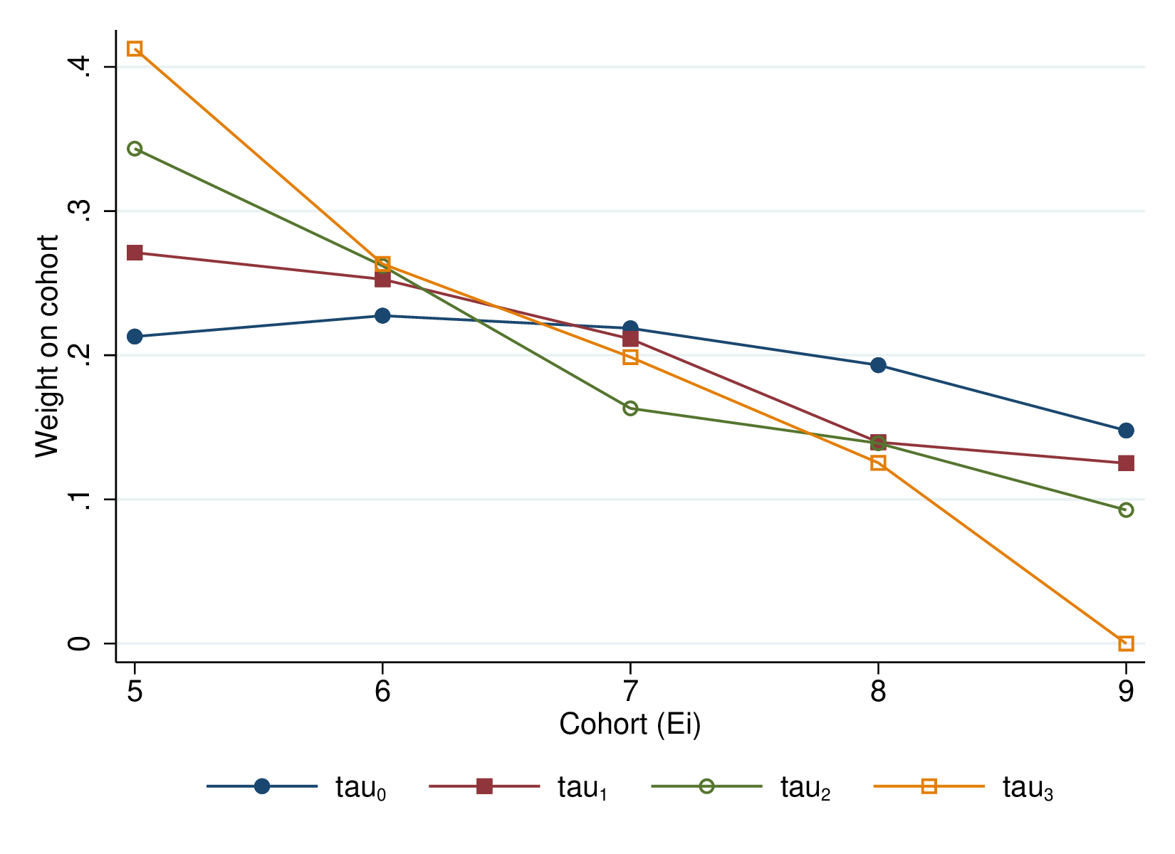
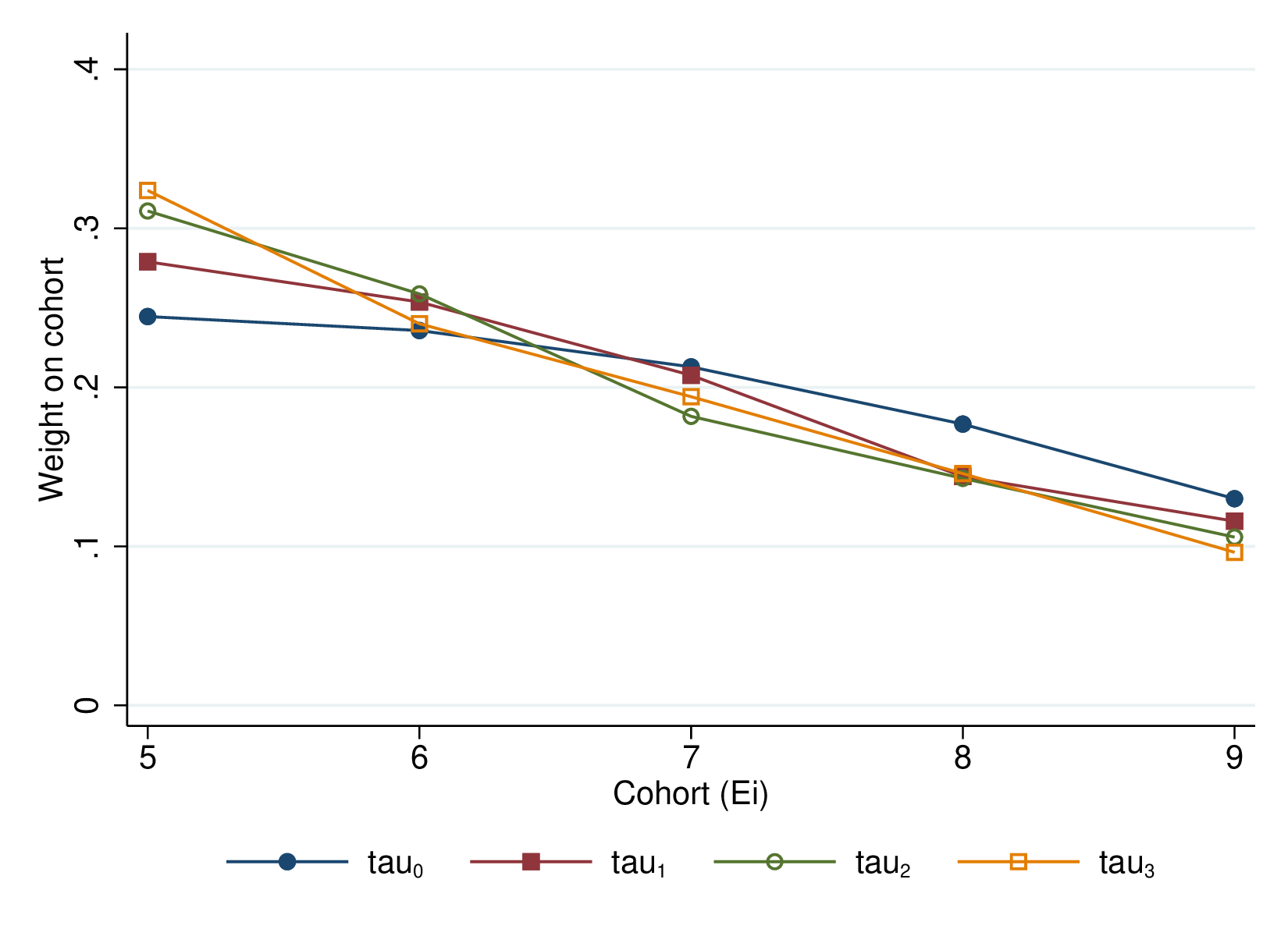
Notes: For the numerical example described in Section A.3 this figure reports the total weight that the $\hat{\tau}_{h}$ estimator from the semi-dynamic specification, for each horizon $h=0,\dots,3$, places on the treated observations from each cohort $e$ observed $h$ periods after treatment. The horizontal axis and the lines correspond to the cohort $e$ and horizon $h$, respectively. Panel A trims the sample to include observations with $K_{it}\in[-4,3]$ only, while Panel B includes all data (but does not report the weights for the coefficients $\tau_{4},\dots,\tau_{7}$). The weights placed by $\hat{\tau}_{h}$ on observations at horizons other than $h$ are not shown.

Figure A2: Efficiency and Bias of Alternative Estimators

Standard deviations under different DGPs
1a: Spherical errors	1b: Heteroskedasticity	1c: AR(1)	1d: Wild clustered
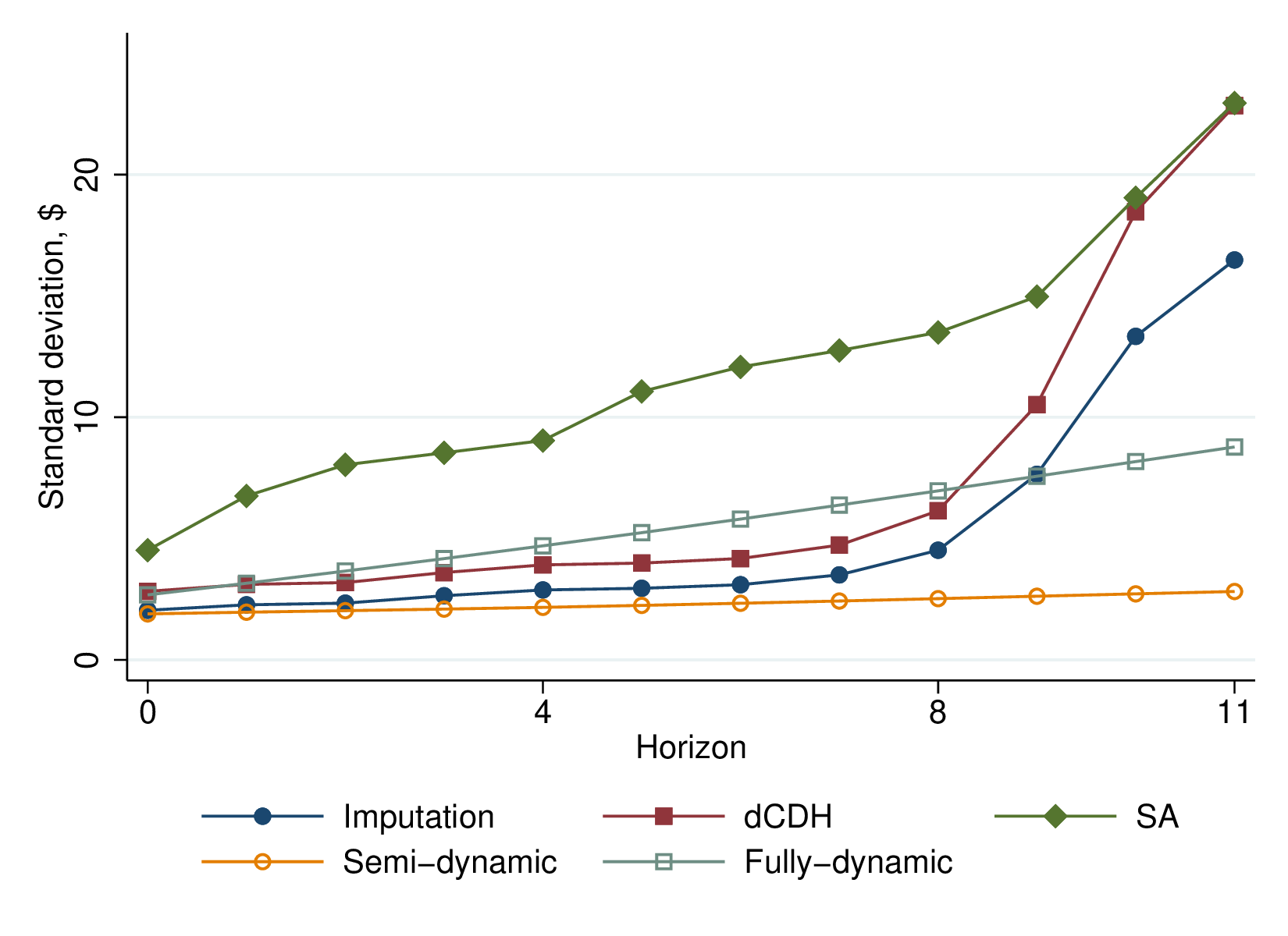
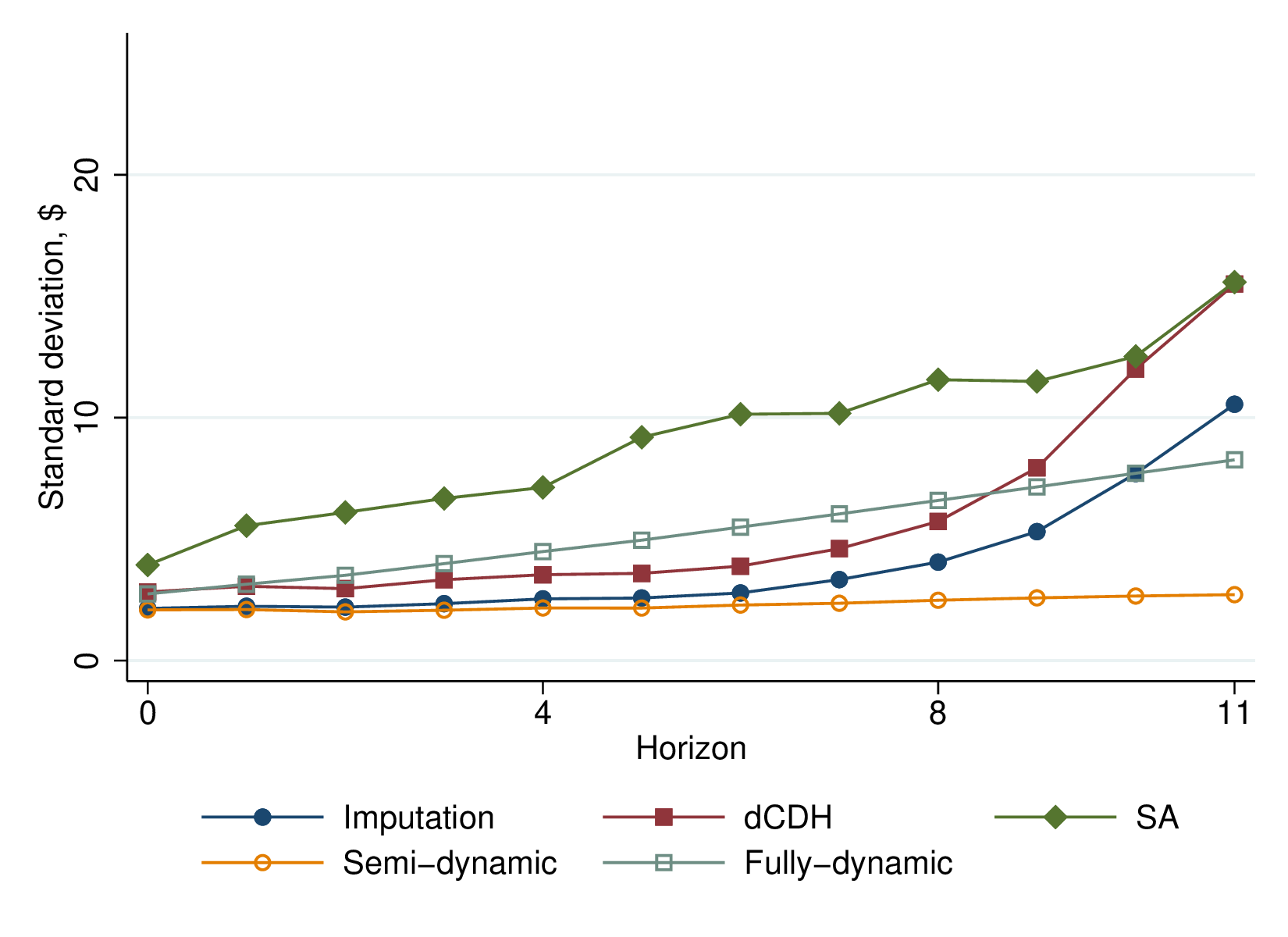
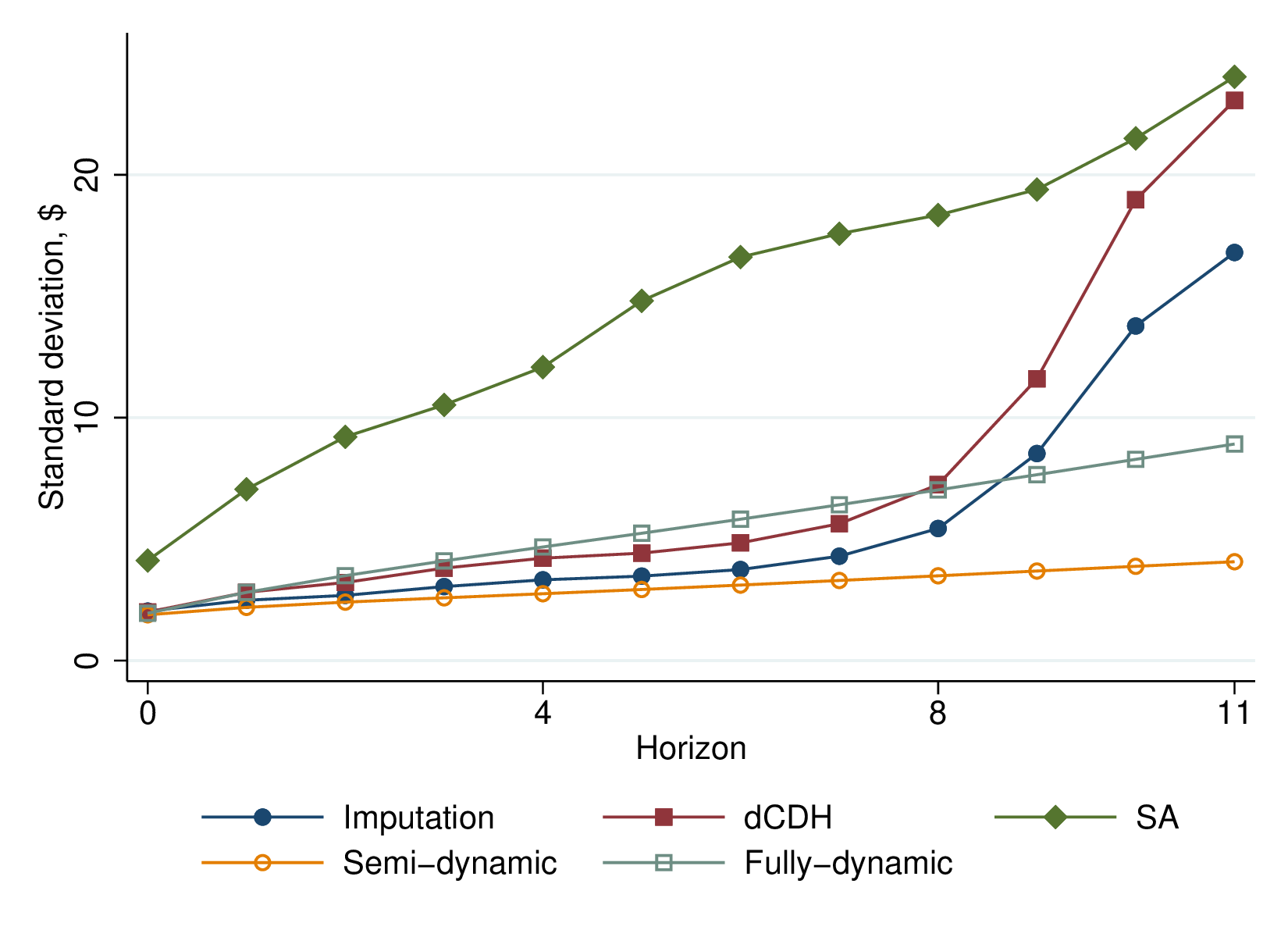
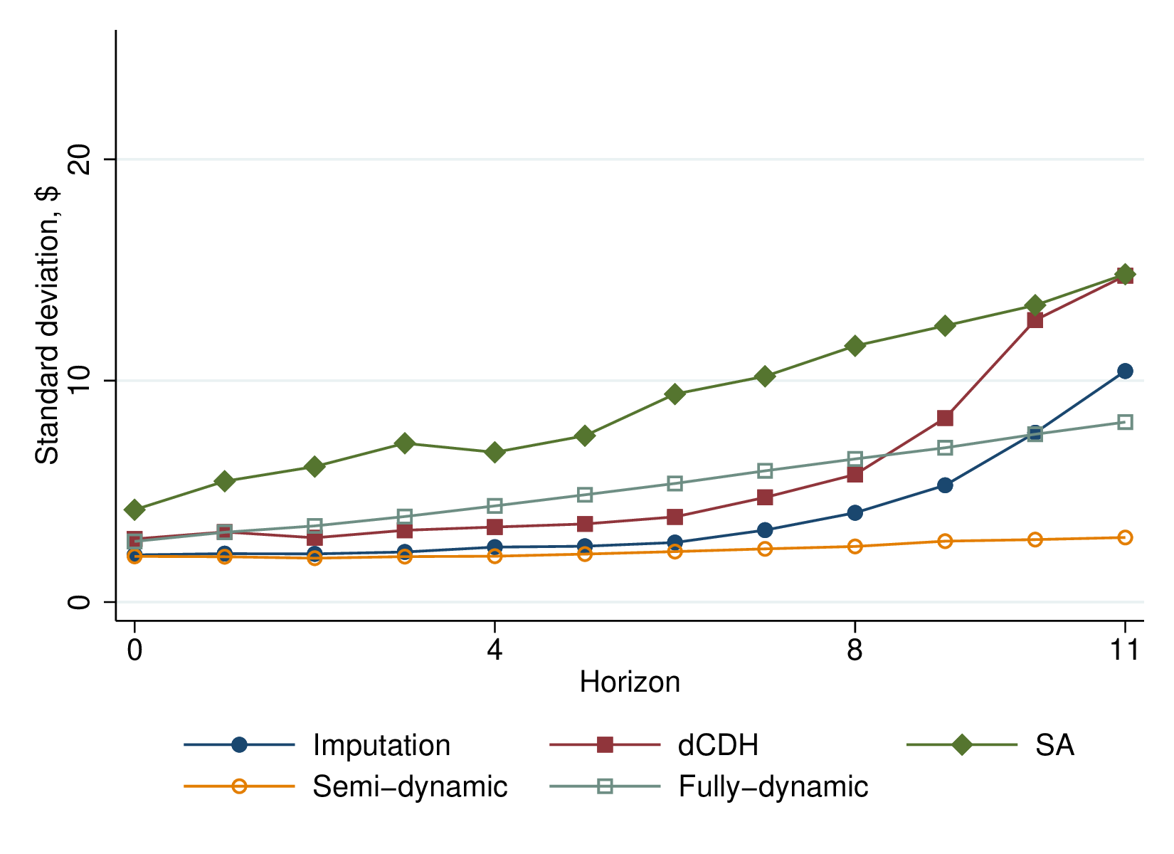
SD relative to the imputation estimator
2a: Spherical errors	2b: Heteroskedasticity	2c: AR(1)	2d: Wild clustered
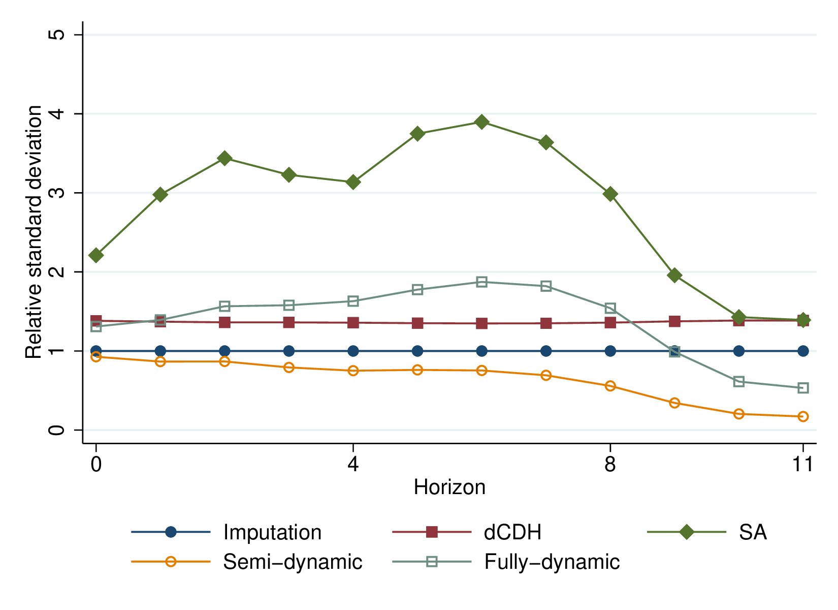
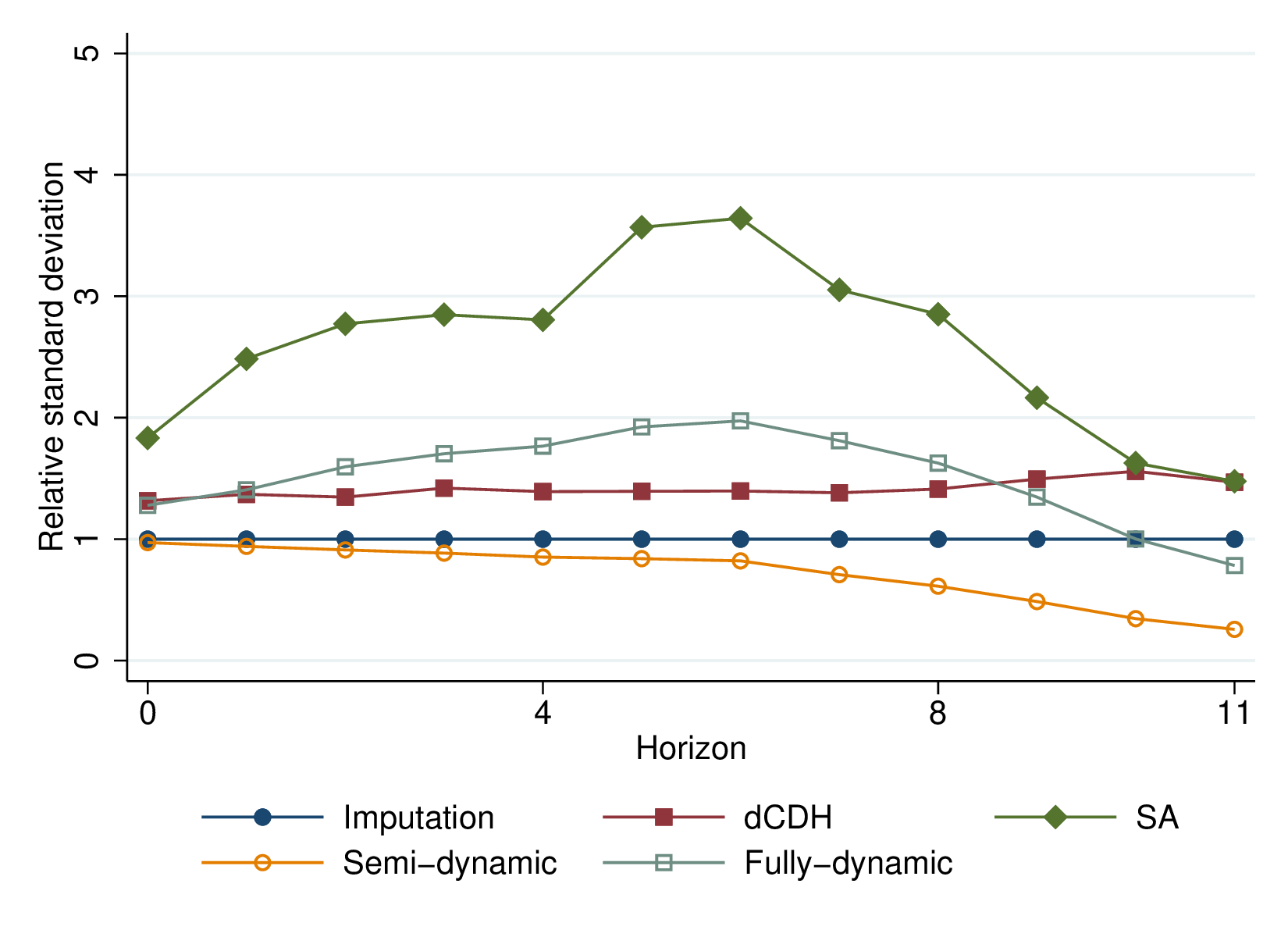
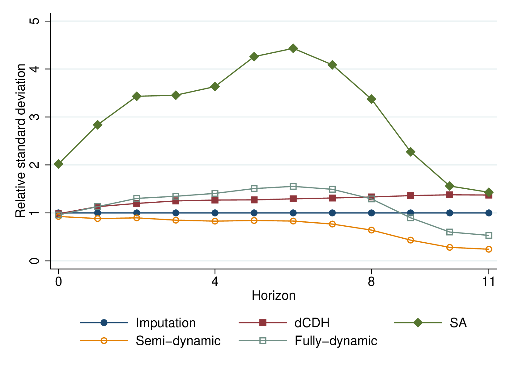
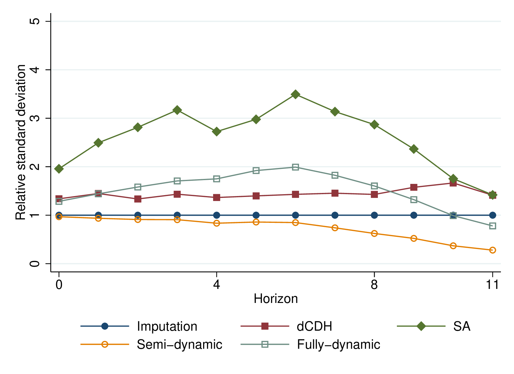
Other simulations
3: Bias	4: RMSE, spherical errors	5: Sensitivity to anticipation	6: Imputation estimator coverage

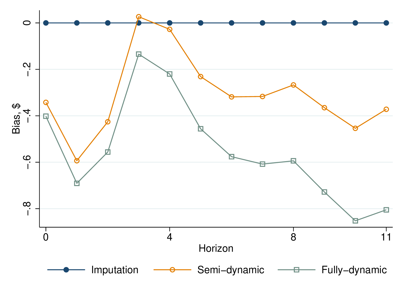
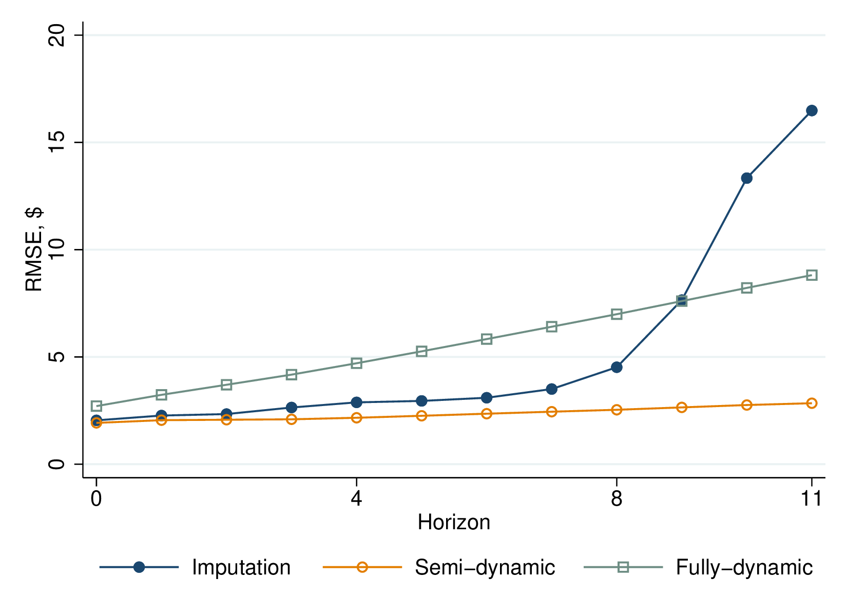
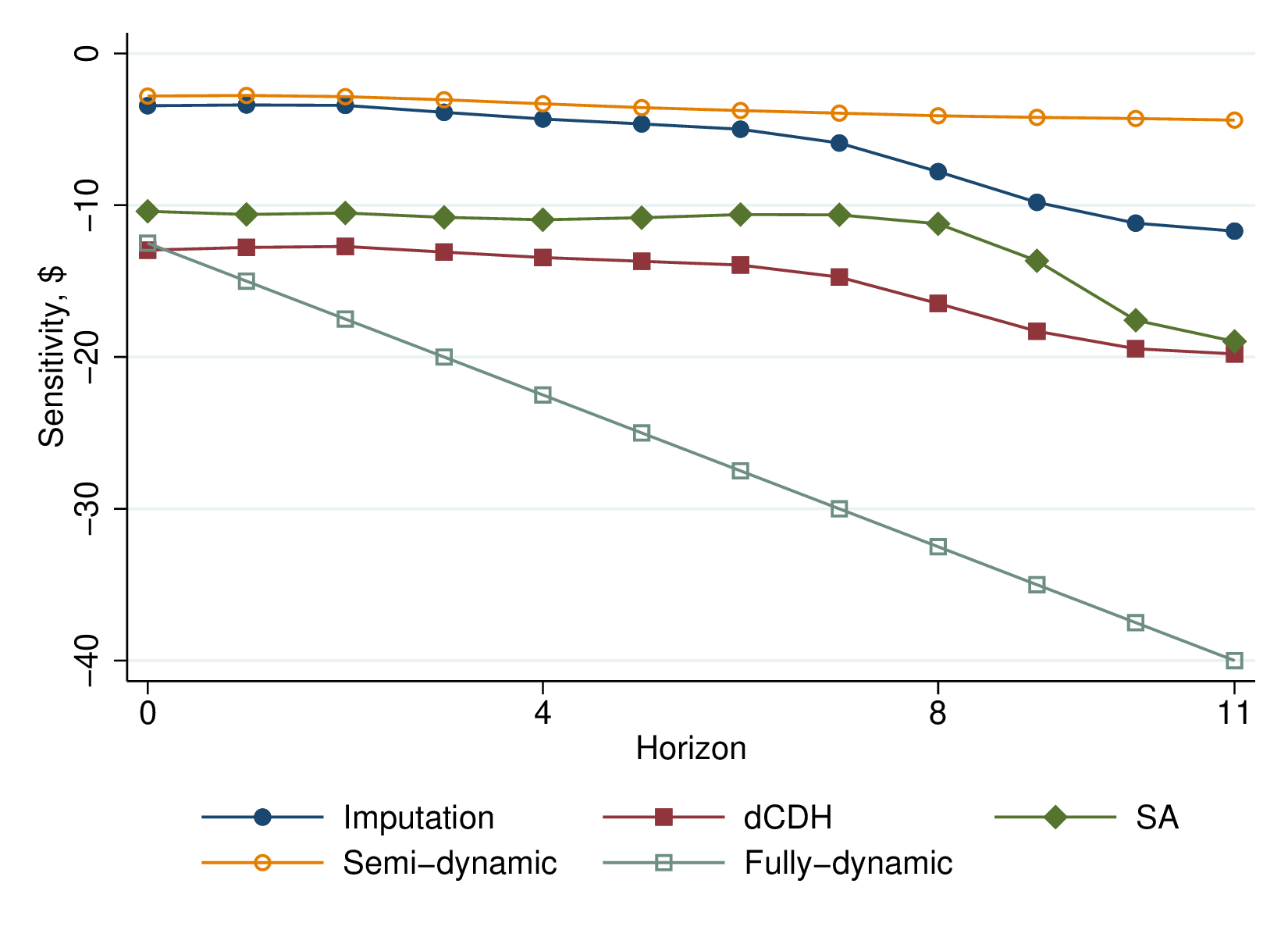
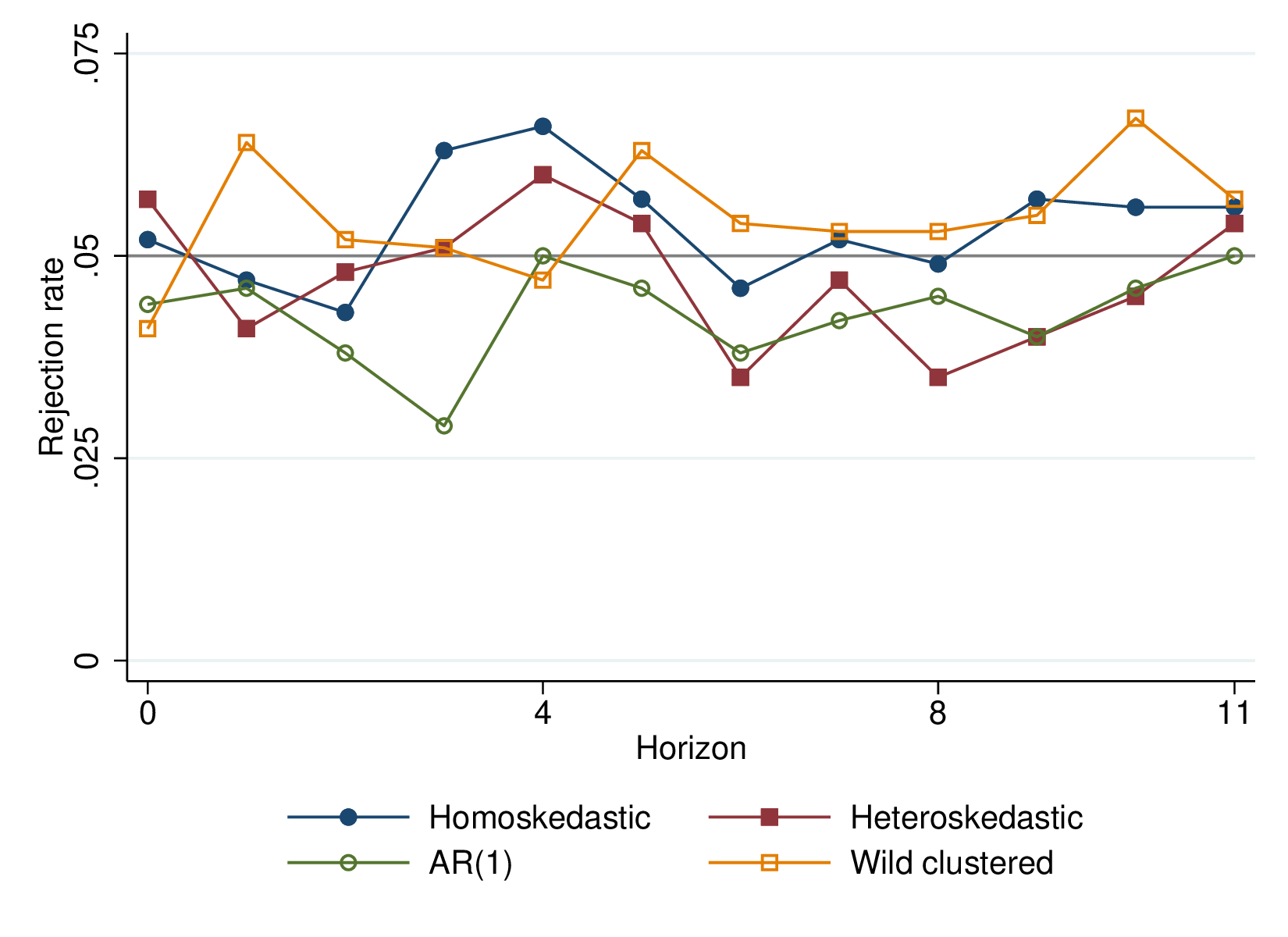
Notes: See Section A.11 for a detailed description of the data-generating processes and reported statistics.

References

- [1] Jaap H. Abbring and Gerard J. Van den Berg “The nonparametric identification of treatment effects in duration models” In Econometrica 71.5, 2003, pp. 1491–1517 DOI: 10.1111/1468-0262.00456
- [2] Joshua Angrist “Estimating the labor market impact of voluntary military service using social security data on military applicants” In Econometrica 66.2, 1998, pp. 249–288 DOI: 10.3386/w5192
- [3] Dmitry Arkhangelsky and Guido W. Imbens “Doubly robust identification for causal panel data models” In The Econometrics Journal 25.3, 2022, pp. 649–674 DOI: 10.1093/ectj/utac019
- [4] Susan Athey et al. “Matrix Completion Methods for Causal Panel Data Models” In Journal of the American Statistical Association 116.536, 2021, pp. 1716–1730 DOI: 10.1080/01621459.2021.1891924
- [5] Andrew C. Baker, David F. Larcker and Charles C.. Wang “How Much Should We Trust Staggered Difference-In-Differences Estimates?” In Journal of Financial Economics 144.2, 2022, pp. 370–395 DOI: https://doi.org/10.1016/j.jfineco.2022.01.004
- [6] Kirill Borusyak and Xavier Jaravel “Revisiting Event Study Designs” In Working Paper, 2018
- [7] Christian Broda and Jonathan A. Parker “The economic stimulus payments of 2008 and the aggregate demand for consumption” In Journal of Monetary Economics 68.S Elsevier, 2014, pp. S20–S36 DOI: 10.1016/j.jmoneco.2014.09.002
- [8] Brantly Callaway, Andrew Goodman-Bacon and Pedro H.C. Sant’Anna “Difference-in-Differences with a Continuous Treatment” In Working paper, 2021 arXiv:2107.02637
- [9] Brantly Callaway and Pedro H.C. Sant’Anna “Difference-in-Differences with Multiple Time Periods and an Application on the Minimum Wage and Employment” In Journal of Econometrics, 2021 arXiv:arXiv:1803.09015v1
- [10] Doruk Cengiz, Arindrajit Dube, Attila Lindner and Ben Zippere “The Effect of Minimum Wages on Low-Wage Jobs” In The Quarterly Journal of Economics, 2019, pp. 1405–1454 DOI: 10.1093/qje/qjz014.Advance
- [11] Sergio Correia “Linear Models with High-dimensional Fixed Effects: An Efficient and Feasible Estimator” In Working Paper, 2017
- [12] Clément de Chaisemartin and Xavier D’Haultfœuille “Fuzzy Differences-in-Differences” In arXiv preprint, 2015
- [13] Clément de Chaisemartin and Xavier D’Haultfœuille “Two-way fixed effects estimators with heterogeneous treatment effects” In American Economic Review 110.9, 2020, pp. 2964–2996 arXiv:arXiv:1803.08807v1
- [14] Clément de Chaisemartin and Xavier D’Haultfœuille “Difference-in-Differences Estimators of Intertemporal Treatment Effects” In Working Paper, 2022 arXiv:arXiv:2007.04267v1
- [15] Marco Di Maggio, Amir Kermani and Kaveh Majlesi “Stock Market Returns and Consumption” In Journal of Finance 75.6, 2020, pp. 3175–3219 DOI: 10.1111/jofi.12968
- [16] John Gardner “Two-stage differences in differences” In Working Paper, 2021
- [17] John Gardner, Neil Thakral, Linh T Tô and Luther Yap “Two-Stage Differences in Differences” In Working Paper, 2023
- [18] Laurent Gobillon and Thierry Magnac “Regional policy evaluation: Interactive fixed effects and synthetic controls” In Review of Economics and Statistics 98.3, 2016, pp. 535–551 DOI: 10.1162/REST_a_00537
- [19] Andrew Goodman-Bacon “Difference-in-differences with variation in treatment timing” In Journal of Econometrics 225.2 Elsevier B.V., 2021, pp. 254–277 DOI: 10.1016/j.jeconom.2021.03.014
- [20] Paulo Guimarães and Pedro Portugal “A simple feasible procedure to fit models with high-dimensional fixed effects” In Stata Journal 10.4, 2010, pp. 628–649 DOI: 10.1177/1536867x1101000406
- [21] Nikolaj A Harmon “Difference-in-Differences and Efficient Estimation of Treatment Effects” In Working paper, 2022
- [22] Hilary W. Hoynes, Diane Whitmore Schanzenbach and Douglas Almond “Long Run Impacts of Childhood Access to the Safety Net” In American Economic Review 106.4, 2016, pp. 903–934 DOI: 10.3386/w18535
- [23] Macartan Humphreys “Bounds on least squares estimates of causal effects in the presence of heterogeneous assignment probabilities” In Working paper, 2009
- [24] Guido W. Imbens and Donald B Rubin “Causal inference in statistics, social, and biomedical sciences” Cambridge University Press, 2015
- [25] David S. Johnson, Jonathan A. Parker and Nicholas S. Souleles “Household expenditure and the income tax rebates of 2001” In American Economic Review 96.5, 2006, pp. 1589–1610 DOI: 10.1257/aer.96.5.1589
- [26] Greg Kaplan and Giovanni L. Violante “A Model of the Consumption Response to Fiscal Stimulus Payments” In Econometrica 82.4, 2014, pp. 1199–1239 DOI: 10.3982/ecta10528
- [27] Greg Kaplan and Giovanni L. Violante “The Marginal Propensity to Consume in Heterogeneous Agent Models” In Annual Review of Economics 14.1, 2022, pp. 747–775 DOI: 10.1146/annurev-economics-080217-053444
- [28] Patrick Kline, Raffaele Saggio and Mikkel Solvsten “Leave-Out Estimation of Variance Components” In Econometrica 88.5, 2020, pp. 1859–1898
- [29] David Laibson, Peter Maxted and Benjamin Moll “A Simple Mapping from MPCs to MPXs” In Working Paper, 2022
- [30] Erich L Lehmann and Joseph P Romano “Testing statistical hypotheses” Springer Science & Business Media, 2006
- [31] Licheng Liu, Ye Wang and Yiqing Xu “A Practical Guide to Counterfactual Estimators for Causal Inference with Time-Series Cross-Sectional Data” In forthcoming American Journal of Political Science, 2022 DOI: 10.2139/ssrn.3555463
- [32] A. MacKinlay “Even Studies in Economics and Finance” In Journal of Economic Literature XXXV, 1997, pp. 13–39 DOI: 10.2307/2729691
- [33] Michelle Marcus and Pedro H.C. Sant’Anna “The role of parallel trends in event study settings: An application to environmental economics” In Journal of the Association of Environmental and Resource Economists 8.2, 2020, pp. 235–275 DOI: 10.1086/711509
- [34] Jacob Orchard, Valerie A. Ramey and Johannes Wieland “Micro MPCs and Macro Counterfactuals: The Case of the 2008 Rebates” In Working Paper, 2023
- [35] Jonathan A. Parker, Nicholas S. Souleles, David S. Johnson and Robert McClelland “Consumer Spending and the Economic Stimulus Payments of 2008” In American Economic Review 103.6, 2013, pp. 2530–2553
- [36] Ashesh Rambachan and Jonathan Roth “A More Credible Approach to Parallel Trends” In The Review of Economic Studies, 2023 DOI: 10.1093/restud/rdad018
- [37] Jonathan Roth “Pretest with Caution: Event-Study Estimates after Testing for Parallel Trends” In American Economic Review: Insights 4.3, 2022, pp. 305–322 DOI: 10.1257/aeri.20210236
- [38] Jonathan Roth and Pedro H.C. Sant’Anna “Efficient Estimation for Staggered Rollout Designs” In Working Paper, 2022 arXiv:2102.01291
- [39] Jonathan Roth and Pedro H.C. Sant’Anna “When Is Parallel Trends Sensitive to Functional Form?” In Econometrica 91.2, 2023, pp. 737–747 DOI: https://doi.org/10.3982/ECTA19402
- [40] Pedro H.C. Sant’Anna and Jun Zhao “Doubly robust difference-in-differences estimators” In Journal of Econometrics 219.1 Elsevier B.V., 2020, pp. 101–122 DOI: 10.1016/j.jeconom.2020.06.003
- [41] Kurt Schmidheiny and Sebastian Siegloch “On event studies and distributed-lags in two-way fixed effects models: Identification, equivalence, and generalization” In Journal of Applied Econometrics 38.5 Wiley Online Library, 2023, pp. 695–713
- [42] James H. Stock and Mark W. Watson “Heteroskedasticity-robust standard errors for fixed effects panel data regression” In Econometrica 76.1, 2008, pp. 155–174 DOI: 10.1111/j.0012-9682.2008.00821.x
- [43] Anton Strezhnev “Semiparametric weighting estimators for multi-period difference-in-differences designs” In Working Paper, 2018
- [44] Liyang Sun and Sarah Abraham “Estimating Dynamic Treatment Effects in Event Studies with Heterogeneous Treatment Effects” In Journal of Econometrics, 2021 arXiv:arXiv:1804.05785v1
- [45] Neil Thakral and Linh T. Tô “Anticipation and Consumption” In Working Paper, 2022
- [46] Justin Wolfers “Did Unilateral Divorce Laws Raise Divorce Rates? A Reconciliation and New Results” In American Economic Review, 2006, pp. 1802–1820
- [47] Jeffrey M Wooldridge “Two-Way Fixed Effects, the Two-Way Mundlak Regression, and Event Study Estimators” In Working Paper, 2021
- [48] Yiqing Xu “Generalized synthetic control method: Causal inference with interactive fixed effects models” In Political Analysis 25.1, 2017, pp. 57–76 DOI: 10.1017/pan.2016.2
- [49] Alexander Bartik and Scott Nelson “Deleting a Signal: Evidence from Pre-Employment Credit Checks” In Working paper, 2021 DOI: 10.2139/ssrn.3498458
- [50] Brantly Callaway and Pedro H.C. Sant’Anna “Difference-in-Differences with Multiple Time Periods and an Application on the Minimum Wage and Employment” In Journal of Econometrics, 2021 arXiv:arXiv:1803.09015v1
- [51] Clément de Chaisemartin and Xavier D’Haultfœuille “Two-way fixed effects estimators with heterogeneous treatment effects” In American Economic Review 110.9, 2020, pp. 2964–2996 arXiv:arXiv:1803.08807v1
- [52] Clément de Chaisemartin and Xavier D’Haultfœuille “Difference-in-Differences Estimators of Intertemporal Treatment Effects” In Working Paper, 2022 arXiv:arXiv:2007.04267v1
- [53] Paul Goldsmith-Pinkham and Guido W Imbens “Social Networks and the Identification of Peer Effects” In Journal of Business & Economic Statistics 31.3 Taylor & Francis, 2013, pp. 253–264
- [54] Paulo Guimarães and Pedro Portugal “A simple feasible procedure to fit models with high-dimensional fixed effects” In Stata Journal 10.4, 2010, pp. 628–649 DOI: 10.1177/1536867x1101000406
- [55] Nikolaj A Harmon “Difference-in-Differences and Efficient Estimation of Treatment Effects” In Working paper, 2022
- [56] Patrick Kline, Raffaele Saggio and Mikkel Solvsten “Leave-Out Estimation of Variance Components” In Econometrica 88.5, 2020, pp. 1859–1898
- [57] James G. Mackinnon and Halbert White “Some heteroskedasticity-consistent covariance matrix estimators with improved finite sample properties” In Journal of Econometrics 29, 1985, pp. 305–325
- [58] Michelle Marcus and Pedro H.C. Sant’Anna “The role of parallel trends in event study settings: An application to environmental economics” In Journal of the Association of Environmental and Resource Economists 8.2, 2020, pp. 235–275 DOI: 10.1086/711509
- [59] Conrad Miller “The Persistent Effect of Temporary Affirmative Action” In American Economic Journal: Applied Economics 9.3, 2017, pp. 152–190
- [60] Liyang Sun and Sarah Abraham “Estimating Dynamic Treatment Effects in Event Studies with Heterogeneous Treatment Effects” In Journal of Econometrics, 2021 arXiv:arXiv:1804.05785v1
- [61] Aad W. van der Vaart “Asymptotic statistics” Cambridge university press, 2000
- [62] Jeffrey M Wooldridge “Two-Way Fixed Effects, the Two-Way Mundlak Regression, and Event Study Estimators” In Working Paper, 2021