Hadronic light-by-light contribution to the muon $g-2$
from holographic QCD with massive pions

Abstract

We extend our previous calculations of the hadronic light-by-light scattering contribution to the muon anomalous magnetic moment in holographic QCD to models with finite quark masses and a tower of massive pions. Analysing the role of the latter in the Wess-Zumino-Witten action, we show that the Melnikov-Vainshtein short-distance constraint is satisfied solely by the summation of contributions from the infinite tower of axial vector meson contributions. There is also an enhancement of the asymptotic behavior of pseudoscalar contributions when their infinite tower of excitations is summed, but this leads only to subleading contributions for the short-distance constraints on light-by-light scattering. We also refine our numerical evaluations, particularly in the pion and $a_{1}$ sector, which corroborates our previous findings of contributions from axial vector mesons that are significantly larger than those adopted for the effects of axials and short-distance constraints in the recent White Paper on the Standard Model prediction for $(g-2)_{\mu}$.

I Introduction

Recently, the Muon $g-2$ Collaboration at Fermilab Muong-2:2021ojo has confirmed the long-standing discrepancy between the E821/BNL measurement Muong-2:2006rrc of the anomalous magnetic moment of the muon Jegerlehner:2017gek and the Standard Model prediction, which according to the White Paper (WP) of the Muon $g-2$ Theory Initiative Aoyama:2020ynm is below the combined experimental value by an amount of $\Delta a_{\mu}=\Delta(g-2)_{\mu}/2=251(59)\times 10^{-11}$.

While QED Aoyama:2012wk ; *Aoyama:2017uqe; *Aoyama:2019ryr and electroweak effects Czarnecki:2002nt ; Gnendiger:2013pva appear to be fully under control, the theoretical uncertainty is dominated by hadronic effects Melnikov:2003xd ; Prades:2009tw ; Kurz:2014wya ; Colangelo:2014qya ; Pauk:2014rta ; Davier:2017zfy ; Masjuan:2017tvw ; Colangelo:2017fiz ; Keshavarzi:2018mgv ; Colangelo:2018mtw ; Hoferichter:2019gzf ; Davier:2019can ; Keshavarzi:2019abf ; Hoferichter:2018dmo ; *Hoferichter:2018kwz; Gerardin:2019vio ; Bijnens:2019ghy ; Colangelo:2019lpu ; Colangelo:2019uex ; Danilkin:2019mhd ; Blum:2019ugy ; Chao:2021tvp . The largest contribution by far is the hadronic vacuum polarization, where a recent lattice calculation Borsanyi:2020mff has challenged the WP result, albeit by producing tensions in other quantities Crivellin:2020zul ; Keshavarzi:2020bfy ; Colangelo:2020lcg – an issue which further lattice calculations as well as new experimental results on hadronic cross sections should resolve in the near future. The second largest uncertainty comes from hadronic light-by-light scattering (HLBL) Danilkin:2019mhd , which also needs improvements in view of the expected reductions of experimental errors by the ongoing experiment at Fermilab and a new one in preparation at J-PARC Abe:2019thb .

At the low energies relevant for the evaluation of $a_{\mu}$, the HLBL amplitude is dominated by the two-photon coupling of the pion, where the transition form factors (TFF) needed to evaluate the pion pole contribution has been computed with satisfying accuracy in data-driven approaches Masjuan:2017tvw ; Hoferichter:2018dmo ; *Hoferichter:2018kwz which are also in agreement with results from lattice QCD Gerardin:2019vio . Among the many additional low-energy contributions, those contributed by axial vector mesons are currently the ones involving the largest uncertainties due to insufficient experimental data. Axial vector mesons also play a crucial role in connecting the HLBL amplitude at low energies to short-distance constraints (SDCs), in particular the one derived by Melnikov and Vainshtein (MV) Melnikov:2003xd using the non-renormalization theorem for the vector-vector-axial-vector (VVA) correlator and the axial anomaly, as has been clarified by holographic models of QCD (hQCD) Leutgeb:2019gbz ; Cappiello:2019hwh , which are the first hadronic models to implement fully the constraints Knecht:2020xyr ; Masjuan:2020jsf imposed by the axial anomaly in the chiral limit.

Away from the chiral limit, also excited pseudoscalars couple to the axial vector current and thus to the axial anomaly. In Colangelo:2019lpu ; Colangelo:2019uex a Regge model for excited pseudoscalars has been constructed to satisfy the longitudinal SDCs (LSDCs) and to estimate the corresponding contributions to $a_{\mu}$. In this paper we employ the simplest hard-wall AdS/QCD model that is capable of satisfying at the same time the leading-order (LO) perturbative QCD (pQCD) constraints on the vector correlator and the low-energy parameters provided by the pion decay constant $f_{\pi}$ and the mass of the $\rho$ meson, introduced in Erlich:2005qh ; DaRold:2005mxj ; *DaRold:2005vr and called HW1 in Cappiello:2010uy ; Leutgeb:2019zpq ; Leutgeb:2019gbz , using here its generic form with finite quark masses (albeit in the simplest version of uniform quark masses). This allows us to study the role of massive pions in the axial anomaly and in the longitudinal SDCs. We find that in hQCD there is in fact a certain enhancement of the asymptotic behavior when summing the infinite tower of pseudoscalars compared to the behavior of individual contributions, but within the allowed range of parameters of hQCD this is insufficient to let pseudoscalars contribute to the leading terms of the longitudinal SDCs; the latter are determined by the infinite tower of axial vector mesons alone, in agreement with the expectation expressed in Cappiello:2019hwh .

Moreover, we evaluate and assess a set of massive hard-wall AdS/QCD models with regard to their predictions for the pseudoscalar and axial-vector TFFs and the resulting contributions to $a_{\mu}$, also allowing for adjustments at high energies to account for next-to-leading (NLO) pQCD corrections. The results for the single and double-virtual pion TFFs agree perfectly with those of the data-driven dispersive results of Ref. Hoferichter:2018kwz , in particular when a 10% reduction of the asymptotic limit is applied. The shape of the axial vector TFF is consistent with L3 results for the $f_{1}(1285)$ axial vector meson Achard:2001uu ; the magnitude is above experimental values, but becomes compatible after such reductions. While hQCD is clearly only a toy model for real QCD, this success after a fit of a minimal set of low-energy parameters seems to make it also interesting as a phenomenological model (which may be further improved by using a modified background geometry and other refinements Ghoroku:2005vt ; Karch:2006pv ; Gursoy:2007cb ; *Gursoy:2007er).

Numerically, the axial vector contributions are close to our previous results for the HW1 model in the chiral limit (they even tend to increase with finite quark masses), and they are thus significantly larger than estimated in the WP Aoyama:2020ynm . Interestingly enough, a new complete lattice calculation which claims comparable errors Chao:2021tvp has obtained somewhat larger values of $a_{\mu}^{\mathrm{HLBL}}$ than the WP Aoyama:2020ynm , which could also be indicative of larger contributions from the axial vector meson sector.

The contributions from the excited pseudoscalars are numerically much smaller than those from axial vector mesons. They are present also in the chiral HW1 model, where they decouple from the axial vector current and the axial anomaly, but not from low-energy photons. However, the first excited pion mode has a two-photon coupling that is significantly above the experimental constraint deduced in Colangelo:2019uex . Nevertheless, the contribution of the first few excited modes together is smaller than those of the Regge model of Colangelo:2019lpu ; Colangelo:2019uex , which is compatible with known experimental constraints. This model was, however, not meant primarily as a phenomenological model for estimating the contributions of excited pseudoscalars but rather as a model for estimating the effects of the longitudinal SDCs, which according to the hQCD models are instead provided by the axial vector mesons. As far as these effects are concerned, our present results are not far above the estimates obtained in Colangelo:2019lpu ; Colangelo:2019uex ; Ludtke:2020moa ; Colangelo:2021nkr ; all are significantly below the estimates obtained with the so-called MV model Melnikov:2003xd , where the ground-state pion contribution is modified.

This paper is organized as follows. In Sec. II we review hQCD with an anti-de Sitter (AdS) background that is cut off by a hard wall and where in addition to flavor gauge fields a bifundamental scalar bulk field encodes the chiral condensates with or without finite quark masses. In addition to the boundary conditions considered originally in Ref. Erlich:2005qh ; DaRold:2005mxj where vector and axial vector gauge fields are treated equally (HW1), we also consider the other set of admissible boundary conditions that appear in models without a bifundamental scalar, the Hirn-Sanz (HW2) model Hirn:2005nr and the top-down hQCD model of Sakai and Sugimoto Sakai:2004cn ; Sakai:2005yt . (This modification of the HW1 model will be referred to as HW3.) As has been pointed out in Domenech:2010aq , this has the advantage of removing infrared boundary terms in the Chern-Simons action that in the HW1 model need to be subtracted by hand Grigoryan:2007wn . Additionally we consider the generalization of different scaling dimensions for quark masses and chiral condensates proposed in Domenech:2010aq , which permits to fit the mass of the first excited pion or the lowest axial vector meson. In Sec. III, we analyse the consequences of the axial anomaly in the HW models, in particular the role of excited pseudoscalars, as encoded by the bulk Chern-Simons action for the five-dimensional gauge fields. In Sec. IV we study SDCs on TFFs and the HLBL scattering amplitude, showing analytically that the MV-SDC is always saturated by axial vector mesons, while the symmetric longitudinal SDC is fulfilled to 81%. Within the bounds of allowed scaling dimensions for the bulk bifundamental scalar, the infinite tower of excited pseudoscalar cannot change this. Finally in Sec. V we evaluate the set of massive HW models numerically, comparing the resulting masses, decay constants, and TFFs with empirical data, before calculating the corresponding contributions to $a_{\mu}$.

II Hard-wall AdS/QCD models with finite quark masses

In the hard-wall AdS/QCD models of Ref. Erlich:2005qh ; DaRold:2005mxj ; Hirn:2005nr , the background geometry is chosen as pure anti-de Sitter with metric

$$ds^{2}=z^{-2}(\eta_{\mu\nu}dx^{\mu}dx^{\nu}-dz^{2}),$$ (1)

with a conformal boundary at $z=0$. Confinement is implemented by a cutoff at some finite value of the radial coordinate $z_{0}$, where boundary conditions for the five-dimensional fields are imposed.

Left and right chiral quark currents are dual to five-dimensional flavor gauge fields, whose action is given by a Yang-Mills part

$$S_{\rm YM}=-\frac{1}{4g_{5}^{2}}\int d^{4}x\int_{0}^{z_{0}}dz\,\sqrt{-g}\,g^{PR}g^{QS}\,\text{tr}\left(\mathcal{F}^{\mathrm{L}}_{PQ}\mathcal{F}^{\mathrm{L}}_{RS}+\mathcal{F}^{\mathrm{R}}_{PQ}\mathcal{F}^{\mathrm{R}}_{RS}\right),$$ (2)

where $P,Q,R,S=0,\dots,3,z$ and $\mathcal{F}_{MN}=\partial_{M}\mathcal{B}_{N}-\partial_{N}\mathcal{B}_{M}-i[\mathcal{B}_{M},\mathcal{B}_{N}]$, and a Chern-Simons action $S_{\rm CS}=S_{\rm CS}^{\mathrm{L}}-S_{\rm CS}^{\mathrm{R}}$ with (in differential form notation)

$$S_{\rm CS}^{\mathrm{L,R}}=\frac{N_{c}}{24\pi^{2}}\int\text{tr}\left(\mathcal{B}\mathcal{F}^{2}-\frac{i}{2}\mathcal{B}^{3}\mathcal{F}-\frac{1}{10}\mathcal{B}^{5}\right)^{\mathrm{L,R}},$$ (3)

up to a potential subtraction of boundary terms at $z_{0}$ to be discussed below.

As dual field for the scalar quark bilinear operator, a bi-fundamental bulk scalar Erlich:2005qh ; DaRold:2005mxj $X$, parametrized as Abidin:2009aj

$$X=e^{i\pi^{a}(x,z)t^{a}}[{\textstyle\frac{1}{2}}v(z)]e^{i\pi^{a}(x,z)t^{a}},$$ (4)

is introduced, with action

$$S_{X}=\int d^{4}x\int_{0}^{z_{0}}dz\,\sqrt{-g}\,\text{tr}\left(|DX|^{2}-M_{X}^{2}|X|^{2}\right),$$ (5)

where $D_{M}X=\partial_{M}X-i\mathcal{B}_{M}^{\mathrm{L}}X+iX\mathcal{B}_{M}^{\mathrm{R}}$. The five-dimensional mass term is determined by the scaling dimension of the chiral-symmetry breaking order parameter $\bar{q}_{L}q_{R}$ of the boundary theory. With $M_{X}^{2}=-3$, one obtains vacuum solutions $v(z)=M_{q}z+\Sigma\,z^{3}$, where $M_{q}$ and $\Sigma$ are model parameters related to the quark mass matrix and the quark condensate. Following Ref. Domenech:2010aq we shall also consider generalizations away from $M_{X}^{2}=-3$, where

$$v(z)=M_{q}z_{0}(z/z_{0})^{\Delta^{-}}+\Sigma\,z_{0}^{3}(z/z_{0})^{\Delta^{+}}$$ (6)

with

$$\Delta^{\pm}=2\pm\sqrt{4+M_{X}^{2}}\equiv 2\pm\alpha.$$ (7)

In the original hard-wall model of Ref. Erlich:2005qh ; DaRold:2005mxj (HW1), chiral symmetry preserving boundary conditions are employed at the infrared cutoff, $\mathcal{F}^{\mathrm{L,R}}_{z\mu}(z_{0})=0$, whereas in the model of Hirn and Sanz Hirn:2005nr (called HW2 in Cappiello:2010uy ; Leutgeb:2019zpq ; Leutgeb:2019gbz ) chiral symmetry is broken through $(\mathcal{B}^{\mathrm{L}}_{\mu}-\mathcal{B}^{\mathrm{R}}_{\mu})(z_{0})=0$ and $(\mathcal{F}^{\mathrm{L}}_{z\mu}+\mathcal{F}^{\mathrm{R}}_{z\mu})(z_{0})=0$ without the introduction of a bi-fundamental scalar. These latter conditions arise naturally in the top-down holographic chiral model of Sakai and Sugimoto Sakai:2004cn ; Sakai:2005yt with flavor gauge fields residing on flavor branes separated by an extra dimension at the boundary but connecting in the bulk. In Domenech:2010aq , it was proposed to use such symmetry breaking boundary conditions also in the presence of symmetry breaking by a bifundamental scalar, because it avoids infrared boundary contributions from the CS action. This variant of the HW1 model will be termed HW3 in the following.

In both, the HW1 and the HW3 model, chiral symmetry can be broken additionally by finite quark masses. In the present paper, we shall only consider the flavor symmetric case, where both $M_{q}$ and $\Sigma$ are proportional to the unit matrix. For both models we will also consider generalizations away from $M_{X}^{2}=-3$, which, as Ref. Domenech:2010aq has found, allows the HW3 model to fit simultaneously the masses of the lightest and the first excited pion. As shown in Appendix A, all these models lead to a Gell-Mann–Oakes–Renner (GOR) relation in the limit of small quark masses, to wit,

$$f_{\pi}^{2}m_{\pi}^{2}=2\alpha M_{q}\Sigma\quad\mbox{for}\;M_{q}\ll\Sigma z_{0}^{2}\propto\Sigma/m_{\rho}^{2},$$ (8)

where $\alpha=1$ for the standard choice $M_{X}^{2}=-3$, and $0<\alpha<2$ for the admissible generalizations Domenech:2010aq $-4<M_{X}^{2}<0$.

II.1 Vector sector

As long as flavor symmetry is in place, vector mesons, which appear in the mode expansion of $V_{\mu}=(\mathcal{B}^{L}_{\mu}+\mathcal{B}^{R}_{\mu})/2$, have (for all hard-wall models considered here) quark-mass independent holographic wave functions given by

$$\partial_{z}\left[\frac{1}{z}\partial_{z}\psi_{n}(z)\right]+\frac{1}{z}M_{n}^{2}\psi_{n}(z)=0$$ (9)

with boundary conditions $\psi_{n}(0)=\psi^{\prime}_{n}(z_{0})=0$. This is solved by $\psi_{n}(z)\propto zJ_{1}(M_{n}z)$ with $M_{n}$ determined by the zeros of the Bessel function $J_{0}$, denoted by $\gamma_{0,n}$. With normalization $\int_{0}^{z_{0}}dz\,z^{-1}\psi_{n}(z)^{2}=1$ we have

$$\psi_{n}(z)=\sqrt{2}\frac{zJ_{1}(\gamma_{0,n}z/z_{0})}{z_{0}J_{1}(\gamma_{0,n})}$$ (10)

and canonically normalized vector meson fields $v_{\mu}(x)$ in the mode expansion $V_{\mu}^{a}=g_{5}\sum_{n=1}^{\infty}v_{\mu}^{a}(x)\psi_{n}(z)$.

Identifying $M_{1}=\gamma_{0,1}/z_{0}=m_{\rho}=775$ MeV, we obtain

$$z_{0}=\gamma_{0,1}/m_{\rho}=3.103\,\text{GeV}^{-1}.$$ (11)

The vector bulk-to-boundary propagator is obtained by replacing $M_{n}^{2}$ by $q^{2}=-Q^{2}$ and the boundary conditions by $\mathcal{J}(Q,0)=1$ and $\partial_{z}\mathcal{J}(Q,z_{0})=0$. This gives

$$\mathcal{J}(Q,z)=Qz\left[K_{1}(Qz)+\frac{K_{0}(Qz_{0})}{I_{0}(Qz_{0})}I_{1}(Qz)\right]=\sum_{n=1}^{\infty}\frac{g_{5}F_{n}^{V}\psi_{n}(z)}{Q^{2}+M_{n}^{2}},$$ (12)

where $F_{n}^{V}=|\psi_{n}^{\prime}(\epsilon)/(g_{5}\epsilon)|$ is the decay constant of $v_{n}(x)$,

$$\langle 0|J_{\mu}^{a}(0)|v_{n}^{b}(q,\lambda)\rangle=F_{n}^{V}\varepsilon_{\mu}(q,\lambda)\delta^{ab}.$$ (13)

Requiring that the vector current two-point function matches the leading-order pQCD result Erlich:2005qh ,

$$\Pi_{V}(Q^{2})=-\frac{1}{g_{5}^{2}Q^{2}}\left(\frac{1}{z}\partial_{z}\mathcal{J}(Q,z)\right)\Big{|}_{z\to 0}=-\frac{N_{c}}{24\pi^{2}}\ln Q^{2},$$ (14)

determines $g_{5}^{2}=12\pi^{2}/N_{c}$.

The simpler Hirn-Sanz (HW2) model Hirn:2005nr , which does not include the scalar $X$, cannot set $g_{5}^{2}$ to the value required by pQCD, when the mass of the rho meson and the pion decay constant is matched to experiment (as we shall do throughout).

II.2 Axial sector

Following the notation of Ref. Abidin:2009aj , the five-dimensional Lagrangian contains the following quadratic terms for the axial gauge field $A_{M}=(\mathcal{B}^{L}_{M}-\mathcal{B}^{R}_{M})/2$ and the pseudoscalar $\pi$,

$$\mathcal{L}_{axial}=-\frac{1}{4g_{5}^{2}z}(\partial_{M}A_{N}-\partial_{N}A_{M})^{2}+\frac{\beta(z)}{2g_{5}^{2}z}(\partial_{M}\pi-A_{M})^{2},\qquad\beta(z)=g_{5}^{2}v^{2}/z^{2},$$ (15)

where five-dimensional indices are implicitly contracted with a five-dimensional Minkowski metric $\eta^{MN}$ (mostly minus).

Axial vector mesons are contained in $A_{\mu}^{\perp}=g_{5}\sum_{n=1}^{\infty}a_{\mu}^{(n)}(x)\psi_{n}^{A}(z)$ with the holographic wave functions subject to

$$\partial_{z}\left[\frac{1}{z}\partial_{z}\psi^{A}_{n}(z)\right]+\frac{1}{z}\left[M_{A,n}^{2}-\beta(z)\right]\psi^{A}_{n}(z)=0,$$ (16)

which is different than (9) when $v\not=0$ and so gives a different mass spectrum even when vector and axial vector fields have identical boundary conditions, as is the case in the HW1 model. In the HW3 model, chiral symmetry is additionally broken by the Dirichlet boundary condition $\psi_{n}^{A}(z_{0})_{\mathrm{HW3}}=0$.

In the holographic gauge $A_{z}=0$, the pseudoscalar $\pi$ mixes with the longitudinal part of the axial vector gauge field denoted by $A_{\mu}^{\parallel}=\partial_{\mu}\phi$,

$$\mathcal{L}_{axial}\supset\frac{1}{2g_{5}^{2}z}(\partial_{\mu}\partial_{z}\phi)^{2}+\frac{1}{2g_{5}^{2}z}\beta(z)(\partial_{\mu}\pi-\partial_{\mu}\phi)^{2}-\frac{1}{2g_{5}^{2}z}\beta(z)(\partial_{z}\pi)^{2}.$$ (17)

Alternatively, one may decouple $A_{\mu}$ from $A_{z}$ and $\pi$ by adding the $R_{\xi}$ gauge fixing term Domenech:2010aq

$$\mathcal{L}_{R_{\xi}}=-\frac{1}{2\xi zg_{5}^{2}}\left[\partial_{\mu}A^{\mu}-\xi z\partial_{z}\left(\frac{1}{z}A_{z}\right)+\xi\beta\pi\right]^{2}.$$ (18)

Taking the $\xi\to\infty$ limit imposes the unitary gauge, which fixes

$$z\partial_{z}\left(\frac{1}{z}A_{z}^{\mathrm{U}}\right)=\beta\pi^{\mathrm{U}}.$$ (19)

In the unitary gauge, $A_{\mu}^{\mathrm{U}}$ is a simple Proca field, and the relation to the fields in the holographic gauge (the latter written without label) are $A_{M}^{\mathrm{U}}=A_{M}-\partial_{M}\phi$, $\pi^{\mathrm{U}}=\pi-\phi$ with $A_{\mu}^{\parallel\mathrm{U}}=0$ and $A_{z}^{\mathrm{U}}=-\partial_{z}\phi$.

The equations of motion for $\phi$ and $\pi$ read

$$\partial_{z}\left(\frac{1}{z}\partial_{z}\phi\right)+\frac{\beta(z)}{z}\left(\pi-\phi\right) = 0,$$ (20)

$$\partial_{z}\left(\frac{\beta(z)}{z}\partial_{z}\pi\right)+\frac{\beta(z)}{z}q^{2}\left(\pi-\phi\right)=0.$$ (21)

Defining $y=\partial_{z}\phi/z$, one can combine these coupled equations into a single second order differential equation Kwee:2007dd ; Abidin:2009aj

$$(L+q^{2})y:=\frac{\beta(z)}{z}\partial_{z}\left(\frac{z}{\beta(z)}\partial_{z}y\right)-\beta(z)y+q^{2}y=0.$$ (22)

The modes for $\pi$ follow from (20) and (21) which imply

$$\partial_{z}y=\frac{\beta(z)}{z}\left(\phi-\pi\right)$$ (23)

and

$$\partial_{z}\pi=\frac{q^{2}}{\beta(z)}zy.$$ (24)

The boundary conditions at $z=\epsilon\to 0$ are $\phi_{S}(q,\epsilon)=0$, $\pi_{S}(q,\epsilon)=-1$ for the non-normalizable profile functions, and $\phi_{n}(\epsilon)=0$, $\pi_{n}(\epsilon)=0$ for the normalizable modes. This implies

$$\left.\frac{z}{\beta(z)}\partial_{z}y_{S}(q,z)\right|_{z=\epsilon}=1,\quad\left.\frac{z}{\beta(z)}\partial_{z}y_{n}(z)\right|_{z=\epsilon}=0.$$ (25)

At the infrared boundary $z=z_{0}$ there are two possible choices which eliminate the boundary term in the axial part of the action

$$\frac{1}{2g_{5}^{2}z_{0}}\left(q^{2}\phi\partial_{z}\phi-\beta\pi\partial_{z}\pi\right)_{z=z_{0}}=\frac{q^{2}}{2g_{5}^{2}}y(z_{0})\left[\phi(z_{0})-\pi(z_{0})\right].$$ (26)

In the HW1 model, one has Neumann boundary conditions at $z=z_{0}$ for all gauge fields, and therefore on $\phi$; (26) is then cancelled by requiring $y(z_{0})=0$. In the HW3 model, where the axial gauge field has Dirichlet boundary conditions, one chooses instead $\partial_{z}y|_{z=z_{0}}=0$, which through (23) implies $[\phi(z_{0})-\pi(z_{0})]=0$. The HW2/HW3 boundary condition $A_{\mu}(z_{0})=0$ thus only applies to $A^{\perp}_{\mu}(z_{0})=0$ when the holographic gauge $A_{z}=0$ is employed, where $A_{\mu}^{\parallel}=\partial_{\mu}\phi$; in the unitary gauge the latter is transferred to $A_{z}^{\mathrm{U}}=-\partial_{z}\phi=-zy$.

Figure 1: The first four pion mode functions $y_{n}(z)$ in the HW1m model and in the HW3m version (precise definitions in Sec. V), with $z$ in units of inverse GeV; the $y_{n}$ have units of GeV, with $y_{n}(0)=-g_{5}f_{\pi_{n}}$.

The normalizable modes are normalized by

$$\int_{\epsilon}^{z_{0}}dz\frac{z}{\beta(z)}y_{n}y_{m}=\int_{\epsilon}^{z_{0}}dz\frac{1}{z\beta(z)}\partial_{z}\phi_{n}\partial_{z}\phi_{m}=\frac{\delta_{mn}}{m_{n}^{2}}$$ (27)

so that canonically normalized pion fields $\Pi_{n}(x)$ appear in a mode expansion according to

$$\phi=g_{5}\sum_{n=1}^{\infty}\Pi_{n}(x)\phi_{n}(z),\quad\pi=g_{5}\sum_{n=1}^{\infty}\Pi_{n}(x)\pi_{n}(z).$$ (28)

In unitary gauge one has

$$A_{z}^{\mathrm{U}}=-\partial_{z}\phi=-g_{5}\sum_{n=1}^{\infty}\Pi_{n}(x)zy_{n}(z).$$ (29)

Normalizable and non-normalizable $y$-modes are related by the sum rule Abidin:2009aj

$$y_{S}(q,z)=\sum_{n}\frac{m_{n}^{2}y_{n}(\epsilon)y_{n}(z)}{q^{2}-m_{n}^{2}}=-g_{5}\sum_{n=1}^{\infty}\frac{f_{\pi_{n}}m_{n}^{2}y_{n}(z)}{q^{2}-m_{n}^{2}},$$ (30)

where $m_{n}$ are the masses of the tower of pions and $f_{\pi_{n}}=-y_{n}(\epsilon)/g_{5}$ their decay constants,

$$\langle 0|J^{A,a}_{\parallel\mu}(0)|\pi_{n}^{b}(q)\rangle=if_{\pi_{n}}q_{\mu}\delta^{ab}.$$ (31)

For later use we also define the Green function

$$\frac{z}{\beta(z)}\left(L+q^{2}\right)G(z,z^{\prime};q)=-\delta(z-z^{\prime})$$ (32)

with boundary conditions as imposed on the mode functions $y_{n}$, so that

$$G(z,z^{\prime};q)=-\sum_{n}\frac{m_{n}^{2}y_{n}(z)y_{n}(z^{\prime})}{q^{2}-m_{n}^{2}}.$$ (33)

In the chiral limit, the infinite tower of massive pions continues to be present, but their decay constants vanish: $f_{\pi_{n}}\to 0$ for $n\geq 2$ as $M_{q}\to 0$. The mode $n=1$ becomes massless with $y_{S}\to g_{5}f_{\pi}y_{1}$, $f_{\pi}=f_{\pi_{1}}$. (See Appendix A for more details.)

III Axial anomaly and massive pions

The Chern-Simons action (3) implements the axial anomaly and the associated $VVA$ coupling Grigoryan:2007wn ; Son:2010vc . After integration over the holographic direction, one obtains a Wess-Zumino-Witten action for the mesons. This contains vertices involving photons, which are described by $V_{\mu}(x,z)=A_{\mu}^{e.m.}(x)\mathcal{Q}\mathcal{J}(z)$, with $\mathcal{Q}$ denoting the charge matrix of quarks, and the fields encoded by $A_{M}$, namely the infinite towers of pions and axial vector mesons.

In the chiral limit, where all massive pions decouple from the axial vector current through vanishing decay constants, the resulting pion TFF has been analysed in various holographic QCD models in Grigoryan:2008up ; Grigoryan:2008cc and also in Cappiello:2010uy ; Leutgeb:2019zpq , where the HLBL contribution to the anomalous magnetic moment of the muon was studied. This was also done in Hong:2009zw for the ground-state pseudo-Goldstone bosons in a version of the HW1 model with finite quark masses.

The contribution of the infinite tower of axial vector mesons, which is crucial for satisfying the Melnikov-Vainshtein short-distance constraint, has been worked out in Leutgeb:2019gbz ; Cappiello:2019hwh for the chiral version of the HW1 model and the inherently chiral Hirn-Sanz (HW2) model. We refer to these latter references for details on the axial vector contributions, which as we shall see do not change qualitatively away from the chiral limit, concentrating here on the generalizations necessary to include the contributions of massive pions in the HW1 and HW3 models.

In the holographic gauge $A_{z}=0$, the tower of pions contributes to the Chern-Simons action through $A_{\mu}^{\parallel}=\partial_{\mu}\phi$, whereas in the unitary gauge it appears in $A_{z}^{\mathrm{U}}=\partial_{z}\phi$. In the latter case, the anomalous interactions of the pions are described by

$$S^{\text{anom}}_{(\pi)}=\frac{N_{c}}{4\pi^{2}}\epsilon^{\mu\nu\rho\sigma}\,\mathrm{tr}\int d^{4}x\int_{0}^{z_{0}}dz\,A_{z}^{\mathrm{U}}\partial_{\mu}V_{\nu}\partial_{\rho}V_{\sigma}-B,$$ (34)

where $B$ is an infrared subtraction term required by the HW1 model and introduced in Grigoryan:2007wn , but which disappears in the HW2 and HW3 models due to their different boundary conditions at $z=z_{0}$.

With (29), this yields the following pion TFFs (for which $\mathrm{tr}(t^{3}\mathcal{Q}^{2})=1/6$),

$$F_{\pi_{n}\gamma^{*}\gamma^{*}}(Q_{1}^{2},Q_{2}^{2})=\frac{N_{c}}{12\pi^{2}}g_{5}K_{n}(Q_{1}^{2},Q_{2}^{2}),$$ (35)

with

$$K_{n}(Q_{1}^{2},Q_{2}^{2})=-\int_{0}^{z_{0}}dz\,\mathcal{J}(Q_{1},z)\mathcal{J}(Q_{2},z)zy_{n}(z)+\mathcal{J}(Q_{1},z_{0})\mathcal{J}(Q_{2},z_{0})\left(\frac{z}{\beta}\partial_{z}y_{n}(z)\right)_{z\rightarrow z0},$$ (36)

where the last term vanishes automatically in the HW3 model.

This can also be written in terms of $\phi$ and $\pi$ modes,

$$K_{n}(Q_{1}^{2},Q_{2}^{2})=-\int_{0}^{z_{0}}dz\,\mathcal{J}(Q_{1},z)\mathcal{J}(Q_{2},z)\partial_{z}\phi_{n}(z)+\mathcal{J}(Q_{1},z_{0})\mathcal{J}(Q_{2},z_{0})\left[\phi_{n}(z_{0})-\pi_{n}(z_{0})\right],$$ (37)

which implies (equally in the HW1 and HW3 models)

$$K_{n}(0,0)=-\pi_{n}(z_{0}),$$ (38)

since $\mathcal{J}(0,z)\equiv 1$. In the chiral limit one has a constant $\pi_{1}(z)\equiv-1/(g_{5}f_{\pi_{1}})$ as sole contribution, yielding $F_{\pi_{1}\gamma\gamma}\equiv F_{\pi_{1}\gamma^{*}\gamma^{*}}(0,0)=N_{c}/(12\pi^{2}f_{\pi_{1}})$.

We note parenthetically that the above subtraction term agrees with the one introduced in Grigoryan:2007wn , but the bulk term therein involves $\partial_{z}(\phi-\pi)$, which is correct only for the $n=1$ mode in the chiral limit where $\pi_{1}(z)$ becomes a constant. Away from the chiral limit, the expression proposed in Grigoryan:2007wn would in fact give $K_{n}(0,0)=0$ for all $n$, because the boundary conditions on the normalizable modes of $\phi$ and $\pi$ are such that they vanish at $z=0$.

With nonzero quark masses, $K_{n}(0,0)$ can only be given numerically. However, the sum rule (30) implies that $y_{S}(0,z)=g_{5}\sum_{n=1}^{\infty}f_{\pi_{n}}y_{n}(z)$ and consequently

$$g_{5}\sum_{n=1}^{\infty}f_{\pi_{n}}K_{n}(0,0)=1,$$ (39)

or

$$\sum_{n=1}^{\infty}f_{\pi_{n}}F_{\pi_{n}\gamma\gamma}=\frac{N_{c}}{12\pi^{2}},$$ (40)

showing that then all massive pions contribute to the anomaly. In Fig. 2 this is illustrated with the HW1m model (specified in Sec. V).

Figure 2: Partial sums of the sum relation (39) as a function of the number of summed modes for the HW1m model.

However, also in the chiral limit, where $f_{\pi_{n}}\to 0$ for $n>1$ so that the massive pions decouple from the axial vector current and the axial anomaly, $K_{n}(0,0)$ and $F_{\pi_{n}\gamma\gamma}$ remain nonzero.

IV Short distance constraints

IV.1 Form factors

Remarkably, the short distance constraints of pQCD on meson TFFs Lepage:1979zb ; *Lepage:1980fj; *Brodsky:1981rp; Efremov:1979qk ; Hoferichter:2020lap including their dependence on the ratio $w=(Q_{1}^{2}-Q_{2}^{2})/(Q_{1}^{2}+Q_{2}^{2})$ are reproduced exactly by the HW models in the limit $Q_{i}^{2}\to\infty$. With $Q^{2}=\frac{1}{2}(Q_{1}^{2}+Q_{2}^{2})\to\infty$ one finds

$$F_{\pi_{n}\gamma^{*}\gamma^{*}}(Q_{1}^{2},Q_{2}^{2})\to\frac{g_{5}^{2}N_{c}}{12\pi^{2}}\frac{2f_{\pi_{n}}}{Q^{2}}\left[\frac{1}{w^{2}}-\frac{1-w^{2}}{2w^{3}}\ln\frac{1+w}{1-w}\right],$$ (41)

generalizing the chiral result Grigoryan:2008up to all massive pions. Thus with $g_{5}$ fixed by (14), all satisfy the Brodsky-Lepage limit Lepage:1979zb ; *Lepage:1980fj; *Brodsky:1981rp with their respective decay constants, $\lim_{Q^{2}\to\infty}Q^{2}F_{\pi_{n}\gamma^{*}\gamma^{*}}(Q^{2},0)=2f_{\pi_{n}}$, and likewise the symmetric pQCD limit Novikov:1983jt $\lim_{Q^{2}\to\infty}Q^{2}F_{\pi_{n}\gamma^{*}\gamma^{*}}(Q^{2},Q^{2})=2f_{\pi_{n}}/3$.

The amplitude for axial vector mesons $a_{\mu}^{(n)}$ decaying into two virtual photons following from the Chern-Simons action has the form Leutgeb:2019gbz ; Cappiello:2019hwh

$$\mathcal{M}^{a}=i\frac{N_{c}}{4\pi^{2}}\mathrm{tr}(\mathcal{Q}^{2}t^{a})\,\epsilon_{(1)}^{\mu}\epsilon_{(2)}^{\nu}\epsilon_{A}^{*\rho}\epsilon_{\mu\nu\rho\sigma}\left[q_{(2)}^{\sigma}Q_{1}^{2}A_{n}(Q_{1}^{2},Q_{2}^{2})-q_{(1)}^{\sigma}Q_{2}^{2}A_{n}(Q_{2}^{2},Q_{1}^{2})\right],$$ (42)

where

$$A_{n}(Q_{1}^{2},Q_{2}^{2}) =\frac{2g_{5}}{Q_{1}^{2}}\int_{0}^{z_{0}}dz\left[\frac{d}{dz}\mathcal{J}(Q_{1},z)\right]\mathcal{J}(Q_{2},z)\psi^{A}_{n}(z),$$ (43)

which has a finite limit when $Q_{1}^{2}\to 0$. Hence, (42) vanishes when both photons are real, in accordance with the Landau-Yang theorem Landau:1948kw ; Yang:1950rg .

The asymptotic behavior of (43) reads Leutgeb:2019gbz

$$A_{n}(Q_{1}^{2},Q_{2}^{2})\to\frac{g_{5}^{2}F^{A}_{n}}{Q^{4}}\frac{1}{w^{4}}\left[w(3-2w)+\frac{1}{2}(w+3)(1-w)\ln\frac{1-w}{1+w}\right],$$ (44)

which also agrees with the pQCD behavior derived recently in Ref. Hoferichter:2020lap .

Compared to the most general expression possible for the axial vector amplitude $\mathcal{M}(a\to\gamma^{*}\gamma^{*})$ Pascalutsa:2012pr ; Roig:2019reh ; Zanke:2021wiq , the holographic result (42) has one asymmetric structure function (denoted $C(Q_{1}^{2},Q_{2}^{2})$ in Roig:2019reh ) set to zero; see Ref. Zanke:2021wiq for a compilation of the available phenomenological information.

IV.2 Longitudinal short distance constraint on HLBL amplitude

IV.2.1 $Q_{1}^{2}=Q_{2}^{2}\gg Q_{3}^{2}\gg m_{\rho}^{2}$

In the Bardeen-Tung-Tarrach basis of the HLBL four-point function Colangelo:2015ama , the longitudinal short-distance constraint of Melnikov and Vainshtein Melnikov:2003xd in the region $Q_{1}^{2}\sim Q_{2}^{2}\gg Q_{3}^{2}\gg m_{\rho}^{2}$ and $Q_{4}=0$, which is governed by the chiral anomaly and protected by its nonrenormalization theorem, reads Colangelo:2019lpu ; Colangelo:2019uex

$$\lim_{Q_{3}\to\infty}\lim_{Q\to\infty}Q^{2}Q_{3}^{2}\bar{\Pi}_{1}(Q,Q,Q_{3})=-\frac{2}{3\pi^{2}}$$ (45)

for $N_{c}=N_{f}=3$.

The short distance behavior of the form factors of both pseudoscalars and axial vector mesons implies that each individual meson gives a pole contribution with $\bar{\Pi}_{1}(Q,Q,Q_{3})\sim Q^{-2}Q_{3}^{-4}$. However, in Ref. Leutgeb:2019gbz ; Cappiello:2019hwh it was shown that in holographic QCD a summation over the infinite tower of axial vector mesons changes this. The infinite sum yields

$$\bar{\Pi}_{1}^{\mathrm{AV}}=-\frac{g_{5}^{2}}{2\pi^{4}Q_{3}^{2}}\int_{0}^{z_{0}}dz\int_{0}^{z_{0}}dz^{\prime}\mathcal{J}^{\prime}(Q,z)\mathcal{J}(Q,z)\mathcal{J}^{\prime}(Q_{3},z^{\prime})G_{A}(0;z,z^{\prime}),$$ (46)

where $G_{A}$ is the Green function for the axial vector mode equation satisfying

$$\left(z\partial_{z}\frac{1}{z}\partial_{z}-\beta(z)\right)G_{A}(0;z,z^{\prime})=-z\delta(z-z^{\prime})$$ (47)

at $q^{2}=0$. For large $Q,Q_{3}\gg m_{\rho}$, (46) is dominated by $z,z^{\prime}\ll z_{0}$, where one can approximate $\mathcal{J}(Q,z)\to QzK_{1}(Qz)$, and

$$G_{A}(0,z,z^{\prime})=\frac{1}{2}\left(\mathrm{min}(z,z^{\prime})\right)^{2}\left(1+\mathcal{O}(Q^{-n})+\mathcal{O}(Q_{3}^{-n})\right),\quad n>0,$$ (48)

when $z=\xi/Q$ and $z^{\prime}=\xi^{\prime}/Q_{3}$. This asymptotic behavior of $G_{A}$ holds true in all HW models, including those with finite quark mass term, because at small $z$ one has $\beta(z)\sim z^{2(\Delta_{-}-1)}$ with $\Delta_{-}=1$ for the standard choice $M_{X}^{2}=-3$, leading to $n=2$ in (48); with generalized $M_{X}^{2}$, one has $n>0$ as long as $\Delta_{-}>0$, which corresponds to $M_{X}^{2}<0$. In all cases, we thus obtain for $Q\gg Q_{3}\gg m_{\rho}$

$$\lim_{Q_{3}\to\infty}\lim_{Q\to\infty}Q^{2}Q_{3}^{2}\bar{\Pi}_{1}^{\mathrm{AV}}(Q,Q,Q_{3})$$

$$=-\frac{g_{5}^{2}}{2\pi^{4}}\int_{0}^{\infty}d\xi\int_{0}^{\infty}d\xi^{\prime}\xi K_{1}(\xi)\frac{d}{d\xi}[\xi K_{1}(\xi)]\frac{d}{d\xi^{\prime}}[\xi^{\prime}K_{1}^{\prime}(\xi^{\prime})]\frac{1}{2}\xi^{2}$$

$$=\frac{g_{5}^{2}}{(2\pi)^{2}}\frac{1}{2\pi^{2}}\int_{0}^{\infty}d\xi\xi^{2}\frac{d}{d\xi}[\xi K_{1}(\xi)]^{2}=-\frac{2}{3\pi^{2}}$$ (49)

for $g_{5}^{2}=12\pi^{2}/N_{c}=(2\pi)^{2}$, as required by (45).

This already implies that in the massive case the infinite tower of pions (and the other pseudo-Goldstone bosons) should not contribute to the Melnikov-Vainshtein constraint, i.e., summing the infinite number of contributions should not change the asymptotic behavior of the individual contributions in the same way as it happens with axial vector mesons. In order to check this, we need to analyse

$$\bar{\Pi}_{1}^{(\pi)} = -\sum_{n=1}^{\infty}\frac{F_{\pi_{n}\gamma^{*}\gamma^{*}}(Q_{1}^{2},Q_{2}^{2})F_{\pi_{n}\gamma^{*}\gamma}(Q_{3}^{2})}{Q_{3}^{2}+m_{n}^{2}}$$ (50)

$$= -\frac{1}{4\pi^{2}}\sum_{n}\frac{1}{Q_{3}^{2}+m_{n}^{2}}\biggl{\{}\mathcal{J}(Q_{1},z_{0})\mathcal{J}(Q_{2},z_{0})\mathcal{J}(Q_{3},z_{0})\left(\frac{z}{\beta}\partial_{z}y_{n}(z)\right)_{z\rightarrow z0}^{2}$$

$$-\mathcal{J}(Q_{1},z_{0})\mathcal{J}(Q_{2},z_{0})\left(\frac{z}{\beta}\partial_{z}y_{n}(z)\right)_{z\rightarrow z0}\int_{0}^{z_{0}}dz\mathcal{J}(Q_{3},z)zy_{n}(z)$$

$$-\mathcal{J}(Q_{3},z_{0})\left(\frac{z}{\beta}\partial_{z}y_{n}(z)\right)_{z\rightarrow z0}\int_{0}^{z_{0}}dz\mathcal{J}(Q_{1},z)\mathcal{J}(Q_{2},z)zy_{n}(z)$$

$$+\int_{0}^{z_{0}}dz\mathcal{J}(Q_{1},z)\mathcal{J}(Q_{2},z)zy_{n}(z)\int_{0}^{z_{0}}dz^{\prime}\mathcal{J}(Q_{3},z^{\prime})z^{\prime}y_{n}(z^{\prime})\biggr{\}}.$$

Since $\lim_{Q\rightarrow\infty}\mathcal{J}(Q,z_{0})=0$ and $\lim_{Q\rightarrow\infty}Q^{2}\mathcal{J}(Q,z_{0})=0$, the first three terms in the curly brackets do not survive in the large-$Q$ limit. The last term can be formally written as

$$-\frac{1}{4\pi^{2}}\sum_{n=1}^{\infty}\int_{0}^{z_{0}}dzdz^{\prime}\mathcal{J}(Q_{1},z)\mathcal{J}(Q_{2},z)\mathcal{J}(Q_{3},z^{\prime})zz^{\prime}y_{n}(z^{\prime})(Q_{3}^{2}-L)^{-1}y_{n}(z)$$ (51)

$$= -\frac{1}{4\pi^{2}}\int_{0}^{z_{0}}dzdz^{\prime}\mathcal{J}(Q_{1},z)\mathcal{J}(Q_{2},z)\mathcal{J}(Q_{3},z^{\prime})z^{\prime}z(Q_{3}^{2}-L)^{-1}G(z,z^{\prime};0),$$

where $L$ is the differential operator introduced in (22) and $G$ its Green function as defined in (32). In the limit of interest for the Melnikov-Vainshtein constraint, one has $z^{\prime}\gg z$, thus (32) reduces to $(L+q^{2})G(z,z^{\prime};q)=0$; hence, effectively $LG(z,z^{\prime};0)=0$ and we obtain

$$\bar{\Pi}_{1}^{(\pi)}\Big{|}_{Q\gg Q_{3}\gg m_{\rho}}\to-\frac{1}{4\pi^{2}Q_{3}^{2}}\int_{0}^{z_{0}}dzdz^{\prime}\mathcal{J}(Q_{1},z)\mathcal{J}(Q_{2},z)\mathcal{J}(Q_{3},z^{\prime})z^{\prime}zG(z,z^{\prime};0).$$ (52)

At parametrically small $z=\xi/Q$ and $z^{\prime}=\xi^{\prime}/Q_{3}$ and at $q^{2}=0$, (32) reduces to

$$\partial_{z}\frac{z}{\beta(z)}\partial_{z}G(0;z,z^{\prime})=-\delta(z-z^{\prime}),\quad\beta(z)\sim M_{q}^{2}(z/z_{0})^{2-2\Delta_{-}},$$ (53)

provided $\Delta_{-}>0$.

In the massive HW models with $M_{X}^{2}=-3$, this gives

$$G(0;z,z^{\prime})\to-{M_{q}^{2}}\ln\left(\mathrm{max}(z,z^{\prime})\right)+\mathrm{const.},$$ (54)

leading to

$$-Q^{2}Q_{3}^{2}\bar{\Pi}_{1}^{(\pi)}(Q,Q,Q_{3})\sim\frac{M_{q}^{2}}{4\pi^{2}}\frac{\ln(Q_{3})}{Q_{3}^{2}}\int_{0}^{\infty}d\xi\xi^{3}[K_{1}(\xi)]^{2}\int_{0}^{\infty}d\xi^{\prime}\xi^{\prime 2}K_{1}(\xi^{\prime})=\frac{M_{q}^{2}}{6\pi^{2}}\frac{\ln(Q_{3}^{2})}{Q_{3}^{2}}\to 0$$ (55)

for large $Q\gg Q_{3}\gg m_{\rho}$. Thus the summation of the infinite tower of pions does give a different asymptotic behavior than that of individual contributions, but only in the form of a logarithmic enhancement.

In Fig. 3, the contributions of the first four pion modes to $P_{1}\equiv-Q^{2}Q_{3}^{4}\bar{\Pi}_{1}^{(\pi)}(Q,Q,Q_{3})$, i.e., the left hand side of (55) with another factor of $Q_{3}^{2}$, is plotted for the HW1m model with $Q=200$ GeV and increasing $Q_{3}$. Numerically, this is dominated by the contribution from the lightest pion which completely swamps the logarithmic term (55) whose prefactor $M_{q}^{2}/(3\pi^{2})$ is of the order $\sim 3\cdot 10^{-6}\,\mathrm{GeV}^{2}$. Note that this term is suppressed by an extra power of quark mass compared to the contribution from the magnetic susceptibility Vainshtein:2002nv ; Gorsky:2009ma to the asymptotic behavior of $\bar{\Pi}_{1}$ worked out in Ref. Bijnens:2019ghy . In Fig. 4 the same is plotted with quark masses increased by a factor of 25 (corresponding to a pion mass of about 750 MeV), where the slow build-up of a logarithmic term becomes apparent.

When $M_{X}^{2}<-3$, the logarithmic enhancement disappears and $Q^{2}Q_{3}^{2}\bar{\Pi}_{1}^{(\pi)}(Q,Q,Q_{3})\sim Q_{3}^{-2}$. For $-3<M_{X}^{2}<0$, where $1>\Delta_{-}>0$, one instead obtains a power-law enhancement from

$$G(0;z,z^{\prime})\to\frac{M_{q}^{2}}{2(1-\Delta_{-})}\left(\frac{z_{0}}{z^{\prime}}\right)^{2(1-\Delta_{-})}\propto Q_{3}^{2(1-\Delta_{-})}$$ (56)

such that

$$Q^{2}Q_{3}^{2}\bar{\Pi}_{1}^{(\pi)}(Q,Q,Q_{3})\sim-\frac{2^{2\Delta^{-}-3}\Gamma(\Delta^{-})\Gamma(1+\Delta^{-})}{3\pi^{2}}\frac{M_{q}^{2}}{Q_{3}^{2}}\frac{(z_{0}Q_{3})^{2(1-\Delta^{-})}}{1-\Delta^{-}}\propto Q_{3}^{-2\Delta^{-}}.$$ (57)

Only for $\Delta_{-}=0$, which is at the border of the allowed range $M_{X}^{2}\in(-4,0)$, would the infinite tower of massive pions start to contribute to the Melnikov-Vainshtein constraint, exactly when the result (IV.2.1) for the infinite tower of axial vector mesons would break down. However, in the following applications the phenomenologically interesting generalizations of $M_{X}^{2}$ all have $M_{X}^{2}<-3$, where the contribution from the pseudoscalar tower to the longitudinal short distance constraint is suppressed by two inverse powers of $Q_{3}$ without even a logarithmic enhancement.

In the chiral limit, the massive pions still contribute to $\bar{\Pi}_{1}$, even though they decouple from the axial vector current and from the axial anomaly. With strictly $M_{q}=0$,

$$G(0;z,z^{\prime})_{\mathrm{chiral}}\to\mathrm{const.}+\frac{\Sigma^{2}z_{0}^{4}}{2(1-\Delta_{+})}\left(\frac{z_{0}}{z^{\prime}}\right)^{2(1-\Delta_{+})}\propto\mathrm{const.}+Q_{3}^{-2-2\alpha},$$ (58)

so in this case there is no enhancement from the summation of the infinite tower, irrespective of the value of $M_{X}^{2}$.

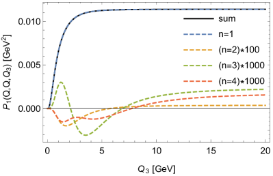
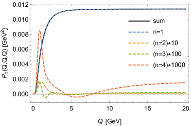
Figure 3: Plot of the contribution of the first four pion modes to $P_{1}(Q,Q,Q_{3})=-Q^{2}Q_{3}^{4}\Pi_{1}^{(\pi)}(Q,Q,Q_{3})$ for the HW1m model with $Q=200$ GeV in the left panel and $Q_{3}=Q$ in the right panel, showing that the contribution from the tower of pseudoscalars to the LSDC is suppressed like $1/Q_{3}^{2}$ up to (here invisible) logarithmic corrections.

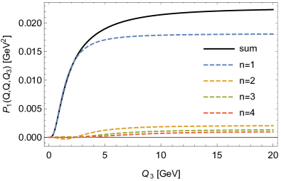
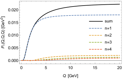
Figure 4: As in Fig. 3 but with quark masses increased by a factor of 25, illustrating the the build-up of a logarithmic enhancement by the summation of the infinite tower of massive pions.

IV.2.2 $Q_{1}^{2}=Q_{2}^{2}=Q_{3}^{2}\gg m_{\rho}^{2}$

In the symmetric limit $Q_{1}^{2}=Q_{2}^{2}=Q_{3}^{2}\gg m_{\rho}^{2}$, operator product expansion and LO pQCD imply that the longitudinal short distance constraint is 2/3 of value appearing in (45) Melnikov:2003xd ; Bijnens:2019ghy ,

$$\lim_{Q\to\infty}\lim_{Q\to\infty}Q^{4}\bar{\Pi}_{1}(Q,Q,Q)=-\frac{4}{9\pi^{2}}.$$ (59)

In this case, the same derivation as above leads to

$$\lim_{Q\to\infty}Q^{4}\bar{\Pi}_{1}^{\mathrm{AV}}(Q,Q,Q)$$

$$=-\frac{g_{5}^{2}}{2\pi^{4}}\int_{0}^{\infty}d\xi\int_{0}^{\infty}d\xi^{\prime}\frac{1}{2}\frac{d}{d\xi}[\xi K_{1}(\xi)]^{2}\frac{d}{d\xi^{\prime}}[\xi^{\prime}K_{1}^{\prime}(\xi^{\prime})]\frac{1}{2}[\mathrm{min}(\xi,\xi^{\prime})]^{2}$$

$$=-\frac{g_{5}^{2}}{(2\pi)^{2}\pi^{2}}\int_{0}^{\infty}d\xi\int_{0}^{\infty}d\xi^{\prime}[\xi K_{1}(\xi)]^{2}[\xi^{\prime}K_{1}^{\prime}(\xi^{\prime})]\xi\delta(\xi-\xi^{\prime})$$

$$=-\frac{g_{5}^{2}}{(2\pi)^{2}\pi^{2}}\int_{0}^{\infty}d\xi\,\xi[\xi K_{1}(\xi)]^{3}=-0.361\frac{g_{5}^{2}}{(2\pi)^{2}\pi^{2}},$$ (60)

which reproduces the correct power behavior, but for $g_{5}=2\pi$, as demanded by (14), the numerical value is only 81% of the result (59). Again, this result for the contribution of the infinite tower of axial vector mesons is the same for chiral and for massive HW models.

The asymptotic contribution of the pseudoscalar tower is still given by the expression (51), but the argument given thereafter does not apply in the symmetric limit. However, numerically we found no evidence of an enhancement of the asymptotic behavior due to the summation of the infinite tower of massive pions beyond what is seen in the asymmetric case, see Figs. 3 and 4.

V Numerical Results

In the following we compare the different HW models numerically, in particular with regard to the contribution of the infinite tower of massive pions to the hadronic light-by-light scattering amplitude and thereby to the anomalous magnetic moment of the muon.

In all models we have chosen $g_{5}=2\pi$, ensuring an exact fit of the asymptotic LO pQCD result (14), but in the later discussion we shall also consider relaxing this constraint to account for the fact that at any large but finite energy scale there is a nonnegligible reduction of TFFs of the order $\alpha_{s}/\pi$ that in AdS/QCD could perhaps be simply modelled by a small reduction of $g_{5}$. The low-energy parameters $f_{\pi}$ and $m_{\rho}$ are always fitted to their physical values, fixed to 92.4 MeV and 775 MeV, respectively, to be consistent with our previous work Leutgeb:2019gbz .

We consider two possibilities (HW1, HW3) for boundary conditions at $z=z_{0}$ [always given by (11)], and also alternatively the standard choice $M_{X}^{2}=-3$ and having $M_{X}^{2}$ as a tunable parameter. We thus employ four different HW models with nonvanishing light quark masses.

HW1m

is the direct extension of the chiral HW1 model employed in our previous studies Leutgeb:2019zpq ; Leutgeb:2019gbz . It coincides with model A of Erlich, Katz, Son and Stephanov Erlich:2005qh except that we have fitted to the mass of the neutral instead of the charged pions;

HW1m’

deviates from the standard choice $M_{X}^{2}=-3$ in order to attempt a better fit of the masses of the first excited pion and/or the lightest axial vector meson. It turns out that only the latter can be matched to the $a_{1}$ mass. The mass of the first excited pion is then also reduced compared to the pristine HW1 model, from around 1900 to 1600 MeV, but the target of 1300 MeV cannot be reached.

HW3m

uses the standard choice $M_{X}^{2}=-3$, but boundary conditions as proposed in Domenech:2010aq , which have the advantage of making a manual subtraction of infrared boundary contributions in the Chern-Simons action unnecessary;

HW3m’

uses additionally $M_{X}^{2}$ as a free parameter, which in this model achieves a fit of the mass of the first excited pion of 1300 MeV, as was the main motivation put forward by Domènech, Panico, and Wulzer in Ref. Domenech:2010aq for proposing this kind of model. Our HW3m’ slightly deviated from the parameters used in Ref. Domenech:2010aq because we fitted $f_{\pi}$, $m_{\rho}$, $m_{\pi^{0}}$, and $m_{\pi(1300)}$ instead of performing a least-squares fit over a larger set of low-energy parameters.

For the chiral limit, we only consider the HW1 model, where we update the results obtained for pions in Leutgeb:2019zpq and recapitulate the results for axial vector mesons in Leutgeb:2019gbz .

V.1 Masses

As Table 1 shows, in the chiral HW1 model the mass of the lightest axial-vector multiplet is above the physical masses PDG20 $M_{a_{1}(1260)}=1230(40)$ MeV and $M_{f_{1}(1285)}=1281.9(5)$ MeV, but below that of the $f_{1}^{\prime}$, $M_{f_{1}(1420)}=1426.3(9)$ MeV. While this prediction of the HW1 model is in the right ballpark, the mass of the first excited pion is 1899 MeV and thus significantly above $M_{\pi(1300)}=1300\pm 100$ MeV.

With nonzero light quark masses, the HW1m model has slightly reduced axial-vector meson mass and increased excited pion masses. In the HW1m’, where the $a_{1}$ mass can be matched, the lowest excited pion mass is reduced to about 1600 MeV.

With HW3 boundary conditions, there is additional chiral symmetry breaking and therefore a larger difference between the vector and axial vector meson masses, so that $m_{a_{1}}$ is now even above the mass of the physical $f_{1}^{\prime}$, but the excited pion mass is lowered substantially compared to the HW1m model, while still being too high. In the HW3m’ model, where the first excited pion can be brought down to 1300 MeV, the axial vector meson mass is then also lowered, but somewhat larger than in the HW1 models. Even in the HW3m’ model, where the pseudoscalar masses are the smallest, the second excited ($n=3$) pion has a mass higher than the next established pion state $\pi(1800)$ and instead close to the next (less established) state $\pi(2070)$; in the other models $m_{n=3}$ is far higher.

V.2 Decay constants

The results for the decay constant of the lowest excited pion in the massive HW models span the range (1.56…1.92) MeV, with the HW3m’ model, where the mass of $\pi(1300)$ can be fitted, yielding the largest value. These values are well below the existing experimental upper bound of 8.4 MeV Diehl:2001xe ; the result for the HW3m’ model is actually fully consistent with the value 2.20(46) MeV of Ref. Maltman:2001gc that was adopted in Ref. Colangelo:2019uex .

The holographic results for the decay constant of the lightest axial vector meson, defined in analogy to (13), read $F_{a_{1}}=(493\,\text{MeV})^{2}$ in the chiral HW1 model and $(426\ldots 506\,\text{MeV})^{2}$ for the different massive HW models. Note that in the literature frequently the mass of the axial vector meson is factored out Ecker:1988te ; *Ecker:1989yg. In Ref. Yang:2007zt a value of $F_{a_{1}}/m_{a_{1}}=168(7)$ MeV has been obtained from light-cone sum rules. With $F_{a_{1}}/m_{a_{1}}=177$ MeV for the chiral HW1 model and (148…195) MeV for the different massive HW models (see Table 1), the ballpark spanned by the holographic results is broadly consistent with that.

model	PS	$n=1$	$n=2$	$n=3$	AV	$n=1$	$n=2$	$n=3$	$n=4$	$n=5$
HW1 chiral	$m_{\pi_{n}}$[MeV]	$0\Rsh 135$	1899	2887	$m_{\mathrm{A}_{n}}$[MeV]	1375	2154	2995	3939	4917
$M_{X}^{2}=-3$	$f_{\pi_{n}}$ [MeV]	92.4*	0	0	$F_{\mathrm{A}_{n}}/m_{\mathrm{A}_{n}}$ [MeV]	177	204	263	311	351
	$F_{\pi_{n}\gamma\gamma}$[GeV-1]	0.274	-0.202	0.153	$A(0,0)$ [GeV-2]	-21.04	-2.93	0.294	-2.16	0.400
	$a_{\mu}^{\pi_{n}}\cdot 10^{11}$	65.2	0.7	0.1	$a_{\mu}^{\mathrm{A}_{n}}\cdot 10^{11}$	31.4	4.7	1.8	1.2	0.5
HW1m	$m_{\pi_{n}}$[MeV]	135*	1892	2882	$m_{\mathrm{A}_{n}}$[MeV]	1367	2141	2987	3934	4914
$M_{X}^{2}=-3$	$f_{\pi_{n}}$ [MeV]	92.4*	1.56	1.25	$F_{\mathrm{A}_{n}}/m_{\mathrm{A}_{n}}$ [MeV]	175	204	263	311	351
	$F_{\pi_{n}\gamma\gamma}$[GeV-1]	0.276	-0.203	0.154	$A(0,0)$ [GeV-2]	-21.00	-3.21	0.328	-2.16	0.376
	$a_{\mu}^{\pi_{n}}\cdot 10^{11}$	66.0	0.7	0.1	$a_{\mu}^{\mathrm{A}_{n}}\cdot 10^{11}$	31.4	4.9	1.8	1.2	0.5
HW1m’	$m_{\pi_{n}}$[MeV]	135*	1591	2564	$m_{\mathrm{A}_{n}}$[MeV]	1230*	1977	2901	3879	4873
$M_{X}^{2}=-3.837$	$f_{\pi_{n}}$ [MeV]	92.4*	1.59	0.950	$F_{\mathrm{A}_{n}}/m_{\mathrm{A}_{n}}$ [MeV]	148	208	266	312	351
	$F_{\pi_{n}\gamma\gamma}$[GeV-1]	0.277	-0.250	0.194	$A(0,0)$ [GeV-2]	-19.95	-7.29	0.678	-2.18	0.341
	$a_{\mu}^{\pi_{n}}\cdot 10^{11}$	64.3	1.5	0.3	$a_{\mu}^{\mathrm{A}_{n}}\cdot 10^{11}$	29.8	8.7	2.0	1.3	0.5
HW3m	$m_{\pi_{n}}$[MeV]	135*	1715	2513	$m_{\mathrm{A}_{n}}$[MeV]	1431	2421	3398	4387	5384
$M_{X}^{2}=-3$	$f_{\pi_{n}}$ [MeV]	92.4*	1.56	1.34	$F_{\mathrm{A}_{n}}/m_{\mathrm{A}_{n}}$ [MeV]	195	244	291	332	369
	$F_{\pi_{n}\gamma\gamma}$[GeV-1]	0.277	-0.196	0.0797	$A(0,0)$ [GeV-2]	-21.27	0.310	-2.09	-0.299	-0.514
	$a_{\mu}^{\pi_{n}}\cdot 10^{11}$	66.6	0.8	0.04	$a_{\mu}^{\mathrm{A}_{n}}\cdot 10^{11}$	32.7	3.4	1.7	0.7	0.4
HW3m’	$m_{\pi_{n}}$[MeV]	135*	1300*	2113	$m_{\mathrm{A}_{n}}$[MeV]	1380	2355	3345	4345	5350
$M_{X}^{2}=-3.841$	$f_{\pi_{n}}$ [MeV]	92.4*	1.92	1.29	$F_{\mathrm{A}_{n}}/m_{\mathrm{A}_{n}}$ [MeV]	186	242	291	332	369
	$F_{\pi_{n}\gamma\gamma}$[GeV-1]	0.278	-0.206	0.0474	$A(0,0)$ [GeV-2]	-21.29	-0.841	-1.76	-0.440	-0.476
	$a_{\mu}^{\pi_{n}}\cdot 10^{11}$	66.0	1.5	0.01	$a_{\mu}^{\mathrm{A}_{n}}\cdot 10^{11}$	33.2	4.1	1.8	0.8	0.4

Table 1: Numerical results for various HW models (in the chiral HW1 model with the pion mass raised manually ($\Rsh$) to 135 MeV in the evaluation of $a_{\mu}$). Fitted values are marked by $*$. The axial vector contributions correspond to a whole $U(N_{f}=3)$ multiplet, which in the present flavor-symmetric case is simply $a_{\mu}^{A_{n}}=a_{\mu}^{(a_{1}+f_{1}+f_{1}^{\prime})_{n}}=4a_{\mu}^{{a_{1}}_{n}}$.

V.3 Comparison of transition form factors

In Figs. 5 and 6 the single and double-virtual pion TFF following from the chiral and the massive HW models are compared with each other and with the results obtained in Hoferichter:2018kwz in the dispersive approach Colangelo:2015ama . The HW results all lie within the error band of the dispersive result, mostly above its central value, with only HW1m’ below.

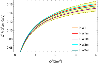
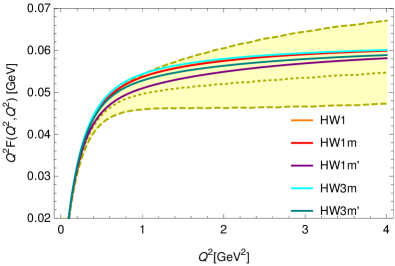
Figure 5: Single and double-virtual pion transition form factors in the various HW models together with the result of the data-driven dispersive approach of Ref. Hoferichter:2018kwz (yellow band for the estimated error with dotted dark-yellow points for the central result).

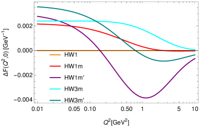
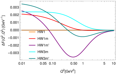
Figure 6: Deviations of the single and double-virtual pion transition form factors in the massive HW models from the chiral HW1 model.

Table 1 also lists the amplitude $F_{\pi_{n}\gamma\gamma}$ for pseudoscalar decays into two real photons. For the ground state pion there is only a tiny change when finite quark masses are introduced, across all massive HW models. For excited pions there is more variation; for the first excited pion the range of $|F_{\pi_{2}\gamma\gamma}|$ is (0.196…0.250) GeV^-1. In the HW3m’ model, where one can fit to $m_{2}=1300$ MeV, the value is 0.206 GeV^-1. At present, no direct measurements are available, but data on certain branching ratios permit to derive an estimate for an upper bound Colangelo:2019uex reading $|F_{\pi(1300)\gamma\gamma}|<0.0544(71)\text{Gev}^{-1}$. Evidently, the holographic results strongly overestimate the two-photon coupling of the first excited pion. This could be taken as a hint that it is better to choose a model where the masses of the lightest axial vector mesons can be fitted to experiment, namely the HW1m’ model, since the two-photon couplings of axial vector mesons play a more important role altogether. The holographic results obtained for the whole tower of excited pions could still be taken as a rough estimate of (perhaps an upper bound of) this contribution in real QCD. It is certainly also conceivable that the contributions of individual modes are overestimated while their combined contribution is closer to real QCD, where the mass spectrum of excited pions is denser than in the HW models.

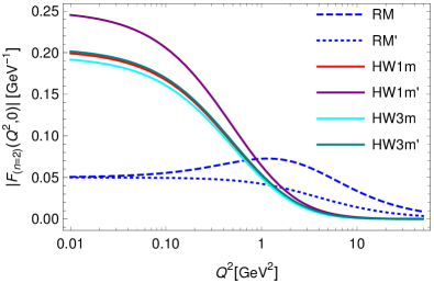
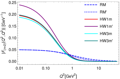
Figure 7: Single and double-virtual TFFs for the first excited pion in the various HW models. Also given are the corresponding quantities in the Regge model of Ref. Colangelo:2019lpu ; Colangelo:2019uex (RM) and its modification according to App. E therein (RM’).

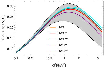
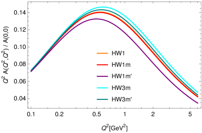
Figure 8: Single and double-virtual axial vector transition form factors, the former compared with the dipole fit of L3 data for $f_{1}(1285)$ of Ref. Achard:2001uu (grey band).

Table 1 also shows that the chiral HW1 model has almost identical results for $F_{\pi_{n}\gamma\gamma}$ as the HW1m model. As emphasized in Ref. Colangelo:2019uex , the vanishing of the decay constants of massive pions in the chiral limit does not preclude a coupling to photons. The former only means decoupling of the massive pions from the axial vector current and the axial anomaly. Thus massive pions contribute to the HLBL scattering amplitude also in the chiral HW1 model and therefore to the anomalous magnetic moment of the muon.

Fig. 7 displays the single and double-virtual TFFs for the first excited pion in the various HW models. Also shown are the corresponding quantities in the Regge model of Ref. Colangelo:2019lpu ; Colangelo:2019uex (RM) and its modification according to App. E therein (RM’). The Regge model TFFs satisfy the experimental upper bound $F_{\pi(1300)\gamma\gamma}$, but do not obey the single-virtual Brodsky-Lepage limit with the decay constants of excited pseudoscalars. The HW results have a much larger amplitude at vanishing virtualities, but decay faster. They have a zero and a sign change before approaching the asymptotic behavior (41). The TFFs of higher excited pions have more zeros and reduced asymptotic limits due to smaller decay constants.

In Fig. 8 the shape of the axial vector TFF $A(Q_{1}^{2},Q_{2}^{2})/A(0,0)$ is shown in the single-virtual and in the symmetric double-virtual cases. In the single-virtual case we also show the experimental result obtained in Achard:2001uu for the $f_{1}(1285)$ meson which is found to be remarkably compatible, in particular for the HW1m’ model, where the mass of the lightest axial vector meson can be fitted.

The normalization factor $A(0,0)$ is directly related to the so-called equivalent two-photon rate Schuler:1997yw ; Pascalutsa:2012pr . In Ref. Leutgeb:2019gbz we have compared with a combination of the experimental results obtained for the $f_{1}(1285)$ and $f_{1}(1420)$ meson. Since we are actually using flavor-symmetric models, one should account for SU(3) flavor breaking before matching $A(0,0)$, which leads to $|A(0,0)|_{f_{1}(1285)}^{\mathrm{exp.}}=16.6(1.5)\,\text{GeV}^{-2}$. In Refs. Roig:2019reh ; Masjuan:2020jsf the corresponding value for the lightest $a_{1}$ meson has been estimated as $|A(0,0)|^{\mathrm{exp}}_{a_{1}(1260)}=19.3(5.0)\,\text{GeV}^{-2}$. In the HW models we find the range $|A(0,0)|_{n=1}=(19.95\ldots 21.29)\,\text{GeV}^{-2}$ which is compatible with the latter, but above the value obtained for the $f_{1}(1285)$ meson.

V.4 HLBL contribution to $a_{\mu}$

In Table 1 we also give the holographic results for the contributions to $a_{\mu}$, the anomalous magnetic moment of the muon, from the first few states of the pion and axial vector meson towers; in Fig. 9 the results for the $\pi^{0}$ and $a_{1}$ sector are shown in form of a bar chart.

In the chiral HW1 model, the chiral TFFs for the pion have been combined with a pion propagator where the physical mass of $\pi^{0}$ has been inserted by hand. The result of $a_{\mu}^{\pi^{0}}=65.2\times 10^{-11}$ is remarkably close to that obtained in the massive HW models, which together span the range $a_{\mu}^{\pi^{0}}=(64.3\ldots 66.6)\times 10^{-11}$. The results of the massive HW1m are very close to those of the chiral HW1 model, also for the other contributions. Somewhat more variation is obtained in the other models, where either different boundary conditions or different values of $M_{X}^{2}$ are employed.

model${}^{1^{1^{1}}}$	$a_{\mu}^{\pi^{0}}$	$a_{\mu}^{\pi}$	$a_{\mu}^{\pi\cup a_{1}}$	$a_{\mu(L)}^{\pi^{*}\cup a_{1}}$	$a_{\mu(L)}^{\pi^{*}\cup a_{1}^{*}}$	$a_{\mu}^{\mathrm{P}^{*}}$	$a_{\mu}^{\mathrm{A}}[L+T]$	$a_{\mu}^{\mathrm{A}+\mathrm{P}^{*}}$
HW1	65.2	66.1	76.2	6.6	2.2	3.5	40.6[23.2+17.4]	44.0
HW1m	66.0	66.8	77.0	6.7	2.2	3.5	40.8[23.3+17.5]	44.3
HW1m’	64.3	66.1	77.0	8.1	3.7	7.2	43.3[25.0+18.3]	50.5
HW3m	66.6	67.4	77.4	6.5	1.9	3.4	39.9[22.7+17.2]	43.3
HW3m’	66.0	67.5	77.8	7.4	2.7	6.1	41.2[23.5+17.7]	47.3

Table 2: Partial sums of the contributions of pions and of axial vector mesons to $a_{\mu}$ in units of $10^{-11}$, where $a_{\mu(L)}$ denotes the longitudinal contribution only. Here $\pi$ and $a_{1}$ refer to the entire tower of pions and $a_{1}$ mesons; $\pi^{*}$ only to the heavy pions and $a_{1}^{*}$ only to excited axial vector mesons. A and P^∗ refer to a whole $U(N_{f}=3)$ multiplet of axial vector mesons and excited pseudoscalars, where the contributions from the former are split into longitudinal (L) and transverse (T) parts. In the present flavor-symmetric case $a_{\mu}^{\mathrm{A}}\equiv 4a_{\mu}^{a_{1}}$ and $a_{\mu}^{\mathrm{P}^{*}}\equiv 4a_{\mu}^{\pi^{*}}$.

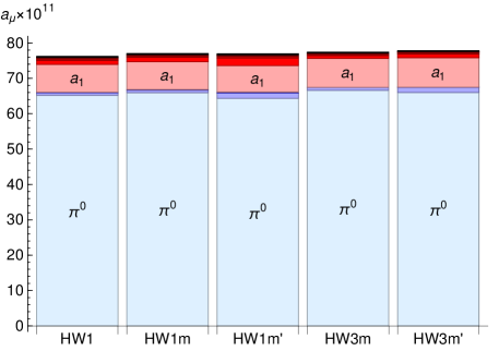
Figure 9: Bar chart of the individual contributions to $a_{\mu}^{\pi\cup a_{1}}$ in the various HW models, with excited modes given by increasingly darker colors, blue for the $\pi^{0}$’s, red for the $a_{1}$’s.

Table 2 shows the sums of the contributions in the different sectors, where we have made a numerical estimate of the limit value when the infinite tower of axial vector mesons is included as in Leutgeb:2019gbz ; in the case of the excited pions, the contributions of the higher modes fall off very quickly so that we have just summed the first few modes.

For the contributions of the excited pions we obtain the range $a_{\mu}^{\pi^{*}}=(0.8\ldots 1.8)\times 10^{-11}$ with the chiral model being at the lower end. Even though we have seen above that the HW models appear to severely overestimate the two-photon coupling $F_{\pi_{2}\gamma\gamma}$ when comparing with the upper limit Colangelo:2019uex $|F_{\pi(1300)\gamma\gamma}|$ given above, the holographic results are somewhat below the contributions from the first few excited states obtained in Colangelo:2019uex with large-$N_{c}$ Regge models. In Ref.Leutgeb:2019zpq also the contributions from the $\eta$ and $\eta^{\prime}$ pseudoscalars were estimated on the basis of the chiral HW1 model; we defer a precise evaluation of those in the massive HW models to future work where we plan to study the flavor-asymmetric case together with the contributions from the Witten-Veneziano mechanism for implementing the $U(1)_{A}$ anomaly. In the present flavor-symmetric setup, we would simply estimate the contribution of a whole $U(N_{f}=3)$ multiplet ($P^{*}$) as $a_{\mu}^{\mathrm{P}^{*}}\equiv 4a_{\mu}^{\pi^{*}}=(3.4\ldots 7.2)\times 10^{-11}$.

The much higher contributions from the infinite tower of axial vector mesons, which in the chiral HW1 model reads Leutgeb:2019gbz $a_{\mu}^{\mathrm{A}}=40.6\times 10^{-11}$, span the range $(39.3\ldots 43.3)\times 10^{-11}$ in the massive HW models, where the highest value is obtained in the HW1m’ model in which the physical mass of the $a_{1}$ meson can be fitted by using a nonstandard $M_{X}$ value. This model has also the largest contribution from the excited pseudoscalars, so that in combination $a_{\mu}^{\mathrm{A}+\mathrm{P}^{*}}=50.5\times 10^{-11}$ is reached; the lower end of the results for this quantity is provided by the HW3m model with $43.3\times 10^{-11}$, where the masses of axial vector mesons are in fact too high overall.

Generally we find that the contributions from excited axial vector mesons are more important than excited pions, corresponding to the fact that only the infinite tower of the former plays a role in satisfying the LSDCs (which is completely satisfied in the asymmetric Melnikov-Vainshtein case, and at the level of 81% in the symmetric case). Massive pions already contribute in the HW1 and HW3 models in the chiral limit; away from the chiral limit their importance is not increased, despite the different asymptotic behavior of their summed contribution in the HW1m and HW3m cases where one has a logarithmic enhancement of the TFFs. Correspondingly, the contributions of the axial vector tower are not reduced; in fact, they tend to be higher with nonzero quark masses.

V.5 Discussion

$\frac{g_{5}^{2}N_{c}}{12\pi^{2}}$	$R(A(0,0)_{n=1})$	$R(a_{\mu}^{P_{1},P})$	$R(a_{\mu}^{\mathrm{A}_{1}})$	$R(a_{\mu}^{\mathrm{A}})$
0.90	0.93	0.96	0.91	0.95
0.85	0.90	0.94	0.87	0.92

Table 3: Reduction factors $R$ in pseudoscalar and axial vector contributions to $a_{\mu}$ as estimated from the chiral HW model when the asymptotic LO pQCD constraints for TFFs are satisfied only at the levels of 90% or 85%. $P$ and $A$ refer to the whole tower of pseudoscalar and axial vector mesons, $P_{1}$ and $A_{1}$ to the ground-state modes.

Since we have seen above that the holographic results for the low-energy observables $F_{\pi_{2}\gamma\gamma}$ and $A_{1}(0,0)$, the latter determining the equivalent two-photon rate of the lightest axial vector meson, are larger than indicated by experiments, the corresponding holographic results may perhaps be viewed as upper limits. In the following we investigate whether this situation improves when one tries to accommodate corrections to the high-energy behavior. In fact, the holographic HW models we have considered here have no running coupling constant; the TFFs reach their asymptotic UV limits somewhat too quickly.

In order to derive more plausible extrapolations to real QCD, we have considered a reduction of the value $g_{5}^{2}$ by 10% and by 15%. This brings the asymptotic behavior of the TFFs down by amounts that are roughly consistent with perturbative corrections to the leading-order pQCD results at moderately high $Q^{2}$ values Melic:2002ij ; Bijnens:2021jqo . At the same time, the right-hand side of (14) is increased by a similar amount, which is consistent with the next-to-leading order terms in this expression Shifman:1978bx .

With 10% reduction, the HW model results for the pion TFF also get closer to the central result of the dispersive approach at all energies, while with 15% they are generally somewhat lower. In Table 3 we have listed the reduction factors resulting for $A_{1}(0,0)$ and various $a_{\mu}$ contributions in the chiral HW1 model which we assume to be a good approximation in general. Applying the stronger reduction factors to the minimum values of the results of the massive HW models, we obtain the range

$$a_{\mu}^{\pi^{0}} = (R(a_{\mu}^{P_{1}})_{0.85}\times 64.3\ldots 66.6)\times 10^{-11}$$ (61)

$$= (60.5\ldots 66.6)\times 10^{-11},$$

in remarkable agreement with recent evaluations using the data-driven dispersive approach Hoferichter:2018kwz , where $a_{\mu}^{\pi^{0}}=62.6^{+3.0}_{-2.5}\times 10^{-11}$, which has also been backed up by lattice QCD Gerardin:2019vio . Doing the same for excited pseudoscalars and axial vector mesons, we obtain the following ranges as our predictions for the contributions of excited pseudoscalars and axial vector mesons:

$$a_{\mu}^{\mathrm{P}^{*}}\equiv 4a_{\mu}^{\pi^{*}}=(3.2\ldots 7.2)\times 10^{-11},$$

$$a_{\mu(L)}^{\mathrm{A}}=(20.8\ldots 25.0)\times 10^{-11},$$

$$a_{\mu}^{\mathrm{A}}=(36.6\ldots 43.3)\times 10^{-11},$$

$$a_{\mu}^{\mathrm{A}+\mathrm{P}^{*}}=(39.8\ldots 50.5)\times 10^{-11}.$$ (62)

The latter result could be compared to the White Paper Aoyama:2020ynm values attributed to the axial sector and contributions related to the SDC, $a_{\mu}^{\mathrm{WP,axials}}=6(6)\times 10^{-11}$ and $a_{\mu}^{\mathrm{WP,SDC}}=15(10)\times 10^{-11}$, which with linearly added errors gives $21(16)\times 10^{-11}$, which is significantly smaller.

In Ref. Ludtke:2020moa , a model-independent estimate of the effects of the longitudinal short-distance constraints on the HLBL contribution to $a_{\mu}$ has been proposed with the result $\Delta a_{\mu}^{(3)}=2.6(1.5)\times 10^{-11}$ for the isovector sector. In Table 2 we have also listed the results for the longitudinal part of the contributions from the excited pions and the $a_{1}$ tower. Extending the range of the holographic results by the above reduction of the lower end, we obtain $a_{\mu(L)}^{\pi^{*}\cup a_{1}}=(6.0\ldots 8.1)\times 10^{-11}$ which is significantly higher. However, excluding the ground-state axial vector meson, whose mass is close to the matching scale used in Ludtke:2020moa and which (like any single excitation) does not contribute to the asymptotic value of the TFFs, we just have $a_{\mu(L)}^{\pi^{*}\cup a_{1}^{*}}=(1.7\ldots 3.7)\times 10^{-11}$, in perfect agreement with $\Delta a_{\mu}^{(3)}$ of Ref. Ludtke:2020moa . Including singlet and octet contributions, Ref. Ludtke:2020moa has estimated $\Delta a_{\mu}^{(0)+(3)+(8)}=9.1(5.0)\times 10^{-11}$, which is 3.5 times the $\Delta a_{\mu}^{(3)}$ result. In our flavor-symmetric models, we would have to multiply our results by a factor of 4, giving $(6.9\ldots 15.0)\times 10^{-11}$, which is still agreeing well. It would be interesting to revisit the additional study in Ref. Ludtke:2020moa where the HW2 results for the lightest axial vector meson were included and a result was found that exceeded the contributions of the remaining tower.

Another method to estimate the effects of the LSDC has been used in Colangelo:2019lpu ; Colangelo:2019uex , where a Regge model of excited pseudoscalars has been tuned to reproduce the LSDC. Although we have found in the holographic models that also away from the chiral limit it is the axial vector mesons that are alone responsible for the LSDC, the recently updated estimate obtained in Colangelo:2021nkr , $\Delta a_{\mu}^{\mathrm{LSDC}}=13(5)$, is fully consistent with our conclusions, as illustrated in Fig. 10.

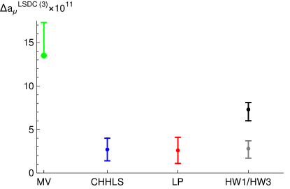
Figure 10: Isovector part of the longitudinal contributions beyond the pion pole. The original estimate of Melnikov-Vainshtein Melnikov:2003xd (MV) of $13.5\times 10^{-11}$ (green dot) translates to $17.5\times 10^{-11}$ with current input according to Colangelo:2019lpu ; Colangelo:2019uex . The estimate obtained by the latter, who have constructed a Regge model for excited pseudoscalars to reproduce the MV-SDC, is shown in blue and labelled CHHLS. The estimate of Lüdtke and Procura Ludtke:2020moa (LP) is plotted in red. The spread of results obtained in the HW1/HW3 models is shown in black; the gray version is without the contribution from the ground-state $a_{1}$ meson. (The center of the error bar is the center of the uncorrected results, and the errors are enlarged downwards according to the 85% reduction of $g_{5}^{2}$.)

The most important contribution missing in previous evaluations of the HLBL piece of $a_{\mu}$, if the holographic HW models are to be trusted, are those from the ground-state axial vector mesons. With the reduction of $g_{5}$, also the low energy end of the axial vector TFF gets modified appreciably, expanding our range of predictions to $|A(0,0)|_{n=1}=(17.3\ldots 21.3)\,\text{GeV}^{-2}$, which now has overlap with the experimental values quoted above in Sec. V.3. The lowest value (which also fits the experimental data best) is in fact obtained in the HW1m’ model, where the mass of $a_{1}(1260)$ can be fitted, yielding $a_{\mu}^{\mathrm{A}_{1}}=25.9\times 10^{-11}$. In this model, however, the $n=2$ axial vector TFF has a larger value than in the other models, and its contribution to $a_{\mu}$ is also fairly large, so that the second lightest axial vector multiplet alone contributes another $a_{\mu}^{\mathrm{A}_{2}}=7.5\times 10^{-11}$, despite having a mass much higher than that of established excited axial vector mesons. As we have already remarked, the total contribution of the axial vector tower is the largest of all HW models (see Table 2). With maximal reduction of $g_{5}^{2}$ it still yields $a_{\mu}^{\mathrm{A}}=40\times 10^{-11}$, coinciding with the central value of the range given in (V.5).

All in all, the holographic HW models that we have considered here point to $\gtrsim 20\times 10^{-11}$ of extra contributions in the HLBL part of $a_{\mu}$ compared to the axial-vector and SDC pieces in the White Paper value Aoyama:2020ynm of $a_{\mu}^{\mathrm{HLBL,WP}}=92(18)\times 10^{-11}$, chiefly due to the axial vector meson contributions. Such sizable upwards corrections are in fact compatible with the recent complete lattice calculation Chao:2021tvp with comparable errors, which obtained $a_{\mu}^{\mathrm{HLBL,lattice}}=106.8(14.7)\times 10^{-11}$.

VI Conclusion

In this paper we have studied various AdS/QCD models with a hard wall and with a bifundamental scalar which permits to introduce finite quark masses and thus to extend our previous work on hadronic light-by-light contributions in holographic QCD away from the chiral limit. In the latter it was shown in Ref. Leutgeb:2019gbz ; Cappiello:2019hwh that summation of the contributions of the infinite tower of axial vector mesons changes the asymptotic behavior of the HLBL scattering amplitude of individual contributions precisely such that the Melnikov-Vainshtein LSDC is satisfied. By contrast, in Colangelo:2019lpu ; Colangelo:2019uex a Regge model of excited pseudoscalars has been constructed to achieve the same. Turning on finite quark masses, we found that in the holographic models the infinite tower of excited pseudoscalars, which is already present in the chiral limit and in fact has nonvanishing two-photon couplings despite vanishing decay constants, couples to the axial anomaly and then can lead to a certain enhancement of their contribution to the asymptotic HLBL amplitude, but never enough to contribute to the leading terms of the LSDCs. With the standard choice of the holographic mass of the bifundamental scalar, which determines the scaling dimension of quark masses and chiral condensates, this enhancement is merely logarithmic; generalizations are possible, where also power-law enhancements arise, but still below what is relevant for LSDCs at leading order.

We have also considered the numerical consequences of introducing finite quark masses on the results obtained previously in the chiral limit, for simplicity only in the flavor-symmetric limit so that the $\pi^{0}$ and the $a_{1}$ sector can be covered, leaving the $N_{f}=2+1$ case and also the consideration of the Witten-Veneziano mechanism for the U(1)_A anomaly to future work. Doing so we have explored the two sets of boundary conditions that are possible in hard-wall models, and we have also considered the generalization of modified scaling dimensions of quark masses and chiral condensates proposed in Domenech:2010aq , which permits to fit either the mass of the first excited pion or the mass of the lowest axial vector meson.

As displayed in Fig. 9, the massive HW models lead only to small (positive) changes in the contributions to $a_{\mu}$ from the $\pi^{0}$ and $a^{0}$ towers compared to the chiral HW1 model, when in the latter the physical pion mass is inserted manually in the pion propagator. Compared to experimental data, the two-photon couplings of the lowest axial vector meson, which is responsible for the second-largest contribution besides the ground state pion, is somewhat too large, but it becomes consistent with experimental constraints when the five-dimensional coupling is adjusted such that the LO pQCD values of TFFs is reduced by amounts corresponding to typical $\alpha_{s}$ corrections at moderately large energies. However, also after such adjustments, the contributions from the axial vector and excited pseudoscalar mesons ($\gtrsim 40\times 10^{-11}$) are significantly larger than in the model calculations that have been used to assess their role and also the effect of SDCs in the White Paper Aoyama:2020ynm , where $a_{\mu}^{\mathrm{axials+SDC}}=21(16)\times 10^{-11}$.

Appendix A Chiral limit and GOR relation

In the following we give some details on the chiral limit $M_{q}\to 0$ of the massive HW models, including the generalization where $M_{X}^{2}$ is allowed to deviate from the standard choice $M_{X}^{2}=-3$. The connection to the chiral HW models with strictly $M_{q}=0$ is somewhat subtle, because the weight function $z/\beta(z)$ in the differential equation (22) for $y=\partial_{z}\phi/z$ is (more) singular at $\zeta\equiv z/z_{0}=0$ when $M_{q}=0$,

$$\frac{z}{\beta(z)}\sim\left\{\begin{array}[]{ll}\frac{z_{0}}{g_{5}^{2}M_{q}^{2}}\zeta^{-1+2\alpha}&\mbox{for}\;\zeta\to 0,\,M_{q}\not=0\\ \frac{1}{g_{5}^{2}\Sigma^{2}z_{0}^{3}}\zeta^{-1-2\alpha}&\mbox{for}\;\zeta\to 0,\,M_{q}=0\end{array}\right.$$ (63)

where $\alpha=\sqrt{4+M_{X}^{2}}\in(0,2)$, with $\alpha=1$ for the standard choice $M_{X}^{2}=-3$.

The asymptotic behavior of the profile function $y_{S}(q,z)$ near the boundary $\zeta=0$ reads

$$y_{S}(q,z)\sim\left\{\begin{array}[]{ll}\frac{g_{5}^{2}M_{q}^{2}}{2-2\alpha}\zeta^{2-2\alpha}+a_{1}+a_{2}\zeta^{4-2\alpha}+\ldots&\mbox{for}\;\alpha>1\\ g_{5}^{2}M_{q}^{2}\ln\zeta+a_{1}+a_{2}\zeta^{2}\ln\zeta+\ldots&\mbox{for}\;\alpha=1\\ a_{0}+\frac{g_{5}^{2}M_{q}^{2}}{2-2\alpha}\zeta^{2-2\alpha}+a_{2}\zeta^{2}+\ldots&\mbox{for}\;\alpha<1\end{array}\right.$$ (64)

and that of normalizable modes is given by

$$y_{n}=-g_{5}f_{\pi_{n}}+\left\{\begin{array}[]{ll}c_{1}\zeta^{4-2\alpha}+\ldots&\mbox{for}\;\alpha>1\\ c_{1}\zeta^{2}+\ldots&\mbox{for}\;\alpha\leq 1\end{array}\right..$$ (65)

The mode functions $\phi_{n}$ and $\pi_{n}$ vanish at the ultraviolet boundary according to

$$\phi_{n}=-g_{5}f_{\pi_{n}}z^{2}/2+\ldots,\quad\pi_{n}=-\frac{m_{n}^{2}f_{\pi_{n}}z_{0}^{2-2\alpha}}{2\alpha g_{5}M_{q}^{2}}z^{2\alpha}+\ldots.$$ (66)

When $M_{q}\ll\Sigma z_{0}^{2}$, the weight function $z/\beta(z)$ is concentrated at small $z$, where its would-be divergence is cut off by $M_{q}$. In this limit, one can approximate the normalization condition (27) by replacing $y_{n}^{2}$ by its boundary value $g_{5}^{2}f_{\pi_{n}}^{2}$ and the upper limit of the integral by infinity, yielding

$$g_{5}^{2}f_{\pi_{n}}^{2}m_{n}^{2}\int_{0}^{\infty}dz\frac{z}{\beta(z)}=1,$$ (67)

where

$$g_{5}^{2}\int_{0}^{\infty}dz\frac{z}{\beta(z)}=z_{0}^{4}\int_{0}^{\infty}d\zeta\frac{\zeta^{3}}{(z_{0}M_{q}\,\zeta^{\Delta^{-}}+z_{0}^{3}\Sigma\,\zeta^{\Delta^{+}})^{2}}$$

$$=z_{0}^{4}\int_{0}^{\infty}d\zeta\frac{\zeta^{2\alpha-1}}{(z_{0}M_{q}+z_{0}^{3}\Sigma\,\zeta^{2\alpha})^{2}}=\frac{1}{2\alpha M_{q}\Sigma}.$$ (68)

For sufficiently small $M_{q}$ we thus obtain

$$f_{\pi_{n}}^{2}m_{n}^{2}\approx 2\alpha M_{q}\Sigma.$$ (69)

For massive pions, i.e., for $n>1$, where $m_{n}$ approaches a nonzero value in the chiral limit, this implies that $f_{\pi_{n}}\to 0$, so they decouple, while the lightest pion with $f_{\pi_{1}}=f_{\pi}$ gives rise to the Gell-Mann–Oakes–Renner relation $f_{\pi}^{2}m_{\pi}^{2}=2M_{q}\Sigma_{q}$ for $\alpha=1$, while for $\alpha\not=1$ one should perhaps rescale $M_{q}$ and $\Sigma$ before interpreting them as quark mass and condensate. (The scaling factor mentioned in footnote 2 drops out here.)

While $y_{1}$ always satisfies the boundary condition $\frac{z}{\beta}\partial_{z}y_{1}=0$ at $z=\epsilon$ with $z/\beta\sim z^{-1+2\alpha}$ as $M_{q}\to 0$, it does not satisfy such a boundary condition with $\beta(z)|_{M_{q}=0}$. From the point of view of the strictly chiral HW model, $y_{1}$ corresponds to a solution with the different boundary conditions that pertain to the one of profile functions $y_{S}$ (up to an overall factor). Nevertheless, it can still be normalized by (27), since with the help of the equations of motion the divergent integral times the vanishing mass can be recast as

$$m_{1}^{2}\int_{\epsilon}^{z_{0}}dz\frac{z}{\beta(z)}y_{1}^{2}=\int_{\epsilon}^{z_{0}}dz\,y_{1}\left[z-\partial_{z}\frac{z}{\beta(z)}\partial_{z}\right]y_{1}.$$ (70)

The holographic wave function of the massless pion can be given in closed form as the appropriate linear combination of the two Bessel functions

$$z^{1+\alpha}I_{\pm\frac{1+\alpha}{2+\alpha}}\left(\frac{g_{5}\Sigma z_{0}^{1-\alpha}}{2+\alpha}z^{2+\alpha}\right).$$ (71)

In the special case of the chiral HW1 model with standard $M_{X}^{2}=-3$ and thus $\alpha=1$ the result reads Grigoryan:2007wn

$$y_{1}=Nz^{2}\left(-I_{-\frac{2}{3}}(\eta z^{3})+\frac{I_{-\frac{2}{3}}(\eta z_{0}^{3})}{I_{\frac{2}{3}}(\eta z_{0}^{3})}I_{\frac{2}{3}}(\eta z^{3})\right),$$ (72)

with $\eta=g_{5}\Sigma/3$ and $N^{2}=g_{5}^{2}\Sigma^{2}\Gamma(\frac{1}{3})\Gamma(\frac{2}{3}){I_{\frac{2}{3}}(\eta z_{0}^{3})}/{I_{-\frac{2}{3}}(\eta z_{0}^{3})}.$

Appendix B Effects of reducing $g_{5}^{2}$

The following table shows the changes brought about by a reduction of $g_{5}^{2}$ by 10% (HW1-) and by 15% (HW1–) in the chiral HW1 model.

model	PS	$n=1$	$n=2$	$n=3$	AV	$n=1$	$n=2$	$n=3$	$n=4$	$n=5$
HW1- chiral	$m_{\pi_{n}}$[MeV]	$0\Rsh 135$	1849	2847	$m_{\mathrm{A}_{n}}$[MeV]	1295	2065	2944	3906	4893
$M_{X}^{2}=-3$	$f_{\pi_{n}}$ [MeV]	92.4*	0	0	$F_{\mathrm{A}_{n}}/m_{\mathrm{A}_{n}}$ [MeV]	166	205	264	311	350
	$F_{\pi_{n}\gamma\gamma}$[GeV-1]	0.274	-0.209	0.161	$A(0,0)$ [GeV-2]	-19.65	-4.49	0.390	-2.06	0.353
	$a_{\mu}^{\pi_{n}}\cdot 10^{11}$	62.7	0.8	0.1	$a_{\mu}^{\mathrm{A}_{n}}\cdot 10^{11}$	28.7	5.6	1.7	1.1	0.4
HW1– chiral	$m_{\pi_{n}}$[MeV]	$0\Rsh 135$	1827	2830	$m_{\mathrm{A}_{n}}$[MeV]	1255	2027	2923	3892	4882
$M_{X}^{2}=-3$	$f_{\pi_{n}}$ [MeV]	92.4*	0	0	$F_{\mathrm{A}_{n}}/m_{\mathrm{A}_{n}}$ [MeV]	161	206	265	311	351
	$F_{\pi_{n}\gamma\gamma}$[GeV-1]	0.274	-0.213	0.166	$A(0,0)$ [GeV-2]	-18.90	-5.13	0.406	-2.00	0.332
	$a_{\mu}^{\pi_{n}}\cdot 10^{11}$	61.4	0.8	0.2	$a_{\mu}^{\mathrm{A}_{n}}\cdot 10^{11}$	27.3	5.9	1.7	1.1	0.4

Table 4: HW1 chiral models with reduced UV asymptotics. HW1- and HW1– have $g^{2}N_{c}/12\pi^{2}=0.90$ and 0.85, respectively.

References

- (1) Muon g-2 Collaboration, B. Abi et al., Measurement of the Positive Muon Anomalous Magnetic Moment to 0.46 ppm, Phys. Rev. Lett. 126 (2021), no. 14 141801, [arXiv:2104.03281].
- (2) Muon g-2 Collaboration, G. W. Bennett et al., Final Report of the Muon E821 Anomalous Magnetic Moment Measurement at BNL, Phys. Rev. D 73 (2006) 072003, [hep-ex/0602035].
- (3) F. Jegerlehner, The Anomalous Magnetic Moment of the Muon, Second Edition, Springer Tracts Mod. Phys. 274 (2017) pp.1–693.
- (4) T. Aoyama et al., The anomalous magnetic moment of the muon in the Standard Model, Phys. Rept. 887 (2020) 1–166, [arXiv:2006.04822].
- (5) T. Aoyama, M. Hayakawa, T. Kinoshita, and M. Nio, Complete Tenth-Order QED Contribution to the Muon g-2, Phys. Rev. Lett. 109 (2012) 111808, [arXiv:1205.5370].
- (6) T. Aoyama, T. Kinoshita, and M. Nio, Revised and Improved Value of the QED Tenth-Order Electron Anomalous Magnetic Moment, Phys. Rev. D97 (2018) 036001, [arXiv:1712.06060].
- (7) T. Aoyama, T. Kinoshita, and M. Nio, Theory of the Anomalous Magnetic Moment of the Electron, Atoms 7 (2019), no. 1 28.
- (8) A. Czarnecki, W. J. Marciano, and A. Vainshtein, Refinements in electroweak contributions to the muon anomalous magnetic moment, Phys. Rev. D67 (2003) 073006, [hep-ph/0212229]. [Erratum: Phys. Rev.D73,119901(2006)].
- (9) C. Gnendiger, D. Stöckinger, and H. Stöckinger-Kim, The electroweak contributions to after the Higgs boson mass measurement, Phys. Rev. D88 (2013) 053005, [arXiv:1306.5546].
- (10) K. Melnikov and A. Vainshtein, Hadronic light-by-light scattering contribution to the muon anomalous magnetic moment revisited, Phys. Rev. D70 (2004) 113006, [hep-ph/0312226].
- (11) J. Prades, E. de Rafael, and A. Vainshtein, The Hadronic Light-by-Light Scattering Contribution to the Muon and Electron Anomalous Magnetic Moments, Adv. Ser. Direct. High Energy Phys. 20 (2009) 303–317, [arXiv:0901.0306].
- (12) A. Kurz, T. Liu, P. Marquard, and M. Steinhauser, Hadronic contribution to the muon anomalous magnetic moment to next-to-next-to-leading order, Phys. Lett. B734 (2014) 144–147, [arXiv:1403.6400].
- (13) G. Colangelo, M. Hoferichter, A. Nyffeler, M. Passera, and P. Stoffer, Remarks on higher-order hadronic corrections to the muon , Phys. Lett. B735 (2014) 90–91, [arXiv:1403.7512].
- (14) V. Pauk and M. Vanderhaeghen, Single meson contributions to the muon’s anomalous magnetic moment, Eur. Phys. J. C74 (2014) 3008, [arXiv:1401.0832].
- (15) M. Davier, A. Hoecker, B. Malaescu, and Z. Zhang, Reevaluation of the hadronic vacuum polarisation contributions to the Standard Model predictions of the muon and using newest hadronic cross-section data, Eur. Phys. J. C77 (2017), no. 12 827, [arXiv:1706.09436].
- (16) P. Masjuan and P. Sanchez-Puertas, Pseudoscalar-pole contribution to the : a rational approach, Phys. Rev. D95 (2017) 054026, [arXiv:1701.05829].
- (17) G. Colangelo, M. Hoferichter, M. Procura, and P. Stoffer, Dispersion relation for hadronic light-by-light scattering: two-pion contributions, JHEP 04 (2017) 161, [arXiv:1702.07347].
- (18) A. Keshavarzi, D. Nomura, and T. Teubner, Muon and : a new data-based analysis, Phys. Rev. D97 (2018) 114025, [arXiv:1802.02995].
- (19) G. Colangelo, M. Hoferichter, and P. Stoffer, Two-pion contribution to hadronic vacuum polarization, JHEP 02 (2019) 006, [arXiv:1810.00007].
- (20) M. Hoferichter, B.-L. Hoid, and B. Kubis, Three-pion contribution to hadronic vacuum polarization, JHEP 08 (2019) 137, [arXiv:1907.01556].
- (21) M. Davier, A. Hoecker, B. Malaescu, and Z. Zhang, A new evaluation of the hadronic vacuum polarisation contributions to the muon anomalous magnetic moment and to , Eur. Phys. J. C 80 (2020) 241, [arXiv:1908.00921].
- (22) A. Keshavarzi, D. Nomura, and T. Teubner, of charged leptons, , and the hyperfine splitting of muonium, Phys. Rev. D 101 (2020) 014029, [arXiv:1911.00367].
- (23) M. Hoferichter, B.-L. Hoid, B. Kubis, S. Leupold, and S. P. Schneider, Pion-pole contribution to hadronic light-by-light scattering in the anomalous magnetic moment of the muon, Phys. Rev. Lett. 121 (2018), no. 11 112002, [arXiv:1805.01471].
- (24) M. Hoferichter, B.-L. Hoid, B. Kubis, S. Leupold, and S. P. Schneider, Dispersion relation for hadronic light-by-light scattering: pion pole, JHEP 10 (2018) 141, [arXiv:1808.04823].
- (25) A. Gérardin, H. B. Meyer, and A. Nyffeler, Lattice calculation of the pion transition form factor with Wilson quarks, Phys. Rev. D 100 (2019), no. 3 034520, [arXiv:1903.09471].
- (26) J. Bijnens, N. Hermansson-Truedsson, and A. Rodríguez-Sánchez, Short-distance constraints for the HLbL contribution to the muon anomalous magnetic moment, Phys. Lett. B 798 (2019) 134994, [arXiv:1908.03331].
- (27) G. Colangelo, F. Hagelstein, M. Hoferichter, L. Laub, and P. Stoffer, Short-distance constraints on hadronic light-by-light scattering in the anomalous magnetic moment of the muon, Phys. Rev. D 101 (2020) 051501, [arXiv:1910.11881].
- (28) G. Colangelo, F. Hagelstein, M. Hoferichter, L. Laub, and P. Stoffer, Longitudinal short-distance constraints for the hadronic light-by-light contribution to with large- Regge models, JHEP 03 (2020) 101, [arXiv:1910.13432].
- (29) I. Danilkin, C. F. Redmer, and M. Vanderhaeghen, The hadronic light-by-light contribution to the muon’s anomalous magnetic moment, Prog. Part. Nucl. Phys. 107 (2019) 20–68, [arXiv:1901.10346].
- (30) T. Blum, N. Christ, M. Hayakawa, T. Izubuchi, L. Jin, C. Jung, and C. Lehner, Hadronic Light-by-Light Scattering Contribution to the Muon Anomalous Magnetic Moment from Lattice QCD, Phys. Rev. Lett. 124 (2020) 132002, [arXiv:1911.08123].
- (31) E.-H. Chao, R. J. Hudspith, A. Gérardin, J. R. Green, H. B. Meyer, and K. Ottnad, Hadronic light-by-light contribution to from lattice QCD: a complete calculation, Eur. Phys. J. C 81 (2021), no. 7 651, [arXiv:2104.02632].
- (32) S. Borsanyi et al., Leading hadronic contribution to the muon magnetic moment from lattice QCD, Nature 593 (2021) 51–55, [arXiv:2002.12347].
- (33) A. Crivellin, M. Hoferichter, C. A. Manzari, and M. Montull, Hadronic Vacuum Polarization: versus Global Electroweak Fits, Phys. Rev. Lett. 125 (2020), no. 9 091801, [arXiv:2003.04886].
- (34) A. Keshavarzi, W. J. Marciano, M. Passera, and A. Sirlin, Muon and connection, Phys. Rev. D 102 (2020), no. 3 033002, [arXiv:2006.12666].
- (35) G. Colangelo, M. Hoferichter, and P. Stoffer, Constraints on the two-pion contribution to hadronic vacuum polarization, Phys. Lett. B 814 (2021) 136073, [arXiv:2010.07943].
- (36) M. Abe et al., A New Approach for Measuring the Muon Anomalous Magnetic Moment and Electric Dipole Moment, PTEP 2019 (2019) 053C02, [arXiv:1901.03047].
- (37) J. Leutgeb and A. Rebhan, Axial vector transition form factors in holographic QCD and their contribution to the anomalous magnetic moment of the muon, Phys. Rev. D 101 (2020) 114015, [arXiv:1912.01596].
- (38) L. Cappiello, O. Catà, G. D’Ambrosio, D. Greynat, and A. Iyer, Axial-vector and pseudoscalar mesons in the hadronic light-by-light contribution to the muon , Phys. Rev. D 102 (2020) 016009, [arXiv:1912.02779].
- (39) M. Knecht, On some short-distance properties of the fourth-rank hadronic vacuum polarization tensor and the anomalous magnetic moment of the muon, JHEP 08 (2020) 056, [arXiv:2005.09929].
- (40) P. Masjuan, P. Roig, and P. Sanchez-Puertas, The interplay of transverse degrees of freedom and axial-vector mesons with short-distance constraints in g-2, arXiv:2005.11761.
- (41) J. Erlich, E. Katz, D. T. Son, and M. A. Stephanov, QCD and a holographic model of hadrons, Phys. Rev. Lett. 95 (2005) 261602, [hep-ph/0501128].
- (42) L. Da Rold and A. Pomarol, Chiral symmetry breaking from five-dimensional spaces, Nucl. Phys. B721 (2005) 79–97, [hep-ph/0501218].
- (43) L. Da Rold and A. Pomarol, The Scalar and pseudoscalar sector in a five-dimensional approach to chiral symmetry breaking, JHEP 01 (2006) 157, [hep-ph/0510268].
- (44) L. Cappiello, O. Cata, and G. D’Ambrosio, The hadronic light by light contribution to the with holographic models of QCD, Phys. Rev. D83 (2011) 093006, [arXiv:1009.1161].
- (45) J. Leutgeb, J. Mager, and A. Rebhan, Pseudoscalar transition form factors and the hadronic light-by-light contribution to the anomalous magnetic moment of the muon from holographic QCD, Phys. Rev. D100 (2019) 094038, [arXiv:1906.11795]. Erratum to appear in Phys. Rev. D.
- (46) L3 Collaboration, P. Achard et al., formation in two-photon collisions at LEP, Phys. Lett. B526 (2002) 269–277, [hep-ex/0110073].
- (47) K. Ghoroku, N. Maru, M. Tachibana, and M. Yahiro, Holographic model for hadrons in deformed AdS5 background, Phys. Lett. B 633 (2006) 602–606, [hep-ph/0510334].
- (48) A. Karch, E. Katz, D. T. Son, and M. A. Stephanov, Linear confinement and AdS/QCD, Phys. Rev. D74 (2006) 015005, [hep-ph/0602229].
- (49) U. Gürsoy and E. Kiritsis, Exploring improved holographic theories for QCD: Part I, JHEP 02 (2008) 032, [arXiv:0707.1324].
- (50) U. Gürsoy, E. Kiritsis, and F. Nitti, Exploring improved holographic theories for QCD: Part II, JHEP 02 (2008) 019, [arXiv:0707.1349].
- (51) J. Lüdtke and M. Procura, Effects of longitudinal short-distance constraints on the hadronic light-by-light contribution to the muon , Eur. Phys. J. C 80 (2020), no. 12 1108, [arXiv:2006.00007].
- (52) G. Colangelo, F. Hagelstein, M. Hoferichter, L. Laub, and P. Stoffer, Short-distance constraints for the longitudinal component of the hadronic light-by-light amplitude: an update, Eur. Phys. J. C 81 (2021), no. 8 702, [arXiv:2106.13222].
- (53) J. Hirn and V. Sanz, Interpolating between low and high energy QCD via a 5-D Yang-Mills model, JHEP 12 (2005) 030, [hep-ph/0507049].
- (54) T. Sakai and S. Sugimoto, Low energy hadron physics in holographic QCD, Prog.Theor.Phys. 113 (2005) 843–882, [hep-th/0412141].
- (55) T. Sakai and S. Sugimoto, More on a holographic dual of QCD, Prog.Theor.Phys. 114 (2005) 1083–1118, [hep-th/0507073].
- (56) O. Domènech, G. Panico, and A. Wulzer, Massive Pions, Anomalies and Baryons in Holographic QCD, Nucl. Phys. A 853 (2011) 97–123, [arXiv:1009.0711].
- (57) H. R. Grigoryan and A. V. Radyushkin, Pion form-factor in chiral limit of hard-wall AdS/QCD model, Phys. Rev. D76 (2007) 115007, [arXiv:0709.0500].
- (58) Z. Abidin and C. E. Carlson, Strange hadrons and kaon-to-pion transition form factors from holography, Phys. Rev. D 80 (2009) 115010, [arXiv:0908.2452].
- (59) A. Cherman, T. D. Cohen, and E. S. Werbos, The Chiral condensate in holographic models of QCD, Phys. Rev. C 79 (2009) 045203, [arXiv:0804.1096].
- (60) A. Gorsky and A. Krikun, Magnetic susceptibility of the quark condensate via holography, Phys. Rev. D79 (2009) 086015, [arXiv:0902.1832].
- (61) H. J. Kwee and R. F. Lebed, Pion form-factors in holographic QCD, JHEP 01 (2008) 027, [arXiv:0708.4054].
- (62) D. T. Son and N. Yamamoto, Holography and Anomaly Matching for Resonances, arXiv:1010.0718.
- (63) H. R. Grigoryan and A. V. Radyushkin, Anomalous Form Factor of the Neutral Pion in Extended AdS/QCD Model with Chern-Simons Term, Phys. Rev. D77 (2008) 115024, [arXiv:0803.1143].
- (64) H. R. Grigoryan and A. V. Radyushkin, Pion in the Holographic Model with 5D Yang-Mills Fields, Phys. Rev. D78 (2008) 115008, [arXiv:0808.1243].
- (65) D. K. Hong and D. Kim, Pseudo scalar contributions to light-by-light correction of muon in AdS/QCD, Phys. Lett. B680 (2009) 480–484, [arXiv:0904.4042].
- (66) G. P. Lepage and S. J. Brodsky, Exclusive Processes in Quantum Chromodynamics: Evolution Equations for Hadronic Wave Functions and the Form-Factors of Mesons, Phys. Lett. 87B (1979) 359–365.
- (67) G. P. Lepage and S. J. Brodsky, Exclusive Processes in Perturbative Quantum Chromodynamics, Phys. Rev. D22 (1980) 2157.
- (68) S. J. Brodsky and G. P. Lepage, Large-Angle Two-Photon Exclusive Channels in Quantum Chromodynamics, Phys. Rev. D24 (1981) 1808.
- (69) A. V. Efremov and A. V. Radyushkin, Factorization and Asymptotical Behavior of Pion Form-Factor in QCD, Phys. Lett. 94B (1980) 245–250.
- (70) M. Hoferichter and P. Stoffer, Asymptotic behavior of meson transition form factors, JHEP 05 (2020) 159, [arXiv:2004.06127].
- (71) V. A. Novikov, M. A. Shifman, A. I. Vainshtein, M. B. Voloshin, and V. I. Zakharov, Use and Misuse of QCD Sum Rules, Factorization and Related Topics, Nucl. Phys. B 237 (1984) 525–552.
- (72) L. D. Landau, On the angular momentum of a system of two photons, Dokl. Akad. Nauk Ser. Fiz. 60 (1948) 207–209.
- (73) C.-N. Yang, Selection Rules for the Dematerialization of a Particle Into Two Photons, Phys. Rev. 77 (1950) 242–245.
- (74) V. Pascalutsa, V. Pauk, and M. Vanderhaeghen, Light-by-light scattering sum rules constraining meson transition form factors, Phys. Rev. D85 (2012) 116001, [arXiv:1204.0740].
- (75) P. Roig and P. Sanchez-Puertas, Axial-vector exchange contribution to the hadronic light-by-light piece of the muon anomalous magnetic moment, Phys. Rev. D 101 (2020) 074019, [arXiv:1910.02881].
- (76) M. Zanke, M. Hoferichter, and B. Kubis, On the transition form factors of the axial-vector resonance and its decay into , JHEP 07 (2021) 106, [arXiv:2103.09829].
- (77) G. Colangelo, M. Hoferichter, M. Procura, and P. Stoffer, Dispersion relation for hadronic light-by-light scattering: theoretical foundations, JHEP 09 (2015) 074, [arXiv:1506.01386].
- (78) A. Vainshtein, Perturbative and nonperturbative renormalization of anomalous quark triangles, Phys. Lett. B569 (2003) 187–193, [hep-ph/0212231].
- (79) P. A. Zyla et al., Review of Particle Physics, Prog. Theor. Exp. Phys. 2020 (2020) 083C01. 2021 updates available on-line.
- (80) M. Diehl and G. Hiller, New ways to explore factorization in b decays, JHEP 06 (2001) 067, [hep-ph/0105194].
- (81) K. Maltman and J. Kambor, Decay constants, light quark masses and quark mass bounds from light quark pseudoscalar sum rules, Phys. Rev. D 65 (2002) 074013, [hep-ph/0108227].
- (82) V. Elias, A. Fariborz, M. A. Samuel, F. Shi, and T. G. Steele, Beyond the narrow resonance approximation: Decay constant and width of the first pion excitation state, Phys. Lett. B 412 (1997) 131–136, [hep-ph/9706472].
- (83) A. L. Kataev, N. V. Krasnikov, and A. A. Pivovarov, The Use of the Finite Energetic Sum Rules for the Calculation of the Light Quark Masses, Phys. Lett. B 123 (1983) 93.
- (84) G. Ecker, J. Gasser, A. Pich, and E. de Rafael, The Role of Resonances in Chiral Perturbation Theory, Nucl. Phys. B 321 (1989) 311–342.
- (85) G. Ecker, J. Gasser, H. Leutwyler, A. Pich, and E. de Rafael, Chiral Lagrangians for Massive Spin 1 Fields, Phys. Lett. B 223 (1989) 425–432.
- (86) K.-C. Yang, Light-cone distribution amplitudes of axial-vector mesons, Nucl. Phys. B 776 (2007) 187–257, [arXiv:0705.0692].
- (87) G. A. Schuler, F. A. Berends, and R. van Gulik, Meson photon transition form-factors and resonance cross-sections in collisions, Nucl. Phys. B523 (1998) 423–438, [hep-ph/9710462].
- (88) B. Melic, D. Mueller, and K. Passek-Kumericki, Next-to-next-to-leading prediction for the photon to pion transition form-factor, Phys. Rev. D68 (2003) 014013, [hep-ph/0212346].
- (89) J. Bijnens, N. Hermansson-Truedsson, L. Laub, and A. Rodríguez-Sánchez, The two-loop perturbative correction to the HLbL at short distances, JHEP 04 (2021) 240, [arXiv:2101.09169].
- (90) M. A. Shifman, A. I. Vainshtein, and V. I. Zakharov, QCD and Resonance Physics. Theoretical Foundations, Nucl. Phys. B 147 (1979) 385–447.