Kinetic Exchange Income Distribution Models with Saving Propensities: Inequality Indices and Self-Organised Poverty Level

Abstract

We report the numerical results for the steady state income or wealth distribution $P(m)$ and the resulting inequality measures (Gini $g$ and Kolkata $k$ indices) in the kinetic exchange models of market dynamics. We study the variations of $P(m)$ and of the indices $g$ and $k$ with the saving propensity $\lambda$ of the agents, with two different kinds of trade (kinetic exchange) dynamics. In the first case, the exchange occurs between randomly chosen pairs of agents and in the next, one of the agents in the chosen pair is the poorest of all and the other agent is randomly picked up from the rest of the population (where, in the steady state, a self-organized poverty level or SOPL appears). These studies have also been made for two different kinds of saving behaviors. One, where each agent has the same value of $\lambda$ (constant over time) and the other where $\lambda$ for each agent can take two values (0 and 1), changing randomly over a fraction of time $\rho(<1)$ of choosing $\lambda=1$. We find that the inequality decreases with increasing savings ($\lambda$); inequality indices ($g$ and $k$) decrease and SOPL increases with increasing $\lambda$, indicating possible applications in economic policy making.

I Introduction

The kinetic theory of gases, more than a century old and the first successful classical many-body theory of condensed matter physics, has recently been applied in econophysics and sociophysics (see e.g., sinha2010econophysics ; chakrabarti2006econophysics ) in the modeling of different socio-economic contexts. Statistically modelling the market of traders to be a thermodynamic system in equilibrium with a large number of interacting gas molecules, the uneven distribution of wealth of individuals trading in the market can be estimated using the idea of the energy distribution of the gas molecules obtained using kinetic theory of gases. These two-body exchange dynamics studies have thus been extensively developed in the context of modeling income or wealth distributions in a society (see e.g., yakovenko2009colloquium ; chakrabarti2013econophysics ; pareschi2013interacting ; ribeiro2020income ). For extensions of these kinetic exchange models in the case of social opinion formation studies, see e.g., sen2014sociophysics ; galam2012sociophysics ; pareschi2013interacting .

In generic kinetic exchange models of income or wealth distributions in a society, one studies a system of $N$ agents who interact among themselves through two-agent money ($m$) conserving stochastic trade (scattering) processes, where each agent saves a fraction $\lambda$ of the money or wealth at each trade (exchange) or instant of time chakraborti2000statistical ; chatterjee2004pareto . While a model with no saving behavior for the agents yields the well known Gibbs distribution for the steady state, a non-zero saving propensity results in the market being interacting, with steady state wealth distributions having a most probable value and exponentially decaying on both sides of it. The resulting steady state distributions $P(m)$ of money, for different values of the saving propensities $\lambda$ are compared with the available data (see e.g., chakrabarti2013econophysics ; chatterjee2007kinetic ). While a peaked distribution (better fitted to a Gamma distribution) arises simply as a result of individual saving tendencies of the population, a more involved feature in the market economy like a self generated poverty level can arise through selective trading mechanisms. In this regard, one can also study the effect of modification in the kinetic exchange dynamics such that one of the agents in any chosen pair participating in the trading (or scattering) process has the lowest money or wealth at that point of time, while the other agent is selected randomly from the rest of the population, with no constraint on the amount of money possessed. pianegonda2003wealth ; ghosh2011threshold . Alternatively, one can also choose the pair of agents based on their total wealth, such that one of them has money below an arbitrarily chosen poverty-level and the other one, selected randomly from the whole population can have any amount of money. The kinetic exchange dynamics is continued until no agent is left with money below a new Self-Organized Poverty-Line or SOPL ghosh2011threshold (see also iglesias2010simple ; chakrabarti2021development ). Then by varying $\lambda$, it is investigated whether the SOPL can be shifted to higher values of money. The motivation for our study is threefold - (i) to generate a clear idea about whether and under what conditions can the well established $\lambda=0$ exponential, with $m=0$ recording the highest $P(m)$, be shifted to a non-zero $m$ value such that most of the agents are not paupers, (ii) to reduce the social inequalities by reducing the inequality indices g and k and (iii) to calculate SOPL as a function of $\lambda$ (fixed over time) and $\rho$ ($\lambda$ varying over time) with the aim of finding the condition for which it increases, so that higher number of agents participating in the trading exchange can have wealth at least above a threshold value of $m$, pointing to a more stable economy.

The resulting inequalities can be measured here by determining the Most Probable Income (MPI), given by the location of the maximum value of the distribution $P(m)$, or by the location of the SOPL (below which $P(m)=0$) together with the determination of the values of the Gini ($g$) and Kolkata ($k$) indices (see e.g., chakrabarti2021development ; banerjee2020inequality ).

The rest of the paper progresses as follows. We numerically study the variations in income or wealth distribution $P(m)$ generated from the kinetic exchange models described below (section III) and extract the variations in the values of Gini $g$ and Kolkata $k$ indices (defined in section II) with the saving propensity $\lambda$ of the agents. We consider two different kinds of trade or (kinetic) exchange dynamics (see e.g. sinha2020econophysics for more information regarding the simulations of kinetic exchange models) with two different saving behaviors as described in subsections III.1, III.2, III.3 and III.4 . In section IV we summarize our work and conclude with discussions.

II Theoretical background for the inequality indices

Both the indices, Gini (oldest and most popular one) and Kolkata (introduced in ghosh2014inequality , see banerjee2020inequality for a recent review and west2021crucial for a recent discussion in the context of empirical studies on ’Science of Science’), are based on the Lorenz curve or function (see chakrabarti2021development ; banerjee2020inequality ) $L(x)$, giving the cumulative fraction ($L=\int_{0}^{m}mP(m)dm$/ $[\int_{0}^{\infty}mP(m)dm]$) of (total accumulated) income or wealth possessed by the fraction ($x=\int_{0}^{m}P(m)dm/[\int_{0}^{\infty}P(m)dm]$) of the population, when counted from the poorest to the richest (see Fig. 1).

If the income (wealth) of every agent is identical, then $L(x)$ will be a linear function represented by the diagonal (in Fig. 1) passing through the origin. This diagonal defined by $L(x)=x$, is called the equality line. The Gini coefficient ($g$) is given by the area between the Lorenz curve $L(x)$ and the equality line (the normalized area under the equality line): $g$ = 0 corresponds to equality and $g$ = 1 corresponds to extreme inequality. The Kolkata index or $k$-index is given by the ordinate value $k$ of the intersecting point of the Lorenz curve and the diagonal perpendicular to the equality line. By construction (see Fig. 1) $L(k)=1-k$, and that $k$ fraction of wealth is possessed by ($1-k$) fraction of the richest population. As such, it gives a quantitative generalization of the approximately established (phenomenological) 80-20 law of Pareto (see e.g., banerjee2020inequality ), indicating that typically about $80\%$ wealth is possessed by only $20\%$ of the richest population in any economy. Defining the complementary Lorenz function $L^{c}(x)\equiv[1-L(x)]$, one gets $k$ as its (nontrivial) fixed point (while Lorenz function $L(x)$ itself has trivial fixed points at $x$ = 0 and 1). Note, $k$ = 0.5 corresponds to complete equality and $k$ = 1 corresponds to extreme inequality. As an example, both $g$ and $k$ may be exactly calculated or estimated in the well known case of Gibbs distribution (normalized) $P(m)=\exp(-m)$: With $x=\int_{0}^{m}\exp(-m^{\prime})dm^{\prime}=1-\exp(-m)$, giving $m=-\ln(1-x)$, and $L=\int_{0}^{m}m^{\prime}\exp(-m^{\prime})dm^{\prime}$ = $1-(m+1)\exp(-m)$, giving $L(x)=$ $1-(1-x)[1-\ln(1-x)]$. As the area under the equality line is 1/2, the Gini index $g=$ $1-2\int_{0}^{1}L(x)dx=1/2$ and the Kolkata index $k$ for this Gibbs (exponential) distribution is given by the self-consistent equation $1-k=L(k)$ or $1-2k=(1-k)[\ln(1-k)]$, giving $k\simeq 0.68$.

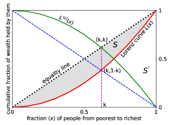
Figure 1: The Lorenz function $L(x)$ represents the fraction (curve shown in red) of overall income or wealth assumed by the poorer $x$ fraction of the people. The Gini index $g$ is given by the ratio of the area that lies between the line of equality and Lorenz curve over the total area under the line of equality ($g=2S$). The complementary Lorenz function $L^{c}(x)\equiv 1-L(x)$ is represented here by the green curve. The $k$ index value is given by the fixed point $L^{c}(k)=k$ of $L^{c}(x)$.

III Models and Simulation Results

In this section, we will discuss the numerical studies of the kinetic exchange models of income distribution (among agents or traders having saving propensities $\lambda$), employing two kinds of dynamics. In subsection III.1, the exchange occurs between randomly chosen pairs of agents with uniform saving behavior $0\leq\lambda<1$, which is fixed over time (here the most probable income in the steady-state increases with increasing saving propensity $\lambda$; see chakraborti2000statistical ). In III.2, one of the agents or traders in the chosen pair is the poorest in the whole population at that point of time (trade, exchange, or scattering) while the other one is randomly picked up from the rest, with the agents having a uniform saving propensity $0\leq\lambda<1$, fixed over time (where, in the steady-state, a self-organized minimum poverty level or SOPL of income or wealth appears, see ghosh2011threshold for agents with saving propensity $\lambda=0$). Here we show that SOPL increases with increasing $\lambda$. In subsection III.3, we revisit the trade dynamics where the exchange occurs between randomly chosen pairs of agents with the modification that $\lambda$ for each agent can take two values, zero (with probability $1-\rho$, $\rho<1$) or unity (with probability $\rho$), and it changes randomly over time or trade. Finally, in subsection III.4 the saving behaviour followed is that described in subsection III.3 but with the trading dynamics described in subsection III.2, the one that produces a self-organized poverty level.

We perform numerical simulations with fixed number of agents $N$ and total money $M=N$ for both the models. In our simulation, one Monte Carlo step is equivalent to $N$ pairwise exchanges. We take $N=1000$ agents and total money $M=N$, initially distributed over all the agents uniformly. The steady state distribution is measured over $10^{3}$ Monte Carlo time steps after relaxing $10^{6}$ Monte Carlo time steps for equilibration.

III.1 Uniform saving income exchange models and inequality indices

In this model, we consider a conserved system where total money $M$ and total agents $N$ are fixed. Each agent i possesses money $m_{i}(t)$ at a time t and in any interaction, a pair of agents i and j exchange their money such that their total money is conserved. For fixed saving propensity $\lambda$ of the agents, the exchange of money between two randomly chosen pairs can be expressed as

$$\begin{split}m_{i}(t+1)&=\lambda m_{i}(t)+\epsilon_{ij}((1-\lambda)(m_{i}(t)+m_{j}(t)))\\ m_{j}(t+1)&=\lambda m_{j}(t)+(1-\epsilon_{ij})((1-\lambda)(m_{i}(t)+m_{j}(t)))\end{split}$$ (1)

where $0\leq\epsilon_{ij}\leq 1$ is a random fraction varying in every interaction.

The steady state income distribution $P(m)$ for fixed saving propensity $\lambda$ is shown in Fig. 2(a). For $\lambda=0$, the steady state follows a Gibbs distribution and Most Probable Income (MPI) distribution is at MPI= 0. MPI per agent shifts from m = 0 to m = 1 as $\lambda\to 1$. Furthermore, the plot in semi-log (as shown in Fig. 2(a) inset) indicates an exponential nature for the tail end of the distribution.

In plot 2(b), we show the variation of the Kolkata index ($k$), the Gini index ($g$) and the Most Probable Income (MPI) against saving propensity $\lambda$. The Gini coefficient value diminishes from $0.5$ to $0$ as $\lambda$ approaches from $0$ to $1$. Similarly the $k$-index value reduces from $0.68$ to $0.5$ as $\lambda$ approaches from $0$ to $1$.

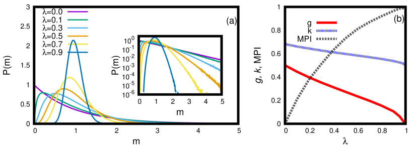
Figure 2: The pure kinetic exchange dynamics: (a) The steady state income distributions P(m) for different saving propensity $\lambda$ are shown in the plot. (Inset) The same distributions are shown in semi-log scale indicating an exponential nature of the tail end of the distributions. (b) The variation of Kolkata index ($k$), Gini index ($g$) and Most Probable Income (MPI) are shown against fixed saving propensity $\lambda$ (maximum value of $\lambda$ is $1_{-}$).

III.2 Self-organized minimum poverty level model and inequality indices

Here we consider a model where one of the agents in the chosen pair is necessarily the poorest at that point of time and the other one is randomly chosen from the rest. Here we vary $\lambda$ for values other than 0, as shown in Fig. 3. The exchange of money will follow the same rule as described by Eqn. 1. An important observation that ensues from the $\lambda\neq 0$ curves is that the MPI displaces to the right of the spectrum and shifts close to $m=1$ (resembling the nature of $P(m)$ against $m$ in Fig. 2). Here we also observe that the SOPL (below which $P(m)=0$) increases with increasing values of $\lambda$.

In Fig. 3(a), the steady state income distribution $P(m)$ for different $\lambda$ values are shown and the same distributions are shown in semi-log scale in the inset indicating an exponential nature of the tail end of the distributions. In Fig. 3(b), the variation of Kolkata index ($k$), Gini index ($g$) and Self-Organized Poverty-Line or SOPL are shown against saving propensity $\lambda$. The figure indicates that inequality of the distribution diminishing as $\lambda\to 1$ and also Self-Organized Poverty-Line or SOPL is rising to 1 as $\lambda\to 1$.

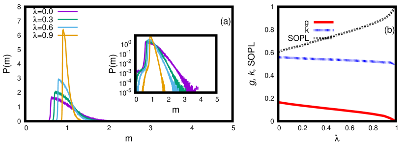
Figure 3: Self-Organized Poverty Level model: (a) Steady state income distribution $P(m)$ for fixed saving propensity $\lambda$ are shown. (Inset) The same distributions are shown in semi-log scale indicating an exponential nature of the tail end of the distributions. (b) The variation of the Kolkata index ($k$), the Gini index ($g$) and location of the Self-Organized Poverty Level (SOPL) are shown against fixed saving propensity $\lambda$ (maximum value of $\lambda=1_{-}$).

III.3 Indices for pure kinetic exchange model with two choices of $\lambda$

A more realistic saving behavior in a society would definitely mean that $\lambda$ should vary over time as it is heavily dependent on an individual’s saving interests. Thus, a randomness attached to the saving propensity in the form of a probability factor $\rho$ can act as an additional parameter in determining the nature of the wealth distribution curve. With this in mind, we consider exchange dynamics similar to that described in subsection III.1, but with a slight modification of Eqn. (1) as follows:

$$\begin{split}m_{i}(t+1)=\lambda_{\rho}m_{i}(t)+\epsilon_{ij}((1-\lambda_{\rho})(m_{i}(t)+m_{j}(t)))\\ m_{j}(t+1)=\lambda_{\rho}m_{j}(t)+(1-\epsilon_{ij})((1-\lambda_{\rho})(m_{i}(t)+m_{j}(t)))\end{split}$$ (2)

using $\lambda_{\rho}=1$ with probability $\rho$ and $\lambda_{\rho}=0$ with probability $1-\rho$; $\rho<1$. Henceforth we will refer to $\lambda_{\rho}$ as $\lambda$, without loss of generality and provided Eqn. 2 is satisfied.

Eqn. 2 suggests that each agent has two choices of $\lambda$ over time. In our study, the agents can take the saving propensity either 1 (with probability $\rho$) or 0 (with probability $1-\rho$) over time. For $\lambda$ strictly equal to 1, the exchange dynamics stops and hence values of $\lambda$ infinitesimally close to 1 are considered for simulations.

In Fig. 4(a), the steady state income distribution $P(m)$ is shown for different probability $\rho$. We observe that the most probable income (MPI) occurs at $m=0$, and the semi-log plots of the distributions indicate the exponential nature of the tail end of the distribution (see inset of Fig. 4(a)). The Kolkata index ($k$) and Gini index ($g$) rise slowly against $\rho$ (see Fig. 4(b)).

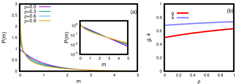
Figure 4: The pure kinetic exchange model of two choices of $\lambda$. (a) Steady state income distribution $P(m)$ for fixed saving propensity $\lambda$ are shown. (Inset) The same distributions are shown in semi-log scale indicating an exponential nature of the tail end of the distributions. (b) The variation of Kolkata index ($k$) and Gini index ($g$) are shown against the probability for taking $\lambda=1$ i.e. $\rho$ (maximum value of $\rho=1_{-}$).

III.4 Self-organized minimum poverty level model: Indices for two choices of $\lambda$

As before, we consider the same dynamics as described in subsection III.2 but the difference is that each agent has two choices of $\lambda$ over time. In our study, the agents can take the saving propensity either 1 (with probability $\rho$) or $0$ (with probability $1-\rho$) over time and we assume that the poorest agent trades with any of the agents in the rest of the population, which not only leads to a finite MPI but also a self organization in the system leading to an SOPL. In Fig. 5(a), the steady state income distribution $P(m)$ is shown for different probability $\rho$. The semi-log plots of the distributions indicate the exponential nature of the distribution (see inset of Fig. 5(a)). The variation of Kolkata index ($k$) and Gini index ($g$) and Self-Organized Poverty-Line or SOPL are shown against $\rho$ in Fig. 5(b). A very slow increasing trend of the inequality indices with $\rho$ can be observed here. Also the SOPL of the distribution slowly decreases against $\rho$.

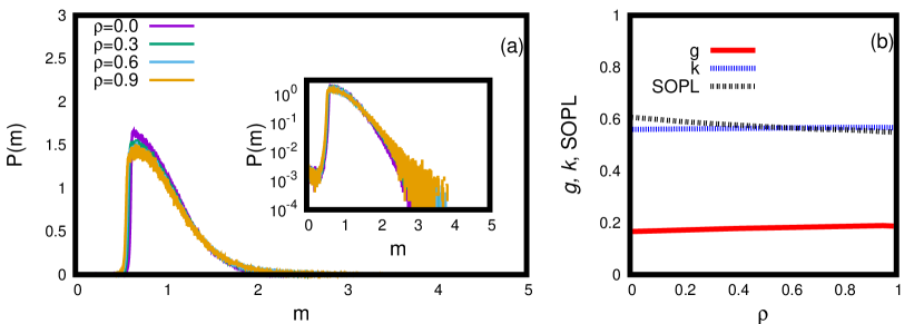
Figure 5: A self-organized minimum poverty level

model for two choices of saving propensity: (a) The steady state income distribution $P(m)$ for fixed saving propensity $\lambda$ is shown. (Inset) The same distributions are shown in semi-log scale indicating an exponential nature of the tail end of the distributions. (b) The variation of the Kolkata index ($k$), the Gini index ($g$) and the Self-Organized Poverty-Line or SOPL are shown against fixed saving propensity $\lambda$. A very slow increasing trend of the inequality indices and a slow decreasing trend of SOPL against $\rho$ can be observed here (maximum value of $\rho=1_{-}$).

IV Summary & Discussion

Income and wealth inequality in human societies has been ubiquitous over the history of mankind, very well recognized and has long been studied by philosophers and economists (see e.g., champernowne1998economic ; piketty2013capital for some recent discussions by economists). Recently, physicists have also joined the investigations on income and wealth inequalities (see e.g, chakrabarti2013econophysics ; pareschi2013interacting ; sen2014sociophysics for some detailed discussions and ludwig2021physics for an interesting application in the context of US economic inequalities during 1983-2018) essentially using kinetic theory or specifically kinetic exchange models (the key theme of this special issue).

In this paper, we have numerically studied the variations of income or wealth distribution $P(m)$ generated from the kinetic exchange models described earlier in section III and extracted the variations in the values of Gini $g$ and Kolkata $k$ indices with the saving propensity $\lambda$ of the agents, with two different kinds of trade or (kinetic) exchange dynamics. Along with the nature of steady state distributions $P(m)$, we have also studied the variations in the values of the inequality indices ($g$ and $k$) and the location of the Most Probable Income (MPI) or the Self-Organized Poverty Level (SOPL, if any) of income or wealth as the saving propensity $\lambda$ of the agents (fixed over time) and as the time fraction $\rho$ of choosing the saving propensity $\lambda=1$ over the other choice $\lambda=0$. Although two of the versions of the models (discussed in subsections III.1 and III.2) were addressed in earlier studies, the results for the variations of Gini ($g$) and Kolkata ($k$) indices with the saving propensity ($\lambda$) of the agents are new. The decrease in the inequality indices re-establish the models as sustainable market models where sheer self-interest in saving a portion of the money traded by each individual locally can cause a global peaked wealth distribution, where most agents prosper with finite money. We note in subsection III.3, where pair of traders are chosen randomly, and for the case discussed in subsection III.4, where the poorest agent is one of the partners in trade that both $g$ and $k$ increase (see Fig 4b) and SOPL decreases weakly (see Fig. 5b). These are probably justified because as $\rho$ increases, interactions with fully corrupt persons (having $\lambda=1$, who accumulate money in each trade and spend nothing) become more frequent. However, an important observation is that after introducing the constraint of selecting at least one agent with minimum money, an SOPL emerges (Fig. 5a) and so does an MPI replacing the $\lambda=0$ exponential to a Gamma-like distribution for all values of $\rho$. Hence an incentivized trading process for the poor, with just offering them greater opportunity to trade without supporting them with extra wealth, works greatly in raising the minimum wealth possessed by a population to a threshold money.

As shown in Figs. 2-5, the most-probable income or MPI (where $P(m)$ is highest) or the self-organized poverty level, the SOPL (below which $P(m)=0$ and usually the MPI coincides with the SOPL) increases with increasing saving propensity or $\lambda$. Generally speaking, in all these fixed saving propensity cases (see Figs. 2 and 3), the income or wealth inequalities, as measured by the index values of Gini $g$ and Kolkata $k$ (= 0.5 and $\simeq$ 0.68 respectively, in the pure kinetic exchange or Gibbs case, discussed analytically in the Introduction) decreases with increasing saving propensity ($\lambda$) of the agents.

Economic policy prescriptions naturally aim for reduced economic inequalities (see e.g., venkatasubramanian2017much for some discussions on the limits of equality imposed by thermodynamic and physical considerations). In this context, as our study indicates, reduction in the values of both the Gini and the Kolkata indices and increase in the value of the self-organized poverty level with increasing saving propensities of the agents, look quite encouraging. In particular, it should help in building and studying more specific kinetic exchange models with useful economic policy implications.

References

- [1] Sitabhra Sinha, Arnab Chatterjee, Anirban Chakraborti, and Bikas K Chakrabarti. Econophysics: An Introduction. John Wiley & Sons, 2010.
- [2] Bikas K Chakrabarti, Anirban Chakraborti, and Arnab Chatterjee. Econophysics and Sociophysics: Trends and Perspectives. John Wiley & Sons, 2006.
- [3] Victor M Yakovenko and J Barkley Rosser Jr. Colloquium: Statistical mechanics of money, wealth, and income. Reviews of modern physics, 81(4):1703, 2009.
- [4] Bikas K Chakrabarti, Anirban Chakraborti, Satya R Chakravarty, and Arnab Chatterjee. Econophysics of Income and Wealth Distributions. Cambridge University Press, 2013.
- [5] Lorenzo Pareschi and Giuseppe Toscani. Interacting Multiagent Systems: Kinetic Equations and Monte Carlo Methods. Oxford University Press, 2013.
- [6] Marcelo Byrro Ribeiro. Income Distribution Dynamics of Economic Systems: An Econophysical Approach. Cambridge University Press, 2020.
- [7] Parongama Sen and Bikas K Chakrabarti. Sociophysics: An Introduction. Oxford University Press, 2014.
- [8] Serge Galam. Sociophysics. Springer, Heidelberg, 2012.
- [9] Anirban Chakraborti and Bikas K Chakrabarti. Statistical mechanics of money: how saving propensity affects its distribution. The European Physical Journal B-Condensed Matter and Complex Systems, 17(1):167–170, 2000.
- [10] Arnab Chatterjee, Bikas K Chakrabarti, and SS Manna. Pareto law in a kinetic model of market with random saving propensity. Physica A: Statistical Mechanics and its Applications, 335(1-2):155–163, 2004.
- [11] Arnab Chatterjee and Bikas K Chakrabarti. Kinetic exchange models for income and wealth distributions. The European Physical Journal B, 60(2):135–149, 2007.
- [12] Salete Pianegonda, Jose Rroberto Iglesias, Guillermo Abramson, and JL Vega. Wealth redistribution with conservative exchanges. Physica A: Statistical Mechanics and its Applications, 322:667–675, 2003.
- [13] Asim Ghosh, Urna Basu, Anirban Chakraborti, and Bikas K Chakrabarti. Threshold-induced phase transition in kinetic exchange models. Physical Review E, 83(6):061130, 2011.
- [14] Jose Rroberto Iglesias. How simple regulations can greatly reduce inequality. arXiv:1007.0461; Science & Culture, 76:437–443, 2010.
- [15] Bikas K Chakrabarti and Antika Sinha. Development of econophysics: A biased account and perspective from kolkata. Entropy, 23(2):254, 2021.
- [16] Suchismita Banerjee, Bikas K Chakrabarti, Manipushpak Mitra, and Suresh Mutuswami. Inequality measures: The kolkata index in comparison with other measures. Frontiers in Physics, 8:562182, 2020.
- [17] Antika Sinha, Sudip Mukherjee, and Bikas K Chakrabarti. Econophysics through computation. arXiv:2001.04188; Journal of Physics Through Computation, 3(1):1–54, 2020.
- [18] Asim Ghosh, Nachiketa Chattopadhyay, and Bikas K Chakrabarti. Inequality in societies, academic institutions and science journals: Gini and k-indices. Physica A: Statistical Mechanics and its Applications, 410:30–34, 2014.
- [19] Bruce J West and Paolo Grigolini. Crucial Events: Why are Catastrophes Never Expected? World Scientific, 2021.
- [20] David Gawen Champernowne and Frank Alan Cowell. Economic Inequality and Income Distribution. Cambridge University Press, 1999.
- [21] Thomas Piketty. Capital in the Twenty-First Century. Harvard University Press, 2013.
- [22] Danial Ludwig and Victor M Yakovenko. Physics-inspired analysis of the two-class income distribution in the usa in 1983-2018. arXiv preprint arXiv:2110.03140; To be published in this Theme Issue., 2021.
- [23] Venkat Venkatasubramanian. How Much Inequality Is Fair? Columbia University Press, 2017.