Analytical simulations of the effect of satellite constellations on optical and near-infrared observations

Abstract

Context. The number of satellites in low-Earth orbit is increasing rapidly, and many tens of thousands of them are expected to be launched in the coming years. There is a strong concern among the astronomical community about the contamination of optical and near-infrared observations by satellite trails. Initial investigations of the impact of large satellite constellations have been presented in Hainaut & Williams (2020) and McDowell (2020), among others.

Aims. We expand the impact analysis of such constellations on optical and near-infrared astronomical observations in a more rigorous and quantitative way, using updated constellation information, and considering imagers and spectrographs and their very different characteristics.

Methods. We introduce an analytical method that allows us to rapidly and accurately evaluate the effect of a very large number of satellites, accounting for their magnitudes and the effect of trailing of the satellite image during the exposure. We use this to evaluate the impact on a series of representative instruments, including imagers (traditional narrow field instruments, wide-field survey cameras, and astro-photographic cameras) and spectrographs (long-slit and fibre-fed), taking into account their limiting magnitude.

Results. As already known (Walker et al., 2020), the effect of satellite trails is more damaging for high-altitude satellites, on wide-field instruments, or essentially during the first and last hours of the night. Thanks to their brighter limiting magnitudes, low- and mid-resolution spectrographs will be less affected, but the contamination will be at about the same level as that of the science signal, introducing additional challenges. High-resolution spectrographs will essentially be immune. We propose a series of mitigating measures, including one that uses the described simulation method to optimize the scheduling of the observations. We conclude that no single mitigation measure will solve the problem of satellite trails for all instruments and all science cases.

1 Introduction: Satellite constellations

In the most general sense, a constellation of artificial satellites is a set of spacecraft that share a common design, distributed among different orbits to provide a service and/or a land coverage that cannot be achieved by means of just one single satellite. Satellite constellations have been in use since the early times of the space age and their applications range from telecommunications (civil or military, e.g. the Molniya series), meteorology (Meteosat), remote sensing (as the two-satellite constellations Sentinel of ESA) or global navigation satellite systems (GNSS; GPS, Glonass, Galileo or Beidou systems).

Until recently, the satellite constellation with a largest number of elements was the Iridium system, with some 70 satellites in low-Earth orbit (LEO, altitude less than 2000 km), aimed to provide cell phone services with worldwide coverage. The so-called Iridium flares caused by reflected sunlight from the flat antennae of the first generation of Iridium satellites awoke the awareness of the astronomical community about possible deleterious effects of satellite constellations on astronomical observations, both optical and in radio (James, 1998). Global navigation satellites systems also require worldwide coverage that, in this case, can be achieved with smaller constellations, typically of the order of 30 satellites, placed at higher orbits ($\sim 20\,000$ km).

For the purpose of this paper we consider a mega-constellation to refer to any satellite constellation made up from a number of satellites significantly larger than the Iridium constellation, say in excess of 100 satellites. Several such systems have been proposed during the last decade, in all cases with the purpose to provide fast internet access worldwide. The technical requirements for that application (large two-way bandwidth, short delay time, large number of potential users) lead to designs of constellations made up from huge numbers of satellites, counted in the thousands, placed at low-Earth orbit.

The contrast with traditional constellations is overwhelming. The examples mentioned above, or the plans to launch new constellations of nano- and pico-satellites, imply challenges of their own and contribute to the issues of orbital crowding, space debris management, radioelectric noise, etc., but they imply numbers of satellites orders of magnitude smaller and, most often, with elements much fainter, than the mega-constellations discussed in here.

Several new generation mega-constellations are in the planning stages, and some number of satellites of two of these constellations, namely SpaceX’s Starlink and OneWeb, have already been placed in orbit. In Table 1 we list some of the planned constellation configurations for which information is publicly available. Several more satellite operators indicated their intentions to build about a dozen of additional similar constellations. Many companies are also planning constellations of much smaller satellites (cubesats, nanosats…), which are less relevant for optical astronomy. We note that satellite operators, even those with satellites already in orbit, frequently modify the configuration of their constellation projects. Furthermore, other satellite operators have indicated their intentions to launch mega-constellations, but without so far submitting any application or publishing any details. Therefore, the configurations used in this paper should be treated as a representative, and their impact on astronomical observations obtained from the following simulations and their interpretation are an illustration of the situation as it could be in the late 2020’s. In first approximation, the numbers scale linearly with the total number of satellites in the constellation, so the effects be scaled.

Of all these projects, the SpaceX Starlink constellation is clearly in the forefront. Since the launch of their first group of satellites in May 2019, the trains of very bright pearls that form the satellites illuminated by the Sun have caught the attention even of the general public, and have triggered the alarms of the astronomical community (see, for example Witze, 2019). These bright trains are formed only at the first stages of the deployment of each Starlink launch, with the satellites becoming fainter as they later climb to the final operational orbits, and attain an operational attitude that reduces their apparent brightness.

Our aim in this paper is to assess the impact of satellite mega-constellations on optical and near-infrared astronomy from computer simulations of two kinds. Such simulations are described in §2, where we depict the usual discrete simulations and, also, a new approach consisting on formulating statistical predictions from analytical probability density functions that describe the main properties of the constellations. The same section includes consideration on how to estimate the apparent brightness of satellites illuminated by sunlight, with special attention to the concept of effective magnitude.

The effect on observations is addressed in §3. There we provide details on the specific details of a set of simulations, their implications for several observing modes (direct imaging and spectroscopy, including multi-fiber instruments) and we discuss some possibilities to mitigate the impact in §4. The appendix includes the details on how the equations of our analytical model are derived.

Table 1: Orbit configurations for the satellite constellations considered in this paper, totaling almost 60 thousand satellites, providing the orbital altitude and inclination, number of satellites within an orbital plane $n_{\mathrm{sat}}$ and the number of orbital planes $n_{\mathrm{plane}}$ making up the constellation (consisting of $n_{\mathrm{sat}}\times n_{\mathrm{plane}}$ satellites). These are the constellations for which supporting information is available. These constellations are therefore to be considered as representative of a plausible situation by $\sim 2030$, but the exact details of the distribution of satellites may be different.

Altitude	Inclination	$n_{\mathrm{sat}}$	$n_{\mathrm{plane}}$	$n_{\mathrm{sat}}\times n_{\mathrm{plane}}$
Starlink Generation 1 11926 satellites
$550$ km	$53\degr$	22	72	1584
$540$ km	$53\aas@@fstack{\circ}2$	22	72	1584
$570$ km	$70\degr$	20	36	720
$560$ km	$97\aas@@fstack{\circ}6$	58	6	348
$560$ km	$97\aas@@fstack{\circ}6$	43	4	172
$335.9$ km	$42\degr$	60	42	2493
$340.8$ km	$48\degr$	60	42	2478
$345.6$ km	$53\degr$	60	42	2547
Starlink Generation 2 30000 satellites
$328$ km	$30\degr$	1	7178	7178
$334$ km	$40\degr$	1	7178	7178
$345$ km	$53\degr$	1	7178	7178
$360$ km	$96\aas@@fstack{\circ}9$	50	40	2000
$373$ km	$75\degr$	1	1998	1998
$499$ km	$53\degr$	1	4000	4000
$604$ km	$148\degr$	12	12	144
$614$ km	$115\aas@@fstack{\circ}7$	18	18	324
Amazon Kuiper 3236 satellites
$630$ km	$51\aas@@fstack{\circ}9$	34	34	1156
$610$ km	$42\degr$	36	36	1296
$590$ km	$33\degr$	28	28	784
OneWeb Phase 1 1980 satellites
$1200$ km	$87\aas@@fstack{\circ}9$	55	36	1980
OneWeb Phase 2 revised 6372 satellites
$1200$ km	$87\aas@@fstack{\circ}9$	49	36	1764
$1200$ km	$40\degr$	72	32	2304
$1200$ km	$55\degr$	72	32	2304
GuoWang GW-A59 12992 satellites
$590$ km	$85\degr$	60	8	480
$600$ km	$50\degr$	50	40	2000
$508$ km	$55\degr$	60	60	3600
$1145$ km	$30\degr$	64	27	1728
$1145$ km	$40\degr$	64	27	1728
$1145$ km	$50\degr$	64	27	1728
$1145$ km	$60\degr$	64	27	1728

2 Simulations

2.1 Visibility

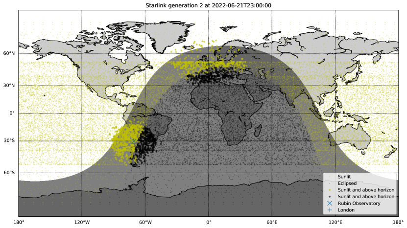
Figure 1: A discrete realization of the Starlink Generation 2 constellation overlaid on a map of Earth. The day and night sides of Earth are shown for 2022 June 21 at 23:00UTC, near the June solstice. Satellites are shown as either sunlit (yellow), or eclipsed by the Earth (black) and above the horizon for two geographical locations, Vera Rubin Observatory in Chile (latitude $-30\degr$), and London in the United Kingdom (latitude $\sim 50\degr$). Over-densities of satellites in geographic latitude $b$ are visible at latitudes $|b|=30^{\circ}$, $40^{\circ}$ and $53^{\circ}$, corresponding to the inclination of the most populous orbital shells. Due to their orbital altitudes, satellites remain visible for locations where the Sun is below the horizon, and will remain visible throughout all the night for locations at high geographical latitudes.

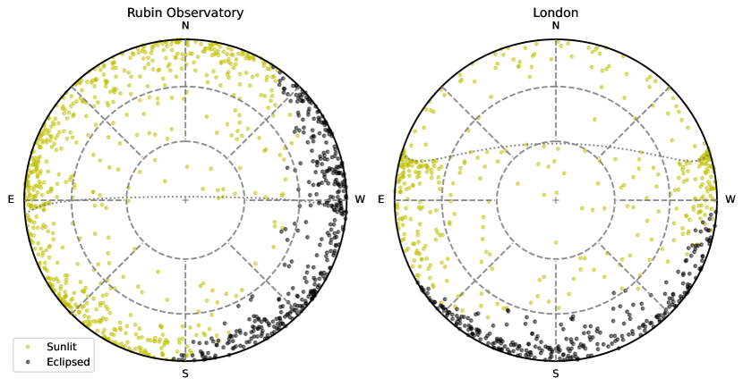
Figure 2: A discrete realization of the Starlink Generation 2 constellation plotted on all sky maps representing the sky above Vera Rubin Observatory (left) and London (right). Satellites are shown as sunlit (yellow) or eclipsed by the Earth (black). The number of satellites increases towards the horizon because, for a given solid angle, looking at lower elevations from the horizon the distance to the shell surface increases and, hence, the field of view contains larger portions of the orbital shells. Due to the orbital inclination and orbital altitude of the orbital shells, over-densities of satellites are also present in these maps. The map for London shows this very clearly for the two orbital shells with $i=53^{\circ}$ and $h=345$ km (7178 satellites) and 499 km (4000 satellites), where more satellites are present south from the dotted line. The dotted line in the all sky map for Vera Rubin Observatory is for the orbital shell with $i=30^{\circ}$, $h=328$ km, with a larger number of satellites north from that line.

A satellite will be visible at optical and near-infrared wavelengths if it is above the horizon for the geographical location of the observer and if it is illuminated by the Sun, making it to reflect and diffuse sunlight back to the observer. Hence, the visibility of a given satellite will depend upon its location within its orbit, the geographic location of the observer, and the location of the Sun, all as a function of time.

While the motion of a satellite in the Earth’s gravitational field and through the higher residual layers of the atmosphere is usually computed through either numerical integration or using simplified analytical models (e.g. Montenbruck & Gill, 2000; Vallado et al., 2006), these offer an accuracy that is not required for the statistical results that we want to derive from the simulations presented here. Instead, we assume that the satellites move in circular Keplerian orbits, and we will neglect the effects of atmospheric drag, the lack of spherical symmetry of the Earth’s gravitational potential and perturbations by the Sun and the Moon. Furthermore, for simplicity, satellite positions are defined in an inertial geocentric reference system (Celestial Intermediate Reference System), neglecting the small effects of precession, nutation and Earth orientation parameters. These assumptions allow us to consider only the idealised motion of the satellites, the motion of the observer (uniform Earth rotation) and the apparent motion of the Sun.

Satellite constellations for worldwide coverage are generally configured as Walker constellations (Walker, 1984). Here, satellites are in circular orbits of distinct orbital shells, with each shell described by its orbital altitude $h_{\mathrm{sat}}$ and orbital inclination $i$. Within each shell, equally spaced orbital planes are populated by satellites, also equally spaced within each plane. In Table 1 we use $n_{\mathrm{sat}}$ to denote the number of satellites in a single orbital plane, and $n_{\mathrm{plane}}$ to indicate the number of orbital planes. The total number of satellites within each shell is $N_{\mathrm{sat}}=n_{\mathrm{sat}}\times n_{\mathrm{plane}}$, and the total number of satellites in a constellation the sum of the number of satellites in each shell.

In this paper we consider only idealized, complete constellations. Individual satellites, as well as the trains of satellites in very low orbits right after launch and the satellites in near-to-re-entry orbits, are not considered. Even taking into account the large number of launches required to replenish the constellations, and the hopefully equally large number of satellites on end-of-life orbits, the number of such satellites will be one to two orders of magnitude smaller than the number of satellites in operations. Also, as these satellites are in lower orbits their impact is concentrated during the very beginning and end of night. Hence, their contribution to the overall situation caused by the constellations in operation is therefore small.

We expand on the work by Hainaut & Williams (2020), who used a simplistic geometric approximation to estimate the density of satellites and their effects. That model had the advantage of being extremely fast and numerically lean, and to yield acceptable results for mid-latitude observatories, but it had the major shortcoming not to account for latitude effects. This aspect is rigorously addressed in the following sections.

2.1.1 Discrete simulations

To obtain a realization of a satellite constellation at a given time, the positions and velocities of all satellites in the constellation are computed using the assumptions listed earlier. Figure 1 shows such a realization for the Starlink Generation 2 constellation on a map of the Earth near the June solstice when the Sun is at its highest northern declination. Hence, for locations at high geographical latitudes in the northern hemisphere, satellites will be visible throughout the whole night, whereas for lower latitudes and in the southern hemisphere satellites will only be visible around twilight. This figure depicts over-densities of satellites at geographical latitudes near the orbital inclination of different orbital shells.

These over-densities are also seen in the all-sky maps shown in Fig. 2 for two locations, the Vera Rubin Observatory (VRO) at Cerro Pachón in Chile (at latitude $-30\degr$), and London in the United Kingdom (at latitude $+50\degr$). The increased distance to the orbital shells when looking at lower elevations above the horizon leads to larger sampling volumes, which explains that these all-sky maps show increasing satellite densities towards the horizon, though additional over-densities exist near the projected location of the northern and southern limits of the most populous orbital shells.

This discrete approach has been followed to assess the impact of satellite constellations in terms of the amount of them that are visible during the night above a given elevation from the horizon, as shown, for instance, in McDowell (2020). To this end, a specific constellation is selected (in terms of shell number and, for each of them, the altitude, orbital inclination and number of satellites), an observatory location is specified (in general only latitude is relevant) and the illumination conditions are fixed through Sun declination and hour angle. The simulation of the Keplerian movement of each satellite of the constellation allows counting the number of satellites that are above a specific elevation and their illumination conditions (sunlit or eclipsed). Additional considerations may allow computing some photometric estimates (§2.2). This kind of discrete, all-sky simulations may be iterated, including some random initialisation of parameters at each run to average-out systematic effects due to the spatial and temporal texture induced by the constellation structure.

2.1.2 Number of satellite trails in an observation

Besides the all-sky simulations, an observation-oriented approach is also needed. This requires specifying all the parameters required for the all-sky simulations and, also, selecting the observation direction (azimuth, elevation), field-of-view (FOV) and exposure time of an observation. In these observations, the motion of the satellite during the exposure will leave a satellite trail on the images. Repeating this simulation leads to the average estimate of the number of satellite trails that would affect the observation. The geometry of the problem allows also computing the position angle of the trails and the apparent angular velocity of each satellite that crosses the FOV.

In Fig. 3 we show the results of a discrete simulation on observations with different exposure times and fields-of-view. The discrete simulation used a constellation of 10 000 satellites in a single orbital shell of 100 orbital planes with 100 satellites within each plane, at 1000 km altitude and $53\degr$ inclination. For an observer at $-30\degr$ latitude, the number of satellite trails visible within an observation of an exposure time and circular field-of-view towards zenith were counted and averaged over 1000 simulations.

The simulations show a dependence with both field-of-view and exposure time (solid dots). This relation can be understood as the number of satellites present at the start of the exposure, plus those travelling through the field-of-view during the exposure, and has the form

$$N_{\mathrm{trail}}=\rho_{\mathrm{sat}}(A_{\mathrm{fov}}+L_{\mathrm{fov}}\omega_{\mathrm{sat}}t_{\mathrm{exp}}).$$ (1)

Here, $\rho_{\mathrm{sat}}$ is the instantaneous satellite number density, i.e. the number of satellites per unit area on the sky, and $\omega_{\mathrm{sat}}$ the angular velocity of the satellites in the direction of the exposure. The exposure itself has field-of-view area of $A_{\mathrm{fov}}$ and width $L_{\mathrm{fov}}$, and exposure time $t_{\mathrm{eff}}$. For comparison with the simulations we use a field-of-view with a circular radius $R_{\mathrm{fov}}$, such that $A_{\mathrm{fov}}=\pi R_{\mathrm{fov}}^{2}$ and $L_{\mathrm{fov}}=2R_{\mathrm{fov}}$.

The simulations provide the instantaneous satellite density $\rho_{\mathrm{sat}}$ and the average angular velocity $\omega_{\mathrm{sat}}$ and using these values, Eqn. 1 provides the predicted number of trails for the different observation parameters, plotted as lines in Fig. 3. The predictions match the simulations, though for short exposures and/or small fields-of-view, the simulations suffer from noise due to the few satellites passing through the observation.

Equation 1 is valid for a single shell in a constellation, as the instantaneous density $\rho_{\mathrm{sat}}$ and angular velocity $\omega_{\mathrm{sat}}$ depend on the properties of the shell. To obtain the total number of trails in an observation for a satellite constellation with multiple shells, Eqn. 1 can be computed for each shell, and the results summed.

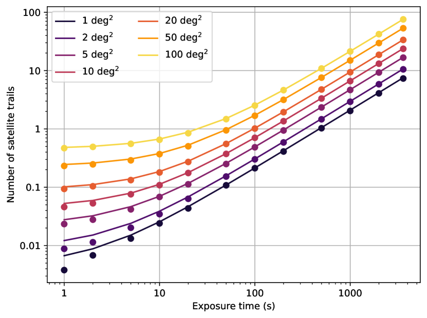
Figure 3: The number of satellites visible in an exposure depending on the exposure time $t_{\mathrm{exp}}$, and the instrument field-of-view, specified by its circular radius $R_{\mathrm{fov}}=L/2$. The effect of a discrete constellation of $10\,000$ satellites in a single orbital shell of 100 orbital planes and 100 satellites per plane at 1000 km altitude and $53\degr$ inclination is simulated for an observer at $-30\degr$ latitude, observing towards zenith. The points are the results of the discrete simulations for different values of exposure time $t_{\mathrm{exp}}$ and field-of-view ($\pi R_{\mathrm{fov}}^{2}$). The solid lines are predictions based on Eqn. 1.

2.1.3 Analytical simulations

The averaging over many randomly initialized parameters of a satellite constellation for the discrete simulations is computationally expensive, and may lead to noise due to insufficient satellites passing through observations with small fields-of-view and/or short exposures to obtain a valid average (see Fig. 3). Given that the averaging over randomly initialized parameters has the effect of smoothing out the satellite locations within a given orbital shell, we instead treat the satellite locations as probability density functions, which have the advantage that these are analytical expressions.

Figure 1 shows that the satellite locations are uniformly spread in geocentric longitude, but strongly peaked towards geocentric latitudes $\phi$ close to the values equal to the orbital inclination $-i$ and $+i$ of a constellation shell. For a satellite at true anomaly (measured from the ascending node) $\kappa$, the geocentric latitude is given by $\sin\phi=\sin\kappa\sin i$, and its probability distribution follows the Arcsine probability distribution. For a single satellite at orbital altitude $h_{\mathrm{sat}}$, the probability density per unit surface area as a function of $\phi$ is:

$$P(\phi,i,h_{\mathrm{sat}})=\frac{1}{2\pi^{2}(R_{\oplus}+h_{\mathrm{sat}})^{2}\sqrt{(\sin i+\sin\phi)(\sin i-\sin\phi)}}.$$ (2)

Here $R_{\oplus}$ is the radius of the Earth, and this expression is valid for $|\phi|<i$, and zero otherwise. A detailed derivation of Eqn. 2 is given in Appendix A.1.

Equation 2 can be integrated over the surface of the orbital shell spanned by the field-of-view of an instrument from an observatory located on Earth to obtain the fraction of the sample present within the instrument field-of-view. For the remainder of the paper, we will make the simplifying assumption that $P(\phi,i,h_{\mathrm{sat}})$ is constant over the instrument field-of-view. This assumption will generally be true for the small fields-of-view under consideration in the remaining analysis. It has the advantage that it removes any dependence on the precise shape and orientation of the instrument field-of-view, and instead solely depends on the sky area covered by the field-of-view. The assumption allows us to evaluate Eqn. 2 for a line-of-sight (specified by azimuth and elevation) of the observation from an observatory on Earth intersecting the orbital shell at distance $d$ and with an impact angle $\alpha$ ($\alpha=90\degr$ at zenith and $\alpha<90\degr$ for lower elevations). The instantaneous surface density $\rho_{\mathrm{sat}}$ can then be obtained by scaling the probability by the surface area of the orbital shell covered an angular area $A$ of 1 square degree, providing

$$\rho_{\mathrm{sat}}=N_{\mathrm{sat}}P(\phi,i,h_{\mathrm{sat}})\frac{{d^{2}A}}{\cos\alpha},$$ (3)

where $N_{\mathrm{sat}}$ is the number of satellites in the orbital shell with inclination $i$ and orbital altitude $h_{\mathrm{sat}}$. Equations to derive the distance $d$ and impact angle $\alpha$ given the location of the observatory and azimuth and elevation of the observation are given in Appendixes A.2 and A.3.

The angular velocity of the satellites in an orbital shell towards the line-of-sight can be determined using the equations provided in Appendix A.4. Due to the rotation of the Earth within the orbital shell of a satellite constellation, the velocity vectors project differently on the sphere of the sky and hence satellites will have somewhat different angular velocities depending on their north- or southbound trajectory. Given that for a full constellation, an equal amount of satellites will be on northbound as well as southbound trajectories, we can take the average of both angular velocities to obtain $\omega_{\mathrm{sat}}$.

For a given satellite constellation, observatory latitude and observation parameters (field-of-view and exposure time), the analytical simulations predict the number of trails as a function of azimuth and elevation which is inherently static with time. The final step to complete the analytical simulation is taking into account the illumination of the different orbital shells by the Sun, as this modulates the visibility of a shell as a function of time of day and time of year. The impact of solar illumination is implemented by computing whether the intersection of a given line-of-sight with an orbital shell is in the shadow of the Earth or not. If the intersection point is located in the shadow, and the satellites are not visible, we set $N_{\mathrm{trail}}=0$ for that shell in the sum of satellite trails over the different orbital shells.

Figure 4 shows all sky maps using the analytical simulations, providing the number of satellite trails from Eqn. 1. The contribution of the different orbital shells of multiple satellite constellations is apparent, as is the impact of solar illumination.

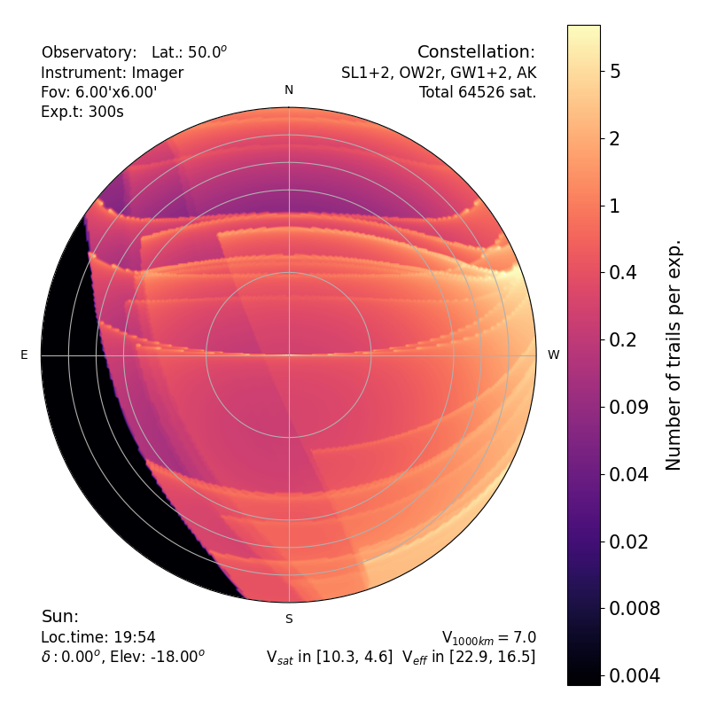
Figure 4: Sky maps with an example of the resulting number of trails per exposures. The circles mark $0\degr$, $10\degr$, $20\degr$, $30\degr$, and $60\degr$ elevation. The observatory is located at $+50\degr$ latitude; the sun at $-18\degr$ elevation; the camera has a FOV with diameter $L_{\mathrm{fov}}=6\arcmin$, and the exposure time is 300 s. The satellites are those from Table 1. In the black region at the South-East, all satellites are already in the shadow of the Earth. The edges running from North-East to South-West correspond to constellation shells at lower altitudes, whose South-East parts are already in the shadow. The sharp features running from East to West correspond to the edges of constellation shells whose inclinations are close to the observatory latitude.

2.2 Photometry

Providing a reliable estimation of the apparent brightness of the satellites is an obvious requirement for any model that intends to assess the impact of mega-constellations on astronomical observation. The celestial mechanics part of the problem admits an accurate solution that, even in a simplified frame (as described in §2.1.1 and §2.1.3), leads to sound predictions of the spatial parameters (satellite density and their motion). However, the photometric part of the problem faces additional difficulties, due to the complex geometrical and reflective properties of the satellite that, also, are different from one constellation to another.

In the visible and near-infrared (NIR), the light from the satellite is reflected sunlight with a specular and a diffuse component. The specular reflection happens on flat panels: antennas, satellite bus, possibly also solar panels (although while the satellites are in operations, these are perpendicular to the Sun). A complete and accurate representation of the reflection by a satellite would require detailed knowledge of the shape and material of the satellites (see Walker et al., 2020, for a summary of the state-of-the-art). A simplified model can be assembled from photometric observations covering a range of zenithal distance and solar illumination.

Empirical models (for instance, a flat panel model, Mallama, 2020a) are being developed, and theoretical approaches are also used to define photometric parameters of the satellites (Walker et al., 2020). However, as of today, the available observations are sufficient only for simplistic photometric models. Hopefully, dedicated observation campaigns will refine the characterization of the satellites in the coming years.

Table 2: Representative magnitudes of the satellites.

Satellite	Operational	Mag	Mag	Mag	$pr^{2}$	$p$	$r$	Ref.
	altitude	at op.	dispersion	at
	[km]	alt.		1000km	[m2]		[m]
Starlink original	550km	4.6	0.7	5.9	0.085	0.25	0.58	1
		4.0	0.7	5.3	0.152	0.25	0.78	2
		4.2	(model)	5.5	0.125	0.25	0.71	3
Starlink DarkSat	550km	5.1	(single)	6.4	0.056	0.08	0.71	4
Starlink VisorSat	550km	6.2	0.8	7.5	0.023	0.25	0.30	5
		5.8	0.6	7.1	0.028	0.25	0.33	6
OneWeb	1200	7.6	0.7	7.2	0.027	0.25	0.33	7

Notes: $p$ is the (arbitrary) geometric albedo used for the conversion of the cross-section $pr^{2}$ into an estimate of the radius $r$. References: 1: Mallama (2020b); 2: Krantz in Otarola et al. (2020); 3: value used in Hainaut & Williams (2020); 4: using the darkening of 0.88 mag on one DarkSat, from Tregloan-Reed et al. (2020); 5: median value from Mallama (2021); 6: average from Krantz in Otarola et al. (2020); 7: Mallama (2020c)

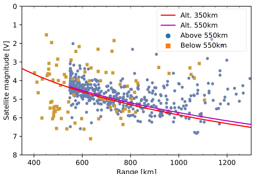
Figure 5: Magnitude of the satellites as a function of the range observer-satellite. The dots are measurements of original Starlink satellites (Pomenis telescope, from Otarola et al., 2020), and the lines are obtained using a simplified Lambertian sphere model for two altitudes. The unknown solar phase angle contributes to the dispersion of the measurements.

2.2.1 Apparent magnitude

The simple photometric model we use is based on the Lambertian sphere model. The theoretical foundations of the Lambertian sphere model can be seen, for instance, in Karttunen et al. (1996). The different specific formulations, such as those by Hainaut & Williams (2020) and McDowell (2020), can be unified under a single formula:

$$m_{\mathrm{sat}} = m_{\odot}-2.5\log_{10}\left(pR_{\mathrm{sat}}^{2}\right)+5\log_{10}\left(d_{\mathrm{sat}\odot}d_{\mathrm{sat}}\right)$$ (4)

$$-2.5\log_{10}\upsilon(\alpha_{\odot})+k\chi\leavevmode\nobreak\ .$$

In Eqn. 4, $m_{\odot}$ is the Sun’s apparent magnitude as seen from Earth, in the photometric band of interest. Typically, this is Johnson’s $V$ band, with $m_{\odot}=-26.75$. The second term considers the object’s intrinsic photometric properties: $pR_{\mathrm{sat}}^{2}$ is the photometric cross-section, with $p$ the object’s geometric albedo and $R_{\mathrm{sat}}$ the radius of the (spherical) satellite. The third term includes several distances: $d_{\mathrm{sat}\odot}$ is the distance from the satellite to the Sun, $d_{\mathrm{sat}}$ represents the distance from the observer to the satellite. For our problem, $d_{\mathrm{sat}\odot}=1$ AU. The fourth term is the correction for the solar phase $\alpha_{\odot}$. Finally, $k\chi$ represents the extinction term, $k$ being the extinction coefficient (in magnitudes per unit airmass), and $\chi$ the airmass (equal to $1/\sin{e_{\mathrm{sat}}}$ in the plane-parallel approximation, with $e_{\mathrm{sat}}$ representing the satellite’s elevation above the horizon; here, as we know the orbits of the object, we use the exact $\chi=d_{\mathrm{sat}}/h_{\mathrm{sat}}$). In the $V$ band, $k=0.12$ is a typical value (Patat et al., 2011).

For a Lambertian sphere, $\upsilon(\alpha_{\odot})=(1+\cos\alpha_{\odot})/2$. However, a large number of photometric measurements of Starlink original satellites (Mallama, 2020b) and Starlink VisorSat (Mallama, 2021) indicate an extremely weak dependency of the magnitude (corrected for distance and extinction) with the solar phase angle, a circumstance that has to be related to the morphology of the satellite, which is very different to a sphere. We therefore consider $\upsilon=1$, leading to

$$m_{\mathrm{sat}}=m_{\odot}+2.5\log_{10}d_{\mathrm{sat}}^{2}-2.5\log_{10}\left(pR_{\mathrm{sat}}^{2}\right)+kd_{\mathrm{sat}}/h_{\mathrm{sat}}\leavevmode\nobreak\ ,$$ (5)

where both $d_{\mathrm{sat}}$ and $R_{\mathrm{sat}}$ are expressed in the same units.

The photometric cross-section is the only parameter that depends on the satellite’s physical properties in this model. Hainaut & Williams (2020) adopted $pR_{\mathrm{sat}}^{2}=0.25$ $\mathrm{m}^{2}$ for the first-generation Starlink. In order to facilitate the comparisons between satellites, one introduces the absolute magnitude $m_{\mathrm{1000km}}$, normalized to a standard distance $d_{\mathrm{sat}}=1000$ km. With that value for $d_{\mathrm{sat}}$, Eqn. 5 becomes

$$m_{\mathrm{sat}}=m_{\mathrm{1000km}}+5\log_{10}\left(d_{\mathrm{sat}}/1000\right)+kd_{\mathrm{sat}}/h_{\mathrm{sat}}\leavevmode\nobreak\ ,$$ (6)

with $d_{\mathrm{sat}}$ expressed in km. Sometimes, $m_{\mathrm{550km}}=m_{\mathrm{1000km}}-1.3$ is used instead.

Table 2 lists the absolute magnitudes measured for different satellite types, and the corresponding photometric cross-section and visual magnitude at zenith. The dispersion of the measurements of $m_{\mathrm{1000km}}$ is around 0.7 mag; Fig. 5 shows an even wider dispersion. Consequently, the simplistic model presented above can only represent the general trend of the satellite magnitude, as illustrated by the comparison with observations (Fig. 5). In the simulations described below, we will use $m_{\mathrm{1000km}}=7$, equivalent to $m_{\mathrm{550km}}=5.7$.

2.2.2 Effective magnitude and limiting magnitude

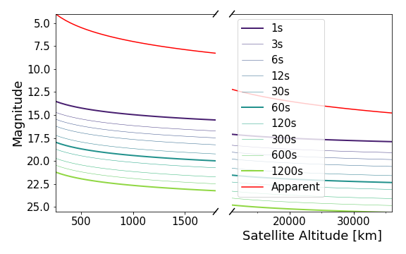
Figure 6: Visual (red) and effective magnitudes of a satellite at zenith, as a function of its altitude, for various exposure times (see legend). The satellite used is a Starlink VisorSat with $m_{\mathrm{1000km}}=7$, considered as a trailed point source.

a

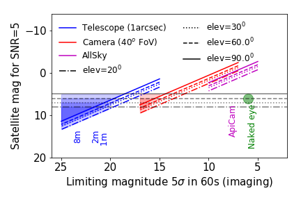
b

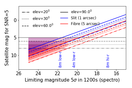
Figure 7: Detection limit for the satellite apparent magnitude as a function of the limiting magnitude of the instrument. a: the for an imager, the limiting magnitude corresponds to 5$\sigma$ in a 60s exposure time; b: for a spectrograph, the limiting magnitude corresponds to $5\sigma$ in a 1200s exposure. In both cases, various resolution element sizes are represented in different colour. Typical satellite apparent velocities corresponding to various elevations are represented with different line styles. A satellite will be detected if its apparent magnitude is in the shaded area above the coloured line corresponding to the considered elevation. The horizontal limit correspond to the typical brightest satellite at that elevation. Typical limiting magnitudes are indicated.

During an exposure of duration $t_{\mathrm{exp}}$, a satellite will leave a trail of length $\omega_{\mathrm{sat}}t_{\mathrm{exp}}$ (with $\omega_{\mathrm{sat}}$ being the apparent angular speed of the satellite), typically much longer than the FOV of the instrument. The signal corresponding to the apparent magnitude is therefore spread along the length of the trail. The count level on the detector amounts to the light accumulated inside an individual resolution element (whose size is $r$) during the time $t_{\mathrm{eff}}=r/\omega_{\mathrm{sat}}$ that the satellite takes to cross that element. This leads to the concept of effective magnitude, $m_{\mathrm{eff}}$, defined as the magnitude of a static point-like object that, during the total exposure time $t_{\mathrm{exp}}$, would produce the same accumulated intensity in one resolution element than the artificial satellite during a time $t_{\mathrm{eff}}$:

$$m_{\mathrm{eff}}=m_{\mathrm{sat}}-2.5\log_{10}\frac{t_{\mathrm{eff}}}{t_{\mathrm{exP}}}=m_{\mathrm{sat}}-2.5\log_{10}\frac{r}{\omega_{\mathrm{sat}}t_{\mathrm{exp}}}\leavevmode\nobreak\ .$$ (7)

Figure 6 shows the effective magnitude for an example. While not directly relevant for low-altitude constellation satellites, it is worth noting that the dependency of $m_{\mathrm{eff}}$ with the altitude of the satellites is shallower than that of the apparent magnitude.

In this approximation we are assuming that the satellite’s PSF has the same shape as the stellar PSF at the telescope focal surface, a crude approximation if the distance to the satellite is small enough for it to be spatially resolved, or out of focus, or both (Tyson et al., 2020; Ragazzoni, 2020). The apparent angular width of the satellite trail is

$$\theta_{\mathrm{sat}}^{2}=\theta_{\mathrm{atm}}^{2}+\frac{D_{\mathrm{sat}}^{2}+D_{\mathrm{m}}^{2}}{d_{\mathrm{sat}}^{2}}\leavevmode\nobreak\ ,$$ (8)

where $\theta_{\mathrm{atm}}$ is the stellar FWHM (the seeing, typically $\sim 0\aas@@fstack{\prime\prime}8$ from a good site), $D_{\mathrm{sat}}$ the physical diameter of the satellite, $D_{\mathrm{m}}$ the diameter of the telescope mirror, and $d_{\mathrm{sat}}$ the distance to the satellite (Tyson et al., 2020). For an 8-m telescope like the ESO Very Large Telescope (VLT), or the Simonyi Survey Telescope (formerly LSST), a 2 m satellite at an altitude of 300 to 550km, $\theta_{\mathrm{sat}}\sim 6\arcsec$ to $3\arcsec$ . The spreading of the signal from the satellite over this larger area will decrease its signal-to-noise ratio (SNR) by up to $\theta_{\mathrm{sat}}/\theta_{\mathrm{atm}}$, and its peak intensity by up to $({\theta_{\mathrm{sat}}}/{\theta_{\mathrm{atm}}})^{2}$, i.e. 2 to 4 magnitudes fainter than $m_{\mathrm{eff}}$ from Eqn. 7.

For imaging, the resolution element is typically the seeing (of the order of $1\arcsec$) for telescopic observations, or the pixel (a few to a few tens arcsec) for wide-field astrophotography. Figure 7.a displays the visual magnitude of the faintest satellite that will leave a trail with $\mathrm{SNR}=5$ as a function of the limiting magnitude, for $t_{\mathrm{exp}}=60\,$s imaging observations. This shows that all-sky cameras will record only the brightest satellites and flares. Only the deepest wide-field astrophotography (with a limiting magnitude $V\sim 15$ in $t_{\mathrm{exp}}=1$ min or fainter) will record the bulk of the satellites. Telescopic observations are fully affected by all most satellites.

The situation is slightly different for spectroscopy. In the case of fibre-fed spectrographs, the resulting data contain no spatial information at all; for long-slit spectrographs, the spatial information is available in only one direction. Except in the case of integral-field spectrographs, the data will therefore not include a tell-tale trail indicating the contamination. For an exposure time $t_{\mathrm{exp}}=1200$ s, representative of individual exposures in the visible, Fig. 7.b displays the visual magnitude of the satellite that will reach a $\mathrm{SNR}=5$ as a function of the limiting magnitude. Spectrographs having a limiting magnitude brighter than $V=20$ in $t_{\mathrm{exp}}=1200$ s will essentially be immune: the signal from a satellite will be be too faint to be detected. That will be the case for low-resolution spectrographs on small to medium telescopes, and high-resolution spectrographs on large telescopes.

If the SNR of the contamination is much lower than that of the science target, the contamination will result in a small increase of the background noise, what can probably be neglected for most science cases. Also, cases where the SNR of the contamination is much larger than that of the science spectrum are trivial: the effect is obvious and the observation is lost. The situation for spectrographs with a limiting magnitude in the $v=20$–23 range in $t_{\mathrm{exp}}=20$ min is more problematic: the satellite trail will have a SNR of 2–15, so that contamination caused by the satellite will be at a level comparable to that of the science signal. It is therefore plausible that the contamination will not be immediately apparent, and will be discovered only at the time of the data analysis, where a solar-type spectrum (reflected by the satellite) will be superimposed to that of the science target. These intermediate cases where both SNRs are similar are much more problematic and science-case dependent: if the science target is a distant galaxy, a solar spectrum will be identified as a contamination. However, if the target was a stellar object, a solar contamination might cause spurious conclusions.

3 Results

3.1 Time and Solar declination dependence

The analytical models for visibility and photometry allow us to compute their dependence on time of day as well as time of year. Similar results were already presented using a simplified geometric model by Hainaut & Williams (2020), or discrete simulations by McDowell (2020). Figure 8 shows the number of satellites illuminated by the Sun for the local summer and winter seasons for an observatory at latitude $-24\aas@@fstack{\circ}6$. During local summer, satellites remain visible above $30\degr$ elevation throughout the night. Figure 9 shows the visibility dependence as a function of solar elevation, for each shell (exposing the importance of the shell altitude) and for the total populations from Table 1.

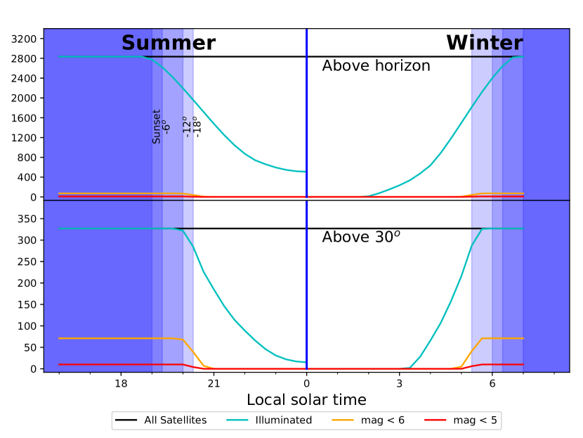
Figure 8: Number of illuminated satellites above the horizon (top panel) and above 30$\degr$ elevation, as a function of the local solar time, for Paranal (latitude $-24\aas@@fstack{\circ}6$), accounting for all the satellites from Table 1. Left is for the summer solstice ($\delta_{\mathrm{Sun}}=+23\aas@@fstack{\circ}4$), and right for the winter solstice ($\delta_{\mathrm{Sun}}=-23\aas@@fstack{\circ}4$). The twilights are indicated with blue shading. The black line marks the total number of satellites above the elevation considered, the blue line those that are illuminated, and the orange and red lines those brighter than magnitude 6 and 5, respectively, using the photometric model described in §2.2.

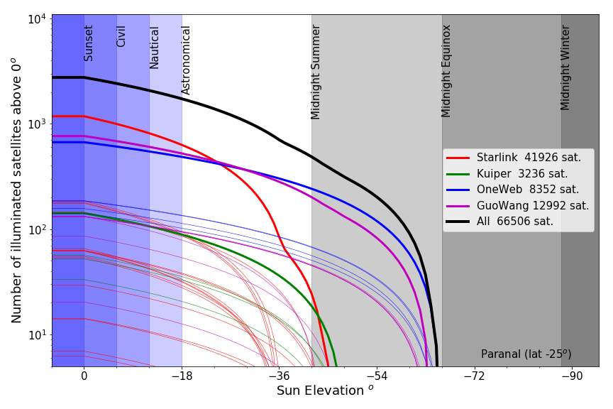
Figure 9: Number of illuminated satellites above the horizon as a function of the Sun elevation, for the constellations listed in Table 1 seen from Paranal (latitude $-24\aas@@fstack{\circ}6$; the dependency with latitude is not strong). The twilights are indicated with blue shadings, and the elevation of the sun at midnight by grey shadings for the solstices and equinoxes. The thin lines represent the individual shells, and the thick lines the totals for each constellation. The upper thick black line is the grand total.

3.2 Spatial fine structure

An outstanding effect of the orbital shells of satellite constellations is the amount of spatial fine structure that arises in the quantity of satellites visible on the local celestial sphere, as illustrated in Fig. 2 and Fig. 4. Of course, first of all we find the effect of the Earth’s shadow, whose behaviour is, as expected, dominated by the diurnal rotation of the planet and by the interplay between observatory latitude and Sun declination. But the structure of satellite shells, combined with orbital mechanics, adds a far from negligible spatial fine structure in the quantity of satellites visible on the local celestial sphere. In particular, as Eqn. 2 shows, each individual shell induces an unavoidable over-density high in the sky over observatories placed at geographic latitudes $\phi$ whose absolute value is close to the orbital inclination $i$. The Northern or Southern boundary of each shell lies along a line on the local celestial sphere that crosses zenith if $\phi=i$, what incidentally happens for Vera Rubin Observatory and some shells currently considered in several constellation designs. These over-densities may coincide with the culmination elevation of some key objects (let us say, for instance, LMC or SMC in the South, or M31 and M33 in the North). Given the inclination $i$ of one orbital shell and the latitude $\phi$ of the observatory, the shell boundary cuts the local meridian at a declination $\delta$ that can be deduced from the following equation (justified in Appendix A.5):

$$\sin{(\delta-\phi)}=\frac{R_{\oplus}+h_{\mathrm{sat}}}{R_{\oplus}}\sin{(\delta-i)}$$ (9)

3.3 Contribution to the sky brightness

a

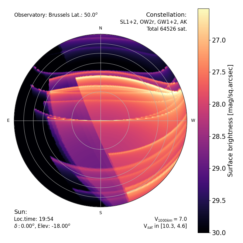
b

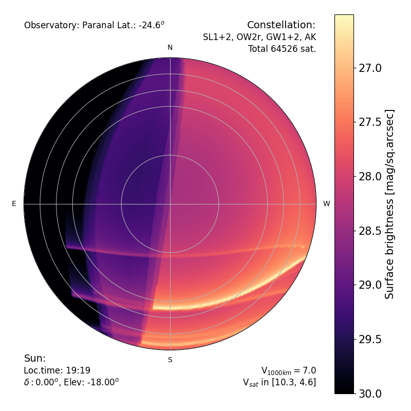
Figure 10: Sky brightness contribution from the satellites (using the constellations from Table 1), at astronomical twilight at latitudes $+50\degr$ (a) and $-25\degr$ (b). Typical sky surface brightness in the visible is 21.7 mag/sq.arcsec or brighter. The satellites used all have $v_{\mathrm{1000km}}=7$, resulting in visual magnitudes in the range indicated at the bottom right corner.

The satellites, including those that are not directly detected, contribute to the sky background. To evaluate this effect, surface brightness maps were computed. The magnitude of a satellite from a constellation was evaluated using Eqn. 6, then converted into flux, and finally used to weight the satellite density map described in §2.1.3. A total flux density map was obtained summing the contributions of all satellite shells, and transformed into surface brightness in mag/sq.arcsec. An example is presented in Fig. 10. In the illuminated part of the shells, the satellites contribute to a surface brightness in the 28–29 mag/sq.arcsec range (0.3–0.7 $\upmu$cd m^-2), with peaks around 26.5 mag/sq.arcsec (2.7 $\upmu$cd m^-2) at the cusps of the constellations. The surface brightness of the dark night sky is around $V=21.7$ (Patat, 2008) (225 $\upmu$cd m^-2), which means that the satellites from Table 1 will contribute at most an additional $\sim 1\%$ to the sky brightness in the worst areas of the sky. The contribution to the sky brightness is therefore small, and the simulations and mitigation focus on the discrete contamination by individual satellites.

Kocifaj et al. (2021) have evaluated the increase in diffuse sky brightness caused by all current space objects with sized between $5\times 10^{-7}$ m to 5 m at altitudes above 200 km. They estimate that this excess is 16.2 $\upmu$cd m^-2 (24.6 mag/sq.arcsec) and can reach 21.1 $\upmu$cd m^-2 (24.3 mag/sq.arcsec)at astronomical twilight, corresponding to about 10% of the natural sky brightness. That excess is dominated by the small objects (mm and below), i.e. space debris. The macroscopic satellites composing the constellations discussed in this paper will not contribute much to the diffuse sky brightness provided they are not ground into microscopic debris.

3.4 Effect on observations

Table 3: Characteristics of instruments and exposures used for the simulations.

Inst. Tel. Obs.	$l$	$D$		Field	$t_{\mathrm{exp}}$ [s]	$r$ [arcsec]	Mag.
Visible and near-IR Imagers
EFOSC NTT ESO (La Silla)	$-29\aas@@fstack{\circ}25$	3.6	Vis	$4\arcmin$	300	1	24.2	Focal reducer (Buzzoni et al., 1984)
FORS VLT ESO (Paranal)	$-24\aas@@fstack{\circ}6$	8.2	Vis	$6\arcmin$	300	0.8	25.2	Focal reducer (Appenzeller et al., 1998)
HAWKI VLT ESO (Paranal)	$-24\aas@@fstack{\circ}6$	8.2	NIR	$7\aas@@fstack{\prime}5$	60	0.6	21.4	Near-IR imager (Kissler-Patig et al., 2008)
MICADO ELT ESO (Armazones)	$-24\aas@@fstack{\circ}6$	39.	NIR	$50\arcsec$	60	0.015	24.9	Visible and near-IR imager with adaptive optics on the ELTa
OmegaCam VST ESO (Paranal)	$-24\aas@@fstack{\circ}6$	2.4	Vis	$1.0\degr$	300	0.8	23.9	Survey wide-field imager (Kuijken et al., 2002)
1.5m Catalina U.AZ (Mt. Lemmon)	$32\aas@@fstack{\circ}4$	1.52	Vis	$2.2\degr$	30	1.5	21.4	Survey wide-field imagerb
LSST Cam. SST VRO (Pachon)	$-30\aas@@fstack{\circ}2$	8	Vis	$3.0\degr$	15	0.8	24.6	Survey wide-field imagerc
0.7m Catalina U.AZ (Mt. Bigelow)	$30\aas@@fstack{\circ}4$	0.7	Vis	$4.4\degr$	30	3	19.8	Survey wide-field imagerb
Photo	$-30\degr$	0.07	Vis	$75\degr\times 55\degr$	60	60	10	Photographic camera with a wide-angle lens from a good site.
Visible and near-IR Spectrographs
FORS VLT ESO (Paranal)	$-24\aas@@fstack{\circ}6$	8.2	Vis	$6\arcmin\times 1\arcsec$	1200	0.8	22.0	Long-slit low-resolution spectrograph (Appenzeller et al., 1998)
UVES VLT ESO (Paranal)	$-24\aas@@fstack{\circ}6$	8.2	Vis	$10\arcsec\times 1\arcsec$	1200	0.8	17.0	High-resolution echelle spectrograph (Dekker et al., 2000)
4MOST-L VISTA ESO (Paranal)	$-24\aas@@fstack{\circ}6$	4	Vis	$4\aas@@fstack{\circ}1$	1200	0.8	20.5	Multi fibre1 spectrograph (low res.) (de Jong et al., 2016)
4MOST-H VISTA ESO (Paranal)	$-24\aas@@fstack{\circ}6$	4	Vis	$4\aas@@fstack{\circ}1$	1200	0.8	18.6	Multi-fibre1 spectrograph (med res.) (de Jong et al., 2016)
ESPRESSO VLT ESO (Paranal)	$-24\aas@@fstack{\circ}6$	8.2	Vis	$0\aas@@fstack{\prime\prime}5$	1200	0.5	15.8	High-resolution echelle (Pepe et al., 2021)
Thermal IR
VISIR VLT	$-24\aas@@fstack{\circ}6$	8.2	ThIR	$60\arcsec$	10	$0\aas@@fstack{\prime\prime}2$	–	Imager (Lagage et al., 2004)
METIS ELT	$-24\aas@@fstack{\circ}6$	39	ThIR	$10\arcsec$	10	$0\aas@@fstack{\prime\prime}03$	–	Adaptive Optics Imager on ELTd,2

$l$: latitude; $D$: diametre of the telescope; Field: field of view of the instrument; $t_{\mathrm{exp}}$: exposure time [s]; $r$: resolution element [arcsec]; Mag: $5\sigma$ limiting magnitude for a point source for an exposure of duration $t_{\mathrm{exp}}$.

References: a, https://elt.eso.org/instrument/MICADO/ - b, https://catalina.lpl.arizona.edu/about/facilities/telescopes - c, https://www.lsst.org/about - d, https://elt.eso.org/instrument/METIS/

Notes: 1: 4MOST is a multi-object spectrograph equipped with 2436 fibres. Monte-Carlo simulations showed that, on average, a satellite crossing the field of view will affect 1.3 fibres. 2: METIS also has a high-resolution spectrograph.

To evaluate in more detail the effects of satellite constellations on observations, we studied a series of representative instruments and telescopes. For each of them, we consider the field of view (size or diameter in case of 2D field, length and width for a slit, diameter of the aperture in case of a fiber), a typical exposure time, and the limiting magnitude (obtained from the Exposure Time Calculators for ESO instruments, documentation or private communications for others). We also estimate the magnitude causing heavy saturation either as 5 mag brighter (i.e. 100 times) than the saturation level or from publications. Table 3 lists the parameters of the exposures and instruments.

a: Trails per exposure
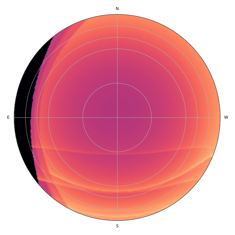
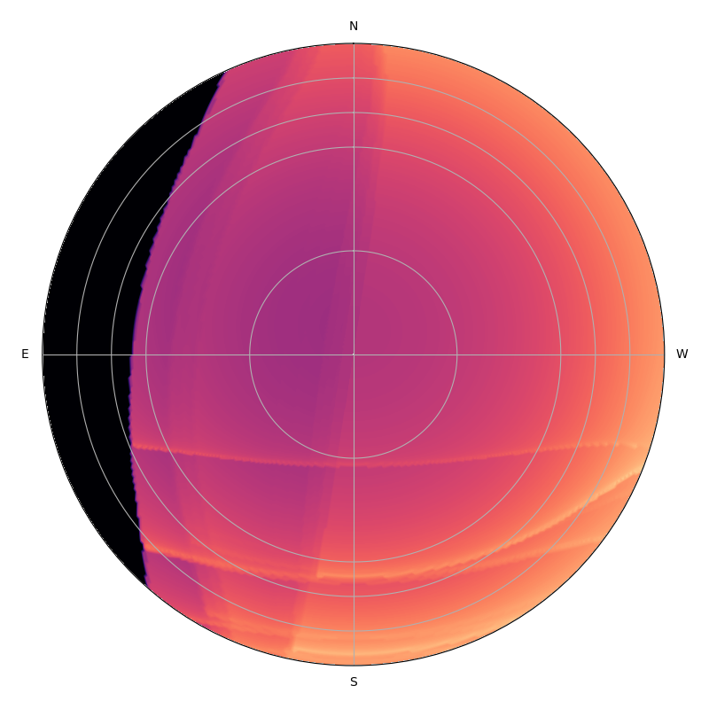
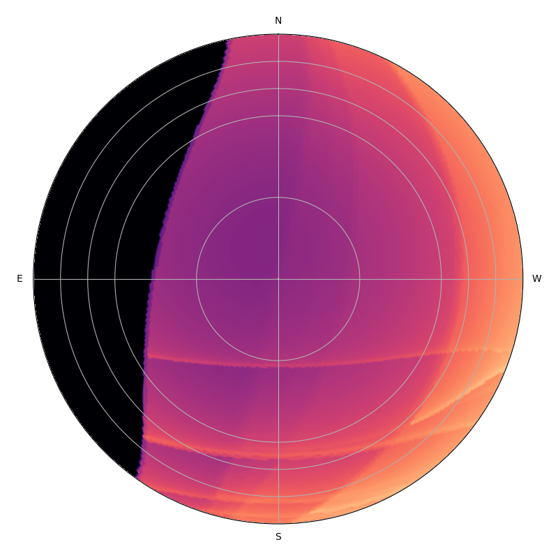
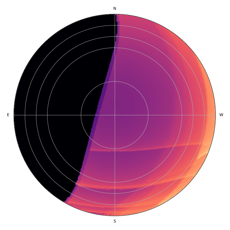
Sun Elevation: $-12\degr$, Average: 0.20 trail	$-18\degr$, 0.16	$-24\degr$, 0.081	$-30\degr$, 0.045
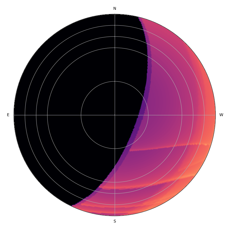
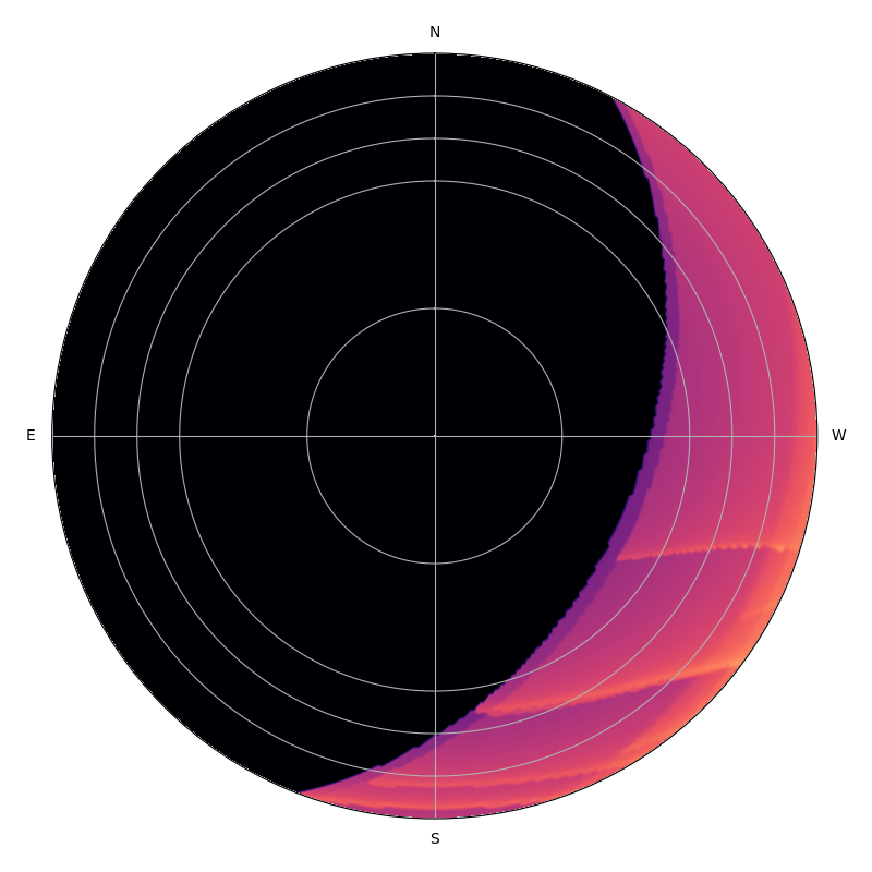
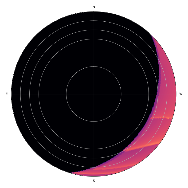
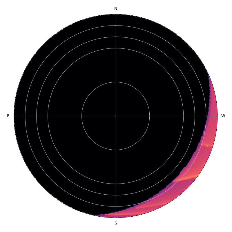
$-36\degr$, 0.023	$-42\degr$, 0.005	$-48\degr$, 0	$-54\degr$, 0
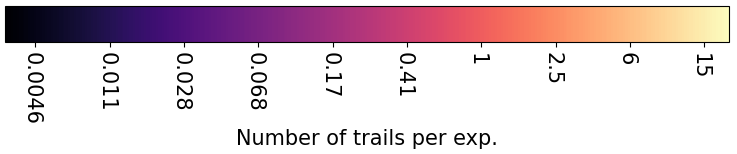
b: Fraction of observations lost to satellite trails
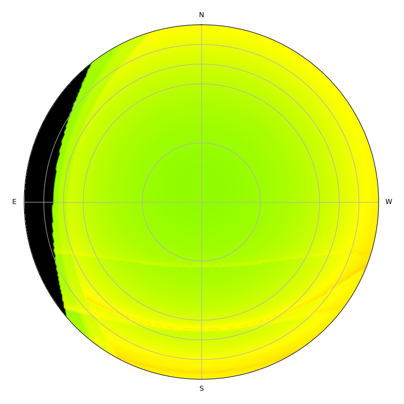
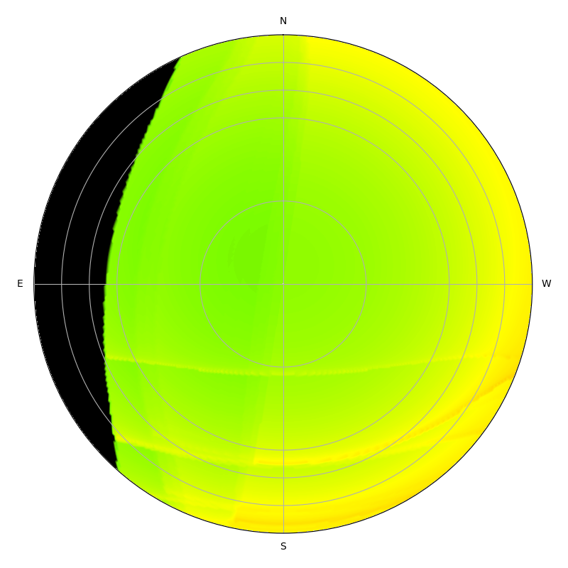
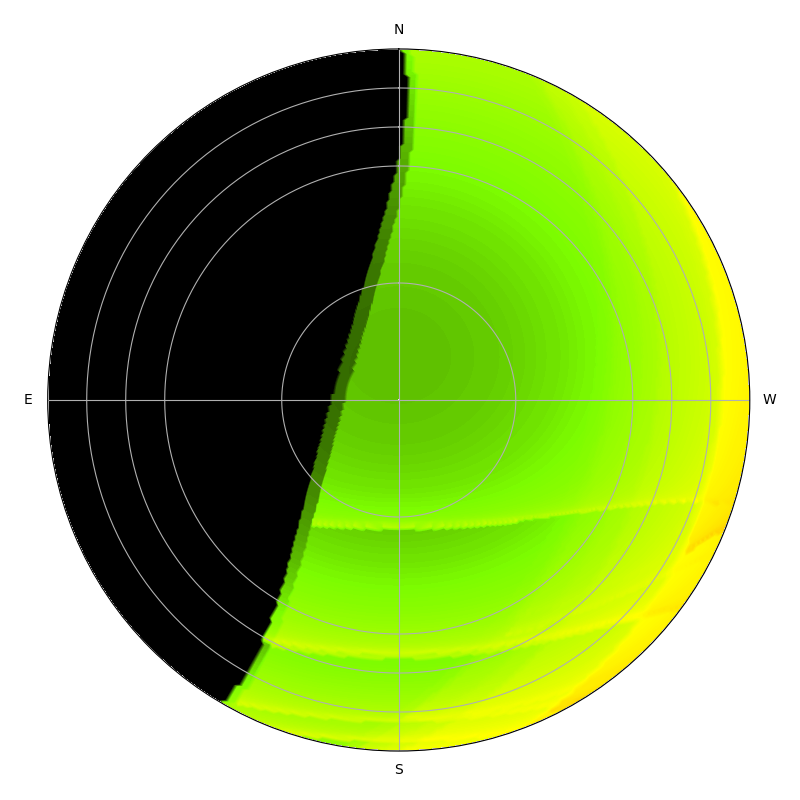
Sun Elevation: $-12\degr$, Average: 0.56%	$-18\degr$, 0.44%	$-24\degr$, 0.23%	$-30\degr$, 0.12%
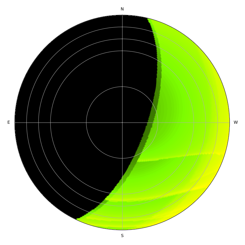
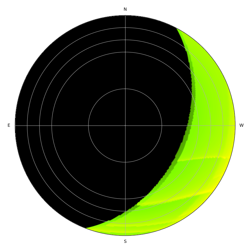
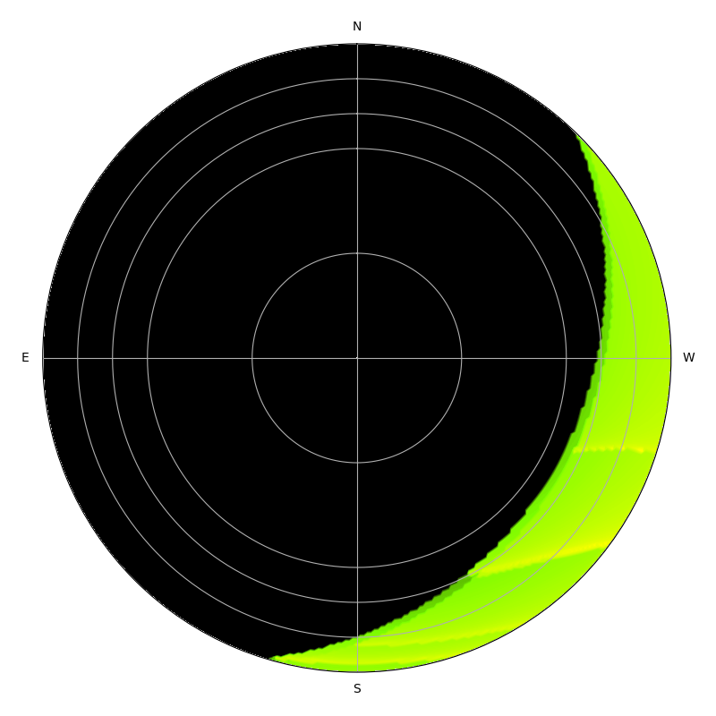
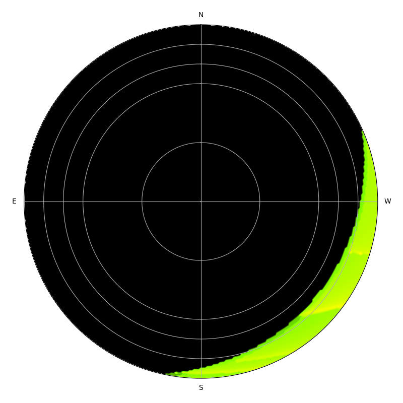
$-36\degr$, 0.06%	$-42\degr$, 0.01%	$-48\degr$, 0%	$-54\degr$, 0%

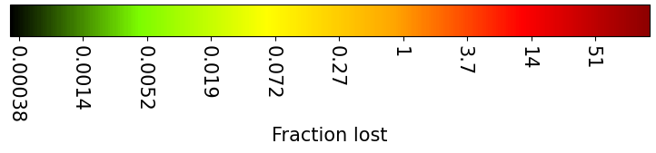
Figure 11: Sky maps of the number of detectable satellite trails (a) and effect on the observations (b), for all the satellites from Table 1 on a FORS2 image ($6\arcmin$ field of view, 5 min exposure time) on Paranal ($-24\aas@@fstack{\circ}6$ latitude) at equinox. The circles indicate elevations $0\degr$, $10\degr$, $30\degr$, and $60\degr$. The legend of each plot gives the Sun elevation and the average number of trails (a) and the losses they cause (b) for observations above $30\degr$ elevation All satellites are brighter than the detection limit, and none is bright enough to cause heavy saturation.

For each constellation shell, the instanteneous satellite density, angular velocity and apparent and effective magnitudes were estimated. The number of trails affecting an exposure was obtained using Eqn. 1, using $A_{\mathrm{fov}}=L_{1}\times L_{2}$ for the field of view (with $L_{1}$ the length and $L_{2}$ the width of the FOV, $L_{1}>L_{2}$) and $L_{\mathrm{fov}}=L_{1}$ in the second term of Eqn. 1 – this maximises the cross-section for trails. $N_{\mathrm{sat}}$ was computed for each shell accounting for the effective magnitude of the satellites in that shell.

a: Imagers
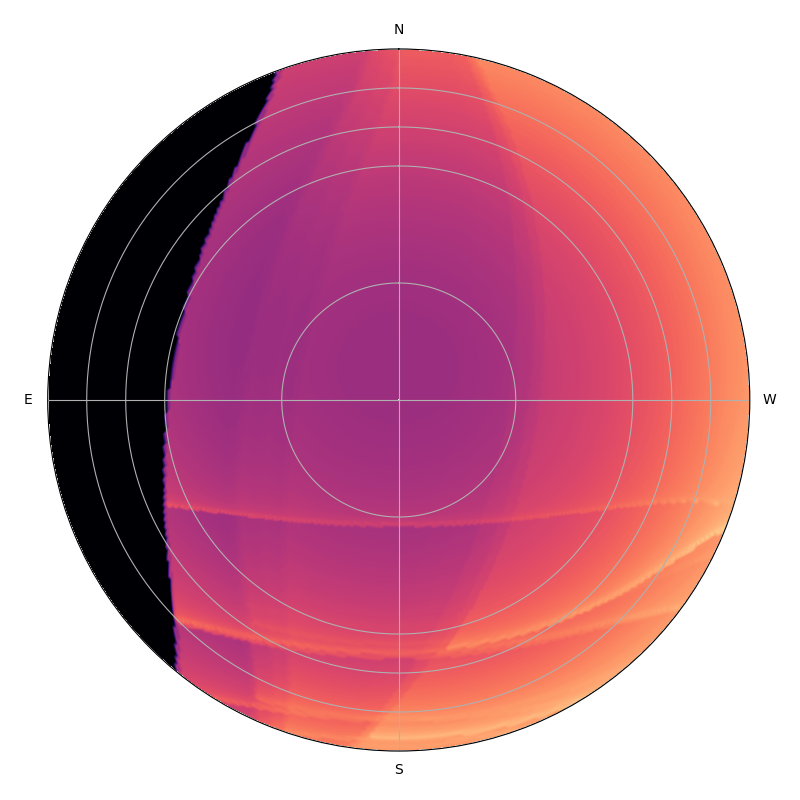
FORS (VLT, ESO, Paranal) 25.2 Average: 0.16 trail, 0.44% loss
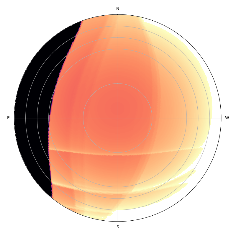
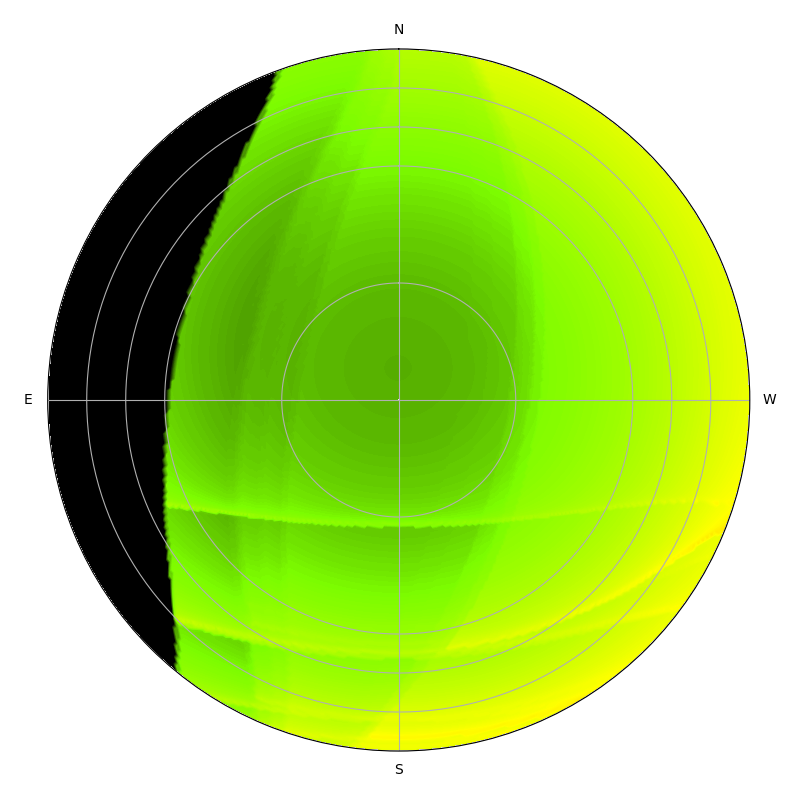
OmegaCam (VST, ESO, Paranal) 23.9, 1.60 trail, 0.22% loss
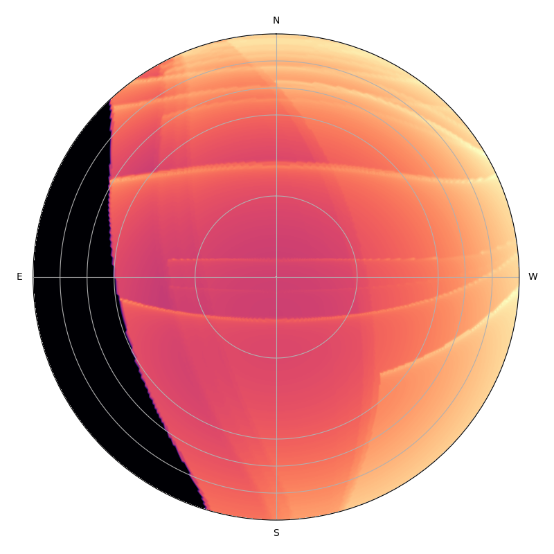
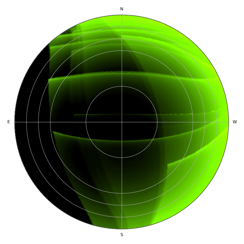
1.5m G96 (Catalina, U.AZ, Mt. Lemmon) 21.4, 0.47 trail, 0.030% loss
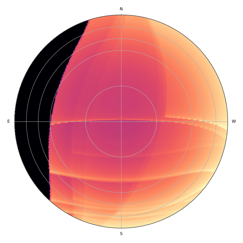
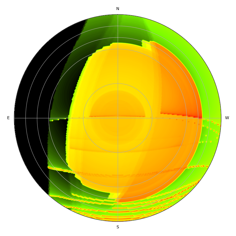
SST Cam. (SST, VRO, Pachon) 21.4, 0.41 trail, 22.0% loss

Figure 12: Sky maps of the number of detectable satellite trails in an exposure (left) and effect on the observations (right) for a series of imagers (see Table 3 for their characteristics). The legend of each plot also lists the average number of trails above $30\degr$ elevation. The Sun declination is $0\degr$, and its elevation $-20\degr$.

b: Spectrographs
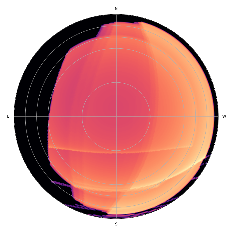
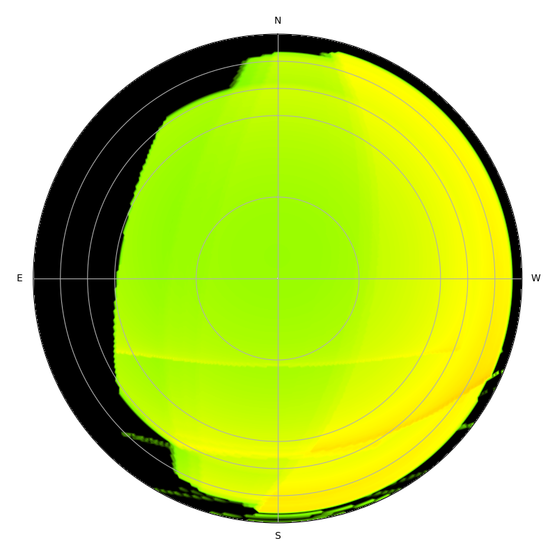
FORS (VLT, ESO, Paranal) 25.2 Average: 0.64 trail, 8.8% loss
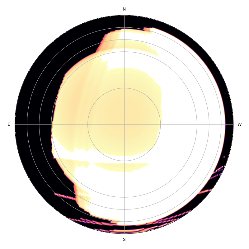
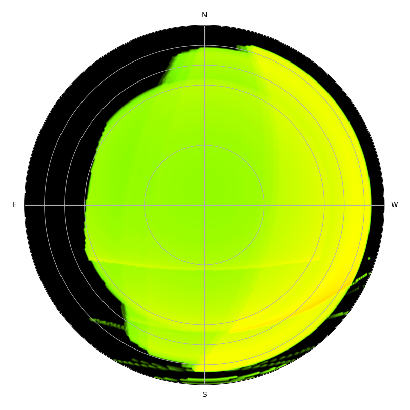
4MOST-LowRes (VISTA, ESO, Paranal), 14.7 trails, 0.78% loss
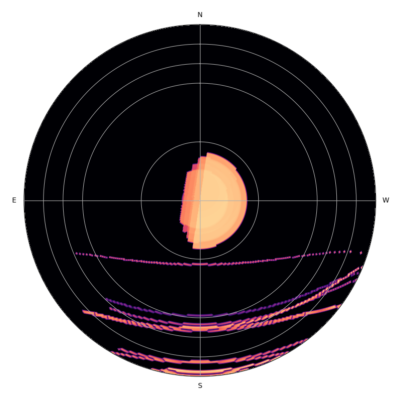
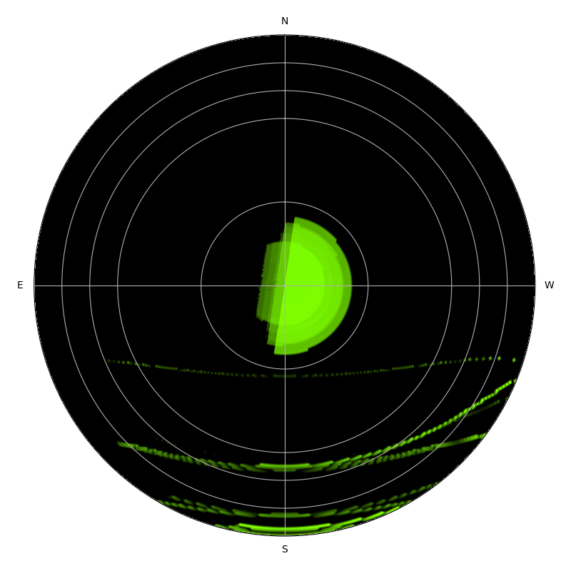
4MOST-HiRes (VISTA, ESO, Paranal), 0.33 trail, 0.018% loss
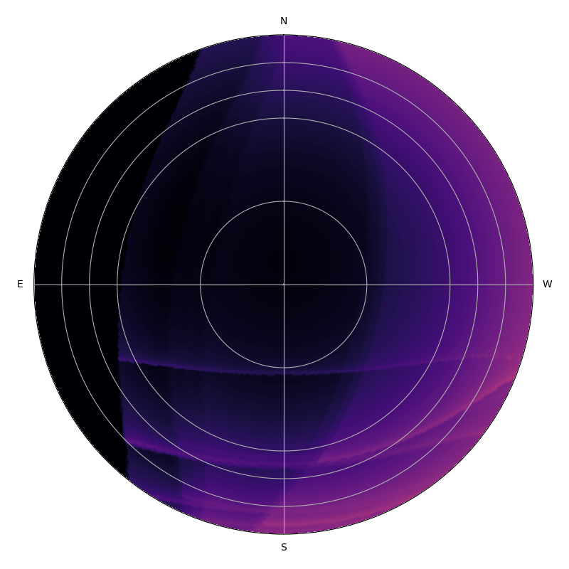
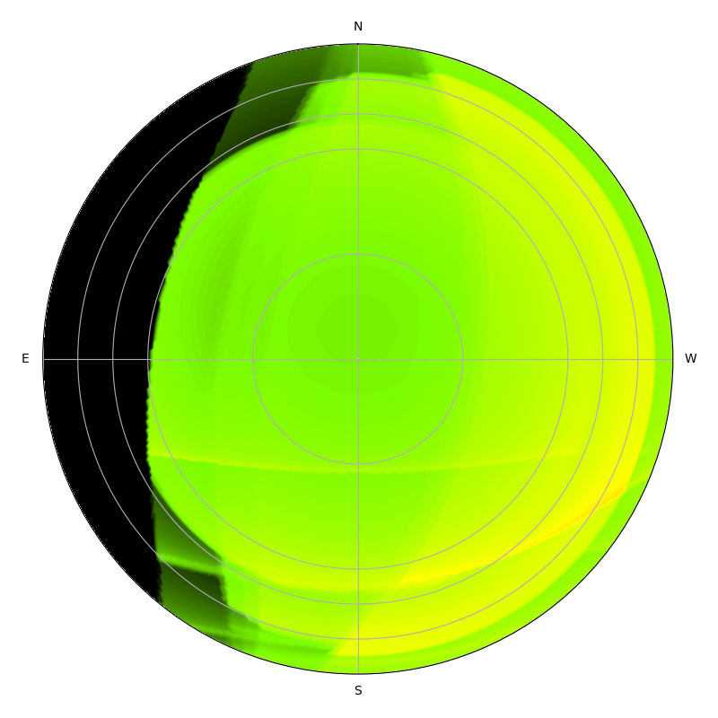
HARMONI (ELT, ESO, Armazones), 0.007 trail, 0.70% loss

Figure 13: Sky maps of the number of detectable satellite trails in an exposure (left) and effect on the observations (right) for a series of spectrographs (see Table 3 for their characteristics). The legend of each plot also lists the average number of trails above $30\degr$ elevation. The Sun declination is $0\degr$, and its elevation $-20\degr$ ($-18\degr$ for 4MOST-HiRes; the values for $-20\degr$ are 0 trail and 0%).

The effect on the observations is computed as follows: Those satellites with an effective magnitude fainter than the $1\sigma$ detection limit were ignored, considering that their trail would be lost in the background noise. Those between the detection limit and heavy saturation limit were counted, and each one was considered to ruin a $5\arcsec$-wide trail across the whole detector. In case of a long slit, they ruin $5\arcsec$ of the slit. In real observations, it is plausible that all or part of the data below a non-saturated trail could be recovered, so this is a pessimistic limit. In the case of a fiber contaminated by a satellite, we consider that the whole spectrum is lost. For trails brighter than the heavy saturation limit, the whole exposure is considered damaged by the charge bleeding and/or electronic and/or optical ghosts. This was repeated for each shell in the constellation, and the effects were summed, resulting in maps of lost fractions. A value of, say, 50% indicates that either 50% of the individual exposures are entirely lost, or that 50% of the pixels in each exposure are lost or, more likely, a combination in between. This was then repeated for several solar elevations ranging from twilight to midnight. Figure 11 displays the resulting sky maps of trail count and fraction lost for an example, with instrument specific all sky plots provided for imagers in Fig. 12 and spectrographs in Fig. 13. The average number of trails per exposure and the average fraction of the exposure lost were computed for the region of the sky above $30\degr$ elevation by integrating the results over that region of the sky. These averages are shown in Fig. 14.

Our software to predict the effect of satellites on observations is available at https://github.com/cbassa/satconsim and can be queried online at https://www.eso.org/~ohainaut/satellites/simulators.html.

a
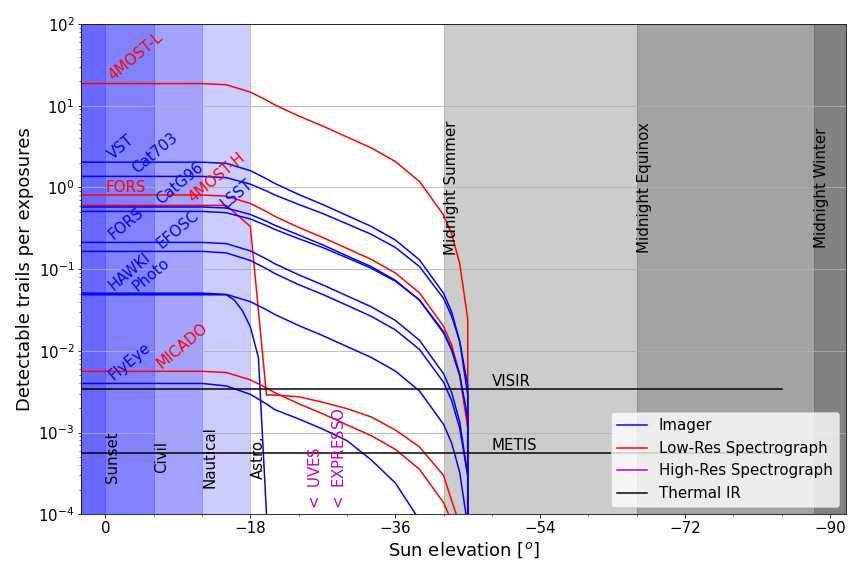
b

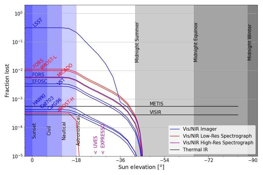
Figure 14: Average number of trails per exposure (a) and average fraction of the exposure lost (b) as a function of the sun elevation, for representative exposures at elevation $>30\degr$ on the instruments listed in Table 3. Twilights are shaded in blue; inaccessible solar elevations are shaded in grey for the equinoxes and solstices for Paranal latitude ($-24\aas@@fstack{\circ}6$).

4 Discussion

As apparent from Fig. 14 and expected from Eqn. 1, the number of trails in an exposure increases with the size $L_{\mathrm{fov}}$ of the field-of-view and with exposure time $t_{\mathrm{exp}}$. The effect of the effective magnitude (Eqn. 7) is less intuitive: for the altitudes of the constellations considered in this study, $m_{\mathrm{1}000km}$ and exposure times, the effective magnitudes fall in the range 13–23, and become fainter as the exposure time increases, with a linear dependency in $t_{\mathrm{exp}}$. As the limiting magnitude for an exposure goes fainter with a dependency in $\sqrt{t_{\mathrm{texp}}}$ (considering the simple sky-noise dominated case) there is, for each instrument, an exposure time beyond which a satellite trail will no longer be detectable. In other words, the contribution from a satellite to the intensity in a resolution element is independent of the exposure time, while the noise increases with $\sqrt{t_{\mathrm{texp}}}$. Overall, the SNR of the satellite trail decreases with $\sqrt{t_{\mathrm{texp}}}$; if an exposure $t_{\mathrm{exp}}$ is immune to satellite trails, longer exposures will also be immune.

Imagers on all but the smallest telescopes typically have a limiting magnitude fainter than the faintest satellite effective magnitude: they are, therefore, affected to some extent by all satellite constellations. For many science cases, the presence of a trail will only result in a loss of useful imaged area (of the order of 0.1 to 1% for a $5\arcsec$ wide trail crossing a $1\degr$ or $8\arcmin$ field of view). There will be, however, some science cases in which even a faint trail will ruin the whole exposure (e.g. photometry of a faint trans-Neptunian object overrun by a satellite), leaving no other choice than repeating the exposure, if this were possible at all (sometimes the repetition is not possible as, for instance, for the photometry of a transient gamma-ray burst). Furthermore, for the most sensitive cameras, some satellites have an effective magnitude brighter than the heavy saturation limit, wreaking havoc in the affected exposures, as on the LSST camera at the Vera Rubin Observatory (VRO), and resulting in much heavier losses (Tyson et al., 2020).

For astrophotography wide-field cameras, the limiting magnitude for satellite trails scales inversely with the focal length of the lens, with every other parameter remaining constant. A wide-angle camera with 30 mm focal length will therefore be 5 mag less sensitive than a 3 m focal length telescope with the same focal ratio. As a consequence, astrophotography will be immune to most satellites in their operational orbits. They can, however, be affected by brighter satellites, e.g. larger satellites, or telecommunication satellites in low altitude transfer orbits (such as the bright strings-of-pearls of 60 very bright satellites, as observed after the early Starlink launches), or specular reflections. Fortunately, these are not numerous: it is foreseen that there will be of the order of 10 trains of satellites around the Earth at any time to replenish the constellations. While potentially spectacularly damaging, these are statistically unlikely and visible only during the brightest parts of twilights.

For spectrographs, the limiting magnitude for a single exposure often falls in the range of the satellites effective magnitudes. As a consequence, those fainter than the limit are not detected and only slightly contribute to the background noise. This is the case for all satellites for high-resolution spectrographs or échelle spectrographs, even on very large telescopes (see the examples of UVES and ESPRESSO on the VLT). However, low- to medium-resolution spectrographs on medium to large telescopes will detect all or many satellites. Furthermore, contrary to imagers, where a satellite leaves a tell-tale trail in the data, slit and fibre spectrographs do not record spatial information. While high-SNR contamination would be easy to notice (e.g. the exposure level is much higher than expected, and the spectral shape does not match that expected for the target), many satellites will leave a signal with a low to moderate SNR. In many cases, the contamination will be at a level comparable to or below that of the science target and therefore unlikely to be detected in real-time. Unless the contamination is flagged using other means (see below, §4.1), there will be cases for which it will become apparent only at the time of the scientific analysis of the spectra. As the contamination will have a solar spectrum, some science cases will be better protected (e.g. study of distant quasars) than others (e.g. study of double stars, where a solar spectrum may not be surprising).

In the thermal IR domain, the overall signal is dominated by the very strong thermal emission from the sky and the telescope. The individual exposure time is therefore kept extremely short (few tens of milliseconds), and the background is registered by chopping (i.e. performing a small position offset by tilting the secondary mirror of the telescope) at about 1 Hz, and nodding (another small offset by moving the whole telescope) every few seconds. In Hainaut & Williams (2020), we conservatively estimated the flux from a satellite at 2000 km at zenith up to 100 Jy in $N$-band (8–13 $\upmu$m) and up to 50 Jy in the $M$ and $Q$-bands (5 and 18-20 $\upmu$m, respectively). The variations between an illuminated and a shadowed satellite are negligible. These fluxes are well above the detection threshold of the thermal IR instruments in Table 3, even accounting for trailing. Because of the extremely short exposure time and small field of view, on average only $6\times 10^{-6}$ trails would be found in a single exposure. However, for most observations, the images are not individually recorded but averaged over a nodding cycle. While the SNR of the trail will be washed away by this average, the values plotted in Fig. 14 correspond to the duration of these averages (10 s). In the case of VISIR on the VLT, it is considered that a satellite ruins a $5\arcsec$ trail across the detector, and for METIS on the larger ELT, the full (smaller) image is ruined by the (broader) trail. Even with these extremely pessimistic assumptions, a negligible fraction of the thermal IR data is affected. For spectroscopy, even at low resolution, the satellite effective fluxes will be below the detection limit.

The case of stellar occultations was discussed in Hainaut & Williams (2020). The effect was found to be small: a 0.02 to 10 millimag for 10 s and 0.1 s exposure time, and extremely improbable: $10^{-4}$ to $10^{-6}$ exposures would be affected. The simulations presented here do not change these estimates. As the eclipse by a satellite would affect only one measurement in a series, even if it could be measured, it would not be similar to the occultation by an exoplanet or a trans-Neptunian object.

The case of visual observations – either naked eye, or through binoculars or telescope – will be considered in a separate paper. In summary, 15 to 50 satellites would be visible in the sky with the naked eye when the sun elevation is between $-12\degr$ and $-24\degr$. When the sun is higher than $-12\degr$, the sky is too bright and no satellite is visible. When the sun is lower than $-24\degr$, no satellite is bright enough to be visible.

4.1 Mitigation

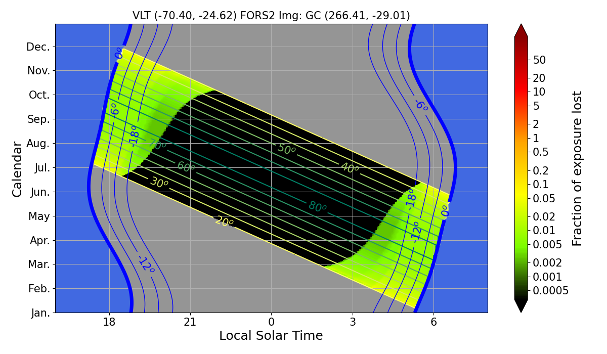
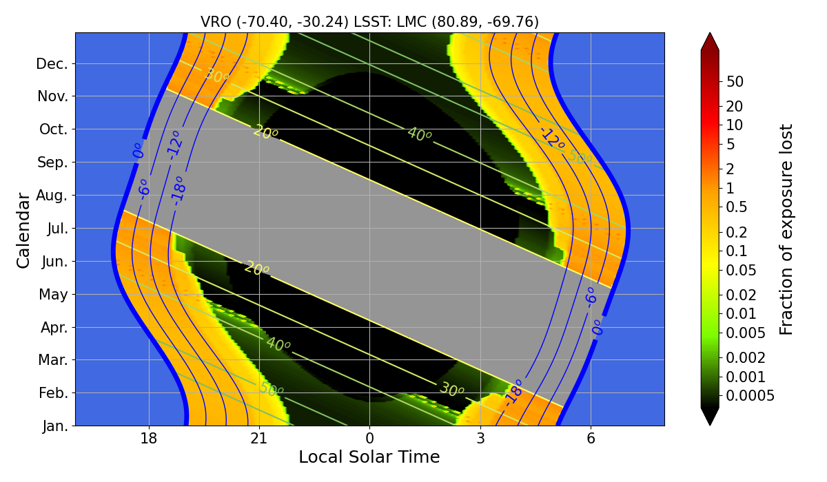
Figure 15: Two examples of calendars showing the visibility of an object from an observatory (Galactic Centre from the VLT, left, and Large Magellanic Cloud from VRO, right). The fraction of observing time lost due to satellites is indicated by the colour scale (1 indicating that all exposures are damaged), for 300 s exposures with FORS2 and 15 s on the LSST camera, respectively. The satellites are the 60+ thousand from Table 1. The blue shading marks daytime, and the blue contours indicate the twilights. The elevation of the object is indicated by the greenish contour lines, and the grey shading indicates the times when the object is below 20$\degr$ elevation.

First order of mitigation refers to the satellites themselves.

Number and altitude: As seen in Fig. 9, the number of illuminated satellites in sight is of course a function of the number of satellites in the constellations, but also of the altitude of the constellation. Furthermore, high-altitude constellations remain illuminated by the Sun much longer than low-altitude ones. The apparent magnitude of a high-altitude satellite will be fainter than that of the same satellite on a lower altitude (Eqn. 6), which is advantageous for small telescopes. However, for large telescopes, the satellite appears extended (Eqn. 8), so that its surface brightness will not decrease much. Overall, a constellation at 1000 km will be more damaging than a three times larger constellation at 500 km altitude.

Brightness of the satellites: Obviously, keeping the brightness of all satellites below the detection limit of all telescopes would be ideal. With the increasing size of the telescopes and sensitivity of the instruments, this is not realistic. An achievable goal would be to reduce the effective cross-section of the satellite so that they remain always below the saturation threshold of the most sensitive instrument. Today and in the foreseeable future, this threshold is set by the SST camera at VRO, at $V_{\mathrm{5}50km}>7$ (Tyson et al., 2020), or $V_{\mathrm{1000\,km}}>8.3$. The changes introduced by SpaceX with VisorSat and modified attitude of the solar array are very promising steps in the right direction: most of the satellites are now below the heavy saturation threshold, while still causing electronic cross talk (Tyson et al., 2020). More systematic measurements of the satellites are needed (as suggested by SatCon1 Recommendation 8, see Walker et al., 2020), and awareness of the satellite operators is a must. SatCon1 Recommendation 5 and Dark & Quiet Skies Recommendation 15 formalize the brightness limit at $V_{\mathrm{550\,km}}>7$.

Once the satellites are in orbit, the next level of mitigation is at the time of preparation and scheduling of the observations. Because of the progression of the Earth shadow through the constellation shells, and of the fine structure in the apparent density of satellites (§3.2), the fraction of losses can change dramatically by pointing the telescope in a slightly different direction. For a given time at a given observatory, sky maps such as those in Fig. 11 would allow an observer to pick objects in the region of the sky that are least affected by satellites. As these maps can be generated on-the-fly, they could be integrated, for instance, in a queue observation optimization algorithm. Another way to consider the scheduling is to pick the best time slots to observe a given object with a specific instrument. Using the same methodology as for the sky maps, a calendar can be populated with the expected density of satellites for an object seen from an observatory. Such calendars, some examples of which are displayed in Fig. 15, could be used when allocating specific telescope time to an observation program in traditional visitor mode. Obviously, both the sky maps and calendars will introduce additional complexity in the scheduling process, and will not resolve all issues. For instance, some observations must be performed at a given time (e.g. an exoplanetary transit observation).

A more aggressive mitigation would be to close the shutter of the instrument just before a damaging satellite enters the field of view, and re-open it just after it left. As the satellites move at apparent speeds of $\sim 0.1$ to $\sim 1\degr$ s^-1, the interruption would be extremely short, virtually nullifying the losses of exposure time. The challenge is to send the signal to the shutter at the right time. Two methods can be envisioned:

The first would rely on a complete, accurate and up-to-date database of orbital elements so that the position of all satellites can be computed at any time, and offending ones identified in times. However, the accuracy of ephemerides, both in position and in timing, must be of the order of the field-of-view. An accuracy of a fraction of a degree (and 1 s) may be achievable, making this viable for imagers. An accuracy of $\sim 1\arcsec$, required for spectrographs, would imply predicting the position of the satellites at 2–5 m accuracy, with a timing precision of $1/100$ s. This method presents various challenges: the database must be complete; it must be up-to-date (as non-keplerian effects, including active orbital corrections, modify the orbit with a time-scale of up to a few days); it must be precise (the current standard Two-Line Elements do not provide the required precision); the computations must be done with the appropriate precision, and scan the whole database for each observation. Furthermore, this method would not work for all instruments: large survey cameras tend to be fairly heavy and slow, precluding rapid and repetitive shutting and opening.

The second method would rely on an auxiliary camera mounted in parallel with the main telescope, with a field of view of 5 to $10\degr$ (a few degrees larger than the field of the main instrument). This camera would take an image of the field about every second, and an analysis system would detect any transient object. An object moving towards the science field of view would trigger the closing of the shutter. The challenge here is to build a system fast enough to process the data in real-time, and a camera sensitive enough to detect the satellites. For instruments sensitive to all the satellites down to the faintest (e.g. imagers on large telescopes), it may not be realistically feasible. However, for spectrographs, which have a brighter limiting magnitude, a 30 cm auxillary telescope with a fast read-out detector is promising. Spectrographs would strongly benefit from this mitigation, as their exposures tend to be much longer than those of imagers (and therefore the loss of an exposure more costly), and because they lack spatial information, what makes it possible that the contamination will remain unnoticed until the data are analysed.

The final stage of mitigation is an a posteriori subtraction of the satellite trail from the data. This also comes with some limitations. Saturated trails (e.g. on a survey camera on a large telescope like the SST Cam at VRO) are un-recoverable. Fainter trails may be identified on images, modelled and subtracted. However, atmospheric scintillation will make these trails irregular, and difficult to model. Even assuming that they can be cleanly subtracted (and that this subtraction is trusted by the scientist), they will result in an increase of the photon noise. It may be safer to mask them and filter them out by combining several exposures of the same field. This is already systematically done for various types of blemishes affecting the images, such as cosmic ray hits and gaps between chips in the detector mosaic, and would result in a well-quantified loss of total exposure time in the affected strips, as already taken into account for detector gaps.

The case of slit or fibre spectroscopy is again more difficult: no tell-tale trail reveals the passage of a satellite, which can only be detected as an additional solar-type spectrum added to the data. A solar spectrum can be iteratively subtracted from the spectrum until the residual shows no hint of the satellite. While this would work for some science cases, it will be more difficult or even impossible in other situations (e.g. a program studying stellar abundances or binary stars).

Finally, the last resort of mitigation consists in repeating the observations that have been damaged by a satellite. In some cases, this will be immediately obvious and easily detected when controlling the quality of the data. In other cases, the effect will be more subtle. Some observations will be simple to re-acquire. Others will be lost forever (a short transient phenomenon, like the optical counterpart of a gravitational wave event).

Overall, no mitigation method will single-handedly work for all instruments and all science cases. Moreover, each of these mitigations comes with a cost that should be carefully compared to the cost of the observing time loss: in many cases, repeating the observation may be cheaper (economically and scientifically) than protecting it.

The way forward is to improve the situation at each step, starting with a collaboration with the satellite operators to make the satellite less bright, continuing with smarter scheduling of the observations, where the work presented in this paper will help thanks to the fast and accurate information it provides, shutter control where possible, and accounting for the inevitable remaining trails in the data.

Appendix A Derivation of key expressions

In the following paragraphs we first show the derivation of Eqn. 2, the probability density function $P(\phi,i,h_{\mathrm{sat}})$ (§A.1). We later get into some geometric details on the relation between the geocentric and topocentric positions of the satellites, impact angle of the line of sight on a shell, and the apparent, observed, angular velocity of satellites (§A.2, §A.3 and §A.4). Finally, in §A.5), we provide some equations on how to locate on the sky the intersection of constellation shell boundaries with the local meridian (Eqn. 9 and some related expressions).

A.1 Probability density

The analytical probability density function $P(\phi,i,h_{\mathrm{sat}})$ displayed in Eqn. 2 is at the core of many of the simulations included in this paper. Let us get into its derivation, down to some degree of detail. We will also prove that its integral is equal to unity.

For a one single satellite in a circular orbit with inclination $i$ and orbital altitude $h_{\mathrm{sat}}$ we first obtain the angle $\beta$ between the orbit and any parallel, as a function of latitude $\phi$. At the nodes the parallel is the equator and we have $\beta=i$. The general situation is depicted in Fig. 16. In that diagram $Q+i=90^{\circ}$ and $Q^{\prime}=90^{\circ}+\beta$. Our problem is finding $Q^{\prime}$ as a function of known quantities. This is solved via the law of sines:

$$\sin 90^{\circ}\sin Q=\sin(90^{\circ}-\phi)\sin Q^{\prime};$$ (10)

$$\sin(90^{\circ}-i)=\sin(90^{\circ}-\phi)\sin(90^{\circ}+\beta);$$ (11)

$$\cos\beta=\frac{\cos i}{\cos\phi}.$$ (12)

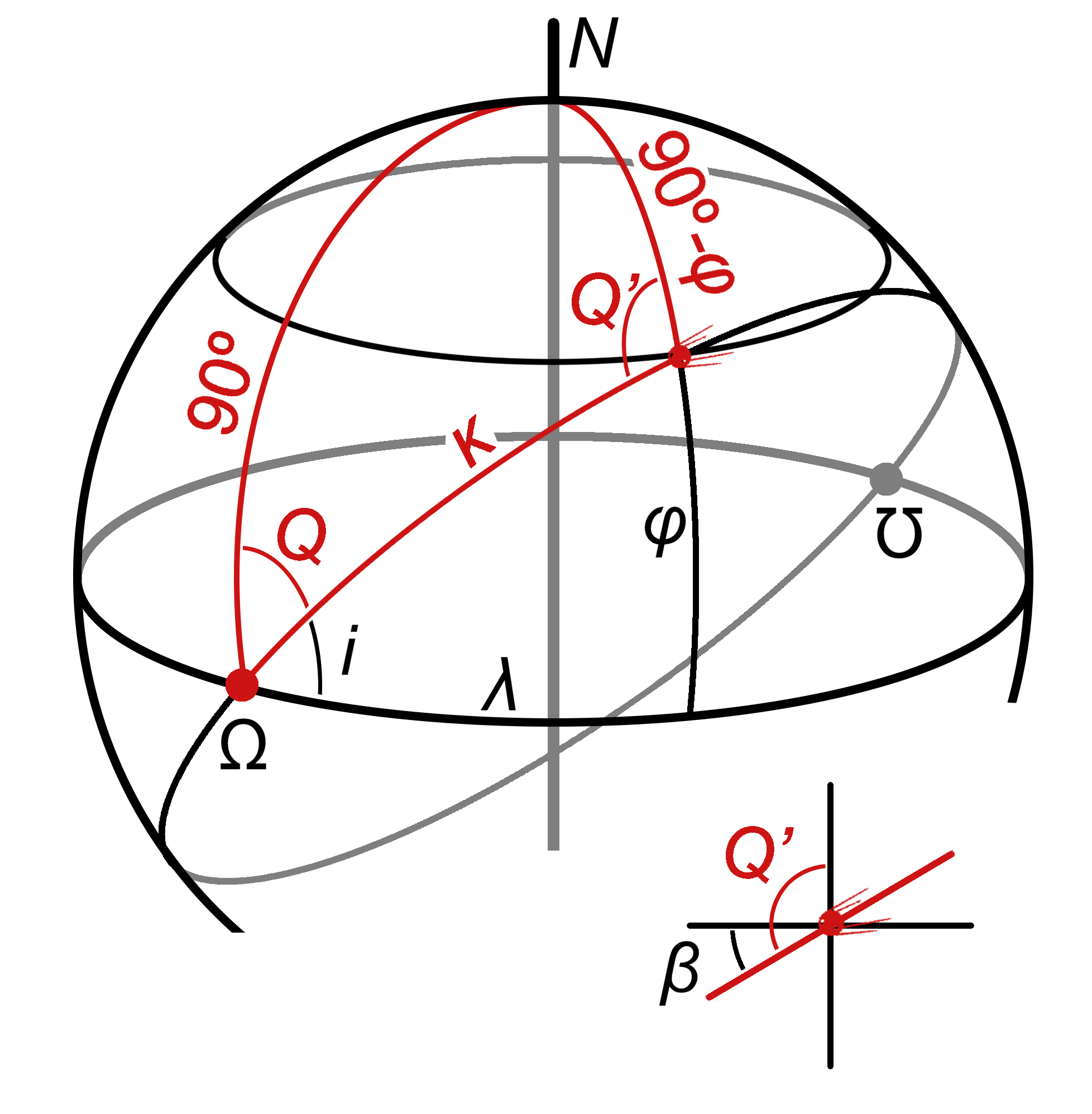
Figure 16: The spherical triangle to obtain the angle $\beta$ between the orbit and the parallel of latitude $\phi$. Angle $\kappa$ indicates the longitude of the satellite measured from the ascending node along its orbit. With $\lambda$ we indicate the difference between the longitude of the satellite and that of the ascending node.

The only satellite inside our orbit induces a linear density of satellites per angular unit along the orbit itself that is $\Lambda=1/(2\pi)$. We have assumed that the satellite is uniformly distributed in time along its trajectory, what is true if the orbit is circular. Now we have to transform this angular linear density (satellites per unit angle along the orbit) into an angular surface density (satellites per unit solid angle on the orbital shell).

It is worth noting that one single orbit, even considering that its only satellite is uniformly distributed along it with linear density $\Lambda$, in rigour will not induce an uniform surface density over the shell nor in longitude nor in latitude. In longitude, the density will be higher around the nodes and lower at the longitudes corresponding to extreme latitudinal excursions (at $90\degr$ from any node). In latitude we have more or less the opposite: the latitudinal density will be higher where the orbit is tangent to parallels (extreme latitude excursions) and lower at the equator. In any case, it is clear that the density will be zero outside the range $-i<\phi<i$.

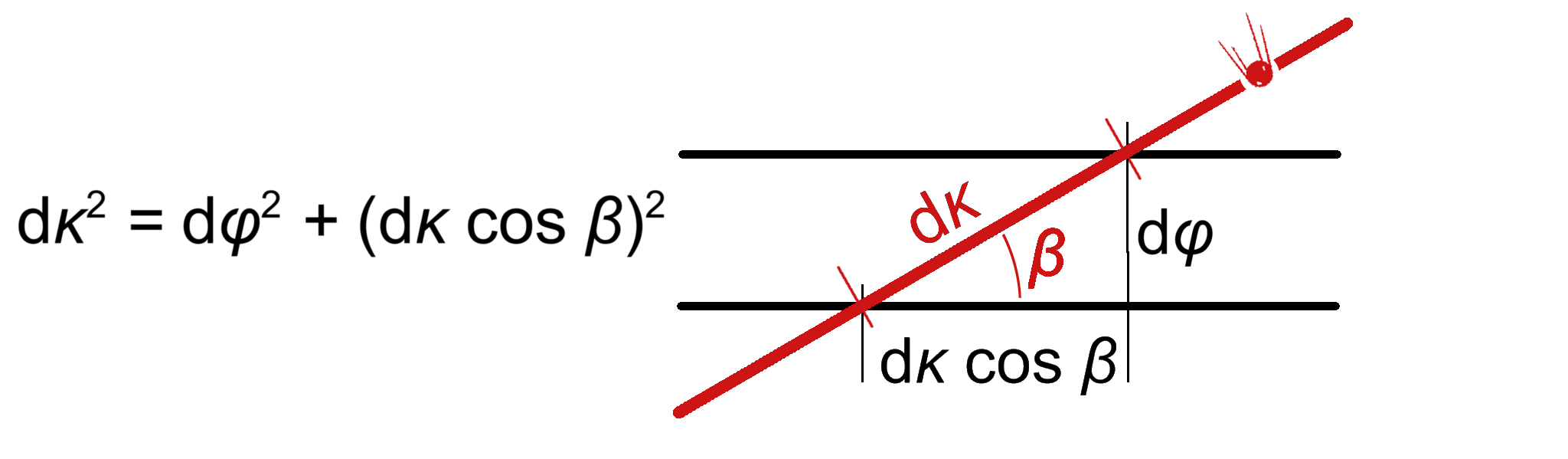
Figure 17: From angular linear density to angular latitudinal density.

However, heterogeneity of density in longitude is not important to our purposes, because it will smooth out after many iterations, due to the Earth rotation and to random initialization conditions. Also, in normal cases we will have many satellites inside the same orbit and many similar orbits inside one shell (with different longitudes of the ascending node), in such a way that the smoothing in longitude will be very efficient and fast. So, we assume, and impose, that the final density distribution has to have cylindrical symmetry and we can concentrate on the latitudinal behaviour.

Let us depict a latitude band of infinitesimal angular width d$\phi$ at latitude $\phi$, as shown in Fig. 17. The arc of the orbit span crossing the band is d$\kappa$ and this relation holds:

$$\mathrm{d}\kappa^{2}=\mathrm{d}\phi^{2}+(\mathrm{d}\kappa\cos\beta)^{2}.$$ (13)

Then:

$$\mathrm{d}\kappa^{2}=\frac{\mathrm{d}\phi^{2}}{1-\cos^{2}\beta}\leavevmode\nobreak\ \Rightarrow\leavevmode\nobreak\ \mathrm{d}\kappa=\frac{\mathrm{d}\phi}{\sin\beta}.$$ (14)

Introducing density $\Lambda$ to pass from arc $\kappa$ to satellites per unit arc in latitude $p=\Lambda\kappa$:

$$\mathrm{d}p=\Lambda\mathrm{d}l=\Lambda\frac{\mathrm{d}\phi}{\sin\beta}=\frac{\mathrm{d}\phi}{2\pi\sin\beta}.$$ (15)

Next, we obtain the expression for the latitudinal angular probability density due to one single orbit with one single satellite:

$$\frac{\mathrm{d}p}{\mathrm{d}\phi}=\frac{1}{2\pi\sin\beta}=\frac{1}{2\pi\sqrt{1-\cos^{2}\beta}}.$$ (16)

But, as shown in Eqn. 12, $\cos\beta=\cos i/\cos\phi$ and, thus:

$$\frac{\mathrm{d}p}{\mathrm{d}\phi}=\frac{\cos\phi}{2\pi\sqrt{\cos^{2}\phi-\cos^{2}i}}.$$ (17)

Note that this density takes into account only one side of the orbit, but each parallel is crossed twice by the same orbit, so that the final true latitudinal angular density is twice this value, $p_{2}=2p$:

$$\frac{\mathrm{d}p_{2}}{\mathrm{d}\phi}=\frac{\cos\phi}{\pi\sqrt{\cos^{2}\phi-\cos^{2}i}}.$$ (18)

This latitudinal angular density would be measured in fractions of the sample per unit angle in latitude. We now divide by the length of a parallel at latitude $\phi$, $2\pi\cos\phi$, to transform this angular latitudinal density into true density per unit solid angle, and label the resulting probability density function as $c(\phi,i)$:

$$c(\phi,i)=\frac{\mathrm{d}p_{2}}{\mathrm{d}\Omega}=\frac{1}{2\pi^{2}\sqrt{\cos^{2}\phi-\cos^{2}i}}.$$ (19)

This density per unit solid angle can be converted into the true, physical surface density, in units of fractions of the sample per surface unit on the shell, by dividing by the radius of the shell squared, $(R_{\oplus}+h_{\mathrm{sat}})^{2}$. Also, by using that $\cos^{2}\phi-\cos^{2}i=\sin^{2}i-\sin^{2}\phi$, and that both expressions are differences of squares, we end up with four equivalent formulations of our probability surface density function:

$$P(\phi,i,h_{\mathrm{sat}})=\frac{\mathrm{d}p_{2}}{\mathrm{d}S}=\frac{1}{(R_{\oplus}+h_{\mathrm{sat}})^{2}}\frac{\mathrm{d}p_{2}}{\mathrm{d}\Omega}$$ (20)

$$=\frac{1}{2\pi^{2}(R_{\oplus}+h_{\mathrm{sat}})^{2}\sqrt{\cos^{2}\phi-\cos^{2}i}}$$ (21)

$$=\frac{1}{2\pi^{2}(R_{\oplus}+h_{\mathrm{sat}})^{2}\sqrt{(\cos\phi+\cos i)(\cos\phi-\cos i)}}$$ (22)

$$=\frac{1}{2\pi^{2}(R_{\oplus}+h_{\mathrm{sat}})^{2}\sqrt{\sin^{2}i-\sin^{2}\phi}}$$ (23)

$$=\frac{1}{2\pi^{2}(R_{\oplus}+h_{\mathrm{sat}})^{2}\sqrt{(\sin i+\sin\phi)(\sin i-\sin\phi)}}.$$ (24)

Of the four options, we have elected using the last one.

$P(\phi,i,h_{\mathrm{sat}})$ is a probability density distribution and its integral over the space occupied by the sample is unity, as stated in the main text of this article. This may be shown from any of the four forms of the function, but is easier from the first one, Eqn. 21. Noting $R_{\mathrm{sat}}=R_{\oplus}+h_{\mathrm{sat}}$, we have:

$$\int_{\mathrm{shell}}\frac{{\mathrm{d}}S}{2\pi^{2}R_{\mathrm{sat}}^{2}\sqrt{\cos^{2}\phi-\cos^{2}i}}$$ (25)

$$=\int_{\theta=0}^{\theta=2\pi}\int_{\phi=-i}^{\phi=+i}\frac{R_{\mathrm{sat}}^{2}\cos\phi\,{\mathrm{d}}\phi\,\mathrm{d}\theta}{2\pi^{2}R_{\mathrm{sat}}^{2}\sqrt{\cos^{2}\phi-\cos^{2}i}}$$ (26)

$$=\frac{1}{\pi}\int_{-i}^{+i}\frac{\cos\phi\,\,\mathrm{d}\phi}{\sqrt{\cos^{2}\phi-\cos^{2}i}}\leavevmode\nobreak\ .$$ (27)

This last integral is reduced to a straightforward arcsine with the variable change $x=\sin\phi$:

$$\frac{1}{\pi}\int_{x=-\sin i}^{x=\sin i}\frac{\mathrm{d}x}{\sqrt{\sin^{2}i-x^{2}}}=\frac{1}{\pi}\left[\arcsin{\frac{x}{\sin i}}\right]_{-\sin i}^{\sin i}=1.$$ (28)

A.2 Geocentric and topocentric position of the satellites

The number of trails affecting an exposure, given by Eqn. 1 in §2.1.2, relies on the apparent angular velocity of the satellites at that position in the sky.

To compute that velocity, we first have to relate the geocentric longitude and latitude of the satellite ($\theta$, and $\phi$) to the topocentric position vector of a satellite (pointing direction of the telescope, given by $\@vec{OS}$), which is characterized by its right ascension (more precisely, the hour angle) and declination, or equivalently by its azimuth and elevation.

Writing the vectorial relation between the centre of Earth C, the observer O and the satellite S,

$$\@vec{CS}=\@vec{CO}+\@vec{OS}\leavevmode\nobreak\ ,$$ (29)

in geocentric rectangular coordinates ($x$ equatorial at the meridian of the observer, $z$ to the pole, and $y$ completing the referential) using the longitude and latitude of the observer ($\theta_{\mathrm{o}}$, $\phi_{\mathrm{o}}$) and of the satellite ($\theta$, $\phi$), Eqn. 29 becomes

$$R_{\mathrm{sat}}\cos\theta\cos\phi=dx_{OS}+R_{\oplus}\cos\phi_{\mathrm{o}}$$ (30)

$$R_{\mathrm{sat}}\sin\theta\cos\phi=dy_{OS}$$ (31)

$$R_{\mathrm{sat}}\sin\phi=dz_{OS}+R_{\oplus}\sin\phi_{\mathrm{o}},$$ (32)

where $R_{\oplus}$ is the radius of the Earth, $R_{\mathrm{sat}}=R_{\oplus}+h_{\mathrm{sat}}$ is the radius of the satellite orbit, $d=|OS|$, and $(x_{OS},y_{OS},z_{OS})$ the unit vector so that $\@vec{OS}=d(x_{OS},y_{OS},z_{OS})$. The coordinates are obtained from the hour angle and declination of the satellite. We eliminate $\theta$ and $\phi$ by summing quadratically these three equations:

$$d^{2}+2R_{\oplus}(x\cos\phi_{\mathrm{o}}+z\sin\phi_{\mathrm{o}})d-(h_{\mathrm{sat}}^{2}+2R_{\oplus}h_{\mathrm{sat}})=0\leavevmode\nobreak\ .$$ (33)

Solving this quadratic equation leads to two solutions for $d$. The positive one is the distance to the satellite (the negative one is the distance to the satellite shell in the opposite direction, below ground).

Once $d$ is computed, Eqn. 32 can be solved for $\phi$, and then Eqn. 30 and 31 for $\theta$. We have now the geocentric longitude and latitude ($\theta$, and $\phi$) of the satellite that corresponds to a specific, topocentric pointing direction on the local sky.

A.3 Impact angle of the line of sight with the shell

This is the angle $\alpha$ between the line of sight and the normal to the shell, i.e. the angle $\widehat{CSO}$. From the cosine law in triangle CSO, we have:

$$\cos\alpha=\frac{R_{\mathrm{sat}}^{2}+d^{2}-R_{\oplus}^{2}}{2dR_{\mathrm{sat}}}\leavevmode\nobreak\ .$$ (34)

A.4 Apparent angular velocity

A satellite observed in a given detection may either be on the north-bound half of its orbit, or on the south-bound half. Considering the right spherical triangle including the satellite, the ascending node of its orbit and the equator (see Fig. 16), we obtain the longitude difference $\lambda$ between the longitude of the satellite and that of the ascending nodes from:

$$\sin\lambda=\frac{\tan\phi}{\tan i}\leavevmode\nobreak\ ,$$ (35)

from which we get the longitudes of the ascending nodes for both possible orbits:

$$\Omega_{\mathrm{N}}=\theta-\lambda\leavevmode\nobreak\ ,$$ (36)

$$\Omega_{\mathrm{S}}=\theta+\lambda+\pi.$$ (37)

The geocentric velocity vector of a satellite is obtained from:

$$\@vec{v}_{\mathrm{sat}}=v\leavevmode\nobreak\ \@vec{N}\times\@vec{OS},$$ (38)

where $v$ is obtained from elementary celestial mechanics as $v=\sqrt{GM_{\oplus}/R_{\mathrm{sat}}}$, $\@vec{N}$ is the unit vector normal to the orbit (built from the longitude of the ascending node and $i$), $\@vec{N}=\@vec{CS}/|CS|$ is the unit vector pointing from the centre of the Earth to the satellite and $\times$ marks the cross product. This is repeated for both $\Omega_{\mathrm{N}}$ and $\Omega_{\mathrm{S}}$.

The topocentric velocity vectors are obtained by subtracting the geocentric velocity vector of the observer from that of the satellite. The components of these vectors perpendicular to the line of sight OS are the two apparent angular speeds $\omega_{\mathrm{N}}$ and $\omega_{\mathrm{S}}$.

A.5 Declination of the constellation edges

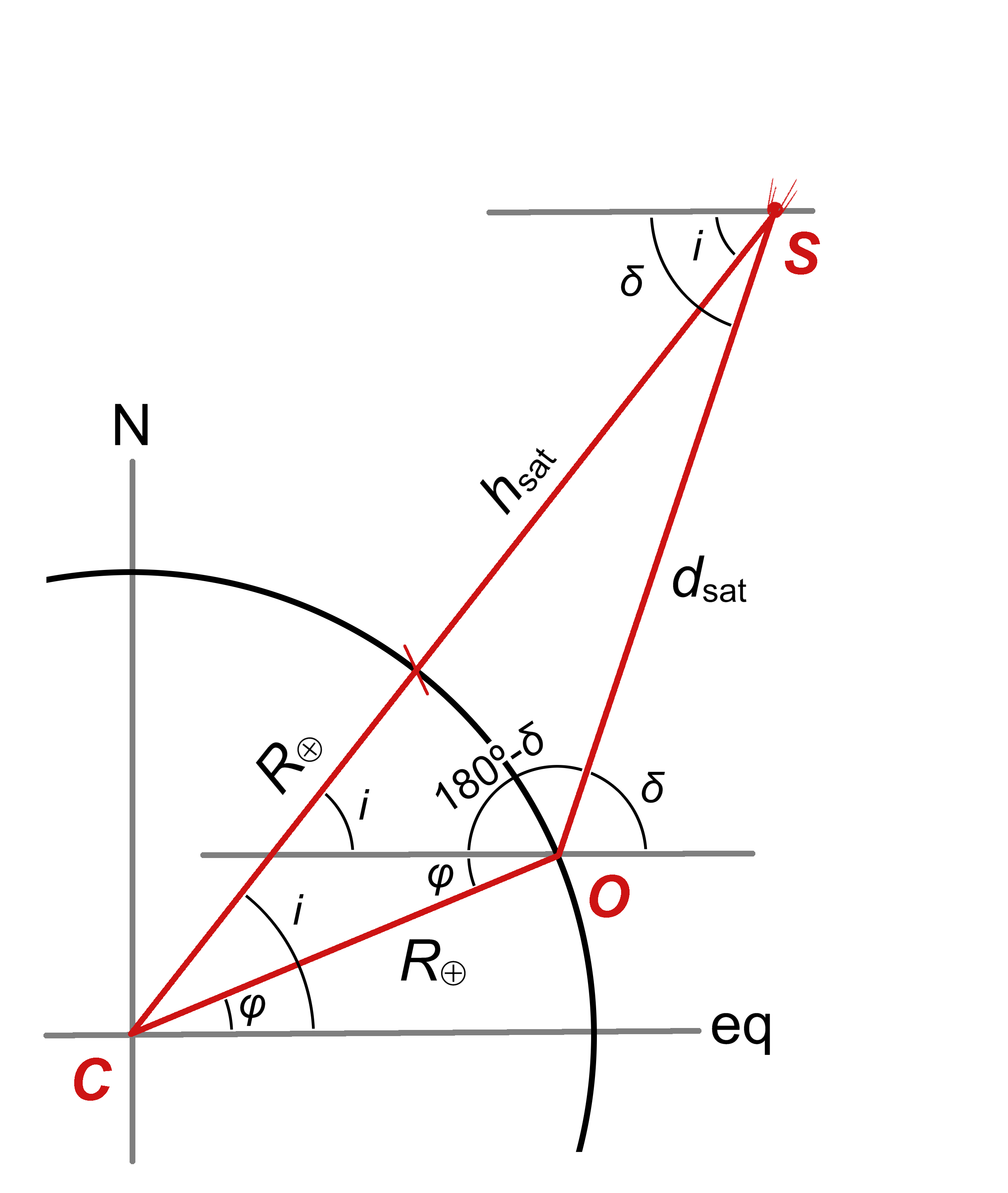
Figure 18: Geometry of shell boundaries at the local meridian. C: Earth centre. O: Observatory. S: Intersection of the northern shell boundary with the local meridian.

Equation 9 relates observatory latitude $\phi$ and shell inclination $i$ to the declination $\delta$ at which the shell boundary cuts the local meridian. It is deduced from elementary geometry (plane sinus theorem) applied to triangle COS in Fig. 18:

$$\frac{\sin[180^{\circ}+(\phi-\delta)]}{R_{\oplus}+h_{\mathrm{sat}}}=\frac{\sin(\delta-i)}{R_{\oplus}}\Rightarrow$$ (39)

$$\sin{(\delta-\phi)}=\frac{R_{\oplus}+h_{\mathrm{sat}}}{R_{\oplus}}\sin{(\delta-i)}.$$ (40)

The same elementary procedure applied to other combinations of sides and angles of triangle COS leads to two additional relations:

$$\sin(\delta-\phi)=\frac{R_{\oplus}+h_{\mathrm{sat}}}{d_{\mathrm{sat}}}\sin(i-\phi)$$ (41)

$$\sin(\delta-i)=\frac{R_{\oplus}}{d_{\mathrm{sat}}}\sin(i-\phi).$$ (42)

To use these two relations it is necessary to introduce the distance $d_{\mathrm{sat}}$ from the observatory to the shell boundary at the meridian, that is also easily deduced from Fig 18 through the plane cosinus theorem:

$$d_{\mathrm{sat}}^{2}=2R_{\oplus}\left(R_{\oplus}+h_{\mathrm{sat}}\right)\left[1-\cos\left(i-\phi\right)\right]+h_{\mathrm{sat}}^{2}.$$ (43)

Appendix B Index of symbols

This is a list of the symbols used in this paper, together with a short definition.

• $\alpha$: impact angle between the line-of-sight and the spherical shell at the satellite

• $\alpha_{\odot}$: solar phase angle, angle Sun-Satellite-observer

• $\chi$: airmass

• $\delta$: declination angle

• $\delta_{\mathrm{sat}}$: density of satellites in a field of view, in satellites per unit solid angle (n/sq.deg).

• $\delta_{\mathrm{trail}}$: density of satellite trails crossing a the field of view, in satellite per linear degree per unit of time (deg^-1 s^-1)

• $\kappa$: angular coordinate of the satellite measured along its orbit, from the ascending node (sometimes called phase in engineering, but we have avoided that denomination to prevent confusions with what we normally understand by phase angle

• $\Lambda$: linear density of satellites per unit angle along the orbit

• $\lambda$: difference of longitudes of the satellite and the ascending node of its orbit (longitude of the satellite measured from the ascending node)

• $\omega_{\mathrm{sat}}$: apparent angular velocity of the satellite as seen by the observer

• $\rho(\phi,i,h_{\mathrm{sat}})=N_{\mathrm{sat}}b$: density of satellites at latitude $\phi$

• $\theta,\phi$: geocentric longitude and latitude of the satellite

• $P(\phi,i,h_{\mathrm{sat}})$: probability density function of finding a satellite (with $i,h_{\mathrm{sat}}$) at latitude $\phi$

• $d$, $d_{\mathrm{sat}}$: distance between the observer and the satellite

• $d_{\mathrm{sat}\odot}$: distance from the Sun to the satellite, $\sim 1$ AU

• $h_{\mathrm{sat}}$: Altitude of the satellites’ orbit, km

• $i$: orbital inclination of the satellites’ orbit, degrees

• $k$: atmospheric extinction coefficient, mag/airmass

• $L_{\mathrm{fov}}$: diameter of the (circular) field of view, degrees

• $l$: latitude of the observer

• $m_{\mathrm{1000km}}$, $m_{\mathrm{500km}}$: zenithal magnitude of the satellite normalized to a distance $d_{\mathrm{sat}}=1000$ km, 500 km

• $m_{\mathrm{eff}}$: effective magnitude of the satellite: the magnitude of a static, point-like object that, during the exposure time considered, would produce the same accumulated intensity in a resolution element than the satellite crossing over a resolution element

• $m_{\mathrm{sat}}$: (visual) magnitude of the satellite

• $m_{\odot}$: magnitude of the Sun

• $n_{\mathrm{1}}$: number of satellites in a single orbital plane

• $n_{\mathrm{plane}}$: number of orbital planes in the constellation shell

• $n_{\mathrm{sat}}$: number of satellites present in the field of view

• $n_{\mathrm{trail}}$: number of satellite trails crossing the field of view during the exposure

• $N_{\mathrm{sat}}$: total number of satellites in the constellation shell

• $p$: geometric albedo of the satellite

• $p(S)$: probability of finding a satellite in region $S$

• $r$: angular size in the plane of sky of a detector’s resolution element or pixel

• $R_{\oplus}$: radius of the spherical Earth,

• $R_{\mathrm{sat}}$: radius of the (spherical) satellite or, in other contexts, radius of the (circular) orbit of a satellite

• $t_{\mathrm{exp}}$: exposure time, in seconds

• $t_{\mathrm{eff}}$: effective exposure time for a satellite, the duration it takes the satellite to cross a resolution element of the detector