Statistical Inference for Linear Mediation Models with High-dimensional Mediators and Application to Studying Stock Reaction to COVID-19 Pandemic
Abstract
Mediation analysis draws increasing attention in many scientific areas such as genomics, epidemiology and finance. In this paper, we propose new statistical inference procedures for high dimensional mediation models, in which both the outcome model and the mediator model are linear with high dimensional mediators. Traditional procedures for mediation analysis cannot be used to make statistical inference for high dimensional linear mediation models due to high-dimensionality of the mediators. We propose an estimation procedure for the indirect effects of the models via a partial penalized least squares method, and further establish its theoretical properties. We further develop a partial penalized Wald test on the indirect effects, and prove that the proposed test has a limiting null distribution. We also propose an -type test for direct effects and show that the proposed test asymptotically follows a -distribution under null hypothesis and a noncentral -distribution under local alternatives. Monte Carlo simulations are conducted to examine the finite sample performance of the proposed tests and compare their performance with existing ones. We further apply the newly proposed statistical inference procedures to study stock reaction to COVID-19 pandemic via an empirical analysis of studying the mediation effects of financial metrics that bridge company’s sector and stock return.
JEL classification: C12; C13
Keywords Mediation Analysis; Penalized Least Squares; Sparsity; Wald test.
1 Introduction
Since the seminal work of Baron & Kenny (1986), mediation analysis has been used in various scientific research, such as economics, psychology, pedagogy, and behavioral science (Conti et al., 2016; Chernozhukov et al., 2021; Mackinnon, 2008; Hayes, 2013; Vanderweele, 2015). It is designed to investigate the mechanisms whereby exposure variables affect an outcome through intermediate variables, which are termed as mediators. For instance, in the field of policy evaluation, while there certainly is no shortage of techniques assessing effects of policies or other treatments on an outcome (Imbens, 2004; Donald & Hsu, 2014; Athey et al., 2018; Ai et al., 2021), mediation analyses move a step further to disentangle such effect into indirect effects through mediators, such as certain economic indices, and direct effects. Numerous statistical inference procedures for mediation models with low-dimensional mediators have been extensively studied (Preacher & Hayes, 2008; Vanderweele & Vansteelandt, 2014). See Ten Have & Joffe (2010) and Preacher (2015) for brief reviews about inferences under low-dimensional mediation models.
On account of modern data-collecting technology, mediation analysis extends its territory to quantitative finance, genomics, internet analysis, biomedical research, among other data-intensive fields. This brings in high-dimensional mediators and requires attention on high-dimensional mediation model (HDMM), where the number of potential mediators is much larger than the sample size. Our work is motivated by such a high-dimensional mediation structure when studying the effects of company’s belonging sector on stock return via influencing various financial metrics during the COVID-19 period. Direct effects of sectors, as well as financial statements, on stock performance have been extensively studied in literature. See for instance Fama & French (1993); Graham et al. (2002); Callen & Segal (2004); Edirisinghe & Zhang (2008); Dimitropoulos & Asteriou (2009); Fama & French (2015); Khan & Khokhar (2015); Enke & Thawornwong (2005); Huang et al. (2019). Yet as to be evidently shown by the empirical analysis in section 3.2, the companies’ belonging sectors also significantly affect stock returns indirectly through certain financial metrics in the statements. In our analysis, 550 financial indexes are involved, based on only 490 companies, resulting in high dimensional mediators.
The high-dimensionality, on every account, poses both computational and statistical challenges for carrying out efficient mediation analysis. For instance, the traditional structural equation modeling fails due to the rank-deficiency of the observed covariance matrix. However, notwithstanding the high dimensional mediation structure, the number of truly active mediators is typically assumed small and less than the sample size. This is referred to as the sparsity assumption in the literature, although the sparsity pattern is unknown and thus to be recovered. See, for example, Fan et al. (2020) and references therein. Many existing methods in literature break through such obstacle by utilizing the dimension reduction techniques in regular linear models. For example, Huang & Pan (2016) and Chen et al. (2018) adopted principal components analysis to compress the dimensionality of mediators, and applied bootstrap for inference. These methods are intuitive and simple to implement, but lack theoretical justification about asymptotic distributions of the test statistics. As an extension of Huang & Pan (2016), Zhao et al. (2020) further introduced sparse principal component analysis to mediation models. Zhang et al. (2016) used a two-stage technique with (a) first screening out “unimportant” mediators, and then (b) applying existing procedures for the post-screened outcome model. Zhou et al. (2020) introduced debiased penalized estimators for the direct and indirect effects, with theoretical guarantees of the related tests. However, their method involves estimating high dimensional matrices, leading to potentially unstable estimates and expensive computation. Furthermore, imposing penalization on all parameters reduces the efficiency of estimators, and hence tests. There are many developments on this topic in the recent literature (Chakrabortty et al., 2018; Derkach et al., 2019; Song et al., 2020).
In this paper, we propose new statistical inference procedures for HDMM. Statistical inference for high-dimensional data has been an active research topic in the literature (Belloni et al., 2014; Zhang & Zhang, 2014; van de Geer et al., 2014; Javanmard & Montanari, 2014; Shi et al., 2019; Fan, et al, 2020a, b). However, there are much less work on statistical inference for HDMM. To our best knowledge, Zhou et al. (2020) is the only one on testing hypothesis on indirect effect with solid theoretical analysis. Our inference procedure on indirect effect is distinguished from Zhou et al. (2020) in that we observe the indirect effect in HDMM indeed is a low dimensional parameter and is the difference between the total effect and the direct effect in the HDMM. This motivates us to estimate the total effect via least squares method and the direct effect by partial penalized least squares method, and then estimate the indirect effect by the difference between the estimates of the total effect and the direct effect. We establish the asymptotical normality of the indirect effect estimate and further develop a Wald test for the indirect effect.
We estimate the direct effect in the HDMM by partial penalized least squares method, and propose an -type test for it. The statistical inference on the direct effect essentially is the same as statistical inference on low dimensional coefficients in high-dimensional linear models. This topic has been studied under the setting in which the covariate vector in the high-dimensional linear models is fixed design (Zhang & Zhang, 2014; van de Geer et al., 2014; Shi et al., 2019). Due to the nature of HDMM, the design matrix in HDMM must be random rather than fixed since mediators are random. Thus, the statistical setting studied in this paper is different from the one in Shi et al. (2019), in which the covariate vector is assumed to be fixed design. We study the asymptotical property of the proposed estimator in the random-design setting. The random design imposes challenges in deriving the rate of convergence and asymptotical normality of the partial penalized least squares estimates. Under mild regularity conditions, we prove the sparsity and establish the rate of convergence of the partial penalized least squares estimate. We further establish an asymptotical representation of the estimate. Based on the asymptotical representation, we can easily derive the asymptotical normality of the estimate and derive the asymptotical distributions of the proposed test for the direct effect under null hypothesis and under local alternative.
We show that the proposed estimate of indirect effect is asymptotically more efficient than the one proposed in Zhou et al. (2020), and indeed is asymptotically efficient under normality assumption. This is because the debias step of debiased Lasso inflates the asymptotical variance of the resulting estimate. We conduct Monte Carlo simulation studies to assess the finite sample performance of the proposed estimate in terms of bias and variance and to examine Type I error and power of the proposed test. We also conduct numerical comparisons among the proposed estimate, the oracle estimate and the estimate proposed in Zhou et al. (2020). Our numerical comparison indicates that the proposed estimate performs as well as the oracle one, and outperforms the estimate proposed by Zhou et al. (2020).
We utilize the proposed method to study the mediator role of financial metrics that bridge company’s sector and stock return. We select six financial metrics out of all the 550 that indeed mediate the pathways linking company sector and stock return, with interestingly and informatively financial interpretations. We also compare the metrics selected using our data during the COVID-19 period and those classical findings in existing works, including Fama & French (2015), Edirisinghe & Zhang (2008), among others. We indeed discover some unique patterns and features due to the pandemic. Moreover, according to the proposed tests for effects of sector, both its direct effect and indirect effect via financial metrics are statistically significant. Therefore, evaluating the selected financial metrics, as well as the sector information, might help investors to make wiser investment decisions and choose stocks especially during the pandemic.
The rest of this paper is organized as follows. In section 2, we propose a new statistical inference procedure for the indirect effect and establish its theoretical properties. We also construct an -type test for the direct effect. Section 3 presents numerical studies and a real data example. Conclusion and discussion are given in section 4. All proofs are presented in Appendix.
2 Tests of hypotheses on indirect and direct effects
Consider the mediation models
| (2.1) | |||
| (2.2) |
where is the outcome, is the -dimensional mediator, is the -dimensional exposure variable, and denotes transpose of . We in this paper assume is high dimensional, while is fixed and finite. Correspondingly, and are - and -dimensional regression coefficient vectors, and is a coefficient matrix. Following the literature on high-dimensional mediation model (Zhang et al., 2016; van Kesteren & Oberski, 2019; Zhou et al., 2020), we impose a sparsity assumption that only a small proportion of entries in are nonzero. This implies that the corresponding variables in are actually relevant to . Notably, from equation (2.2), must be random. We further assume that and are independent random errors with and ; is independent of , and is independent of .
Plugging (2.2) into (2.1) yields
| (2.3) |
where with , and is the total random error. Following the literature (Imai et al., 2010; Vanderweele & Vansteelandt, 2014), we refer to the indirect effect of on mediated by , to the direct effect, and to the total effect. A causal interpretation of and is briefly discussed in the Appendix.
2.1 Estimating indirect and direct effects
In practice, of interest is to test whether there exists significant (joint) indirect effect or not. This can be formulated as the following hypothesis testing problem
| (2.4) |
When both and are finite-dimensional, can be estimated through , where and are -consistently estimated from models (2.1) and (2.2). That is, and , where and are estimation errors. Then
| (2.5) |
where stands for the Euclidean norm.
When is high-dimensional, however, the right-hand side of (2.5) is no longer . This results in potentially non-ignorable estimation error of . Moreover, is challenging to be estimated through as it involves estimation of a high-dimensional matrix and a high-dimensional vector, though, interestingly, is -dimensional, fixed and finite.
As a key observation from (2.3), the indirect effect , is the difference between the total effect and direct effect. This motivates us to estimate by separately estimating via (2.3) and via (2.1), respectively, rather than estimating the high-dimensional and .
Suppose that , is a random sample from (2.1) and (2.2). Let and . Then we estimate by its least squares estimate
| (2.6) |
While for the estimator of , due to the high-dimensionality of , we propose the following partial penalized least squares method:
| (2.7) |
where and is a penalty function with a tuning parameter . The regularization is only applied to the high-dimensional yet sparse . We opt not penalize to achieve local power on the direct effect and the indirect effect under local alternatives. See Theorem 2 and Corollary 1 below for more details. Thus, our proposal is different from Zhou et al. (2020), in which the central idea is to develop a debiased estimator not of or , but of with . This may lead to less efficient estimators due to debiasing, as discussed in the next subsection.
2.2 Theoretical results
In this section, we investigate statistical properties of the estimators. We first present some notations and assumptions. For the penalty function, it is assumed that is increasing and concave in , and has a continuous derivative with . Denote for . Further, is increasing in and does not depend on . Define for any vector , where is the sign function. Define the local concavity of at as
Let and , the true value of . Further let be the estimator of . Denote , and is the number of elements in . Moreover, . And are similarly defined. Let denote the th column of . Let be the submatrix of formed by columns in . is the th column of the matrix . Similarly, let be the subvector of formed by elements in . Define as the complement set of . Define . Let , , and . Denote
In this paper, for any vector , and . and denotes the minimum and maximum eigenvalues of the matrix , respectively. . Further means . We impose the following conditions:
-
A1.
, , and .
-
A2.
Let be the half minimum signal of , i.e. . Assume that , , where .
-
A3.
For some , there exists a positive sequence such that and for some arbitrary small . Further assume that , here , is the -th component of .
To emphasize the dependence on the sample size, in the above conditions and the Appendix, we use to denote the tuning parameter. The first two conditions are mild and commonly assumed. See for instance Fan & Lv (2011). Condition A2 imposes a minimal signal condition on nonzero elements in , but not on . Since our primary interest is to make statistical inference on direct effect and indirect effect , and may be treated as a nuisance parameter in this model. Thus, Condition A2 is reasonable in practice. Condition A3 is imposed for establishing sparsity result. Compared with existing literature, A3 is very mild. In fact, to simplify the proof, some papers assume that all covariates are uniformly bounded - see for instance Wang et al. (2012). Under bounded covariates condition, A3 reduces to by taking as a constant. Furthermore, the dimension of is allowed to be an exponential order of the sample size according to conditions A2 and A3.
Theorem 1
Suppose that Conditions (A1)-(A3) hold, and , then with probability tending to 1, must satisfy (i) . (ii) . Let . If further , we obtain that
The above results provide the sparsity of , the convergence rate of and the asymptotic representation of , respectively.
Based on the results in Theorem 1, we further obtain the following corollary:
Corollary 1
Suppose that Conditions (A1)-(A3) hold, and , we have
where , and is the true value of .
This corollary presents the asymptotic normalities of the estimators and . We next make theoretical comparison with the estimators in Zhou et al. (2020). Note that the asymptotic variance matrices of and in Zhou et al. (2020) are and , respectively, where , and To show our proposed estimators are more efficient than those proposed in Zhou et al. (2020), it suffices to show that . Note that , and
Thus, since . Hence our proposed estimators are more efficient than those proposed in Zhou et al. (2020). This should not be surprised because the debias Lasso inflates its asymptotical variance in the debiased step for high-dimensional linear model (van de Geer et al., 2014). The proposed partial penalized least squares method does not penalize , and hence the debiased step becomes unnecessary.
Under normality assumption that and , it can be shown that our proposed estimators are indeed asymptotically efficient. Under the normality assumption, the maximum likelihood estimator (MLE) of in the oracle model knowing satisfies
| (2.13) |
This implies that has the same asymptotic distribution as .
Since the MLE of is , the MLE of can be written as
| (2.14) |
By the definition of and , it follows that
| (2.15) |
Recall that Theorem 1 indicates that with probability tending to 1, , and hence
| (2.16) |
Note that and have the same asymptotic distribution. Consequently, has the same asymptotic distribution as . Thus it is asymptotically efficient.
2.3 Test for indirect effect
To form the test statistic for the indirect effect , we first study its asymptotic variance matrix. Let With probability tending to 1, we have . Then the variance matrix and can be estimated by the estimated sample version and the mean squared errors, respectively.
where . As is shown, . In fact, when , we have . Alternatively, we can estimate using refitted cross-validation (Fan et al., 2012) or the scaled lasso (Sun & Zhang, 2013).
As to , we first estimate by the classic least squares residual variance estimator based on model (2.3). Thus . In practice, may sometimes be larger than , where we would simply set . This is possible when no mediators are relevant. That is, , and hence indeed equals zero.
According to Corollary 1, the asymptotic variance matrices of and can be consistently estimated by:
| (2.18) |
where . Then Wald test statistic for the hypotheses in (2.4) can be derived as
Clearly, under , , a chi-square random variable with degrees of freedom.
To investigate the local power of , we consider the local alternative hypotheses , where is a constant vector. From Corollary 1, under such local alternative hypotheses, , a chi-square random variable with degrees of freedom and noncentrality parameter . Thus, can detect local effects that converge to 0 at root- rate.
2.4 -type Test on direct effect
It is of interest to test the following hypothesis
| (2.19) |
(2.1) and (2.2) are called complete or full mediation models under , while incomplete or partial mediation models under .
Testing the hypothesis in (2.19) essentially is to test low dimensional regression coefficients in linear regression model (2.1). This has been studied when the covariates in (2.1) are fixed design (Zhang & Zhang, 2014; van de Geer et al., 2014; Shi et al., 2019). Due to the nature of mediation model, the covariates in (2.1) are random design. The fixed-design assumption on is inappropriate in mediation models.
We will propose an -type test for (2.19), and further show that the proposed -test asymptotically has a chi-square distribution with degrees of freedom under , and a noncentral chi-square distribution with degrees of freedom under . Similar to -test, we need to calculate the residual sum of squares (RSS) under the null and alternative hypotheses. Under , the penalized least squares function for model (2.1) becomes
| (2.20) |
Denote by the resulting penalized least squares estimator. Then the RSS under is . Under , we can estimate and by the partial penalized least squares method in (2.7). Then we calculate , the RSS under .
The -type test for hypothesis (2.19) is defined to be
| (2.21) |
Theorem 2 below shows that the asymptotical null distribution of is a chi-square distribution with degrees of freedom. To evaluate the local power of under local alternative hypotheses, we impose the following assumption.
-
A4.
Consider local alternative hypotheses . Assume that .
Theorem 2
Suppose that Conditions (A1)-(A4) hold, and . It follows that
| (2.22) |
Here and is a chi square random variable with degrees of freedom and noncentrality parameter .
Theorem 2 implies that under , asymptotically follows distribution, which does not depend on any parameter in the model. This is similar to the Wilks phenomenon for likelihood ratio test in classical statistical setting. In other words, the Wilks phenomenon still holds in this high dimensional mediation model. Theorem 2 also implies that can detect local alternatives that are distinct from the null hypothesis at the rate of .
2.5 Algorithm and tuning parameter selection
To compute the partial penalized estimators and , we apply the local linear approximation algorithm (LLA) in Zou & Li (2008) with the SCAD penalty in Fan & Li (2001),
and set . The tuning parameter for our method is chosen based on the high-dimensional BIC (HBIC) method in Wang et al. (2013). For a fixed regularization parameter , define
The minimization of the partial penalized least squares method can be carried out as follows.
-
1. Get initial values for by minimizing a partial -penalized least squares:
-
2. Solve for until converges.
In practice, we use a data-driven method to choose the tuning parameter . Following Wang et al. (2013), we use the HBIC criterion to choose . The HBIC score is defined as where df is the number of variables with nonzero coefficients in . Minimizing yields a selection of .
3 Numerical studies
In this section, we examine the finite sample performance of the proposed procedures via Monte Carlo simulation studies and illustrate the proposed procedure by a real data example.
3.1 Simulation studies
We first examine finite sample performances of the proposed partial-penalization based test statistics, along with comparisons with the oracle test statistics which know the true set , denoted as and as a benchmark, and the debiased test statistics and in Zhou et al. (2020), denoted by Zhou et al.’s method in the tables and figures in this section. Note that Zhou et al. (2020) focuses on the test of indirect effects. One can derive a valid Wald test for direct effects based on the asymptotical normality established in their paper.
Example 1. In this example, we set , , and . and , where with being an AR correlation structure. That is, the -element of equals and is set to be 0.5. Take , where for , and when , ’s are independently generated from . Set to examine Type I error rate and for power when testing the indirect effects.
We generate the response from model where , and is set in the same fashion as . The simulation results are based on 500 replications. The significance level is set to be .
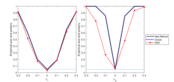
We first compare the performances of and for testing the indirect effect . We set and . The left panel of Figure 1 depicts power functions of the three tests versus the values of over . All the three tests gain larger powers as increases. performs as well as the oracle , and is generally more powerful than . For instance, when , the empirical power of is 0.516, while the empirical powers of and are 0.596. These observations are in consistent with the theoretical results in Section 2.
Next, we turn to test the direct effect. Set . And is taken from , where corresponds to the null hypothesis. The right panel of Figure 1 depicts the power function of the three tests versus the values of over . The proposed test performs almost the same as the oracle one, and is obviously more powerful than the test proposed in Zhou et al. (2020), whose power curve is asymmetric. In fact, when , the empirical powers of our test statistic and the oracle test are about 1, while that of is only about 0.780.
Furthermore, performs unstably according to our simulation studies. To gain insight of this, we explore more on . The estimates and are reported in Table 1 from which it can be seen that the biases of and are very small, while has a large bias. This may be due to that the direct effect is also penalized in Zhou et al. (2020) ’s estimation procedure based on scaled lasso. This makes sense only if the direct effect is expected to be zero. As seen in Table 1, the bias of is very small when , yet inversely when . Table 1 also reports standard errors of corresponding estimates. Both the proposed method and oracle outperform Zhou et al. (2020), especially when estimating .
| New method | Oracle | Zhou et al.’s method | |||||
|---|---|---|---|---|---|---|---|
| -0.8 | 0.5 | ||||||
| -0.4 | 0.5 | ||||||
| 0 | 0.5 | ||||||
| 0.4 | 0.5 | ||||||
| 0.8 | 0.5 | ||||||
| 0.5 | -0.8 | ||||||
| 0.5 | -0.4 | ||||||
| 0.5 | 0 | ||||||
| 0.5 | 0.4 | ||||||
| 0.5 | 0.8 | ||||||
To assess the accuracy of variance estimation of and , Table 2 reports their estimated standard errors in two ways. As to each method - new, oracle and Zhou et al.’s method, the first column lists the empirical standard deviations of point estimates or over 500 replications (they are also recorded in parentheses of Table 1); for the second column, we estimate standard errors of and using formula (2.18) in each simulation run, and reports the average together with standard deviations (in parentheses) over the 500 runs. Note that the R package “freebird” Zhou et al. (2020) does not provide the estimated standard error of . From Table 2, for the new method and oracle, the standard errors estimated by Monte Carlo simulations are close to those calculated from formulas; while the two versions of Zhou et al. (2020) depart more.
| Direct effect () | Indirect Effect () | ||||||||||
| New method | Oracle | New method | Oracle | Zhou et al.’s method | |||||||
| std | se(std) | std | se(std) | std | se(std) | std | se(std) | std | se(std) | ||
| -0.8 | 0.5 | 4.15 | 4.11 | 13.73 | 13.70 | 14.05 | |||||
| -0.4 | 0.5 | 3.13 | 3.08 | 11.98 | 11.95 | 12.20 | |||||
| 0 | 0.5 | 2.99 | 2.99 | 12.61 | 12.63 | 15.00 | |||||
| 0.4 | 0.5 | 3.15 | 3.11 | 11.83 | 11.81 | 12.66 | |||||
| 0.8 | 0.5 | 3.79 | 3.72 | 12.69 | 12.63 | 15.05 | |||||
| 0.5 | -0.8 | 3.38 | 3.37 | 11.62 | 11.64 | 13.13 | |||||
| 0.5 | -0.4 | 3.43 | 3.36 | 12.58 | 12.57 | 13.64 | |||||
| 0.5 | 0 | 3.35 | 3.33 | 12.52 | 12.52 | 13.82 | |||||
| 0.5 | 0.4 | 3.39 | 3.37 | 12.26 | 12.26 | 13.10 | |||||
| 0.5 | 0.8 | 3.29 | 3.26 | 12.10 | 12.17 | 12.86 | |||||
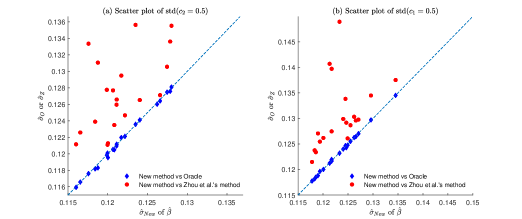
Furthermore, Figure 2 visually compares the standard deviations of over 500 point estimates using the new method (-axis) with those using oracle or Zhou et al.’s method (-axis), respectively. Each blue diamond or red dot in the figure corresponds to each of the 21 different simulation settings - when holding , vary in (a) and holding , vary in (b). The figures imply that the estimated standard errors of the new method are close to oracle, and are generally smaller than those of Zhou et al.’s method. This in turn intuitively illustrates the precision of proposed estimators.
Lastly, Table 3 reports the computing times, where the new method is nearly 1000 times faster than Zhou et al.’s method. The proposed method is very fast and stable because initialized by LASSO estimator, LLA algorithm converges in one step.
| New method | Zhou et al.’s method | ||
|---|---|---|---|
| -0.8 | 0.5 | 1.38 | 1,207.88 |
| -0.4 | 0.5 | 1.47 | 1,327.82 |
| 0 | 0.5 | 1.31 | 1,197.66 |
| 0.4 | 0.5 | 1.52 | 1,614.84 |
| 0.8 | 0.5 | 1.22 | 1,332.24 |
| 0.5 | -0.8 | 1.35 | 1,192.32 |
| 0.5 | -0.4 | 1.33 | 1,329.48 |
| 0.5 | 0 | 1.48 | 1,544.23 |
| 0.5 | 0.4 | 1.50 | 1,790.34 |
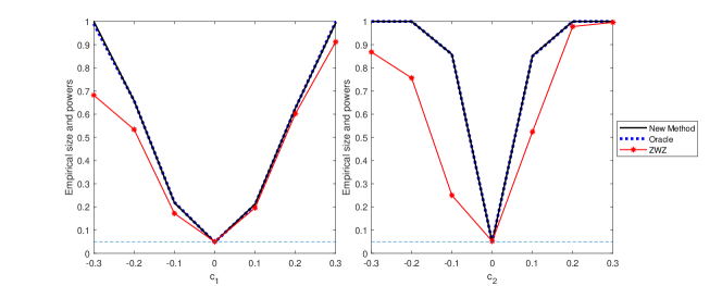
Example 2. In this example, we examine the finite sample performances of proposed method when heavy-tail errors are encountered. Specifically, assume now . The multiplier ensures the equality of variance of to that when . All other settings are identical to those in Example 1. We first investigate the performances of and for testing indirect effect via the left panel of Figure 3. The proposed test performs as well as the oracle one in terms of controlling Type-I error rate () and possessing much larger power than (when ), especially when . Similar phenomenons are observed in the right penal of Figure 3 when examining and . The proposed test performs as well as the oracle one, and is more powerful than the test . In fact, when , the empirical powers of our test statistic and the oracle test are about 1, while that of is only about 0.756. In addition, we also evaluate the accuracy and precision of and through Tables 4 and 5. The overall pattern in these two tables with is very similar to that for . In sum, the proposed method retains its validity for heavy-tailed error distributions.
| New method | Oracle | Zhou et al.’s method | |||||
|---|---|---|---|---|---|---|---|
| -0.8 | 0.5 | ||||||
| -0.4 | 0.5 | ||||||
| 0 | 0.5 | ||||||
| 0.4 | 0.5 | ||||||
| 0.8 | 0.5 | ||||||
| 0.5 | -0.8 | ||||||
| 0.5 | -0.4 | ||||||
| 0.5 | 0 | ||||||
| 0.5 | 0.4 | ||||||
| 0.5 | 0.8 | ||||||
| Direct effect () | Indirect Effect () | ||||||||||
| New method | Oracle | New method | Oracle | Zhou et al.’s method | |||||||
| std | se(std) | std | se(std) | std | se(std) | std | se(std) | std | se(std) | ||
| -0.8 | 0.5 | 4.06 | 3.93 | 12.46 | 12.43 | 12.84 | |||||
| -0.4 | 0.5 | 1.93 | 1.89 | 6.24 | 6.23 | 6.43 | |||||
| 0 | 0.5 | 3.03 | 3.01 | 12.21 | 12.21 | 12.74 | |||||
| 0.4 | 0.5 | 3.29 | 3.26 | 12.30 | 12.29 | 13.01 | |||||
| 0.8 | 0.5 | 3.07 | 3.02 | 6.67 | 6.63 | 7.15 | |||||
| 0.5 | -0.8 | 3.44 | 3.40 | 12.34 | 12.33 | 12.89 | |||||
| 0.5 | -0.4 | 3.45 | 3.41 | 12.32 | 12.30 | 16.26 | |||||
| 0.5 | 0 | 3.42 | 3.41 | 12.34 | 12.30 | 12.95 | |||||
| 0.5 | 0.4 | 3.44 | 3.41 | 12.39 | 12.33 | 12.98 | |||||
| 0.5 | 0.8 | 3.44 | 3.41 | 12.32 | 12.30 | 13.07 | |||||
3.2 Real data analysis
We apply the proposed method to an empirical analysis to examine whether financial statements items and metrics mediate the relationship between company sectors and stock price recovery after COVID-19 pandemic outbreak. While investors and researchers have reached a consensus ages ago that stock returns highly rely on companies’ belonging sectors, recent studies more focus on using financial statements or market conditions to predict stock returns. Fama & French (1993)’s pioneering proposal of the three-factor model started this era, which captures patterns of return using market return, firm size and book-to-market ratio factors. Callen & Segal (2004) showed that accruals, cash flow, growth in operating income significantly influence stocks return. Edirisinghe & Zhang (2007, 2008) developed a relative financial strength metric based on data envelopment analysis (Farrell, 1957; Charnes et al., 1978), and found that return on assets and solvency ratio has high correlation with stock price return. To enhance prediction accuracy, deep neural network and data mining techniques were developed, with model inputs as historical financial statements and output as stock price return (Enke & Thawornwong, 2005; Huang et al., 2019; Lee et al., 2019). Meanwhile, it is reasonable to hypothesize that companies’ sectors affect stock performances via influencing the associated financial metrics. Few existing works, however, study the mediating effects of such financial metrics. Hence our analysis aims to fill in this gap, and use the proposed mediation analysis to select important financial metrics, as well as to test the direct and indirect effects of companies’ sectors on returns.
In addition, we in this analysis are specifically interested in the stock performance of S&P 500 component companies during the COVID-19 pandemic period. As is known, the outbreak of the COVID-19 dealt a shock to the U.S. economy with unprecedented speed, and the government had to take a lockdown to stop spread of virus. The lockdown took a toll in the U.S. economy: business were closed, millions of people lost jobs and the price of an oil futures contract fell below zero. The crisis spread to the U.S. stock market, dragging down the major index S&P 500 by 33.92%. To help businesses, households and the economy, the Federal Reserve and the White House launched various rescue programs and take measures to stabilize energy prices from the end of March, 2020. Therefore, all these events and measures led the U.S. stock market to a V-shape pattern, thanks to which, the general financial rules from classical literature may not directly apply any more.
Admittedly, a number of recent literature studied the economic reaction to COVID-19 pandemic from sector or company level data (Ramelli & Wagner, 2020; Zhang et al., 2020; Baker et al., 2020; Gormsen & Koijen, 2020; De Vito & Gómez, 2020). Thorbecke (2020) analyzed sector-specific and macroeconomic variables as contributing factors to stock return in COVID-19 downturn and found that idiosyncratic factors negatively affected energy and consumer cyclical sectors. Hassan et al. (2020) investigated companies’ transcripts of quarterly earnings call from January to September 2020 to investigate senior management’s and major market participants’ opinions about future prospects. They discovered several important factors related to accounting and business fundamentals, including supply chain, production and operations and financing, that are highly associated with stock market recovery from COVID-19. However, these methods mainly rely on prior financial knowledge to select low dimensional data for modeling, while ignore important company level factors. Besides, these methods only consider the relation of stock return to either sector level or company level while failing to recognize that the company’s financial plays a role in mediating stock sector effects to stock price return. Therefore, we use the proposed method to study the financial statement items or metrics that mediate the relationship between firm sectors and stock performance in this special period. This work may then shed light on how to select valuable stocks during a pandemic or any adverse event likewise.
In the mediation models, the response is taken to be the stock return from its highest price before the pandemic in February, 2020 to April 30th, 2020. The closed price is adjusted for both dividends and splits. The potential mediators in are 550 accounting metrics from financial statements of associated companies, scratched from Yahoo Finance on April 30, 2020. We obtain firms’ annual reports from fiscal year 2015 to 2019 and the first three quarterly reports in 2019. We use the firms’ latest annual report to compute financial metrics and use previous annual reports to compute average growth rate of each financial metrics. The exposure variables in , are companies’ sectors according to Global Industry Classification Standard (GICS) that are coded as dummy variables. GICS classifies companies into eleven sectors: basic materials, communication services, consumer cyclical, consumer defensive, energy, financial services, healthcare, industrials, real estate, technology and utilities. We set energy sector as baseline level.
Table 6 presents the estimated direct and indirect effects of companies’ sectors, together with their standard errors. We also calculate Wald’s test for the indirect effect and generalized likelihood test for direct effect, with -values smaller than and , respectively, indicating both the direct and indirect effect are significant. As for direct effect, stocks in sectors such as healthcare and technology are more likely to outperform benchmark than ones from utilities sector. Furthermore, sectors influence the stocks performance partly through business operation reflected by selected financial metrics, and the indirect effects are significantly positive.
| Sectors | Direct effect | std | Indirect effect | std |
|---|---|---|---|---|
| Intercept | -0.4634 | 0.1558 | -0.5216 | 0.1016 |
| Basic materials | 0.5725 | 0.2226 | 0.4450 | 0.1407 |
| Communication services | 0.9231 | 0.2698 | 0.4227 | 0.1691 |
| Consumer cyclical | 0.0793 | 0.1805 | 0.4154 | 0.1165 |
| Consumer defensive | 0.9808 | 0.2087 | 0.6265 | 0.1386 |
| Financial services | 0.1363 | 0.1844 | 0.3452 | 0.1206 |
| Healthcare | 1.0176 | 0.1887 | 0.7601 | 0.1232 |
| Industrials | 0.3658 | 0.1816 | 0.5899 | 0.1181 |
| Real.Estate | 0.0736 | 0.2185 | 0.5010 | 0.1365 |
| Technology | 0.6537 | 0.1823 | 0.7655 | 0.1203 |
| Utilities | 0.6798 | 0.2121 | 0.3717 | 0.1343 |
| -value |
The selected mediating metrics, their associated estimated coefficients in model (2.1), as well as their brief descriptions, are presented in Table 7. These selected metrics are of their own significance. For instance, the first three chosen metrics in Table 7, namely return on assets, gross margin and annual growth rate of operating income, reflect firms’ revenue. Return on assets is an indicator of how well a firm utilizes its assets, by determining how profitable a firm is relative to its total assets. A firm with a higher return-on-assets value is preferred, as the firm squeezes more out of limited resources to make a profit. Gross margin is the portion of sales revenue a firm retains after subtracting costs of producing the goods it sells and the services it provides. It measures the gross profit of a firm. A firm that has higher gross margin is more likely to retain more profit for every dollar of good sold. Annual growth rate of operating income shows the firm’s growth of generating operating income compared with previous year. Operating income measures the amount of profit realized from a business’s operation, after deducting operating expenses such as wages, depreciation, and cost of goods sold. A firm with high growth of operating income can avoids unnecessary production costs, and improve core business efficiency. In a word, a firm with higher return on assets, gross margin and growing operating income is considered profitable, and hence, is likely to attract investors.
On the other hand, both the average growth rate of quick ratio and debt to assets are indicators of financial leverage of a firm. Quick ratio of a firm is defined as the dollar amount of liquid assets dividing that of current liabilities, where liquid assets are the portion of assets that can be quickly converted into cash with minimal impact on the price received in open market, while current liabilities are a firm’s debts or obligations to be paid to creditors within one year. Thus a large quick ratio indicates that the firm is fully equipped with enough assets to be instantly liquidated to pay off its current liabilities. Debt to assets is the total amount of debt relative to assets owned by a firm. It reflects a firm’s financial stability. Therefore, a firm with a higher quick ratio or a lower debt to assets might be more likely to survive when it is difficult to finance through borrowing and cover its debts, thus are more favorable to investors during the economy lockdown.
Lastly, receivables turnover quantifies a firm’s effectiveness in collecting its receivables or money owed by clients. It shows how well a firm uses and manages the credit it extends to customers and how quickly that short-term debt is paid. Receivables turnover can be negative when net credit sale is negative because the client pre-pay for the product or service. A negative receivables turnover means that the firm are less susceptible to counter-party credit risk because it already receives the cash from its client before delivering the service or shipping out the product. This is especially important during liquidity dry periods when the clients may default or delay payment due to lack of cash. Therefore, a firm that has a negative receivables turnover is preferred.
On all accounts, one might incorporate the analysis results as reference when seeking for a stock portfolio during the financial crisis caused by pandemic. First, the sectors in ‘Healthcare’, ‘Consumer defensive’, ‘Communication service’, ‘Utility’ and ‘Technology’ have the top five positive direct effects on stock return. In terms of the financial metrics, we may focus on those reported in Table 7 to filter stocks. For example, we shall select firms that have higher values in AGR operating income, gross margin, quick ratio, and return on assets but lower values in debt to assets and receivable turnover.
| Selected mediator | Estimated coefficient (std) | Description |
|---|---|---|
| Return on assets | 0.4246 (0.0379) | Net income divided by the total assets |
| Gross margin | 0.0841 (0.0393) | The difference between the revenue and cost of goods sold divided by revenue |
| AGR* Operating Income | 0.1063 (0.0347) | Revenues subtract the cost of goods sold and operating expenses |
| AGR* Quick ratio | 0.1194 (0.0345) | Total current assets minus inventory divided by total current liabilities |
| Debt to assets | -0.1209 (0.0369) | Total debts divided by total assets |
| Receivables turnover (days) | -0.0947 (0.0346) | Average receivables divided by net credit sales times 360 days |
* AGR: average growth rate, calculated as the average of growth rates for the metrics from 2015 to 2019.
Moreover, we compare our findings with those selected in established models. For instance, our method picks profitability factors like return on assets, which is also selected in Fama & French (2015), as profitability is the core of a firm’s stock performance. But we do not include metrics representing size of firm, valuation of stock price or investment that were covered by Fama & French (2015). For firm size factor, there is no evidence that small-size firms recovered faster or slower than larger-size ones. For valuation of stock price factor, previous price valuation ratio changed significantly due to stock price change and is no longer reliable to predict future stock return. For investment factor, it is less important for a short-term stock price movement. Compared with Edirisinghe & Zhang (2008), our method also picks profitability (return on assets), liquidity (quick ratio) and solvency (debt to assets) metrics, as in Edirisinghe & Zhang (2008). During the crisis, a firm facing liquidity crunch could not access to credit. Therefore, a firm with sufficient cash and less debt is more easily to survive and less likely to be forced to liquidate valuable assets at unfavorable prices. And its stock would be safer and more attractive to investors. But we did not select metrics of earnings per share or about capital intensity as in Edirisinghe & Zhang (2008). The lockdown dramatically changes a firm’s revenue structure and capital allocation, and hence reduces predictive capability of these metrics to short-term recovery.
4 Conclusion
In this paper, we propose statistical inference procedures for the indirect effects in high dimensional mediation model. We introduce a partial penalized least squares method and study its statistical properties under random design. We show that the proposed estimators are more efficient than existing ones. We further propose a partial penalized Wald test to detect the indirect effect, with a limiting null distribution. In this paper, we also propose an -type test for the direct effect and reveal Wilks phenomenon in the high-dimensional mediation model. We further utilize the proposed inference procedures to analyze the mediation effects of various financial metrics on the relationship between company’s sector and the stock return.
Acknowledgement
Guo and Liu’s research was supported by grants from National Natural Science Foundation of China grants 12071038, 11701034, and 11771361, and Li and Zeng’s research was supported by National Science Foundation, DMS 1820702, 1953196 and 2015539.
Appendix
A.1 Proofs of Theorems
Define
Proof of Theorem 1: To enhance the readability, we divide the proof of Theorem 1 into three steps. In the first step, we show that there exists a local minimizer of with the constraints , such that . In the second step, we prove that is indeed a local minimizer of . This implies . In the final step, we derive the asymptotic expansion of .
Step 1: Consistency in the -dimensional subspace: We first constrain on the -dimensional subspace of . This constrained partial penalized least squares function is given by
Here and . We now show that there exists a strict local minimizer of such that . To this end, we consider an event
where with , and denotes the boundary of the closed set . Clearly, on the event , there exists a local minimizer of in . Thus, we only need to show that as when is large. To this aim, we next analyze the function on the boundary .
For any , it follows from a second order Taylor’s expansion that
| (A.1) |
Here
and
where lies in the line segment jointing and , and is a diagonal matrix with nonnegative diagonal elements. Clearly . By condition (A2), the maximum eigenvalue of is upper bounded by . Recall that
Further note that
Thus , when .
Since and , we have:
| (A.5) |
Consequently, we obtain
By the Markov inequality, it entails that
| (A.6) |
In the following, we aim to show that .
Note that
Then by condition (A1),
It follows from the concavity of , , and condition (A2) that:
Consequently, step 1 is completed.
Step 2: Sparsity: According to Theorem 1 in Fan and Lv (2011), it suffices to show that with probability tending to 1, we have:
| (A.9) |
Here satisfies that and . Note that
| (A.10) |
For the second term,
Next we come to determine the rate of the first term .
Let with being large enough and note that
We have
Firstly consider the term . Note that are independent centered random variables a.s. bounded by in absolute value. Then the Bernstein inequality yields that
Next we turn to consider . First note that
Further note that
We then conclude that
From this, we then have
Thus .
Consequently, given condition A2, step 2 is finished.
Step 3: Asymptotic expansions: Steps 1 and 2 show that with probability tending to 1, and further .
First denote
| (A.15) |
For , denote
| (A.20) |
Notice that
Or equivalently we have
Recall that , and . Then we have
when . Thus, we have
Under condition (A2), we have . This implies that
By the concavity of and condition (A2), we obtain that
Since , it follows that
| (A.21) |
Proof of Corollary 1: Recall that
Here .
As a result, it follows that
| (A.23) | |||||
The asymptotic variance matrix of is
Recall that
| (A.24) |
Consequently we obtain that
| (A.25) | |||||
Here and .
It is easy to show that Similarly, we have
Further we obtain that , , and
As a result, it follows that
| (A.26) |
Proof of Theorem 2: Similar to the arguments in the proof of Theorem 1, we can also show that with probability 1, and further .
Denote and
It is noted that
| (A.32) |
Here .
From the proof of Theorem 1, it is known that and similarly . Further recall that and . Thus under condition that , we have
| (A.39) |
from which we have
| (A.40) |
Note that from Corollary 1. Thus we get , which further implies that .
Now we are ready to investigate the asymptotic distribution of . Under the event and recalling equation (A.40), we can show that
| (A.41) | |||||
Now denote . It is easy to know that . From the proof of Corollary 1, it is known that Thus we obtain that
| (A.42) |
On the other hand, we have
It is easy to know that , while . Further note that
In sum, it follows that
| (A.43) |
As a result, we have
A.2 Natural direct and indirect effects
Under the independence conditions of random errors in the models, the sequential ignorability assumption (Imai et al., 2010) holds, and the natural direct and indirect effects can be identified. As argued by Imai et al. (2010), only the sequential ignorability assumption is needed and neither the linearity nor the no-interaction assumption is required for the identification of mediation effects. However, in the situation with high dimensional mediators, it would be very challenging if not impossible to make inference about the mediation models without linearity nor the no-interaction assumption. The linearity and the no-interaction assumptions are widely adopted in recent studies about HDMM (Zhang et al., 2016; van Kesteren & Oberski, 2019; Zhou et al., 2020).
To define the natural direct and natural indirect effects, we give some notation first. Let denote the potential outcome that would have been observed had and been set to and , respectively, and denotes the potential mediator that would have been observed had been set to . Following Imai et al. (2010); Vanderweele & Vansteelandt (2014), and others, for versus , the natural direct effect is defined as While the indirect effect is defined as Then the total effect is the sum of the natural direct and indirect effect. Vanderweele & Vansteelandt (2014) showed that
Thus can be interpreted as the average natural direct effect, and can be interpreted as the average natural indirect effect, of a one-unit change in the exposure .
References
- Abarbanell & Bushee (1997) Abarbanell, J. S., & Bushee, B. J.(1997). Fundamental analysis, future earnings, and stock prices. Journal of Accounting Research, 35(1), 1-24.
- Ai et al. (2021) Ai, C., Linton, O. & Zhang, Z.(2021). Estimation and inference for the counterfactual distribution and quantile functions in continuous treatment models. Journal of Econometrics, https://doi.org/10.1016/j.jeconom.2020.12.009.
- Athey et al. (2018) Athey, S., Imbens, G. & Wager, S.(2018). Approximate residual balancing: Debiased inference of average treatment effects in high dimensions. Journal of the Royal Statistical Society, Series B 80, 597-623.
- Baron & Kenny (1986) Baron, R. M. & Kenny, D. A.(1986). The moderator-mediator variable distinction in social psychological research: Conceptual, strategic, and statistical considerations. Journal of Personality and Social Psychology 51(6), 1173-1182.
- Baker et al. (2020) Baker, S. R., Bloom, N., Davis, S. J., Kost, K., Sammon, M., & Viratyosin, T.(2020). The unprecedented stock market reaction to COVID-19. The Review of Asset Pricing Studies, 10(4), 742-758.
- Belloni et al. (2014) Belloni, A., Chernozhukov, V. & Hansen, C.(2014). Inference on treatment effects after selection among high-dimensional controls. The Review of Economic Studies 81(2), 608-650.
- Callen & Segal (2004) Callen, J. L., & Segal, D. (2004). Do accruals drive firm‐level stock returns? A variance decomposition analysis. Journal of Accounting Research, 42(3), 527-560.
- Chakrabortty et al. (2018) Chakrabortty, A., Nandy, P. & Li, H.(2018). Inference for individual mediation effects and interventional effects in sparse high-dimensional causal graphical models. arXiv: 1809.10652v1.
- Charnes et al. (1978) Charnes, A., Cooper, W. W., & Rhodes, E.(1978). Measuring the efficiency of decision making units. European Journal of Operational Research, 2(6), 429-444.
- Chen et al. (2018) Chen, O. Y., Crainiceanu, C., Ogburn, E. L., Caffo, B. S., Wager, T. D. & Lindquist, M. A. (2018). High-dimensional multivariate mediation with application to neuroimaging data. Biostatistics 19(2), 121-136.
- Chernozhukov et al. (2021) Chernozhukov, V., Kasahara, H. J. & Schrimpf, P.(2021). Causal impact of masks, policies, behavior on early covid-19 pandemic in the US. Journal of Econometrics 220(1), 23-62.
- Conti et al. (2016) Conti, G., Heckman, J. J. & Pinto, R. (2016). The effects of two influential early childhood interventions on health and healthy behaviour. The Economic Journal 126(596), 28-65.
- De Vito & Gómez (2020) De Vito, A., & Gómez, J. P.(2020). Estimating the COVID-19 cash crunch: Global evidence and policy. Journal of Accounting and Public Policy, 39(2), 106741.
- Derkach et al. (2019) Derkach, A., Pfeiffer, R. M., Chen, T. H. & Sampson, J. N.(2019). High dimensional mediation analysis with latent variables. Biometrics 75(3), 745-756.
- Dimitropoulos & Asteriou (2009) Dimitropoulos, P. E., & Asteriou, D.(2009). The value relevance of financial statements and their impact on stock prices. Managerial Auditing Journal, 24(3), 248-–265.
- Donald & Hsu (2014) Donald, S. G. & Hsu, Y. C.(2014). Estimation and inference for distribution functions and quantile functions in treatment effect models. Journal of Econometrics 178, 383-397.
- Edirisinghe & Zhang (2007) Edirisinghe, N. C., & Zhang, X.(2007). Generalized DEA model of fundamental analysis and its application to portfolio optimization. Journal of banking & finance, 31(11), 3311-3335.
- Edirisinghe & Zhang (2008) Edirisinghe, N. C. P., & Zhang, X. (2008). Portfolio selection under DEA-based relative financial strength indicators: case of US industries. Journal of the Operational Research Society, 59(6), 842-856.
- Enke & Thawornwong (2005) Enke, D., & Thawornwong, S.(2005). The use of data mining and neural networks for forecasting stock market returns. Expert Systems with Applications, 29(4), 927-940.
- Fama & French (1993) Fama, E. F., & French, K. R. (1993). Common risk factors in the returns on stocks and bonds. Journal of Financial Economics, 33, 3–-56.
- Fama & French (2015) Fama, E. F., & French, K. R.(2015). A five-factor asset pricing model. Journal of Financial Economics, 116(1), 1-22.
- Fan et al. (2012) Fan, J., Guo, S. & Hao, N.(2012). Variance estimation using refitted cross-validation in ultrahigh dimensional regression. Journal of the Royal Statistical Society, Series B 74, 37-65.
- Fan & Li (2001) Fan, J. & Li, R.(2001). Variable selection via nonconcave penalized likelihood and its oracle properties. Journal of the American Statistical Association 96, 1348-1360.
- Fan et al. (2020) Fan, J., Li, R., Zhang, C.-H. & Zou, H.(2020). Statistical Foundations of Data Science. Chapman and Hall/CRC. Boca Raton, FL.
- Fan & Lv (2011) Fan, J. & Lv, J. (2011). Nonconcave penalized likelihood with NP-dimensionality. IEEE Transactions on Information Theory 57, 5467-5484.
- Fan, et al (2020a) Fan, Y., Lv, J., Sharifvaghefi, M. and Uematsu, Y. (2020a). IPAD: stable interpretable forecasting with knockoffs inference. Journal of the American Statistical Association 115, 1822-1834.
- Fan, et al (2020b) Fan, Y., Demirkaya, E., Li, G. and Lv, J. (2020b). RANK: large-scale inference with graphical nonlinear knockoffs. Journal of the American Statistical Association 115, 362-379.
- Farrell (1957) Farrell, M. J.(1957). The measurement of efficiency productive. Journal of the Royal Statistical Society, 120(3), 253-266.
- Gormsen & Koijen (2020) Gormsen, N. J., & Koijen, R. S.(2020). Coronavirus: Impact on stock prices and growth expectations. The Review of Asset Pricing Studies, 10(4), 574-597.
- Graham et al. (2002) Graham, Carol M., Mark V. Cannice, & Todd L. Sayre.(2002) The value‐relevance of financial and non‐financial information for Internet companies. Thunderbird International Business Review, 44(1), 47-70.
- Hassan et al. (2020) Hassan, T. A., Hollander, S., van Lent, L., Schwedeler, M., & Tahoun, A.(2020). Firm-level Exposure to Epidemic Diseases: Covid-19, SARS, and H1N1. National Bureau of Economic Research, No.26971.
- Hayes (2013) Hayes, A. F. (2013). Introduction to Mediation, Moderation, and Conditional Process Analysis: A Regression-based Approach. Guilford Press.
- Huang et al. (2019) Huang, Y., Capretz, L. F., & Ho, D. (2019). Neural network models for stock selection based on fundamental analysis. In 2019 IEEE Canadian Conference of Electrical and Computer Engineering (CCECE) (pp. 1-4). IEEE.
- Huang & Pan (2016) Huang, Y. T. & Pan, W. C.(2016). Hypothesis test of mediation effect in causal mediation model with high-dimensional continuous mediators. Biometrics 72(2), 402-413.
- Huber et al. (2020) Huber, M., Hsu, Y. C., Lee, Y. Y. & Lettry, L.(2020). Direct and indirect effects of continuous treatments based on generalized propensity score weighting. Journal of Applied Econometrics 35(7), 814-840.
- Imai et al. (2010) Imai, K., Keele, L.& Tingley, D.(2010). A general approach to causal mediation analysis. Psychological Methods 15(4), 309-334.
- Imbens (2004) Imbens, G. (2004). Nonparametric estimation of average treatment effects under exogeneity: A review. The Review of Economics and Statistics 86(1), 4-29.
- Javanmard & Montanari (2014) Javanmard, A. & Montanari, A.(2014). Confidence intervals and hypothesis testing for high-dimensional regression. Journal of Machine Learning Research 15(1), 2869-2909.
- Khan & Khokhar (2015) Khan, M. N., & Khokhar, I. (2015). Quarterly Journal of Econometrics Research. Quarterly Journal of Econometrics Research, 1(1), 1-12.
- Lee et al. (2019) Lee, T. K., Cho, J. H., Kwon, D. S., & Sohn, S. Y.(2019). Global stock market investment strategies based on financial network indicators using machine learning techniques. Expert Systems with Applications, 117, 228-242.
- Mackinnon (2008) Mackinnon, D. P. (2008). Introduction to Statistical Mediation Analysis. Routledge
- Preacher (2015) Preacher, K. J. (2015). Advances in mediation analysis: A survey and synthesis of new developments. Annual Review of Psychology 66(1), 825-852.
- Preacher & Hayes (2008) Preacher, K. J. & Hayes, A. F. (2008). Asymptotic and resampling strategies for assessing and comparing indirect effects in multiple mediator models. Behavior Research Methods 40(3), 879-891.
- Ramelli & Wagner (2020) Ramelli, S., & Wagner, A. F. (2020). Feverish stock price reactions to COVID-19. The Review of Corporate Finance Studies, 9(3), 622-655.
- Shi et al. (2019) Shi, C., Song, R., Chen, Z., & Li, R. (2019). Linear hypothesis testing for high-dimensional generalized linear model. Annals of Statistics 47(5), 2671-2703.
- Song et al. (2020) Song, Y., Zhou, X., Zhang, M., Zhao, W., Liu, Y., Kardia, S. L. R., Roux, A. V. D., Needham, B. L., Smith, J. A. & Mukherjee, B.(2020). Bayesian shrinkage estimation of high dimensional causal mediation effects in omics studies. Biometrics 76(3), 700-710.
- Sun & Zhang (2013) Sun, T. & Zhang, C. H. (2013). Scaled sparse linear regression. Biometrika 99(4), 879-898.
- Ten Have & Joffe (2010) Ten Have, T. & Joffe, M. (2010). A review of causal estimation of effects in mediation analyses. Statistical Methods in Medical Research 21(1), 77-107.
- Thorbecke (2020) Thorbecke, W.(2020) The Impact of the COVID-19 Pandemic on the US Economy: Evidence from the Stock Market. Journal of Risk and Financial Management, 13(10), 233.
- van de Geer et al. (2014) van de Geer, S., Buhlmann, P., Ritov, Y. & Dezeure, R. (2014). On asymptotically optimal confidence regions and tests for high-dimensional models. Annals of Statistics 42(3), 1166-1202.
- van Kesteren & Oberski (2019) van Kesteren, E. J. & Oberski, D. L.(2019). Exploratory mediation analysis with many potential mediators. Structural Equation Modeling: A Multidisciplinary Journal 26(5), 710-723.
- Vanderweele (2015) Vanderweele, T. J.(2015). Explanation in Causal Inference: Methods for Mediation and Interaction. Oxford University Press. New York.
- Vanderweele & Vansteelandt (2014) Vanderweele, T. J. & Vansteelandt, S.(2014). Mediation analysis with multiple mediators. Epidemiologic Methods 2(1), 95-115.
- Wang et al. (2013) Wang, L., Kim, Y. & Li, R.(2013). Calibrating non-convex penalized regression in ultra-high dimension. Annals of Statistics 41(5), 2505-2536.
- Wang et al. (2012) Wang, L., Wu, Y. & Li, R. (2012). Quantile regression for analyzing heterogeneity in ultra-high dimension. Journal of the American Statistical Association 107(497), 214-222.
- Zhang et al. (2020) Zhang, D., Hu, M., & Ji, Q.(2020). Financial markets under the global pandemic of COVID-19. Finance Research Letters, 36, 101528.
- Zhang et al. (2016) Zhang, H., Zheng, Y., Zhang, Z., Gao, T., Joyce, B., Yoon, G., Zhang, W., Schwartz, J., Just, A., Colicino, E., Vokonas, P., Zhao, L., Lv, J., Baccarelli, A., Hou, L. & Liu, L.(2016). Estimating and testing high-dimensional mediation effects in epigenetic studies. Bioinformatics 32(20), 3150-3154.
- Zhang & Zhang (2014) Zhang, C. H. & Zhang, S. S.(2014). Confidence intervals for low dimensional parameters in high dimensional linear models. Journal of the Royal Statistical Society, Series B 76, 217-242.
- Zhao et al. (2020) Zhao, Y. Linqduist, M. A., & Caffo, B.S. (2020). Sparse principal component based high-dimensional mediation analysis. Computational Statistics and Data Analysis 142, 106835.
- Zhou et al. (2020) Zhou, R. X., Wang, L. W., & Zhao, S. H.(2020). Estimation and inference for the indirect effect in high-dimensional linear mediation models. Biometrika 107(3), 573-589.
- Zou & Li (2008) Zou, H. and Li, R. (2008). One-step sparse estimates in nonconcave penalized likelihood models. Annals of Statistics 36(4), 1509-1533.