Multiple Hypothesis Testing Framework for Spatial Signals

Abstract

The problem of identifying regions of spatially interesting, different or adversarial behavior is inherent to many practical applications involving distributed multisensor systems. In this work, we develop a general framework stemming from multiple hypothesis testing to identify such regions. A discrete spatial grid is assumed for the monitored environment. The spatial grid points associated with different hypotheses are identified while controlling the false discovery rate at a pre-specified level. Measurements are acquired using a large-scale sensor network. We propose a novel, data-driven method to estimate local false discovery rates based on the spectral method of moments. Our method is agnostic to specific spatial propagation models of the underlying physical phenomenon. It relies on a broadly applicable density model for local summary statistics. In between sensors, locations are assigned to regions associated with different hypotheses based on interpolated local false discovery rates. The benefits of our method are illustrated by applications to spatially propagating radio waves.

I Introduction

The rapid development of ever cheaper and smaller sensors, as well as the rise of faster, lower latency and more reliable wireless connectivity standards have facilitated the deployment of large-scale wireless sensor networks (WSNs). WSNs are a key technology in the Internet of Things (IoT) and 5G wireless systems to gather information on spatial phenomena. The terms spatial phenomenon or spatial signal refer to the general concept of a physical quantity of interest that is a smooth function of location [1]. These occur in a large number of applications, for example in electromagnetic spectrum awareness, wireless communications, environmental monitoring, agriculture, smart buildings and acoustics. A WSN may be composed of heterogeneous devices with different sensing capabilities. The individual nodes are commonly battery powered and operate in a congested wireless spectrum. Thus, WSNs must communicate their local information from each sensor efficiently in terms of spectrum use and energy consumption [2, 3].

In this work, we develop a method for identifying the spatial regions of interesting, different or anomalous behavior of a spatial signal using WSNs while strictly controlling the error levels. Practical examples for such regions include areas in a city where emission levels are intolerably high, radio frequency bands are densely used/underutilized, regions where moisture is too low in agricultural fields or rooms with unusual oxygen or temperature levels inside a building. Due to the spatial smoothness assumption, these areas form locally continuous subregions. Fig. 1 displays the problem in a simplified manner. We identify these interesting regions by developing methods stemming from detection theory, in particular multiple hypothesis testing (MHT). This allows for providing rigorous statistical performance guarantees independently of domain-specific user knowledge. Minimal assumptions on the underlying physical phenomenon are needed. The sensors are placed sparsely in distinct locations. No particular geometry or configuration is assumed for the distributed sensors. Hence, the proposed method is suitable for a large variety of practical applications.

I-A Limiting the consumption of resources

To the best of our knowledge, none of the existing approaches in the literature on monitoring of spatial fields using WSNs solves the aforementioned problem. However, two areas of research are closely related: field estimation and hypothesis testing for spatial signals. The objective in field estimation is to determine the numerical value of the observed spatial signal (or a transformation of the spatial signal) as a function of location. Field estimation methods usually assume that the sensors transmit all raw local measurements to the fusion center (FC) or the other nodes [1, 4]. This results in significant communication overhead and increased power consumption. To deal with the communication and power constraints for WSNs, many methods for hypothesis testing for spatial signals in WSNs limit the amount of information transmitted from each node to other nodes/the FC. In distributed detection [5], a hard (binary) decision on the local state is communicated to the FC. The local decisions are fused at FC to make a decision on the overall state of the field. Recent works transmit more than a single bit [6, 7, 8, 9, 10, 11, 12]. In line with [2, 13, 14], we allow each sensor to communicate a sufficient statistic or soft decisions quantized using only few bits. This enables the application of advanced MHT methods while requiring (at most) only one communication cycle per sensor.

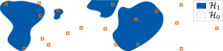
Figure 1: An exemplary spatial inference problem. Squares indicate sensors. The unknown region of interest $\mathcal{H}_{1}$ consists of four spatially continuous subregions (blue).

I-B Enabling localized inference

The existing works on hypothesis testing methods for spatial signals with WSNs focus on the detection of the presence of interesting, different or anomalous behavior of the spatial signal somewhere within entire observation area under guarantees on the error probabilities. The only exception is [15], where the authors also identify the sensors that observe the anomaly. In this work, we consider the more demanding problem of identifying the areas where the spatial signal exhibits different behavior than in nominal conditions such that statistical performance guarantees in terms of Type I error control are provided. To this end, we model the spatial area of interest as a regular spatial grid. We make a decision on the state of the observed phenomenon at each grid point. We discriminate between the nominal state of the phenomenon, represented by the null hypothesis $\mathrm{H}_{0}$, and any state that deviates from the nominal, represented by alternate hypotheses. While in many problems, one could distinguish various classes of anomalous, interesting or different behavior, we summarize everything that is not conform to $\mathrm{H}_{0}$ under the alternative $\mathrm{H}_{1}$.

I-C The necessity of multiple hypothesis testing

Depending on the size of the monitored area and the desired spatial resolution, the number of grid points and hence decisions might easily reach the order of tens of thousands. To prevent a flood of false positives resulting from testing a large number of binary hypotheses [16], we follow the principles of MHT, where choosing the alternative $\mathrm{H}_{1}$ is called a discovery [17]. Performance guarantees are commonly provided using the false discovery rate (FDR) criterion. The FDR is the expected proportion of false discoveries among all discoveries, [18]. The past work on FDR control in the context of spatial data has mostly focused on testing a priori [19, 20] or a posteriori [21, 22, 23, 24] formed groups of data. While these procedures typically rely on assumptions that may not be realistic [25], they do also not provide guarantees w.r.t. to the localization accuracy of the identified alternative area.

I-D Overview on the proposed inference methodology

For decision making with false positive control, information on the state of the field is needed at each grid point. This can be the value of a local decision statistic such as a $p$-value, $z$-score or likelihood ratio in combination with the probability model for this statistic under $\mathrm{H}_{0}$, or the local posterior probability of the null hypothesis. In this work, sensors are placed in distinct locations at a sparse subset of grid points. Each sensor records noisy observations of the field and condenses the information into a local decision statistic. Based on the local decision statistics from each sensor and on the probability model of the local statistic under $\mathrm{H}_{0}$, we compute the probability of the null hypothesis at each grid point where a sensor is located. In particular, we propose to estimate the local false discovery rate (lfdr) [26, 27, 28, 29], which is the empirical Bayes posterior probability of $\mathrm{H}_{0}$ at each sensor. We then exploit the spatial smoothness assumption and interpolate the lfdr’s to make decisions at grid points in between sensors. To the best of our knowledge, this problem has not been addressed in existing works. The main stages of the proposed spatial inference algorithm are shown in Fig. 2. The decisions are made with strict control of the FDR. This provides quantitative justification for the identified areas of different behavior and distinguishes the proposed approach from methods that reconstruct the field and threshold it to get a visually pleasing segmentation result without any statistical error performance guarantees [30].

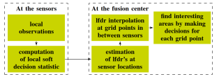
Figure 2: The proposed lfdr-based spatial inference method.

I-E Advantages of the proposed spatial inference approach

The local signal model under $\mathrm{H}_{0}$ may be different in each sensor and it can be learned or its parameters estimated when there is only noise present. This makes the method robust against modeling errors and suitable to a wide range of applications and operational environments. The local signal and noise models may differ, which makes the method suitable for heterogeneous WSNs. The local information is communicated efficiently to the FC. Our results demonstrate that the local soft decision statistics can be quantized using few bits with only a negligible performance loss. Communication overhead and power consumption can be further reduced by censoring the transmission of uninteresting local soft decision statistics. Finally, the detection power of the proposed lfdr-based inference method can be further improved by incorporating available side information similar to [29, 31, 32, 33, 34, 35].

As an alternative approach to obtaining the local null probabilities via lfdr’s, one could imagine a fully integrated method in which the raw measurements or soft decision statistics would feed a model that then provided the local null probabilities at the grid points. However, such a holistic model would depend on a variety of unknown parameters and thus be highly complex. For a radio frequency field, for example, the model would require the appropriate incorporation of the local signal model and position of each sensor, the unknown location and number of active transmitters as well as the propagation environment. In addition, such a model would also be different for each application, thereby limiting its general applicability. To the best of our knowledge, the two existing approaches [36, 37] are not applicable to identify the areas of interesting signal behavior with WSNs while controlling decision making error levels. [36] assumes a simple Gaussian random field model and the authors highlight that the method is very sensitive to model deviations. The method from [37] has been shown in [31] to violate the nominal FDR level. Also, [36, 37] are highly computationally complex even for moderately sized grids.

I-F Challenges

The computation of the lfdr’s relies on the joint probability density function (PDF) of the local soft decision statistics and the overall proportion of alternatives that are unknown in practice. These quantities need to be learned or estimated accurately from the data. This is referred to as lfdr estimation in the MHT literature [29]. A variety of estimators exist, often assuming that the joint PDF belongs to the exponential family [29, 38, 39, 34]. As our simulation results show, the existing lfdr estimators are not suitable for spatial inference with WSNs. They either yield inaccurate lfdr estimates due to too simplistic assumed data models, scale poorly with network size and can thus not be applied to large-scale WSN s and/or yield insufficient results when the local soft decision statistics are quantized with few bits.

I-G The original contributions of this paper

• We propose an lfdr-based spatial inference method for WSNs as a flexible data-driven approach to determine the areas of interest, difference or anomaly of a physical phenomenon. Our proposed method scales well to spatial inference with large-scale sensor networks under strict statistical performance guarantees.

• We propose a novel, highly computationally efficient method for computing lfdr’s. It bases upon an innovative mixture distribution model and the method of moments. It can deal with quantized local soft decision statistics.

I-H Notation

Throughout the paper, regular lowercase letters $x$ denote scalars, whereas bold lowercase letters $\mathbf{x}$, bold uppercase letters $\mathbf{X}$ and underlined bold uppercase letters $\underline{\mathbf{X}}$ denote vectors, matrices and third order tensors, respectively. $\mathbf{X}^{\frac{1}{2}}$ and $\mathbf{X}^{\dagger}$ denote matrix square root and Moore-Penrose inverse. Calligraphic letters $\mathcal{X}$ denote sets and $[X]\coloneqq 1,2,\dots,X$ sets containing all positive integers $\leq X$. $|\mathcal{X}|$ is the cardinality of set $\mathcal{X}$ and $\mathbbm{1}\!\left\{\cdot\right\}$ denotes the indicator function. The Hadamard product operator is $\odot$, while $\circ$ represents the outer product. $f_{X}(x)$ denotes the PDF of random variable (RV) $X$ and $f_{X|\mathrm{A}}(x)$ its PDF conditioned on event $\mathrm{{A}}$.

II The spatial inference problem

The spatial inference problem is illustrated in Fig. 1. $\mathcal{H}_{0}$ and $\mathcal{H}_{1}$ denote the regions of nominal and anomalous, different or interesting behavior, respectively. The continuous observation area is discretized by a regular grid of $Q$ elements, to each of which we refer by its index $q\in[Q]$. Their position on the grid is denoted by $\mathbf{c}_{q}=[c_{\text{x},q},c_{\text{y},q}]^{\top}$. Sensors are placed at $N\leq Q$ grid points. To keep the notation simple, we use the same ordering in the indices of sensors and grid points, i.e., the sensor $n\,\forall\,[N]$ is located at grid point $q=n$. The state of the observed phenomenon at grid point $q\in[Q]$ and time instant $t\in[T]$ is described by the unknown true binary local hypothesis $H_{q,t}\in\{\mathrm{H}_{0},\mathrm{H}_{1}\}$, with the null hypothesis $\mathrm{H}_{0}$ and the alternative $\mathrm{H}_{1}$. If $H_{q,t}=\mathrm{H}_{0}$, we say that the observed phenomenon is in its nominal state at $q\in[Q]$, $t\in[T]$. If $H_{q,t}=\mathrm{H}_{1}$, an interesting phenomenon or anomaly is present. $\mathrm{H}_{1}$ holds under any deviation from $\mathrm{H}_{0}$ and is thus in general composite. In environmental monitoring, $\mathrm{H}_{0}$ could represent clean air, whereas $\mathrm{H}_{1}$ could indicate contamination above a tolerable level. We consider phenomena that vary smoothly in space and slowly in time. Due to the latter, we assume that the true local hypotheses are constant over the observation period and write $H_{q}=H_{q,t}\,\forall\,t\in[T]$.

$\mathcal{H}_{1}$ and $\mathcal{H}_{0}$ are mutually exclusive sets that comprise the grid points at which $\mathrm{H}_{0}$ or $\mathrm{H}_{1}$ hold. Formally, the objective of spatial inference is to identify the set $\mathcal{H}_{0}=\{q\in[Q]\,|\,H_{q}=\mathrm{H}_{0}\}$ of all grid points where $\mathrm{H}_{0}$ is in place, and the set $\mathcal{H}_{1}=\{q\in[Q]\,|\,H_{q}=\mathrm{H}_{1}\}$ containing all locations where $\mathrm{H}_{1}$ holds. At the sensors, the hypothesis-dependent models for the measured field levels $y_{{\color[rgb]{0,0,0}n}}(t),{\color[rgb]{0,0,0}n}\in[{\color[rgb]{0,0,0}N}],t\in[T],$ are

$$\begin{split}{\color[rgb]{0,0,0}H_{n}}=\mathrm{H}_{0}:\qquad\qquad&y_{{\color[rgb]{0,0,0}n}}(t)={\color[rgb]{0,0,0}\delta}_{{\color[rgb]{0,0,0}n}}(t),\\ {\color[rgb]{0,0,0}H_{n}}=\mathrm{H}_{1}:\qquad\qquad&y_{{\color[rgb]{0,0,0}n}}(t)=x_{{\color[rgb]{0,0,0}n}}+{\color[rgb]{0,0,0}\delta}_{{\color[rgb]{0,0,0}n}}(t),\end{split}$$ (1)

where $x_{{\color[rgb]{0,0,0}n}}\neq 0$ is the non-zero level of the phenomenon at location $n$ and ${\color[rgb]{0,0,0}\delta}_{{\color[rgb]{0,0,0}n}}(t)$ the temporally i.i.d. measurement noise. This noise process is spatially independent but not necessarily identically distributed in different nodes. $x_{{\color[rgb]{0,0,0}n}}$ varies with ${\color[rgb]{0,0,0}n}\in[{\color[rgb]{0,0,0}N}]$, but takes on similar values at close-by locations due to the spatial smoothness assumption. This is well-justified by the underlying mechanisms of many physical phenomena. Radio waves, for example, are subject to path-loss and shadow fading [40] that vary slowly. We cannot directly observe $H_{q},\,q\in[Q]$. However, we can exploit the model differences in Eq. (1) to determine local decision statistics for each grid point $q\in[Q]$ based on the measurements at each sensor $n\in[N]$. Those can then be used to decide on $\hat{H}_{q}=\mathrm{H}_{0}$ or $\hat{H}_{q}=\mathrm{H}_{1}$ and form the estimated regions $\hat{\mathcal{H}}_{0}$ and $\hat{\mathcal{H}}_{1}$ associated with null hypothesis and alternative. The decisions are made such that the FDR [18], the expected ratio between the number of false discoveries and all discoveries

$$\operatorname{FDR}=\operatorname{E}\left[\frac{\sum_{q\in\mathcal{H}_{0}}\mathbbm{1}\!\left\{\hat{H}_{q}=\mathrm{H}_{1}\right\}}{\sum_{q=1}^{Q}\mathbbm{1}\!\left\{\hat{H}_{q}=\mathrm{H}_{1}\right\}}\right],$$ (2)

is controlled at a nominal level $\alpha$. This guarantees that on average, a proportion $(1-\alpha)$ of the locations in $\hat{\mathcal{H}}_{1}$ are actual members of the true alternative region $\mathcal{H}_{1}$.

Each sensor condenses its raw measurements over the observation period $T$ into a local summary statistic $\tau_{{\color[rgb]{0,0,0}n}},{\color[rgb]{0,0,0}n}\in[{\color[rgb]{0,0,0}N}]$. The type of deployed sensor and the distribution of the measurement noise may differ from sensor to sensor [41]. Thus, the $\tau_{{\color[rgb]{0,0,0}n}}$ cannot be directly fused with each other. Instead, one defines local (soft) decision statistics $S_{{\color[rgb]{0,0,0}n}}$ that are normalized such that they are i.i.d. $\forall\,{\color[rgb]{0,0,0}n}\in\mathcal{H}_{0}$, but not necessarily for ${\color[rgb]{0,0,0}n}\in\mathcal{H}_{1}$. Conditioned on the field level $x_{{\color[rgb]{0,0,0}n}}$, however, the $S_{n}$ from sensors where $\mathrm{H}_{1}$ is in place are independently distributed. $\mathcal{F}$ denotes the domain of $S_{{\color[rgb]{0,0,0}n}}$. Common choices are $p$-values

$$S_{{\color[rgb]{0,0,0}n}}\coloneqq\int_{{\color[rgb]{0,0,0}\uptau_{n}}}^{\infty}f_{\tau_{{\color[rgb]{0,0,0}n}}|\mathrm{H}_{0}}(\tau)\mathrm{d}\tau=P_{{\color[rgb]{0,0,0}n}},$$ (3)

$\forall\,{\color[rgb]{0,0,0}n}\in[{\color[rgb]{0,0,0}N}]$, where $f_{\tau_{q}|\mathrm{H}_{0}}({\color[rgb]{0,0,0}\tau})$ is the PDF of $\tau_{q}$ under ${\color[rgb]{0,0,0}H_{n}}=\mathrm{H}_{0}$ and $\uptau_{n}$ is a realization of random variable $\tau_{n}$, or $z$-scores $S_{{\color[rgb]{0,0,0}n}}\coloneqq\Phi^{-1}(P_{{\color[rgb]{0,0,0}n}})=Z_{{\color[rgb]{0,0,0}n}}$, where $\Phi(\cdot)$ is the standard normal cumulative distribution function (CDF) [29]. For $p$-values, the domain is $\mathcal{F}=[0,1]$ and for $z$-scores, $\mathcal{F}=\mathbb{R}$. $f_{\tau_{{\color[rgb]{0,0,0}n}}|\mathrm{H}_{0}}(\tau)$ has to be known to compute $p$-values or $z$-scores. If $f_{\tau_{{\color[rgb]{0,0,0}n}}|\mathrm{H}_{0}}(\tau)$ is unknown, it can be estimated from the data using for example the bootstrap [42, 43]. Small $p$-values indicate little support for $\mathrm{H}_{0}$. The soft decision statistics are transmitted from each sensor to the FC via a wireless communication channel and have to be quantized in practice. Similar to [2, 13, 14], the proposed inference method is designed assuming the availability of infinitely precise local soft decision statistics at the FC. However, our results in Sec. VII underline, that close to optimal performance is achieved even when the local soft decision statistics are quantized using only few bits.

Define the random variable $S$ that represents the mixture of all local decision statistics from the sensors. The PDF of $S$ is

$$f_{S}(s)=\pi_{0}f_{S|\mathrm{H}_{0}}\!(s)+{\color[rgb]{0,0,0}\frac{{\color[rgb]{0,0,0}(1-\pi_{0})}}{{\color[rgb]{0,0,0}\sum_{n\in\mathcal{H}_{1}}}1}}\sum_{{\color[rgb]{0,0,0}n}\in\mathcal{H}_{1}}f_{S_{{\color[rgb]{0,0,0}n}}|\mathrm{H}_{1}}(s),$$ (4)

with $\pi_{0}={\color[rgb]{0,0,0}\sum_{n\in\mathcal{H}_{0}}1/N}$ the fraction of sensors located in the null region, $f_{S|\mathrm{H}_{0}}\!(s)$ the PDF for $S_{{\color[rgb]{0,0,0}n}}\,\forall\,{\color[rgb]{0,0,0}n}\in\mathcal{H}_{0}$ and $f_{S_{{\color[rgb]{0,0,0}n}}|\mathrm{H}_{1}}(s)$ the PDF for $S_{{\color[rgb]{0,0,0}n}}$ if ${\color[rgb]{0,0,0}n}\in\mathcal{H}_{1}$. The model in Eq. (4) exploits that the local decision statistics are i.i.d. across locations ${\color[rgb]{0,0,0}n}\in\mathcal{H}_{0}$. Finally, the local false discovery rate is [27, 29]

$$\mathrm{lfdr}(s)=\frac{\pi_{0}f_{S|\mathrm{H}_{0}}\!(s)}{f_{S}(s)}.$$ (5)

Appealingly, $\mathrm{lfdr}_{{\color[rgb]{0,0,0}n}}=\mathrm{lfdr}(s_{{\color[rgb]{0,0,0}n}})$ is the posterior empirical Bayes probability that ${\color[rgb]{0,0,0}n}\in\mathcal{H}_{0}$. We interpolate the $\mathrm{lfdr}_{n}$ to obtain $\mathrm{lfdr}_{q}$ for each grid point $q\in[Q]$ in between sensors. To solve the spatial inference problem while controlling $\operatorname{FDR}\leq\alpha$, we form the region associated with the alternative hypothesis

$$\hat{\mathcal{H}}_{1}=\underset{\mathcal{H}\subseteq[Q]}{\mathrm{argmax}}\bigg{\{}|\mathcal{H}|:{\color[rgb]{0,0,0}\frac{1}{|\mathcal{H}|}}\sum_{q\in\mathcal{H}}\mathrm{lfdr}_{q}\leq\alpha\bigg{\}}.$$ (6)

This approach guarantees FDR control at level $\alpha$ while maximizing detection power, since the so-called Bayesian false discovery rate (BFDR) $\mathrm{BFDR}\big{(}\hat{\mathcal{H}}_{1}\big{)}=\sum_{q\in\hat{\mathcal{H}}_{1}}{\color[rgb]{0,0,0}\frac{{\color[rgb]{0,0,0}\mathrm{lfdr}_{q}}}{|\hat{\mathcal{H}}_{1}|}}$ is an upper bound of the Frequentist FDR from Eq. (2) [29]. Note that the BFDR is the average false discovery probability across the alternative region $\hat{\mathcal{H}}_{1}$, while the lfdr asserts each location $q\in[Q]$ with the individual risk of being a false discovery.

A key element of our proposed lfdr-based spatial inference method for WSNs is the estimation of the lfdr’s. The general concept of the lfdr and lfdr estimation are described in detail in Sec. III. In Sec. IV, we propose a novel method for lfdr estimation at sensor locations. In Sec. V, we propose the interpolation of the sensor lfdr’s in between sensor locations. The communication cost and power consumption of the proposed lfdr-based spatial inference approach are discussed in Sec. VI. We conclude by the simulation results in Sec. VII.

III Local False Discovery Rate Estimation

The theoretical lfdr’s defined in Eq. (5) are unavailable in practice. Hence, a central component of our proposed lfdr-based spatial inference approach (Fig. 2) is the estimation of the lfdr’s. The accuracy of the deployed estimators has immediate consequences on FDR control: underestimation of the lfdr’s leads to violations of the nominal FDR level, whereas overestimation reduces the power of testing. In this section, we develop an estimator for the lfdrs at sensor locations where local decision statistics are available. In Sec. V, we discuss how to obtain the lfdr estimates in between sensor locations.

The general structure of lfdr estimators follows from Eq. (5). The PDF of $S$ for ${\color[rgb]{0,0,0}n}\in\mathcal{H}_{0}$ is most often assumed to be known or reliably estimated [29], whereas $\pi_{0}$ and $f_{S|\mathrm{H}_{1}}\!(s)$ are unknown. Hence, the mixture $f_{S}(s)$ from Eq. (4) is not available. The common approach to lfdr estimation relies on the separate estimation of $\pi_{0}$ and $f_{S}(s)$ by estimators $\hat{\pi}_{0}$ and $\hat{f}_{S}(s)$, which are then plugged into Eq. (5) [29],

$$\hat{\mathrm{lfdr}}({s})=\frac{\hat{\pi}_{0}f_{S|\mathrm{H}_{0}}\!(s)}{\hat{f}_{S}(s)}.$$ (7)

The unknown underlying physical phenomenon drives the statistical behavior of the lfdr via $f_{S}(s)$. Thus, a generally optimal estimator $\hat{\mathrm{lfdr}}({s})$ does not exist.

The increasing interest in the incorporation of covariate information into MHT, e.g. [34, 31, 44, 32, 33], has lead to a number of sophisticated lfdr estimators that treat $f_{S}(s)$ as a two component mixture, the two-groups model [26, 45]

$$\hat{f}_{S}(s)=\hat{\pi}_{0}f_{S|\mathrm{H}_{0}}\!(s)+(1-\hat{\pi}_{0})\hat{f}_{S|\mathrm{H}_{1}}\!(s).$$ (8)

We also adopt the two-groups model. In spatial inference, $\hat{f}_{S|\mathrm{H}_{1}}\!(s)$ is an estimator for the mixture PDF of the local decision statistics in the alternative region $f_{S|\mathrm{H}_{1}}\!(s)=\sum_{{\color[rgb]{0,0,0}n}\in\mathcal{H}_{1}}f_{S_{{\color[rgb]{0,0,0}n}}|\mathrm{H}_{1}}(s)$, see Eq. (4).

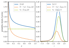
Figure 3: The true PDF s $f_{P}(p)$ and $f_{Z}(z)$ for $p$-values and $z$-scores from ScB described in Sec. VII. The two-groups model from Eq. (8) always holds, i.e., $f_{S}(s)$ is composed of a null and an alternative component. $f_{P|\mathrm{H}_{0}}\!(p)$ and $f_{Z|\mathrm{H}_{0}}\!(z)$ are known analytically. $\pi_{0}$ and $f_{P|\mathrm{H}_{1}}\!(p)$ and $f_{Z|\mathrm{H}_{1}}\!(z)$ are unknown. In general, the alternative component for one-sided $p$-values is a monotonically decreasing function. For one-sided $z$-scores, the alternative component exhibits a heavy left tail.

The lfdr can be computed on the basis of any local summary statistics which are i.i.d. under $\mathrm{H}_{0}$. Nevertheless, the local decision statistic plays an important role in lfdr estimation since it determines the shape of $f_{P}(p)$, as shown in Fig. 3.

We use $p$-values as local decision statistics. The domain of the $p$-values $\mathcal{F}=[0,1]$ is bounded and parametric models are used for $p$-value density estimation. The exact analytical form of $f_{P}(p)$ is unknown. However, if a sufficiently flexible parametric $p$-value PDF model is used, lfdr estimation based on $p$-values offers the following advantages. The $p$-values from sensors where $\mathrm{H}_{0}$ is in place are uniformly distributed. The $p$-values from sensors where $\mathrm{H}_{1}$ is in place are highly concentrated towards $0$. Hence, $f_{P|\mathrm{H}_{1}}\!(p)$ is a monotonically decreasing function and most of the mass of $f_{P}(p)$ is located in a subregion of $\mathcal{F}$ that contains the statistically significant (small) $p$-values. Additionally, $p$-value-based lfdr estimation allows for a simple way [45] to decompose estimate $\hat{f}_{P}(p)$ into the components of the two-groups model $\hat{\pi}_{0}f_{P|\mathrm{H}_{0}}\!(p)=\hat{\pi}_{0}$ and $\hat{f}_{P|\mathrm{H}_{1}}\!(p)$, $p\in\mathcal{F}=[0,1]$,

$$\hat{\pi}_{0}=\min\hat{f}_{P}(p),\qquad\hat{f}_{P|\mathrm{H}_{1}}\!(p)=\frac{\hat{f}_{P}(p)-\hat{\pi}_{0}}{1-\hat{\pi}_{0}}.$$ (9)

An alternate popular choice for local decision statistics are $z$-scores, for which a one-to-one mapping to $p$-values exists. The $z$-scores from sensor where $\mathrm{H}_{0}$ is in place follow a standard normal distribution. $z$-score-based lfdr estimators have been designed assuming a finite Gaussian mixture model [46] or an exponential family model [38, 29]. Non-parametric methods have been studied using kernel estimates [47] and, more recently, predictive recursion [39, 34, 48, 49]. We prefer $p$-values for the following reasons. The $z$-scores from sensors where $\mathrm{H}_{1}$ is in place lie in the tails of the $z$-score mixture PDF. Obtaining high tail-accuracy for an estimated PDF is extremely difficult. In addition, the decomposition of $\hat{f}_{Z}(z)$ into $\hat{\pi}_{0}f_{Z|\mathrm{H}_{0}}\!(z)$ and $(1-\hat{\pi}_{0})\hat{f}_{Z|\mathrm{H}_{1}}\!(z)$ is non-trivial.

The presumeably most popular parametric $p$-value PDF model is the beta-and-uniform mixture (BUM) model [45],

$${f}^{\text{BUM}}_{P}(p)={w}+(1-{w})\,\mathrm{beta}({\color[rgb]{0,0,0}p;}\,{a})={w}+(1-{w}){a}p^{{a}-1}.$$ (10)

Superscript BUM indicates the dependency on the BUM parameters ${w}\in[0,1]$ and ${a}\in(0,1)$. $\hat{f}^{\text{BUM}}_{P}(p)$ denotes the BUM model with the respective maximum likelihood estimator (MLE) $\hat{w}$ for $w$ and $\hat{a}$ for $a$. The BUM model exploits two known properties of $f_{P}(p)$, which are also apparent in Fig. 3. First, the uniform distribution under $\mathrm{H}_{0}$ is captured by the constant $w$. Second, $f_{P|\mathrm{H}_{1}}\!(p)$ is known to be monotonically decreasing. A single-parameter beta distribution decreases monotonically $\forall\,a\in(0,1)$. The BUM model is simple and has been applied successfully in a number of applications. However, it lacks flexibility due to its limited number of tuning parameters. Estimating $f_{P}(p)$ by $\hat{f}_{P}(p)=\hat{f}^{\text{BUM}}_{P}(p)$ leads to overly pessimistic lfdr estimates, as the simulations in Sec. VII underline. We introduce a more flexible model in Sec. IV.

IV The Proposed LFDR Estimator

In this section, we introduce a novel lfdr estimator. Our approach estimates lfdr’s from $p$-values. We propose the parametric probability model

$${f}^{\text{BM}}_{P}(p)=\sum_{l=1}^{L}{w}^{(l)}\,\mathrm{beta}\big{(}{\color[rgb]{0,0,0}p;}\,{a}^{(l)}\big{)},$$ (11)

a finite single-parameter beta distribution mixture (BM) with shape parameters ${a}^{(l)}\in\mathbb{R}_{>0}$ and mixture weights ${w}^{(l)}\in[0,1],\,\forall\,l\in[L]$ such that $\sum_{l=1}^{L}{w}^{(l)}=1$ and $L<\infty$. For ${a}^{(l)}<1$, ${a}^{(l)}=1$ and ${a}^{(l)}>1$, the $l$-th component $\mathrm{beta}({\color[rgb]{0,0,0}p;}\,{a}^{(l)})$ is monotonically decreasing, constant and monotonically increasing in $p\in[0,1]$, respectively. Due to the increased number of components, ${f}^{\text{BM}}_{P}(p)$ is more flexible than ${f}^{\text{BUM}}_{P}(p)$. Estimating its parameters is more involved than for the BUM model, since $2L-1$ model parameters are to be determined from the observations ${\color[rgb]{0,0,0}\mathcal{P}^{N}}=\{p_{1},\dots,p_{{\color[rgb]{0,0,0}N}}\}$. Closed-form MLE s for the parameters of mixture distributions are difficult to obtain. Instead, MLE s are commonly found iteratively by expectation-maximization (EM) [50], which is computationally expensive for larger model orders. Also, the parameter estimates are only locally optimal, which may result in poorly fitting models for non-convex likelihood functions. In this work, we target computationally light-weighted procedures suitable for large-scale sensor networks. Our approach bases upon the method of moments (MoM) that estimates model parameters by solving pre-defined equation systems.

IV-A The method of moments

The principle of moment-based parameter estimation [51, 52] is to match population and empirical moments. To this end, multivariate systems of moment equations are solved. The MoM is conceptionally simple, but also entails challenges. Its analytic complexity rapidly increases with the number of model parameters. In addition, empirical higher-order moments are prone to large variance [53]. Therefore, the sample size required to provide meaningful estimates grows exponentially in the number of model parameters [54]. As a consequence, the standard MoM is not well-suited to determining the parameters for Eq. (11).

The spectral method of moments (sMoM), a recent approach [55, 54], allows to determine the parameters of multivariate Gaussian mixtures from only the first three moments. Thus, sMoM avoids higher-order moments. In contrast to other work on the field of low-order moment-based parameter estimation, the method in [54] does not require a minimum distance between the locations of the mixture components to guarantee identifiability. This suits particularly well to this work, since we are dealing with $p$-values on the domain $\mathcal{F}=[0,1]$ and need to discriminate between mixture components that are located closely to one another. Combining the BM model and the sMoM provides a base for a computationally efficient $p$-value density estimator that we introduce in what follows.

IV-B Overview on the proposed method

We follow the traditional approach to lfdr estimation, which plugs estimates for $f_{P}(p)$ and $\pi_{0}$ into Eq. (5). Since we work with $p$-values, $\pi_{0}$ can be estimated as the maximum value of $f_{P}(p)$. Hence, we focus on the estimation of $f_{P}(p)$. We start from the assumption that the model in Eq. 11 holds for the PDF $f_{P}(p)$ of RV $P$ with realizations $\mathcal{P}^{N}=\{p_{1},\dots,p_{N}\}$. We then subdivide $\mathcal{P}^{N}$ into $M$ subsets of equal size $d$ and form $p$-value vectors $\mathbf{p}_{1},\dots,\mathbf{p}_{M}$. The $\mathbf{p}_{m},m\in[M]$ are observations of a $d$-dimensional random vector $\boldsymbol{p}=[\tilde{P}_{1},\dots,\tilde{P}_{d}]^{\top}$, where each $\tilde{P}_{i},i\in[d]$ represents the statistical behavior of a subset of all observed $p$-values. Due to the way that the $\mathbf{p}_{m}$ are obtained, there is a direct relation between the PDFs of $P$ and $\boldsymbol{p}$. Thus, the parametric multivariate PDF model for $\boldsymbol{p}$ follows directly from Eq. 11. The details are provided in Sec. IV-C. Then, we estimate the parameters of this multivariate model from the first three moments of $\boldsymbol{p}$. The empirical moments are computed using the observations $\mathbf{p}_{1},\dots,\mathbf{p}_{M}$. To this end, we exploit the one-to-one relations between the moments and the model parameters derived in Theorem 1 and Theorem 2 of Sec. IV-D. Finally, we again use the relation between the PDFs of $P$ and $\boldsymbol{p}$ to obtain the estimate of the univariate PDF of $P$ from the estimate for the multivariate PDF of $\boldsymbol{p}$. The entire procedure is presented in detail in Sec. IV-E.

IV-C The multivariate $p$-value model

Traditional statistical techniques would treat the input data ${\color[rgb]{0,0,0}\mathcal{P}^{N}}=\{p_{1},\dots,p_{{\color[rgb]{0,0,0}N}}\}$ as a single observation of an ${\color[rgb]{0,0,0}N}$-dimensional random vector with elements $P_{{\color[rgb]{0,0,0}n}},n\in[{\color[rgb]{0,0,0}N}]$. The identification of the regions associated with null hypothesis and alternative $\mathcal{H}_{0}$ and $\mathcal{H}_{1}$ based on a single observation of a high-dimensional random vector is fairly challenging. To perform spatial inference, we adopt the idea of learning from the experience of others [29] and treat ${\color[rgb]{0,0,0}\mathcal{P}^{N}}$ as ${\color[rgb]{0,0,0}N}$ realizations of the same scalar random variable $P\sim f_{P}(p)$. We first model the $p$-values as a $d$-dimensional random vector $\boldsymbol{p}$ instead of estimating $f_{P}(p)$ directly from ${\color[rgb]{0,0,0}\mathcal{P}^{N}}$. Then, we estimate its joint PDF $f_{\boldsymbol{p}}(\mathbf{p})$. Finally, we average over the $d$ marginals to obtain the univariate estimate $\hat{f}_{P}(p)$. Estimating a joint PDF appears intuitively more challenging. However, our multivariate $p$-value model enables fast and reliable estimation of $f_{P}(p)$, since it facilitates the application of the sMoM. To the best of our knowledge, this concept is entirely new to lfdr estimation.

In what follows, assume $P\sim f_{P}(p)={f}^{\text{BM}}_{P}(p)$. We divide the set of observations ${\color[rgb]{0,0,0}\mathcal{P}^{N}}=\{p_{1},\dots,p_{{\color[rgb]{0,0,0}N}}\}$ for random variable $P\sim{f}^{\text{BM}}_{P}(p)$ into $M$ distinct subsets $\mathcal{P}^{d}_{1},\dots,\mathcal{P}^{d}_{M}$ of equal size $d$, $M=\lfloor{\color[rgb]{0,0,0}N}/d\rfloor$. Any remaining $p$-values are not used for the PDF estimation. Next, arrange the elements of each $\mathcal{P}^{d}_{m}$ in no particular order into $M$ $d$-dimensional $p$-value vectors $\mathbf{p}_{m}\,\forall\,m\in[M]$. $\mathbf{p}_{1},\dots,\mathbf{p}_{M}$ are observations of the random vector $\boldsymbol{p}\sim f_{\boldsymbol{p}}(\mathbf{p})$, whose $i$-th entry be random variable $\tilde{P_{i}},i\in[d]$. Since $P\sim{f}^{\text{BM}}_{P}(p)$, the marginal distribution of each $\tilde{P_{i}}$ can be described without loss of generality by a $K$-component mixture

$$\tilde{P_{i}}\sim\sum_{k=1}^{K}{w}^{(k)}\mathrm{beta}\big{(}{\color[rgb]{0,0,0}p;}\,{a}^{(k)}_{i}\big{)},$$ (12)

with mixture proportion vector $\mathbf{w}=[{w}^{(1)},\dots,{w}^{(K)}]^{\top}$ such that $\sum_{k=1}^{K}{w}^{(k)}=1$ and shape parameters ${a}^{(k)}_{i}\in\mathbb{R}_{>0}$. The partitioning of ${\color[rgb]{0,0,0}\mathcal{P}^{N}}$ into $\mathcal{P}^{d}_{1},\dots,\mathcal{P}^{d}_{M}$ and the ordering of the entries within each $\mathbf{p}_{m}$, $m\in[M]$ must be found independently of the values $p_{{\color[rgb]{0,0,0}n}}$, ${\color[rgb]{0,0,0}n}\in[{\color[rgb]{0,0,0}N}]$. Then, the $\tilde{P_{i}}\,\forall\,i\in[d]$ are mutually independent random variables. Thus, $f_{\boldsymbol{p}}(\mathbf{p})$ is fully characterized by its marginals, which relate to ${f}^{\text{BM}}_{P}(p)$ through

$${f}^{\text{BM}}_{P}(p)=d^{-1}\sum_{k=1}^{K}{w}^{(k)}\sum_{i=1}^{d}\mathrm{beta}\big{(}{\color[rgb]{0,0,0}p;}\,{a}^{(k)}_{i}\big{)}.$$ (13)

Note, that the total number of mixture components $L$ from Eq. (11) is then $L=K\cdot d$.

Based on the result in [56, Chapter 24], the first two cumulants, mean $\kappa_{1_{i}}^{(k)}$ and variance $\kappa_{2_{i}}^{(k)}$, of the $i$-th marginal’s $k$-th component are found $\forall\,i\in[d],\,\forall\,k\in[K]$, as

$$\kappa_{1_{i}}^{(k)}=\frac{{a}^{(k)}_{i}}{{a}^{(k)}_{i}+1},\quad\kappa_{2_{i}}^{(k)}=\frac{{a}^{(k)}_{i}}{{a}^{(k)}_{i}+2}-\Bigg{(}\frac{{a}^{(k)}_{i}}{{a}^{(k)}_{i}+1}\Bigg{)}^{2}.$$ (14)

The third-order cumulant, is

$$\kappa_{3_{i}}^{(k)}\!=\!\frac{{a}^{(k)}_{i}}{{a}^{(k)}_{i}\!+3}-\frac{3{a}^{(k)}_{i}}{\big{(}{a}^{(k)}_{i}\!+2\big{)}}\frac{{a}^{(k)}_{i}}{\big{(}{a}^{(k)}_{i}\!+1\big{)}}+2\Bigg{(}\frac{{a}^{(k)}_{i}}{{a}^{(k)}_{i}\!+1}\Bigg{)}^{3}\!.$$ (15)

Additionally, denote the $k$-th mixture component mean vector by $\boldsymbol{\kappa}_{1}^{(k)}=\big{[}\kappa_{1_{1}}^{(k)},\dots,\kappa_{1_{d}}^{(k)}\big{]}^{\top}$ and the $k$-th component vector of third-order cumulants by $\boldsymbol{\kappa}_{3}^{(k)}=\big{[}\kappa_{3_{1}}^{(k)},\dots,\kappa_{3_{d}}^{(k)}\big{]}^{\top}$ for all $k\in[K]$. We also define the averages across mixture components, $\overline{\boldsymbol{\kappa}_{1}}=[\overline{\kappa_{1_{1}}},\dots,\overline{\kappa_{1_{d}}}]^{\top}=\sum_{k=1}^{K}{w}^{(k)}\boldsymbol{\kappa}_{1}^{(k)}$, and $\overline{\boldsymbol{\kappa}_{3}}=[\overline{\kappa_{3_{1}}},\dots,\overline{\kappa_{3_{d}}}]^{\top}=\sum_{k=1}^{K}{w}^{(k)}\boldsymbol{\kappa}_{3}^{(k)}$. Since the $\tilde{P_{i}}\,\forall\,i\in[d]$ are independently distributed, the $k$-th component’s $d\times d$ covariance matrix $\mathbf{\Sigma}^{(k)}$ is diagonal with the $i$-th entry $\kappa_{2_{i}}^{(k)}$. The $d\times d$ mixture covariance matrix is $\mathbf{\Sigma}=\operatorname{E}\left[(\boldsymbol{p}-\overline{\boldsymbol{\kappa}_{1}})(\boldsymbol{p}-\overline{\boldsymbol{\kappa}_{1}})^{\top}\right]$.

To conclude this section, we formulate the following assumption on the $p$-values.

Assumption 1 (Similar component variances).

The marginal variances of the $k$-th mixture component are similar, such that they can be treated as approximately equivalent across the marginals, i.e., $\kappa_{2}^{(k)}\approx\kappa_{2_{i}}^{(k)}\,\forall\,i\in[d]$, $k\in[K]$.

In other words, for a certain $m\in[M]$, the entries of $\mathbf{p}_{m}$ can be treated as observations of random variables with approximately equivalent variances.

Our simulation results in Sec. VII confirm that Assumption 1 is fairly mild. We conducted a large number of numerical experiments with very diverse underlying spatial signals. Our proposed lfdr estimator was always able to find a subset size $M<{\color[rgb]{0,0,0}N}$ and a number of mixture components $K<d$ for which the $p$-value subsets $\mathcal{P}^{d}_{m}$ and vectors $\mathbf{p}_{m}$, $m\in[M]$ were formed such that Assumption 1 holds for each mixture component $k\in[K]$. Hence, the $\mathbf{p}_{m},m\in[M]$, can be divided into $K$ groups such that joint PDF of the $p$-value vectors in each group is described by mixture component $k$. For illustration purposes, consider that the subsets $\mathcal{P}^{d}_{m}$ are formed based on spatial proximity, i.e., each $\mathcal{P}^{d}_{m}$ is composed of $p$-values from $d$ neighboring locations. For those subsets containing exclusively $p$-values from locations ${\color[rgb]{0,0,0}n}\in\mathcal{H}_{0}$, the statistical properties of each element are similar by design. Due to the assumed spatial smoothness of spatial phenomena, also the $p$-values obtained at close-by locations ${\color[rgb]{0,0,0}n}\in\mathcal{H}_{1}$ have similar statistical properties.

Under Assumption 1, the $k$-th mixture component covariance matrix is $\mathbf{\Sigma}^{(k)}\approx\kappa_{2}^{(k)}\mathbf{I}_{d\times d}$, where $\mathbf{I}_{d\times d}$ is the $d\times d$ identity matrix. The average variance over mixture components is $\overline{\kappa_{2}}\approx\sum_{k=1}^{K}{w}^{(k)}\kappa_{2}^{(k)}$.

IV-D The spectral method of moments

The spectral method of moments was formulated for multivariate spherically Gaussian distributed data in [54]. Their approach builds on the relation between the population moments and the model parameters, namely, the mixture weights, means and variances. In this section, we formulate similar relations for the $p$-value vectors, given that they follow the model from Eq. (12) and fulfill Assumption 1. We first extend [54, Theorem 2] such that it fits to our proposed data model.

Theorem 1 (Relation of mixture model parameters to spectral quantities).

For a $d\times 1$ random vector $\boldsymbol{p}{\color[rgb]{0,0,0}=[\tilde{P_{1}},\dots,\tilde{P_{d}}]^{\top}}$ with joint PDF $f_{\boldsymbol{p}}(\mathbf{p})$ and the marginals of $\tilde{P_{1}},\dots,\tilde{P_{d}}$ are distributed as defined in Eq. (12), under Assumption 1, the beta distribution shape parameters ${a}^{(k)}_{i}\,\forall\,i\in[d]$ and mixture component weights ${w}^{(k)}\,\forall\,k\in[K]$ can be expressed by ${a}^{(k)}_{i}=\frac{\kappa_{1_{i}}^{(k)}}{1-\kappa_{1_{i}}^{(k)}}$ and $\mathbf{w}=\Big{[}\boldsymbol{\kappa}_{1}^{(1)},\dots,\boldsymbol{\kappa}_{1}^{(K)}\Big{]}^{\dagger}\overline{\boldsymbol{\kappa}_{1}}=\Big{[}{w}^{(1)},\dots,{w}^{(K)}\Big{]}^{\top}$ with

$$\boldsymbol{\kappa}_{1}^{(k)}=\frac{\lambda^{(k)}}{\boldsymbol{\eta}^{\top}\mathbf{B}\mathbf{v}^{(k)}}\mathbf{B}\mathbf{v}^{(k)},$$ (16)

if $K<d$, ${w}^{(k)}>0,\,\forall\,k\in[K]$ and the $k$-th mixture component mean vectors $\boldsymbol{\kappa}_{1}^{(k)}\,\forall\,k\in[K]$ are linearly independent. Here, $\boldsymbol{\eta}=[\eta_{1},\dots,\eta_{d}]^{\top}$ is a vector chosen uniformly at random from the unit sphere in $\mathbb{R}^{d}$, $\big{(}\lambda^{(k)},\mathbf{v}^{(k)}\big{)},\,k\in[K]$ are the (eigenvalue, eigenvector) pairs of a $K\times K$ matrix $\mathbf{W}^{\top}{\mathbf{M}}_{3}({\boldsymbol{\eta}})\mathbf{W}$. The projection matrices $\mathbf{B}={\mathbf{U}}\big{(}{\mathbf{U}}^{\top}\mathbf{M}_{2}{\mathbf{U}}\big{)}^{\frac{1}{2}}\in\mathbb{R}^{K\times d}$ and $\mathbf{W}={\mathbf{U}}\big{(}{\mathbf{U}}^{\top}\mathbf{M}_{2}{\mathbf{U}}\big{)}^{\dagger\frac{1}{2}}\in\mathbb{R}^{d\times K}$ are based on the matrix of left singular vectors ${\mathbf{U}}\in\mathbb{R}^{d\times K}$ of the thin singular value decomposition (SVD) of $\mathbf{M}_{2}={\mathbf{U}}\mathbf{S}\mathbf{R}^{\top}$. In addition, $\mathbf{M}_{2},{\mathbf{M}}_{3}({\boldsymbol{\eta}})\in\mathbb{R}^{d\times d}$ and $\underline{\mathbf{M}}_{3}\in\mathbb{R}^{d\times d\times d}$ such that

$$\mathbf{M}_{2} =\sum_{k=1}^{K}{w}^{(k)}\boldsymbol{\kappa}_{1}^{(k)}\circ\boldsymbol{\kappa}_{1}^{(k)},$$ (17)

$${\mathbf{M}}_{3}({\boldsymbol{\eta}}) =\sum_{i_{1}=1}^{d}\sum_{i_{2}=1}^{d}\sum_{i_{3}=1}^{d}\big{[}\underline{\mathbf{M}}_{3}\big{]}_{i_{1},i_{2},i_{3}}[\boldsymbol{\eta}]_{i_{3}}\mathbf{e}_{i_{1}}\!\circ\mathbf{e}_{i_{2}},$$ (18)

$$\underline{\mathbf{M}}_{3} =\sum_{k=1}^{K}\big{(}{w}^{(k)}\boldsymbol{\kappa}_{1}^{(k)}\circ\boldsymbol{\kappa}_{1}^{(k)}\circ\boldsymbol{\kappa}_{1}^{(k)}\big{)},$$ (19)

with $\mathbf{e}_{i}$ a $d\times 1$ vector of $d-1$ zeros and $1$ as its $i$-th entry. $\circ$ is the outer product.

Proof.

${a}^{(k)}_{i}=\frac{\kappa_{1_{i}}^{(k)}}{1-\kappa_{1_{i}}^{(k)}}$ follows from Eq. (14). The relations for the mixture component means $\boldsymbol{\kappa}_{1}^{(k)}$, $k\in[K]$ and the mixture proportion vector $\mathbf{w}$ result directly from the proof of [54, Theorem 2]. Note, that $\mathbf{B}\mathbf{B}^{\top}=\mathbf{M}_{2}$ and $\mathbf{W}\mathbf{W}^{\top}=\mathbf{M}_{2}^{-1}$, which implies that $\mathbf{W}^{\top}{\mathbf{M}}_{3}({\boldsymbol{\eta}})\mathbf{W}=\mathbf{R}^{\top}\mathbf{D}(\boldsymbol{\eta})\mathbf{R}$ is diagonalizable along the lines of $\mathbf{M}_{\text{GMM}}(\boldsymbol{\eta})$ in [54, Theorem 2] by a diagonal matrix $\mathbf{D}(\boldsymbol{\eta})\in\mathbb{R}^{K\times K}$ with diagonal entries $\lambda^{(k)}=\boldsymbol{\eta}^{\top}\boldsymbol{\kappa}_{1}^{(k)},k\in[K]$. ∎

The relations established in Theorem 1 allow to estimate the mixture model by means of its parameters $\boldsymbol{\kappa}_{1}^{(k)}$ and $\mathbf{w}$, since $\overline{\boldsymbol{\kappa}_{1}}$, $\mathbf{M}_{2}$, and $\underline{\mathbf{M}}_{3}$ enable a one-to-one mapping between the model parameters and the observable population moments. In particular, $\overline{\boldsymbol{\kappa}_{1}}=\operatorname{E}\left[\boldsymbol{p}\right]$ is the first moment of $\boldsymbol{p}$, whereas $\mathbf{M}_{2}$ and $\underline{\mathbf{M}}_{3}$ are related to the second and third moments $\operatorname{E}\left[\boldsymbol{p}\circ\boldsymbol{p}\right]$ and $\operatorname{E}\left[\boldsymbol{p}\circ\boldsymbol{p}\circ\boldsymbol{p}\right]$ of $\boldsymbol{p}$. The exact relationships are derived in Theorem 2.

Theorem 2 (Relation of spectral to observable quantities).

Under the assumptions in Theorem 1, the average variance over mixture components $\overline{\kappa_{2}}=\sum_{k=1}^{K}{w}^{(k)}\kappa_{2}^{(k)}$ is the smallest eigenvalue of the population covariance matrix $\mathbf{\Sigma}$. With $\mathbf{v}\in\mathbb{R}^{d}$ any unit-norm eigenvector of eigenvalue $\overline{\kappa_{2}}$, we find

$$\mathbf{M}_{2} =\operatorname{E}\left[\boldsymbol{p}\circ\boldsymbol{p}\right]-\overline{\kappa_{2}}\mathbf{I}_{d\times d},$$ (20)

$$\underline{\mathbf{M}}_{3} =\tilde{\underline{\mathbf{M}}}_{3}-\underline{\mathbf{M}}_{3}^{\Delta},$$ (21)

where the observable $\tilde{\underline{\mathbf{M}}}_{3}$ and the difference $\underline{\mathbf{M}}_{3}^{\Delta}$ to the non-observable $\underline{\mathbf{M}}_{3}$ are

$$\begin{split}\tilde{\underline{\mathbf{M}}}_{3}&=\operatorname{E}\left[\boldsymbol{p}\circ\boldsymbol{p}\circ\boldsymbol{p}\right]-\sum_{i=1}^{d}\big{(}\tilde{\mathbf{m}}_{1}\circ\mathbf{e}_{i}\circ\mathbf{e}_{i}\\ &\qquad+\mathbf{e}_{i}\circ\tilde{\mathbf{m}}_{1}\circ\mathbf{e}_{i}+\mathbf{e}_{i}\circ\mathbf{e}_{i}\circ\tilde{\mathbf{m}}_{1}\big{)},\end{split}$$ (22)

$$\underline{\mathbf{M}}_{3}^{\Delta} =\underline{\mathbf{M}}_{3}^{\Delta_{3}}-\underline{\mathbf{M}}_{3}^{\Delta_{1}},$$ (23)

with third-order tensors $\tilde{\underline{\mathbf{M}}}_{3},\underline{\mathbf{M}}_{3}^{\Delta_{3}},\underline{\mathbf{M}}_{3}^{\Delta_{1}}\in\mathbb{R}^{d\times d\times d}$, $d\times 1$ vector $\tilde{\mathbf{m}}_{1}=\mathbf{m}_{1}+\mathbf{m}_{1}^{\Delta}\in\mathbb{R}^{d}$,

$$\tilde{\mathbf{m}}_{1} =\operatorname{E}\left[\boldsymbol{p}\Big{(}\mathbf{v}^{\top}\big{(}\boldsymbol{p}-\overline{\boldsymbol{\kappa}_{1}}\big{)}\Big{)}^{2}\right],\quad\mathbf{m}_{1}^{\Delta}=\vphantom{\sum_{k=1}^{K}}\mathbf{v}\odot\mathbf{v}\odot\overline{\boldsymbol{\kappa}_{3}}.$$ (24)

$\odot$ denotes the Hadamard product and

$$\underline{\mathbf{M}}_{3}^{\Delta_{3}}=\sum_{i=1}^{d} \Big{(}\overline{\kappa_{3_{i}}}\,\mathbf{e}_{i}\circ\mathbf{e}_{i}\circ\mathbf{e}_{i}\Big{)}$$ (25)

$$\begin{split}\underline{\mathbf{M}}_{3}^{\Delta_{1}}=\sum_{i=1}^{d}&\Big{(}\mathbf{m}_{1}^{\Delta}\circ\mathbf{e}_{i}\circ\mathbf{e}_{i}\\ &+\mathbf{e}_{i}\circ\mathbf{m}_{1}^{\Delta}\circ\mathbf{e}_{i}+\mathbf{e}_{i}\circ\mathbf{e}_{i}\circ\mathbf{m}_{1}^{\Delta}\Big{)}.\end{split}$$ (26)

$\overline{\boldsymbol{\kappa}_{3}}=\big{[}\overline{\kappa_{3_{1}}},\dots,\overline{\kappa_{3_{d}}}\big{]}^{\top}$ is the vector composed of the $d$ marginals’ mean third cumulants, i.e., Eq. (15) $\forall\,i\in[d]$ averaged over the $K$ mixture components.

Proof.

See Appendix A. ∎

The first and second population moments $\overline{\boldsymbol{\kappa}_{1}}$ and $\operatorname{E}\left[\boldsymbol{p}\circ\boldsymbol{p}\right]$, the population covariance matrix $\mathbf{\Sigma}$ and consequently also $\overline{\kappa_{2}}$, $\mathbf{v}$ and $\mathbf{M}_{2}$ can be found using consistent sample estimates of the moments and covariance. ${\mathbf{M}}_{3}({\boldsymbol{\eta}})$ cannot be estimated directly, since only $\tilde{\underline{\mathbf{M}}}_{3}$ depends exclusively on sample moments, but not $\underline{\mathbf{M}}_{3}^{\Delta}$. However, we show in Appendix B that $\tilde{{\mathbf{M}}}_{3}(\boldsymbol{\eta})=\sum_{i_{1}=1}^{d}\sum_{i_{2}=1}^{d}\sum_{i_{3}=1}^{d}\big{[}\tilde{\underline{\mathbf{M}}}_{3}\big{]}_{i_{1},i_{2},i_{3}}[\boldsymbol{\eta}]_{i_{3}}\mathbf{e}_{i_{1}}\!\circ\mathbf{e}_{i_{2}}$ is a sufficiently good approximation of ${\mathbf{M}}_{3}({\boldsymbol{\eta}})$ for estimating the $p$-value mixture density. $\tilde{{\mathbf{M}}}_{3}(\boldsymbol{\eta})$ is observable. In the following section, we exploit these relations to estimate the component first central moments $\boldsymbol{\kappa}_{1}^{(k)}$ and the model parameters ${a}^{(k)}_{i}$, ${w}^{(k)}$ $\,\forall\,k\in[K],\,\forall\,i\in[d]$ for Eq. (13).

IV-E The lfdr-sMoM estimator

The proposed method is summarized in Alg. 1. It partitions the $p$-values into subsets, estimates the parameters for the joint PDF of the resulting $p$-value vectors and determines $\hat{f}_{P}(p)=\hat{f}^{\text{BM}}_{P}(p)$ from Eq. (13). The density fit is repeated several times for $G$ different $p$-value vectors, increasing subset sizes $d=2,3,\dots$ and increasing model orders $K<d$. $M\cdot d=\lfloor N/d\rfloor\cdot d$ $p$-values are used for the density fit if $N/d$ is not an integer. If the distinct subsets $\mathcal{P}^{d}_{m}\subset{\color[rgb]{0,0,0}\mathcal{P}^{N}}$ are fixed, because they are formed based on fixed covariate information like spatial proximity, we randomly rearrange the elements $G$ times within each $p$-value vector for different runs. Selecting $G=10$ created sufficient flexibility to find $p$-value vectors that yield sufficiently accurate density model estimates in all considered scenarios. The lfdr’s are estimated using $\hat{f}_{P}(p)$, Eq. (9) and Eq. (7). The goodness of fit is assessed by the value $\ell^{\ast}$ of a difference measure between $\hat{f}_{P}(p)$ and the data. $\ell^{\ast}$ is initialized with a large value, to ensure that the algorithm finds a solution. The best solution has been found, if additional degrees of freedom do not lead to a better fit.

The parameters of the $p$-value vector mixture density are estimated by Alg. 2, which determines the right side of Eq. (16) from the sample moments. In Line 1, the data is split into two distinct sets of equal size. If $M$ is odd, we drop one $\mathbf{p}_{m}$. The sample moment-based estimates $\hat{{\mathbf{M}}}_{2}$ for $\mathbf{M}_{2}$ and $\hat{\tilde{{\mathbf{M}}}}_{3}({\boldsymbol{\eta}})$ for $\tilde{{\mathbf{M}}}_{3}(\boldsymbol{\eta})$ are multiplied during the estimation process. Hence, they must be computed from different data to guarantee their independence. The sample covariance matrix estimates $\hat{\mathbf{\Sigma}}_{\mathcal{S}}$ in Line 3 are full rank, but Line 5 reduces the rank to its assumed value $K$. $\hat{\tilde{\underline{\mathbf{M}}}}_{3}$ is determined in Lines 6 and 7. Lines 8 to 13 are dedicated to the estimation of the eigenvector, eigenvalue pairs $\big{(}\lambda^{(k)},\mathbf{v}^{(k)}\big{)}$ for Eq. (16). We generate $U$ different vectors $\boldsymbol{\eta}_{u}$ and select the best run in Alg. 1 to fulfill Lemma 1 given in Appendix B. We found a value as low as $U=10$ to provide satisfying results.

Algorithm 1 The proposed algorithm lfdr-sMoM

Input: ${\color[rgb]{0,0,0}\mathcal{P}^{N}}=\{p_{1},\dots,p_{{\color[rgb]{0,0,0}N}}\}$, $G$, $\mathrm{d}(\cdot,\cdot)$, $U$
      Output: $\hat{\mathrm{lfdr}}_{1},\dots,\hat{\mathrm{lfdr}}_{{\color[rgb]{0,0,0}N}}$

1:Step 1: Estimation of $f_{P}(p)$

2:Initialize $\ell^{\ast}$ as the largest possible number

3:Compute the histogram $\mathrm{hist}(\mathcal{P}^{Q})$ for the data in ${\color[rgb]{0,0,0}\mathcal{P}^{N}}$

4:for $d\in\mathbb{N}_{\geq 2}$ do

5:     Divide ${\color[rgb]{0,0,0}\mathcal{P}^{N}}$ into subsets $\mathcal{P}^{d}_{m}$, $m\in[M]$

6:     for $g\in[G]$ do

7:         [l]Form vectors $\mathbf{p}_{m}\in\mathbb{R}^{d},\forall\,m\in[M]$, by random

8:ordering of the elements in $\mathcal{P}^{d}_{m}$

9:         Define $\mathcal{P}^{d\times M}=\big{\{}\mathbf{p}_{m}\in\mathbb{R}^{d}\,|\,m\in[M]\big{\}}$, $\ell^{d}=\infty$

10:         for $K\leq d$ do

11:              [l]Obtain $U$ sets of parameters $\hat{w}^{(k)}_{u}$, $\hat{a}^{(k)}_{i,u},$

12:$\forall\,k\in[K],\forall\,i\in[d],\forall\,u\in[U]$ via Alg. 2

13:              Find $\hat{f}_{P}^{u}(p)$ for $\hat{w}^{(k)}_{u},\hat{a}^{(k)}_{i,u}$ and Eq. (13) $u\in[U]$

14:              Select $u^{\ast}\!=\!\mathrm{argmin}_{u}\big{(}\mathrm{d}(\mathrm{hist}(\mathcal{P}^{Q}),\hat{f}_{P}^{u}(p))\big{)}$

15:              if $\mathrm{d}(\mathrm{hist}(\mathcal{P}^{Q}),\hat{f}_{P}^{u^{\ast}}(p))<\ell^{d}$ then

16:                  $\ell^{d}=\mathrm{d}(\mathrm{hist}(\mathcal{P}^{Q}),\hat{f}_{P}^{u^{\ast}}(p))$

17:                  if $\ell^{d}\leq\ell^{\ast}$ then

18:                       $\ell^{\ast}=\ell^{d},\hat{f}_{P}(p)=\hat{f}_{P}^{u^{\ast}}(p)$, $d^{\ast}=d$                   

19:              else break.                             

20:     if $d^{\ast}\neq d$ then break.      

21:Step 2: Estimation of $\pi_{0}$ and $f_{P|\mathrm{H}_{1}}\!(p)$

22:Compute $\hat{\pi}_{0}=\min\big{(}\hat{f}_{P}(p)\big{)}$

23:Compute $\hat{f}_{P|\mathrm{H}_{1}}\!(p)=\big{(}1-\hat{\pi}_{0}\big{)}^{-1}(\hat{f}_{P}(p)-\hat{\pi}_{0}\big{)}$

24:Determine $\hat{\mathrm{lfdr}}_{{\color[rgb]{0,0,0}n}},\forall\,{\color[rgb]{0,0,0}n}\in[{\color[rgb]{0,0,0}N}]$ from Eq. (7)

Algorithm 2 Mixture model parameter estimation

Input: $\mathcal{P}^{d\times M}=\big{\{}\mathbf{p}_{m}\in\mathbb{R}^{d}\,|\,m=1,\dots,M\big{\}}$, $K$
      Output: $\hat{\mathbf{w}}_{u}\in\mathbb{R}^{K}$, $\hat{a}^{(k)}_{i,u},\forall\,i\in[d],\forall\,k\in[K],\forall\,u\in[U]$

1:Randomly split $\mathcal{P}^{d\times M}$ into $\big{\{}\!\mathcal{Q},\mathcal{R}\,\big{|}\,|\mathcal{Q}|=|\mathcal{R}|,\mathcal{Q}\,\cap\,\mathcal{R}\!=\!\emptyset\!\big{\}}$

2:Compute ${\hat{\overline{\boldsymbol{\kappa}}}_{1_{\mathcal{S}}}}={|\mathcal{S}|}^{-1}\sum_{\mathbf{p}\in\mathcal{S}}\mathbf{p},\mathcal{S}=\mathcal{Q},\mathcal{R}$

3:Find $\hat{\mathbf{\Sigma}}_{\mathcal{S}}={|\mathcal{S}|}^{-1}\big{(}\sum_{\mathbf{p}\in\mathcal{S}}\mathbf{p}\mathbf{p}^{\top}\big{)}-{\hat{\overline{\boldsymbol{\kappa}}}_{1_{\mathcal{S}}}}{\hat{\overline{\boldsymbol{\kappa}}}_{1_{\mathcal{S}}}}^{\top}$

4:Determine $\hat{\overline{\kappa}}_{2_{\mathcal{S}}}$, the smallest eigenvalue of $\hat{\mathbf{\Sigma}}_{\mathcal{S}}$ and $\hat{\mathbf{v}}_{\mathcal{S}}$, its corresponding eigenvector

5:Compute the best rank-$K$ estimate of $\mathbf{M}_{2}$,

$$\hat{{\mathbf{M}}}_{2}=\arg\min_{\mathbf{X}\in\mathbb{R}^{d\times d}|\mathrm{rank}(\mathbf{X})\leq K}\big{|}\big{|}\hat{\mathbf{\Sigma}}_{\mathcal{Q}}-\mathbf{X}\big{|}\big{|}_{2}.$$

6:Find $\hat{\tilde{\mathbf{m}}}_{1_{\mathcal{S}}}=|\mathcal{S}|^{-1}$ $\sum_{\mathbf{p}\in\mathcal{S}}\mathbf{p}\Big{(}\hat{\mathbf{v}}_{\mathcal{S}}\big{(}\mathbf{p}-{\hat{\overline{\boldsymbol{\kappa}}}_{1_{\mathcal{S}}}}\big{)}^{2}\Big{)}$

7:Compute $\hat{\tilde{\underline{\mathbf{M}}}}_{3}=|\mathcal{R}|^{-1}\Big{(}\sum_{\mathbf{p}\in\mathcal{R}}\mathbf{p}\circ\mathbf{p}\circ\mathbf{p}\Big{)}-\sum_{i=1}^{d}\Big{(}\hat{\tilde{\mathbf{m}}}_{1_{\mathcal{R}}}\circ\mathbf{e}_{i}\circ\mathbf{e}_{i}+\mathbf{e}_{i}\circ\hat{\tilde{\mathbf{m}}}_{1_{\mathcal{R}}}\circ\mathbf{e}_{i}+\mathbf{e}_{i}\circ\mathbf{e}_{i}\circ\hat{\tilde{\mathbf{m}}}_{1_{\mathcal{R}}}\Big{)}$

8:Find $\hat{{\mathbf{U}}}\in\mathbb{R}^{d\times K}$, the left singular vectors of $\hat{{\mathbf{M}}}_{2}$

9:Compute $\hat{\mathbf{W}}=\hat{{\mathbf{U}}}\big{(}\hat{{\mathbf{U}}}^{\top}\hat{{\mathbf{M}}}_{2}\hat{{\mathbf{U}}}\big{)}^{\dagger\frac{1}{2}}\in\mathbb{R}^{d\times K}$ and $\hat{\mathbf{B}}=\hat{{\mathbf{U}}}\big{(}\hat{{\mathbf{U}}}^{\top}\hat{{\mathbf{M}}}_{2}\hat{{\mathbf{U}}}\big{)}^{\frac{1}{2}}\in\mathbb{R}^{K\times d}$

10:for $u\in[U]$ do

11:     Select $\boldsymbol{\eta}_{u}$ uniformly at random from the $\mathbb{R}^{d}$ unit sphere

12:     Find $\hat{\mathbf{W}}^{\top}\!\hat{\tilde{{\mathbf{M}}}}_{3}({\boldsymbol{\eta}_{u}})\hat{\mathbf{W}}\!\in\!\mathbb{R}^{K\!\times\!K}$ $\forall\,k,l\!\in[K]$,

$$\Big{[}\hat{\mathbf{W}}^{\top}\hat{\tilde{{\mathbf{M}}}}_{3}({\boldsymbol{\eta}_{u}})\hat{\mathbf{W}}\Big{]}_{k,l}\!=\!\sum_{h,i,j\in[d]}\![\hat{\mathbf{W}}]_{h,k}[\hat{\mathbf{W}}]_{i,l}[\boldsymbol{\eta}_{u}]_{j}\Big{[}\hat{\tilde{\underline{\mathbf{M}}}}_{3}\Big{]}_{h,i,j}$$

13:     [l]Determine the (eigenvalue, eigenvector) pairs

14:$\Big{(}\hat{\lambda}^{(k)}_{u},\hat{\mathbf{v}}^{(k)}_{u}\Big{)},k\in[K]$, of $\hat{\mathbf{W}}^{\top}\hat{\tilde{{\mathbf{M}}}}_{3}({\boldsymbol{\eta}_{u}})\hat{\mathbf{W}}$

15:     Compute $\hat{\boldsymbol{\kappa}}_{1}^{(k)}=\Big{(}\boldsymbol{\eta}_{{\color[rgb]{0,0,0}u}}^{\top}\hat{\mathbf{B}}\hat{\mathbf{v}}^{(k)}_{{\color[rgb]{0,0,0}u}}\Big{)}^{-1}\hat{\lambda}^{(k)}_{{\color[rgb]{0,0,0}u}}\hat{\mathbf{B}}\hat{\mathbf{v}}^{(k)}_{{\color[rgb]{0,0,0}u}}$, $k\in[K]$

16:     Determine $\hat{\mathbf{w}}_{u}=\Big{[}\hat{\boldsymbol{\kappa}}_{1}^{(1)},\dots,\hat{\boldsymbol{\kappa}}_{1}^{(K)}\Big{]}^{\dagger}{\hat{\overline{\boldsymbol{\kappa}}}_{1_{\mathcal{Q}}}}$

17:     Obtain $\hat{a}^{(k)}_{i,u}=\frac{\hat{\boldsymbol{\kappa}}_{1}^{(k)}}{1-\hat{\boldsymbol{\kappa}}_{1}^{(k)}},\forall\,i\in[d],\forall\,k\in[K]$

The best density fit is determined based on a difference measure $\mathrm{d}(\hat{f}_{P}^{u}(p),\mathrm{hist}(\mathcal{P}^{Q}))$ between model estimates $\hat{f}_{P}^{u}(p)$ and the histogram of the observed data. We ran Alg. 1 with some of the most popular measures for quantifying closeness based on probability densities and distributions. We found Alg. 1 to be robust w.r.t. the selected difference measure in terms of FDR control. We observed that using empirical distribution function (EDF)-based distances such as the Wasserstein (WS) or Kolmogorov-Smirnov (KS) distance resulted in slightly higher detection power for very small $\pi_{0}$ than PDF-based divergences, such as the Kullback-Leibler (KL) or the Jensen–Shannon (JS) divergence. Thus, we stick to EDF distances.

Our method inherently avoids overfitting. The model order is limited by the number of elements per subset, $K<d$. Hence, increasing $d$ adds flexibility and reduces the mismatch $\underline{\mathbf{M}}_{3}^{\Delta}$ between the observable and non-observable theoretical third-order moment dependent terms. Contrarily, increasing $d$ decreases the validity of Assumption 1, i.e., equal variance among the multivariate mixture components. In addition, an increase in $d$ reduces the accuracy of the model parameter estimates due to the decrease in sample size $M=\lfloor{\color[rgb]{0,0,0}N}/d\rfloor$ and increase in the number of parameters to be estimated.

V Interpolation of local false discovery rates

In this section, we discuss how to determine the decision statistics between the spatially sparse sensor locations. Like in Fig. 4, sensors are typically positioned at a subset of locations $\{\mathbf{c}_{n}\}_{n\in N},N\leq Q$. These report local $p$-values $\mathcal{P}^{N}=\{p_{1},\dots,p_{N}\}$ to the FC. The FC computes sensor-level lfdr estimates $\hat{\mathrm{lfdr}}_{n},\forall\,n\in[N]$ using lfdr-sMoM. The lfdr’s are interpolated to estimate the lfdr’s $\hat{\mathrm{lfdr}}_{q}$ at locations $\{\mathbf{c}_{q}\}$ between sensors, $N<q\leq Q$. The lfdr’s are unknown deterministic quantities. Thus, we deploy a deterministic interpolation method. Radial basis function (RBF) interpolation is an advanced mesh-free method to reconstruct an unknown deterministic function from observed data [57, 58]. The function value at a location of interest is calculated as a weighted sum of smooth basis functions whose value depends on the location’s distance to the sampling locations. RBF is well suited to the problem at hand: The sensors can be located at arbitrary locations within the observation area. The interpolant is stable also for a large number of sensors [59]. Finally, it produces a smooth interpolant, whose properties depend on the deployed radial basis function. The properties of thin-plate splines (TPS) [60] fit particularly well to our central assumption of spatial smoothness, i.e., that the null and alternative regions are formed of locally continuous sub-regions with quick transitions in between. TPS finds values in between sampling points under a constraint on the energy of the interpolant. Thus, it produces a very smooth interpolant with sharp transitions [61] in between sensor locations where the lfdr’s differ significantly. In addition, TPS RBF s does not require ad-hoc tuning of additional parameters. This would be necessary, if other popular basis functions, such as the Gaussian or multiquadric were used.

The interpolated lfdr’s are calculated as

$$\hat{\mathrm{lfdr}}_{q}=\sum_{n=1}^{N}\alpha_{n}\varphi(r_{{n},{q}}),\qquad q\in[Q],$$ (27)

where $r_{{n},{q}}=||\mathbf{c}_{n}-\mathbf{c}_{q}||_{2}$ is the Euclidean distance between sensor and location, $\varphi(r_{{n},{q}})=r_{{n},{q}}^{2}\ln(r_{{n},{q}})$ is the TPS RBF and the weights $\alpha_{n}\in\mathbb{R}$ are determined based on the estimated sensor lfdr’s and locations by solving [58, Chapter 8.3]

$$\begin{bmatrix}\varphi(r_{{1},{1}})&\cdots&\varphi(r_{{1},{N}})\\ \vdots&\ddots&\vdots\\ \varphi(r_{{N},{1}})&\cdots&\varphi(r_{{N},{1}})\end{bmatrix}\begin{bmatrix}\alpha_{1}\\ \vdots\\ \alpha_{N}\end{bmatrix}$$

$$\qquad\qquad\qquad+{\color[rgb]{0,0,0}\begin{bmatrix}1&c_{\text{x},1}&c_{\text{y},1}\\ \vdots&\vdots&\vdots\\ 1&c_{\text{x},N}&c_{\text{y},N}\end{bmatrix}\begin{bmatrix}\beta_{1}\\ \beta_{2}\\ \beta_{3}\end{bmatrix}}=\begin{bmatrix}\hat{\mathrm{lfdr}}_{1}\\ \vdots\\ \hat{\mathrm{lfdr}}_{N}\end{bmatrix},$$

with regularization parameters such that $\sum_{n=1}^{N}\alpha_{n}=0$, $\sum_{n=1}^{N}\alpha_{n}c_{\text{x},n}=0$, and $\sum_{n=1}^{N}\alpha_{n}c_{\text{y},n}=0$.

VI Communication Cost and Power Consumption

In practice, the $p$-values have to be quantized before the transmission over the wireless communication channel. Only few bits will suffice so that no significant performance loss is experienced. In this section, we quantitatively analyze the total network communication cost $\mathrm{CC}_{N}$ and communication-related power consumption $\mathrm{PC}_{N}$ for a WSN of size $N$ w.r.t. the number of bits that each sensor is allowed to transmit. The $\mathrm{CC}_{N}$ and $\mathrm{PC}_{N}$ are expressed quantitatively as

$$\mathrm{CC}_{N} =\sum_{n=1}^{N}\big{(}\mathrm{CF}+\mathrm{CB}(B)\big{)}\cdot\mathrm{NP}_{n},$$ (28)

$$\mathrm{PC}_{N} =\sum_{n=1}^{N}\big{(}\mathrm{NP}_{n}\cdot\mathrm{CT}(B)\big{)},$$ (29)

where $\mathrm{NT}_{n}$ is the number of packets that sensor $n\in[N]$ transmits, i.e., the number of transmissions per sensor. For simplicity, we assume that each transmission of sensor $n$ is equally costly. The total cost per transmission depends on $\mathrm{CF}$ which represents the payload-independent cost of the deployed transmission protocol and the cost $\mathrm{CB}(B)$ that depends on the number of payload bits $B$. $\mathrm{CT}(B)$ is the power consumption per transmitted packet with $B$ payload bits. For simplicity, we assume that all costs and the number of information-carrying bits are identical for all sensors. Transmitting data is the most power-intensive task for the sensors in our WSN. Simple local computations to determine the soft decision statistics consume much less power.

$\mathrm{CC}_{N}$ and $\mathrm{PC}_{N}$ of our proposed method with $\mathrm{NP}_{n}=1\,\forall\,n\in[N]$ is considerably different from a fully centralized approach where each local measurement is communicated to the FC. For example, assume that each sensor records a total number of $256$ local measurements. If the $B$ is the same for the $p$-values and the raw measurements, a centralized approach consumes $256$ times more communication bandwidth and power than the proposed approach.

Consider the following practical example for the relevance of the number of payload bits. A simple and very important internet protocol (IP) is the user datagram protocol (UDP). An empty, i.e., no payload, UDP packet consumes $\mathrm{CF}=28$ bytes. In addition, UDP transmits bytes instead of single bits, i.e., $\mathrm{CC}_{N}$ does not grow linear in the number of payload bits $B$, bit is constant for $B=1$ to $B=8$. Hence, if one sends $1$, $4$ or $8$ bits of payload data, the frame structure overhead is well above $90\%$ of the total communication cost and there is no difference if $1$, $4$ or $8$ bits of information is transmitted.

The best way to reduce the communication cost and power consumption is to limit the total number of transmissions in the WSN. This could be achieved by imposing communication constraints and transmitting only informative data as is done in censoring [62, 63]. Our simulation results demonstrate that the proposed method also works if $p$-values above a certain threshold $\lambda\leq 1$ are censored, i.e., if a sensor $n\in[N]$ may only transmit its quantized $p$-value $p^{\text{q}}_{n}$ if $p^{\text{q}}_{n}>\lambda$. No censoring occurs if $\lambda=1$.

VII Simulation Results

(a) Detection pattern

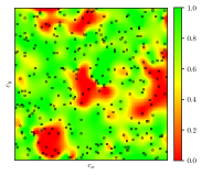
(b) Interpolated lfdr’s

Figure 4: Example for ScB, Cnfg. 2. In a), the FDR threshold is set to $\alpha_{\operatorname{FDR}}=10\%$. Green, red and gray indicate true, false and missed discoveries. Boxes mark sensor locations. The interpolated lfdr’s of b) are discussed in Sec. VII-C.

We evaluate the performance of our proposed spatial inference method on simulated radio frequency electromagnetic field data. The observed signals are simulated by the nonuniform sampling method from [64], which models the propagation of radio waves in a 2D spatial area with path loss and shadow fading [40]. The observations are subject to additive white Gaussian sensor noise. If the power of the received signal is below the noise floor, this sensor is classified as located in the true null region $\mathcal{H}_{0}$. If no sensor is present at a grid point, this grid point is assigned to $\mathcal{H}_{0}$ if the signal level of the field at this grid point is so low that it would be below the noise floor of a reference sensor placed at this location. In our simulations, we alter the sensor noise power for different scenarios to obtain different sizes $|\mathcal{H}_{1}|=1-\pi_{0}$ of the regions of interesting, different or anomalous behavior.

For simplicity, the sensor $p$-values are computed from signal energies. This facilitates the analysis of the results, since its known distributions under null and alternative hypotheses allow for benchmarking the lfdr estimation techniques against the true lfdr’s. Also, it offers a simple way to simulate a heterogeneous sensor network by alternating the number of measurements $T$ at different nodes. In practice, any type of sufficient test statistic could be deployed at the sensor level.

We evaluated our method for a variety of simulated propagating radio wave fields in different environments and sensor network configurations. We discuss the results for three scenarios typical for radio frequency sensing. The monitored area is discretized by a grid of $100\times 100$ spatial elements for all scenarios and the results are averaged over $200$ independent Monte Carlo runs, unless stated otherwise. The sources are placed at random locations, i.e., the fraction $\pi_{0}$ of grid points in the null region varies slightly from run to run.

ScA: Five sources located in a suburban environment covering on average $1-\pi_{0}\approx 55\%$ of grid points.

ScB: Eight sources located in a suburban environment covering on average $1-\pi_{0}\approx 34\%$ of grid points.

ScC: Two sources in a suburban environment covering on average $1-\pi_{0}\approx 10\%$ of grid points.

ScC is particularly challenging, regardless of the deployed method. Only a small proportion of test statistics provide information on the shape of the alternative component $f_{P|\mathrm{H}_{1}}\!(p)$.

We investigate four different sensor network configurations.

Cnfg. 1: $N=10\,000$ identical sensors with $T=256$. Decisions are only made at sensor locations, i.e., no interpolation of decision statistics. This is the classic MHT problem.

Cnfg. 2: $N=300$ identical sensors with $T=256$, homogeneously distributed across the monitored area. The tests at the sensors are based on local summary statistics, but in between sensors, the lfdr’s are interpolated.

Cnfg. 3: $N_{1}=170$ sensors with $T_{1}=256$, $N=80$ sensors with $T_{2}=512$ and $N_{3}=50$ sensors $T_{3}=1024$, all types homogeneously distributed across the monitored area. Decisions in between sensors base upon interpolated lfdr’s.

Cnfg. 4: $N=2\,000$ identical sensors with $T=256$, homogeneously distributed across the monitored area. The decisions at the sensors are based on local summary statistics, but in between sensors, the lfdr’s are interpolated.

Competitors: To the best of our knowledge, there exist no other methods to identify the regions of anomaly with guarantees on error probabilities or the FDR when sensors are located at a sparse but arbitrary subset of grid points. In [15], the authors consider the classic MHT problem for WSNs, hence, we can compare our proposed lfdr-based inference approach to their distributed Benjamini-Hochberg (dBH) procedure [15] for a WSN in Cnfg. 1. In addition, we compare the proposed lfdr-based inference approach when different lfdr-estimators are used. We compare our proposed lfdr-sMoM to a variety of popular lfdr estimators. We deploy the classic BUM model-based MLE approach from [45]. We also show results obtained with Lindsey’s method (LM) as proposed by Efron [29]. LM which approximates the $z$-score PDF by an exponential family model, fitted to the data using Poisson regression. In addition, predictive recursion (PR) [49, 39] is applied, which computes the alternative $z$-score PDF by estimating the density of the mean shift of $z$-scores from locations in $\mathcal{H}_{1}$. Predictive recursion has recently [34, 48, 31] gained considerable attention in lfdr estimation, due to its high accuracy and comparably low computation time. Our implementation of PR follows [34, Appendix A]. Finally, we include a standard Gaussian mixture model (GMM). We do not consider methods whose computational complexity prevents scaling to large-scale sensor networks, as kernel density lfdr estimators [47].

VII-A The classic multiple hypothesis testing problem

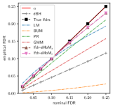
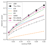
(a) ScA

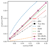
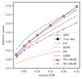
(b) ScB

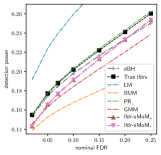
(c) ScC

Figure 6: FDR and detection power for all scenarios and a sensor network composed of $N=10\,000$ nodes. Decisions are only made at the sensor locations (Cnfg. 1). The FDR is strictly controlled for all scenarios with all estimators except LM. Among those for which the FDR is controlled, the proposed lfdr-sMoM yields the highest power in ScA, ScB. In ScC, where $\mathcal{H}_{1}$ contains only a small fraction of all nodes, the power with PR is slightly higher.

The results for Cnfg. 1 are shown in Fig. 6. dBH works well in ScC where $\pi_{0}\approx 10\%$ is small. When $\pi_{0}$ gets larger, dBH lacks detection power. The results for the different lfdr estimators with the proposed lfdr-based spatial inference method are ambiguous. We benchmark by the detection results obtained when using the (in practice unknown) true lfdr’s. A higher detection power than with the true lfdr’s can only be achieved if the respective lfdr estimator leads to a violation of the nominal FDR level. LM faces stability issues due to the heavy one-sided tail of $f_{Z}(z)$ when the relative size of the true null region $\pi_{0}=|\mathcal{H}_{0}|/N$ increases. With all other lfdr estimators, the considered nominal FDR levels are met. For the proposed lfdr estimator, we show results for two variants. For lfdr-sMoM _s, the $p$-value vectors are formed by subdividing the grid into square tiles of spatially close grid points. For lfdr-sMoM _r, the $\{p_{n}\}_{n\in[N]}$ are randomly partitioned into subsets.

The results underline that our proposed multivariate $p$-value vector probability density model is very flexible. Even if the $p$-value subsets are formed at random, the method finds a parametrization such that the individual components have equal variance. This confirms that Assumption 1 can be relaxed in practice. For the remainder of this section, we stick to the conceptually simpler random partitioning and label results obtained with randomly formed $p$-value vectors by lfdr-sMoM.

For the traditional BUM estimator, the lfdr is controlled but the detection power is low in all scenarios, as for GMM for larger interesting regions. PR performs best by a small margin when the relative size of the alternative region is very small (ScC), but with our proposed estimator, the largest detection power is achieved in ScB and ScA. Thus, lfdr-sMoM provides the best or very close to the best results for all considered scenarios.

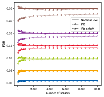
(a) FDR

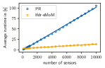
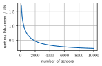
(b) Execution time

Figure 7: FDR s and run times with increasing sensor network size for lfdr-sMoM vs. the best competitor (PR) for ScB.

VII-B Computational demands as the network size increases

In Fig. 7, we compare the best competitor, PR, to our proposed method for different sizes of the sensor network $N$ and $1\,000$ Monte Carlo (MC) runs. We obtained almost identical results for all scenarios and hence show only those for ScB. Again, inference is only performed at the sensor locations. Both, the proposed lfdr-sMoM and PR, are subject to transient effects when the number of nodes is small. This was to be expected, as fitting a complicated distribution model with such a low number of data points is challenging. Yet, the obtained FDR s are close to the nominal level also for the smallest considered network sizes $N$. As $N$ grows, the nominal and empirical FDR for lfdr-sMoM coincide almost perfectly. Hence, lfdr-sMoM is more efficient in exploiting all permitted false positives than PR, which results in a larger detection power (plot not shown due to space limitations). The comparison of the average execution time per Monte Carlo run in Fig. 7(b) illustrates that the proposed estimator is considerably faster than PR as $N$ increases. The upper plot shows that the execution time for both methods grows approximately linearly. For a small number of sensors, the runtimes of lfdr-sMoM and PR are almost identical, but the former scales significantly better for larger sensor networks. At $N=10\,000$, lfdr-sMoM is more than five times faster. Both methods were run in Python 3.8.3 on an AMD Ryzen 9 3900X 12-Core CPU. We conclude that while lfdr-sMoM often provides the highest detection power, it also outperforms its strongest competitor significantly in terms of computation time for growing $N$.

VII-C Spatial interpolation of lfdr’s

It is of high interest to find the boundaries of the regions associated with interesting, anomalous or different behavior. Our proposed lfdr-based spatial inference approach determines the values in between the sensor locations by spatial interpolation. This allows for segmenting the observation area into $\mathcal{H}_{0}$ and $\mathcal{H}_{1}$ with FDR control.

An exemplary map of interpolated lfdr’s with $N=300$ identical sensors (Confg. 2). is shown in Fig. 4, along the detection pattern for the most commonly used [29] nominal FDR level $\alpha_{\operatorname{FDR}}=0.1$. In Tab. I, we present the numerical FDR s and detection powers obtained by interpolating the estimated sensor lfdr’s. Note, that the interpolation step of the proposed inference approach is independent of the selected lfdr estimator, see also Fig. 2.

The FDR is controlled at the nominal level, except for the very small $\alpha_{\operatorname{FDR}}=0.01$. This nominal level is so small, that even the slightest interpolation error can lead to its violation. For higher, more realistic nominal FDR levels, the FDR is strictly controlled. In this example, sensors are located at only $3\%$ of all grid points. The lfdr’s are interpolated at the remaining $97\%$. These results strongly indicate that the interpolation of lfdr’s is a powerful tool to decide between $\mathrm{H}_{0}$ and $\mathrm{H}_{1}$ at locations where no sensor is present and local summary statistics are not available.

In Cnfg. 3, we considered a heterogeneous sensor network composed of multiple types of sensors with different individual detection capabilities due to varying sensor noise levels. The results in Tab. II verify the applicability of our method to heterogeneous sensor networks, i.e., to accommodate various types of sensors into the inference process.

Table I: ScB in Cnfg. 2. The columns indicate different nominal FDR levels. The similarity in the empirical values of FDR and detection power obtained when using lfdr-sMoM or in practice the unavailable true lfdr’s as base for the interpolation underline the effectiveness of our method.

	$\alpha_{\operatorname{FDR}}$	$.01$	$.05$	$.1$	$.15$	$.2$	$.25$	$.3$
FDR	True	$\mathit{.020}$	$\mathit{.030}$	$\mathit{.05}$	$\mathit{.08}$	$\mathit{.12}$	$\mathit{.17}$	$\mathit{.22}$
	lfdr-sMoM	$.029$	$.043$	$.07$	$.10$	$.15$	$.19$	$.24$
Power	True	$\mathit{.10}$	$\mathit{.18}$	$\mathit{.25}$	$\mathit{.33}$	$\mathit{.40}$	$\mathit{.47}$	$\mathit{.55}$
	lfdr-sMoM	$.11$	$.19$	$.26$	$.34$	$.41$	$.48$	$.55$

Table II: ScB in Cnfg. 3. The columns indicate different nominal FDR levels. Also for a heterogeneous sensor network, the FDR is controlled except for the very small $\alpha_{\operatorname{FDR}}=.01$.

	$\alpha_{\operatorname{FDR}}$	$.01$	$.05$	$.1$	$.15$	$.2$	$.25$	$.3$
FDR	lfdr-sMoM	$.023$	$.039$	$.07$	$.11$	$.15$	$.20$	$.25$
Power	lfdr-sMoM	$.15$	$.24$	$.33$	$.42$	$.49$	$.56$	$.63$

VII-D Quantized $p$-values

In practice, the $p$-values have to be quantized prior to the transmission over the wireless communication channel. In this section, we demonstrate that the performance of our proposed spatial inference approach with lfdr-sMoM is close to the optimum when $p$-values are quantized with few bits. Since little support for the null hypothesis is indicated by small $p$-values, quantizers that provide a higher resolution for smaller $p$-values and lower resolution for larger $p$-values are expected to be more efficient than for example uniform quantizers. For the purpose of illustration, we use the following ad-hoc $p$-value quantizer. Divide the $p$-value domain $[0,1]$ with $B$ bits into $2^{B}$ intervals of width

$$w_{i}=\frac{i}{\sum_{j=1}^{2^{B}}j},\qquad i=1,\dots,2^{B}.$$

The left and right edges of the $i$-th quantization interval are

$$\mathrm{le}_{i}=\frac{\sum_{j=1}^{i-1}j}{\sum_{j=1}^{2^{B}}j},\quad\mathrm{re}_{i}=\frac{\sum_{j=1}^{i}j}{\sum_{j=1}^{2^{B}}j},$$

respectively. Fig. 9 shows the empirical FDR and detection power in Cnfg. 1, i.e., with a sensor located at each of the $10\,000$ grid points. We use $B\in[3,5,8]$ bits. Only the results with the true (unknown) lfdr’s, the proposed lfdr estimator lfdr-sMoM and PR are shown.

The results underline that our proposed inference method works well with quantized $p$-values with only a negligible performance loss compared to unquantized case. We first analyze the performance with the true lfdr’s, i.e., independent of the influence of an lfdr estimator. As $B$ increases, the detection power rises. Saturation is reached quickly, $B=5$ bits provide nearly identical performance as in Fig. 6 with unquantized $p$-values. Only for the very challenging ScC and nominal FDR levels $\alpha<.15$, using more than $B=5$ bits yields a noticeable increase in detection power. With the proposed lfdr-sMoM, the results are very similar: As few as $B=5$ bits are enough for close to nominal performance at the commonly used nominal FDR level $\alpha=.1$ in ScA and ScB. In the very challenging ScC, a few bits are needed, but $B=8$ yields very good results. Again, a very small $B$ may lead to reduced detection power, but FDR control is strictly maintained with lfdr-sMoM. This is significantly different with PR. With PR, the nominal FDR level $\alpha$ is violated if $B$ is too small. Even for $B=8$, the nominal FDR level is violated in ScB and ScC. We obtained similar results for other $N$ and interpolated lfdr’s. While these results confirm that our proposed method is applicable if the sensors report $p$-values that are quantized using few bits, these results also make a strong case in favor of the proposed lfdr estimator lfdr-sMoM for spatial inference with WSNs.

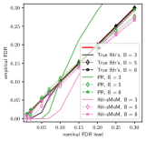
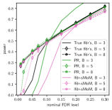
(a) ScA

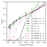
(b) ScB

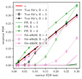
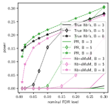
(c) ScC

Figure 9: FDR and detection power for all scenarios and a sensor network composed of $N=10\,000$ nodes and quantized $p$-values. Decisions are only made at the sensor locations (Cnfg. 1). lfdr-based spatial inference works also with $p$-values that are quantized using few bits. The FDR is strictly controlled with proposed lfdr estimator lfdr-sMoM.

We conclude the simulation results with a brief outlook on the effect that censoring [62, 63] has on the proposed approach. As discussed in Sec. VI, allowing only sensors with quantized $p$-values $\leq\lambda$ to transmit can reduce the communication cost and power consumption considerably. In Fig. 10, the empirical FDR and detection power for ScA and Cnfg. 4, i.e., $N=2\,000$ sensors are shown. The same quantizer as in the previous paragraph is used with $B=5$ bits. We compare the lfdr-based spatial inference approach with true lfdr’s and lfdr’s estimated by our proposed lfdr-sMoM. If $\lambda=1$, no censoring occurs. There is no performance difference for the considered values of $\lambda$ with the true lfdr’s. However, this may be different for even smaller $\lambda$ or other scenarios, where $\lambda$ would censor $p$-values that would lead to a discovery at the FC. The performance with lfdr-sMoM is close to optimum at standard nominal FDR levels for all $\lambda$. This is remarkable, as only about $1/3$ of all sensors transmit their $p$-values to the FC for $\lambda=.12$. This offers great savings in communication cost and power consumption. The analytical derivation of the censoring regions remains a future research topic.

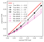
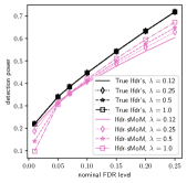
Figure 10: FDR and detection power for ScA, Cnfg. 4 and different censoring thresholds $\lambda$. Censoring has little impact on the detection power while offering great potential to saving on communication cost and power consumption.

VIII The inclusion of domain-specific knowledge

While we kept this work general to maintain its applicability to a wide area of practical problems, extending the procedure to explicitly account for the particular nature of the observed physical phenomenon, such as electromagnetic spectrum, air quality or agricultural fields appears promising. This could further increase the detection power. Due to the modular nature of the proposed inference method, improving the individual blocks in Fig. 2 can lead to improved results without the necessity to come up with an entirely new approach. For example, one can exploit the spatial smoothness assumption not only in the estimation of the probability models, but also to increase the detection power. One possible approach is to replace the lfdr with the contextual lfdr (clfdr). The difference is that $\pi_{0}$ depends on the sensor location in the clfdr. Its location-dependent value can be estimated from the data. One could plug in an novel or existing method [32, 31] into Eq. (5). Alternatively, one could include a penalty term into RBF interpolation to spatially smoothen the interpolant [57]. Choosing the value of this parameter is non-trivial and should be done in an application-dependent manner.

IX Summary

We proposed a novel lfdr-based inference method for detecting interesting, different or anomalous regions of an observed physical phenomenon. Our approach provides statistical performance guarantees in terms of false positives. The proposed method facilitates solving real-world spatial inference problems in which distributed heterogeneous large-scale sensor networks observe spatial phenomena. The sensors communicate with a fusion center or cloud only in a limited fashion. This saves battery and ensures a long sensor life-span. Moreover, the method estimates the local false discovery rates in between the actual sensor locations. Consequently, the proposed method allows for identifying spatial regions where alternative hypotheses are in place while strictly controlling the FDR. The decision making takes place at the fusion center or in the cloud. In addition, we proposed a novel approach to estimating the local false discovery based on the spectral method of moments. It outperforms existing methods in terms of detection power and runtime in a variety of scenarios. It is considerably faster than state-of-the-art methods and yields close-to-optimum results for $p$-values that are quantized using few bits. This is important for inference with wireless sensor networks, since the sensors communicate their information over the wireless communication channel. The performance was evaluated by an application to spatially varying radio frequency waves. The code to reproduce the results is available on https://github.com/mgoelz95/lfdr-sMoM.

Appendix A Proof of Theorem 2

We establish the one-to-one relations between the first three population moments $\operatorname{E}\left[\boldsymbol{p}\right],\operatorname{E}\left[\boldsymbol{p}\circ\boldsymbol{p}\right],\operatorname{E}\left[\boldsymbol{p}\circ\boldsymbol{p}\circ\boldsymbol{p}\right]$ and the model parameter-dependent operators $\mathbf{M}_{2}\in\mathbb{R}^{d\times d}$, $\underline{\mathbf{M}}_{3}\in\mathbb{R}^{d\times d\times d}$, which are given in Eq. (20) and Eq. (21). Since the sample moments are consistent estimates of the population moments, Theorem 1 enables model parameter estimation based on the sample moments.

A-A Proof of Eq. (20)

Under Assumption 1 with $d>K$, the covariance matrix $\mathbf{\Sigma}\in\mathbb{R}^{d\times d}$ can be written as

$$\mathbf{\Sigma} =\operatorname{E}\left[(\boldsymbol{p}-\overline{\boldsymbol{\kappa}_{1}})\circ(\boldsymbol{p}-\overline{\boldsymbol{\kappa}_{1}})\right]$$

$$=\overline{\kappa_{2}}\mathbf{I}_{d\times d}+\sum_{k=1}^{K}{w}^{(k)}\Big{(}\boldsymbol{\kappa}_{1}^{(k)}-\overline{\boldsymbol{\kappa}_{1}}\Big{)}\circ\Big{(}\boldsymbol{\kappa}_{1}^{(k)}-\overline{\boldsymbol{\kappa}_{1}}\Big{)},$$ (30)

where $\sum_{k=1}^{K}{w}^{(k)}\Big{(}\boldsymbol{\kappa}_{1}^{(k)}-\overline{\boldsymbol{\kappa}_{1}}\Big{)}\circ\Big{(}\boldsymbol{\kappa}_{1}^{(k)}-\overline{\boldsymbol{\kappa}_{1}}\Big{)}$ is a $d\times d$ matrix of rank $K-1$. Consequently, the $d-(K-1)$ smallest eigenvalues of $\mathbf{\Sigma}$ are all equal to $\overline{\kappa_{2}}$. $\mathbf{v}\in\mathbb{R}^{d}$ is any of the unit norm eigenvectors corresponding to $\overline{\kappa_{2}}$. The derivation for Eq. (30) in the proof of [54, Theorem 1] applies also to our data model. Thus, also

$$\mathbf{M}_{2} =\operatorname{E}\left[\boldsymbol{p}\circ\boldsymbol{p}\right]-\overline{\kappa_{2}}\mathbf{I}_{d\times d}=\sum_{k=1}^{K}{w}^{(k)}\boldsymbol{\kappa}_{1}^{(k)}\circ\boldsymbol{\kappa}_{1}^{(k)}$$

holds and relates the observable second population moment $\operatorname{E}\left[\boldsymbol{p}\circ\boldsymbol{p}\right]$ to the model parameters.

A-B Proof of Eq. (21)

We now proof the relation $\underline{\mathbf{M}}_{3}=\tilde{\underline{\mathbf{M}}}_{3}-\underline{\mathbf{M}}_{3}^{\Delta}$ between the observable $\tilde{\underline{\mathbf{M}}}_{3}$ and non-observable $\underline{\mathbf{M}}_{3}$. Random vector $\boldsymbol{p}\in\mathbb{R}^{d}$ is assumed to follow a $d$-variate, $K$-component mixture model. It can hence be described by $\boldsymbol{p}=\boldsymbol{p}^{(\mathsf{k})}$, where $\mathsf{k}\in[K]$ is a discrete random variable for the mixture component index taking value $\mathsf{k}=k$ with probability ${w}^{(k)}\in[0,1]$ and $\sum_{k=1}^{K}{w}^{(k)}=1$. Let $\boldsymbol{q}^{(\mathsf{k})}=\boldsymbol{p}^{(\mathsf{k})}-\boldsymbol{\kappa}_{1}^{(\mathsf{k})}$ denote the centered data random vector and conditioned on $\mathsf{k}=k$, $\boldsymbol{q}^{(k)}=\boldsymbol{p}^{(k)}-\boldsymbol{\kappa}_{1}^{(k)}$. This implies $\operatorname{E}\left[\boldsymbol{q}^{(k)}\right]=\mathbf{0}_{d}$. Since $\boldsymbol{q}\in\mathbb{R}^{d}$, its $i$-th marginal is $q_{i}^{(k)}$, $i\in[d]$, and the marginal variances are $\operatorname{E}\left[{q_{i}^{(k)}}^{2}\right]=\kappa_{2}^{(k)}\,\forall\,k\in[K]$ under Assumption 1. The third order central moments are $\operatorname{E}\left[{q_{i}^{(k)}}^{3}\right]=\kappa_{3_{i}}^{(k)}$.

The third order population moment tensor $\operatorname{E}\left[\boldsymbol{p}\circ\boldsymbol{p}\circ\boldsymbol{p}\right]$ is

$$\operatorname{E}\left[\boldsymbol{p}\circ\boldsymbol{p}\circ\boldsymbol{p}\right]$$

$$=\sum_{k=1}^{K}{w}^{(k)}\bigg{(}\!\operatorname{E}\left[\Big{(}\!\boldsymbol{\kappa}_{1}^{(k)}\!+\!\boldsymbol{q}^{(k)}\!\Big{)}\!\circ\!\Big{(}\!\boldsymbol{\kappa}_{1}^{(k)}\!+\!\boldsymbol{q}^{(k)}\!\Big{)}\!\circ\!\Big{(}\!\boldsymbol{\kappa}_{1}^{(k)}\!+\!\boldsymbol{q}^{(k)}\!\Big{)}\right]\!\bigg{)}$$

$$=\sum_{k=1}^{K}\!{w}^{(k)}\!\bigg{(}\!\operatorname{E}\left[\boldsymbol{\kappa}_{1}^{(k)}\!\circ\boldsymbol{\kappa}_{1}^{(k)}\!\circ\boldsymbol{\kappa}_{1}^{(k)}\right]+\operatorname{E}\left[\boldsymbol{\kappa}_{1}^{(k)}\!\circ\boldsymbol{q}^{(k)}\circ\boldsymbol{q}^{(k)}\right]$$

$$\qquad\qquad\quad+\!\operatorname{E}\left[\boldsymbol{q}^{(k)}\circ\boldsymbol{\kappa}_{1}^{(k)}\!\circ\boldsymbol{q}^{(k)}\right]\!+\!\operatorname{E}\left[\boldsymbol{q}^{(k)}\circ\boldsymbol{q}^{(k)}\circ\boldsymbol{\kappa}_{1}^{(k)}\right]$$

$$\qquad\qquad\quad+\!\operatorname{E}\left[\boldsymbol{q}^{(k)}\circ\boldsymbol{q}^{(k)}\circ\boldsymbol{q}^{(k)}\right]\!\bigg{)}$$

$$=\sum_{k=1}^{K}\!{w}^{(k)}\!\bigg{(}\!\boldsymbol{\kappa}_{1}^{(k)}\!\circ\boldsymbol{\kappa}_{1}^{(k)}\!\circ\boldsymbol{\kappa}_{1}^{(k)}\!+\!\sum_{i=1}^{d}\Big{(}\boldsymbol{\kappa}_{1}^{(k)}\kappa_{2}^{(k)}\circ\mathbf{e}_{i}\circ\mathbf{e}_{i}$$

$$\qquad\qquad\quad+\mathbf{e}_{i}\circ\boldsymbol{\kappa}_{1}^{(k)}\kappa_{2}^{(k)}\circ\mathbf{e}_{i}+\mathbf{e}_{i}\circ\mathbf{e}_{i}\circ\boldsymbol{\kappa}_{1}^{(k)}\kappa_{2}^{(k)}$$

$$\qquad\qquad\quad+\kappa_{3_{i}}^{(k)}\mathbf{e}_{i}\!\circ\!\mathbf{e}_{i}\!\circ\!\mathbf{e}_{i}\Big{)}\bigg{)}$$

$$=\underline{\mathbf{M}}_{3}+\underline{\mathbf{M}}_{3}^{\Delta_{3}}+\sum_{i=1}^{d}\bigg{(}\sum_{k=1}^{K}{w}^{(k)}\Big{(}\boldsymbol{\kappa}_{1}^{(k)}\kappa_{2}^{(k)}\circ\mathbf{e}_{i}\circ\mathbf{e}_{i}$$

$$\qquad\quad+\mathbf{e}_{i}\circ\boldsymbol{\kappa}_{1}^{(k)}\kappa_{2}^{(k)}\circ\mathbf{e}_{i}+\mathbf{e}_{i}\circ\mathbf{e}_{i}\circ\boldsymbol{\kappa}_{1}^{(k)}\kappa_{2}^{(k)}\Big{)}\bigg{)}.$$ (31)

The definitions of $\tilde{\underline{\mathbf{M}}}_{3},\underline{\mathbf{M}}_{3}^{\Delta_{3}}\in\mathbb{R}^{d\times d\times d}$ are provided in Eq. (19) and Eq. (25). We proceed with $\tilde{\mathbf{m}}_{1}\in\mathbb{R}^{d}$,

$$\tilde{\mathbf{m}}_{1} =\operatorname{E}\left[\boldsymbol{p}\Big{(}\mathbf{v}^{\top}\big{(}\boldsymbol{p}-\overline{\boldsymbol{\kappa}_{1}}\big{)}\Big{)}^{2}\right]$$

$$=\sum_{k=1}^{K}{w}^{(k)}\operatorname{E}\left[\boldsymbol{p}^{(k)}\Big{(}\mathbf{v}^{\top}\big{(}\boldsymbol{p}^{(k)}-\overline{\boldsymbol{\kappa}_{1}}\big{)}^{2}\Big{)}\right]$$

$$=\sum_{k=1}^{K}{w}^{(k)}\operatorname{E}\left[\bigg{(}\boldsymbol{\kappa}_{1}^{(k)}+\boldsymbol{q}^{(k)}\bigg{)}\bigg{(}\mathbf{v}^{\top}\Big{(}\boldsymbol{\kappa}_{1}^{(k)}-\overline{\boldsymbol{\kappa}_{1}}+\boldsymbol{q}^{(k)}\Big{)}\bigg{)}^{2}\right]$$

$$=\sum_{k=1}^{K}{w}^{(k)}\operatorname{E}\left[\Big{(}\boldsymbol{\kappa}_{1}^{(k)}+\boldsymbol{q}^{(k)}\Big{)}\Big{(}\mathbf{v}^{\top}\boldsymbol{q}^{(k)}\Big{)}^{2}\right]$$

$$=\sum_{k=1}^{K}{w}^{(k)}\bigg{(}\operatorname{E}\left[\boldsymbol{\kappa}_{1}^{(k)}\Big{(}\mathbf{v}^{\top}\boldsymbol{q}^{(k)}\Big{)}^{2}\right]+\operatorname{E}\left[\boldsymbol{q}^{(k)}\Big{(}\mathbf{v}^{\top}\boldsymbol{q}^{(k)}\Big{)}^{2}\right]\bigg{)}$$

$$=\sum_{k=1}^{K}{w}^{(k)}\Big{(}\boldsymbol{\kappa}_{1}^{(k)}\kappa_{2}^{(k)}+\mathbf{v}\odot\mathbf{v}\odot\boldsymbol{\kappa}_{3}^{(k)}\Big{)}.$$ (32)

The transition from line 3 to 4 in Eq. (32) uses the property that $\mathbf{v}$ lies in the null space of ${w}^{(k)}\Big{(}\boldsymbol{\kappa}_{1}^{(k)}-\overline{\boldsymbol{\kappa}_{1}}\Big{)}\circ\Big{(}\boldsymbol{\kappa}_{1}^{(k)}-\overline{\boldsymbol{\kappa}_{1}}\Big{)}$. With $\operatorname{E}\left[q_{i_{1}}^{(k)}q_{i_{2}}^{(k)}\right]=0$ if $i_{1}\neq i_{2}$ due to the diagonal covariance matrix, the first addend in line 6 follows from line 5 by

$$\operatorname{E}\left[\boldsymbol{\kappa}_{1}^{(k)}\Big{(}\mathbf{v}^{\top}\boldsymbol{q}^{(k)}\Big{)}^{2}\right]=\boldsymbol{\kappa}_{1}^{(k)}\Bigg{(}\!\operatorname{E}\left[\sum_{i=1}^{d}\bigg{(}v_{i}^{2}{q_{i}^{(k)}}^{2}\bigg{)}\right]\!$$

$$\qquad+\sum_{i_{1}=1}^{d}\sum_{i_{2}=i_{1}+1}^{d}\!2\operatorname{E}\left[q_{i_{1}}^{(k)}q_{i_{2}}^{(k)}\right]v_{i_{1}}v_{i_{2}}\!\Bigg{)}.$$

For the second addend in Eq. (32),

$$\leavevmode\nobreak\ =\boldsymbol{\kappa}_{1}^{(k)}\sum_{i=1}^{d}v_{i}^{2}\operatorname{E}\left[{q_{i}^{(k)}}^{2}\right]=\boldsymbol{\kappa}_{1}^{(k)}\sum_{i=1}^{d}v_{i}^{2}\kappa_{2}^{(k)}=\boldsymbol{\kappa}_{1}^{(k)}\kappa_{2}^{(k)},$$

$$\operatorname{E}\left[\boldsymbol{q}^{(k)}\Big{(}\mathbf{v}^{\top}\boldsymbol{q}^{(k)}\Big{)}^{2}\right]=\operatorname{E}\left[\boldsymbol{q}^{(k)}\sum_{i=1}^{d}\Big{(}v_{i}^{2}{q_{i}^{(k)}}^{2}\Big{)}\right]$$

$$\qquad+\operatorname{E}\left[\boldsymbol{q}^{(k)}\sum_{i_{1}=1}^{d}\sum_{i_{2}=i_{1}+1}^{d}\big{(}2q_{i_{1}}^{(k)}q_{i_{2}}^{(k)}v_{i_{1}}v_{i_{2}}\big{)}\right].$$

For the $j$-th entry, $j\in[d]$, of vector $\operatorname{E}\left[\boldsymbol{q}^{(k)}\Big{(}\mathbf{v}^{\top}\boldsymbol{q}^{(k)}\Big{)}^{2}\right]$,

$$\operatorname{E}\left[q_{j}^{(k)}\sum_{i=1}^{d}\Big{(}v_{i}^{2}q_{i}^{(k)}\Big{)}\right]=\operatorname{E}\left[q_{j}^{(k)}\Big{(}v_{j}^{2}{q_{j}^{(k)}}^{2}\Big{)}\right]=v_{j}^{2}\operatorname{E}\left[{q_{j}^{(k)}}^{3}\right],$$

$$\operatorname{E}\left[q_{j}^{(k)}\sum_{i_{1}=1}^{d}\sum_{i_{2}=d_{1}+1}^{d}\big{(}2q_{i_{1}}^{(k)}q_{i_{2}}^{(k)}v_{i_{1}}v_{i_{2}}\big{)}\right]=0,$$

and since $\operatorname{E}\left[{q_{j}^{(k)}}^{3}\right]=\kappa_{3_{j}}^{(k)}$,

$$\operatorname{E}\left[\mathbf{q}\Big{(}\mathbf{v}^{\top}\mathbf{q}\Big{)}^{2}\right] =\mathbf{v}\odot\mathbf{v}\odot\boldsymbol{\kappa}_{3}^{(k)}.$$

The proof is concluded by subtracting $\tilde{\mathbf{m}}_{1}$ as in Eq. (32) from $\operatorname{E}\left[\boldsymbol{p}\circ\boldsymbol{p}\circ\boldsymbol{p}\right]$ in Eq. (31), which results in Eq. (21) when inserting $\underline{\mathbf{M}}_{3}^{\Delta_{1}}\in\mathbb{R}^{d\times d\times d}$ for $\sum_{i=1}^{d}\mathbf{m}_{1}^{\Delta}\circ\mathbf{e}_{i}\circ\mathbf{e}_{i}+\mathbf{e}_{i}\circ\mathbf{m}_{1}^{\Delta}\circ\mathbf{e}_{i}+\mathbf{e}_{i}\circ\mathbf{e}_{i}\circ\mathbf{m}_{1}^{\Delta}$ with $\mathbf{m}_{1}^{\Delta}\coloneqq\sum_{k=1}^{K}\mathbf{v}\odot\mathbf{v}\odot\boldsymbol{\kappa}_{3}^{(k)}$.

Appendix B Approximation of the third order moment

In this section, we demonstrate that approximating the non-observable ${\mathbf{M}}_{3}({\boldsymbol{\eta}})$ by the observable $\tilde{{\mathbf{M}}}_{3}(\boldsymbol{\eta})\in\mathbb{R}^{d\times d}$ is accurate up to an approximation error $\tilde{{\mathbf{M}}}_{3}(\boldsymbol{\eta})-{\mathbf{M}}_{3}({\boldsymbol{\eta}})$, which is negligible under certain conditions. By definition,

$$\tilde{{\mathbf{M}}}_{3}(\boldsymbol{\eta}) =\sum_{i=1}^{d}\sum_{j=1}^{d}\sum_{h=1}^{d}\big{[}\tilde{\underline{\mathbf{M}}}_{3}\big{]}_{i,j,h}\eta_{h}\mathbf{e}_{i}\!\circ\mathbf{e}_{j}$$

$$=\sum_{i=1}^{d}\sum_{j=1}^{d}\sum_{h=1}^{d}\Big{(}\big{[}\underline{\mathbf{M}}_{3}\big{]}_{i,j,h}+\big{[}\underline{\mathbf{M}}_{3}^{\Delta}\big{]}_{i,j,h}\Big{)}\eta_{j}\mathbf{e}_{i}\!\circ\mathbf{e}_{j}.$$

The entries are thus $\big{[}\tilde{{\mathbf{M}}}_{3}(\boldsymbol{\eta})\big{]}_{i,j}=\sum_{h=1}^{d}\big{[}\underline{\mathbf{M}}_{3}\big{]}_{i,j,h}{\eta}_{h}+\sum_{h=1}^{d}\big{[}\underline{\mathbf{M}}_{3}^{\Delta_{3}}\big{]}_{i,j,h}{\eta}_{h}\,\forall\,i,j\in[d]$. If the value of the second sum is small $\forall\,i,j\in[d]$, we can conclude $\tilde{{\mathbf{M}}}_{3}(\boldsymbol{\eta})\approx{\mathbf{M}}_{3}({\boldsymbol{\eta}})$. With Theorem 2, the entries of $\underline{\mathbf{M}}_{3}^{\Delta}$ are found to be

$$\big{[}\underline{\mathbf{M}}_{3}^{\Delta}\big{]}_{i,j,h}=\begin{cases}\big{(}-3v_{i}^{2}+1\big{)}\overline{\kappa_{3_{i}}}&i=j=h,\\ -v_{i}^{2}\overline{\kappa_{3_{i}}}&i\neq j=h,\\ -v_{j}^{2}\overline{\kappa_{3_{j}}}&i=h\neq j,\\ -v_{h}^{2}\overline{\kappa_{3_{h}}}&i=j\neq h,\\ 0&i\neq j\neq h.\end{cases}$$

Consequently, the element-wise error between $\tilde{\underline{\mathbf{M}}}_{3}$ and $\underline{\mathbf{M}}_{3}$ is

$$\big{[}\tilde{{\mathbf{M}}}_{3}(\eta)-{\mathbf{M}}_{3}({\eta})\big{]}_{i,j} =\eta_{i}\overline{\kappa_{3_{i}}}-2\eta_{i}v_{i}^{2}\overline{\kappa_{3_{i}}}-\sum_{h=1}^{d}\eta_{h}v_{h}^{2}\overline{\kappa_{3_{h}}}$$

$$=\eta_{i}\Big{(}1-2v_{i}^{2}\Big{)}\overline{\kappa_{3_{i}}}-\sum_{h=1}^{d}\eta_{h}v_{h}^{2}\overline{\kappa_{3_{h}}}$$

if row index $i$ and column index $j$ are equivalent, $i=j$, and

$$\big{[}\tilde{{\mathbf{M}}}_{3}(\eta)-{\mathbf{M}}_{3}({\eta})\big{]}_{i,j}=-\eta_{j}v_{i}^{2}\overline{\kappa_{3_{i}}}-\eta_{i}v_{j}^{2}\overline{\kappa_{3_{j}}}$$

if $i\neq j$, $\forall\,i,j\in[d]$.

Recall the average third cumulant $\overline{\kappa_{3_{i}}}=\sum_{k=1}^{K}{w}^{(k)}\kappa_{3_{i}}^{(k)}$, with $\kappa_{3_{i}}^{(k)}$ from Eq. (15). ${\color[rgb]{0,0,0}-0.00742}<\overline{\kappa_{3_{i}}}<{\color[rgb]{0,0,0}0.02641}$, i.e., $\overline{\kappa_{3_{i}}}$ is bounded from below and above. These bounds are obtained by a worst-case assessment: Since for the weights $\sum_{k=1}^{K}w^{(k)}=1$ holds, the worst case is that for all $k\in[K]$, $\kappa_{3_{i}}^{(k)}$ takes its minimal (maximal) value to find the lower (upper) bound on $\overline{\kappa}_{3}$. Differentiating the expression for $\kappa_{3_{i}}^{(k)}$ in Eq. (15) w.r.t $a_{i}^{(k)}$ yields

$$\frac{\mathrm{d}\kappa_{3_{i}}^{(k)}}{\mathrm{d}a_{i}^{(i)}}=\frac{3}{\Big{(}a_{i}^{(k)}+3\Big{)}^{2}}-\frac{3a_{i}^{(k)}\Big{(}3a_{i}^{(k)}+4\Big{)}}{\Big{(}{a_{i}^{(k)}}^{2}+3a_{i}^{(k)}+2\Big{)}^{2}}+\frac{{6a_{i}^{(k)}}^{2}}{\Big{(}a_{i}^{(k)}+1\Big{)}^{4}}.$$

The two positive (since for the beta distribution parameters $a_{i}^{(k)}>0$ must hold) roots of $\frac{\mathrm{d}\kappa_{3_{i}}^{(k)}}{\mathrm{d}a_{i}^{(i)}}$ are $a_{i}^{(k)}=1/2(-1\pm\sqrt{2}+\sqrt{11-2\sqrt{2}})$. The corresponding bounds for $\kappa_{3_{i}}^{(k)}$ then follow by inserting into Eq. (15).

By definition, $|\mathbf{v}|^{2}=\sum_{i=1}^{d}v_{i}^{2}=1$, which implies $v_{i}^{2}\leq 1\,\forall\,i\in[d]$.

Lemma 1.

Let $\boldsymbol{\eta}\in\mathbb{R}^{d}$ be distributed uniformly on the unit sphere in $\mathbb{R}^{d}$, which holds if its $i$-th element is $\eta_{i}=\frac{x_{i}}{\sqrt{x_{1}^{2}+\dots+x_{d}^{2}}}$ with $x_{i}\sim\mathcal{N}(0,1)\,\forall\,i\in[d]$. For large $d$, the $\eta_{i}$ become approximately i.i.d. Gaussian distributed, $\eta_{i}\sim\mathcal{N}(0,d^{-1})$. If we generate $U$ samples of $\boldsymbol{\eta}$, we will find an observation $\boldsymbol{\eta}^{\ast}$ such that the errors $\big{[}\tilde{{\mathbf{M}}}_{3}(\eta)-{\mathbf{M}}_{3}({\eta})\big{]}_{i,j}$ become arbitrarily small $\forall\,i,j\in[d]$ as $U\rightarrow\infty$.

Proof.

The assumption of i.i.d. Gaussianity of the $\eta_{i}\,\forall\,i\in[d]$ for large $d$ is justified by the law of large numbers, since $d^{-1}(x_{1}^{2}+\dots+x_{d}^{2})\rightarrow 1$ for $d\rightarrow\infty$. For the second part of the Lemma, we first assume that all $d$ entries $v_{i}$ are non-zero. Consequently, the fraction of the total mass $\sum_{i=1}^{d}v_{i}^{2}=1$ allocated to an individual entry $v_{i}^{2}$ decreases with increasing $d$ and the Lemma follows since $\operatorname{E}\left[\eta_{i}\right]=0$ and $\operatorname{E}\left[\eta_{i}^{2}\right]=d^{-1}$ $\forall\,i\in[d]$. Assume now the opposite case, i.e., the mass $\sum_{i=1}^{d}v_{i}^{2}=1$ is concentrated in a few $i\in[\tilde{d}],\tilde{d}\ll d$. Then, $\sum_{h=1}^{d}\eta_{h}v_{h}^{2}\overline{\kappa_{3_{h}}}=\sum_{h=1}^{\tilde{d}}\eta_{h}v_{h}^{2}\overline{\kappa_{3_{h}}}\sim\mathcal{N}\Big{(}0,d^{-1}\sum_{h=1}^{\tilde{d}}\big{(}v_{h}^{2}\overline{\kappa_{3_{h}}}\big{)}^{2}\Big{)}$ due to the summation of normally distributed random variables and since $\sum_{h=1}^{\tilde{d}}v_{h}^{2}\overline{\kappa_{3_{h}}}\ll\tilde{d}$, the claim of the Lemma follows.∎

In practice, small but non-zero $\big{[}\tilde{{\mathbf{M}}}_{3}(\eta)-{\mathbf{M}}_{3}({\eta})\big{]}_{i,j}\,\forall\,i,j\in[d]$ are sufficient. To this end, observe that the impact of a non-zero approximation error also depends on the true value of the mixture model parameters, since they determine the model error’s relative magnitude. In addition, the theoretical $\tilde{\underline{\mathbf{M}}}_{3}$ has to be estimated from the data based on sample moments, which introduces an additional non-zero empirical error. This error often has a larger influence on the results than the mismatch between $\hat{\tilde{{\mathbf{M}}}}_{3}({\boldsymbol{\eta}})$ and ${\mathbf{M}}_{3}({\boldsymbol{\eta}})$.

In our proposed method, we account for Lemma 1 by making $d$ a tuning parameter whose value is chosen such that the resulting $p$-value mixture PDF $\hat{f}_{P}(p)$ is close to the data. Our simulation results underline that even for small $U$ and $d$, using $\tilde{{\mathbf{M}}}_{3}(\boldsymbol{\eta})$ instead of ${\mathbf{M}}_{3}({\boldsymbol{\eta}})$ is reasonable to enable lfdr estimation by the spectral method of moments.

References

- [1] E. Arias-de-Reyna, P. Closas, D. Dardari and P.. Djuric “Crowd-Based Learning of Spatial Fields for the Internet of Things: From Harvesting of Data to Inference” In IEEE Signal Process. Mag. 35.5, 2018, pp. 130–139 DOI: 10.1109/MSP.2018.2840156
- [2] Xueqian Wang, Gang Li and Pramod K. Varshney “Detection of Sparse Signals in Sensor Networks via Locally Most Powerful Tests” In IEEE Signal Process. Lett. 25.9 Institute of ElectricalElectronics Engineers (IEEE), 2018, pp. 1418–1422 DOI: 10.1109/lsp.2018.2861222
- [3] Eyal Nitzan, Topi Halme and Visa Koivunen “Bayesian Methods for Multiple Change-Point Detection With Reduced Communication” In IEEE Trans. Signal Process. 68 Institute of ElectricalElectronics Engineers (IEEE), 2020, pp. 4871–4886 DOI: 10.1109/tsp.2020.3016139
- [4] Hedde HWJ Bosman et al. “Spatial anomaly detection in sensor networks using neighborhood information” In Inf. Fusion 33 Elsevier BV, 2017, pp. 41–56 DOI: 10.1016/j.inffus.2016.04.007
- [5] R. Viswanathan and P.K. Varshney “Distributed detection with multiple sensors I. Fundamentals” In Proc. IEEE 85.1 Institute of ElectricalElectronics Engineers (IEEE), 1997, pp. 54–63 DOI: 10.1109/5.554208
- [6] Priyadip Ray and Pramod K. Varshney “Distributed Detection in Wireless Sensor Networks Using Dynamic Sensor Thresholds” In Int. J. Distrib. Sens. Netw. 4.1 SAGE Publications, 2008, pp. 4–11 DOI: 10.1080/15501320701774659
- [7] Erhan Baki Ermis and Venkatesh Saligrama “Adaptive Statistical Sampling Methods for Decentralized Estimation and Detection of Localized Phenomena” In Proc. 2005 IEEE Int. Conf. Acoust. Speech Signal Process. IEEE, 2005 DOI: 10.1109/icassp.2005.1416486
- [8] Erhan Baki Ermis and Venkatesh Saligrama “Detection and Localization in Sensor Networks Using Distributed FDR” In Proc. 40th Annu. Conf. Inf. Sci. Syst. IEEE, 2006 DOI: 10.1109/ciss.2006.286557
- [9] Aditya Vempaty, Priyadip Ray and Pramod Varshney “False discovery rate based distributed detection in the presence of Byzantines” In IEEE Trans. Aerosp. Electron. Syst. 50.3 Institute of ElectricalElectronics Engineers (IEEE), 2014, pp. 1826–1840 DOI: 10.1109/taes.2014.120645
- [10] Edmond Nurellari, Des McLernon and Mounir Ghogho “Distributed Two-Step Quantized Fusion Rules Via Consensus Algorithm for Distributed Detection in Wireless Sensor Networks” In IEEE Trans. Signal Inf. Process. Netw. 2.3 Institute of ElectricalElectronics Engineers (IEEE), 2016, pp. 321–335 DOI: 10.1109/tsipn.2016.2549743
- [11] Smruti Ranjan Panigrahi, Niclas Bjorsell and Mats Bengtsson “Data Fusion in the Air With Non-Identical Wireless Sensors” In IEEE Trans. Signal Inf. Process. Netw. 5.4 Institute of ElectricalElectronics Engineers (IEEE), 2019, pp. 646–656 DOI: 10.1109/tsipn.2019.2928175
- [12] Domenico Ciuonzo, S. Javadi, Abdolreza Mohammadi and Pierluigi Salvo Rossi “Bandwidth-Constrained Decentralized Detection of an Unknown Vector Signal via Multisensor Fusion” In IEEE Trans. Signal Inf. Process. Netw. 6 Institute of ElectricalElectronics Engineers (IEEE), 2020, pp. 744–758 DOI: 10.1109/tsipn.2020.3037832
- [13] Benedito J.. Fonseca “Designing Conservative Sensor Detection Systems With the Scan Statistic Under Emitter Location Uncertainty” In IEEE Trans. Signal Inf. Process. Netw. 5.4 Institute of ElectricalElectronics Engineers (IEEE), 2019, pp. 711–722 DOI: 10.1109/tsipn.2019.2942130
- [14] Benedito J.. Fonseca “Simple Bounds for the Probability of False Alarm to Design Sensor Detection Systems Using the Scan Statistic” In IEEE Trans. Signal Inf. Process. Netw. 5.1 Institute of ElectricalElectronics Engineers (IEEE), 2019, pp. 70–85 DOI: 10.1109/tsipn.2018.2854634
- [15] Erhan Baki Ermis and Venkatesh Saligrama “Distributed Detection in Sensor Networks With Limited Range Multimodal Sensors” In IEEE Trans. Signal Process. 58.2 Institute of ElectricalElectronics Engineers (IEEE), 2010, pp. 843–858 DOI: 10.1109/tsp.2009.2033300
- [16] John W. Tukey “The Philosophy of Multiple Comparisons” In Statist. Sci. 6.1 Institute of Mathematical Statistics, 1991, pp. 100–116 DOI: 10.1214/ss/1177011945
- [17] Branko Soric “Statistical ”Discoveries” and Effect-Size Estimation” In J. Amer. Statist. Assoc. 84.406 [American Statistical Association, Taylor & Francis, Ltd.], 1989, pp. 608–610 URL: http://www.jstor.org/stable/2289950
- [18] Yoav Benjamini and Yosef Hochberg “Controlling the False Discovery Rate: A Practical and Powerful Approach to Multiple Testing” In J. Roy. Statist. Soc. Ser. B 57.1 [Royal Statistical Society, Wiley], 1995, pp. 289–300
- [19] Yoav Benjamini and Ruth Heller “False Discovery Rates for Spatial Signals” In J. Amer. Statist. Assoc. 102.480 Taylor & Francis, 2007, pp. 1272–1281 DOI: 10.1198/016214507000000941
- [20] Rina Foygel Barber and Aaditya Ramdas “The p-filter: multi-layer FDR control for grouped hypotheses” In J. Roy. Statist. Soc. Ser. B 79.4 Wiley, 2015, pp. 1247–1268 DOI: https://doi.org/10.1111/rssb.12218
- [21] Alexandra Chouldechova “False Discovery Rate Control for Spatial Data”, 2014
- [22] Justin R. Chumbley and Karl J. Friston “False discovery rate revisited: FDR and topological inference using Gaussian random fields” In NeuroImage 44.1 Elsevier BV, 2009, pp. 62–70 DOI: 10.1016/j.neuroimage.2008.05.021
- [23] J. Chumbley, K. Worsley, G. Flandin and K.. Friston “Topological FDR for neuroimaging” In NeuroImage 49.4 Elsevier BV, 2010, pp. 3057–3064 DOI: 10.1016/j.neuroimage.2009.10.090
- [24] Armin Schwartzman and Fabian Telschow “Peak p-values and false discovery rate inference in neuroimaging” In NeuroImage 197 Elsevier BV, 2019, pp. 402–413 DOI: 10.1016/j.neuroimage.2019.04.041
- [25] Anders Eklund, Thomas E. Nichols and Hans Knutsson “Cluster failure: Why fMRI inferences for spatial extent have inflated false-positive rates” In Proc. Nat. Acad. Sci. U.S.A. 113.28 Proceedings of the National Academy of Sciences, 2016, pp. 7900–7905 DOI: 10.1073/pnas.1602413113
- [26] Bradley Efron, Robert Tibshirani, John D Storey and Virginia Tusher “Empirical Bayes Analysis of a Microarray Experiment” In J. Amer. Statist. Assoc. 96.456 Taylor & Francis, 2001, pp. 1151–1160 DOI: 10.1198/016214501753382129
- [27] Bradley Efron “Local False Discovery Rates”, 2005
- [28] Bradley Efron “Microarrays, Empirical Bayes and the Two-Groups Model” In Statist. Sci. 23.1 Institute of Mathematical Statistics, 2008, pp. 1–22 DOI: 10.1214/07-sts236
- [29] Bradley Efron “Large-Scale Inference: Empirical Bayes Methods for Estimation, Testing, and Prediction”, Institute of Mathematical Statistics Monographs Cambridge, UK: Cambridge University Press, 2010 DOI: 10.1017/CBO9780511761362
- [30] Jiss Kuruvilla, Dhanya Sukumaran, Anjali Sankar and Siji P Joy “A review on image processing and image segmentation” In 2016 Int. Conf. on Data Mining Adv. Comput. IEEE, 2016 DOI: 10.1109/sapience.2016.7684170
- [31] Wesley Tansey, Oluwasanmi Koyejo, Russell A. Poldrack and James G. Scott “False Discovery Rate Smoothing” In J. Amer. Statist. Assoc. 113.523 Informa UK Limited, 2018, pp. 1156–1171 DOI: 10.1080/01621459.2017.1319838
- [32] Topi Halme, Martin Gölz and Visa Koivunen “Bayesian Multiple Hypothesis Testing For Distributed Detection In Sensor Networks” In Proc. 2019 IEEE Data Sci. Workshop IEEE, 2019 DOI: 10.1109/dsw.2019.8755597
- [33] M. Gölz et al. “Spatial Inference in Sensor Networks using Multiple Hypothesis Testing and Bayesian Clustering” In Proc. 27th Eur. Signal Process. Conf., 2019, pp. 1–5 DOI: 10.23919/EUSIPCO.2019.8902986
- [34] James G. Scott et al. “False Discovery Rate Regression: An Application to Neural Synchrony Detection in Primary Visual Cortex” In J. Amer. Statist. Assoc. 110.510 Informa UK Limited, 2015, pp. 459–471 DOI: 10.1080/01621459.2014.990973
- [35] Shiyun Chen and Shiva Kasiviswanathan “Contextual Online False Discovery Rate Control” In Proc. 23rd Int. Conf. Artif. Intell. Statist. 108, Proceedings of Machine Learning Research PMLR, 2020, pp. 952–961 URL: http://proceedings.mlr.press/v108/chen20b.html
- [36] Wenguang Sun et al. “False discovery control in large-scale spatial multiple testing” In J. Roy. Statist. Soc. Ser. B 77.1 Wiley, 2014, pp. 59–83 DOI: 10.1111/rssb.12064
- [37] Hai Shu, Bin Nan and Robert Koeppe “Multiple testing for neuroimaging via hidden Markov random field” In Biometrics 71.3 Wiley, 2015, pp. 741–750 DOI: 10.1111/biom.12329
- [38] Omkar Muralidharan “An empirical Bayes mixture method for effect size and false discovery rate estimation” In Ann. Appl. Statist. 4.1 Institute of Mathematical Statistics, 2010, pp. 422–438 DOI: 10.1214/09-AOAS276
- [39] R. Martin and S.. Tokdar “A nonparametric empirical Bayes framework for large-scale multiple testing” In Biostatistics 13.3 Oxford University Press (OUP), 2011, pp. 427–439 DOI: 10.1093/biostatistics/kxr039
- [40] Andreas Molisch et al. “Propagation issues for cognitive radio” In Principles of Cognitive Radio Cambridge University Press, pp. 102–149 DOI: 10.1017/cbo9781139236850.005
- [41] Georgios Rovatsos, Venugopal V. Veeravalli and George V. Moustakides “Quickest Detection of a Dynamic Anomaly in a Heterogeneous Sensor Network” In 2020 IEEE Int. Symp. Inf. Theory IEEE, 2020 DOI: 10.1109/isit44484.2020.9173953
- [42] Abdelhak M. Zoubir and D. Iskander “Bootstrap Techniques for Signal Processing” Cambridge University Press, 2001 DOI: 10.1017/cbo9780511536717
- [43] Martin Gölz, Visa Koivunen and Abdelhak M. Zoubir “Nonparametric detection using empirical distributions and bootstrapping” In Proc. 25th Eur. Signal Process. Conf. IEEE, 2017 DOI: 10.23919/eusipco.2017.8081449
- [44] Xiongzhi Chen, David G Robinson and John D Storey “The functional false discovery rate with applications to genomics” In Biostatistics 22.1 Oxford University Press (OUP), 2019, pp. 68–81 DOI: 10.1093/biostatistics/kxz010
- [45] Stanley Pounds and SW Morris “Estimating the occurence of false positives and false negatives in microarray studies by approximating and partitioning the empirical distribution of p-values” In Bioinformatics 19, 2003, pp. 1236–1242
- [46] Chap T. Le, Wei Pan and Jizhen Lin “A mixture model approach to detecting differentially expressed genes with microarray data” In Funct. Integra. Genomics 3.3 Springer ScienceBusiness Media LLC, 2003, pp. 117–124 DOI: 10.1007/s10142-003-0085-7
- [47] Stéphane Robin, Avner Bar-Hen, Jean-Jacques Daudin and Laurent Pierre “A semi-parametric approach for mixture models: Application to local false discovery rate estimation” In Comput. Stats. Data Anal. 51.12 Elsevier BV, 2007, pp. 5483–5493 DOI: 10.1016/j.csda.2007.02.028
- [48] Ryan Martin “On nonparametric estimation of a mixing density via the predictive recursion algorithm”, 2018 arXiv:1812.02149 [stat.ME]
- [49] Michael A. Newton “On a Nonparametric Recursive Estimator of the Mixing Distribution” In Sankhyā Ser. A 64.2 Springer, 2002, pp. 306–322 URL: http://www.jstor.org/stable/25051398
- [50] A.. Dempster, N.. Laird and D.. Rubin “Maximum Likelihood from Incomplete Data via the EM Algorithm” In J. Roy. Statist. Soc. Ser. B 39.1 [Royal Statistical Society, Wiley], 1977, pp. 1–38 URL: http://www.jstor.org/stable/2984875
- [51] Karl Pearson “Method of Moments and Method of Maximum Likelihood” In Biometrika 28.1/2 [Oxford University Press, Biometrika Trust], 1936, pp. 34–59 URL: http://www.jstor.org/stable/2334123
- [52] D. Iskander and Abdelhak M. Zoubir “Estimation of the parameters of the K-distribution using higher order and fractional moments [radar clutter]” In IEEE Trans. Aerosp. Electron. Syst. 35.4 Institute of ElectricalElectronics Engineers (IEEE), 1999, pp. 1453–1457 DOI: 10.1109/7.805463
- [53] K.. Bowman and L.. Shenton “Estimation: Method of Moments” In Encyclopedia of Statistical Sciences Hoboken, NJ, USA: Wiley, 2006 DOI: https://doi.org/10.1002/0471667196.ess1618.pub2
- [54] Daniel Hsu and Sham M. Kakade “Learning Mixtures of Spherical Gaussians: Moment Methods and Spectral Decompositions” In Proc. 4th Conf. Innov. Theor. Comput. Sci. Berkeley, California, USA: Association for Computing Machinery, 2013, pp. 11–20 DOI: 10.1145/2422436.2422439
- [55] Animashree Anandkumar, Daniel Hsu and Sham M. Kakade “A Method of Moments for Mixture Models and Hidden Markov Models” In Proc. 25th Annu. Conf. Learn. Theory 23 Edinburgh, Scotland: JMLR WorkshopConference Proceedings, 2012, pp. 33.1–33.34 URL: http://proceedings.mlr.press/v23/anandkumar12.html
- [56] Norman Lloyd Johnson, Samuel Kotz and Narayanaswamy Balakrishnan “Continuous univariate distributions volume 2” Hoboken, NJ, USA: Wiley, 1995
- [57] Robert Schaback “A practical guide to radial basis functions”, 2007 URL: https://num.math.uni-goettingen.de/schaback/teaching/sc.pdf
- [58] Gregory E Fasshauer “Meshfree Approximation Methods with Matlab” World Scientific, 2007 DOI: 10.1142/6437
- [59] Wolfgang Keller and Andrzej Borkowski “Thin plate spline interpolation” In J. Geod. 93.9 Springer ScienceBusiness Media LLC, 2019, pp. 1251–1269 DOI: 10.1007/s00190-019-01240-2
- [60] Jean Duchon “Splines minimizing rotation-invariant semi-norms in Sobolev spaces” In Constructive Theory of Functions of Several Variables Springer Berlin Heidelberg, 1977, pp. 85–100 DOI: 10.1007/bfb0086566
- [61] David Eberly “Thin-Plate Splines”, 2018 URL: https://www.geometrictools.com/Documentation/ThinPlateSplines.pdf
- [62] Wee Peng Tay, John N. Tsitsiklis and Moe Z. Win “Asymptotic Performance of a Censoring Sensor Network” In IEEE Trans. Inf. Theory 53.11 Institute of ElectricalElectronics Engineers (IEEE), 2007, pp. 4191–4209 DOI: 10.1109/tit.2007.907441
- [63] Rick Blum and Brian M. Sadler “A New Approach to Energy Efficient Signal Detection” In Proc. 41st Annu. Conf. Inf. Sci. Syst. IEEE, 2007 DOI: 10.1109/ciss.2007.4298301
- [64] Xiaodong Cai and G.B. Giannakis “A two-dimensional channel simulation model for shadowing processes” In IEEE Trans. Veh. Technol. 52.6 Institute of ElectricalElectronics Engineers (IEEE), 2003, pp. 1558–1567 DOI: 10.1109/tvt.2003.819627