Computer algebra in Julia

Abstract

Recently, the place of the main programming language for scientific and engineering computations has been little by little taken by Julia. Some users want to work completely within the Julia framework as they work within the Python framework. There are libraries for Julia that cover the majority of scientific and engineering computations demands. The aim of this paper is to combine the usage of Julia framework for numerical computations and for symbolic computations in mathematical modeling problems. The main functional domains determining various variants of the application of computer algebra systems are described. In each of these domains, generic representatives of computer algebra systems in Julia are distinguished. The conclusion is that it is possible (and even convenient) to use computer algebra systems within the Julia framework.

I Introduction

For mathematical modeling problems, we want to use the Julia programming language bezanson:2017:julia-numeric-computing ; joshi:book:learning-julia ; tate:book:seven-more-languages ; bezanson:2012:julia-dinamic-language .

Julia is a problem-oriented language for scientific and engineering computations. It has a simple syntax. To facilitate the migration of researchers and engineers from other languages, Julia borrows good language constructs from MATLAB, R, Python, and FORTRAN bezanson:2018:julia-dinamism-by-design ; auroba:2014:comparison-programming-languages .. To support interactive development and optimization of the execution time, Julia uses JIT compilation. Intrinsically, Julia is a LISP-like language, and for this reason it seamlessly uses functional constructs. Julia supports libraries written other in programming languages.

A reason for choosing Julia is the consistent implementation of the single language principle. The point is that the programming languages for scientific and engineering problems developed in two directions—languages for writing high performance programs (FORTRAN, C, C++) and languages for fast prototyping for nonprogrammers (Matlab, R, Python). Julia tries to resolve the problem of two languages.

However, computer algebra problems fall out of the main direction of Julia development.

Taking into account different kinds of problems, we distinguish the following domains of using computer algebra systems.

• Computer algebra systems that provide a large range of possibilities and do not require from the user deep knowledge of programming. Examples are SymPy, Maxima, Axiom, and Reduce.

• Computer algebra languages. They can be used to write nontrivial programs for symbolic computations. Examples are Wolfram and R-Lisp.

• Domain-specific computer algebra systems.

In this paper, we consider computer algebra systems implemented in Julia from the viewpoint of these domains of application.

I.1 Structure of the paper

In Section II, we consider a computer algebra system for nonprofessional programmers that uses SymPy library. In Section III, a computer algebra system based on the principles of Wolfram is considered. Section IV is devoted to a problem-oriented symbolic computations language designed for modeling of dynamical systems.

II SymPy.lj: interface for the computer algebra system in python

One of the basic advantages of Julia (as well as of Python) is the possibility of using third party libraries. For example, Julia is able to use libraries written in C and FORTRAN. Python has a similar capability (which is the basis of its popularity). It would be silly to fail to use these rich opportunities. For calling Python libraries, Julia uses the package

PyCall}.
The package SymPy (\url

http://sympy.org/) is the Python library for symbolic computations. Actually, this is one of the most powerful free symbolic computations tools. Naturally, it can be used from Julia. By way of example, consider how the functionality of SymPy can be used from the Julia environment. Install

PyCall}, load it, and then import the library
SymPy.
\begin

mintedjulia import Pkg Pkg.add("PyCall") using PyCall sympy = pyimport("sympy") The further operations are similar to the work in SymPy. Define the symbolic variable

x} and take the
sine of this variable:
\begin

mintedjulia x = sympy.Symbol("x") y = sympy.sin(x) Now, we calculate $\sin(\pi)$:

⬇

y.subs(x, pi)

The result is of the type

PyObject}. In order to use
this object, it should be reduced to a numeric typem
e.g., as
\begin

mintedjulia y.subs(x, pi) |> float Among other things, this example demonstrates the functional nature of Julia. In this expression, the operator

|>} specifies the action of the function on the
right (by analogy with the pipeline in Unix). That is,
the expressions \mintinline

juliaf(x) and

x |> f} are equivalent.
e expressions f(x) and x |> f are equivalent.
However, the notation above looks somewhat
cumbersome. A lot of additional code that has no con-
tent has to be written. Fortunately, standard Julia
capabilities can be used for the language extensions.
To make SymPy operations look similarly to the other
computations in Julia, the Python library can be called
using the package SymPy.lj~\cite

sympy.lj:site:

⬇

import Pkg

Pkg.add("SymPy")

using SymPy

Then, the example above takes the form

⬇

x = Sym("x")

y = sin(x)

subs(y, x, pi) |> float

For SymPy objects, the type Sym is used. In principle, this could be the end of discussion. If the reader has experience in using SymPy in Python, then he or she will be able to work with SymPy.lj in Julia. Julia was created in such a way as to facilitate for the people who earlier used other programming languages for scientific and engineering computations (e.g., Matlab, R, or FORTRAN) the migration to Julia. For this reason, Julia contains a lot of syntactic sugar; in particular many operations can be performed in different ways. For example, a symbolic variable can be specified using a constructor

⬇

x = Sym("x")

and using a macro

⬇

@syms x y z

Variables can also be defined using a function that simulates the work with SymPy from Python:

⬇

x, y = symbols("x y", commutative=false)

Here, in addition to declaring symbolic variables, their properties are specified. Note that the mandatory definition of the variable type contradicts the dynamic nature of Julia. However, in this case we use an external library and, therefore, we play by someone else’s rules. Here we have an analogy with Python, which, when working with external libraries, uses the conventions of those libraries rather than replaces it syntax by its own. SymPy.lj gives Julia’s user the possibility to manipulate symbolic expressions and provides a convenient interface for this purpose. However (taking into account the performance of modern computers) no speed optimization is achieved. Here are some examples of working with SymPy.lj. In the manipulations with algebraic expressions, the operations of factorization (

factor})
and expansion (\mintinline

juliaexpand) are very useful:

⬇

x,y = symbols("x, y")

factor(x^2 - 2x + 1)

$$\left(x-1\right)^{2}$$

⬇

expand((x-1)*(x+1))

$$x^{2}-1$$

In symbolic expressions, Julia constructs, e.g., comprehensions may be used:

⬇

expand(prod([x-i for i in 1:5]))

$$x^{5}-15x^{4}+85x^{3}-225x^{2}+274x-120$$

This is possible because SymPy.lj represents sym- bolic matrices as arrays with the elements of the type julia

Sym}, e.g., as
\mintinline

juliaArraySym. Let us specify the symbolic matrix

⬇

x, y = symbols("x y")

m = [x 1; 1 x]

$$\left[\begin{array}[]{rr}x&1\\ 1&x\end{array}\right]$$

Then, we can perform standard operations on matrices, e.g., multiply them:

⬇

m * m

$$\left[\begin{array}[]{rr}x^{2}+1&2x\\ 2x&x^{2}+1\end{array}\right]$$

⬇

m .* m

$$\left[\begin{array}[]{rr}x^{2}&1\\ 1&x^{2}\end{array}\right]$$

The majority of standard operations on matrices are also extended for working with symbolic values. By the way, this is an example of the implementation of multiple dispatch. The functions

factor} and
\mintinline

juliaexpand can simplify the given expression. SymPy has a lot of functions for various simplifications. For example, there is the general function juliasimplify, which tries to derive the simplest form of an expression using various heuristics for this purpose:

simplify}:
\mintinline

juliasimplify:

⬇

a = (x + x^2)/(x*sin(y)^2 + x*cos(y)^2)

simplify(a)

$$x+1$$

Equations and systems of equations can be solved using the function

solve}. For example, let us solve
the equation
\begin

equation x^2 + 3x + 2 = 0 for $x$:

⬇

x = symbols("x")

solve(x^2 + 3*x + 2, x)

$$\left[\begin{array}[]{r}-2\\ -1\end{array}\right]$$

For systems of equations, vector notation may be used:

⬇

x,y = symbols("x y")

eq1 = x + y - 1

eq2 = x - y - 2

solve([eq1, eq2], [x, y])

⬇

Dict{Any,Any} with 2 entries:

y => -1/2

x => 3/2

Finally, there is differentiation and integration. The function

diff} is used to compute derivatives
of symbolic expressions. One can compute partial and
higher order derivatives. For example, define the functions
\begin

mintedjulia x, y = symbols("x y") f(x) = exp(-x) * sin(x) g(x, y) = x^2 + 17*x*y^2 and compute the derivative $\derivative{f(x)}{x}$:

⬇

diff(f(x))

$$-e^{-x}\sin{\left(x\right)}+e^{-x}\cos{\left(x\right)}$$

Here we omitted the argument with respect to which the differentiation is performed. However, it may be indicated explicitly:

⬇

diff(f(x), x)

We can also compute the higher order derivative $\derivative[3]{f(x)}{x}$:

⬇

diff(f(x), x, 3)

$$2\left(\sin{\left(x\right)}+\cos{\left(x\right)}\right)e^{-x}$$

and compute the partial derivative $\partialderivative{g(x,y)}{x}$:

⬇

diff(g(x,y), x)

$$2x+17y^{2}$$

Similarly, symbolic integration can be performed. Thus, we can compute $\int(x^{2}+x+2)\differential{x}$:

⬇

x,y = symbols("x y")

integrate(x^2 + x + 2)

$$\frac{x^{3}}{3}+\frac{x^{2}}{2}+2x$$

or the double integral $\int\differential{y}\int\differential{x}xy$:

⬇

integrate(x*y, (x, y))

$$\frac{y^{3}}{2}$$

The definite integral $\int_{0}^{1}x\differential{x}$ can also be computed:

⬇

integrate(x^2, (x, 0, 1))

$$\frac{1}{3}$$

Thus, we have a very rich computer algebra system that can be used directly from the Julia environment.

III Symata: a computer algebra language for Julia

Even though SymPy is an excellent computer algebra system, it has a small drawback. This is a ready-to-use system—a ‘‘packaged product’’. It provides a user layer for symbolic computations but not a developer layer that makes it possible to write code. For development, one can use the language Symata symata.jl:site for symbolic computations. Symata is implemented in Julia. The design of Symata is based on Wolfram wolfram:book:elementary-introduction . To use this system, the package Symata must be installed:

⬇

import Pkg

Pkg.add("Symata")

Symata is loaded in the standard way:

⬇

using Symata;

Pay attention to the following property of Symata. While SymPy.lj was designed with the aim of using it directly and seamlessly from the Julia environment, Symata is a domain-specific language written in Julia. It is fairly different from Julia. For this reason, one has to explicitly switch between these languages. Switching to Julia is made using the function

⬇

Julia()

Using the function

⬇

isymata()

one can switch back to the Symata mode. Computations in Symata are similar to the work in Mathematica. For example, suppose that we want to find the value of cosine:

⬇

expr = Cos(pi * x)

$$\text{Cos}\!\left(\pi\ x\right)$$

Specify the value of the variable $x$:

⬇

x = 1/3

$$\dfrac{1}{3}$$

Now, we get the value of the expression

expr}:
\begin

mintedjulia expr

$$\dfrac{1}{2}$$

Modify the value of $x$:

⬇

x = 1/6

$$\dfrac{1}{6}$$

Then the value of the expression also changes:

⬇

expr

$$\dfrac{3^{\frac{1}{2}}}{2}$$

Reset $x$. Then, the numeric value of the expression is not calculated:

⬇

Clear(x)

expr

$$\text{Cos}\!\left(\pi\ x\right)$$

Actually, a Wolfram-like language is implemented in Julia. There is no need to describe the syntax of Symata in more detail here. However, it makes sense to consider some differences of Symata from Wolfram. The majority of these differences are due to the desire to make the syntax of Symata closer to the syntax of Julia. For example, comments are marked by the symbol

#}, while in Wolfram, the comments look like
\begin

mintedmathematica (* comment *) For specifying lists, square brackets

⬇

[a,b,c]

$$\left[a,b,c\right]$$

rather than curly brackets are used. The list elements may be separated by comas or by line break:

⬇

[

a

c + d

Expand((x+y)^2)

]

$$\left[a,c+d,x^{2}+2\ x\ y+y^{2}\right]$$

As in Julia, the argument of a function is specified in parenthesis rather than in square brackets as in Wolfram:

⬇

f(x)

$$f\!\left(x\right)$$

Some functions have infix notation as in Julia. For example, the function

Map(f,list)} in
infix form is written as
\begin

mintedjulia f and the

Apply(x,y)} as
\begin

mintedjulia x . For details, see the Symata documentation. We may conclude that, on the basis of Julia (using its powerful capabilities in creating domain-specific languages), an extremely convenient language for computer algebra is implemented. It is of interest to mention that Symata uses the library SymPy for many analytical computations.

IV Computer algebra in Julia for mathematical programming problems

In the preceding sections, we considered the implementation of general-purpose computer algebra systems in Julia. However, of great interest are specialized domain-specific applications of computer algebra. The package ModelingToolkit.jl modelingtoolkit.jl:site provides a specialized computer algebra language for mathematical modeling problems. For this purpose, it uses the metaprogramming capabilities lammel:2018:software-languages of Julia. Note that the main mode of operation of ModelingToolkit.jl is the batch mode rather than the interactive one. Symbolic variables are declared by the macro

@variables}:
\begin

mintedjulia @variables x y Then, these variables can be used in symbolic expressions (in the Julia syntax):

⬇

z = x^2 + y

For modeling continuous dynamical systems, we need derivatives. In ModelingToolkit.jl, differential operators are constructed using the macro

@derivatives}:
\begin

mintedjulia @variables t @derivatives D’ t Here, the differential operator $D=\derivative{t}$ is specified. The number of primes

’} indicates the order of the
differential operator. We can write the expression
\begin

mintedjulia z = t + t^2 D(z) At this point, the differential operator does not compute anything because it is a lazy operator. However, we also can obtain the result immediately by using the function

expand_derivatives}:
\begin

mintedjulia expand_derivatives(D(z))

$$1+2t$$

Since functions in Julia are first-order objects, the declared symbolic variables are actually functions. When declaring variables, dependences may be indicated explicitly:

⬇

@variables t x(t) y(t)

This dependence is taken into account in differentiation:

⬇

z = x + y*t

expand_derivatives(D(z))

The last expression is expanded as

⬇

derivative(x(t), t) + y(t) + derivative(y(t), t) * t

By way of example, solve the classical predator–prey problem lotka:1925:physical-biology ; kulyabov:2018:formalizms-stochastization :

$$\begin{dcases}\derivative{x}{t}=ax-byx,\\ \derivative{y}{t}=cxy-dy,\end{dcases}$$ (1)

where $x$ is the population of prey, $y$ is the population of predators, $t$ is time, and $a$, $b$, $c$, and $d$ are the coefficients describing the interaction between species.

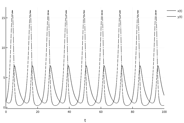
Figure 1: Solution of system (1)

First, load the required packages (if needed):

⬇

import Pkg

Pkg.add("ModelingToolkit")

Pkg.add("OrdinaryDiffEq")

Then, we load the package for plot construction:

⬇

Pkg.add("Plots")

and then link the required packages:

⬇

using ModelingToolkit

using OrdinaryDiffEq

using Plots

Now, we are ready to solve the problem. Declare variables and differentiation operators. A part of the variables is declared as parameters.

⬇

@parameters t a b c d

@variables x(t) y(t)

@derivatives D’~t

Now, we simply rewrite system (1) using the syntax of Julia:

⬇

eqs = [D(x) ~ a *x - b*x*y,

D(y) ~ c*x*y - d*y]

By symbolic manipulations, we reduce the system to the form that is required for the package OrdinaryDiffEq.lj rackauckas:2017:differentialequations.jl :

⬇

sys = ODESystem(eqs)

The further manipulations are performed within the package OrdinaryDiffEq.lj. Set the initial values of the variables:

⬇

u0 = [x => 1.0

y => 1.0]

We also specify the problem parameters:

⬇

p = [a => 1.1

b => 0.4

c => 0.1

d => 0.4]

We will solve the problem on the time interval

⬇

tspan = (0.0,100.0)

Create the structure describing the entire problem:

⬇

prob = ODEProblem(sys,u0,tspan,p; jac=true)

The additional parameter

jac=true} instructs the
system to symbolically generate the optimized Jacobi
function for improving the work of differential equation solvers.
Finally, we apply the solver available in the package
OrdinaryDiffEq.lj:
\begin

mintedjulia sol = solve(prob) Now, we plot the solution (see Fig. 1):

⬇

plot(sol)

This approach fits well into the idea of a specialized language for scientific and engineering computations. Under this approach, symbolic computations are performed not by using a special universal language, but a special problem-oriented symbolic computation language is created for each direction. This language should seamlessly fit with the basic language (Julia in the case under consideration).

V Conclusion

The (incomplete) survey of computer algebra systems that can be used with Julia showed that the language itself and its infrastructure are fairly mature. The computer algebra systems in Julia have a wide of applications—systems for nonprofessional programmers, (SymPy.lj), powerful computer algebra languages (Symata.lj), and domain-specific computer algebra languages (ModelingToolkit.jl). This gives hope that the popularity of Julia will grow not only in the domain of numerical computations but also in the domain of symbolic computations.