Motor-imagery classification model for brain-computer interface: a sparse group filter bank representation model

Abstract

Background: Common spatial pattern (CSP) has been widely used for feature extraction in the case of motor imagery (MI) electroencephalogram (EEG) recordings and in MI classification of brain-computer interface (BCI) applications. BCI usually requires relatively long EEG data for reliable classifier training. More specifically, before using general spatial patterns for feature extraction, a training dictionary from two different classes is used to construct a compound dictionary matrix, and the representation of the test samples in the filter band is estimated as a linear combination of the columns in the dictionary matrix.

New method: To alleviate the problem of sparse small sample (SS) between frequency bands. We propose a novel sparse group filter bank model (SGFB) for motor imagery in BCI system.

Results: We perform a task by representing residuals based on the categories corresponding to the non-zero correlation coefficients. Besides, we also perform joint sparse optimization with constrained filter bands in three different time windows to extract robust CSP features in a multi-task learning framework. To verify the effectiveness of our model, we conduct an experiment on the public EEG dataset of BCI competition to compare it with other competitive methods.

Comparison with existing methods: Decent classification performance for different subbands confirms that our algorithm is a promising candidate for improving MI-based BCI performance.

1 Introduction

Brain-computer interface (BCI) is a new method for the communication and control between the human brain and external devices [1, 2]. Compared with the evoked potential-based BCI, motor imagery (MI) is easily operated and does not rely on external stimuli [3, 4]. It has been suggested to be suitable for the mechanical control and exercise rehabilitation training. MI system shows various applications, such as controlling the movement of a wheelchair, the mouse cursor on the computer screen, and the movement of the left and right direction by imagining the left and right hands [5, 6]. Electroencephalogram (EEG) signal of the brain activities can effectively control the execution of MI tasks. In the past decade, its low cost, non-invasiveness and wide availability have attracted the interest of many researchers [7].

At present, the widely used EEG signals for BCI system control include sensorimotor rhythms (SMRs), event-related potentials (ERP), and visual evoked potentials (VEP) [8, 9, 10, 11, 12]. Particularly, event-related desynchronization / synchronization (ERD / ERS) utilizes the $mu$ rhythm power of sensory motor rhythm (SMR). Recently, a series of BCI has been established based on rhythmic activity recorded on the sensorimotor cortex. SMR draws the attention from BCI using non-invasive neural recording like EEG. SMR is a feature as a band power change within a particular EEG frequency band [3]. At the same time, the EEG band appears in the brain region of sensory organ motion imaging. Therefore, the EEG power conversion can be correlated as the control of MI task.

Until now, many algorithms have been applied to the EEG classification in BCI system [10, 14, 15, 16, 17, 18, 19]. For example, a common spatial pattern (CSP) as a classic feature extraction method was introduced in this field. It uses the spatial features of ERD/ERS, which consists of a spatial filtering technique and simultaneously detects filters maximizing the variance for one class and minimizing the variance for another class [20]. The CSP is greatly effective to classify motor imagery EEG, since the variance of the bandpass filtered signals is equal to the bandpower. This is why CSP plays a key role in discriminating the information of SMR related EEG data [21, 22]. Besides, algorithms combining filter-bank structure with regularization common spatial pattern (RCSP) have also been studied by many researchers. In [10], Park et al. presented RCSP feature extraction on each frequency band, and used mutual information as the individual feature algorithm in a small sample (SS). Moreover, a sub-band regularized common spatial pattern (SBRCSP) used principal component analysis (PCA) to extract RCSP features from all frequency sub-bands [9]. In [10], the author used the filter-bank regularized common spatial pattern (FBRCSP) selected optimum frequency bands for extracting mutual information of RCSP feature. Apart from the methods of feature extraction, another research interest in this field is on the complex classification algorithm to improve the accuracy of EEG classification and provide good robustness [23, 24, 25, 26, 27, 28, 29, 30, 31, 32]. In earlier studies, with the assumption that sample covariance matrix of different classes are similar, linear discriminant analysis (LDA) was used as the main algorithm to distinguish the two types of motor imagination [33, 34]. In order to improve the generalization ability of the model, numerous regularization classifications have been applied for SMR classification. For instance, Mahanta et al. improved the reliability of the classifier by regularized LDA to correct inaccuracy of estimated covariance matrices [35]. Moreover, the sparse representation classification (SRC) which has been successfully applied in the image field [36, 37] is also employed in many studies. The SRC aims to estimate the sparse representation of the test samples as a linear combination of the columns (ie, training samples) in the dictionary matrix. Then, we identify the category by minimizing the reconstruction error, the labels of the test samples are determined by detecting which class the training samples providing the smallest residual norm belong to [43]. Many studies show that by introducing the SRC scheme, the classification accuracy on SMR can be distinctly improved [38, 39, 40, 41, 42].

Many previous researchers focused on SMR feature extraction and pattern recognition. Then, when the dimensions of the training data are insufficient, the number of training samples cannot truly reflect the distribution of features, which can lead to unsatisfactory results. In order to obtain relatively large data, a long calibration time is required during BCI experiment acquisition, which will affect the practicality of the system. On the other hand, some research try to reduce the sample size as much as possible without sacrificing classification accuracy.

In order to address the SMR classification in the SS situation and decrease the calibration time of the BCI system, we propose a novel sparse group filter bank representation model (SGFB). The most compact representation of the test sample is estimated as a linear combination of columns in the dictionary matrix. Moreover, unlike the SRC scheme using only $L_{1}$-norm regularization, the SGFB introduces two penalty factors ($L_{1,2}$-norm) to control the sparsity by frequency bands, which effectively and automatically select frequency bands from a sparse group representation of the test samples and exclude those which provide no contribution. To be specific, the EEG signals in the range of 4-40Hz are divided into subbands with a range of 4Hz, i.e., 4-8Hz, 8-12Hz, 12-16Hz, 16-20Hz,$\cdots$,36-40Hz by a filter bank that consists of a five-order butterworth bandpass filter. Furthermore, CSP is applied to the divided signals by the filter bank. Finally, we apply the SGFB method for the BCIs and the output of classification. The performance of the SGFB algorithm is evaluated by the classification accuracy for five subjects in the BCI competition III dataset IVa. The good results we obtained suggest our method provides a new direction for the classification of the small sample sets for MI. Furthermore, for the filter band optimization, the EEG segmentation time window is an important issue and has a certain interpretation of the correlation among features [44]. In an MI system, subjects is usually required to complete certain tasks. However, the brain’s response time to psychological tasks is an unknown parameter. In the MI tasks, 0-1 s is considered to be the preparatory stage before the mission, while the period between 3.5 and 4 seconds is a later stage.

The remainder of this paper is organized as follows. The previous work is introduced in Section 2.3. In Section 2, mathematical methods which include the CSP feature extraction method, the sparse filter bank, and the filter bank group sparse representation are introduced. In Section 3, a brief description on the experimental procedures is provided. Results and discussion are given in Section 4. This paper ends with a conclusion in Section 5.

2 Problem formulations and the proposal of SGFB model

2.1 Mathematical Symbols

To state the rest of our study more clearly, we first list the mathematical symbols and their meanings in this paper as below. We denote vectors and matrices as ltalian italics. Furthermore, we define the main notations in the tab 1.

Table 1: Definitions of main notations

Parameter	Description	Definition
$\it{X}\in{\mathbb{R}^{m\times n}}$	The EEG signal with K class	$\it{{{X}=[X_{1},X_{2},\cdots,X_{K}]}}$
$\it{{X_{K}}}\in{R^{m*{n_{k}}}}$	The training samples labeled	$\it{{{X_{K}}=[X_{1}^{k},X_{2}^{k},\cdots,X_{nk}^{k}]}}$
	with the $k$th class
$\it{{W}}\in\mathbb{R}^{N\times 2M}$	Spatial filter	$\it{{W=\left[{{w_{1}},\cdots,{w_{2M}}}\right]}}$
$D\in\mathbb{R}^{2M\times(N1+N2)}$	Composite matrix of single	$D=[D_{Left},D_{Right}]$
	frequency band
$\it{\widetilde{D}_{f}}\in{\mathbb{R}^{2M\times F}}$	The composite matrix with 8	$\it{\widetilde{D}_{f}=[D_{f1},D_{f2},\cdots,D_{f9}]}$
	frequency bands
$\it{y}\in{\mathbb{R}^{m\times 1}}$	Test sample	${y}=[y_{1},y_{2},\cdots,y_{n}]$
$\it{{\widetilde{D}}}\in\mathbb{R}^{2M\times i}$	Component dictionary matrix	$\it{{\widetilde{D}=\left[{{D_{l,1}},{D_{l,2}},\cdots,{D_{l,{N_{l}}}}}\right]}}$
$\it{u^{*}}$	Band sparse weight	$\it{{u^{*}}=\left[{u_{1}^{*},u_{2}^{*},\cdots,u_{n}^{*}}\right]}$
$\it{{X_{L}},{X_{R}}}$	Left and right motor-	$\it{{X_{L}},{X_{R}}}\in{\mathbb{R}^{2n\times T}}$
	imagery signal
$\it{X_{L}^{CSP},X_{R}^{CSP}}$	Left and right motor-imagery	$\it{X_{L}^{CSP},X_{R}^{CSP}}\in{\mathbb{R}^{2n\times T}}$
	signal extracted by CSP
$\it{{\delta_{l}}}:{\mathbb{R}^{N}}\to{\mathbb{R}^{N}}$	Characteristic function	-

2.2 Common spatial pattern (CSP)

We assume an EEG epoch with $N_{t}$ time samples from $N_{n}$ channels. This EEG signal first passes through a set of $N_{f}$ bandpass filters. Denote the data set of training samples labeled with the $k$th class as

$${\it{{X_{k}}=[X_{1}^{k},X_{2}^{k},\cdots,X_{nk}^{k}]}}\in{\mathbb{R}^{m\times{n_{k}}}}$$ (1)

where each element is a training sample, $m$ is the dimension of the feature space and $n_{k}$ is the total number of $X_{k}$. It supposes that the dictionary define the samples to be classified as ${\it{{X}=[X_{1},X_{2},\cdots,X_{K}]}}\in{\mathbb{R}^{m*n}}$, $K$ denotes the number of class and $n=\sum\nolimits_{i=1}^{K}{{n_{i}}}$. Given a query sample $\it{y}\in{\mathbb{R}^{m}}$, the task of pattern recognition is to determine which class $y$ belongs to.

Matrix $\it{X_{j}}$ refers to the EEG signal filtered in the $j^{th}$ filter bank for a single trial, the sample covariance matrix $\it{C}$ for $\it{X_{j}}$ is calculated as

$$C=\it{\frac{{{X_{j}}X_{j}^{T}}}{{tr\left({{X_{j}}X_{j}^{T}}\right)}}}$$ (2)

Suppose the EEG data obtained from a temporal interval in the $ith$ trial of class $l$ ($l=-1~{}or~{}+1$) and assume that the EEG samples have removed the mean within a given frequency band, then the spatial covariance matrix of the category $l$ can be calculated as

$$\it{\sum\nolimits_{l}=\frac{1}{{{N_{l}}}}\sum\nolimits_{i=1}^{N{}_{l}}{{X_{i,l}}}X_{i,l}^{T}}$$ (3)

where $N_{l}$ is the number of trials belonging to the class $l$, and $T$ denotes the transpose operator. CSP aims at seeking spatial filters (i.e., linear transforms) to maximize the ratio of transformed data variance between two classes as

$$\it{\mathop{\max}\limits_{w}J\left(w\right)=\frac{{{w^{\rm T}}\sum\nolimits_{1}w}}{{{w^{\rm T}}\sum\nolimits_{2}w}}~{}~{}~{}~{}~{}~{}~{}{\rm{s}}{\rm{.t}}{\rm{.}}~{}~{}~{}~{}{\left\|w\right\|_{2}}}=1$$ (4)

where ${\it{w}\in\mathbb{R}^{C}}$ is a spatial filter and $\|{\cdot}\|$ is the $l_{2}$-norm. The CSP filter matrix $W$ consists of the column vector $\it{{w_{i}}}$. This can be achieved by equivalently solving a generalized eigenvalue problem $\sum\nolimits_{1}{\it{w}}=\lambda\sum\nolimits_{2}{\it{w}}$. By collecting eigenvectors corresponding to the largest and smallest generalized eigenvalues of the $M^{*}$, a set of spatial filters are obtained from $\it{W}$. For a given EEG sample ${\it{X}}$, the feature vector is formed as ${\it{Z}}$ with entries as follow,

$${{\rm Z}_{m}}=\log\left({{\mathop{\rm var}}\left({w_{m}^{T}X}\right)}\right)~{}~{}~{}~{}~{}~{}~{}{\rm{m=1,}}\cdots{\rm{,2M^{*}}}$$ (5)

where var($\cdot$) denotes the variance.

Given two types of EEG training signals, ${\it{X_{L}}}$ and ${\it{X_{R}}}$, we define the CSP filtered signal as

$$\begin{array}[]{l}{\it{X_{R}^{CSP}}}=W_{CSP}^{T}{X_{R}}\\ {\it{X_{L}^{CSP}}}=W_{CSP}^{T}{X_{L}}\end{array}$$ (6)

The EEG samples ${\it{{X_{i,l}}}}$ is the bandpass filtered on different bands instead of just a single frequency band, the CSP features can be extracted on each frequency band. Hence, the dimensionality of the feature vector is expanded to be 2M$\times$ N by concatenating all of the features. Note that, the successful application of CSP highly depends on the selection of filter bands. The optimal filter band is generally subject-specific. An increasing number of studies have suggested that the accuracy of MI classification can be significantly improved by the optimization of the filter band.

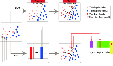
Figure 1: The block diagram of the SVM and sparse representation method.

2.3 Sparse representation classification (SRC)

We have mentioned that $X$ is the training sample. In addition, $\it{X_{ij}}$ and ${n_{i}}$ represent the $j$th training sample and the number of training samples from the $i$th class respectively. Furthermore, the test signal $\it{y}\in\mathbb{R}^{m}$ can be sparsely represented as a linear combination of some columns of $\it{X}$, where ${\vartheta}\in{\mathbb{R}^{n}}$ is a coefficient vector corresponding to $\it{X}$. For a test sample ${\vartheta}\in{\mathbb{R}^{n}}$, its representation under all the training samples is

$$\begin{array}[]{l}y={X_{1}}{\vartheta_{1}}+{X_{2}}{\vartheta_{2}}+\cdots+{X_{c}}{\vartheta_{c}}\\ {\rm{}}={X_{11}}{\vartheta_{11}}+{X_{12}}{\vartheta_{12}}+\cdots+{X_{c{n_{c}}}}{\vartheta_{c{n_{c}}}}\\ {\rm{}}=X\vartheta\end{array}$$ (7)

Therefore, the sparse solution of Eq. 7 can be represented by Eq. 8.

$$\mathop{\arg\min}\limits_{\vartheta}\left\|{\varphi-Z\vartheta}\right\|_{2}^{2}+\lambda f\left({{{\left\|\vartheta\right\|}_{p}}}\right)$$ (8)

where $\varphi$ and $Z$ are the test sample and the training samples, respectively. $f\left({{{\left\|\vartheta\right\|}_{p}}}\right)$ serves as an adjustable penalty function of $l_{p}$-norm constrained, and $\lambda>0$ is a limiting parameter, a larger $\lambda$ can obtain a greater degree of sparse solution. According to the changes in $\it{Z}$, $\it{\varphi}$ and $p$, when Equation 9 is minimized, we get the sparse ground coefficient vector. $\it{{\vartheta^{*}}}$. Let $\it{{\delta_{i}}\left({{\vartheta^{*}}}\right)}$ be a vector whose only nonzero entries are associated with class $i$, the class label of $\it{y}$ can be decided as $\it{y}$ that gives the minimum reconstruction error, i.e.,

$$y=\mathop{\arg\min}\limits_{\vartheta}{\left\|{\varphi-Z{\delta_{i}}\left({{\vartheta^{*}}}\right)}\right\|_{2}}$$ (9)

Besides, we show the commonly used SVM and sparse representation frameworks using the BCI in the Fig. 1.

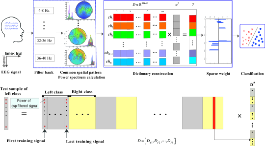
Figure 2: The block diagram of the filter bank group sparse representation method. We define a component dictionary matrix $\widetilde{D}=\left[{{D_{l,1}},{D_{l,2}},\cdots,{D_{l,{N_{l}}}}}\right]$, and the $\widetilde{D}$ is a matirx of size $2M\times N$, $u^{*}$ is of size $N\times 1$ and is divided into $K+1$ non-overlapping group ${u_{0}},{u_{1}},{u_{2}},\cdots,{u_{K}}$.

2.4 Sparse group filter bank (SGFB)

Our proposed method is based on the SGFB framework, i.e., we use the different frequency bands (4-8Hz, 8-12Hz, … , 36-40Hz). The block diagram of the filter bank group sparse representation method is shown in Fig. 2. SRC is used in many applications [48], especially in face recognition. SGFB is an extended approach of the SRC, which can provide the new idea in MI classification tasks. The CSP feature of the test samples are in the form of a linear combination and are superior to the LDA method in the MI classification of BCI. In our algorithm, we design the dictionary matrix to represent the test samples.

Although many algorithms have achieved significant results in MI classification, it is difficult to provide satisfactory results when the size of available train samples is small. Furthermore, to achieve better classification performance, relatively large system calibration time is required for larger EEG data. Therefore, to avoid sacrificing classification accuracy and obtain significant results with small data, we propose a new classification framework based on SGFB.

Suppose that the number of training samples for each class $l$ is $N_{l}$ ($l$ = 1 for the left hand, and the $l=2$ for the right hand). Denote $\widetilde{D}=\left[{{D_{l,1}},{D_{l,2}},\cdots,{D_{l,{N_{l}}}}}\right]$ as the combined dictionary matrix of class $l$, where the column vectors $\it{{D_{l,i}}}\in{\mathbb{R}^{2M\times 1}}$ $(i=1,2,\cdots,N_{l})$ are the CSP features obtained by 4. Then, with the constructed dictionary matrix, we will use SGFB to find the best sparse representation vector $u^{*}$.

The coherence measures the correlation between the two component dictionaries defined in the following way:

$$M\left({{D_{L}},{D_{R}}}\right)\buildrel\Delta\over{=}\max\left\{{\left|{\left\langle{{D_{L,j}},{D_{R,k}}}\right\rangle}\right|:j,k=1,2,\cdots,{N_{l}}}\right\}$$ (10)

The vector ${D_{L,j}}$ is the $j^{th}$ column of ${D_{L}}$; similarly, ${D_{R,k}}$ is the $k^{th}$ column of ${D_{R}}$. The notation $\left\langle{{D_{L,j}},{D_{R,k}}}\right\rangle$ denotes the inner product of two vectors. We call $M$ the measure of mutual coherence of the two component dictionaries; when $M$ is small, we say that the complete dictionary is incoherent.

By this method, we construct a complex dictionary matrix from different frequency bands, which includes not only the training samples collected on the frequency band (8-13Hz) that many researchers have already investigated, but also on the frequency bands that are rarely considered before. As a result, good classification effect can be obtained even for a relatively limited amount of the training samples. Applying sparsity to the entire training set, the SGFB estimates the optimal representation vector, and the $\ell_{1}$ norm regularization is employed to further exclude those insignificant frequency bands. A detailed description of the SGFB method is given below.

We collect EEG training data from 9 different frequency bands. We then use the CSP method for feature extraction and derive K+1 dictionaries $D_{f1},D_{f2},...D_{f9}$ in different frequency bands, which are concatenated later into a conforming matrix $\widetilde{D}$. The compounding different frequency bands to form a composite matrix and our SGFB method is designed to estimate the best representation vector $u^{*}$ as:

$${\it{{u^{*}}}}=\mathop{\arg\min}\limits_{u}\frac{1}{2}\left\|{y-\widetilde{D}{u}}\right\|_{F}^{2}+\lambda{\left\|u\right\|_{1}}$$ (11)

where $\lambda$ denotes the Hyperparameter. In order to generate a sparse vector for the samples of $u^{*}$, the quadratic constraint is

$$\mathop{\arg\min}\limits_{\it{u}}\sum\limits_{i=1}^{n}{\left\|{{\it{{u_{i}}}}-\frac{1}{n}\sum\limits_{j=1}^{n}{{\it{{u_{j}}}}}}\right\|}_{2}^{2}$$ (12)

To make the sparse vector as close as possible to its concentrated vector, we update Eq. 11 as shown in Eq. 13.

$$\mathop{\arg\min}\limits_{u}\frac{1}{2}\left\|{y-\widetilde{D}{u}}\right\|_{F}^{2}+\lambda{\left\|u\right\|_{1}}+\frac{{{\lambda_{1}}}}{2}\sum\limits_{i=1}^{n}{\left\|{{u_{i}}-\frac{1}{n}\sum\limits_{j=1}^{n}{{u_{j}}}}\right\|_{2}^{2}}$$ (13)

The hyperparameter $\lambda_{1}$ is the constraint parameter, which improves the generalization ability of the model by controlling the sparsity of $u^{*}$ and the sparsity between groups of these subbands. The optimal sparse matrix ${u^{*}}$ can generate not only similar sparse decompositions, but also similar weights. Therefore, if $u_{ik}^{*}$ and $u_{jk}^{*}$ are not zero, they should be with the same sign, namely, $u_{ik}^{*}\times u_{jk}^{*}>0$.

Given data $y$, $\widetilde{D}_{f}$, and the parameters $\lambda$ and $\lambda_{1}$, if $u_{ik}^{*}\times u_{jk}^{*}>0$, then $u_{ik}^{*}$ and $u_{jk}^{*}$ have ${\mathop{\rm sgn}}\left({u_{ik}^{*}}\right)={\mathop{\rm sgn}}\left({u_{jk}^{*}}\right)$, where ${\mathop{\rm sgn}}\left(\bullet\right)$ denotes the sign function, Eq. 11 is transformed into

$$L\left({{c_{i}},\lambda,{\lambda_{1}}}\right)=\frac{{\rm{1}}}{{\rm{2}}}\left\|{y-\widetilde{D}u}\right\|_{F}^{2}+\lambda{\left\|{{u_{i}}}\right\|_{1}}+\frac{{{\lambda_{1}}}}{{\rm{2}}}\sum\limits_{i=1}^{n}{\left\|{{u_{i}}-\frac{1}{n}\sum\limits_{j=1}^{n}{{u_{j}}}}\right\|}_{2}^{2}$$ (14)

in this case, $u_{i}^{*}$ should satisfy $(if\left({\it{{u_{{i_{k}}}}}^{*}\neq 0}\right))$

$$\frac{{\partial L\left({{u_{i}},\lambda,{\lambda_{1}}}\right)}}{{\partial{u_{ik}}}}\left|\begin{array}[]{l}\\ {u_{i}}=u_{i}^{*}\end{array}\right.=0$$ (15)

It obtains

$$\begin{array}[]{l}-\alpha_{k}^{T}\left({{y_{i}}-\widetilde{D}u_{i}^{*}}\right)+\lambda{\mathop{\rm sgn}}\left({u_{ik}^{*}}\right)+\\ {\lambda_{1}}\left({1-\frac{1}{n}}\right)\left({u_{ik}^{*}-\frac{1}{n}\sum\nolimits_{t=1}^{n}{u_{tk}^{*}}}\right)=0\end{array}$$ (16)

$$\begin{array}[]{l}-\alpha_{k}^{T}\left({{y_{j}}-\widetilde{D}u_{j}^{*}}\right)+\lambda{\mathop{\rm sgn}}\left({u_{jk}^{*}}\right)+\\ {\lambda_{1}}\left({1-\frac{1}{n}}\right)\left({u_{jk}^{*}-\frac{1}{n}\sum\nolimits_{t=1}^{n}{u_{tk}^{*}}}\right)=0\end{array}$$ (17)

Subtract equation 16 and 17 as follow,

$$\alpha_{k}^{T}\left({{r_{j}}-{r_{i}}}\right)+{\lambda_{1}}\left({1-\frac{1}{n}}\right)\left({u_{ik}^{*}-u_{jk}^{*}}\right)=0$$ (18)

which gives an equivalent form as

$$u_{ik}^{*}-u_{jk}^{*}=\frac{n}{{\left({n-1}\right){\lambda_{1}}}}\alpha_{k}^{T}\left({{r_{i}}-{r_{j}}}\right)$$ (19)

where ${y_{i}}-\widetilde{D}u_{i}^{*}$ is the residual vector. We can update the Eq. 19 and implies that

$$\begin{array}[]{l}\left|{u_{{i_{k}}}^{*}-u_{{j_{k}}}^{*}}\right|=\frac{n}{{\left({n-1}\right){\lambda_{1}}}}\left|{\alpha_{k}^{T}\left({{r_{i}}-{r_{j}}}\right)}\right|\\ ~{}~{}~{}~{}~{}~{}~{}~{}~{}~{}~{}~{}~{}~{}\leq\frac{n}{{\left({n-1}\right){\lambda_{1}}}}{\left\|{{\alpha_{k}}}\right\|_{2}}{\left\|{{r_{i}}-{r_{j}}}\right\|_{2}}\\ ~{}~{}~{}~{}~{}~{}~{}~{}~{}~{}~{}~{}~{}~{}\leq\frac{1}{{\left({n-1}\right){\lambda_{1}}}}{\left\|{{r_{i}}-{r_{j}}}\right\|_{2}}\end{array}$$ (20)

For calculating the optimal solution, we have rewritten Eq. 12 as Eq. 21

$$\begin{array}[]{l}{\rm{}}\sum\limits_{i=1}^{n}{\left\|{{u_{i}}-\frac{1}{n}\sum\limits_{j=1}^{n}{{u_{j}}}}\right\|_{2}^{2}}\\ =\left\|{u-u\frac{1}{n}{{11}^{\text{T}}}}\right\|_{F}^{2}\\ =\left\|{u\left({I-\frac{1}{n}{{11}^{T}}}\right)}\right\|_{F}^{2}\\ =Tr\left({u{{\left({I-\frac{1}{n}{{11}^{T}}}\right)}^{2}}{u^{T}}}\right)\\ =Tr\left({uM{u^{T}}}\right)\end{array}$$ (21)

where $Tr\left(\cdot\right)$ denotes the trace and ${\left(\cdot\right)^{T}}$ denotes the transpose of a matrix, the $M={\left({I-\frac{1}{T}{{11}^{T}}}\right)^{2}}\in{\mathbb{R}^{T\times T}}$ $(I\in\mathbb{R}^{T\times T}\text{is the unit matrix and}~{}1=[1,\cdots,1]^{T}\in\mathbb{R}^{T})$. Hence, we can update the Eq. 13 as

$$\mathop{\arg\min}\limits_{i}\frac{1}{2}\left\|{y-\widetilde{D}{u^{*}}}\right\|_{F}^{2}+\lambda{\left\|u\right\|_{1}}+\frac{{{\lambda_{1}}}}{2}Tr\left({uM{u^{T}}}\right)$$ (22)

The $c_{i}$ is updated by fixing the vector ${\left\{{{u_{j}}}\right\}_{j\neq i}}$, and the optimization process is as

$$\mathop{\arg\min}\limits_{i}\frac{1}{2}\left\|{y-\widetilde{D}{u_{i}}^{*}}\right\|_{2}^{2}+\frac{{{\lambda_{1}}}}{2}{M_{ii}}u_{i}^{T}{u_{i}}+u_{i}^{T}{h_{i}}+\lambda{\left\|{{u_{i}}}\right\|_{1}}$$ (23)

where ${h_{i}}={\lambda_{1}}\left({\sum\limits_{j\neq i}{{M_{ij}}{c_{j}}}}\right)$. Here, we need to look for the signs of the coefficients $c_{i}^{j}$ of $c_{i}$. Once all the signs of $c_{i}^{j}$ are determined, the Eq. 23 can be transformed into an unconstrained optimization problem. In this paper, we define $h\left({{u_{i}}}\right)=\frac{1}{2}\left\|{y-\widetilde{D}{u_{i}}}\right\|_{2}^{2}+\frac{{{\lambda_{1}}}}{2}{M_{ii}}u_{i}^{T}{u_{i}}+u_{i}^{T}{h_{i}}$ and $\nabla_{i}^{h}\left|{h\left({{u_{i}}}\right)}\right|=\frac{{\partial h\left({{u_{i}}}\right)}}{{\partial u_{i}^{j}}}$

If $\widetilde{D}$ is large, the values in the calculated system vector will be small. In order to solve this problem, we normalize each column of $\widetilde{D}$ so that the $\ell 2$ norm value of each column is less than or equal to 1. The normalized matrix set $\widetilde{D}$ is obtained by the Eq. 24.

$$\widetilde{D}=\left\{{\widetilde{D}\in{R^{m\times k}}~{}~{}s.t.~{}\forall j=1,\cdots,k,d_{j}^{T}{d_{j}}\leq 1}\right\}$$ (24)

In principle, we calculate the minimum reconstruction error to determine the classification label that the test sample belongs to. Specifically, ${\delta_{l}}:{\mathbb{R}^{N}}\to{\mathbb{R}^{N}}$ as a characteristic function to select the coefficient related to class $l$. $u^{*}$ with all non-zero coefficients are associated with the columns of a single category $l$ in the dictionary matrix $\widetilde{D}$. Then, the calculation of the sparse coefficient vector is realized by the Lars algorithm[49].

$$\begin{array}[]{l}{r_{i}}\left({\overline{y}}\right)={\left\|{\overline{y}-{{\overline{y}}_{l}}}\right\|_{2}}\\ ~{}~{}~{}~{}~{}~{}~{}{\rm{=}}~{}{\left\|{\overline{y}-\widetilde{D}{\delta_{l}}\left({{u^{*}}}\right)}\right\|_{2}}\end{array}$$ (25)

we approximate the test sample as ${{\it{{{\overline{y}}_{l}}}}}={\widetilde{D}{\delta_{l}}\left({{u^{*}}}\right)}$ and calculate the residuals between ${\overline{y}}$ and ${{{\overline{y}}_{l}}}$ to determine the category which the minimum reconstruction error belongs to.

$${\rm{class}}\left(\bar{y}\right)=\mathop{\arg\min}\limits_{i}{r_{i}}\left({\it{\bar{y}}}\right)$$ (26)

The column vectors in $D$ corresponding to those zero entries in $u^{*}$ are excluded to form a optimized feature set $\tilde{D}$ that is of lower dimensionality. The given $\lambda$ and $\lambda_{1}$ determine the sparsity degree of $u^{*}$, correspondingly the selection of CSP features.

For the new test sample, the corresponding subband feature vector ${D_{l,{N_{l}}}}\in{R^{2M\times N}}$ is estimated by CSP. According to the sparse vector $u^{*}$, the optimal feature is selected, and then MI classification is determined by the minimum redundancy error.

Besides, we summarize the process of the algorithm of the SGFB optimization and the classification process in Algorithm $1$ and Algorithm $3$ respectively.

3 Experimental datasets and evaluation

3.1 EEG data description

In this paper, we use the BCI competition III dataset IVa that is publicly available to evaluate the performance of the proposed algorithm. More details can be found at http://www.bbci.de/competition. These datasets are effective to evaluate the performance of the algorithms, which has been used in many studies.

The BCI competition III dataset IVa is available in 1,000Hz version and 100Hz version. In this experiment, we use the 100Hz version and 1-2s interval of 3.5s motor imagery EEG. The EEG signal is obtained from five healthy subjects (aa, al, av, aw and ay). The subjects sit in a comfortable chair and perform motor imagery experiments. The EEG signal is recorded by using 118 channels and 140 trials for each class. The classes consist of the right hand and foot, i.e., the EEG signal is provided with a total of 280 trials for each subject.

Instead of performing band-pass filtering on the original EEG segment, we perform a set of sub-band filtering, selecting 9 sub-bands from the frequency range of 4-40Hz, and the bandpass is 4Hz, i.e., 4-8Hz, 6-10Hz, … , 36-40Hz. Subsequently, the CSP features can be extracted from the EEG segments of each subband.

3.2 Experimental evaluation

Our experiment consists of five steps. Firstly, the EEG signal is divided by the frequency range of 4-40Hz into 9 bands. This filter bank consists of a bandpass filter. The range of each band is 4-8Hz, 8-12Hz, $\cdots$, 36-40Hz respectively. Shin et al. explored the effectiveness of different CSP numbers for MI classification tasks [42]. Secondly, we apply CSP to the signal derived from the filter bank and the 32 spatial filters. As a next, the band power is calculated in different filter banks. Thirdly, the dictionary learning with $\ell 1$ minimization is employed in different filter bank. Finally, the label for each data is assigned by using the ensemble.

The Classification performance is evaluated based on classification accuracy (ACC), sensitivity (SEN), and specificity (SPE). These statistical measures are defined as follow:

$$ACC=\frac{TP+TN}{TP+FP+TN+FN}$$ (27)

$$SEN=\frac{TP}{TP+FN}$$ (28)

$$SPE=\frac{TN}{TN+FP}$$ (29)

where TP, TN, FP and FN denote the true positive, true negative, false positive and false negative, respectively. Thus, ACC measures the proportion of subjects correctly classified among all subject, SEN and SPE correspond to the proportions of left hand and right hand classified, respectively.

4 Results and discussion

In the past few years, researchers have developed a series of algorithms in MI. In this paper, We proposed a complex model of SGFB to improve MI classification accuracy. The relevant results are described in Table 3. Besides, we performed a statistical comparison of the performance of (C3-C4), CSP, FBCSP, and SGFB. Moreover, we used the 10-fold cross-validation. We marked the average accuracy in the SGFB method in bold for each sample. Besides, We will discuss the impact of different parameters on classification accuracy in Section 4.1.

Table 2: Procedures required by each of the compared methods.

Method	Procedures
(C3-C4)+SVM	Bandpass filtering + Variance calculation + SVM
CSP+SVM	Bandpass filtering + CSP + SVM with parameter selection
FBCSP+SVM	Multi-subband filtering + CSP + SVM with parameter selection
FBCSP+SRC	Multi-subband filtering + SRC
SGFB	Multi-subband filtering + CSP + Sparse learning with parameter selection

To comprehensively investigate the effectiveness of our proposed method on training data reduction, we further tested the classification accuracy by using different numbers of training samples from the target subject. In particular, we randomly select 30%, 50%, 70% and 100% samples (TS) from each target subject and evaluate the classification accuracy based on repeating the above steps 10 times. The tab. 4, 5, 6 and 7 describe the average MI classification accuracy obtained by SGFB for 30%, 50% 70%, and 100% samples, respectively. The results show that even if only 30% of the samples can be used for training to obtain 81.16% accuracy, this confirms the potential prospect of our model in MI classification with only a few training samples.

\psfrag{t}[c][c][0.7]{$t$ (s)}\psfrag{hc1}[c][c][0.6]{~{}~{}$\hat{c}_{1}$}\psfrag{hc2}[c][c][0.6]{$\hat{c}_{2}$}\includegraphics[scale={0.13}]{fig2-1a.eps}

\psfrag{t}[c][c][0.7]{$t$ (s)}\psfrag{hc1}[c][c][0.6]{~{}~{}$\hat{c}_{1}$}\psfrag{hc2}[c][c][0.6]{$\hat{c}_{2}$}\includegraphics[scale={0.13}]{fig2-1b.eps}

\psfrag{t}[c][c][0.7]{$t$ (s)}\psfrag{hc1}[c][c][0.6]{~{}~{}$\hat{c}_{1}$}\psfrag{hc2}[c][c][0.6]{$\hat{c}_{2}$}\includegraphics[scale={0.54}]{fig6.eps}

Figure 3: Performance of different classification tasks. (a) Discriminant vectors $u^{*}$ and feature distributions of subject ay, derived by SGFB. The vertical axis of the upper and lower subgraphs represents the weight of the discrimination vector. Large weights indicate that the corresponding features are more important for MI classification. (b)The scatter plot of two category features. (c) Comparison of the recognition accuracy for different TS situations.

Table 3: Recognition accuracy (%) obtained by (C3-C4)+SVM, CSP+SVM (8-12Hz), CSP+SVM (4-40), FBCSP+SVM (multi-subband) and SGFB (multi-subband), respectively, at different time window (TW), for the BCI Competition IV dataset IVb.

TW	Method	Subject					Average
		aa	al	av	aw	ay
1-2 (1s)	(C3-C4)+SVM (8-12 Hz)	54.62	57.36	57.82	59.31	54.47	56.71
	CSP+SVM (8-12 Hz)	75.52	79.1	73.67	76.33	71.05	75.13
	CSP+SVM (4-40 Hz)	79.9	84.4	89.2	80.61	80.7	84.96
	FBCSP+SVM (multi-subband)	55.91	79.58	63.25	73.53	78.56	70.17
	SGFB (multi-subband)	83.57	95.36	88.21	81.07	93.21	88.28
2-3 (1s)	(C3-C4)+SVM (8-12 Hz)	57.65	73.5	68.66	70.1	72.67	68.52
	CSP+SVM (8-12 Hz)	66.9	87.65	71.85	82.5	82	77.98
	CSP+SVM (4-40 Hz)	77.7	78.2	74.44	77.12	78.57	77.2
	FBCSP+SVM (multi-subband)	55.85	61.19	60.05	65.24	71.46	62.78
	SGFB (multi-subband)	74.64	91.07	77.86	84.64	92.86	84.21

Table 4: Classification results achieved by the SGFB for left and right EEG signals (30% TS).

	evluation	Subject					Average
		aa	av	aw	ay	al
	Acc	73.57	81.43	84.02	78.21	88.57	81.16
	Spec	82.86	94.29	77.86	97.86	85	87.58
	Sen	64.29	68.57	90.71	58.57	92.14	74.86

Table 5: Classification results achieved by the SGFB for left and right EEG signals (50% TS).

	evluation	Subject					Average
		aa	av	aw	ay	al
	Acc	75.36	79.29	71.43	79.29	89.29	79.83
	Spec	86.59	97.86	73.57	94.29	85.71	87.6
	Sen	70	60.71	69.29	64.29	92.86	71.43

Table 6: Classification results achieved by the SGFB for left and right EEG signals (70% TS).

	evluation	Subject					Average
		aa	av	aw	ay	al
	Acc	79.64	80	77.14	87.86	95.36	84
	Spec	69.14	90	57.86	99.29	97.86	82.83
	Sen	92.14	65	96.43	76.43	92.86	84.57

Table 7: Classification results achieved by the SGFB for left and right EEG signals (Full TS).

	evluation	Subject					Average
		aa	av	aw	ay	al
	Acc	83.57	88.21	81.07	93.21	95.36	88.28
	Spec	80.07	82.66	98.57	92.14	91.43	88.97
	Sen	86.43	83.57	63.57	94.29	99.29	85.43

\psfrag{t}[c][c][0.7]{$t$ (s)}\psfrag{hc1}[c][c][0.65]{~{}~{}$\hat{c}_{1}$}\psfrag{hc2}[c][c][0.65]{$\hat{c}_{2}$}\includegraphics[scale={0.545}]{fig4.eps}

\psfrag{t}[c][c][0.7]{$t$ (s)}\psfrag{hc1}[c][c][0.65]{~{}~{}$\hat{c}_{1}$}\psfrag{hc2}[c][c][0.65]{$\hat{c}_{2}$}\includegraphics[scale={0.545}]{fig5.eps}

Figure 4: (a). Classification accuracy with different values of parameters $\lambda$ and $\lambda_{1}$ respectively. The results indicate that the performance of our method slightly fluctuates when the values of hyperparameters vary in a relatively large range. In most cases, the classification accuracies are generally stable with respect to the changes of the two hyperparameters, indicating the robustness of our proposed SGFB algorithm to the parameter values. (b). Average computational time of different methods including SGFB, FBCSP+SVM (multi-subband), (C3-C4)+SVM, CSP+SVM (8-13Hz) and (C3-C4)+SVM respectively.

4.1 Parameter sensitivity

In order to evaluate the effectiveness of the proposed EEG classification method and superior to the existing methods, five other different algorithms are compared to the proposed algorithm using the same dataset.

The 10 Fold cross validation (10FCV) scheme is adopted for evaluation of algorithm performance. In each fold of 10FCV procedure, an additional inner 10FCV is also carried out on the training data to determine the optimal hyperparameters (i.e., $\lambda$ for SFBG and the soft-margin parameter C for SVM). The selection ranges of $\lambda$ and $\lambda_{1}$ are $[0.1,0.2,\cdots,0.9]$ and $\text{[}0.1,\cdots,0.4]$ respectively, while C is selected from $[0.05,0.1,\cdots,1]$. The effectiveness of our proposed method is affected by the selection of hyperparameters, i.e., $\lambda$ for weighted group sparsity and $\lambda_{1}$ for the pattern similarity. In our experiment, we implement a grid search to select the optimal parameter values on the training data using inner 10FCV. To investigate the parameter sensitivity of our proposed algorithm, we evaluate effects of varying values of these two hyperparameters on classification accuracy using 10FCV with all subjects. The best accuracy of 94.64% is achieved by using $\lambda$ = 0.3 for strength weighted sparsity and $\lambda_{1}=0.1$ for similarity constraint. Our future study will further validate performance of the proposed algorithm on a completely independent dataset.

4.2 Computational efficiency

We also compare the computational efficiency of above-mentioned algorithms. Fig. 4-b shows the calculation time evaluated in a MATLAB R2019a environment on a desktop computer with a 3.8 Ghz CPU (i7-7700k, 16G RAM). It suggests that these algorithms can be run on internal loop cross-validation, which is needed for training models. We note that the FBCSP spent the longest calculation time on MI classification. The proposed SGFB algorithm shows comparable computational efficiency with the best accuracy and comparable computational efficiency. At present, in order to explore more complex relationships in the feature space, many subspace regularization algorithms have appeared for various applications including imaging processing and encephalopathy diagnosis [50, 51, 52, 53, 54, 55, 56, 57]. A popular subspace learning method provides an effective method for characterizing feature distributions and has recently been used to improve the correlation of a single event latent classification [58, 59]. This kind of relationship constraint based on manifold learning can further improve the accuracy of classification, which is worthy of our future research [60, 61, 62].

5 Conclusion

In this paper, we introduce a novel SGFB algorithm to construct an efficient classification model in motor imagery-based BCI applications. We construct a compound matrix dictionary for the frequency bands of different rhythms. By combining $L_{2}$-norm and $L_{1}$-norm, a sparse group representation model is designed to control the sparseness between frequency bands to automatically determine the best model. With the public motor imagery-related EEG datasets, extensive experimental comparisons are carried out between the proposed algorithm and two other state-of-the-art methods. The results illustrate the effectiveness of our method in motor imagery BCI applications.

6 Conflict of interest

We declare that we do not have any commercial or associative interest that represents a conflict of interest in connection with the work submitted.

7 CRediT author statement

Cancheng Li: Conceptualization, Methodology, Software, Formal analysis, Investigation, Writing, Original Draft, Visualization. Chuanbo Qin: Investigation, Visualization, Writing Review. Cancheng Li: Formal analysis, Investigation, Visualization, Writing Review. Jing Fang: Writing Review, Resources, Data Curation, Supervision.

8 Acknowledgments

The authors would like to thank the editors and anonymous reviewers for their valuable suggestions and constructive comments, which have really helped the authors improve very much the presentation and quality of this paper. The author would like to acknowledge and thank the organizers of the BCI Competitions III.

9 appendix

Algorithm 1 Pseudo-code Implementation of the Sparse Group Filter Bank Representation (SGFB) Model for Motor Imagery EEG Classification.

0:     $\mathbf{\tilde{D}=\left[{{\tilde{D}_{f1}},{\tilde{D}_{f2}},\cdots,{\tilde{D}_{f9}}}\right]}$, hyperparameter $\lambda$ and $\lambda_{1}$.

0:     The optimal sparse matrix ${u^{*}}={u^{(L+1)}}=\left[{u_{1}^{(L+1)},u_{2}^{(L+1)},\cdots,u_{n}^{(L+1)}}\right]$

1:  Initialize the sparse coefficients and its corresponding sign set;

2:  for $i\leftarrow 1,\cdots,L$  do

3:     for $i\leftarrow 1,\cdots,T$  do

4:        if $the~{}coefficient~{}c_{i}^{(n)}=0$ then

5:           choose $j=\mathop{\arg\max}\limits_{i}\left|{\frac{{\partial{{\left\|{y-\widetilde{D}{u^{*}}}\right\|}^{2}}}}{{\partial u_{j}^{*}}}}\right|$;

6:           if $\frac{{\partial{{\left\|{y-\widetilde{D}{u^{*}}}\right\|}^{2}}}}{{\partial u_{j}^{*}}}>\lambda$ then

7:              set $c_{i}^{j(n)}=-1$;

8:           else if $\frac{{\partial{{\left\|{y-\widetilde{D}{u^{*}}}\right\|}^{2}}}}{{\partial u_{j}^{*}}}<\lambda$ then

9:              set $c_{i}^{j(n)}=1$;

10:           end if

11:        end if

12:     end for

13:     Set feature sign search step according to Algorithm 2

14:  end for

15:  return  coefficient $s$.

Algorithm 2 Set feature sign search step.

1:  (a)  $\widehat{{u^{*}}}$ is a sub-column vector corresponding to the active set in the      complete atomic dictionary ${u^{*}}$

2:  (b)  Calculate the solution of Eq. 11       $\mathop{\arg\min}\limits_{{{\widehat{u}}_{i}}}\left\|{y-\widetilde{D}{u^{*}}}\right\|+\lambda\widehat{\theta}{\widehat{u}_{i}}$;       $\widehat{u}_{i}^{\left(n\right)}={\left({{{\widehat{u}}^{{*^{T}}}}T{{\widehat{u}}^{*}}}\right)^{-1}}\left({{{\widehat{u}}^{{*^{T}}}}y-\frac{{\lambda\widehat{\theta}}}{2}}\right)$;

3:  (c)  Perform a discrete linear search on the close line segment      from $\widehat{u}$ to ${\widehat{u}_{new}}$

4:         (1) Check the target function value of ${\widehat{u}_{new}}$ and the point in             which all coefficient;

5:         (2) Update the value of $\widehat{u}$ to the point with the smallest              objective function value.

6:  (d)  remove the coefficient of zero and update $\theta={\mathop{\rm sgn}}\left({\widehat{u}_{i}^{*\left(n\right)}}\right)$      in the active set;

7:  if $\forall~{}u_{j}^{*}\neq 0$ (for non-zero coefficients) then

8:     $\frac{{\partial{{\left\|{y-\widetilde{D}{u^{*}}}\right\|}^{2}}}}{{\partial u_{j}^{*}}}+\lambda sign\left({u_{j}^{*}}\right)=0$;

9:  end if

10:  if $\forall~{}u_{j}^{*}=0$ (for zero coefficients ) then

11:     $\left|{\frac{{\partial\left\|{y-\widetilde{D}{u^{*}}}\right\|}}{{\partial u_{j}^{*}}}}\right|<\lambda$;

12:  else

13:     continue feature-sign search, go to step (b);

14:  end if

Algorithm 3 SGFB for the EEG Classification.

0:     coefficient s and the test sample signal $\mathbf{y}\in{\mathbb{R}^{m\times 1}}$.

0:     $class(\overline{y})=\mathop{\arg\min}\limits_{i}{r_{i}}\left({\overline{y}}\right)$.

1:  Normalize $\tilde{D}$ and $\overline{y}$ according to Eq.(24)

2:  The optimal representation vector $\mathbf{u^{*}}$ according to Algorithm 1

3:  Compute ${\rm{class}}\left(\bar{y}\right)=\mathop{\arg\min}\limits_{i}{r_{i}}\left(\bar{y}\right)$ 

References

References

- [1] U. Chaudhary, N. Birbaumer, Ramos-Murguialday. A, Brain-computer interface for communication and rehabilitaion. Nat. Rev. Neurosci. 12 (9) (2016) 513–525.
- [2] K. Ang, C. Guan, Brain-computer interface for neurorehabilitaion of upper limb after stroke. Proc. IEEE 103 (6) (2015) 944–953.
- [3] C. Guger, C. Ramoser, G. Pfurtscheller, Real-time EEG analysis with subject-specific spatial patterns for a brain-computer interface (BCI). IEEE Trans. Neural Syst. Rehabil. Eng. 8 (4) (2000) 447–456.
- [4] Y. Yang, S. Chevallier, J. Wiart, I. Bloch, Subject-specific time frequency selection for multi-class motor imagery-based BCIs using few Laplacian EEG channels. Biomed. Signal Process Control 38 (2017) 302–311.
- [5] S. Bozinovski, M. Sestakov, L. Bozinovska, Using EEG alpha rhythm to control a mobile robot. In proc. Annu. Int. Conf. IEEE Eng. Med. Biol. Soc. 3 (1988) 1515–1516.
- [6] B. Blankertz, R. Tomioka, S. Lemm, M. Kawanabe, K. R. Muller, Optimizing spatial filters for robust EEG single-trial analysis. IEEE Signal Proc. Mag. 25 (1) (2008) 41–56.
- [7] C. Vidaurre, B. Blankertz, Towards a cure for BCI illiteracy. Brain Topogr. 23 (2) (2010) 194–198.
- [8] Zhang Y, Wang Y, Zhou GX, Jin J, Wang B, Wang XY, Multi-kernel extreme learning machine for EEG classification in brain-computer interfaces. Expert. Syst. Appl. 96 (2018) 302–310.
- [9] K. K. Ang, Z. Y. Chin, C. Wang, C. Guan, H. Zhang, Filter bank common spatial pattern algorithm on BCI competition IV Datasets 2a and 2b. Frontiers. Neurosci. 6 (2012).
- [10] S.H. Park, D. Lee, S. G. Lee, Filter bank regularized common spatial pattern ensemble for small sample motor imagery classification. IEEE on Neural. Syst. Rehabil. Eng. 2 (2) (2017) 498–505.
- [11] K. K. Ang, Z. Y. Chin, H. Zhang, C. Guan, Mutual informationbased selection of optimal spatial temporal patterns for single-trial EEG based BCIs. Pattern Recognit. 45 (6) (2012) 2137–2144.
- [12] Z. Gu, Z. Yu, Z. Shen, Y. Li, An online semi-supervised brain-computer interface. IEEE Trans. Biomed. Eng. 60 (9) (2013) 2614–2623.
- [13] F. Lotte, M. Congedo, A. Lecuyer, F. Lamarche, B. Arnaldi, A review of classification algorithms for EEG-based brain-computer interfaces. J. Neural Eng. 4 (2) (2007) R1–R13.
- [14] H. Higashi, T. Tanaka, Simultaneous design of FIR filter banks and spatial patterns for EEG signal classification. IEEE Trans. Biomed. Eng. 60 (4) (2012) 1100–1110.
- [15] F. Lotte, F. Guan, Regularizing common spatial patterns to improve BCI designs: Unified theory and new algorithms. IEEE Trans. Biomed. Eng. 58 (2) (2010) 355–362.
- [16] M. Arvaneh, C. Guan, K. K. Ang, C. Quek, Optimizing the channel selection and classification accuracy in EEG-based BCI. IEEE Trans. Biomed. Eng. 58 (6) (2011) 1865–1873.
- [17] S. Siuly, Y. Li, Improving the separability of motor imagery EEG signals using a cross correlation-based least square support vector machine for brain-computer interface. IEEE Trans. Neural. Syst. Rehabil. Eng. 20(4) (2012) 526–538.
- [18] R. Fu, M. Han, Y. Tian, P. Shi, Improvement motor imagery EEG classification based on sparse common spatial pattern and regularized discriminant analysis. J. Neurosci. Meth. 343 (2020) 108833.
- [19] C. Zuo, Y. Miao, X. Wang, L. Wu, J. Jin, Temporal frequency joint sparse optimization and fuzzy fusion for motor imagery-based brain-computer interfaces. J. Neurosci. Meth. 340 (2020) 340, 108725.
- [20] Y. Li, Y. Koike, A real-time BCI with a small number of channels based on CSP. Neural. Comput. Appl. 20 (8) (2011) 1187–1192.
- [21] K. P. Thomas , C. Guan, C. T, Lau, A. P. Vinod, K. K. Ang, A new discriminative common spatial pattern method for motor imagery brain-computer interfaces. IEEE Trans. Biomed. Eng. 56 (11) (2009) 2730–2733.
- [22] W. Wu, Z. Chen, X. Gao, Y. Li, E. N. Brown, S. Gao, Probabilistic common spatial patterns for multichannel EEG analysis. IEEE Trans. Pattern Anal. Machine Intell. 37 (3) (2014) 639–653.
- [23] S. Chen, Z. Luo, H. Gan, An entropy fusion method for feature extraction of EEG. Neural Comput. Appl. 29 (10) (2018) 857–863.
- [24] C. Y. Kee, S. G. Ponnambalam, C. K. Loo, Binary and multi-class motor imagery using Renyi entropy for feature extraction. Neural Comput. Appl. 28 (8) (2017) 2051–2062.
- [25] H. Peng, C. Lei, S. Zheng, C. Zhao, C. Wu, J. Sun, B. Hu, Automatic epileptic seizure detection via Stein kernel-based sparse representation. Comput. Biol. Med. 132 (2021) 104338.
- [26] J. Fang, T. Wang, C. Li, X. Hu, E. Ngai, B. C. Seet, J. Cheng, Y. Guo, X. Jiang, Depression prevalence in postgraduate students and its association with gait abnormality. IEEE Access 7 (2019) 174425–174437.
- [27] T. Wang, C. C. Li, C. Y. Wu, C. J. Zhao, J. Q. Sun, H. Peng, X. P. Hu, B. Hu, A Gait Assessment Framework for Depression Detection Using Kinect Sensors. IEEE Sens. J. 21 (3) (2020) 3260–3270.
- [28] S. Kumar, K. Mamun, A. Sharma, CSP-TSM: Optimizing the performance of Riemannian tangent space mapping using common spatial pattern for MI-BCI. Computer Biol. Med. 91 (2017) 231–242.
- [29] M. Arvaneh, C. Guan, K. K, Ang, C. Quek, Mutual information-based optimization of sparse spatio-spectral filters in brain-computer interface. Neural Comput. Appl. 25 (3-4) (2014) 625–634.
- [30] L. He, b. Liu, D. Hu, Y. Wen, M. Wan, J. Long, Motor imagery EEG signals analysis based on Bayesian network with Gaussian distribution. Neurocomputing 188 (2016) 217-224.
- [31] A. Meziani, K. Djouani, T. Medkour, A. Chibani, A Lasso quantile periodogram based feature extraction for EEG-based motor imagery. J. Neurosci. Meth. 328 (2019) 108434.
- [32] M. Miao, H. Zeng, A. Wang, C. Zhao, F. Liu, Discriminative spatial-frequency-temporal feature extraction and classification of motor imagery EEG: An sparse regression and weighted naive bayesian classifier-based approach. J. Neurosci. Meth. 278 (2017) 13–24.
- [33] P. Xu, P. Yang, X. Lei, D. Yao, An enhanced probalistic LDA for multi-class brain computer interface. PLoS One 6 (2011) e14634.
- [34] C. Vidaurre, M. Kawanabe, P. von Bunau, B. Blankertz, K. R. Muller, Toward unsupervised adaptation of LDA for brain-computer interfaces. IEEE Trans. Biomed. Eng. 58 (3) (2010) 587–597.
- [35] M. S. Mahanta, A. S. Aghaei, K. N. Plataniotis, Regularized LDA based on separable scatter matrices for classification of spatio-spectral EEG patterns. in Proc. IEEE Int. Conf. Acoustics, Speech Signal Process. (2013) 1237–1241.
- [36] J. Wright, A.Y. Yang, A. Ganesh, S. S. Sastry, Y. Ma, Robust face recognition via sparse representation. IEEE Trans. Pattern Anal. Mach. Intell. 31 (2) (2008) 210–227.
- [37] Y. Li, Z. L. Yu, N. Bi, Y. Xu, Z. Gu, Si. Amari, Sparse representation for brain signal processing: a tutorial on methods and applications. IEEE Signal Process. Mag. 31 (3) (2014) 96–106.
- [38] Y. Li, J. Long, L. He, H. Lu, Z. Gu, P. Sun, A sparse representationbased algorithm for pattern localization in brain imaging data analysis. PloS one 7 (12) (2012) e50332.
- [39] Y. Zhang, G. Zhou, J. Jin, Y. Zhang, X. Wang, A. Cichocki, Sparse Bayesian multiway canonical correlation analysis for EEG pattern recognition. Neurocomputing 225 (2017) 103–110.
- [40] Y. Zhang, G. Zhou, J. Jin, X. Wang, A. Cichocki, Optimizing spatial patterns with sparse filter bands for motor-imagery based brain-computer interface. J. Neurosci. Meth. 255 (2015) 85–91.
- [41] X. Zhu, X. Li, S. Zhang, C. Ju, X. Wu, Robust joint graph sparse coding for unsupervised spectral feature selection. IEEE Trans. Neural Netw. Lean. Syst. 28 (6) (2016) 1263–1275.
- [42] Y. Shin, S. Lee, J. Lee, H. N. Lee, Sparse representation-based classification scheme for motor imagery-based brain-computer interface systems. J. Neural Eng. 9 (5) (2012) 056002.
- [43] J. Friedman, T. Hastie, R. Tibshirani, A note on the group lasso and a sparse group lasso. arXiv preprint arXiv:1001.0736 (2010).
- [44] J. Long, Y. Li, Z. Yu, A semi-supervised support vector machine approach for parameter setting in motor imagery-based brain computer interfaces. Cogn. Neurodyn. 4 (3) (2010) 207–216.
- [45] K. Huang, S. Aviyente, Sparse representation for signal classification. In Advances in neural information processing systems (2017) 609–616.
- [46] P. Unnikrishnan, V. K. Govindan, S. M. Kumar, Enhanced sparse representation classifier for text classification. Expert Syst. Appl. 129 (2019) 260–272.
- [47] H. Kang, Y. Nam, S. Choi, Composite common spatial pattern foro subject-to-subject transfer. IEEE Signal Proc. Let. 16 (8) (2009) 683–686.
- [48] H. Peng, C. Li, J. Chao, T. Wang, C. Zhao, X. Huo, B. Hu, A novel automatic classification detection for epileptic seizure based on dictionary learning and sparse representation. Neurocomputing 424 (2021) 179–192.
- [49] H. Lee, A. Battle, R. Raina, A. Y. Ng, Efficient sparse coding algorithms. In Proc. Adv. Neural. Inf. Process. Syst. (2007) 801–808.
- [50] X. Zhu, H. T. Suk, H. Huang, H. Shen, Low-rank graph-regularized structured sparse regression for identifying genetic biomarkers. IEEE Trans. Big Data 3 (4) (2017) 405–414.
- [51] X. Zhu, H. T. Suk, S. W. Lee, D. Shen, Subspace regularized sparse multitask learning for multiclass neurodegenerative disease identification. IEEE Trans. Biomed. Eng. 63 (3) (2015) 607–618.
- [52] G. Zhou, Q. Zhao, Y. Zhang, S. Xie, A. Cichocki, Linked component analysis from matrices to high order tensors: Applications to biomedical data. Proc. IEEE 104 (2) (2016) 310–331.
- [53] M. Liu, Y. Gao, P. T. Yap, D. Shen, Multi-hypergraph learning for incomplete multi-modality data. IEEE J. Biomed. Health. Informat. 22 (4) (2017) 1197–1208.
- [54] M. Ahmadlou, H. Adeli, A. Adeli, Graph theoretical analysis of organization of functional brain networks in ADHD. Clin. EEG Neurosci. 43 (1) (2012) 5–13.
- [55] M. Ahmadlou, H. Adeli, A. Adeli, Fractality analysis of frontal brain in major depressive disorder. Int. J. Psychophysiol 85 (2) (2012) 206–211.
- [56] M. Ahmadlou, H. Adeli, Fuzzy synchronization likelihood with application to attentiondeficit/ hyperactivity disorder. Clin. EEG Neurosci. 42 (1) (2011) 6–13.
- [57] M. Ahmadlou, H. Adeli, A. Adeli, Fractality and a wavelet-chaos-methodology for EEG-based diagnosis of Alzheimer disease. Alzheimer Dis. Assoc. Disord. 25 (1) (2011) 85–92.
- [58] H. Higashi, T. M. Rutkowski, T. Tanaka, Y. Tanaka, Multilinear discriminant analysis with subspace constraints for single-trial classification of event-related potentials. IEEE J. Sel. Top. Sign. Proces. 10 (7) (2016) 1295–1305.
- [59] Z. Deng, S. Zhang, L. Yang, M. Zong, D. Cheng, Sparse sample self-representation for subspace clustering. Neural Comput. Appl. 29 (1) (2018) 43–49.
- [60] S. Zeng, J. Gou, X. Yang, Improving sparsity of coefficients for robust sparse and collaborative representation-based image classification. Neural Comput. Appl. 30 (10) (2018) 2965–2978.
- [61] N. Zhu, S. Li, A Kernel-based sparse representation method for face recognition. Neural Comput. Appl. 24 (3-4) (2014) 845–852.
- [62] M. Figueiredo, Adaptive sparseness for supervised learning. IEEE Trans. Pattern Anal. Mach. Intell. 25 (9) (2003) 1150–1159.
- [63] C. Zhao, C. Li, J. Chao, T. Wang, C. Lei, J. Liu, H. Peng, F-score based EEG channel selection methods for emotion Recognition.” 2020 IEEE International Conference on E-health Networking, Application & Services (HEALTHCOM). IEEE, 2021.