Identifying Non-Control Security-Critical Data in Program Binaries with a Deep Neural Model

Abstract

As control-flow protection methods get widely deployed it is difficult for attackers to corrupt control data to build attacks. Instead, data-oriented exploits, which modify non-control data for malicious goals, have been demonstrated to be possible and powerful. To defend against data-oriented exploits, the first fundamental step is to identify non-control, security-critical data. However, previous works mainly rely on tedious human efforts to identify critical data, which cannot handle large applications nor easily port to new programs.

In this work, we investigate the application of deep learning to critical data identification. This work provides non-intuitive understanding about (a) why straightforward ways of applying deep learning would fail, and (b) how deep learning should be applied in identifying critical data. Based on our insights, we have discovered a non-intuitive method which combines Tree-LSTM models and a novel structure of data-flow tree to effectively identify critical data from execution traces. The evaluation results show that our method can achieve 87.47% accuracy and a F1 score of 0.9123, which significantly outperforms the baselines. To the best of our knowledge, this is the first work using a deep neural model to identify critical data in program binaries.

I Introduction

As control-flow protection mechanisms get mature [2, 46, 70, 60, 29] and widely deployed [18, 17, 4, 14], it is difficult for attackers to corrupt control data, like return addresses or function pointers, for launching control-flow attacks [53, 9, 52, 45]. Attackers are prompted to search for remaining, novel hacking vectors. Recent studies reveal that data-oriented exploits can help attackers achieve similar malicious goals [13, 30]. In data-oriented exploits, attackers use memory errors to modify the non-control, security-critical data to affect the program execution. For example, by changing the decision making data such as security flags, non-privileged attackers can obtain extra accesses to high-privileged operations, like running arbitrary code on a victim system [67]. Similarly, they can leak the sensitive information to assist next-step attacks, like stealing privacy keys [1, 30] or exposing runtime secrets of defense mechanisms [19, 49]. For the sake of simplicity, we will use the term critical data and critical variable interchangeably in the rest of the paper.

While control-flow attacks have been mitigated by securing all control data [41, 35], it is impractical to include all non-control data into the protection due to the unacceptable, high performance overhead. For example, existing full memory-safety solutions for unsafe C/C++ languages [11, 42, 43, 32, 44, 5] introduce more than 100% overhead and thus are not adopted by any commercial software. In this case, recent protection proposals choose to protect only critical data, and leave non-critical data unprotected [50, 48, 56]. Although it is still possible for attackers to utilize non-critical data to synthesize exploits [30, 31], such attacks are significantly harder than the one-byte, or one-bit corruption of critical data.

Since identifying the critical data is the first step of both attacks and defenses, we need to address this fundamental problem to boost comprehensive protections against data-oriented attacks. However, it is nontrivial to identify critical data. Different from control data that are easy to detect based on the data type (e.g., function pointers) and instructions (e.g., jump, call and return), critical data are mainly defined using the program-specific, high-level semantics. For example, among all conditional variables, the ones that guard the high-privileged operations (e.g., accessing root-owned files) are more interesting to attackers than others.

Previous works on data-oriented exploits mainly rely on tedious human efforts to identify critical data, which is neither scalable to large code bases nor portable to new applications. For example, Chen et al. demonstrated the feasibility of data-oriented attacks by modifying manually identified critical data [13]. FlowStitch connects disjointed data flows of given critical data to automatically synthesize attacks [28]. Defense mechanisms, like xMP [50] and DynPTA [48] require users to annotate critical data so that they can enable the selective and thus efficient protection. The only work involving critical-data identification is kernel data-flow integrity [56], which relies on specific error code of system calls to automatically search for critical data. Unfortunately, this method only works for kernel-like systems that have specific error code for all unexpected program states, but cannot handle common user-space applications. Moreover, the analysis requires the program source code, and cannot process program binaries where the source code and the debug information are not available.

In this work, we investigate the application of deep learning to critical-data identification. To the best of our knowledge, this is the first work using a deep neural model to identify critical data in program binaries. Regarding why this direction is promising, our key insights are as follows. First, critical data are often associated with a particular data-flow pattern. For example, 1 shows a piece of code from the proftpd program with some critical data. The setup_env function invokes function check_limit_deny to check whether the logging in user is in the blacklist and if so, will deny the authentication. Variable aclp is a critical variable that will carry this information — if aclp is 0, the authentication will fail and the user will not be able to login. So, a blocked user can bypass this login check by modifying aclp during the execution, like through software vulnerabilities [13].

We observe two common characteristics of such kind of critical variables: (a) With different values, a critical variable often triggers the program to execute very different execution paths. (b) When we treat such a variable as the taint source, the data flow along the taint propagation path often manifests different pattern characteristics when compared to most non-critical variables. We can easily find the two characteristics of aclp: being value 0 or value 1 renders the program going through significantly different paths (i.e., allow or deny authentication), and this variable is involved in multiple logical operations on its taint propagation path.

⬇

1 int setup_env( ... ) { ...

2 aclp = login_check_limits(conf, FALSE, TRUE, &i); ...

3 if (c == NULL && aclp == 0) { ...

4 goto auth_failure;

5 } ...

6 }

7 // login_check_limits ->check_limit ->check_limit_deny

8 int check_limit_deny(config_rec *c, ...) { ...

9 if (check_user_access(c->subset, "DenyUser")) {

10 return 1;

11 } ...

12 }

Code 1: An example of critical data. aclp determines whether the program accepts current user authentication or not. Attackers may corrupt this variable to bypass blacklist.

Second, although a human analyst can write data-flow patterns to identify specific critical variables, such rules usually have very limited generalization ability, due to the substantial amount of diversity among the data-flow patterns of various critical variables. Although critical variables manifest different pattern characteristics when compared to non-critical variables, the differences can be captured by a small number of detection rules. In contrast, deep neural models have recently demonstrated remarkable generalization ability in recognizing useful patterns in several application domains such as computer vision and natural language processing. Therefore, deep learning could make a difference in identifying critical data.

Despite the promising potential, we found that how to apply deep learning cannot be taken for granted. In particular, there are so many kinds of neural network architectures, and even an expert could make major mistakes in choosing the right one [21, 16, 62, 36, 66, 71], especially when the expert has limited knowledge about critical data. Moreover, even if the right neural network architecture is chosen, there is still a substantial amount of unknown regarding the data structure of each sample in the training dataset. For example, we found that although program slicing can help us obtain an instruction sequence of each variable from the execution trace, such a sequential structure is unlikely to train a good neural model.

To address the above-mentioned challenges, we have followed two principles. (P1) Domain knowledge about critical data could be used in a creative way. For example, although binaries provide very limited high-level semantics, one could enable a deep neural model to identify critical data through learning a particular representation of the instruction-level data-flows (and a few domain-specific auxiliary features) associated with each data variable. The learned representation should make it significantly less difficult to distinguish the data-flow patterns of critical variables from others. (P2) The selection of neural network architecture and the choice of data structure should be addressed in a coordinated way. Following these two principles, we have found that the combination of Tree-LSTM models and a novel data-flow tree data structure can achieve an 87.47% accuracy and a F1 score of 0.9123.

The main contributions of this work are as follows. (a) To the best of our knowledge, this is the first work using a deep neural model to identify critical data in program binaries. (b) This study provides non-intuitive understanding about how deep learning should be applied in solving the critical-data identification problem. (c) This study also provides insights and tools on generating the appropriate training and test datasets. (d) We have evaluated the proposed method with six real-world programs and compared our method with a set of baselines. The results show that our deep neural model is significantly better.

We plan to release our dataset and trained model to assist the defense against data-oriented exploits.

II Background

II-A Software Attacks and Critical Data

Control-data attack. Control-flow hijacking [47] has been the predominate exploitation method for decades. An attacker uses memory-error vulnerabilities (e.g., buffer overflow or use-after-free) to modify in-memory control data (i.e., return addresses and function pointers) and finally, diverts the program’s control flow to harmful code. We have witnessed the evolution of control-data attacks from code injection [51], to return-to-libc (ret2libc) [45], and to various return-oriented programming (ROP) attacks [53, 9, 52, 10, 8, 55]. In response, researchers have proposed lots of techniques to defend against control-data attacks, including address space layout randomization [49, 7], code pointer protection [41, 35] and control-flow integrity [2, 46, 70, 29, 60, 61]. As these protections get mature and widely deployed in production environment [49, 18, 17, 4, 14], it becomes more and more difficult to launch control-data attacks.

Non-control-data attack. Non-control-data attack [13] (also known as data-only attack, data-oriented attack) does not alter any control data but can achieve similar malicious goals, like arbitrary code execution [67, 33, 58] and information leakage [1, 13]. In non-control data attacks, attackers use memory-error vulnerabilities to manipulate security-critical non-control data to alter the program behavior. For example, by corrupting an authorization flag in the stack frame, an attacker can log into the SSH server as the root user without providing any correct credentials [13]. Despite that many kinds of non-control-data attacks have been proposed, the protection of critical data is still far behind. Given that it is getting difficult to hijack the control flow, attackers are more motivated than before to manipulate critical data. Recently, researchers revealed that one could achieve Turing-complete attacks [30] by merely manipulating non-control data.

To defend against non-control-data attacks, one major challenge is to identify the security-critical non-control data in program binaries. Although there could be a large number of variables in real-world programs, only few of them play critical roles in the program security. However, it is nontrivial to identify critical data from various programs, especially from the binary level. The main reason is that whether a data is critical or not highly depends upon the program logic and the high-level semantics. For example, a condition variable in a branch statement (e.g., if) is critical if it guards critical operations, like continuing or breaking the authentication loop. Therefore, existing defense works [13, 30, 50, 48] largely relay on manual efforts to discover and protect such data. It should be noticed that there are fundamental differences between identifying critical data and finding bugs. Existing bug-finding tools, including fuzzing [69, 39, 23] and symbolic execution [57, 68]), cannot effectively identify critical data.

II-B Deep Learning for Software Security

The history of applying neural networks to solve software security problems can be traced back to 1998, when Ghosh et al. proposed to train a neural network model to detect anomalous and unknown intrusions [22]. Recently, applying deep neural networks to security problems has attracted substantial interests in the community [54, 25, 3, 37, 24, 62].

Program analysis with deep learning. To learn useful semantics from program source code, a few works enhance their datasets with data-flow information. For example, Allamanis et al. [3] represent program source code as dependence graphs, and leverage Gated Graph Neural Network [37] to learn a representation. GraphCodeBert [24] adopts masked attention to incorporate dependence graph structures into a Transformer [62]. Binary code analysis is more challenging due to the lose of important semantics during the compilation. Most existing work conduct an analysis task by adopting sequence modeling to learn from binary instruction sequences. For example, Shin et al. designed a model [54] to identify function boundaries in strip binaries. Guo et al. proposed DEEPVSA [25] to learn the locations of in-memory variables (i.e., global, stack, or heap) based on the context – the instruction sequences before and after the memory access.

Researchers usually follow four steps to solve a security problem through supervised deep learning. Firstly, based on the domain knowledge, researchers select important raw features and choose an appropriate data structure to format the training data in a deep learning friendly manner. Secondly, they choose or design an appropriate neural network architecture to learn a useful representation. The representation enables the neural network to distinguish data examples with different labels. Thirdly, researchers train a high-quality model based on a certain amount of labeled training data. Finally, they integrate the trained model into an analysis framework to classify or predict previously-unseen data samples.

III Problem Statement and Insights

In this section, we first provide a few observations and insights about critical-data identification. Then, we formulate the problem and discuss the challenges.

III-A Observations and Insights

How does a human analyst find critical data? A human analyst may use several tricks to manually find critical variables. (1) Search for well-known names. For example, “password” may indicate variables related to user credentials, while “id” could be used as the user identifier. (2) Search for security-critical functions. For example, system call setuid takes the user identifier as argument, while library call getpwnam saves password entries into its arguments. However, these tricks are only effective for a small number of cases. For instance, a programmer may not name a password-related variable as “password”. Therefore, the most reliable way is to understand how variables are defined and used, and then identify critical data based on high-level semantics.

Data-flow graphs reflect how variables are defined and used. We expect our model to follow the common human practice so as to effectively identify critical variables. At the binary level, how a variable is defined and used mainly involves the following information: 1) instructions (opcodes) that operate on the critical variable; 2) the data dependencies on other variables; and 3) the involved control dependencies. We observe that such information can be captured by an enhanced data-flow graph that is generated through forward and backward data-flow slicing of concrete execution traces: a) the execution trace contains all executed instructions, including all opcodes; b) with concrete values, we can build precise data-flow dependency among different variables; c) conditional jump instructions capture the control-flow dependency.

Why deep learning? Given that the enhanced data-flow graph captures the essential features of critical variables, we can automatically identify critical data if we can learn accurate patterns of particular data-flow graphs. With careful inspections on the data-flow graphs of well-known critical variables, we summarize the following observations. First, there is a substantial amount of diversity among the features of critical-data data-flows. For example, the data flow of decision-making data could be very different from that of some user-input data (e.g., user name). Second, the useful data-flow features may hide among lots of noise in data-flow graphs. This introduces a daunting feature engineering challenge to extract such features from raw data. For example, a critical variable could be accessed many times during one execution, but only few operations hold essential features for separating critical data from non-critical ones. Third, identification of critical variables relies on multiple features. So far, we have not seen any single feature can suffice the identification of even one type of critical variable. Our first observation indicates that the learning task should involve comprehensive training data to ensure adequate variation. The following two observations indicate that traditional machine learning methods may fail to tackle the feature extraction task. In summary, deep learning seems necessary to address the above challenges.

III-B Problem Statement

Problem Statement: Given the execution traces of a previously-unseen program (binary code only), which are obtained from a few executions involving critical data $x$, can a deep neural model (trained based on how critical variables are defined and used in other programs) automatically pinpoint the location (e.g., memory address) of $x$ in its execution trace(s)?

III-C Challenges

We notice four challenges when solving the critical variable identification problem through deep learning.

C1: The enhanced data-flow graphs contain too much noise that hinders effective learning at the binary level..C1: The enhanced data-flow graphs contain too much noise that hinders effective learning at the binary level.C1: The enhanced data-flow graphs contain too much noise that hinders effective learning at the binary level.?C1: The enhanced data-flow graphs contain too much noise that hinders effective learning at the binary level.C1: The enhanced data-flow graphs contain too much noise that hinders effective learning at the binary level.. Most previous works focus on code and commonly adopted sequence modeling to learn from instruction sequences [54, 25, 15], but how to effectively learn from variable definitions and usages in the data flow is rarely investigated. The challenge is that the raw data elements are irregularly distributed along a huge execution trace (e.g., more than 10 millions of instructions). One variable could be initialized at the beginning but only gets used at the end; or it could be updated with different values, which are used at different time points by various instructions. If we take all of them into consideration, the learning process will consume extremely long time and may even miss the key features.

C2: How to design a deep learning friendly data structure to represent the raw data?.C2: How to design a deep learning friendly data structure to represent the raw data?C2: How to design a deep learning friendly data structure to represent the raw data??C2: How to design a deep learning friendly data structure to represent the raw data?C2: How to design a deep learning friendly data structure to represent the raw data?. As indicated by C1, the data structure should be neat enough to suppress most of the noise in the enhanced data-flow graphs. But it should not be overly simplified as otherwise, the neural model may not be able to learn enough high-level features from the raw data.

C3: How to design a model to progressively learn important features from the execution trace?.C3: How to design a model to progressively learn important features from the execution trace?C3: How to design a model to progressively learn important features from the execution trace??C3: How to design a model to progressively learn important features from the execution trace?C3: How to design a model to progressively learn important features from the execution trace?. Given that data flows are captured in the raw data, it is straightforward to represent the relevant data flows in a graph structure, and use a graph neural network to learn important features. Previous works have successfully used this methodology to solve problems such as identifying silent buffer overflow [64]. However, our empirical evaluation shows that such methodology does not perform well on identifying critical data, and we need a creative non-intuitive method to solve this new problem.

C4: How to generate labeled training datasets?.C4: How to generate labeled training datasets?C4: How to generate labeled training datasets??C4: How to generate labeled training datasets?C4: How to generate labeled training datasets?. A learning task usually requires a large number of training data samples. However, we have not seen any large dataset of critical data publicly available. The traditional method that relies on manual efforts to annotate critical data consumes too much time [50, 48], and hence the small number of critical data now. We need a new method to help efficient data labeling.

IV Data

Designing a deep-learning friendly data structure to represent raw data is important. In this section, we will discuss program features selected for training and the data structure used to host these features.

IV-A Features for Training

Inspired by the methods human analysts use to identify critical variables, we first define features that encode how variables are defined and used in execution traces. Specifically, we select three features for each variable: 1) type of operation, 2) data dependency, and 3) control dependency. The type of operation is represented by the instruction opcode, like mov that passes data from the source operand to the target operand. We consider data dependencies in two categories: explicit dependency where the source variable is directly used to calculate the target variable; implicit dependency where a pointer is used to address a variable for reading or writing.

A control dependency represents the impact of a variable on program execution flow. We observe two types of control dependencies that can be measured using dynamic analysis, namely, local control dependency and global control dependency. Firstly, if one variable is used as the branch condition, the immediate control flow (i.e., the following basic block) will depend on this variable. For example, a loop condition variable determines to repeat the loop body, or jump out of the loop. Secondly, some variables could have long-term impacts on the control flow, and thus affects many basic blocks. For example, a user id variable affects all future permission checks.

Extracting of the local control dependency is straightforward. In the program assembly, we search for variables used in comparison instructions (e.g., cmp, test) before conditional branches. However, it is relatively challenging to identify global control dependencies due to the lack for explicit patterns. We propose a novel method that compares two related execution traces to identify global control dependencies. Specifically, we run the target program twice with the same setting, except that the variable under inspection has different values. Then, we count basic blocks in two executions. The number of different blocks indicates how significantly the inspected value can affect the execution. In § IV-C, we will discuss our automatic tool for identifying global control dependencies.

IV-B Enhanced Data-Flow Graph

Considering the trait of our selected features, we choose the graph structure to organize them. Before introducing our structure, we first explain the common terms used in data-flow analysis [34]. A variable is defined when an instruction writes a value to it. A variable is used when an instruction reads its value for different purposes. A variable is live at a program point $p$ if its current value will be used in the future. A variable is redefined if an instruction assigns a new value to it, which actually creates a new live-variable. A variable is dead at program point $q$ if it is redefined, or it will not be used anymore. Intuitively, a live-variable denotes one variable with a specific value. This is different from a variable in the source code, which could be updated with many different values. In fact, there can be several live-variables corresponding to one source-level variable. In the following of our paper, we use variable and live-variable to refer to two different concepts.

Typically, a data-flow graph is used to represent data dependency among variables. In our paper, we enhance the data-flow graph with selected features. We define a enhanced data-flow graph as a directed graph, $G(N,E)$, where the nodes in $N$ represent live-variables or operations and the edges in $E$ represent data dependencies, control dependencies, or redefinitions among the nodes. Each node or edge in the graph may have multiple different features.

Node Features.Node FeaturesNode Features?Node FeaturesNode Features. We distinguish two types of nodes in the graph. Specifically, we use $o$-nodes to represent operations performed on the variable, and thus each $o$-node has an associated instruction opcode. We use $v$-node to represent live-variables, and attach the measure of global control dependencies.

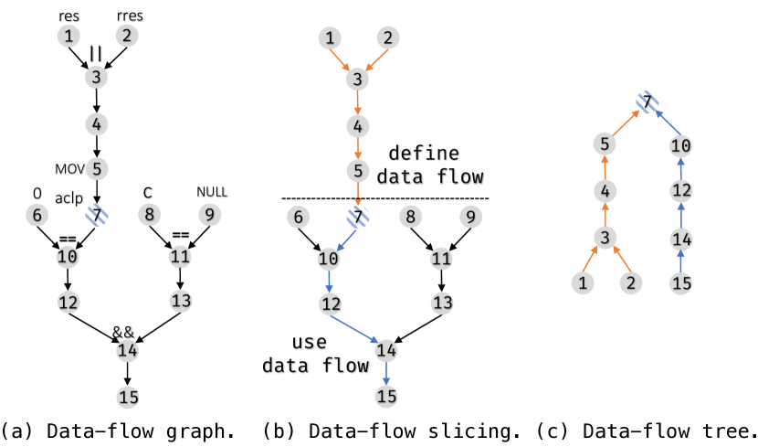
Figure 1: Data-flow graphs and tree built from the execution trace of 2. Define/use-data flows to construct data-flow tree are obtained through data-flow slicing.

Edge Features.Edge FeaturesEdge Features?Edge FeaturesEdge Features. We define four different kinds of edges to represent different relationships. Specifically, $d$-edge describes the explicit data flow; $i$-edge represents the implicit data flow; $c$-edge indicates the local control dependency; and $r$-edge defines the redefinition relationship. The $d$-edge and $i$-edge are straightforward, and we can simply add such edges to nodes that contain such relationships. A $c$-edge connects a $v$-node of a conditional variable and a $o$-node of the comparison instruction. We design $r$-edges to indicate whether two or more live-variables belong to the same source-level variable.

⬇

1 res = (res || rres);

2 aclp = res; // value is passed through function return

3 if (c == NULL && aclp == 0){ ... }

Code 2: Operations on critical data aclp in proftpd.

2 shows some operations related to the critical variable aclp. Figure 1 (a) shows a data-flow graph generated from the execution of 2. In the data-flow graph, node 1-5 and 7 are generated from operations of code in line 1 and line 2. Node 6 and 8-15 are generated from operations of code in line 3. Among these all the nodes, node 3, 5, 10, 11, and 14 are $o$-nodes, and others are $v$-nodes.

IV-C Dataset Generation

A deep-learning based approach requires a certain amount of labeled data to produce an effective model. However, we have not seen such a large dataset of critical data available. Although existing works rely on human efforts to annotate critical data, the manual analysis is not only time-consuming but also prone to inaccuracies, like missing critical variables or including non-critical ones. To solve this problem, we decide to utilize the program source code to help label variables. Specifically, we first label variables in the source code, and use a customized compiler pass to deliver the label information from the source code to the binary. With a simple static binary analysis, we can identify labeled data and thus construct the large-scale dataset. Please note that the source code is only used for preparing the dataset. Our approach, including model training and application, will not require any source code.

Semi-automatic Data Labeling.Semi-automatic Data LabelingSemi-automatic Data Labeling?Semi-automatic Data LabelingSemi-automatic Data Labeling. Although it is relevantly easier to identify variables from the source code, a certain amount of human efforts is still needed. We develop several heuristic-based rules to assist the critical-data labeling. These rules help pinpoint candidate variables, and then we manually check the context to confirm the criticalness. It is worthwhile to mention that the semi-automatic method used in this section are not complete, which means it may miss some critical data. We believe this is not a big problem since we merely use it for labeling and generating training data for the deep learning algorithm.

Manual Critical-data Confirmation.Manual Critical-data ConfirmationManual Critical-data Confirmation?Manual Critical-data ConfirmationManual Critical-data Confirmation. Once the heuristic-based method provides a set of candidate critical data, we rely on human efforts to confirm each of them. In particular, we consider two concrete scenarios that use critical variables. First, a variable is useful to grant attackers extra privileges, such as authentication flags and security configurations [67]. 1 provides one example, which is simplified from the real-world program proftpd. Corrupting this data will allow malicious attackers to bypass the authentication even without correct credentials. Second, a variable contains sensitive information that can be used to launch next-step attacks. For example, attackers can use the HeartBleed vulnerability to steal private keys of public services, which enables them to force well-known web sites [1]. Other examples include password, stack canary [19] and runtime code addresses [20]. We confirm the candidate variable is critical when the manual inspection reveals such usages. If one candidate does not belong to either of two cases, we label it as a negative sample (i.e., non-critical data).

Data-flow Graph Generation.Data-flow Graph GenerationData-flow Graph Generation?Data-flow Graph GenerationData-flow Graph Generation. To build the dynamic data-flow graph, we develop a Pin tool to collect various runtime information [40], including executed instructions and accessed memory addresses. Then, we analyze the execution trace offline to track the liveness of variables. The liveness of global variable is straightforward and does not need further analysis. For stack variables, we use the stack allocation at function entry and deallocation at function exit to indicate their lifetime. For heap variables, we track the memory allocation (e.g., using malloc) and deallocation (e.g., using free) by hooking all heap management functions. Whenever a stack frame or a heap chunk is deallocated, we mark the freed region so that future accesses to this region create new variables. Once the analysis is done, building the data-flow graph is quite straightforward. Therefore, we skip the details in our paper.

There are several ways to pass the variable labels from the source code to the binary. In our implementation, we insert some redundant instructions that encode variable labels to binary code during compiling. We identify and remove these redundant instructions from the execution trace, in order to avoid introducing extra code patterns of critical variables.

Measuring Global Control Dependency.Measuring Global Control DependencyMeasuring Global Control Dependency?Measuring Global Control DependencyMeasuring Global Control Dependency. We develop a tool to measure the global control dependency of each variable.

1. The tool recompiles the target program and assigns a random ID for each basic block.

2. (dry-run) The tool run the program with a given input. Meanwhile, it records the distinct executed basic blocks.

3. (flipped-run) The tool runs the program again with the same input, but flips the interested variable (say $v_{i}$) before the use. It records the executed basic blocks in this run.

4. By comparing the triggered basic blocks of two runs, the tool counts the number ($n$) of different basic blocks.

The number $n$ is the measurement of global control dependency for variable $v_{i}$. We admit that one flip is not always effective to trigger another branches for some case, therefore, we flips several time of such variables and choose the max $n$ as the measurement. If $n$ is larger than a predefined threshold $\theta$, $v_{i}$ is one candidate critical variable. Once the manual inspection confirms the criticalness, we will attach $n$ to $v_{i}$’s $v$-node in the data-flow graph as a node feature.

Dataset Statistics.Dataset StatisticsDataset Statistics?Dataset StatisticsDataset Statistics. Through the automatic tool and some human efforts, we finally generate a dataset (shown in Table I) that involved six programs : bftpd, ghttpd, telnet, vsftpd, proftpd, and nginx. The six data-flow graphs generated from the execution traces contain 117 critical variable and 104 non-critical variables in source code. To the best of our knowledge, this is the first dataset containing so many labeled critical variables. We will release the dataset to boost the research on critical variables. Noting that in programs, the number of non-critical variables is larger than critical variables. However, lots of them can be easily filtered out. Therefore, in order to train a high quality model, we always choose non-critical variables that similar to critical variables to add to our dataset.

TABLE I: Dataset statistics, including numbers of labeled critical variables and non-critical variable in each program.

	nginx	bftpd	proftpd	ghttpd	telnet	vsftpd	total
Critical	12	28	23	5	11	19	117
Non-Critical	13	18	28	3	10	32	104

V A Straightforward Method

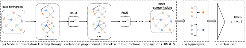
Figure 2: Graph neural network based model. Red and blue colors mark live-variable nodes belonging to two variables. A $n$-layer GNN learns representations for nodes simultaneously; A aggregator aggregates node representations; A classifier predicts variable labels.

Given the raw data in a graph structure, the straightforward way to solve this problem is to adopt a Graph Neural Network (GNN [71]). In this section, we present our first design to solve the critical variable identification problem.

V-A Overview

Since a variable instance in the execution trace corresponds to several live-variables, one data sample is a set of live-variable nodes in the data-flow graph. Therefore, we take features of these live-variable nodes as input for classification.

With the graph structure and its nodes and edges, graph analysis tasks can be grouped into three categories [65]: graph classification, node classification, and link prediction. Although in principle, node classification, which aims to classify nodes in graph into different categories, is suitable for our problem, we notice they are still not exactly the same. Because whether a variable is critical or not is based on all its defines and usages (corresponding to one or several live-variable nodes in graph). A good representation learned for a variable must take all its live-variables and surrounded data flows into consideration. However, a node representation learned by a graph neural network can only aggregate local node features and graph structure around the node. Therefore, our model to learn must aggregate features from all its live-variables.

To learn good representation for variables, we proposed a model design based on the graph neural network (as shown in Figure 2). The designed model consists of three components: node representation learning, node representation aggregation and variable classification. Firstly, the graph neural network helps to learn representations for each live-variable in a data-flow graph. Secondly, the a aggregator was adopt to aggregate features from several node representations learned for live-variables that belongs to the same real-world variable. Thirdly, a classifier will classify variables into two categories (critical, not-critical) based on the aggregated results.

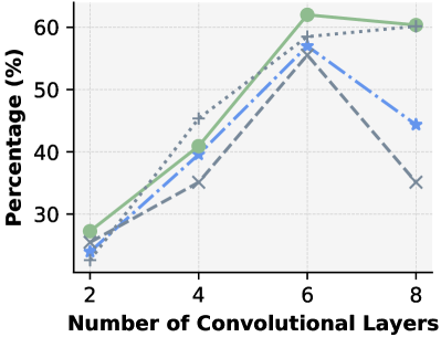
(a) Results of BRGCN

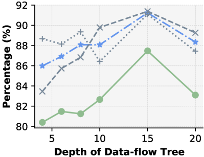
(b) Results of Tree-LSTM

Figure 3: Comparison between the straightforward method and non-intuitive method. We perform the evaluation with different number of layers and flow depths to find the optimal design choice.

V-B Model

Firstly, in node representation learning, we adopt the Relational Graph Convolutional Network with Bi-directional Propagation (BRGCN [64]) to learn node representations for each node in the graph. Generally, the main idea of graph convolutional network (massage passing GNN) is to generate a node $v_{i}$’s representation by aggregating its own features $\mathbf{h}_{i}$ and neighbors’ features $\mathbf{h}_{j}$, where $v_{j}\in$ set of neighbors of $v_{i}$. Specifically, the propagation rules of BRGCN are defined as:

$$\begin{split}h_{i}^{(l+1)}&=\sigma\left(\sum_{r\in\mathcal{R}}\left(\sum_{j\in\mathcal{IN}_{i}^{r}}\frac{1}{c_{i,r}}W_{r}^{in(l)}h_{j}^{(l)}+\right.\right.\\ &\left.\left.\sum_{k\in\mathcal{OUT}_{i}^{r}}\frac{1}{c_{i,r}}W_{r}^{out(l)}h_{k}^{(l)}\right)+W_{0}^{(l)}h_{i}^{(l)}\right)\end{split}$$ (1)

where $\mathcal{IN}_{i}^{r}$ and $\mathcal{OUT}_{i}^{r}$ denote the set of incoming neighbors and outgoing neighbors for node $i$ under the relation $r\in\mathcal{R}$, respectively. The proposed dynamic data-flow graph contains 4 kinds of relation (i.e., 4 types of edges) among nodes in graph. $W_{r}^{d(l)}$ is relation-specific transformations matrix for relation $r$, which enables relation-specific message passing, thus preserving edge type relationship, where $d$ represent the direction of an edge. $c_{i,r}$ is a normalization constant that we set as the count of neighbor relation $r$ for node $i$. To ensure that the representation of a node at layer $l$ + 1 can also be informed by the corresponding representation at layer $l$, a single self-connection (i.e., $W_{0}^{(l)}$) term is added. All messages passed along with incoming and outgoing edges are aggregated through an element-wise activation function $\sigma(\cdot)$.

For each node, its old features ($h_{i}^{(l)}$) and its neighbors’ old features ($h_{j}^{(l)}$) are passed along with the edges ($\left(v_{i},r,v_{j}\right)\in\mathcal{E}\lor\left(v_{j},r,v_{i}\right)\in\mathcal{E}$), and then aggregated through a normalized sum ($\sum(\cdot)$) and an activation function ($\sigma(\cdot)$) to get the updated new features ($h_{i}^{(l+1)}$). $W_{r}^{d(l)}$ and $W_{0}^{(l)}$ are the parameters to be learned. By stacking $k$-layers of RGCN together, the representation of node $v_{i}$ could capture the $k$-hop local graph information centered at node $v_{i}$. Besides, the different sets of weights $W_{r}^{d(l)}$ for different types of edges and sum-aggregation adopted in Equation 1 can help learn the graph structures corresponding to information flow. With different graph structures and node features, the network can learn some local dataflow features (with in $k$-hop) around a live-variable.

Basically, we choose BRGCN mainly due to its two features: 1) BRGCN can learn different types of edges in graph, which is preferred by us. 2) the bi-directional propagation can better learn the data-flow features through bi-directional propagations, which has been proved by previous research in experiments [64].

Secondly, after BRGCN learned node representations for each live-variable, that belongs the the same real-ward variable. A aggregator was adopted to aggregate node representations of the variable’s all live-variables. In our experiments, we adopt the max-pooling achieves this purpose. The max-pooling can be defined as:

$$\begin{split}\hat{h^{r}}=\max_{i\in\mathbf{V}_{k}}\left(h_{i}^{(k)}\right)\end{split}$$ (2)

where $\mathbf{V}_{r}$ denotes all live-variables nodes of variable $r$ in graph. $h_{i}^{(k)}$ is the node representation learned by a $k$-layer BRGCN. The $\max$ pooling will calculate the max value of each hidden states of node representations in $\mathbf{V}_{r}$.

Finally, a output layer for predicting variable labels ($\hat{y}\in{0,1}$) can be formalized as:

$$\hat{y}=\sigma\left(\hat{h^{r}}*A^{T}+b\right)$$ (3)

which contains a linear transformation on the learned representation $\hat{h^{r}}$ for variable $r$ and an activation function $\sigma$.

V-C Experiment and Results

To evaluate the effectiveness of the proposed model based on BRGCN, we train the neural network with different number ($k$) of layers in BRGCN. Basically, the number of layers in BRGCN represents the length of the paths (in the data-flow graph) whose path-level features are considered in node representation learning.

Figure 3 (a) shows the model performance with different numbers of layers. We get the following observations from the experiments: Observation 1: The best model performance (62.00% accuracy and 0.5698 F1 score) appears when the number of layers is 6. Observation 2: When the number of layers is less than 6, the model will perform better when increasing the number of layers in BRGCN model. Observation 3: However, when the number of layers is larger than 6, the model performs worse when increasing the number of layers in BRGCN model.

V-D Lessons Learned

Based on our domain knowledge, we found that “shallow” BRGCN models (i.e., with 6 or less layers) are not really suitable for distinguishing critical variables from non-critical ones. For example, a critical variable could be firstly passed as a parameter across different functions before it is involved in any meaningful operations. In such cases, the data flow(s) near the live-variable nodes are resulted from data-transfer operations, which do not hold any useful feature information about the critical variable. Therefore, only when learning features from a longer data-flow path, a model could become capable in identifying such critical variables. Obviously, a BRGCN model with $6$-layers can only learn nearby data-flow features. Hence, it is not very surprising that the accuracy achieved by the best BRGCN model is only 62%.

Why is BRGCN not capable to learn features carried by long data-flow paths? Firstly, based on the literature, we notice that over-smoothing is a common issue faced by a GNN, which means that the learned node representations of different classes would become indistinguishable when the model is stacking multiple layers [12]. Specifically, as the over-smoothing effect happens when the graph convolution architecture becomes deep, the 6-layer GNN used in [63] will wash out much useful information in the representation. Secondly, besides the widely-known limitations of GNN models, we have some new insight regarding why BRGCN cannot learn useful features from long data-flows path. Although bi-directional propagation in BRGCN could help a model learn more data-flow features for some nodes, as shown in [64], it will result in a huge amount of loop in the message propagation path due to its characteristic of passing messages in both directions. Figure 4 shows the message proportion process when learning the node representation for node $7$ (i.e., node for variable aclp) in the data-flow graph (as shown in Figure 1) through a $3$-layer BRGCN as defined in Equation 1. For example, in layer $1$ the updated hidden states $h_{7}$ aggregates features from node $7$, node $5$ and node $10$. In the 31 propagation paths shown in the figure, node $5$’s and node $10$’s input features can be propagated to node $7$ along with 6 and 7 aggregation paths, respectively. However, node $14$’s input feature can only be propagated to node $7$ along with 1 aggregation path. In such a case, it is more likely that the learned representation for node $7$ aggregates more features from node $5$ and node $10$ than from node $14$. We can easily draw the conclusion that as the distance between a node and the target node increases, the “influence” of the node on the target node exponentially decreases in node representation learning. Therefore, the model can hardly learn features from nodes far away in the data-flow path. This can explain why the model performance drops tremendously when the number of layers reaches 6 in our experiments.

Figure 4: Message propagations when learning node-$7$’s representation in the data-flow graph shown in Figure 1 through a $3$-layer BRGCN.

VI A Non-Intuitive Method

Based on the lessons learned from the straightforward method, we propose a non-intuitive method to significantly improve the performance of critical variable identification. Since the straightforward method cannot learn useful features from long data-flow paths, a key idea of the new method is to enable the neural model to gain this important capability.

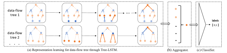
Figure 5: Tree-LSTM based model. A Tree-LSTM learns representations for each of a set of data-flow trees that corresponding to one real-world variable. An aggregator aggregates tree representations; A classifier will predict the variable labels.

VI-A How to Learn Features Carried by Long Data-Flow Paths?

In sequence models, the vanilla RNN naturally struggles to remember information for long sequences because it suffers from derivative vanishing and explosion problem [26]. Long Short-term Memory (LSTM [27]) networks were proposed to deal with these problems by introducing new gates and states, which allow for a better control over the gradient flow and enable better preservation of “long-term dependencies”.

Thus, it should be helpful if we adopt a LSTM cell in a GNN (e.g., Graph LSTM [38]). However, having lots of loops in BRGCN’s propagation paths is still a challenge that restricts the model’s ability to learn features carried by long data-flow paths. Hence, we must find a way to eliminate loops in propagation paths, while reserving the model ability to learn data-flow features in a bi-directional manner. Therefore, the problem boils down to on thing: whether we can eliminate loops in propagation paths while preserving most of the data-flow features. To solve this problem, we propose the design of data-flow trees to represent a variable’s data-flow in a tree structure, and adopt a Tree-LSTM based model to learn data-flow features from such a tree data structure. We note that although such a tree structure is non-intuitive from the viewpoint of classical data-flow analysis, it can make the critical variable identification problem significantly more likely to be solved through deep learning.

VI-B A Non-Intuitive Data Structure – Data-Flow Tree

In this section, we will discuss how to convert data flow in a graph structure around a live-variable into a tree structure, while keeping important data-flow features.

Data-flow Slicing. Given the enhanced data-flow graph as defined in § IV-B, we generate a data-flow tree for each live-variable in the graph. For each variable used in program execution, we notice two most important kinds of data flows:

1. Define-Flow, which is the data flow that calculate a value assigned to the variable.

2. Use-Flow, which is the data flow that use the value of the variable.

Taking 2 as example, line 1 and line 2 are code to calculate the value that will be stored into the variable aclp. Therefore, the data flow resulted from the execution of these two lines of code are define-flow. And line 3 is code that use the value of this variable. Therefore, the data flow resulted from the execution of this line of code are use-flow.

It should be noticed that there may exist several define-flow and use-flow for one variable, because a variable may be assigned and used several times in one execution. Each define-flow and use-flow are corresponding to one live-variable. The terminology of “define-use” pairs in program analysis is just used to reflect such relationship.

Define-flow and use-flow can be identified from the whole data-flow graph through backward and forward data-flow slicing. Choosing one live-variable node as root node in the data-flow graph, we can firstly include all the nodes and edges that can be reached through forward data-flow tracking within $k$ steps. And the generated sub-graph represents the $k$-hop use-flow. Then, we can include all the nodes and edges that can be reached through backward data-flow tracking within $k$ steps. And the generated sub-graph represents the $k$-hop define-flow. The orange color and blue color paths in Figure 1 (b) demonstrate the define-flow and use-flow of live-variable aclp (generated from backward and forward data-flow tracking), respectively. Besides, there is one strategy that we adopt in our slicing algorithm to avoid loops. That is, we simply remove an edge if adding the edge will result in a loop.

After collecting the define-flow and use-flow sub-graphs, we rotate the direction of the edges in the use-flow sub-graph and assign the rotated edges with a different type, so that define-flow and use-flow are distinguishable. Figure 1 (c) shows the data-flow tree generated through the above-described graph processing. The live-variable node, for which we want to learn a representation, is the root node of the data-flow tree. The other nodes in the define-flow and use-flow sub-graphs are the leaves in the tree. Noting that since a source code variable is corresponding to a set of live-variables in data-flow graph. Therefore, we will generate a set of data-flow trees for each variable, and these data-flow trees could share some nodes.

Similar to a enhanced data-flow graph, a node in our data-flow tree structure includes instruction opcodes or measured control dependencies as node features. Besides, we notice that each edge is only corresponding to one leaf node in the tree structure, which allows us to simply encode the edge type information as a node feature in the corresponding leaf node. By encoding edge type information as a node feature, we can reduce the number of parameters in model design. Finally, since the data-flow paths of some variables could be very long, we set up a threshold ($k$) during data-flow slicing so that the depth of each data-flow tree can be bounded.

VI-C Overview

Since, one variable instance is corresponding to several live-variables, one data sample in our dataset is a set of data-flow tree and each data-flow tree is generated from on live-variable.

Given the newly-designed data-flow tree, we adopt Tree-LSTM [59] as backbone to design our model. Figure 5 shows the whole workflow of our design. Similar to the BRGCN model in the straightforward method, the Tree-LSTM based model also consists of three components: representation learning of data-flow tree, tree representation aggregation and variable classification. Each component achieves a similar purpose as that in the straightforward model design. The only difference is how we design the first component.

VI-D Design

The message-passing order of Tree-LSTM is a significantly difference from models such as graph neural networks, where all nodes are pulling messages from upstream ones simultaneously. As shown in the Figure 2, the BRGCN model learning representation for each nodes simultaneously. In the case of Tree-LSTM, messages start from leaves of the tree, and propagate/processed upwards until they reach the roots. Figure 5 (a) shows the message-passing process of Tree-LSTM on two data-flow trees. The message-passing process will end on the root node, and the learned representation of root node essentially can aggregate features from all leaves of a data-flow tree. We appendix the formulas of message-passing function in Child-Sum Tree-LSTM in the appendix (Appendix A).

After Tree-LSTM enable us to learn a representation for a live variable, that incorporates its define-flow and use-flow, we adopt the pooling layer to generate the variable representation by aggregating representation of each root nodes corresponding to live-variable, and a output layer to predict the label of variable based on the aggregated results. Since, the design of pooling layer and output layer in the Tree-LSTM based model is similar to that in the BRGCN based method, we will not cover the details here.

VI-E Reflection Remarks

A LSTM network designed on top of data-flow trees has four main benefits. Benefit 1: since the neural network will propagate the information from leave nodes to the root node, the learning algorithm can guarantee that all node features and most edge features in define-flow and use-flow will be propagated to the learned live-variable representation. Benefit 2: the different edge types can enable the neural network to distinguish define-flow from use-flow. Benefit 3: All nodes in the tree only appear in one propagation path. Benefit 4: The adopted LSTM cell enables the model to learn features carried by long data-flow paths. While the BRGCN based model design can only enjoy Benefit 1 and Benefit 2, the Tree-LSTM based model design can enjoy all of the four benefits.

Lastly, despite these advantages, we admit that our design has one limitation: the removal of some edges to avoid loops could result in loss of some data-flow features. However, considering that the BRGCN model can only learn features carried by a very short data flow, we believe that the benefits of the Tree-LSTM based model are worth such a feature loss.

VII Evaluation

In this section, we aim to answers four questions: ➀ Can our method identify critical data? ➁ What are the impacts of model depth, type of pooling layer, control dependency on model performance? ➂ Is the proposed method better than the baselines? ➃ Is the proposed method efficient?

Dataset.DatasetDataset?DatasetDataset. As mentioned in § IV, we labeled 117 critical variables and 104 non-critical ones in 6 programs, respectively. To generate the dataset, through $15$-hop data-flow slicing on 6 enhanced data-flow graphs (one such graph from each program) we obtained 862 variable usage instances which consist of 145,860 nodes and 133,668 edges in total. When a local variable is created and destroyed $n$ times during one program execution, we should view it as $n$ different variable usage instances. Since some of the labeled variables are local variables, which could be created and destroyed every time the corresponding function is called and returning, the number of variable usage instances is larger than the number of labeled variables. Therefore, even though we do not have a lot of labeled variables, we can still generate a number of distinctive data samples for training. On average, each variable usage instance (i.e., data sample) consists of 25.22 live-variables, and each live-variable corresponds to one data-flow tree.

Model Training.Model TrainingModel Training?Model TrainingModel Training. During embedding, each data sample must be firstly converted to a feature vector. Accordingly, the opcode types and the edge types, which are encoded as an integer in a data-flow tree, are converted to a feature vector. Then, we append the measured control dependencies (an integer value ranging from -1 to 0xffff) to the feature vector.

Running the deep learning algorithm with such feature vectors, we have trained and tested 6 different neural models. Table II shows the average accuracy, precision, recall, and F1 scores for the 6 neural models as a whole. Specifically, after all of the 6 neural models are tested, we firstly count the total numbers of true positives, true negatives, false positive, and false negatives in testing set, respectively. Then we calculate the average accuracy, precision, recall, and F1 scores.

To train each model, we let the data samples obtained from 5 programs be the training set, and the data samples from the remaining 1 program be the testing set. In this way, each trained model is always tested on a previously unseen program. Since there are 6 options when we choose the 5 training programs, there are in total 6 neural models to train. Compared to training only one model, our training and testing strategy can fully leverage the data samples we have obtained and avoid the randomness introduced by dataset splitting. We train each model for 50 epochs on a machine with 40 Intel(R) Xeon(R) CPU E5-2650, and 64GB memory. On average, it takes 521.35 seconds to train a model for one epoch.

Evaluation Metrics.Evaluation MetricsEvaluation Metrics?Evaluation MetricsEvaluation Metrics. We use 4 widely-used metrics to evaluate our models: accuracy, precision, recall, and F1 score. The higher the accuracy and F1 score are, the better the model performs in providing good prediction results. Since the accuracy metric is misleading for imbalanced datasets, we also measure F1 scores. We measure the precision and recall to evaluate each model’s false positives and false negatives.

TABLE II: Evaluation results on our model and other baselines.

Design	Model	Accuracy	Precision	Recall	F1
Ours	Tree-LSTM	0.8747	0.9108	0.9138	0.9123
Baseline 1	RNN	0.7254	0.8287	0.6342	0.7185
Baseline 2	LSTM	0.7465	0.8484	0.6871	0.7593
Baseline 3	MLP	0.2590	0.3900	0.3821	0.3859
Baseline 4	ConvGNN	0.5465	0.5071	0.3580	0.4197
Baseline 5	BRGCN	0.6200	0.5849	0.5553	0.5698

VII-A Can Our Method Identify Critical Data?

After we trained 6 models and tested them on 6 previous unseen program, the results in Table II show that our model overall can achieve 87.47% accuracy, 91.08% precision, 91.38% recall and a F1 score of 0.9123. Specifically, our model successful identified 562 out of 615 critical variable usages. 55 non-critical variable usages were misclassified as critical. Compared to the straightforward method, which achieved 62.00% accuracy and a F1 score of 0.5698 on the same dataset, the non-intuitive method is significantly better.

To show a practical use case, we choose proftpd, which is a large server program, as an example. Firstly, we identified 1,231 conditional branches in one execution trace. By flipping the corresponding conditional variables, we found 794 conditional variables that resulted in varied triggered basic blocks (i.e., measurement of control dependency). We randomly selected 30 variables from these 794 conditional variables and generated a set of data-flow trees for each of them. Then, we fed the data-flow trees to the model and got the prediction results, i.e., 13 positives and 17 negatives. Through manually verifying each variable, we found that 12 of 13 are true positives, and that 16 of 17 are true negatives.

Regarding the variation among the 6 test programs, we found that the testing results against 5 out of the 6 programs are good, but there is one outlier. When we used vsftpd as the test program, results shown that there are many false positives and thus very low precision score (30%). When we inspect the data flow of such false positives, we found some characteristics did not appear in any negative samples in the training set. Though we use the same criteria for labeling, it happens that vsftpd contains some non-critical flags, whose value are loaded from configuration files (e.g., network configuration), and would result to new execution path when being flipped. Since in the training phase, the model did not see any other non-critical samples that present such characteristics in the other 5 programs. Therefore, it is reasonable the trained model misclassify this category of non-critical variables. Besides, We will show details of some cases in case study (§ VIII).

VII-B Impacts of Design Choices

We want to answer three questions related to model design: 1) Can the Tree-LSTM based model learn features carried in long data-flow paths? 2) Whether different pooling layers will lead to different model performance? 3) What is the impact of measured control dependencies on model performance?

Firstly, we generate data-flow trees with different depth $k$ through data-flow slicing. In this way, we can evaluate the impact of tree depth on model performance. Figure 3 (b) shows the corresponding result. Basically, we get two observations: Observation 1: the model reaches best performance when the tree depth is 15. Observation 2: the overall model performance is better than that of GNN-based models. Based the these observations, we can conclude that the proposed Tree-LSTM based model can learn features carried by a data-flow path which is as long as 15, which is much better than what a GNN-based model could do. The results show that the Tree-LSTM based design can avoid the over-smoothing issues when learning features carried by long data-flow paths.

Secondly,to answer the second question, we evaluate the model performance with Max-Pooling (the default setting), Average Pooling and Sum Pooling. Table III shows the model performance with different pooling layers. Regarding why Average Pooling and Sum Pooling are worse than Max Pooling, we conjecture that the important features of critical variables only exist in a subset of the relevant data flows. Max Pooling can highlight these features in many data flows of a critical variable, while Sum Pooling and Averaging Pooling could smooth out such useful features.

TABLE III: Model performance with different pooling layers.

Design	Accuracy	Precision	Recall	F1
Max Pooling	0.8747	0.9108	0.9138	0.9123
Average Pooling	0.8008	0.9014	0.8330	0.8659
Sum Pooling	0.7716	0.90767	0.7837	0.8411

Thirdly, to answer question 3), we run one experiment to evaluate the model performance without measured control dependencies as a feature. We present the model performance under different settings in Table IV. The experiment results show that without measured control dependency, the model accuracy suffers from 3.72% degradation. This shows the effectiveness of measured control dependencies.

VII-C Is the Proposed Method Better than Meaningful Baselines?

We compare our work with five baselines. Since there are no other work that directly solve the critical variable identification problem, we borrow some popular deep-learning methods adopted to solve some other security analysis tasks as a baselines. Specifically, previous (binary level security analysis) work usually adopt an instruction sequence as input, and a sequence model (RNN, LSTM) as backbone. Accordingly, we adopt 2 sequence models as 2 of the 5 baselines.

In baseline 1 and baseline 2, we trace instructions that can be reached through forward and backward taint analysis within $15$-hops from a variable (as taint seed). Then, we adopt a sequence model to predict variable types. Since an instruction sequence data sample is usually longer than 200 bytes, and it is known that RNN and LSTM may not handle long sequences very well, we adopt the hierarchical RNN/LSTM design proposed by DEEPVSA [25], which effectively reduces the length of the sequence which the model will see at each level (hierarchy). In essence, one RNN/LSTM model will be used to embed each instruction into a latent space, and another RNN/LSTM model will process the sequence of embedded instructions. We show the results of RNN/LSTM based models in Table II. Based on the results, we can conclude that the critical variable identification problem cannot be well handled by a RNN/LSTM based models on instruction sequences.

Besides, we adopt 3 other baselines. Firstly, in baseline 3, we adopt a multi-layer perception (MLP) model to directly learn features from live-variable nodes without consider nearby data flow, then adopt a Max-Pooling layer to aggregate learned representations of all live-variable nodes that belong to a variable, finally predict the variable’s type through an output layer. Table II shows that the MLP model has poor performance.

TABLE IV: Model performance with and without control dependency.

Design	Accuracy	Precision	Recall	F1
Ours	0.8747	0.9108	0.9138	0.9123
w/o MCD	0.8375	0.9022	0.8868	0.8944

Secondly, in baseline 4, we adopt a 4 layer ConvGNN and train a model on enhanced data-flow graphs used in the straightforward method. In ConvGNN, all types of edges are treated and processed with the same weight matrix $W$. The model only propagates information in the same direction of each edge. Therefore, all use-flow features (connected by outgoing edges) will not be propagated to corresponding live-variable nodes. The results show that ConvGNN also cannot effectively identify critical variables.

Thirdly, baseline 5 presents the performance of the straightforward method when the number of layer is 6. Compared to all other methods, we find that even though the straightforward method is not as good as the proposed Tree-LSTM based method, it is still better than the other baselines. This indicates that learning from variable data-flow is a most promising method to solve the problem.

VII-D Is the Proposed Method Efficient?

To answer question ➃, we evaluate runtime performance of three main components in our approach. Basically, the proposed approach needs to trace program data flow, build data-flow graph, and infer variable type. Therefore, we report the following information in Table V to reflect the runtime performance of our approach: 1) the runtime performance of data-flow tracing. 2) the time consumption of data-flow graph construction. 3) the time consumption of model inference.

Firstly, the second column in Table V reports the time to trace the data flow in each program execution. Secondly, the time consumption of graph construction largely depends on the size of the generated execution trace. Columns 3-4 in Table V report the size (number of executed instructions) of generated trace and the time consumption to build data-flow graph, respectively. Thirdly, the time consumption of model inference is largely dependent on how many variables to infer. Accordingly, we report the average time that a model processes a variable in each program.

Based on the evaluation results, we can know that building data-flow graph from the execution trace is the most time-consuming step. However, even for proftpd, which is a fairly large server program, our tool can finish building its data-flow graph within 20 minutes.

TABLE V: Performance evaluation, including time and storage cost of data-flow tracing, graph construction, and model inference.

	Tracing	Graph Construction		Inference
	Time (s)	Trace Size(Ins)	Time(m&s)	Time(s)/Per-Var
nginx	12.4	3059335	47.11s	0.3129
bftpd	23.5	85519298	12m38.476s	0.1304
proftpd	45.1	130065689	19m52.295s	0.4077
ghttpd	3.1	600177	9.704s	0.1247
telnet	20.58	514522	8.579s	0.1697
vsftpd	20.58	986613	15.176s	0.2426

VIII Case Study

In this section, we provide our explanation and insights about the model decisions. Note that all the statements made in this section are not general conclusions.

True Positive.True PositiveTrue Positive?True PositiveTrue Positive. We first start with model’s successes. Our model correctly classified the example shown in 1 as a positive example. As explained in § I, variable aclp will carry the information about whether the logging in user is block or not, and attacker can illegally login if the value of the variable is modified during execution. The data flow tree contains the information of the critical operation shown in 2, and our trained model is able to capture that information. Figure 1 (c) only show partial of the data-flow tree, the complete data flow tree is fairly long, and the graph features contain good amount of information. For example, the opcode feature shows that there are several data transfer operations (MOV instructions) and several logical operations. Although not shown in the Fig. Figure 1 (c), there is also a vector operation opcode. The global control dependency is also fairly quite big, which result in 67 changed executed basic blocks. Though it is not possible to explain the reasons of a deep learning model’s decision, it is clear that the information is rich in this example, and heuristically, a variable that is processed by diverse opcodes and with great control dependency is likely to be critical.

True Negative.True NegativeTrue Negative?True NegativeTrue Negative. We also discuss an example that the model correctly identifies non-critical data. The variable daemonmode in bftpd-5.6 controls whether the server should be run as a daemon or not. With careful checks, we believe this variable is non-critical as the program behavior is almost the same when running as daemon or not. The usage of this variable is quite simple: it is initialized with a value from the command line or the configuration file, and then gets checked during the program setting up before spawning the daemon. These usages result in three data-flow trees (partially shown in Figure 6 (a)). The data flows are very short and no fork are presented in these trees. In addition, the global control dependency is only 1, which means that the executed basic blocks are only changed by 1 when this flag is flipped. We believe this is the main reason that our model classifies this variable as non-critical.

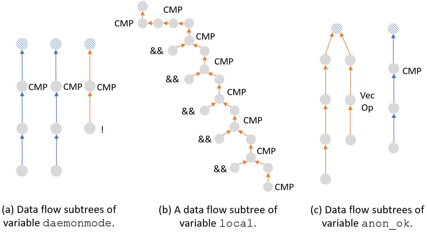
Figure 6: Data flow subtrees for case studies.

False Positive.False PositiveFalse Positive?False PositiveFalse Positive. In this example, our model incorrectly treats one non-critical variable as critical. Specifically, variable local is used in bftpd-5.6 to find the timezone difference between the client and the server, only for security-unrelated operations such as logging. But our model gives the unexpected label. By checking its data flow (partially shown in Figure 6 (b)), we can see that the data flow is complicated, including many comparison operations and logical operations, as finding time zone difference involves many comparisons. The global control dependency is five, indicating this variable can slightly influence the overall program execution. All these facts confuse our model to draw the wrong conclusion. A human analyst can filter this variable out when figuring out that it is not related to security-related operations. However, at binary level there is no comment or name information in the traces. Therefore, in this case the model does not have sufficient information, and thus treats the data flow of a non-critical variable as one of critical variables.

False Negative.False NegativeFalse Negative?False NegativeFalse Negative. Lastly, we examine a case where the model misses a critical variable. anon_ok is a flag indicating whether anonymous logins are allowed. By modifying this flag, attackers can anonymously login to the server, then conduct illegal access or launch deny-of-service attacks. Therefore, this variable should be considered as critical. Figure 6 (c) shows its full define-flow tree (left) and use-flow tree (right). Even though the define-flow tree has a vector operation, and the use-flow tree contains a CMP operation. The whole data flows are fairly short, and the global control dependency is only 17, which could indicate that this variable is not very critical. The reason of this misclassification is similar to the false positive case. When human analyst looks at the variable, it is obvious that the data is related to anonymous login and thus critical. However, the model does not have access to this information at binary level, and if the data-flow graph is appeared to not contain conspicuous features that relevant to critical data, the model is possible to have a misclassification.

IX Related Work

Attacks on Critical Data.Attacks on Critical DataAttacks on Critical Data?Attacks on Critical DataAttacks on Critical Data. Decades ago, Chen et al. demonstrated that data-oriented attacks, which merely modifies several bytes of program memory to launch attacks, are feasible in popular server applications [13]. However, only in very recent years such attacks get attention from both industry [67, 33, 58] and academia [28]. For example, by corrupting the Safemode flag, attackers can run arbitrary malicious code inside the Microsoft Internet Explorer (IE) browser [67], while by replacing the EnableProtectionPtr pointer, attacker can bypass the protection provided by Microsoft EMET [33]. Researchers also explored methods to automatically synthesize this new type of attacks [28]. However, all these projects did not discuss methods to identify critical data. In fact, attackers have to manually locate such data from the program source code or even binaries, which is error-prone and time-consuming. Our paper provides an automatic, scalable way to help identify critical data, which moves one step further towards automatic exploit generation [6].

The concept of data-oriented attack has been generalized to represent any attack that does not alter the program’s control data. For example, Hu et al. proposed data-oriented programming (DOP), which demonstrated that data-oriented attacks are expressive, and can even afford Turing-complete computing [30]. DOP does not rely on byte-level critical data, but uses a large amount of small data-flow snippets, called data-oriented gadgets, to synthesize meaningful attacks. The following work block-oriented programming shows that such attacks can be constructed automatically [31]. Despite the feasibility, DOP and BOP are more challenging than corrupting few bytes of critical data. For example, to emulating a network bot [30], attackers have to send over 700 packages to achieve one meaningful malicious action. Therefore, in this paper, we focus on identifying the byte-level critical data that are more dangerous than general ones.

Defenses on Critical Data.Defenses on Critical DataDefenses on Critical Data?Defenses on Critical DataDefenses on Critical Data. Researchers have proposed a set of defenses aiming to prevent data-oriented attacks. Many solutions add memory safety to unsafe languages, trying to eliminate memory issues to avoid being attacked in the first place [42, 43, 11, 44, 32, 44]. However, enforcing a complete memory safety brings significant runtime overhead, and thus has not been adopted by any commercial production. Instead, researchers propose selective protection to achieve a balance between the security and the usability [50, 48]. However, these methods again take the knowledge of critical data as input. Our approach can help previous defense mechanisms by providing a comprehensive list of critical data that should be put into the protection area. Kernel DFI (kDFI) suggests the same protection model [56]. It relies on the elaborated error code in the Linux kernel to help infer critical data. However, this method only works on open-source systems that contain detailed error code, but cannot handle the tremendous user space applications. Our approach supports any system, no matter their working mode or availability of source code.

Deep Learning for Data-Flow Analysis.Deep Learning for Data-Flow AnalysisDeep Learning for Data-Flow Analysis?Deep Learning for Data-Flow AnalysisDeep Learning for Data-Flow Analysis. Wang et al. proposed to solve binary-level security problems through a graph neural network assisted data-flow analysis [64]. Basically, they designed a novel data structure called DFG+ to represent a program’s dynamic data flow and some other features (e.g., variable adjacency), and a graph neural network (so called Bi-directional Relational Graph Convolutional Network (BRGCN)) to learn variable access patterns. Through the learned representations, they were able to find silent buffer overflow in binary execution trace by distinguishing vulnerable buffer accesses and benign accesses. Both their design of data structure, and proposed model are not suitable for the critical variable identification problem because the DFG+ did not incorporate features relevant to our problem and the design of BRGCN cannot learn features carried by long data-flow paths.

X Conclusion and Future Work

In this work, we investigate the application of deep learning to critical data identification. This work provides non-intuitive understanding about (a) why straightforward ways of applying deep learning would fail, and (b) how deep learning should be applied in identifying critical data. Based on our insights, we have discovered a non-intuitive method which combines Tree-LSTM models and a novel data-flow tree data structure to effectively identify critical data from execution traces. The evaluation results show that our method can achieve 87.47% accuracy and a F1 score of 0.9123, which significantly outperform the baselines.

As mentioned in § VI and § VII, this work still has some limitations. Firstly, the designed data-flow tree removes some edges in define-flow and use-flow to avoid loop, which could result in some feature loss. Secondly, our model currently cannot handle some outlier, e.g., some cases in vsftpd. How to include such edge features in data-flow tree and handle these outliers need further investigation and we will try to address these limitations in future work.

Appendix A Child-Sum Tree-LSTM

Given a tree, let $\mathcal{C}{j}$ denote the set of children of node $j$. The Child-Sum Tree-LSTM message-passing function is defined as:

$$\tilde{h}_{j} =\sum_{k\in\mathcal{C}(j)}h_{k},$$ (4)

$$i_{j} =\sigma\left(W^{(i)}x_{j}+U^{(i)}\tilde{h}_{j}+b^{(i)}\right)$$ (5)

$$f_{jk} =\sigma\left(W^{(f)}x_{j}+U^{(f)}h_{k}+b^{(f)}\right)$$ (6)

$$o_{j} =\sigma\left(W^{(o)}x_{j}+U^{(o)}\tilde{h}_{j}+b^{(o)}\right),$$ (7)

$$u_{j} =\tanh\left(W^{(u)}x_{j}+U^{(u)}\tilde{h}_{j}+b^{(u)}\right)$$ (8)

$$c_{j} =i_{j}\odot u_{j}+\sum_{k\in\mathcal{C}(j)}f_{jk}\odot c_{k}$$ (9)

$$h_{j} =o_{j}\odot\tanh\left(c_{j}\right),$$ (10)

As in standard LSTM units, each Tree-LSTM unit (indexed by $j$ ) contains input and output gates $i_{j}$ and $o_{j}$, a memory cell $c_{j}$ and hidden state $h_{j}$. The difference between the standard LSTM unit and Tree-LSTM units is that gating vectors and memory cell updates are dependent on the states of possibly many child units. Additionally, instead of a single forget gate, the Tree-LSTM unit contains one forget gate $f_{jk}$ for each child $k$. This allows the Tree-LSTM unit to selectively incorporate information from each child.

References

- [1] “The HeartBleed Bug,” https://heartbleed.com/, 2015.
- [2] M. Abadi, M. Budiu, U. Erlingsson, and J. Ligatti, “Control-flow Integrity,” in Proceedings of the 12th ACM Conference on Computer and Communications Security, 2005.
- [3] M. Allamanis, M. Brockschmidt, and M. Khademi, “Learning to represent programs with graphs,” arXiv preprint arXiv:1711.00740, 2017.
- [4] Android, “Android Control Flow Integrity,” https://source.android.com/devices/tech/debug/cfi, visited on August 6, 2021.
- [5] T. M. Austin, S. E. Breach, and G. S. Sohi, “Efficient Detection of All Pointer and Array Access Errors,” in Proceedings of the ACM SIGPLAN 1994 Conference on Programming Language Design and Implementation, 1994.
- [6] T. Avgerinos, S. K. Cha, B. L. T. Hao, and D. Brumley, “AEG: Automatic Exploit Generation,” in Proceedings of the 18th Annual Network and Distributed System Security Symposium, 2011.
- [7] D. Bigelow, T. Hobson, R. Rudd, W. Streilein, and H. Okhravi, “Timely Rerandomization for Mitigating Memory Disclosures,” in Proceedings of the 22nd ACM SIGSAC Conference on Computer and Communications Security, 2015.
- [8] A. Bittau, A. Belay, A. Mashtizadeh, D. Mazières, and D. Boneh, “Hacking Blind,” in Proceedings of the 35th IEEE Symposium on Security and Privacy, 2014.
- [9] T. Bletsch, X. Jiang, V. W. Freeh, and Z. Liang, “Jump-Oriented Programming: A New Class of Code-reuse Attack,” in Proceedings of the 6th ACM Symposium on Information, Computer and Communications Security, 2011.
- [10] E. Bosman and H. Bos, “Framing Signals - A Return to Portable Shellcode,” in Proceedings of the 35th IEEE Symposium on Security and Privacy, 2014.
- [11] M. Castro, M. Costa, and T. Harris, “Securing Software by Enforcing Data-Flow Integrity,” in Proceedings of the 7th Symposium on Operating Systems Design and Implementation, 2006.
- [12] D. Chen, Y. Lin, W. Li, P. Li, J. Zhou, and X. Sun, “Measuring and relieving the over-smoothing problem for graph neural networks from the topological view,” in Proceedings of the AAAI Conference on Artificial Intelligence, vol. 34, no. 04, 2020, pp. 3438–3445.
- [13] S. Chen, J. Xu, E. C. Sezer, P. Gauriar, and R. K. Iyer, “Non-Control-Data Attacks Are Realistic Threats,” in Proceedings of the 14th USENIX Security Symposium, 2005.
- [14] Chromium Project, “Chromium Control Flow Integrity,” https://www.chromium.org/developers/testing/control-flow-integrity, visited on August 6, 2021.
- [15] Z. L. Chua, S. Shen, P. Saxena, and Z. Liang, “Neural Nets Can Learn Function Type Signatures from Binaries,” in 26th USENIX Security Symposium (USENIX Security 17), 2017, pp. 99–116.
- [16] J. Chung, C. Gulcehre, K. Cho, and Y. Bengio, “Empirical evaluation of gated recurrent neural networks on sequence modeling,” arXiv preprint arXiv:1412.3555, 2014.
- [17] Clang Project, “Clang Control Flow Integrity,” https://clang.llvm.org/docs/ControlFlowIntegrity.html, visited on August 6, 2021.
- [18] M. Corporation, “Control Flow Guard,” https://msdn.microsoft.com/en-us/library/windows/desktop/mt637065(v=vs.85).aspx, 2016.
- [19] C. Cowan, C. Pu, D. Maier, J. Walpole, P. Bakke, S. Beattie, A. Grier, P. Wagle, Q. Zhang, and H. Hinton, “Stackguard: automatic adaptive detection and prevention of buffer-overflow attacks,” in USENIX security symposium, vol. 98. San Antonio, TX, 1998, pp. 63–78.
- [20] I. Evans, S. Fingeret, J. Gonzalez, U. Otgonbaatar, T. Tang, H. Shrobe, S. Sidiroglou-Douskos, M. Rinard, and H. Okhravi, “Missing the point (er): On the effectiveness of code pointer integrity,” in 2015 IEEE Symposium on Security and Privacy. IEEE, 2015, pp. 781–796.
- [21] F. A. Gers, N. N. Schraudolph, and J. Schmidhuber, “Learning precise timing with lstm recurrent networks,” Journal of machine learning research, vol. 3, no. Aug, pp. 115–143, 2002.
- [22] A. K. Ghosh, J. Wanken, and F. Charron, “Detecting anomalous and unknown intrusions against programs,” in Proceedings 14th annual computer security applications conference (Cat. No. 98Ex217). IEEE, 1998, pp. 259–267.
- [23] Google, “Honggfuzz,” https://google.github.io/honggfuzz/, (visited in June 2021).
- [24] D. Guo, S. Ren, S. Lu, Z. Feng, D. Tang, S. Liu, L. Zhou, N. Duan, A. Svyatkovskiy, S. Fu et al., “Graphcodebert: Pre-training code representations with data flow,” arXiv preprint arXiv:2009.08366, 2020.
- [25] W. Guo, D. Mu, X. Xing, M. Du, and D. Song, “DEEPVSA: Facilitating Value-set Analysis with Deep Learning for Postmortem Program Analysis,” in 28th USENIX Security Symposium (USENIX Security 19), 2019, pp. 1787–1804.
- [26] S. Hochreiter, “The vanishing gradient problem during learning recurrent neural nets and problem solutions,” International Journal of Uncertainty, Fuzziness and Knowledge-Based Systems, vol. 6, no. 02, pp. 107–116, 1998.
- [27] S. Hochreiter and J. Schmidhuber, “Long short-term memory,” Neural computation, vol. 9, no. 8, pp. 1735–1780, 1997.
- [28] H. Hu, Z. L. Chua, S. Adrian, P. Saxena, and Z. Liang, “Automatic Generation of Data-Oriented Exploits,” in Proceedings of the 24th USENIX Security Symposium (Security), Santa Clara, CA, Aug. 2015.
- [29] H. Hu, C. Qian, C. Yagemann, S. P. H. Chung, W. R. Harris, T. Kim, and W. Lee, “Enforcing Unique Code Target Property for Control-Flow Integrity,” in Proceedings of the 25th ACM Conference on Computer and Communications Security (CCS), Toronto, ON, Canada, Oct. 2018.
- [30] H. Hu, S. Shinde, S. Adrian, Z. L. Chua, P. Saxena, and Z. Liang, “Data-Oriented Programming: On the Expressiveness of Non-control Data Attacks,” in Proceedings of the 37th IEEE Symposium on Security and Privacy, 2016.
- [31] K. K. Ispoglou, B. AlBassam, T. Jaeger, and M. Payer, “Block oriented programming: Automating data-only attacks,” in Proceedings of the 2018 ACM SIGSAC Conference on Computer and Communications Security, 2018, pp. 1868–1882.
- [32] T. Jim, J. G. Morrisett, D. Grossman, M. W. Hicks, J. Cheney, and Y. Wang, “Cyclone: A Safe Dialect of C,” in Proceedings of the USENIX Annual Technical Conference, 2002.
- [33] M. Jodeit, “Look Mom, I dont use Shellcode,” in HITB GSEC, Singapore, Aug. 2016, https://gsec.hitb.org/materials/sg2016/D2%20-%20Moritz%20Jodeit%20-Look%20Mom%20I%20Don’t%20Use%20Shellcode.pdf.
- [34] U. Khedker, A. Sanyal, and B. Sathe, Data flow analysis: theory and practice. CRC Press, 2017.
- [35] V. Kuznetsov, L. Szekeres, M. Payer, G. Candea, R. Sekar, and D. Song, “Code-pointer Integrity,” in Proceedings of the 11th USENIX Conference on Operating Systems Design and Implementation, 2014.
- [36] Y. Li, Z. Hao, and H. Lei, “Survey of convolutional neural network,” Journal of Computer Applications, vol. 36, no. 9, pp. 2508–2515, 2016.
- [37] Y. Li, D. Tarlow, M. Brockschmidt, and R. Zemel, “Gated graph sequence neural networks,” arXiv preprint arXiv:1511.05493, 2015.
- [38] X. Liang, X. Shen, J. Feng, L. Lin, and S. Yan, “Semantic object parsing with graph lstm,” in European Conference on Computer Vision. Springer, 2016, pp. 125–143.
- [39] LLVM, “LibFuzzer - A Library For Coverage-guided Fuzz Testing,” http://llvm.org/docs/LibFuzzer.html, (visited in June 2021).
- [40] C.-K. Luk, R. Cohn, R. Muth, H. Patil, A. Klauser, G. Lowney, S. Wallace, V. J. Reddi, and K. Hazelwood, “Pin: building customized program analysis tools with dynamic instrumentation,” Acm sigplan notices, vol. 40, no. 6, pp. 190–200, 2005.
- [41] A. J. Mashtizadeh, A. Bittau, D. Boneh, and D. Mazières, “CCFI: Cryptographically Enforced Control Flow Integrity,” in Proceedings of the 22nd ACM SIGSAC Conference on Computer and Communications Security, 2015.
- [42] S. Nagarakatte, J. Zhao, M. M. Martin, and S. Zdancewic, “SoftBound: Highly Compatible and Complete Spatial Memory Safety for C,” in Proceedings of the 30th ACM SIG-PLAN Conference on Programming Language Design and Implementation, 2009.
- [43] ——, “CETS: Compiler Enforced Temporal Safety for C,” in Proceedings of the 9th International Symposium on Memory Management, 2010.
- [44] G. C. Necula, S. McPeak, and W. Weimer, “CCured: Type-safe Retrofitting of Legacy Code,” in Proceedings of the 29th ACM SIGPLAN-SIGACT Symposium on Principles of Programming Languages, 2002.
- [45] Nergal, “The Advanced Return-into-lib(c) Exploits,” http://phrack.com/issues.html?issue=67&id=8.
- [46] B. Niu and G. Tan, “Per-Input Control-Flow Integrity,” in Proceedings of the 22nd ACM SIGSAC Conference on Computer and Communications Security, 2015.
- [47] U. Otgonbaatar, “Evaluating modern defenses against control flow hijacking,” Ph.D. dissertation, Massachusetts Institute of Technology, 2015.
- [48] T. Palit, J. F. Moon, F. Monrose, and M. Polychronakis, “Dynpta: Combining static and dynamic analysis for practical selective data protection,” in 2021 IEEE Symposium on Security and Privacy (SP). IEEE, 2021.
- [49] PaX Team, “PaX Address Space Layout Randomization (ASLR),” http://pax.grsecurity.net/docs/aslr.txt, 2003.
- [50] S. Proskurin, M. Momeu, S. Ghavamnia, V. P. Kemerlis, and M. Polychronakis, “xmp: selective memory protection for kernel and user space,” in 2020 IEEE Symposium on Security and Privacy (SP). IEEE, 2020, pp. 563–577.
- [51] R. Riley, X. Jiang, and D. Xu, “An architectural approach to preventing code injection attacks,” IEEE Transactions on Dependable and Secure Computing, vol. 7, no. 4, pp. 351–365, 2010.
- [52] F. Schuster, T. Tendyck, C. Liebchen, L. Davi, A.-R. Sadeghi, and T. Holz, “Counterfeit Object-oriented Programming: On the Difficulty of Preventing Code Reuse Attacks in C++ Applications,” in Proceedings of the 36th IEEE Symposium on Security and Privacy, 2015.
- [53] H. Shacham, “The Geometry of Innocent Flesh on the Bone: Return-into-libc Without Function Calls (on the x86),” in Proceedings of the 14th ACM Conference on Computer and Communications Security, 2007.
- [54] E. C. R. Shin, D. Song, and R. Moazzezi, “Recognizing functions in binaries with neural networks,” in 24th USENIX Security Symposium (USENIX Security 15), 2015, pp. 611–626.
- [55] K. Z. Snow, F. Monrose, L. Davi, A. Dmitrienko, C. Liebchen, and A.-R. Sadeghi, “Just-In-Time Code Reuse: On the Effectiveness of Fine-Grained Address Space Layout Randomization,” in Proceedings of the 34th IEEE Symposium on Security and Privacy, ser. SP ’13, 2013.
- [56] C. Song, B. Lee, K. Lu, W. R. Harris, T. Kim, and W. Lee, “Enforcing Kernel Security Invariants with Data Flow Integrity,” in Proceedings of the 23th Annual Network and Distributed System Security Symposium, 2016.
- [57] N. Stephens, J. Grosen, C. Salls, A. Dutcher, R. Wang, J. Corbetta, Y. Shoshitaishvili, C. Kruegel, and G. Vigna, “Driller: Augmenting fuzzing through selective symbolic execution.” in NDSS, vol. 16, no. 2016, 2016, pp. 1–16.
- [58] B. Sun, C. Xu, and S. Zhu, “The Power of Data-Oriented Attacks: Bypassing Memory Mitigation Using Data-Only Exploitation Technique,” in Black Hat Asia Briefings (Black Hat Asia), Singapore, Mar. 2017, https://www.blackhat.com/docs/asia-17/materials/asia-17-Sun-The-Power-Of-Data-Oriented-Attacks-Bypassing-Memory-Mitigation-Using-Data-Only-Exploitation-Technique.pdf.
- [59] K. S. Tai, R. Socher, and C. D. Manning, “Improved semantic representations from tree-structured long short-term memory networks,” arXiv preprint arXiv:1503.00075, 2015.
- [60] V. van der Veen, D. Andriesse, E. Göktaş, B. Gras, L. Sambuc, A. Slowinska, H. Bos, and C. Giuffrida, “Practical Context-Sensitive CFI,” in Proceedings of the 22nd ACM SIGSAC Conference on Computer and Communications Security, 2015.
- [61] V. van der Veen, E. Goktas, M. Contag, A. Pawlowski, X. Chen, S. Rawat, H. Bos, T. Holz, E. Athanasopoulos, and C. Giuffrida, “A Tough Call: Mitigating Advanced Code-Reuse Attacks at the Binary Level,” in Proceedings of the 37th IEEE Symposium on Security and Privacy, 2016.
- [62] A. Vaswani, N. Shazeer, N. Parmar, J. Uszkoreit, L. Jones, A. N. Gomez, L. Kaiser, and I. Polosukhin, “Attention is all you need,” arXiv preprint arXiv:1706.03762, 2017.
- [63] X. Wang, Y. Ye, and A. Gupta, “Zero-shot recognition via semantic embeddings and knowledge graphs,” in 2018 IEEE/CVF Conference on Computer Vision and Pattern Recognition, 2018, pp. 6857–6866.
- [64] Z. Wang, L. Yu, S. Wang, and P. Liu, “Spotting silent buffer overflows in execution trace through graph neural network assisted data flow analysis,” CoRR, vol. abs/2102.10452, 2021. [Online]. Available: https://arxiv.org/abs/2102.10452
- [65] Z. Wu, S. Pan, F. Chen, G. Long, C. Zhang, and S. Y. Philip, “A comprehensive survey on graph neural networks,” IEEE Transactions on Neural Networks and Learning Systems, 2020.
- [66] K. Xu, W. Hu, J. Leskovec, and S. Jegelka, “How powerful are graph neural networks?” arXiv preprint arXiv:1810.00826, 2018.
- [67] Y. Yu, “Write Once, Pwn Anywhere,” in Black Hat USA Briefings (Black Hat USA), Las Vegas, NV, Aug. 2014, https://www.blackhat.com/docs/us-14/materials/us-14-Yu-Write-Once-Pwn-Anywhere.pdf.
- [68] I. Yun, S. Lee, M. Xu, Y. Jang, and T. Kim, “QSYM: A Practical Concolic Execution Engine Tailored for Hybrid Fuzzing,” in Proceedings of the 27th USENIX Security Symposium (Security), Baltimore, MD, Aug. 2018.
- [69] M. Zalewski, “American Fuzzy Lop (2.52b),” http://lcamtuf.coredump.cx/afl, (visited in June 2021).
- [70] M. Zhang and R. Sekar, “Control Flow Integrity for COTS Binaries,” in Proceedings of the 22nd USENIX Security Symposium, 2013.
- [71] Z. Zhang, P. Cui, and W. Zhu, “Deep learning on graphs: A survey,” IEEE Transactions on Knowledge and Data Engineering, 2020.