Microwave graphs analogs for the voltage drop in three-terminal devices with orthogonal, unitary and symplectic symmetry

Abstract

Transmission measurements through three-port microwave graphs are performed in a symmetric setting, in analogy to three-terminal voltage drop devices with orthogonal, unitary, and symplectic symmetry. The terminal used as a probe is symmetrically located between two chaotic graphs, each graph is connected to one port, the input and the output, respectively. The analysis of the experimental data exhibit the weak localization and antilocalization phenomena in a clear fashion. We find a good agreement with theoretical predictions, provided that the effect of dissipation and imperfect coupling to the ports are taken into account.

I Introduction

The wave origin of quantum interference in many physical phenomena opens the possibility that analogous classical wave systems may emulate quantum devices Fyodorov2005a . For example, classical wave systems have been used as auxiliary tools to understand transport properties of multiterminal quantum systems. The dissipation that occurs in classical wave systems and the imperfect coupling to the leads that feed the system have not been disadvantageous, but interesting phenomena deserving to be studied to analyze their effects in transport properties Schanze2001 ; Schanze2005 ; Schafer2003 ; Kuhl2005 .

An opportunity to study many electrical or thermal conduction properties of solid state physics by classical wave systems has been opened once the problem of electrical or thermal conduction is reduced to a scattering problem. For instance, Landauer formula states that the electrical conductance is proportional to the transmission coefficient Buttiker1988 ; an equivalent Landauer formula is valid for thermal conductance Schwab2000 . Therefore, a lot of research has been devoted to the study of conduction through two-terminal configurations from the theoretical and experimental points of view, using quantum mechanics Buttiker1984 ; Brouwer1997 ; Keller1996 ; Marcus1992 ; Chan1995 as well as classical wave physics Schanze2001 ; Schanze2005 ; Moises2005 ; Enrique2016 .

Multiterminal systems have also been studied in Buttiker1986 ; Gopar1994 ; Arrachea2008 ; Texier2016 ; Foieri2009 ; DAmato1990 ; Cattena2014 ; Song1998 ; Gao2005 . Among them three-terminal systems have been considered in which the voltage drop along the system is the observable of interest Angel2018 ; Angel2019 . While two of the terminals are connected to fixed electronic reservoirs to feed the system, the third one is used as a probe that tunes the voltage drop. The voltage drop along a disordered wire was analyzed for the one-channel case Godoy1992a ; Godoy1992b . It has been shown theoretically that the value of voltage drop lies between those on the two terminals; in fact, it consists of the average of the voltages in the terminals and a deviation term, which contains specific information of the system through the transmsission coefficients from the terminals to the probe. This voltage drop deviation term, $f$, is an important quantity in the study of the voltage drop reducing the problem to a scattering problem. It has been shown that $f$ fluctuates from sample-to-sample and its statistical distribution has a completely different shape for metallic and insulating regimes Godoy1992a ; Godoy1992b . The same quantity was also considered for a chaotic system, numerically simulated using Random Matrix Theory (RMT) Angel2014 .

More recently, an experiment with microwave graphs has been performed for an asymmetric configuration, where the probe is located on one side of a chaotic graph Angel2018 . Analytical and numerical procedures were carried out to compute $f$. Remarkably, the results show significant differences with respect to the corresponding disordered case. Here, we deepen in the understanding of the voltage drop by proposing an experiment with microwave graphs but locating the probe between two chaotic graphs, as shown in Fig. 1. Our proposal is accompanied by analytical predictions.

The paper is organized as follows. In the next section we obtain the analytical expressions for the voltage drop for a measurement at the middle of two scattering devices. It is written in terms of the scattering matrices of the individual devices. In section III the analytical procedure, using RMT calculations for the scattering matrices, is developed for the statistical distribution of the deviation $f$ assuming chaotic scattering devices. The experimental realization with microwave graphs is explained in section IV, where we compare experimental results with theoretical predictions. Finally, we present our conclusions in section V.

II Voltage drop reduced to a scattering problem

II.1 Voltage drop at the middle of a symmetric device

To measure the voltage drop along a quantum wire in the simplest configuration, a three-terminal system is needed in which one of the ports is used as a probe by tuning its voltage to zero current. A schematic view of the system where the probe is located between two quantum devices is shown in Fig. 1. We are interested in the one-channel situation of the leads connecting the system, for which the zero current in the probe implies that Buttiker1988

$$\mu_{3}=\frac{1}{2}\left(\mu_{1}+\mu_{2}\right)+\frac{1}{2}\left(\mu_{1}-\mu_{2}\right)\,f,$$ (1)

where $\mu_{i}$ is the chemical potential of the $i$th electronic reservoir and

$$f=\frac{T_{31}-T_{32}}{T_{31}+T_{32}},$$ (2)

with $T_{ij}$ the transmission coefficient from Terminal $j$ to Terminal $i$. Since $f$ gives a measure of the deviation of the voltage drop from the average value of potentials $\mu_{1}$ and $\mu_{2}$, which is obtained in the ideal case where the two devices are straight waveguides, we will refer to it as the voltage drop deviation; it takes values in the interval [-1, 1].

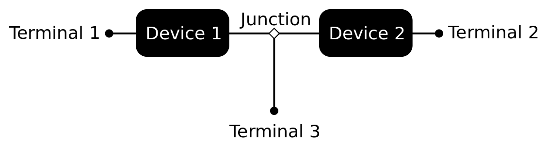
Figure 1: Schematic representation of the three-terminal system for measuring the voltage drop through the third terminal located between of two chaotic devices.

II.2 Voltage drop deviation $f$ in terms of scattering elements

Equation (2) is equivalent to the conductance but for three-terminal devices. Analogously to the conductance the problem of the voltage drop in electronic devices is reduced to a scattering problem through the quantity $f$. It is clear that $f$ contains all the information about the system by means of the transmission coefficients $T_{ij}$. Let us assume that the scattering properties of each device are known through their scattering matrices, $S_{1}$ for Device 1 and $S_{2}$ for Device 2. The general structure of these matrices depends on the symmetry properties of the problem, namely

$$S_{j}=\left(\begin{array}[]{cc}r_{j}J&t^{\prime}_{j}D_{j}\\ t_{j}D_{j}^{R}&r^{\prime}_{j}J\end{array}\right),\quad j=1,\,2,$$ (3)

where $r_{j}$ ($r^{\prime}_{j}$) and $t_{j}$ ($t^{\prime}_{j}$) are the reflection and transmission amplitudes for incidence from the left (right) of the Device $j$. Unitarity is the only requirement on $S_{j}$ in absence of any symmetry; this case is known as the Unitary symmetry and is labeled by $\beta=2$ in Dyson’s scheme. In addition, in the presence of time reversal invariance $S_{j}$ is unitary and symmetric, which corresponds to the Orthogonal symmetry and is labeled by $\beta=1$; for both cases $D_{j}=D_{j}^{R}=J=1$. Furthermore, in the presence of time-reversal invariance but no spin-rotation symmetry, the symmetry of the system is the Symplectic one, labeled by $\beta=4$, and $S_{j}$ becomes a $4\times 4$ self-dual matrix RMP69 in which case $J$ is the $2\times 2$ identity matrix, $J=\openone$, and $D_{j}^{R}$ is the dual matrix of the $2\times 2$ matrix $D_{j}$, defined by Karol

$$D_{j}^{R}=-ZD_{j}^{T}Z,$$ (4)

with $D_{j}^{T}$ the transposed matrix of $D_{j}$ and

$$Z=\left(\begin{array}[]{cc}0&-1\\ 1&0\end{array}\right).$$ (5)

The dependence of $T_{ij}$ on $S_{1}$ and $S_{2}$ can be obtained explicitly. The scattering matrix of the three-terminal symmetric configuration is given by Angel2014

$$\mathbf{S}=S_{PP}+S_{PQ}(S_{0}-S_{QQ})^{-1}S_{QP},$$ (6)

where $S_{0}$ is the scattering matrix of the junction that accounts for the coupling to the probe. In fact, $S_{0}$ can be obtained from the experiment Angel2018 ; Abdu2018 , it reads as

$$S_{0}=\frac{1}{3}\left(\begin{array}[]{ccc}-J&2J&2J\\ 2J&-J&2J\\ 2J&2J&-J\end{array}\right).$$ (7)

In Eq. (6) $S_{PP}$ represents the reflections to the terminals, $S_{QP}$ and $S_{PQ}$ represent the transmissions from the terminals to the inner part of the system and from the inner part to the terminals; $S_{QQ}$ represents the internal reflections and $(S_{0}-S_{QQ})^{-1}$ accounts for the multiple scattering between the Devices and the junction. Explicitly, they are

$$\begin{array}[]{cc}\vspace{0.5cm}S_{PP}=\left(\begin{array}[]{ccc}r_{1}J&0&0\\ 0&r^{\prime}_{2}J&0\\ 0&0&0\end{array}\right),&S_{PQ}=\left(\begin{array}[]{ccc}t^{\prime}_{1}D_{1}&0&0\\ 0&t_{2}D^{R}_{2}&0\\ 0&0&J\end{array}\right),\\ S_{QP}=\left(\begin{array}[]{ccc}t_{1}D^{R}_{1}&0&0\\ 0&t^{\prime}_{2}D_{2}&0\\ 0&0&J\end{array}\right),&S_{QQ}=\left(\begin{array}[]{ccc}r^{\prime}_{1}J&0&0\\ 0&r_{2}J&0\\ 0&0&0\end{array}\right).\end{array}$$ (8)

By substituting Eqs. (7) and (8) into Eq. (6), the scattering matrix elements $\mathbf{S}_{31}$ and $\mathbf{S}_{32}$ are obtained, from which $T_{ij}=|\mathbf{S}_{ij}|^{2}$ for $\beta=1,\,2$, while $T_{ij}=\frac{1}{2}\mathrm{tr}(\mathbf{S}_{ij}\mathbf{S}^{\dagger}_{ij})$ for $\beta=4$, and therefore Eq. (2) reduces to

$$f=\frac{|t_{1}|^{2}|1+r_{2}|^{2}-|t^{\prime}_{2}|^{2}|1+r^{\prime}_{1}|^{2}}{|t_{1}|^{2}|1+r_{2}|^{2}+|t^{\prime}_{2}|^{2}|1+r^{\prime}_{1}|^{2}}.$$ (9)

Note that $S_{31}$, $S_{32}$, and $f$ depend only on the elements of the individual scattering matrices that describe the devices.

III Chaotic scattering for the voltage drop deviation

Of particular interest are the transport properties through chaotic devices, quantum or classical. The disordered three-terminal system was previously considered in Ref. Godoy1992b . In any case the scattering quantities, like the transmission coefficients through each device, fluctuate with respect to a tuning parameter, like the energy of the incident particles in the quantum case or the frequency in the classical wave situation, or from sample to sample. Therefore, it is the distribution of $f$ what becomes more important rather than a particular value of $f$.

For a chaotic cavity, the statistical fluctuations of the scattering matrix are described by RMT. There, $S_{j}$ is uniformly distributed according to the invariant measure $\mathrm{d}\mu_{\beta}(S_{j})$ that defines the circular ensemble for the symmetry class $\beta$: the Circular Orthogonal Ensemble for $\beta=1$, the Circular Unitary Ensemble for $\beta=2$, and the Circular Symplectic Ensemble for $\beta=4$. Hence, the statistical distribution of $f$ can be calculated from the definition

$$P_{\beta}(f)=\int\delta\left(f-\frac{T_{31}-T_{32}}{T_{31}+T_{32}}\right)\mathrm{d}\mu_{\beta}(S_{1})\,\mathrm{d}\mu_{\beta}(S_{2}),$$ (10)

where $\delta$ is the Dirac delta function.

III.1 Statistical distribution of the voltage drop deviation $f$

A useful parameterization for scattering matrices is the polar form

$$S_{j}=\left[\begin{array}[]{cc}-\sqrt{1-\tau_{j}}\textnormal{e}^{\textnormal{i}(\phi_{j}+\phi^{\prime}_{j})}J&\sqrt{\tau_{j}}\textnormal{e}^{\textnormal{i}(\phi_{j}+\psi^{\prime}_{j})}D_{j}\\ \sqrt{\tau_{j}}\textnormal{e}^{\textnormal{i}(\psi_{j}+\phi^{\prime}_{j})}D_{j}^{R}&\sqrt{1-\tau_{j}}\textnormal{e}^{\textnormal{i}(\psi_{j}+\psi^{\prime}_{j})}J\end{array}\right],$$ (11)

where $0\leq\tau_{j}\leq 1$ and $\phi_{j}$, $\phi^{\prime}_{j}$, $\psi_{j}$, $\psi^{\prime}_{j}$ lie in the interval $[0,\,2\pi]$; $\phi_{j}=\phi^{\prime}_{j}$ and $\psi_{j}=\psi^{\prime}_{j}$ for $\beta=1,\,4$. Also, for $\beta=4$, $D_{j}$ can be parameterized as

$$D_{j}=U_{j}V_{j}^{R}.$$ (12)

where $U_{j}$ and $V_{j}$ are $2\times 2$ special unitary matrices and $V_{j}^{R}$ is the dual of $V_{j}$, as defined in Eq. (4).

For this parameterization, the normalized invariant measure of $S_{j}$ is given by

$$\mathrm{d}\mu_{\beta}(S_{j})=p_{\beta}(\tau_{j})\,\mathrm{d}\tau_{j}\,\frac{\mathrm{d}\phi_{j}}{2\pi}\,\frac{\mathrm{d}\psi_{j}}{2\pi}\times\left\{\begin{array}[]{lr}\vspace{0.1cm}1\,,&\quad\beta=1,\\ \vspace{0.1cm}\displaystyle{\frac{\mathrm{d}\phi^{\prime}_{j}}{2\pi}\,\frac{\mathrm{d}\psi^{\prime}_{j}}{2\pi},}&\beta=2\,,\\ \displaystyle{\mathrm{d}\mu(U_{j})\,\mathrm{d}\mu(V_{j})}\,,&\beta=4,\end{array}\right.$$ (13)

where

$$p_{\beta}(\tau_{j})=\frac{\beta}{2}\tau_{j}^{\beta/2-1},$$ (14)

$\mathrm{d}\mu(U_{j})$ and $\mathrm{d}\mu(V_{j})$ are the invariant measures of $U_{j}$ and $V_{j}$, respectively. As we will see in what follows, $f$ does not depend neither on $U_{j}$ nor $V_{j}$ such that we do not need to know explicitly the expressions for $\mathrm{d}\mu(U_{j})$ and $\mathrm{d}\mu(V_{j})$ .

In terms of the parameterization of Eq. (11) the voltage drop deviation, given in Eq. (9), can be written as

$$f=1+\frac{\tau_{1}\tau_{2}-2\tau_{2}-2\tau_{2}\sqrt{1-\tau_{1}}\cos{(\psi_{1}+\psi^{\prime}_{1}})}{\tau_{1}+\tau_{2}-\tau_{1}\tau_{2}-\tau_{1}\sqrt{1-\tau_{2}}\cos{(\phi_{2}+\phi^{\prime}_{2})}+\tau_{2}\sqrt{1-\tau_{1}}\cos{(\psi_{1}+\psi^{\prime}_{1}})}.$$ (15)

Since $f$ does not depend neither on $U_{j}$ nor $V_{j}$, the integration over $\mathrm{d}\mu(U_{j})$ and $\mathrm{d}\mu(V_{j})$ in Eq. (10) gives just 1 for $\beta=4$; except for variables $\tau_{1}$ and $\tau_{2}$, the resulting expression for $P_{\beta}(f)$ reduces to a one similar to that for $\beta=1$ in the remaining variables. The integration of $\mathrm{d}\phi_{1}/2\pi$, $\mathrm{d}\phi^{\prime}_{1}/2\pi$, $\mathrm{d}\psi_{2}/2\pi$, and $\mathrm{d}\psi^{\prime}_{2}/2\pi$ gives 1 for $\beta=2$. Therefore, once we perform the integration with respect to $\phi_{2}$ and $\phi_{2}^{\prime}$, making the appropriate change of variables for each symmetry class, and then with respect to the remaining phases $\psi_{1}$ and $\psi_{1}^{\prime}$, we arrive at

$$P_{\beta}(f)=\int_{0}^{1}\mathrm{d}\tau_{1}\int_{0}^{1}\mathrm{d}\tau_{2}\,p_{\beta}(\tau_{1})\,p_{\beta}(\tau_{2})\,p(f|\tau_{1},\tau_{2}),$$ (16)

where $p(f|\tau_{1},\tau_{2})$, which can be interpreted as the conditional probability distribution of $f$ given $\tau_{1}$ and $\tau_{2}$, is given by

$$\ p(f|\tau_{1},\tau_{1}) = \frac{1}{\pi^{2}\left(1-f^{2}\right)\sqrt{1-\tau_{1}}}\times$$

$$\int_{L}\frac{2-\tau_{1}+2\sqrt{1-\tau_{1}}\,x}{\sqrt{\left(\alpha_{+}-x\right)\left(x-\alpha_{-}\right)\left(1-x^{2}\right)}}\,\mathrm{d}x,$$

where $L\in(-1,1)\cap(\alpha_{-},\alpha_{+})$ with

$$\alpha_{\pm}=\frac{(\tau_{1}-\tau_{2})-(\tau_{1}+\tau_{2}-\tau_{1}\tau_{2})f\pm(1-f)\tau_{1}\sqrt{1-\tau_{2}}}{(1+f)\tau_{2}\sqrt{1-\tau_{1}}},$$ (18)

The integration in the domain $L$ is not a trivial problem because it depends on the variables $\tau_{1}$, $\tau_{2}$, and $f$ through $\alpha_{\pm}$ in a complicated way, but we can give a further step in the integration by looking for the limits of integration once the value of $f$ is fixed (see Appendix A for details). The integral over $x$ in Eq. (III.1) can be expressed in terms of complete elliptic integrals. The result for $P_{\beta}(f)$ can be expressed as

$$P_{\beta}(f) = \frac{1}{\pi^{2}(1-f^{2})}\times$$

$$\left[\int_{0}^{1}\mathrm{d}\tau_{1}\frac{p_{\beta}(\tau_{1})}{\sqrt{1-\tau_{1}}}\int_{0}^{u(\tau_{1})}\mathrm{d}\tau_{2}\,p_{\beta}(\tau_{2})\,I_{-1}^{1}(f;\tau_{1},\tau_{2})\right.$$

$$+ \int_{0}^{1}\mathrm{d}\tau_{2}\,p_{\beta}(\tau_{2})\,\int_{0}^{w(\tau_{2})}\mathrm{d}\tau_{1}\frac{p_{\beta}(\tau_{1})}{\sqrt{1-\tau_{1}}}\,I_{\alpha_{-}}^{\alpha_{+}}(f;\tau_{1},\tau_{2})$$

$$+ H(f)\,H(1-f)\int_{0}^{1}\mathrm{d}\tau_{1}\frac{p_{\beta}(\tau_{1})}{\sqrt{1-\tau_{1}}}\times$$

$$\int_{u(\tau_{1})}^{v(\tau_{1})}\,\mathrm{d}\tau_{2}\,p_{\beta}(\tau_{2})\,I_{-1}^{\alpha_{+}}(f;\tau_{1},\tau_{2})$$

$$+ \left.H(-f)\,H(f+1)\int_{0}^{1}\mathrm{d}\tau_{1}\frac{p_{\beta}(\tau_{1})}{\sqrt{1-\tau_{1}}}\right.\times$$

$$\left.\int_{u(\tau_{1})}^{v(\tau_{1})}\mathrm{d}\tau_{2}\,p_{\beta}(\tau_{2})\,I_{\alpha_{-}}^{1}(f;\tau_{1},\tau_{2})\right],$$

where $H(x)$ is the Heaviside step function and the limits are

$$u(\tau_{1}) = \frac{r(2s_{-}-r)}{s_{-}^{2}},\quad v(\tau_{1})=\frac{r(2s_{+}-r)}{s_{+}^{2}},\quad$$ (20)

$$\mathrm{and}\quad w(\tau_{2})=\frac{r^{\prime}(2s^{\prime}-r^{\prime})}{{s^{\prime}}^{2}},$$

where $r^{\prime}=r(\tau_{1}\to\tau_{2})$ and $s^{\prime}=s_{-}(\tau_{1}\to\tau_{2})$ with

$$r(\tau_{1}) = (1-f)\tau_{1}\quad\mbox{and}\quad$$

$$s_{\pm}(\tau_{1}) = 1+(1-\tau_{1})f\pm(1+f)\sqrt{1-\tau_{1}}.$$ (21)

In Eq. (III.1),

$$I_{-1}^{1}(f;\tau_{1},\tau_{2})=\frac{2}{\sqrt{(\alpha_{+}+1)(1-\alpha_{-})}}$$

$$\times [(A+B\alpha_{-})K(k_{1})-(1+\alpha_{-})B\,\Pi(r_{1}^{2},k_{1})],$$

$$I_{\alpha_{-}}^{\alpha_{+}}(f;\tau_{1},\tau_{2})=\frac{2}{\sqrt{(\alpha_{+}+1)(1-\alpha_{-})}}$$

$$\times [(A-B)K(k_{1})+(1+\alpha_{-})B\,\Pi({r^{\prime}_{1}}^{2},k_{1})],$$

$$I_{-1}^{\alpha_{+}}(f;\tau_{1},\tau_{2})=\frac{\sqrt{2}}{\sqrt{\alpha_{+}-\alpha_{-}}}$$

$$\times [(A+B\alpha_{-})K(k_{2})-(1+\alpha_{-})B\,\Pi({r^{\prime}_{2}}^{2},k_{2})],$$

and

$$I_{\alpha_{-}}^{1}(f;\tau_{1},\tau_{2})=\frac{\sqrt{2}}{\sqrt{\alpha_{+}-\alpha_{-}}}$$

$$\times [(A-B)K(k_{2})+(1+\alpha_{-})B\,\Pi({r_{2}}^{2},k_{2})],$$

where $A=2-\tau_{1}$ and $B=2\sqrt{1-\tau_{1}}$; $K(k)$ and $\Pi(r^{2},k)$ are complete elliptic integrals of the first and third kind, respectively, and

$$k_{1}^{2} = \frac{2(\alpha_{+}-\alpha_{-})}{(\alpha_{+}+1)(1-\alpha_{-})},\quad r_{1}^{2}=\frac{2}{1-\alpha_{-}},$$ (26)

$$\quad\mbox{and}\quad{r^{\prime}_{1}}^{2}=\frac{\alpha_{+}-\alpha_{-}}{\alpha_{+}+1};$$

$$k_{2}^{2}=\frac{1}{k_{1}^{2}},\quad r_{2}^{2}=\frac{1}{r_{1}^{2}},\quad\mbox{and}\quad{r^{\prime}_{2}}^{2}=\frac{1}{{r^{\prime}_{1}}^{2}}.$$ (27)

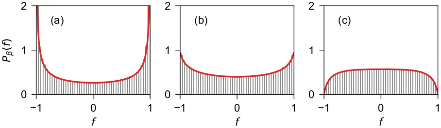
Figure 2: Comparison between the analytical results (continuous lines) with random matrix simulations (histograms) for $P_{\beta}(f)$: (a) $\beta=1$, (b) $\beta=2$, and (c) $\beta=4$.

The remaining integrals with respect to $\tau_{1}$ and $\tau_{2}$ can be performed numerically. In order to verify our results, in Fig. 2 we compare them with the statistical distributions obtained from numerical simulations using Eqs. (11)-(15). An excellent agreement is observed.

We can observe in Fig. 2 that the distribution of $f$ is symmetric with respect to $f=0$. Moreover, it diverges at $f=\pm 1$ for $\beta=1$, while it shows finite peaks at $f=\pm 1$ for $\beta=2$, which is a clear effect of the weak localization. For $\beta=4$ the distribution becomes zero at $f=\pm 1$ due to the antilocalization phenomenon. The differences found in the $P_{\beta}(f)$ between the symmetry classes are important signatures of the chaotic setup we consider here, since in the equivalent disordered configuration no differences were found Godoy1992b .

IV Experimental realizations with microwave graphs

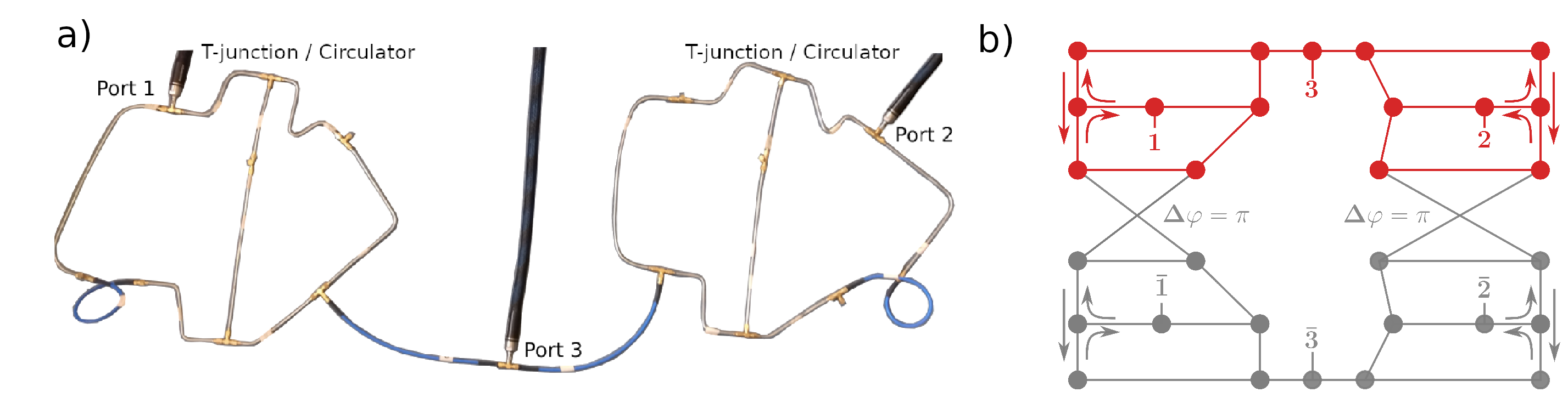
Figure 3: (a) Photograph of the three-port experimental setup for the case of time-reversal symmetry ($\beta=1$). For the realization of a break of time-reversal symmetry ($\beta=2$) one T junction in each of the subgraphs is replaced by a circulator. Both subgraphs are geometrically different but have the same total length, i. e., the mean level density is the same. (b) Sketch of the graph for $\beta=1$ (GOE) and $\beta=2$ (GUE), where for $\beta=1$ the circulators are replaced by ordinary T junctions (red). For a realization of $\beta=4$ (GSE) each GUE subgraph is complemented by another geometrically identical one but with an opposite sense of rotation of the circulators (grey). The two respective copies are connected by pairs of bonds with length differences corresponding to a phase difference of $\pi$ for the propagating waves (see Ref. Abdu2016 for details, where also a photograph of a single GSE graph can be found).

Since the voltage drop deviation depends only on the scattering properties of the devices, it can be emulated in classical wave systems, in particular experiments with microwave graphs can be performed. Figure 3(a) shows a photograph of the experimental set-up for the case of time-reversal invariance ($\beta=1$). The devices consist of chaotic microwave networks formed by coaxial semirigid cables (Huber & Suhner EZ-141) with SMA connectors, coupled by T junctions at the nodes. One microwave port attached to the left subgraph acts as the input, another one on the right as the output, and a third port attached to the connecting cable between the two subgraphs as the probe. To realize a break of time-reversal invariance ($\beta=2$), in each of the two subgraphs one of the T junctions is replaced by a circulator (Aerotek I70-1FFF) with an operating frequency range from 6 to 12 GHz. A circulator introduces directionality, waves entering via port 1 leave via port 2. The transmission intensities $T_{31}$ and $T_{32}$ were measured by an Agilent 8720ES vector network analyzer (VNA). The $\beta=1$ case has been additionally realized in a billiard setup. Details are presented in Appendix B.

For the realization of the $\beta=4$ (GSE) case two GSE graphs are needed. Since each GSE graph is composed by two GUE subgraphs, representing the spin-up and spin-down components Abdu2016 , we need a total of four subgraphs. Figure 3(b) shows a sketch of the three-terminal GSE graph used to measure the scattering matrix. An essential ingredient of the setup are two pairs of bonds with length differences $\Delta l$ corresponding to phase differences of $\Delta\varphi=\pi$ for the propagating waves. In the experiment we took spectra for fixed $\Delta l$ and converted them into spectra for fixed $\Delta\varphi$ using $\Delta\varphi=k\Delta l$, where $k$ is the wavenumber. Details can be found in Ref. Abdu2016 . The ports now appear in pairs $1,\bar{1},2,\bar{2},3,\bar{3}$, and the scattering matrix elements turn into $2\times 2$ matrices

$$\mathbf{S}_{ij}=\left(\begin{array}[]{cc}S_{ij}&S_{i\bar{j}}\\ S_{\bar{i}j}&S_{\bar{i}\bar{j}}\end{array}\right).$$ (30)

In the spirit of the spin analogy, $S_{ij}$ and $S_{i\bar{j}}$ correspond to transmissions without and with spin-flip, respectively. $\mathbf{S}_{ij}$ may be written in terms of quaternions as $\mathbf{S}_{ij}=S^{0}_{ij}\openone+\mathrm{i}S^{x}_{ij}\sigma_{x}+\mathrm{i}S^{y}_{ij}\sigma_{y}+\mathrm{i}S^{z}_{ij}\sigma_{z}$, where for a symplectic symmetry all coefficients $S^{0}_{ij}$, $S^{x}_{ij}$, etc. are real numbers and $\sigma_{j}$ is the corresponding Pali matrix $j$. As a consequence $\mathbf{S}_{ij}\mathbf{S}_{ij}^{\dagger}$ is a multiple of the unit matrix which allows for a simple check of the quality of the realization of the setup with symplectic symmetry. In our experiments $\mathbf{S}_{31}$ and $\mathbf{S}_{32}$ were found to be quaternion real within an error of $2.19\%$ and $1.93\%$, respectively. The mentioned multiple is nothing but the transmission coefficient, hence $T_{31}=\frac{1}{2}\mathrm{tr}(\mathbf{S}_{31}\mathbf{S}_{31}^{\dagger})$ and $T_{32}=\frac{1}{2}\mathrm{tr}(\mathbf{S}_{32}\mathbf{S}_{32}^{\dagger})$.

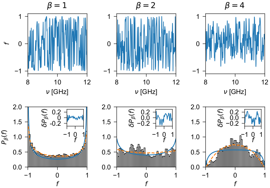
Figure 4: (Color online) Experimental voltage drop deviation $f$ as a function of frequency is shown in the upper panels for the three symmetry classes. Their corresponding statistical distribution are shown as histograms. The continuous (blue) lines in the lower panels correspond to the theoretical result shown in Fig 2, while the dashed (orange) lines are the RMT simulations which take into account the dissipation and imperfect coupling: $\beta=1$ (left), $\beta=2$ (middle), and $\beta=4$ (right). For comparison purposes, in the insets in the lower panels we show the difference between the numerical and the experimental distribution $\delta P_{\beta}(f)=P_{\beta}(f)_{\mathrm{num}}-P_{\beta}(f)_{\mathrm{expt}}$. For the statistical analysis we used an ensemble of $5\times 10^{4}$ realizations.

The experimental distribution of $f$ is shown in Fig. 4 as histograms for the three symmetry classes $\beta$, where it is compared with the theoretical result given by Eq. (III.1). As can be observed there is a qualitatively good agreement for all $\beta$. Despite the fact that there is a quantitative difference between theory and experiment, which is due to the phenomena of dissipation and imperfect coupling between the graphs and ports, this difference is not so large. In Fig. 4 we also show the corrected distribution obtained from RMT simulations, using the Heidelberg approach (see below), once these two phenomena, dissipation and imperfect coupling, are taken into account.

The dissipation and imperfect coupling can be quantified by two parameters: $T_{1}$ for the coupling strength and $\gamma$ for the dissipation. The coupling between the graphs and ports $T_{1}$ is extracted from the experimental data as $T_{1}=1-|\langle S_{11}\rangle|^{2}$, where $\langle S_{11}\rangle$ is the average (with respect to the frequency) of the scattering matrix element 11. Here we obtained $T_{1}=0.99$ for $\beta=1$, $T_{1}=0.99$ for $\beta=2$, and $T_{1}=0.953$ for $\beta=4$. As can be seen the coupling strength is almost 1, which means that the coupling between graphs and ports, although not perfect, can be considered as very good. The effect of dissipation is clearly observed in the experimental transmission intensities $T_{31}$ and $T_{32}$. Their fluctuations as a function of the frequency are shown in Fig. 5, where we observe that they do not reach the value 1. The dissipation parameter $\gamma$ can be quantified by fitting the autocorrelation function $C_{11}(t)$ of the 11 element of the scattering matrix Schafer2003 ; Angel2018 ; Fyodorov2005b

$$\frac{C_{11}(t)}{T_{1}^{2}}=\left\{\begin{array}[]{ll}\vspace{0.1cm}\left[\displaystyle{\frac{3}{(1+2T_{1}t)^{3}}-\frac{b_{1,2}(t)}{(1+T_{1}t)^{4}}}\right]\mathrm{e}^{-\gamma t}&\mbox{for}\,\,\beta=1,\\ \vspace{0.1cm}\left[\displaystyle{\frac{2}{(1+T_{1}t)^{4}}-\frac{2^{6}b_{2,2}(t)}{(2+T_{1}t)^{6}}}\right]\mathrm{e}^{-\gamma t}&\mbox{for}\,\,\beta=2,\\ \left[\displaystyle{\frac{6}{(1+T_{1}t)^{6}}-\frac{2^{12}b_{4,2}(t)}{(2+T_{1}t)^{10}}}\right]\mathrm{e}^{-2\gamma t}&\mbox{for}\,\,\beta=4,\end{array}\right.$$ (31)

where $b_{\beta,2}(t)$ is the two-level form factor Guhr1998 and $T_{1}$, $\gamma$, and $t$ are given in dimensionless units. The best fit achieved for $C_{11}(t)$, for $t<1$, is shown in Fig. 5 for all symmetry classes, for which we obtain $\gamma=2.6$ for $\beta=1$, $\gamma=2.0$ for $\beta=2$, and $\gamma=1.8$ for $\beta=4$.

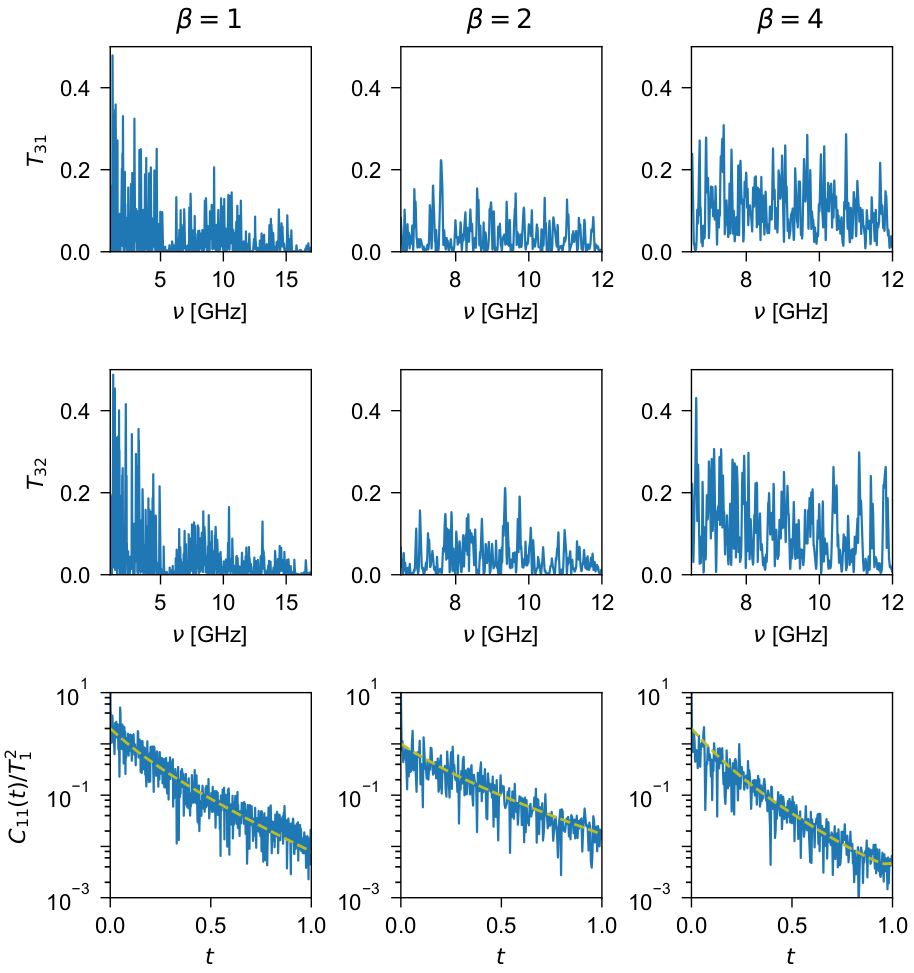
Figure 5: Experimental transmission intensities $T_{31}$ and $T_{32}$ as a function of frequency are shown in upper and middle panels for the three symmetry classes. The lower panels show the autocorrelation function: the fluctuations are the experimental measurements and the dashed lines are the best fits of Eq. (31) to the data for $t<1$.

Once these parameters are determined, RMT simulations can be performed for the scattering matrix of each graph, assumed as quantum systems. In the Heidelberg approach the scattering matrix of a graph can be generated as Brouwer1997

$$S_{g}=1-2\pi\mathrm{i}W^{\dagger}\frac{1}{E-\mathcal{H}+\mathrm{i}\pi WW^{\dagger}}W,$$ (32)

where $E$ represents the energy of the incoming wave and $W$ is the matrix that couples the open modes in the ports to the internal modes of the system. $\mathcal{H}$ is an effective Hamiltonian that includes the dissipation $\gamma$, $\mathcal{H_{\mu\nu}}=H_{\mu\nu}-\mathrm{i}\delta_{\mu\nu}\gamma\Delta/4\pi$, with $\Delta$ the mean level spacing. The imperfect coupling can be modeled by adding identical barriers, with transmission intensity $T_{1}$, between the graph 1 and port 1, between the graphs and the T junction, and between graph 2 and port 2. The numerical simulations of the three-terminal system, with the obtained values of $T_{1}$ and $\gamma$, lead us to the result shown in Fig. 4 for the distribution of $f$; see the orange dashed lines in the lower panels. As can be observed, the agreement is very good.

V Conclusions

A three-terminal symmetrical system consisting of two microwave graphs was used to measure indirectly the voltage drop between the graphs. One port was used as an input, a second port as an exit, and a third port as a probe. The fluctuations of the quantity $f$, that accounts for the deviation from the mean value of the potentials, are explained qualitatively by an ideal result obtained from the scattering approach of random matrix theory for the three Dyson’s symmetry classes. We found that the distribution of $f$ is symmetric with respect to zero, whose shape is quite similar to the one obtained in the disordered case, in the insulating regime, but with an important difference which is the effect of weak localization and antilocalization phenomena not found in the disordered case. A more accurate description is obtained when dissipation and imperfect coupling between the ports and graphs are taken into account.

Appendix A Limits of integration in Eq. (III.1)

The integration with respect to $x\in(-1,1)$ in Eq. (III.1) should be performed in the interval $L$, which is the intersection of the intervals $(-1,1)$ and $(\alpha_{-},\alpha_{+})$. Since $\alpha_{+}$ and $\alpha_{-}$ depend on the values of $\tau_{1}$, $\tau_{2}$, and $f$, the values of $\tau_{1}$ and $\tau_{2}$ may be affected by that intersection for fixed $f$. This leads to integrals of the form

$$I_{a}^{b}(f,\tau_{1},\tau_{2})=\int_{a}^{b}\frac{(A+Bx)dx}{\sqrt{(\alpha_{+}-x)(x-\alpha_{-})(1+x)(1-x)}},$$ (33)

which gives rise to complete elliptic integrals of the first and third kind.

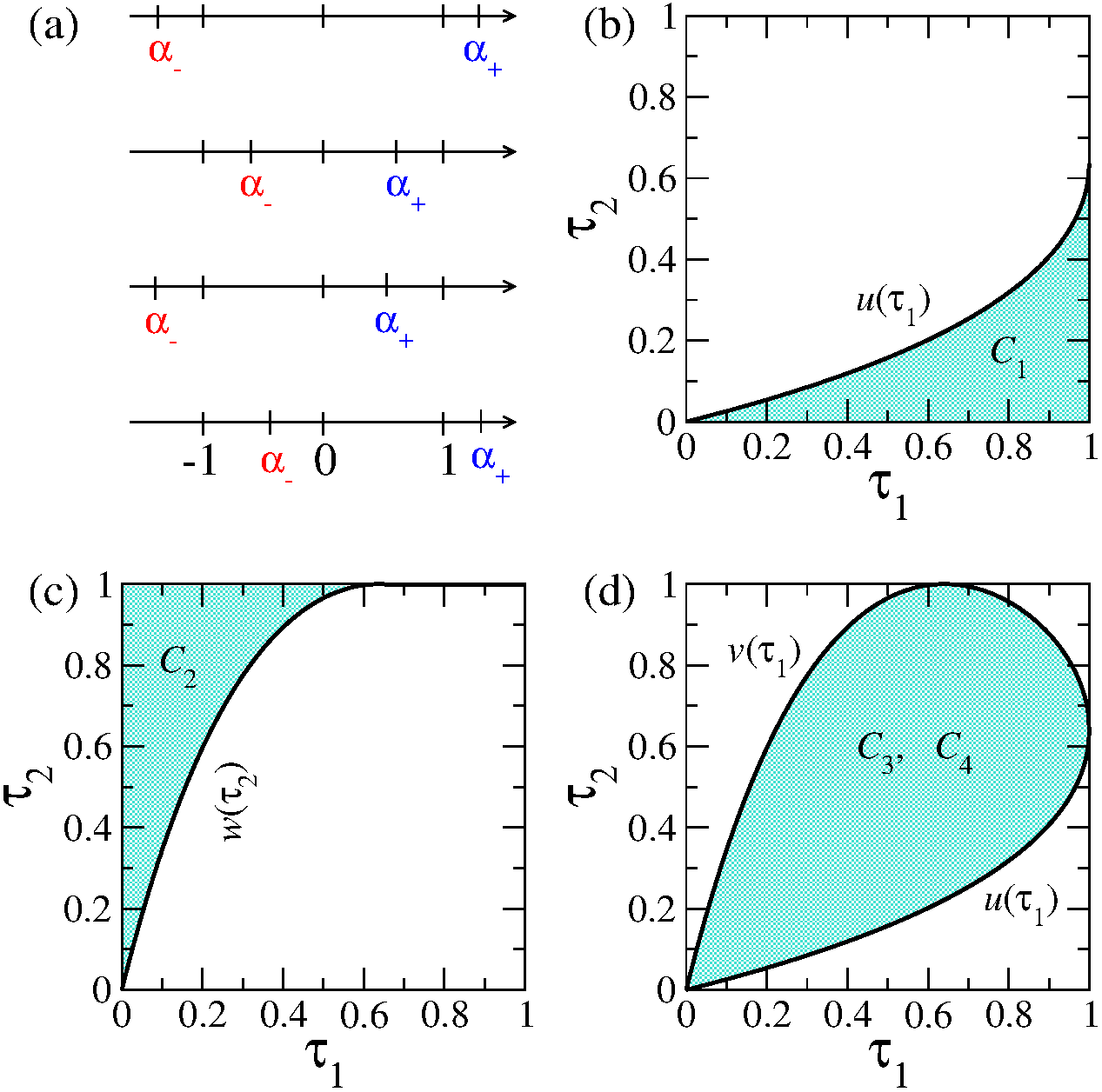
Figure 6: (a) Intervals of integration for $x$ which imply restrictions on $\tau_{1}$ and $\tau_{2}$ (shaded regions): for $|f|=0.6$ (b) $\tau_{2}\in(0,u(\tau_{1}))$ with $\tau_{1}\in(0,1)$; (c) $\tau_{1}\in(0,w(\tau_{2}))$ with $\tau_{2}\in(0,1)$; (d) $\tau_{2}\in(u(\tau_{1}),v(\tau_{1}))$ for $f>0$ and $\tau_{2}\in(v(\tau_{1}),u(\tau_{1}))$ for $f<0$, with $\tau_{1}\in(0,1)$. The functions $u(\tau)$, $v(\tau)$, and $w(\tau)$ are defined in Eq. (20).

Four conditions arise, as illustrated in Fig. 6(a). Restrictions on $\tau_{1}$ and $\tau_{2}$ are obtained for a fixed value of $f$. These restrictions lead to the several regions in the plane $\tau_{1}\tau_{2}$, as can be seen in Fig. 6.

Condition $C_{1}$

$\alpha_{-}\leq-1$ and $1\leq\alpha_{+}$. Under these conditions $x$ runs over its full domain, $x\in(-1,1)$. Restriction on $\tau_{2}$ for a fixed value of $f$ is obtained from these two conditions. The first condition, $\alpha_{-}\leq-1$, leads to $\tau_{2}\geq 0$ while the second condition, $1\leq\alpha_{+}$, restricts $\tau_{2}$ to be smaller than $u(\tau_{1})$, where $u(\tau_{1})$ is given in equation of (20). Therefore, $\tau_{2}\in(0,u(\tau_{1}))$ with $\tau_{1}\in(0,1)$.

Condition $C_{2}$

$-1\leq\alpha_{-}\leq\alpha_{+}\leq 1$. For this condition $x\in(\alpha_{-},\alpha_{+})$. Here, it is more convenient to see the restriction on $\tau_{1}$ for which we obtain that $\tau_{1}\in(0,w(\tau_{2}))$, where $w(\tau_{2})$ is given by the third equation in (20), for $\tau_{2}\in(0,1)$.

Condition $C_{3}$

$\alpha_{-}\leq-1$ and $-1\leq\alpha_{+}\leq 1$. The integration over $x$ is defined in the interval $(-1,\alpha_{+})$. The first part of the condition is the same as that for Condition $C_{1}$, which restricts to $\tau_{2}\geq 0$. The second condition has two parts, a first one is $\alpha_{+}\leq 1$ whose result is similar to the corresponding second part in Condition $C_{1}$, but the inequality in opposite sense; hence, $\tau_{2}\geq u(\tau_{1})$. In a similar manner, the second part $\alpha_{+}\geq-1$ leads to $\tau_{2}\leq v(\tau_{1})$ for $f>0$, which is given by the second equation in (20). Therefore, $\tau_{2}\in(u(\tau_{1}),v(\tau_{1}))$ with $\tau_{1}\in(0,1)$ and $f>0$.

Condition $C_{4}$

$-1\leq\alpha_{-}\leq 1$ and $1\leq\alpha_{+}$. The integration over $x$ is defined in the interval $(\alpha_{-},1)$. The second part of the condition is the same as that for Condition $C_{1}$ which restricts to $\tau_{2}\in(0,u(\tau_{1}))$ if $f$ is positive. The first condition has two parts, the first one, $\alpha_{-}\leq 1$ leads to the same restriction to $\tau_{2}$. The second part gives $\tau_{2}\in(v(\tau_{1}),1)$ for $f>0$. This result is equivalent to $\tau_{2}\in(u(\tau_{1}),v(\tau_{1}))$ for $f<0$.

To apply these conditions to the integral of Eq. (33) we use the equations 254.00, 254.10, 336.01, 336.60, and 340.04 of Ref. ByrdHandbook , then we integrate with respect to $\tau_{1}$ and $\tau_{2}$, and finally we arrive at Eq. (III.1).

Appendix B Three-port microwave billiard experiment

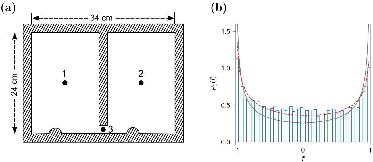
Figure 7: (a) Sketch of the three-port microwave billiard in the presence of $\beta=1$ symmetry. The ports are labeled as 1, 2, and 3, where port 3 is used as a probe. The experimental transmission intensities $T_{31}$ and $T_{32}$ are measured between ports 1 and 3, and between ports 2 and 3, respectively. (b) Distribution $P_{1}(f)$: the continuous (black) line corresponds to the theoretical result shown in Fig. 2, the dashed (red) line is the RMT simulation which takes into account dissipation and imperfect coupling, while the histogram corresponds to the experimental result.

For the $\beta=1$ case, in addition to the microwave graph experiments an experiment in a billiard setup has been performed. A sketch is shown in Fig. 7(a). The billiard is constructed on an aluminum plate with two sub-billiards of the same shape separated by a central bar. The mirror symmetry is broken by two semicircular obstacles, attached to the bottom boundary. The ports are labeled as 1, 2, and 3, where port 3 is used as a probe. The experimental transmission intensities $T_{31}$ and $T_{32}$ have been measured between port 1 and port 3, and between port 2 and port 3, respectively, for frequencies from 1 to 17 GHz. With a distance of $d=8$ mm between top and bottom plate the billiard is quasi-two-dimensional in the whole frequency range.

In panel (b) of Fig. 7 we show as histograms the experimental distribution of $P_{1}(f)$ obtained from the graph (black) and the billiard (blue) setting. The analytical result is shown in the continuous (black) line, while the RMT simulation, which take into account the dissipation and imperfect coupling, is shown in (red) dashed line. Again, a good agreement between experiment and theory is found for $P_{1}(f)$.

References

- (1) Y. V. Fyodorov, T. Kottos, H.-J. Stöckmann, Trends in quantum chaotic scattering, J. Phys. A: Math. Gen. 38 (2005) Preface.
- (2) H. Schanze, E. R. P. Alves, C. H. Lewenkopf, and H.-J. Stöckmann, Phys. Rev. E 64, 065201(R) (2001).
- (3) H. Schanze, H.-J. Stöckmann, M. Martínez-Mares, and C. H. Lewenkopf, Phys. Rev. E 71, 016223 (2005).
- (4) R. Schäfer, T. Gorin, T. H. Seligman, and H.-J. Stöckmann, J. Phys. A: Math. Gen. 36, 3289 (2003).
- (5) U. Kuhl, M. Martínez-Mares, R. A. Méndez-Sánchez, and H.-J. Stöckmann, Phys. Rev. Lett. 94, 144101 (2005).
- (6) M. Büttiker, IBM J. Res. Develop. 32, 317 (1988).
- (7) K. Schwab, E. A. H. J. M. Worlock, and M. L. Roukes, Nature 404, 974 (2000).
- (8) M. Büttiker, Y. Imry, and M. Y. Azbel, Phys. Rev. A 30, 1982 (1984).
- (9) P. W. Brouwer and C. W. J. Beenakker, Phys. Rev. B 55, 4695 (1997).
- (10) M. W. Keller, A. Mittal, J. W. Sleight, R. G. Wheeler, D. E. Prober, R. N. Sacks, and H. Shtrikmann, Phys. Rev. B 53, R1693 (1996).
- (11) C. M. Marcus, A. J. Rimberg, R. M. Westervelt, P. F. Hopkins, and A. C. Gossard, Phys. Rev. Lett. 69, 506 (1992) .
- (12) I. H. Chan, R. M. Clarke, C. M. Marcus, K. Campman, and A. C. Gossard, Phys. Rev. Lett. 74, 3876 (1995).
- (13) M. Martínez-Mares, Phys. Rev. E 72, 036202 (2005).
- (14) E. Flores-Olmedo, A. M. Martínez-Argüello, M. Martínez-Mares, G. Báez, J. A. Franco-Villafañe, and R. A. Méndez-Sánchez, Sci. Rep. 6, 25157 (2016).
- (15) M. Büttiker, Four-terminal phase-coherent conductance, Phys. Rev. Lett. 57, 1761 (1986).
- (16) V. A. Gopar, M. Martínez, and P. A. Mello, Phys. Rev. B 50, 2502 (1994).
- (17) L. Arrachea, C. Naón, and M. Salvay, Phys. Rev. B 77, 233105 (2008).
- (18) C. Texier and G. Montambaux, Physica E 82, 272 (2016).
- (19) F. Foieri, L. Arrachea, and M. J. Sánchez, Phys. Rev. B 79, 085430 (2009).
- (20) J. L. D’Amato and H. M. Pastawski, Phys. Rev. B 41, 7411 (1990).
- (21) C. J. Cattena, L. J. Fernández-Alcázar, R. A. Bustos-Marún, D. Nozaki, and H. M. Pastawski, J. Phys.: Condens. Matter 26, 345304 (2014).
- (22) A. M. Song, A. Lorke, A. Kriele, J. P. Kotthaus, W. Wegscheider, and M. Bichler, Phys. Rev. Lett. 80, 3831 (1998).
- (23) B. Gao, Y. F. Chen, M. S. Fuhrer, D. C. Glattli, and A. Bachtold, Phys. Rev. Lett. 95, 196802 (2005).
- (24) A. M. Martínez-Argüello, A. Rehemanjiang, M. Martínez-Mares, J. A. Méndez-Bermúdez, H.-J. Stöckmann, and U. Kuhl, Phys. Rev. B 98, 075311 (2018).
- (25) A. M. Martínez-Argüello, J. A. Méndez-Bermúdez, and M. Martínez-Mares, Phys. Rev. E 99, 062202 (2019).
- (26) S. Godoy and P. A. Mello, EPL 17, 243 (1992).
- (27) S. Godoy and P. A. Mello, Phys. Rev. B 46, 2346 (1992).
- (28) A. M. Martínez-Argüello, E. Castaño, and M. Martínez-Mares, Random matrix study for a three-terminal chaotic device, in Special Topics on Transport Theory: Electrons, Waves, and Diffusion in Confined Systems, AIP Conf. Proc. No. 1579 (AIP, Melville, NY , 2014), p. 46.
- (29) C. W. J. Beenakker, Rev. Mod. Phys. 69, 731 (1997).
- (30) K. Życzkowski, Random Matrices of Circular Symplectic Ensemble in Chaos–The Interplay Between Stochastic and Deterministic Behaviour, Lecture Notes in Physics, vol 457, edited by P. Garbaczewski, M. Wolf, and A. Weron (Springer, Berlin, Heidelberg, 1995).
- (31) A. Rehemanjiang, M. Richter, U. Kuhl, and H.-J. Stöckmann, Phys. Rev. E 97, 022204 (2018).
- (32) A. Rehemanjiang, M. Allgaier, C. H. Joyner, S. Müller, M. Sieber, U. Kuhl, and H.-J. Stöckmann, Phys. Rev. Lett. 117, 064101 (2016).
- (33) Y. V. Fyodorov, D. V. Savin, and H.-J. Sommers, J. Phys. A: Math. Gen. 38, 10731 (2005).
- (34) T. Guhr, A. Müller-Groeling, and H. A. Weidenmüller, Phys. Rep. 299, 189 (1998).
- (35) P. F. Byrd and M. D. Friedman, Handbook of Elliptic Integrals for Engineers and Physicists, Springer-Verlag Berlin Heidelberg GMBH, Berlin, Heidelberg, 1954.