Helical turbulent nonlinear dynamo at large magnetic Reynolds numbers

Abstract

The excitation and further sustenance of large-scale magnetic fields in rotating astrophysical systems, including planets, stars and galaxies, is generally thought to involve a fluid magnetic dynamo effect driven by helical magnetohydrodynamic turbulence. While this scenario is appealing on general grounds, it however currently remains largely unconstrained, notably because a fundamental understanding of the nonlinear asymptotic behaviour of large-scale fluid magnetism in the astrophysically-relevant but treacherous regime of large magnetic Reynolds number $Rm$ is still lacking. We explore this problem using local high-resolution simulations of turbulent magnetohydrodynamics driven by an inhomogeneous helical forcing generating a sinusoidal profile of kinetic helicity, mimicking the hemispheric distribution of kinetic helicity in rotating turbulent fluid bodies. We identify a transition at large $Rm$ to a nonlinear state, followed up to $Rm\simeq 3\times 10^{3}$, consisting of strong, saturated small-scale magnetohydrodynamic turbulence and a weaker, travelling coherent large-scale field oscillation. This state is characterized by an asymptotically small resistive dissipation of magnetic helicity, by its spatial redistribution across the equator through turbulent fluxes driven by the hemispheric distribution of kinetic helicity, and by the tentative presence in the tangled dynamical magnetic field of plasmoids typical of reconnection at large $Rm$.

Introduction.

Magnetic fields pervading astrophysical fluid systems such as stars and galaxies are commonly thought to be excited and further sustained by a variety of self-amplifying magnetohydrodynamic (MHD) dynamo effects converting kinetic energy of turbulent flows of electrically-conducting fluid into magnetic energy [1, 2, 3, 4, 5, 6, 7]. In order to sustain large-scale magnetic fields via a turbulent dynamo, however, some underlying system-scale symmetry-breaking is generically required. Typically, this is provided in astrophysical systems by large-scale rotation and/or shear. In particular, by breaking the parity/mirror invariance of an otherwise isotropic, homogeneous turbulence, rotation makes the turbulence helical. This creates the conditions for statistical dynamo effects that can in principle amplify large-scale magnetic fields exponentially on a rotation timescale [8, 9, 10, 11]. The most well-known, the $\alpha$ effect [12], is generally considered a key ingredient of magnetic-field generation in the Sun.

While a helical turbulent dynamo provides an appealing phenomenological explanation for the large-scale magnetism of rotating astrophysical bodies, there remain major open questions regarding its actual viability and efficiency in the regime of large magnetic Reynolds numbers $Rm$ and comparable flow turnover times and correlation times, an astrophysically-relevant non-perturbative limit for which no analytical theory is available [13, 14] ($Rm=UL/\eta$ is larger than $10^{6}$ in the Sun, and $10^{20}$ in galaxies ; $U$ denotes a typical velocity field amplitude, $L$ is the typical scale of the turbulence, and $\eta$ is the magnetic diffusivity). Numerical studies have shown that large-scale exponential dynamo growth driven by helical turbulence, such as rotating convection, is possible at mild $Rm<O(100)$ ([15, 16], see also [5, 6, 17] for reviews in various astrophysical contexts), however this regime is still far from asymptotic in practice.

First of all, a distinct small-scale “fluctuation” dynamo mechanism is activated beyond $Rm=O(100)$, that amplifies magnetic fields on fast time and spatial scales comparable to the flow turnover scales [18, 19, 20, 21, 22]. This dynamo populates a large-$Rm$ turbulent MHD fluid with dynamical small-scale fields affecting the structure of the flow much faster than the helical dynamo can grow a large-scale field [23, 24, 25]. Besides, independently of a small-scale dynamo, turbulent tangling of a growing large-scale field produces dynamical magnetic fluctuations at increasingly smaller-scales as $Rm$ increases (typically $\propto Rm^{-1/2}$), resulting in small-scale dynamical feedback on the flow well before the large-scale field has itself saturated [26]. In the case of homogeneous helical turbulence producing an $\alpha$ effect, this problem takes a particular pathological form: the large-scale field does ultimately reach super-equipartition levels, but it can only do so on a long, system-scale resistive time, a consequence of a resistive bottleneck in the dissipation of small-scale magnetic twists also responsible for the dynamical reduction of the $\alpha$ effect [27, 16, 28, 29]. This is usually referred to as the catastrophic $\alpha$-quenching problem. Finally, the resistive-scale dynamics of saturated MHD dynamos may undergo a fast-reconnection transition at $Rm=O(S_{c})$, where $S_{c}=O(10^{4})$ is the critical value of the Lundquist number $S=LV_{A}/\eta$ at which MHD reconnection becomes fast [30, 31, 32] (assuming an Alfvén speed $V_{A}\sim U$ in the saturated regime). Its implications for the dynamics of helical fields, such as produced by the $\alpha$ effect, have so far barely been touched on [33, 34, 35, 36, 7, 37, 38].

We aim to further explore the nonlinear helical dynamo problem at large $Rm$. A long-envisioned possible solution to catastrophic quenching is via removal or spatial redistribution of small-scale magnetic helicity by helicity fluxes [39, 40, 41, 42, 43, 44, 45, 46, 47]. The most studied case [48, 49, 50] involves expulsion of magnetic helicity through system boundary winds. Simulations up to $Rm\simeq 10^{3}$ suggest that a regime with subdominant resistive effects is achieved at large $Rm$ [50]. Alternatively, a similar state may be achieved via magnetic helicity fluxes driven through an equator by a hemispheric distribution of kinetic helicity, a simple configuration typical of rotating astrophysical systems [51]. This case has so far only been studied at low $Rm$ where resistive effects dominate over helicity fluxes [52, 53]. The numerical identification, up to $Rm\simeq 3\times 10^{3}$, of a nonlinear helical state with subdominant resistive effects is the main result of this work.

Model.

We address the problem from a standard perspective of magnetic helicity $\mathbf{A}\cdot\mathbf{B}$ dynamics ($\mathbf{A}(\mathbf{r},t)$ is the magnetic vector potential, $\mathbf{B}=\mathbf{\boldsymbol{\nabla}}\mathbf{\times}\mathbf{A}$ the magnetic field), a local evolution equation of which can be derived from the induction equation,

$$\frac{\partial}{\partial t}(\mathbf{A}\cdot\mathbf{B})+\mathbf{\boldsymbol{\nabla}}\cdot{\mathbf{F}_{\mathcal{H}_{m}}}=-2\eta\,(\mathbf{\boldsymbol{\nabla}}\mathbf{\times}{\mathbf{B}})\cdot\mathbf{B}~{},$$ (1)

where $\mathbf{F}_{\mathcal{H}_{m}}=c\left(\varphi\mathbf{B}+\mathbf{E}\times\mathbf{A}\right)$ is a magnetic-helicity flux, $c$ is the speed of light, $\mathbf{E}$ is the electric field, and $\varphi$ is the electrostatic potential. We split each field into a mean, large-scale part, defined below as an average over the $(x,y)$ plane and denoted by an overline, and a fluctuating, small-scale part, denoted by lower case letters, $\mathbf{B}(\mathbf{r},t)=\overline{\mathbf{B}}(z,t)+\mathbf{b}(\mathbf{r},t)$. Manipulating the small- and large-scale components of the induction equation, using $\boldsymbol{\mathcal{E}}\cdot\mathbf{B}=0$, where $\boldsymbol{\mathcal{E}}=\mathbf{u}\times\mathbf{B}$ is the electromotive force (EMF) for a flow $\mathbf{u}$, one obtains helicity budget equations

$$\!\!\!\!\!\!\frac{\partial}{\partial t}(\overline{\mathbf{a}\cdot\mathbf{b}})+\mathbf{\boldsymbol{\nabla}}\cdot{\overline{\mathbf{F}}_{\mathcal{H}_{m,\mathrm{SS}}}} = -2\,\overline{\boldsymbol{\mathcal{E}}}\cdot\overline{\mathbf{B}}-2\eta\,\overline{(\mathbf{\boldsymbol{\nabla}}\mathbf{\times}{\mathbf{b}})\cdot\mathbf{b}}\,,$$ (2)

$$\!\!\!\!\!\!\frac{\partial}{\partial t}(\overline{\mathbf{A}}\cdot\overline{\mathbf{B}})+\mathbf{\boldsymbol{\nabla}}\cdot{\overline{\mathbf{F}}_{\mathcal{H}_{m,\mathrm{LS}}}} = 2\,\overline{\boldsymbol{\mathcal{E}}}\cdot\overline{\mathbf{B}}-2\eta\left(\mathbf{\boldsymbol{\nabla}}\mathbf{\times}{\overline{\mathbf{B}}}\right)\cdot\overline{\mathbf{B}}\;.$$ (3)

In these equations, the first r.h.s. terms describe the production of magnetic helicity, the second r.h.s. terms its destruction by resistivity, and the second l.h.s. terms describe the transport of magnetic helicity through the divergence of mean fluxes of fluctuating/mean helicities

$$\overline{\mathbf{F}}_{\mathcal{H}_{m,\mathrm{SS}}} = c\left(\overline{\varphi\;\mathbf{b}}+\overline{\mathbf{e}\times\mathbf{a}}\right)~{},$$ (4)

$$\overline{\mathbf{F}}_{\mathcal{H}_{m,\mathrm{LS}}} = c\left(\overline{\varphi}\,\overline{\mathbf{B}}+\overline{\mathbf{E}}\times\overline{\mathbf{A}}\right)=\overline{\mathbf{F}}_{\mathcal{H}_{m}}-\overline{\mathbf{F}}_{\mathcal{H}_{m,\mathrm{SS}}}~{},$$ (5)

where $\mathbf{a}$ and $\mathbf{e}$ denote fluctuations of the vector potential and electric field.

We compute these budgets in the Coulomb gauge $\mathbf{\boldsymbol{\nabla}}\cdot{\mathbf{A}}=0$ [54] for three-dimensional, spatially-periodic cartesian simulations of nonlinear, helical, incompressible, viscous, resistive MHD, carried out with the SNOOPY spectral code with 2/3 dealiasing [55]. An inhomogeneous body force inspired by the Galloway-Proctor flow [56, 57] is implemented in the momentum equation,

$$\begin{array}[]{l}\mathbf{f}(\mathbf{r},t)=k_{f}\,A_{f}\,\times\vskip 3.0pt plus 1.0pt minus 1.0pt\\ \left(\begin{array}[]{c}\displaystyle{-2\sin\left(\frac{2\pi y}{L_{f}}+\sin\omega_{f}t\right)\sin\frac{2\pi z}{L_{z}}}\\ \displaystyle{-2\cos\left(\frac{2\pi x}{L_{f}}+\cos\omega_{f}t\right)\sin\frac{2\pi z}{L_{z}}}\\ \displaystyle{\sin\left(\frac{2\pi x}{L_{f}}+\cos\omega_{f}t\right)+\cos\left(\frac{2\pi y}{L_{f}}+\sin\omega_{f}t\right)}\end{array}\right)~{},\end{array}$$ (6)

where $\omega_{f}$ and $A_{f}$ are a forcing frequency and amplitude, $L_{x}=L_{y}\equiv L_{f}$ and $k_{f}=2\pi/L_{f}$ is the forcing wavenumber. This forcing drives a flow with a statistically-steady sinusoidal kinetic helicity profile in $z$. Fig. 1 shows kinetic and current helicity profiles at saturation. Both are positive (resp. negative) for $z<L_{z}/2$ (resp. $z>L_{z}/2$), and change sign at “equators” $z=L_{z}/2$ and $z=0$ (replicated at $z=4$ in a periodic set-up). The mean, domain-averaged helicities are zero. Hence, this configuration i) mimicks a hemispheric distribution of kinetic helicity; ii) can potentially bypass catastrophic resistive quenching present in the standard homogeneous case by enabling equatorial turbulent magnetic helicity fluxes; iii) keeps the system complexity minimal so as to maximise $Rm$.

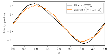
Figure 1: Time- and $(x,y)$-averaged kinetic and current helicity $z$-profiles in a typical simulation (run T06, $Rm\simeq 2800$, $Re\simeq 700$, $L_{f}=1$, $L_{z}=4$).

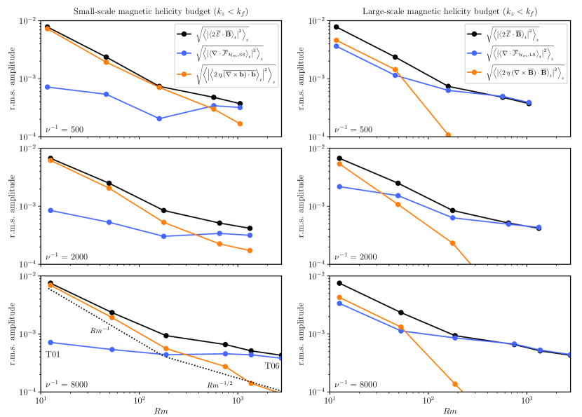
Figure 2: Small- and large-scale helicity budgets on large scales in $z$ ($k_{z}<k_{f}$) as a function of $Rm$, for different $Re$.

Run	$N_{(x,y)},N_{z}$	$\nu^{-1}$	$\eta^{-1}$	$Re$	$Rm$	$u_{\mathrm{rms}}$	$B_{\mathrm{rms}}$	$\overline{B}_{\mathrm{rms}}$
V01	$64^{2},256$	500	125	46.7	11.7	0.59	0.49	0.39
V02	$64^{2},256$	500	500	46.2	46.2	0.58	0.57	0.42
V03	$128^{2},512$	500	2000	39.9	159.7	0.50	0.54	0.21
V04	$128^{2},512$	500	8000	35.6	570.0	0.44	0.58	0.14
V05	$256^{2},1024$	500	16000	32.9	1054.0	0.41	0.59	0.12
M01	$64^{2},256$	2000	125	201.2	12.6	0.63	0.51	0.42
M02	$64^{2},256$	2000	500	197.6	49.4	0.62	0.56	0.38
M03	$128^{2},512$	2000	2000	177.0	177.0	0.56	0.59	0.32
M04	$128^{2},512$	2000	8000	163.3	653.2	0.51	0.60	0.18
M05	$256^{2},1024$	2000	16000	165.9	1327.5	0.52	0.60	0.12
T01	$128^{2},512$	8000	125	804.4	12.6	0.63	0.48	0.37
T02	$128^{2},512$	8000	500	846.6	52.9	0.66	0.58	0.42
T03	$128^{2},512$	8000	2000	749.3	187.3	0.59	0.58	0.25
T04	$128^{2},512$	8000	8000	748.1	748.1	0.58	0.60	0.16
T05	$256^{2},1024$	8000	16000	683.4	1366.8	0.54	0.63	0.17
T06	$512^{2},2048$	8000	32000	694.5	2778.0	0.55	0.62	0.12

Table 1: Run index. $L_{x},L_{y}=L_{f}=L_{z}/4$ for all runs.

We performed a parametric study for different Reynolds $Re=u_{\mathrm{rms}}/(k_{f}\nu)$ and magnetic Reynolds numbers $Rm=u_{\mathrm{rms}}/(k_{f}\eta)$, where $u_{\mathrm{rms}}$ is the r.m.s. flow amplitude (over time and space). We set $\omega_{f}=1$, $A_{f}=0.1$, $L_{f}=1$, and $L_{z}=4L_{f}$ in all simulations to ensure a minimal scale separation between the turbulence forcing scale and the scales of the helical inhomogeneity and emergent large-scale statistical dynamics. Each run (Tab. 1) was integrated for at least 50 forcing times $2\pi/\omega_{f}$ (175-200 flow turnover times $L_{f}/u_{\mathrm{rms}}$). To isolate the weaker slow, large-scale signal from the fast turbulent noise, the magnitude of each term in equations (2)-(3) was estimated by Fourier-filtering them on $z$-scales larger than the forcing scale ($k_{z}<k_{f}$), then taking the r.m.s. values (over $z$) of their time-averages after initial growth of the dynamo.

Results.

Helicity bugdgets as a function of $Rm$ are shown in Fig. 2. The results are only weakly dependent on $Re$. At low $Rm$, both budgets are characterized by a balance between resistive and helical EMF terms. As $Rm$ reaches $50-100$, the large-scale budget transitions to a regime characterized by a dominant balance between the large-scale $z$-flux of large-scale helicity and EMF. However, for $Rm<300-500$, the dominant balance in the small-scale helicity budget remains between the resistive dissipation of small-scale helicity and EMF. Hence, the large-scale dynamics is still affected by resistive effects in this $Rm$ range. This regime is nevertheless interesting in that it can only be realized for non-uniform flow helicity [51]. It really takes $Rm>1000$ to reach a regime characterized by a dominant non-resistive balance in both large- and small-scale helicity budgets, the latter now being between the large-scale $z-$flux of small-scale helicity and the EMF term. A weak residual dependence of both terms on $Rm$ remains in the range of $Rm$ probed.

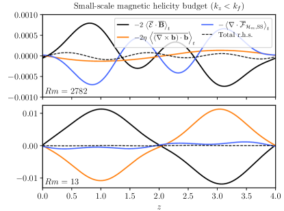
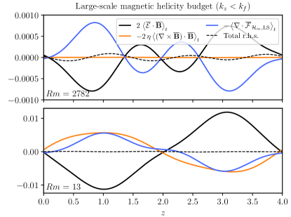
Figure 3: Time-averaged helicity budgets on scales $k_{z}<k_{f}$ (T06: $Rm\simeq 2800$, $Re\simeq 700$ ; T01: $Rm\simeq 15$, $Re\simeq 800$).

A detailed comparison, between low and large-$Rm$ runs with identical viscosity, of the time-averaged $z$-dependent quantities in equations (2)-(3), again filtered on $z$-scales larger than the flow forcing scale, is shown in Fig. 3 to make more explicit the transition between the resistively-dominated and asymptotic regimes. Estimates of the flux divergences carried out in the Coulomb gauge were always found to be in good agreement with the calculation of the (gauge-independent) r.h.s. of equations (2)-(3) at large $Rm$, as expected in a statistically steady state [50]. Hence, we are confident that the main trends reported here do not depend on our gauge choice.

Fig. 4 shows the energy of $\overline{\mathbf{B}}$ as a function of $Rm$. The results at intermediate $Rm$ are consistent with a $Rm^{-1}$ scaling, in line with theory expectations and earlier simulations [58, 52]. There is as yet no clear-cut evidence for an asymptotic regime entirely independent of $Rm$ (maybe because the small-scale helicity dissipation term only seemingly decreases slowly as $Rm^{-1/2}$ at large $Rm$), however we observe a clear deviation away of the $Rm^{-1}$ scaling for the energy of the mean-field at the largest $Re$ and $Rm$ probed. Mean-field models assuming turbulent diffusive expressions for the helicity fluxes also suggest that convergence of $\overline{B}^{2}_{\mathrm{rms}}/B^{2}_{\mathrm{rms}}$ towards an $Rm$-independent value should be slow at large $Rm$ [58, 53].

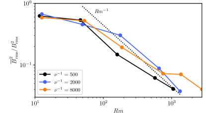
Figure 4: Time-averaged energy of $\overline{\mathbf{B}}$ relative to the total magnetic energy, as a function of $Rm$.

For our parameters, convincing access to a regime with subdominant resistive contributions required a (spectral) resolution of 512 per $L_{f}$ (run T06, $Rm\simeq 2800$, $Re\simeq 700$). The evolution of energy densities, and time-averaged energy spectra in the statistically steady state of T06 are shown in Fig. 5.

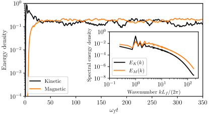
Figure 5: Evolution of kinetic and magnetic energy densities (T06: $Rm\simeq 2800$, $Re\simeq 700$). Inset: associated energy spectra in the saturated phase.

The evolutions of the large-scale field component $\overline{B}_{x}(z,t)$ and large-scale magnetic energy densities are shown in Fig. 6.

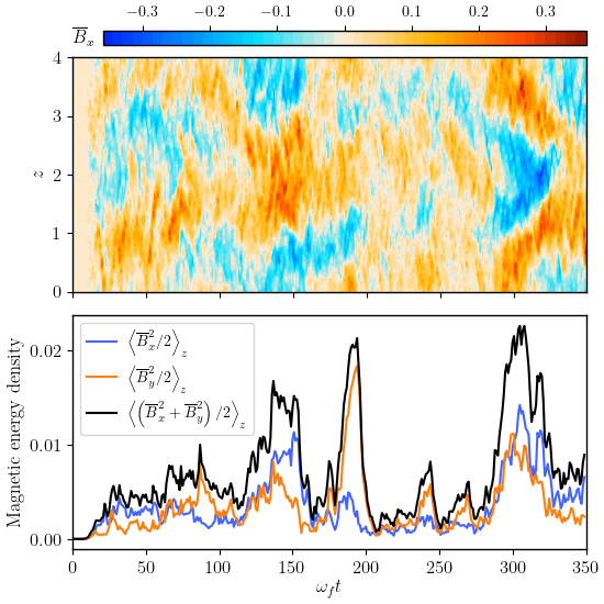
Figure 6: Evolution of (top) $\overline{B}_{x}(t,z)$ and (bottom) energy density of mean field (T06: $Rm\simeq 2800$, $Re\simeq 700$).

$\overline{\mathbf{B}}$ displays bursty oscillations, on a timescale $\sim 50-60\,\omega_{f}^{-1}$ ($\sim 30$ turnover times), that appear to propagate spatially towards the equator associated with the node of kinetic helicity at $z=2$, a likely consequence of the symmetry-breaking flow helicity profile in $z$ [58]. Snapshots at the end of the run (Fig. 7) show complex, turbulent magnetic structures with tentative nascent plasmoids typical of reconnection in nonlinear tangled magnetic fields at large $Rm$ [7, 38], e. g. at $(x,z)\simeq(0.5,0.75);(0.75,1.3);(0.8,3.2);(0.75,3.5)$. The “small-scale” horizontal structure visible in the bottom plot is the direct imprint of the forcing at $L_{f}$ and is distinct from the weaker, but larger-scale emergent statistical order in $z$ visible in Fig. 6.

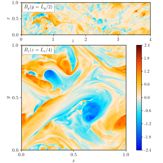
Figure 7: $(x,z)$ (top) and $(x,y)$ (bottom) out-of-plane magnetic-field snapshots (T06: $Rm\simeq 2800$, $Rm=700$).

Discussion.

Numerical results showing a similar transition in the presence of advective “wind” boundary losses of helicity have been obtained previously [50], albeit with a larger transition $Rm$ (their simulations at lower $Rm$ with no wind also hinted at solutions involving turbulent diffusive fluxes, but with different symmetries). In all cases, the strong dependence of the saturated state on $\eta$ is circumvented at large $Rm$ by non-resistive helicity fluxes. The nonlinear state achieved here, anticipated in [58, 52, 53], is particularly appealing in that it stems from a very simple inhomogeneous, hemispheric distribution of kinetic helicity also typical of rotating astrophysical systems. While the solution is dominated by small-scale fields, a clear magnetic activity pattern migrating towards the equator is present on scales larger than the flow forcing scale. Further investigations are needed to determine whether a mean shear may boost the generation of a streamwise “azimuthal” large-scale field, and how such a shear, or the transition to the low $Pm$, large $Rm$ regime typical of stellar dynamos may affect the properties of the identified travelling wave pattern.

Modelling helicity fluxes as turbulent diffusive fluxes also suggests that the transition $Rm$ (to the regime with a subdominant resistive term) scales as $(k_{f}/\overline{k})^{2}$, where $\overline{k}$, the scale of $\overline{\mathbf{B}}$, should be comparable to the helicity modulation scale [53]. If this scaling applies, something we could unfortunately not test due to limited computing resources, the asymptotic regime of large-scale astrophysical dynamos typically involving large scale-separations may be at significantly higher $Rm$ than that determined here for $L_{z}/L_{f}=4$. As global simulations are currently limited to $Rm$ of a few hundreds (also uncomfortably close to the small-scale dynamo threshold), this raises the question of their lack of asymptoticity for the foreseeable future. Our results may provide a useful reference point to assess such future simulations in this respect.

An in-depth understanding of this large-$Rm$ MHD state remains to be developed. One may be tempted to interpret it “classically” as the nonlinear outcome of an $\alpha$ effect dynamo [12, 8, 1, see also [39] for theoretical work involving helicity fluxes]. Oscillations of a weak large-scale field on top of helical turbulent MHD background also suggest a (possibly connected) phenomenological interpretation in terms of simple large-scale magnetoelastic waves in small-scale tangled fields [59]. Finally, while we may have tentatively observed reconnection plasmoids in these simulations, providing a new independent estimate of the minimal (spectral) resolution required to accomodate fast reconnection in turbulent MHD, much more numerical work will be required in the future at even higher resolution to fully characterize it, and its so far poorly-understood posible effects on large-scale magnetic field generation at asymptotically large $Rm$.

References

- Moffatt [1978] H. K. Moffatt, Magnetic field generation in electrically conducting fluids (Cambridge University Press, 1978).
- Brandenburg and Subramanian [2005] A. Brandenburg and K. Subramanian, Astrophysical magnetic fields and nonlinear dynamo theory, Phys. Rep. 417, 1 (2005).
- Shukurov [2007] A. Shukurov, Galactic dynamos, in Mathematical aspects of natural dynamos, edited by Dormy, E. and Soward, A. M. (CRC Press/Taylor & Francis, 2007) p. 313.
- Roberts and King [2013] P. H. Roberts and E. M. King, On the genesis of the Earth’s magnetism, Rep. Prog. Phys. 76, 096801 (2013).
- Charbonneau [2014] P. Charbonneau, Solar dynamo theory, Annu. Rev. Astron. Astrophys. 52, 251 (2014).
- Brun and Browning [2017] A. S. Brun and M. K. Browning, Magnetism, dynamo action and the solar-stellar connection, Living Rev. Sol. Phys. 14, 4 (2017).
- Rincon [2019] F. Rincon, Dynamo theories, J. Plasma Phys. 85, 205850401 (2019).
- Steenbeck et al. [1966] M. Steenbeck, F. Krause, and K.-H. Rädler, A calculation of the mean electromotive force in an electrically conducting fluid in turbulent motion, under the influence of Coriolis forces, Z. Naturforschung 21a, 369 (1966), english translation: P. H. Roberts, & M. Stix, report NCAR-TN/IA-60, p. 29 (1971).
- Rädler [1969a] K. H. Rädler, On the electrodynamics of turbulent fields under the influence of Coriolis forces, Monatsber. Dtsch. Akad. Wiss. Berlin 11, 194 (1969a), english translation: P. H. Roberts, & M. Stix, report NCAR-TN/IA-60, p. 291 (1971).
- Rädler [1969b] K. H. Rädler, A New Turbulent Dynamo. I., Monatsber. Dtsch. Akad. Wiss. Berlin 11, 272 (1969b), english translation: P. H. Roberts, & M. Stix, report NCAR-TN/IA-60, p. 301 (1971).
- Moffatt and Proctor [1982] H. K. Moffatt and M. R. E. Proctor, The role of the helicity spectrum function in turbulent dynamo theory, Geophys. Astrophys. Fluid Dyn. 21, 265 (1982).
- Parker [1955] E. N. Parker, Hydromagnetic dynamo models., Astrophys. J. 122, 293 (1955).
- Moffatt [1970] H. K. Moffatt, Turbulent dynamo action at low magnetic Reynolds number, J. Fluid Mech. 41, 435 (1970).
- Krause and Rädler [1980] F. Krause and K. H. Rädler, Mean-field magnetohydrodynamics and dynamo theory (Oxford: Pergamon Press, 1980).
- Meneguzzi et al. [1981] M. Meneguzzi, U. Frisch, and A. Pouquet, Helical and nonhelical turbulent dynamos, Phys. Rev. Lett. 47, 1060 (1981).
- Brandenburg [2001] A. Brandenburg, The inverse cascade and nonlinear alpha-effect in simulations of isotropic helical hydromagnetic turbulence, Astrophys. J. 550, 824 (2001).
- Brandenburg [2015] A. Brandenburg, Simulations of galactic dynamos, in Magnetic fields in diffuse media, Astrophysics and Space Science Library, Vol. 407, edited by A. Lazarian, E. M. de Gouveia Dal Pino, and C. Melioli (2015) p. 529.
- Kazantsev [1967] A. P. Kazantsev, Enhancement of a magnetic field by a conducting fluid, Zh. Eksp. Teor. Fiz. 53, 1806 (1967), english translation: Sov. Phys. JETP, 26, 1031 (1968).
- Zel’dovich et al. [1984] Y. B. Zel’dovich, A. A. Ruzmaikin, S. A. Molchanov, and D. D. Sokolov, Kinematic dynamo problem in a linear velocity field, J. Fluid Mech. 144, 1 (1984).
- Schekochihin et al. [2004] A. A. Schekochihin, S. C. Cowley, S. F. Taylor, J. L. Maron, and J. C. McWilliams, Simulations of the small-scale turbulent dynamo, Astrophys. J. 612, 276 (2004).
- Haugen et al. [2004] N. E. Haugen, A. Brandenburg, and W. Dobler, Simulations of nonhelical hydromagnetic turbulence, Phys. Rev. E 70, 016308 (2004).
- Iskakov et al. [2007] A. B. Iskakov, A. A. Schekochihin, S. C. Cowley, J. C. McWilliams, and M. R. E. Proctor, Numerical demonstration of fluctuation dynamo at low magnetic Prandtl numbers, Phys. Rev. Lett. 98, 208501 (2007).
- Kulsrud and Anderson [1992] R. M. Kulsrud and S. W. Anderson, The spectrum of random magnetic fields in the mean field dynamo theory of the galactic magnetic field, Astrophys. J. 396, 606 (1992).
- Boldyrev [2001] S. Boldyrev, A solvable model for nonlinear mean field dynamo, Astrophys. J. 562, 1081 (2001).
- Boldyrev et al. [2005] S. Boldyrev, F. Cattaneo, and R. Rosner, Magnetic-field generation in helical turbulence, Phys. Rev. Lett. 95, 255001 (2005).
- Cattaneo and Hughes [1996] F. Cattaneo and D. W. Hughes, Nonlinear saturation of the turbulent effect, Phys. Rev. E 54, R4532 (1996).
- Boozer [1993] A. H. Boozer, Magnetic helicity and dynamos, Phys. Fluids B 5, 2271 (1993).
- Bhat et al. [2016] P. Bhat, K. Subramanian, and A. Brandenburg, A unified large/small-scale dynamo in helical turbulence, Mon. Not. R. Astron. Soc. 461, 240 (2016).
- Bhat [2021] P. Bhat, Saturation of large-scale dynamo in anisotropically forced turbulence, submitted, arXiv:2108.08740 (2021).
- Loureiro et al. [2007] N. F. Loureiro, A. A. Schekochihin, and S. C. Cowley, Instability of current sheets and formation of plasmoid chains, Phys. Plasmas 14, 100703 (2007).
- Uzdensky et al. [2010] D. A. Uzdensky, N. F. Loureiro, and A. A. Schekochihin, Fast magnetic reconnection in the plasmoid-dominated regime, Phys. Rev. Lett. 105, 235002 (2010).
- Dong et al. [2018] C. Dong, L. Wang, Y.-M. Huang, L. Comisso, and A. Bhattacharjee, Role of the plasmoid instability in magnetohydrodynamic turbulence, Phys. Rev. Lett. 121, 165101 (2018).
- Eyink et al. [2011] G. L. Eyink, A. Lazarian, and E. T. Vishniac, Fast magnetic reconnection and spontaneous stochasticity, Astrophys. J. 743, 51 (2011).
- Eyink [2011] G. L. Eyink, Stochastic flux freezing and magnetic dynamo, Phys. Rev. E 83, 056405 (2011).
- Moffatt [2015] H. K. Moffatt, Magnetic relaxation and the Taylor conjecture, J. Plasma Phys. 81, 905810608 (2015).
- Moffatt [2016] H. K. Moffatt, Helicity and celestial magnetism, Proc. R. Soc. Lond. Series A 472, 20160183 (2016).
- Cattaneo et al. [2020] F. Cattaneo, G. Bodo, and S. M. Tobias, On magnetic helicity generation and transport in a nonlinear dynamo driven by a helical flow, J. Plasma Phys. 86, 905860408 (2020).
- Schekochihin [2021] A. A. Schekochihin, MHD turbulence: a biased review, submitted to J. Plasma Phys., arXiv:2010.00699 (2021).
- Ji [1999] H. Ji, Turbulent Dynamos and Magnetic Helicity, Phys. Rev. Lett. 83, 3198 (1999).
- Blackman and Field [2000] E. G. Blackman and G. B. Field, Constraints on the magnitude of in dynamo theory, Astrophys. J. 534, 984 (2000).
- Kleeorin et al. [2000] N. Kleeorin, D. Moss, I. Rogachevskii, and D. D. Sokolov, Helicity balance and steady-state strength of the dynamo generated galactic magnetic field, Astron. Astrophys. 361, L5 (2000).
- Ji and Prager [2002] H. Ji and S. C. Prager, The dynamo effects in laboratory plasmas, Magnetohydrodynamics 38, 191 (2002).
- Vishniac and Cho [2001] E. T. Vishniac and J. Cho, Magnetic helicity conservation and astrophysical dynamos, Astrophys. J. 550, 752 (2001).
- Brandenburg et al. [2002] A. Brandenburg, W. Dobler, and K. Subramanian, Magnetic helicity in stellar dynamos: new numerical experiments, Astron. Nachr. 323, 99 (2002).
- Hubbard and Brandenburg [2011] A. Hubbard and A. Brandenburg, Magnetic helicity flux in the presence of shear, Astrophys. J. 727, 11 (2011).
- Hubbard and Brandenburg [2012] A. Hubbard and A. Brandenburg, Catastrophic quenching in dynamos revisited, Astrophys. J. 748, 51 (2012).
- Brandenburg [2019] A. Brandenburg, Magnetic helicity and fluxes in an inhomogeneous alpha squared dynamo, Astron. Nachr. 339, 631 (2019).
- Brandenburg and Dobler [2001] A. Brandenburg and W. Dobler, Large scale dynamos with helicity loss through boundaries, Astron. Astrophys. 369, 329 (2001).
- Mitra et al. [2011] D. Mitra, D. Moss, R. Tavakol, and A. Brandenburg, Alleviating quenching by solar wind and meridional flows, Astron. Astrophys. 526, A138 (2011).
- Del Sordo et al. [2013] F. Del Sordo, G. Guerrero, and A. Brandenburg, Turbulent dynamos with advective magnetic helicity flux, Mon. Not. R. Astron. Soc. 429, 1686 (2013).
- Brandenburg [2001] A. Brandenburg, The inverse cascade in turbulent dynamos, in Dynamo and Dynamics, a Mathematical Challenge (Springer, 2001) p. 125.
- Mitra et al. [2010a] D. Mitra, R. Tavakol, P. J. Käpylä, and A. Brandenburg, Oscillatory migrating magnetic fields in helical turbulence in spherical domains, Astrophys. J. Lett. 719, L1 (2010a).
- Mitra et al. [2010b] D. Mitra, S. Candelaresi, P. Chatterjee, R. Tavakol, and A. Brandenburg, Equatorial magnetic helicity flux in simulations with different gauges, Astron. Nachr. 331, 130 (2010b).
- Arlt and Brandenburg [2001] R. Arlt and A. Brandenburg, Search for non-helical disc dynamos in simulations, Astron. Astrophys. 380, 359 (2001).
- Lesur and Longaretti [2007] G. Lesur and P.-Y. Longaretti, Impact of dimensionless numbers on the efficiency of magnetorotational instability induced turbulent transport, Mon. Not. R. Astron. Soc. 378, 1471 (2007).
- Galloway and Proctor [1992] D. J. Galloway and M. R. E. Proctor, Numerical calculations of fast dynamos in smooth velocity fields with realistic diffusion, Nature 356, 691 (1992).
- Tobias and Cattaneo [2013] S. M. Tobias and F. Cattaneo, Shear-driven dynamo waves at high magnetic Reynolds number, Nature 497, 463 (2013).
- Brandenburg et al. [2009] A. Brandenburg, S. Candelaresi, and P. Chatterjee, Small-scale magnetic helicity losses from a mean-field dynamo, Mon. Not. R. Astron. Soc. 398, 1414 (2009).
- Hosking et al. [2020] D. N. Hosking, A. A. Schekochihin, and S. A. Balbus, Elasticity of tangled magnetic fields, J. Plasma Phys. 86, 905860511 (2020).