Hyperbolic models for transitive topological Anosov flows in dimension three.

Abstract

We prove that every transitive topological Anosov flow on a closed $3$-manifold is orbitally equivalent to a smooth Anosov flow, preserving an ergodic smooth volume form.

1 Introduction.

A topological Anosov flow on a closed $3$-manifold is a non-singular continuous $\mathbb{R}$-action satisfying the following condition: the two partitions of the manifold into stable and unstable sets of the trajectories of the flow, induce a pair of transverse foliations that intersect along the respective trajectories.

The first family of examples in this category is the family smooth Anosov flows. A smooth flow $\psi_{t}:M\to M$ generated by a non-singular smooth vector field $X$ is said to be Anosov if its natural action on the tangent bundle of $M$ preserves a hyperbolic splitting. In this case, the stable manifold theorem of hyperbolic dynamics implies that the partitions of $M$ into stable and unstable sets of the trajectories give rise to a pair of transverse, invariant, $2$-dimensional foliations, that intersect along the trajectories of the flow. Every globally hyperbolic smooth flow is, thus, a topological Anosov flow.

A general topological Anosov flow is a continuous-time dynamical system that resembles very much a smooth Anosov flow from the point of view of topological dynamics. For instance, it is orbitally expansive and satisfy the global pseudo-orbits tracing property. The main difference between topological Anosov and smooth Anosov is not a matter of regularity; it is about the lack of hyperbolic splitting. Many of the properties of smooth Anosov flows derived from the existence of a hyperbolic splitting (e.g. $C^{1}$-structural stability, exponential contraction/expansion rates along invariant manifolds, or existence of special ergodic measures) are no longer available in the topological Anosov framework.

The main problem motivating this work is the following question:

Question 1.1.

Is every topological Anosov flow on a closed $3$-manifold orbitally equivalent to a smooth Anosov flow?

When a topological Anosov flow $(\phi_{t},M)$ is orbitally equivalent to a smooth Anosov flow $(\psi_{t},N)$, we will say that the latter is a hyperbolic model of the first.

The question above has at least two traceable origins. One is related with the construction of different examples of Anosov flows on closed $3$-manifolds, where topological Anosov flows appear as intermediate steps in a battery of 3-manifold cut-and-paste techniques called surgeries. The most paradigmatic example is the so called Fried surgery introduced in [11], a kind of Dehn surgery but adapted to the pairs (flow,$3$-manifold), which produces topological Anosov flows that are not hyperbolic in a natural way (cf. question 1.2 below).

The other is related with the study of smooth orbital equivalence classes of Anosov flow. The existence of a hyperbolic model for a given topological Anosov flow $(\phi_{t},M)$ means that it is possible to endow the manifold $M$ with a smooth atlas, such that the foliation by flow-orbits is tangent to an Anosov vector field. In this sense, topological Anosov flows can be seen as the toy models from which smooth Anosov flows can be obtained, by adding suitable smooth structures on the manifold. It is thus relevant to understand if all of these topological Anosov toy models effectively correspond with a hyperbolic dynamic. The general problem of the existence of smooth models for a given expansive dynamic has been treated in other contexts, from where it is relevant to remark the case of pseudo-Anosov homeomorphisms on closed surfaces treated in [18]. (See also [20] and [8]).

The notion of topological Anosov appears involved, as well, in recent results about classification of partially hyperbolic diffeomorphisms on $3$- manifolds. An exemple is [3], where it is conjectured an affirmative answer to question 1.1.

Recall that a flow is called transitive if there exists a dense orbit. The purpose of this work is to give a consistent proof of the following statement:

Theorem A.

Every transitive topological Anosov flow on a closed $3$- manifold admits a hyperbolic model, which in addition preserves an ergodic smooth volume form.

Some special cases of this result can be derived from the works [24] and [13], if we restrict the topology of the ambient manifold to a torus bundle or a Seifert manifold. In those works, by studying the topological properties of the invariant foliations associated with an Anosov flow, it is shown that, in each case, there is essentially one possible model: suspension of a hyperbolic automorphism of the torus or geodesic flow of a hyperbolic surface. These results extend into the context of topological Anosov (or even expansive, see [6] and [23]) and provide the existence of hyperbolic models.

Let’s explain which are the general elements for our construction of hyperbolic models of transitive topological Anosov flows.

Transitiveness and open book decompositions.

Given a flow on a closed $3$-manifold, a Birkhoff section is a compact surface, usually with non-empty boundary, immersed in the phase space in such a way that: (1) The interior of the surface is embedded and transverse to the flow lines; (2) the boundary components are periodic orbits of the flow; and (3) every orbit intersects the surface in an uniformly bounded time. These sections come equipped with a first return map defined on the interior of the surface and hence the flow is a suspension on the complement of a finite set of periodic orbits.

The joint information of a flow and an associated Birkhoff section provides what is called an open book decomposition of the $3$-manifold: in the complement of a finite union of closed curves (called the binding) the manifold is a surface bundle over the circle, with fibres homeomorphic to the interior of the Birkhoff section (called pages), and monodromy map corresponding to the first return. Apart from the closed curves in the $3$-manifold that form the binding and the monodromy onto the pages, the way in which the boundary of the pages are glued along the binding is an important information associated with the open book decomposition, that may be codified (up to isotopy) with a set of integer parameters.

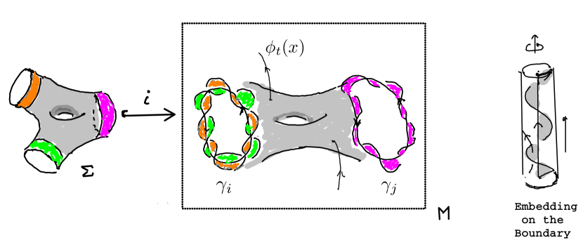
Figure 1: Birkhoff section.

In [11], Fried has proved that every transitive Anosov flow admits a Birkhoff section whose first return map is pseudo-Anosov (in a non-closed surface). This extraordinary fact, later generalized by Brunella to any transitive expansive flow in [4], opens the possibility of reducing part of the analysis of transitive Anosov flows to the theory of pseudo-Anosov homeomorphisms on surfaces and open book decompositions. Observe that transitivity is a necessary condition for the existence of a Birkhoff section, since the first return is pseudo-Anosov and hence transitive.

From a Birkhoff section associated with a topological Anosov flow it is possible to derive many interesting informations about the flow and the topology of the ambient space. To cite some examples, it is possible to construct Markov partitions ([4]), to determine the topology the orbit space associated with the flow ([10]), or even to derive geometrical properties of the ambient manifold. In addition, Birkhoff sections give a good framework for understanding and working with Fried surgeries.

We will make use of Birkhoff sections to prove theorem A. In doing this, we will be confronted with the problem of determining the orbital equivalence class of a topological Anosov flow starting from the data associated with a Birkhoff section. There is a well-known property in surface dynamics, which states that two isotopic pseudo-Anosov homeomorphisms on a closed surface are conjugated by a homeomorphism isotopic to the identity. In turn, this property means that the conjugacy class of a pseudo-Anosov in a closed surface is determined by the action of the homeomorphism on the fundamental group of the space. We will show that:

Theorem B (Theorem 3.9).

The orbital equivalence class of a transitive topological Anosov flow on a closed $3$-manifold is completely determined by the following data associated with a Birkhoff section:

1. The action of the first return map on the fundamental group of the Birkhoff section,

2. The combinatorial data associated with the embedding near the boundary components.

This theorem can be interpreted as an extension of the former property of pseudo-Anosov homeomorphisms into the context of expansive flows.

The main difficulty in proving this theorem can be explained as follows: Given two non-singular flows equipped with Birkhoff sections, if the first return maps (which are defined only on the interior of a compact surface) are conjugated, then we can use this conjugation to produce an orbital equivalence between the two flows, only defined in the complement of finite sets of periodic orbits. For extending the equivalence onto the periodic orbits on the boundary, there is an essential obstruction coming from the fact that the homeomorphism which conjugates the first return maps, in general, does not extend continuously onto the boundary of the sections. In our case, the corresponding first return applications are pseudo-Anosov but, for instance, it is not true that the action on the fundamental group determines the conjugacy class of a pseudo-Anosov homeomorphism in a surface with boundary (cf. section 2.4).

To overcome this issue, we have based our proof of theorem B on techniques coming from [2]. In that work they provide many tools for the analysis of the germ of a hyperbolic flow in the neighbourhood of a boundary component of an immersed Birkhoff section. When the Birkhoff section is nicely embedded in the $3$-manifold, a property that they call tame, it is possible to reconstruct the germ of the periodic orbit as a function of the first return map on the interior of the surface.

Construction of the hyperbolic models.

One strategy for the problem of finding a smooth representative of a given expansive dynamical systems is as follows: First, by some modification process construct a smooth model expected to be equivalent to the original one; and second, prove that the smooth model is actually equivalent to the original dynamical system by some stability argument. We can put this in practice in the case of transitive topological Anosov flows due to the existence of Birkhoff sections.

Since in the complement of a finite set of periodic orbits the flow is orbitally equivalent to the suspension of a pseudo-Anosov map on a non-closed surface, we can endow this open and dense set with a smooth transversally affine atlas and a Riemannian metric, such that the action of the flow preserves a uniformly hyperbolic splitting in an open manifold. These smooth structures will be called almost Anosov structures.

Each Birkhoff section produces an atlas like the previous one, only defined in the complement of the boundary orbits. It is not clear whether such a smooth atlas can be extended along the boundary of the section, in such a way that the original topological Anosov flow becomes smooth and preserves a hyperbolic splitting.

Question 1.2.

Let $(\phi_{t},M)$ be a transitive topological Anosov flow equipped with an almost-Anosov structure in the complement of a finite set of periodic orbits $\Gamma$ (cf. section 2.4). Does it exist a $C^{r}$-smooth Anosov flow $(\psi_{t},N)$, where $r\geq 1$, together with an orbital equivalence $H:(\phi_{t},M)\to(\psi_{t},N)$, such that the restriction of $H$ onto $M\backslash\Gamma$ is a diffeomorphism onto its image in $N$ ?

Beyond the possibility of extending or not one of this structures onto the whole manifold, we will construct a hyperbolic model of a transitive topological Anosov flow $(\phi_{t},M)$ completing the following steps:

Sketch of proof of theorem A:

1. By making a Goodman-like surgery (cf. [14]) of an almost-Anosov structure in a neighbourhood of the singular orbits, we construct a volume preserving smooth flow $\psi_{t}:N\to N$, where $N$ is a smooth manifold homeomorphic to $M$. Then, using the so-called cone field criterion (cf. [18]), we will show that this flow preserves a uniformly hyperbolic splitting.

2. We will show that both $(\phi_{t},N)$ and $(\psi_{t},N)$ are equipped with Birkhoff sections satisfying the criterion for orbital equivalence stated in theorem B.

Remark 1.3.

We find a simmilar technique in the construction of smooth models of pseudo-Anosov homeomorphisms given in [12]. Observe that as a direct consequence of its definition, a pseudo-Anosov homeomorphism is smooth (affine) in the complement of a finite singular set. The construction of the smooth models in [12] is done by modifying the given pseudo-Anosov map in a neighbourhood of its singularities and then showing equivalence. But to show equivalence between the two is not at all direct. (Remark that the pseudo-Anosov homeomorphisms are not structurally stable.) In general, a homeomorphism conjugating two pseudo-Anosov homeomorphisms is different from the identity on a big open set, no matter how close the pseudo-Anosov are in the $C^{0}$-topology.

A similar phenomenon occurs in the construction in theorem A. The surgery that we will apply is contained in a small neighbourhood of a finite set of periodic orbits. But the equivalence between the two flows will be, in general, different from the identity in a big open set. We refer to remark 3.8 below and to the discussion in page 80, proposition 3.16 of [25].

Organization of the paper.

The work is organized as follows: In section 2 we summarize the basic definitions, properties and general results that will be needed along the work. In section 3 we state and prove theorem B. In section 4 we describe a normal form of an almost-Anosov atlas around a singular orbit, that will be used in the construction of the hyperbolic models. Finally, in section 5, we give the proof of theorem A.

Acknowledgements.

The results presented in this work are a continuation of previous ones obtained by M. Brunella, C. Bonatti, F. Béguin and B. Yu., and were developed in the course of the PhD thesis of the author. We are infinitely grateful to C. Bonatti, who has introduced us into these beautiful questions and techniques. We also want to thank T. Barbot, F. Béguin, P. Dehornoy, S. Fenley, R. Potrie, F. R. Hertz and B. Yu for many helpful conversations during the preparation of the thesis.

2 Preliminaries.

This section contains the preliminary results and definitions that we will need later about flows and orbital equivalence (2.1), transverse sections and first return maps (2.2), expansive flows (2.3), and pseudo-Anosov homeomorphisms on surfaces (2.4).

2.1 Flows and orbital equivalence.

Let $(\phi_{t},M)$ be a non-singular continuous flow on a $3$-manifold $M$. The flow is said to be regular if the associated partition into orbits is a one dimensional foliation of $M$. In this case, each orbit is an immersed $1$-dimensional topological submanifold. In general, we will say that a subset of a manifold is regular if it is a topological submanifold.

The action at time $t\in\mathbb{R}$ of the flow over a point $x\in M$ will be indistinctly denoted by $\phi_{t}(x)$ or $\phi(t,x)$. Given two points $x,y\in M$ such that $y=\phi_{t}(x)$ for some $t>0$, we will denote by $[x,y]$ the orbit segment $[x,y]=\{\phi_{s}(x):0\leq s\leq t\}.$ Since we consider non-singular flows (i.e. orbits not reduced to singletons) observe that this segments are never reduced to points. The orbit of $x$ under the flow $\phi_{t}$ will be denoted by $\mathcal{O}(x)$, and we will use $\mathcal{O}^{+}(x)$ and $\mathcal{O}^{-}(x)$ to denote the positive and negative semi-orbits respectively. Observe that the orbits of a flow are naturally oriented by the direction of the flow. Given a non empty open set $U\subset M$ and a point $x\in U$ we will denote by $\mathcal{O}_{U}(x)$ the connected component of $\mathcal{O}(x)\cap U$ that contains $x$. The partition of the phase space by $\phi_{t}$-orbits induces a $1$-dimensional oriented foliation that we simply denote by $\mathcal{O}$, and we use $\mathcal{O}_{U}$ for the induced foliation on any non-empty open subset $U\subset M$.

We recall that if $X$ is a non-singular vector field of class $C^{k}$ in $M$, where $k\geq 1$, then the flow $\phi_{t}$ associated to the system of ordinary differential equations $\dot{x}=X(x)$ is a non-singular flow of class $C^{k}$. In this case, the foliation by flow orbits is of class $C^{k}$ and its leaves are immersed $1$-dimensional manifolds tangent to the vectorfield $X$.

For $i=1,2$ let $\phi_{t}^{i}:M_{i}\to M_{i}$ be a regular flow of class $C^{k}$ on a manifold $M_{i}$, where $k\geq 0$.

Definition 2.1 (Orbital equivalence).

The flows $(\phi_{t}^{1},M_{1})$ and $(\phi_{t}^{2},M_{2})$ are $C^{r}$-orbitally equivalent, where $r\geq 0$, if there exists a $C^{r}$-diffeomorphism $H:M_{1}\to M_{2}$ such that, for every $x\in M_{1}$, it sends the orbit $\mathcal{O}^{1}(x)$ homeomorphically onto the orbit $\mathcal{O}^{2}(H(x))$, preserving the orientation of these orbits. We denote it by

$$H:(\phi_{t}^{1},M_{1})\to(\phi_{t}^{2},M_{2}).$$

Remark.

When we use the word orbital equivalence without making any reference to the regularity degree $r\geq 0$, it must be understood that $r=0$, unless specified. This is, we just care about homeomorphisms preserving the oriented foliations by orbit segments, no matter the degree of regularity of the flows.

For technical reasons, we will be also interested in a weaker notion that we explain here: Consider a non-empty open subset $U\subset M$. The foliation by $\phi_{t}$-orbits on $M$ induces a foliation on $U$ but, in general, the action $\mathbb{R}\times M\to M$ provided by $\phi_{t}$ does not restrict onto an $\mathbb{R}$-action on the set $U$. Instead, what we obtain is a pseudo-flow on $U$. That is, a map $(t,x)\mapsto\phi_{t}(x)$ defined for some couples $(t,x)\in\mathbb{R}\times U$. This pseudo-flow generates a partition of $U$ into orbits, which coincides with the foliation $\mathcal{O}_{U}$ previously defined. This restriction pseudo-flow will be simply denoted by $(\phi_{t},U)$.

For each $i=1,2$ consider a non-empty open subset $U_{i}\subset M_{i}$.

Definition 2.2 (Local orbital equivalence).

The pseudo-flows $(\phi_{t}^{1},U_{1})$ and $(\phi_{t}^{2},U_{2})$ are $C^{r}$-locally orbitally equivalent, where $r\geq 0$, if there exists a $C^{r}$-diffeomorphism $H:U_{1}\to U_{2}$ such that, for every $x\in U_{1}$, it sends the orbit $\mathcal{O}_{U_{1}}^{1}(x)$ homeomorphically onto the orbit $\mathcal{O}_{U_{2}}^{2}(H(x))$, preserving the orientation of these orbits. We denote it by

$$H:(\phi_{t}^{1},U_{1})\to(\phi_{t}^{2},U_{2}).$$

If $\gamma$ is a periodic orbit of $(\phi_{t},M)$ and $W,\ W^{\prime}$ are two neighbourhoods of $\gamma$, the pseudo-flows obtained by restriction onto these sets are the same, in the sense that they coincide over their common domain of definition $W\cap W^{\prime}$. The germ of $\phi_{t}$ at $\gamma$ is the equivalence class of the pseudo-flows $\{(\phi_{t},W):W\text{ neighbourhood of }\gamma\}$ under this relation, and we denote it by $(\phi_{t},M)_{\gamma}$ or $(\phi_{t},W)_{\gamma}$.

For $i=1,2$, consider a periodic orbit $\gamma_{i}$ of $(\phi_{t}^{i},M_{i})$.

Definition 2.3 (Local orbital equivalence of germs).

The two germs $(\phi_{t}^{1},M_{1})_{\gamma_{1}}$ and $(\phi_{t}^{2},M_{2})_{\gamma_{2}}$ are $C^{r}$-locally orbitally equivalent, where $r\geq 0$, if there exists a $C^{r}$-local orbital equivalence $H:(\phi_{t}^{1},W_{1})\to(\phi_{t}^{2},W_{2})$ defined between some neighbourhoods $W_{i}$ of $\gamma_{i}$. We denote it by

$$H:(\phi_{t}^{1},W_{1})_{\gamma_{1}}\to(\phi_{t}^{2},W_{2})_{\gamma_{2}}.$$

If an orbital equivalence $H:(\phi_{t}^{1},M_{1})\to(\phi_{t}^{2},M_{2})$ satisfies in addition that $\phi_{t}^{2}(H(x))=H(\phi_{t}^{1}(x))$, for every $x\in M_{1}$ and $t\in\mathbb{R}$, we say that $H$ is a conjugation of flows. In the case where the flows $(\phi_{t}^{i},M_{i})$ are generated by a vector field $X_{i}$ of class $C^{1}$ and the conjugation is at least $C^{1}$, then conjugation between flows is equivalent to the condition

$$X_{2}(z)=H_{*}(X_{1})(z)=DH(H^{-1}(z))\cdot X_{1}(H^{-1}(z)),\ \text{ for all }z\in U_{2}.$$

The same considerations apply in the case of local orbital equivalence and pseudo-flows.

2.2 Transverse sections and first return map.

Let $\phi_{t}:M\to M$ be a non-singular regular flow on a 3-manifold $M$.

Definition 2.4 (Transverse section).

A transverse section for the flow $\phi_{t}$ is a boundaryless, regular, embedded surface $\Sigma\subset M$, satisfying that:

1. The surface $\Sigma$ is topologically transverse to the flow lines. That is, $\forall\ x\in\Sigma$ there exists a neighbourhood $W$ of $x$ inside $M$ and some $\delta>0$ such that:

   • $\Sigma\cap W$ is connected and $W\backslash\Sigma$ has two connected components;

   • $\Sigma\cap[\phi_{-\delta}(x),\phi_{\delta}(x)]=\{x\}$ and it is verified that $\textsl{int}\left([\phi_{-\delta}(x),x]\right)$ is contained in one component of $W\backslash\Sigma$ and $\textsl{int}\left([x,\phi_{\delta}(x)]\right)$ is contained in the other.

2. The surface is proper with respect to the flow lines. That is, every compact orbit segment $[\phi_{t_{1}}(x),\phi_{t_{2}}(x)]$ intersects $\Sigma$ in a compact set, where $t_{1},t_{2}\in\mathbb{R}$ and $x\in M$.

Observe that conditions $(i)$ and $(ii)$ in the definition actually imply that every compact orbit segment cuts the transverse section in a finite set. Let $\Sigma\subset M$ be a transverse section for a flow $\phi_{t}$ and assume that there exists a non empty open subset $U\subset\Sigma$ where there is a well defined first return map $P:U\to\Sigma$. That is, for every $x\in U$ there exists $\tau(x)=\min\{t>0:\phi_{t}(x)\in\Sigma\}$ and

• The function $\tau:U\to(0,+\infty)$ is continuous,

• The first return map is given by $P(x)=\phi_{\tau(x)}(x)$.

If $x$ is a point in $\Sigma$ satisfying that there exists some $t>0$ such that $\phi_{t}(x)\in\Sigma$, then from the continuity of the flow it follows that there exists a first return map defined in a neighbourhood of $x$. In fact, a first return map as above is always a homeomorphism from its domain onto its image. Moreover, as it follows from the implicit function theorem, it is a $C^{l}$-diffeomorphism, where $l$ is the minimum between the regularities of $\phi_{t}$ and $\Sigma$. We will use the following definition:

Figure 2: First return saturation $\mathcal{U}$ of the open set $U\subset\Sigma$.

Definition 2.5.

The first return saturation of $U$ is the set

$$\mathcal{U}=\{x\in M:\exists\ t\leq 0\text{ such that }\phi_{t}(x)\in U\text{ and }\textsl{int}\left([\phi_{t}(x),x]\right)\cap\Sigma=\emptyset\}.$$

This set is the union of all the compact orbits segments joining each point in $U$ with its first return to $\Sigma$, as we see in figure 2. For every $x\in\mathcal{U}$ there exists $u\in U$ and $v=P(u)\in\Sigma$ such that $x\in[u,v]$, so we define $\sigma(x)=[u,v]$. The following lemma will be used several times in what follows.

Lemma 2.6 (See [25]).

Consider two continuous flows $\phi^{i}_{t}:M_{i}\to M_{i}$, $i=1,2$. Let $\Sigma_{i}\subset M_{i}$ be a transverse section for each flow and assume there exists a first return map $P_{i}:U_{i}\to\Sigma_{i}$ defined in an open set $U_{i}\subset\Sigma_{i}$. If there exists a homeomorphism $h:\Sigma_{1}\to\Sigma_{2}$ such that $h(U_{1})=U_{2}$ and $h\circ P_{1}(x)=P_{2}\circ h(x)$, $\forall$ $x\in U_{1}$, then there exists a homeomorphism $H:\mathcal{U}_{1}\to\mathcal{U}_{2}$ such that:

1. For every point $x\in\mathcal{U}_{1}$ the map $H$ takes the orbit segment $\mathcal{O}_{\mathcal{U}_{1}}(x)$ onto $\mathcal{O}_{\mathcal{U}_{2}}(H(x))$,

2. The restriction map $H|_{U_{1}}$ coincides with $h|_{U_{1}}$.

A global transverse section $\Sigma$ for $(\phi_{t},M)$ is a transverse section that is properly embedded in $M$ and for which there exists $T>0$ such that $[x,\phi_{T}(x)]\cap\Sigma\neq\emptyset$, for every $x\in M$. In this case, the first return map is a homeomorphism $P_{\Sigma}:\Sigma\to\Sigma$. Given a periodic orbit $\gamma$ of the flow, a local transverse section at $\gamma$ is a transverse section $D$, homeomorphic to a disk, such that $\{x_{0}\}=\gamma\cap D$ contains exactly one point. Given a local transverse section $D$ there always exists a neighbourhood $U\subset D$ of $x_{0}$ and a first return map $P_{D}:U\to D$ that fixes $x_{0}$. The following statement is a consequence of lemma 2.6 above.

Proposition 2.7 (See [25]).

Let $\phi^{i}_{t}:M_{i}\to M_{i}$, $i=1,2$, be two non-singular continuous flows.

1. Assume there exists a global transverse section $\Sigma_{i}$ for each flow $\phi^{i}_{t}$ and let $P_{i}:\Sigma_{i}\to\Sigma_{i}$ be the first return map. If there exists a homeomorphism $h:\Sigma_{1}\to\Sigma_{2}$ such that $h\circ P_{1}=P_{2}\circ h$, then there exists a homeomorphism $H:M_{1}\to M_{2}$ such that:

   1. $H$ is an orbital equivalence between the flows,

   2. $H|_{\Sigma}=h$.

2. Let $\gamma_{i}$ be a periodic orbit of each flow $\phi_{t}^{i}$, $D_{i}$ a local transverse section and $P_{D_{i}}:U_{i}\to D_{i}$ a first return map defined in a neighbourhood $U_{i}\subset D_{i}$ of the intersection point $x_{i}=\gamma_{i}\cap D_{i}$. If there is a homeomorphism $h:D_{1}\to D_{2}$ such that $h(U_{1})\subset U_{2}$ and $h\circ P_{D_{1}}(x)=P_{D_{2}}\circ h(x)$, $\forall$ $x\in U_{1}$, then there exists a tubular neighbourhood $W_{i}$ of each $\gamma_{i}$ and a homeomorphism $H:W_{1}\to W_{2}$ such that:

   1. $H$ is a local orbital equivalence between the respective germs at each $\gamma_{i}$,

   2. $H|_{D_{1}\cap W_{1}}=h|_{D_{1}\cap W_{1}}$.

2.3 Topological Anosov flows.

Hyperbolic splitting.

Definition 2.8 (Hyperbolic splitting).

Let $M$ be a smooth $3$-manifold equipped with a Riemannian metric $\|\cdot\|$ and let $\phi_{t}:M\to M$ be a flow generated by a non-singular $C^{k}$-vectorfield $X$, where $k\geq 1$. A hyperbolic splitting of the tangent bundle $TM$ is a decomposition as Whitney sum of three line bundles $TM=E^{s}\oplus E^{c}\oplus E^{u}$, where $E^{c}=\textsl{span}\{X\}$, satisfying that:

1. Each line bundle is invariant by the action of $D\phi_{t}:TM\to TM$,

2. There exist constants $C>0$ and $0<\lambda<1$ such that

   $$\|D\phi_{t}(x)\cdot v\|\leq C\lambda^{t}\|v\|,\ \forall\ v\in E^{s}(x),\ t\geq 0,\ x\in\Lambda;$$ (1)

   $$\|D\phi_{t}(x)\cdot v\|\leq C\lambda^{-t}\|v\|,\ \forall\ v\in E^{u}(x),\ t\leq 0,\ x\in\Lambda.$$

The bundle $E^{s}$ is called the stable bundle, $E^{u}$ is called the unstable bundle and $E^{c}$, the one who is tangent to the flow lines, is called the central bundle. The two dimensional bundles $E^{cs}=E^{s}\oplus E^{c}$, $E^{cu}=E^{c}\oplus E^{u}$ and $E^{su}=E^{s}\oplus E^{u}$ are respectively called the center-stable bundle (or cs-bundle), the center-unstable bundle (or cu-bundle) and the stable-unstable bundle (or su-bundle).

Anosov flows.

Definition 2.9 (Anosov flow).

Let $M$ be a closed smooth $3$-manifold and let $\phi_{t}:M\to M$ be a flow generated by a non-singular $C^{k}$-vectorfield $X$, where $k\geq 1$. The flow is Anosov if $TM$ it admits a hyperbolic splitting, for some given Riemannian metric on $M$.

Remark 2.10.

Observe that from the compactness of the ambient space, in the case of an Anosov flow it follows that the vectors in $E^{s}$ or $E^{u}$ will satisfy condition (1) above for any chosen Riemannian metric on $M$ and for every reparametrization of the flow, up to modifying the constants $C>0$ and $0<\lambda<1$ if necessary (cf. [18]). Thus, the definition of Anosov flow makes an auxiliary use of a Riemannian metric, but it only depends on the $C^{1}$-equivalence class of the flow. As well, it is not difficult to check that the decomposition of $TM$ must be unique and continuous.

This observation is no longer true if $M$ is not compact. In this case, condition (1) in definition 2.8 above strongly depends on the choice of Riemannian metric.

Invariant foliations.

One of the fundamental properties of Anosov flows is the integrability of its (center-)stable and (center-)unstable bundles into foliations which are preserved by the flow action, and can be merely defined by dynamical properties. This well-known property is called stable manifold theorem, see for exemple [18].

Theorem (Stable manifold theorem.).

Let $(\phi_{t},M)$ be an Anosov flow. Then each 1-dimensional bundle $E^{s}$ or $E^{u}$ is uniquely integrable, and the partition of $M$ by integral curves respectively determines a pair of 1- dimensional foliations $\mathcal{F}^{s}$ and $\mathcal{F}^{u}$, invariant by the action of the flow. Moreover, for every $x\in M$ it is satisfied that

$$\mathcal{F}^{s}(x)=W^{s}(x)=\{y\in M:\textsl{dist}(\phi_{t}(y),\phi_{t}(x))\to 0,\ t\to+\infty\},$$

$$\mathcal{F}^{u}(x)=W^{u}(x)=\{y\in M:\textsl{dist}(\phi_{t}(y),\phi_{t}(x))\to 0,\ t\to-\infty\}.$$

In addition, each of the bundles $E^{cs}$ and $E^{cu}$ is uniquely integrable into a $2$-dimensional foliation $\mathcal{F}^{cs}$ and $\mathcal{F}^{cu}$ respectively, and for every $x\in M$ it is satisfied that:

$$\mathcal{F}^{cs}(x)=\{y\in M:\exists\ s\in\mathbb{R},\text{ s.t. }\textsl{dist}(\phi_{t}(y),\phi_{t+s}(x))\to 0,\ t\to+\infty\},$$

$$\mathcal{F}^{cu}(x)=\{y\in M:\exists\ s\in\mathbb{R},\text{ s.t. }\textsl{dist}(\phi_{t}(y),\phi_{t+s}(x))\to 0,\ t\to-\infty\}.$$

Expansive flows.

Definition 2.11 (Expansivity).

Let $\phi_{t}:M\to M$ be a non-singular flow on a closed $3$-manifold. The flow is said to be orbitally expansive if for some fixed metric on $M$ and for every $\varepsilon>0$, there exists $\alpha=\alpha(\varepsilon)>0$ such that: If two points $x$, $y$ satisfy that $\textsl{dist}(\phi_{h(t)}(y),\phi_{t}(x))\leq\alpha,\ \forall\ t\in\mathbb{R},$ where $h:(\mathbb{R},0)\to(\mathbb{R},0)$ is some increasing homeomorphism, then $y=\phi_{s}(x)$ for some $|s|\leq\varepsilon$.

As before, this definition is independent of the chosen metric by compactness of the ambient space. General expansive flows on closed $3$-manifolds have been studied by Paternain, Inaba and Matsumoto. In [22] and [17] it is shown that every orbitally expansive flow is orbitally equivalent to a pseudo-Anosov flow.

This is obtained by showing that the partitions of $M$ into stable and unstable sets of the orbits, that is

$$\mathcal{W}^{s}(\mathcal{O}(x))=\{y\in M: \exists\ s\in\mathbb{R}\ \text{and repar. }h:(\mathbb{R},0)\to(\mathbb{R},0)$$

$$\text{ s.t. }\textsl{dist}(\phi_{h(t)}(y),\phi_{t+s}(x))\to 0,\ t\to+\infty\},$$

$$\mathcal{W}^{u}(\mathcal{O}(x))=\{y\in M: \exists\ s\in\mathbb{R}\ \text{and repar. }h:(\mathbb{R},0)\to(\mathbb{R},0)$$

$$\text{ s.t. }\textsl{dist}(\phi_{h(t)}(y),\phi_{t+s}(x))\to 0,\ t\to-\infty\},$$

constitute a pair of transverse foliations in $M$, possibly with singularities, which are invariant by the flow action and intersect along the flow orbits. We denoted them by $\mathcal{F}^{cs}$ and $\mathcal{F}^{cu}$ respectively. The singularities are of a special type called circle prongs, that are obtained by suspending $k$-prong multi-saddle fixed points in a disk. See [4] or the referred works for precise statement and definitions.

Topological Anosov flows.

Definition 2.12 (Topological Anosov flow).

Let $(\phi_{t},M)$ be a non-singular flow on a closed $3$- manifold. It is said to be topological Anosov if it is orbitally expansive and its invariant foliations have no singularities.

As a final remark, it is possible to see that a flow is topological Anosov if and only if it is orbitally expansive and satisfies the pseudo-orbits tracing property, since in the presence of invariant foliations then multi-saddle orbits are the only obstruction to shadowing. In general, a topological Anosov dynamical system (discrete- or continuous-time) is one that is expansive and satisfies globally the pseudo-orbits tracing property. See [1] for definitions and general properties of topological Anosov dynamical systems.

2.4 Pseudo-Anosov homeomorphisms.

Let $\Sigma$ be a closed orientable surface.

Definition 2.13.

A homeomorphism $f:\Sigma\to\Sigma$ is pseudo-Anosov if there exists a pair of transverse, $f$-invariant, foliations $\mathcal{F}^{s}$ and $\mathcal{F}^{u}$ on $\Sigma$, respectively equipped with transverse measures $\mu_{s}$ and $\mu_{u}$ and a constant $0<\lambda<1$ such that $f_{*}(\mu_{s})=\lambda^{-1}\cdot\mu_{s}$ and $f_{*}(\mu_{u})=\lambda^{-1}\cdot\mu_{u}$ The transverse measures are required to be non-atomic and with full support.

If the genus of $\Sigma$ is greater than one, then the two foliations necessarily have singularities. If this is the case, in the previous definition we just allow singularities whose local model is a $k$-prong singularity (see figure 3(a)) and with $k\geq 3$. Since the foliations must be transverse between them, then $\mathcal{F}^{s}$ and $\mathcal{F}^{u}$ share the same (finite) set of singularities, and in a small neighbourhood of each singularity the two foliations intersect as in the local model 3(b).

(a) $k$-prong singularity, $k=3$.

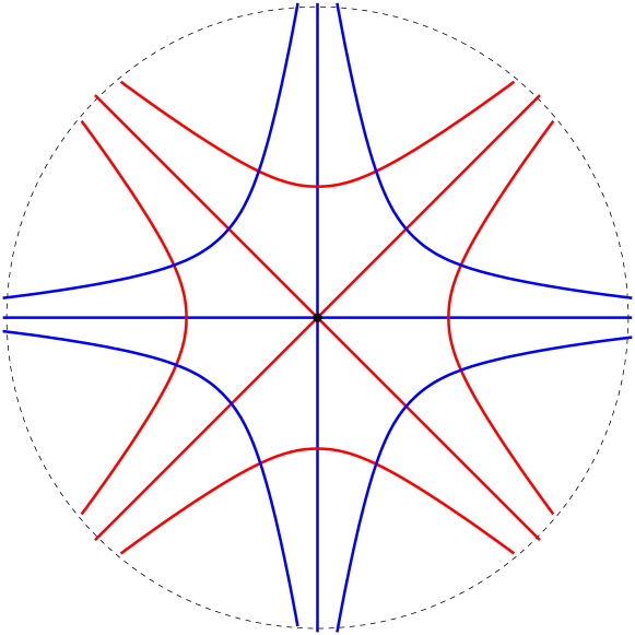
(b) Transverse foliations at $k$-prong, $k=4$.

Figure 3: Local model of $k$-prong singularities

By the Euler-Poincaré formula (see [9]), the sphere is excluded from having a pseudo-Anosov homeomorphism and in the torus the foliations are non-singular. If $\textrm{gen}(\Sigma)\geq 2$, observe that the set of singularities $\Delta$ is necessarily included in the set of periodic points of $f$.

For higher genus surfaces, pseudo-Anosov homeomorphisms can be seen as a counter-part of linear hyperbolic automorphisms of the torus. In view of the singularities, they can never be hyperbolic diffeomorphisms, but they share some properties with the latter ones. For instance, every pseudo-Anosov homeomorphism $f:\Sigma\to\Sigma$ is transitive, expansive, the set of periodic points is dense in $\Sigma$, and the topological entropy of $f$ is positive. More generally, the dynamic of a pseudo-Anosov map can be encoded using a Markovian partition constructed from its invariant foliations, as is shown in [9]. From the symbolic point of view these maps are equivalent to subshifts of finite type.

In [19] and [16], Lewowicz and Hiraide have shown that the pseudo-Anosov maps are the only expansive homeomorphisms in a closed orientable surface. More precisely, if $f:\Sigma\to\Sigma$ is an expansive homeomorphism then $\textrm{gen}(\Sigma)\geq 1$ and if $\textrm{gen}(\Sigma)=1$ then $f$ is $C^{0}$-conjugated to a linear Anosov map, and in higher genus $f$ is $C^{0}$-conjugated to some pseudo-Anosov homeomorphism.

Smooth models.

In [12], Gerber and Katok proved that every pseudo-Anosov homeomorphism $f$ on a closed surface $\Sigma$ is $C^{0}$-conjugated to some diffeomorphism $g:\Sigma\to\Sigma$, which in addition preserves an ergodic smooth measure. See also [20] for an analytic version. Let’s point out some interesting facts about this result.

If $f:\Sigma\to\Sigma$ is a pseudo-Anosov homeomorphism, then the system of transverse foliations equipped with transverse measures defines a translation atlas $\mathcal{A}_{\Delta}$ in the complement of the set of singularities $\Delta$ (see e.g. [9]). Choose some smooth atlas $\mathcal{A}$ on $\Sigma$ such that the inclusion map $(\Sigma\backslash\Delta,\mathcal{A}_{\Delta})\hookrightarrow(\Sigma,\mathcal{A})$ induces a diffeomorphism onto its image. From now on we consider $\mathcal{A}$ as a fixed smooth structure on $\Sigma$.

Directly from the construction we can see that the restriction $f:\Sigma\backslash\Delta\to\Sigma\backslash\Delta$ is a smooth diffeomorphism, and that it is not differentiable on the singular points $x\in\Delta$. In [12], proposition at page 177, it is showed that $f$ cannot be $C^{0}$-conjugated to a diffeomorphism $g:\Sigma\to\Sigma$, via a homemorphism that is a $C^{1}$-diffeomorphism except at the sigularities of $f$. This result says that singularities of the smooth atlas $\mathcal{A}_{\Delta}$ are essential for the dynamic of $f$, in the sense that it cannot be extended onto a globally defined $C^{1}$-atlas, in such a way that $f$ turns into a diffeomorphism. The principal result in [12] gives a smooth atlas $\mathcal{B}$ on $\Sigma$ such that, in the coordinates of this atlas, $f$ is a smooth diffeomorphism. Nevertheless, the atlas $\mathcal{B}$ is nowhere compatible with $\mathcal{A}_{\Delta}$.

Remark 2.14.

The principal result in the present work, theorem A, is a similar question to that treated by Gerber and Katok in the referred work, but translated into the context of topological Anosov flows. It should be noted that our procedure for constructing hyperbolic models of topological Anosov flows follows the same general strategy of that in [12].

2.4.1 Conjugacy classes of pseudo-Anosov homeomorphisms.

A remarkable property about pseudo-Anosov homeomorphisms is that if two of these maps are isotopic, then they are conjugated by a homeomorphism isotopic to the identity.

Theorem 2.15 ([9], Exposé XII, theorem 12.5).

Let $\Sigma$ be a closed orientable surface and let $f$ and $g$ be two pseudo-Anosov homeomorphisms. If $g$ is isotopic to $f$ then there exists a homeomorphism $h:\Sigma\to\Sigma$, isotopic to the identity, such that $f\circ h=h\circ g$.

This theorem, in combination with the Dehn-Nielsen-Baer theorem about mapping class groups, allows to decide if two pseudo-Anosov homeomorphisms are conjugated by looking at their actions on fundamental groups. In the following we explain this fact in the way that it will be used later. We refer to [25] for a more accurate explanation and proofs.

The action on the fundamental group.

Let $x_{0}$ be a point in $\Sigma$. Every $f\in\textrm{Homeo}(\Sigma)$ induces an automorphism of $\pi_{1}(\Sigma,x_{0})$ in the following way: Let $\beta:[0,1]\to\Sigma$ be an arc that connects $x_{0}=\beta(0)$ with $f(x_{0})=\beta(1)$. Given a class $[\gamma]\in\pi_{1}(\Sigma,x_{0})$ represented by a curve $\gamma:[0,1]\to\Sigma$ we define

$$f_{*}^{\beta}:[\gamma]\mapsto\left[\bar{\beta}\cdot f(\gamma)\cdot\beta\right],\text{ where }\bar{\beta}\text{ is }\beta\text{ parametrized with inverse sense}.$$

The map $f_{*}^{\beta}$ is a well-defined automorphism of $\pi_{1}(\Sigma,x_{0})$ which depends on the particular election of the arc $\beta$. If we choose another arc $\beta^{\prime}$ connecting $x_{0}=\beta^{\prime}(0)$ with $f(x_{0})=\beta^{\prime}(1)$, then $f_{*}^{\beta^{\prime}}=[\alpha]^{-1}\cdot f_{*}^{\beta}\cdot[\alpha]$ where $[\alpha]=[\bar{\beta}\cdot\beta^{\prime}]\in\pi_{1}(\Sigma,x_{0})$. Thus, changing the arc $\beta$ has the effect of conjugate $f_{*}^{\beta}$ by an inner automorphism of the fundamental group $\pi_{1}(\Sigma,x_{0})$.

Definition 2.16.

Given a pair of homeomorphisms $f_{i}:\Sigma_{i}\to\Sigma_{i}$, $i=1,2$, where $\Sigma_{1}$ and $\Sigma_{2}$ are two homeomorphic closed orientable surfaces, we say that $f_{1}$ and $f_{2}$ are $\pi_{1}$-conjugated if there exist points $x_{i}\in\Sigma_{i}$, induced actions $(f_{i})_{*}^{\beta_{i}}:\pi_{1}(\Sigma_{i},x_{i})\to\pi_{1}(\Sigma_{i},x_{i})$ and an isomorphism $\phi:\pi_{1}(\Sigma_{1},x_{1})\to\pi_{1}(\Sigma_{2},x_{2})$ such that $(f_{2})_{*}^{\beta_{2}}\circ\phi=\phi\circ(f_{1})_{*}^{\beta_{1}}$.

Observe that if $f_{1}$ and $f_{2}$ are $\pi_{1}$-conjugated then, for every pair of points $x_{i}$, every pair of induced actions $(f_{i})_{*}^{\beta_{i}}$ on $\pi_{1}(\Sigma_{i},x_{i})$ are conjugated by an isomorphism $\phi:\pi_{1}(\Sigma_{1},x_{1})\to\pi_{1}(\Sigma_{2},x_{2})$.

Proposition 2.17 (See [25]).

For $i=1,2$ consider a pseudo-Anosov homeomorphism $f_{i}:\Sigma_{i}\to\Sigma_{i}$ defined in a closed orientable surface $\Sigma_{i}$. If $f_{1}$ and $f_{2}$ are $\pi_{1}$-conjugated, then there exists a homeomorphism $h:\Sigma_{1}\to\Sigma_{2}$ such that $f_{2}\circ h=h\circ f_{1}$.

2.4.2 The case of punctured surfaces.

Consider two pseudo-Anosov homeomorphisms $f_{i}:\Sigma_{i}\to\Sigma_{i}$, where $i=1,2$, defined in two closed, orientable, homeomorphic surfaces. For each $f_{i}$ consider a finite collection of periodic orbits $\mathcal{O}^{i}_{1},\dots,\mathcal{O}^{i}_{N}$. That is, for each $k=1,\dots,N$,

$$\mathcal{O}^{i}_{k}=\{x^{i}_{k1},\dots,x^{i}_{kp_{k}}\}$$

where $x^{i}_{kn}=f_{i}^{n-1}(x^{i}_{k1})$ and $p_{k}\geq 1$ is the period of the orbit. We are interested in knowing when $f_{1}$ is conjugated to $f_{2}$ by a homeomorphism $h:\Sigma_{1}\to\Sigma_{2}$, with the additional property that $h$ sends each orbit $\mathcal{O}^{1}_{k}$ to the orbit $\mathcal{O}^{2}_{k}$.

A finite type punctured surface is the data of a compact surface $\Sigma$ together with a finite subset $\mathcal{O}\subset\Sigma$. In this text we just consider the case where the surface is closed. The mapping class group of the punctured surface $(\Sigma;\mathcal{O})$ is defined to be the set homeomorphisms $f:\Sigma\to\Sigma$ preserving the set $\mathcal{O}$, modulo isotopies fixing $\mathcal{O}$.

Denote by $\pi_{1}(\Sigma,x_{0};\mathcal{O})$ the fundamental group of $\Sigma\backslash\mathcal{O}$ based in a point $x_{0}$ not in $\mathcal{O}$. If $f$ is a homeomorphism of $\Sigma$ preserving $\mathcal{O}$, then it induces a permutation of this finite set as well as an action on $\pi_{1}(\Sigma,x_{0};\mathcal{O})$, uniquely defined up to conjugation by inner automorphisms.

Let $\mathcal{O}=\{x_{1},\dots,x_{R}\}$. For each of the points $x_{l}$ consider a closed curve homotopic to the puncture $x_{l}$ and joined to $x_{0}$ with an arbitrary path. This curve determines an element of $\pi_{1}(\Sigma,x_{0};\mathcal{O})$ that we denote by $c_{l}$. We denote by $\Gamma(\mathcal{O})$ the set of conjugacy classes of the elements $c_{l}$. That is,

$$\Gamma(\mathcal{O})=\{\bar{\gamma}\cdot c_{l}\cdot\gamma:\text{ where }l=1,\dots,R\text{ and }\gamma\in\pi_{1}(\Sigma,x_{0};\mathcal{O})\}.$$

The action $f_{*}$ leaves invariant the set $\Gamma(\mathcal{O})$, since it comes from a homeomorphism of the surface.

Proposition 2.18 (See [25]).

For $i=1,2$ consider a pseudo-Anosov homeomorphism $f_{i}:\Sigma_{i}\to\Sigma_{i}$ defined in a closed orientable surface $\Sigma_{i}$ and a finite collection of periodic orbits $\mathcal{O}^{i}_{1},\dots,\mathcal{O}^{i}_{N}$ of periods $p_{1},\dots,p_{N}$, respectively. Assume there exists an isomorphism

$$\phi:\pi_{1}(\Sigma_{1};\mathcal{O}^{1}_{1}\cup\dots\cup\mathcal{O}^{1}_{N})\to\pi_{1}(\Sigma_{2};\mathcal{O}^{2}_{1}\cup\dots\cup\mathcal{O}^{2}_{N})$$

such that:

1. $\phi$ conjugate the actions $(f_{i})_{*}$ induced on fundamental groups of $\Sigma_{i}\backslash\mathcal{O}^{i}_{1}\cup\cdots\cup\mathcal{O}^{i}_{N}$,

2. $\phi(\Gamma(\mathcal{O}^{1}_{k}))=\Gamma(\mathcal{O}^{2}_{k})$ for every $k=1,\dots,N$.

Then, there exists a homeomorphism $h:\Sigma_{1}\to\Sigma_{2}$ such that $f_{2}\circ h=h\circ f_{1}$ which in addition satisfies $h(\mathcal{O}^{1}_{k})=\mathcal{O}^{2}_{k}$, $\forall\ k=1,\dots,N$.

2.4.3 Pseudo-Anosov on non-closed surfaces.

We will use proposition 2.18 in the course of the proofs of theorems A and B. By the way, since we will be working with non-closed surfaces, we make some remarks in what follows. Let $\Sigma$ be a compact orientable surface.

Definition 2.19 (Pseudo-Anosov on non-closed surfaces).

Let $f:\Sigma\to\Sigma$ be a homeomorphism. Let $\widehat{\Sigma}$ the surface obtained by collapsing each boundary component into a point and let $\hat{f}$ be the corresponding induced map on the quotient. We say that $f$ is pseudo-Anosov if $\hat{f}$ is pseudo-Anosov according to definition 2.13.

Let $C$ be a boundary component of $\Sigma$ and $p\in\widehat{\Sigma}$ the point obtained after collapsing $C$. Each invariant foliation of $\hat{f}$ has a finite number of leaves which accumulate on $p$, which are usually called branches. When lifted to $\Sigma$, these branches do not necessarily converge to a point in $C$, as is depicted in figure 4(b). We say that the foliations are tame if the local model in a neighbourhood of the boundary component $C$ is as in figure 4(a). In this case, each branch converge to a point in $C$, which is necessarily periodic for $f$.

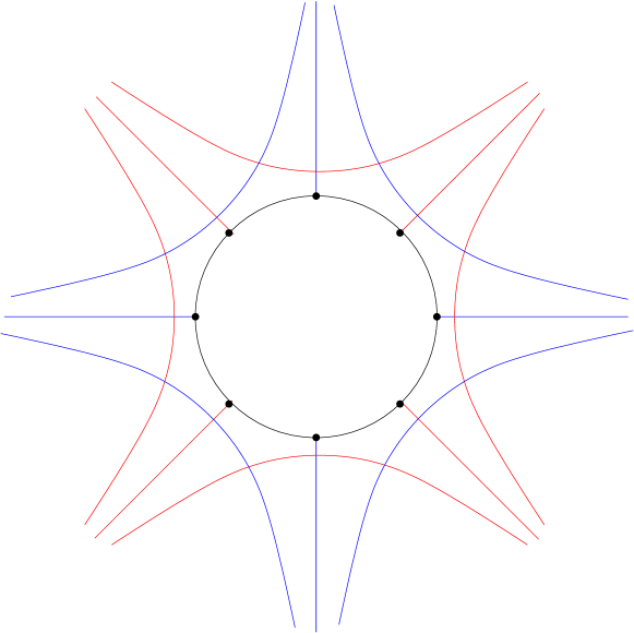
(a) Tame

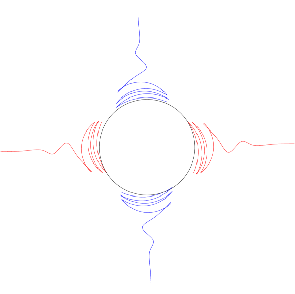
(b) Wild

Figure 4: Local model of $k$-prong singularities

Collapsing each boundary component into a point provides a semi- conjugation from $f$ to $\hat{f}$, which is actually a conjugation on the interior of the surface. So, most of the dynamical properties of $\hat{f}$ are also available for $f$. However, we want to point out the following:

Remark 2.20 (Conjugacy classes of pseudo-Anosov in non-closed surfaces.).

Theorem 2.15 as well as proposition 2.17 are no longer available in the case of non-closed surfaces.

We want to point out an obstruction to conjugacy which depends on the behaviour of the map in a neighbourhood of the boundary. We illustrate this in the following example.

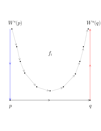
Figure 5: The homeomorphisms in example 2.21.

Example 2.21.

Consider two $C^{1}$-diffeomorphisms $f$ and $g$ defined in the band $[-1,1]\times[0,+\infty)$, whose phase portrait is as follows:

• The non-wandering set consists in the corner points $p=(-1,0)$ and $q=(1,0)$, which are saddle type hyperbolic fixed points.

• $W^{s}(p)=\{-1\}\times[0,+\infty)$,

• $W^{u}(q)=\{1\}\times[0,+\infty)$,

• The segment $[-1,1]\times\{0\}$ is a saddle connection between $p$ and $q$.

This is illustrated in figure 5. For each fixed point $x=p,q$ we have that

$$Df(x)=\begin{pmatrix}\lambda_{x}(f)&0\\ 0&\mu_{x}(f)\end{pmatrix}\text{ and }Dg(x)=\begin{pmatrix}\lambda_{x}(g)&0\\ 0&\mu_{x}(g)\end{pmatrix}.$$

Proposition.

If there exists a homeomorphism $h:[-1,1]\times[0,+\infty)\to[-1,1]\times[0,+\infty)$ such that $g\circ h=h\circ f$, then

$$\frac{\log(\mu_{q}(f))}{\log(\mu_{p}(f))}=\frac{\log(\mu_{q}(g))}{\log(\mu_{p}(g))}.$$

In particular, general homeomorphisms (even $C^{1}$-diffeomorphisms) whose phase portrait is as in example 2.21 are not $C^{0}$-conjugated. Observe that there always exists a conjugation between these dynamics in the complement of the segment $[-1,1]\times\{0\}$. This can be seen by dividing the band into adequate fundamental domains for the action of each map. The obstruction appears when we try to extend the conjugation to the segment that connects the two saddles.

This dynamical behaviour is what we encounter in the neighbourhood of a boundary component of a surface $\Sigma$, when we look at the action of a pseudo-Anosov map. If we choose a power of $f$ that fixes the boundary component, then we can decompose a neighbourhood of this component into a finite number of bands homeomorphic to $[-1,1]\times[0,+\infty)$ where the dynamic looks like in the example 2.21. As a final remark, observe that if $\hat{f}:\widehat{\Sigma}\to\widehat{\Sigma}$ is a pseudo-Anosov in a closed surface, we can construct a pseudo-Anosov $f:\Sigma\to\Sigma$ in a non closed surface by blowing up $\hat{f}$ along a periodic orbit. But, in view of 2.21, different ways of blowing up could lead to non-conjugated maps, even if all the actions on $\pi_{1}(\Sigma)$ are the same.

3 Birkhoff sections and orbital equivalence classes.

Let $\phi_{t}:M\to M$ be a transitive topological Anosov flow on a closed $3$-manifold.

Definition 3.1.

A Birkhoff section for the flow $(\phi_{t},M)$ is an immersion $\iota:(\Sigma,\partial\Sigma)\to(M,\Gamma)$, where $\Sigma$ is a compact surface, sending $\partial\Sigma$ onto a finite union $\Gamma$ of periodic orbits of $\phi_{t}$, such that:

1. The restriction of $\iota$ to each component of $\partial\Sigma$ is a covering map onto a closed curve in $\Gamma$.

2. The restriction of $\iota$ to the interior $\mathring{\Sigma}$ is an embedding inside $M\backslash\Gamma$, and the submanifold $\iota(\mathring{\Sigma})$ is transverse to the foliation by trajectories of the flow.

3. $\exists$ a real number $T>0$ such that $[x,\phi_{T}(x)]\cap\iota\left(\Sigma\right)\neq\emptyset$, $\forall$ $x\in M$.

We will indistinctly use the notation $\mathring{\Sigma}$ to denote $\Sigma\backslash\partial\Sigma$ or to denote its inclusion $\iota(\mathring{\Sigma})$ inside the open manifold $M_{\Gamma}\coloneqq M\backslash\Gamma$. Conditions $2.$ and $3.$ above imply that there is a well-defined first return map $P:\mathring{\Sigma}\to\mathring{\Sigma}$, which is a homeomorphism of the form $x\mapsto P(x)=\phi(\tau(x),x)$, for some positive and bounded continuous function $\tau:\mathring{\Sigma}\to\mathbb{R}^{+}$. In particular, the surface $\mathring{\Sigma}$ is a global transverse section for the flow $\phi_{t}$ restricted to $M_{\Gamma}$. Hence, $(\phi_{t},M_{\Gamma})$ is topologically equivalent to the suspension flow generated by $P:\mathring{\Sigma}\to\mathring{\Sigma}$ (cf. proposition 2.7).

The main connexion between transitive expansive flows and Birkhoff sections is given by the following theorem:

Theorem 3.2.

(Fried [11], Brunella [4]) Every transitive and orbitally expansive non-singular continuous flow in a compact $3$-manifold admits a Birkhoff section. Moreover, the first return map is obtained from a pseudo-Anosov homeomorphism on a closed surface, by removing a finite set of periodic orbits.

It turns out that the orbital equivalence class of a transitive topological Anosov flow is completely determined by the action of the first return map on a given Birkhoff section, and the homotopy class of the embedding of the surface in the $3$-manifold in a neighbourhood of the boundary. This is the content of theorem 3.9 (theorem B) below, and all this section is devoted to prove it. Before, we state the main definitions related to Birkhoff sections.

Homological coordinates near the boundary.

Denote by $\gamma_{1},\dots,\gamma_{k}$ the periodic orbits in $\Gamma$. Since the flow is topological Anosov, the germ of the flow in a neighbourhood of any curve $\gamma_{i}$ is equivalent to the suspension of a linear transformation of the plane, given by a diagonal matrix with eigenvalues $\lambda,\mu$ satisfying $0<|\lambda|<1<|\mu|$. The local invariant manifolds $W^{s}_{loc}(\gamma_{i})$ and $W^{u}_{loc}(\gamma_{i})$ are then homeomorphic to cylinders or Möbius bands, according to the signature of the eigenvalues. We say that $\gamma_{i}$ is a saddle type periodic orbit.

Remark 3.3.

As it is shown in [4], it is always possible to find Birkhoff sections satisfying the following additional hypothesis:

• Each $\gamma_{i}\in\Gamma$ is a saddle type periodic orbit whose local invariant manifolds are orientable.

In this statement it is implicit that a topological Anosov flow always has periodic orbits with orientable invariant manifolds, and the statement holds for general transitive expansive flows as well.

From now on, we will always work with Birkhoff sections under the previous condition. The preimage by $\iota$ of each $\gamma_{i}$ may consists in many boundary components of $\Sigma$. Let’s denote the components of $\iota^{-1}(\gamma_{i})$ by $C^{i}_{1},\dots,C^{i}_{p_{i}}$, in order to have

$$\partial\Sigma=C_{1}^{1}\cup\cdots\cup C_{p_{1}}^{1}\cup\cdots\cup C_{1}^{n}\cup\cdots\cup C_{p_{n}}^{n}.$$ (2)

Definition 3.4.

We say that $p_{i}=p_{i}(\gamma_{i},\Sigma)$ is the number of connected components at $\gamma_{i}$, $i=1,\dots,k$.

For each $\gamma_{i}$ consider a (small) tubular neighbourhood $W_{i}$ of $\gamma_{i}$. Since we assume that $M$ is an oriented manifold, each $W_{i}$ is and oriented open set. We will regard $\gamma_{i}$ as an oriented closed curve, the orientation being provided by the forward-time action of the flow. The local invariant manifolds give a frame along the oriented closed curve $\gamma_{i}$, that may be used to define a meridian/longitude basis of the homology of the punctured neighbourhood $W_{i}\backslash\gamma_{i}$. More precisely,

1. Longitude: Let $\beta$ be an oriented simple closed curve contained in $W^{u}_{loc}(\gamma_{i})\cap(W_{i}\backslash\gamma_{i})$, that is orientation preserving isotopic to $\gamma_{i}$ inside the cylinder $W^{u}_{loc}(\gamma_{i})$. We call longitude to the homology class

   $$b=[\beta]\in H_{1}(W_{i}\backslash\gamma_{i}).$$

2. Meridian: Let $\alpha\subset W_{i}\backslash\gamma_{i}$ be a simple closed curve that is the boundary of an embedded closed disk $D\subset W_{i}$, which is transverse to $\gamma_{i}$ and intersects it in exactly one point. Here, the orientation in $D$ is induced by the co-orientation associated with $\gamma_{i}$, and $\alpha=\partial D$ is endowed with the boundary orientation. We call meridian to the homology class

   $$a=[\alpha]\in H_{1}(W_{i}\backslash\gamma_{i}).$$

Figure 6: Meridian/longitude basis of a punctured tubular neighbourhood $W_{i}\backslash\gamma_{i}$.

If the neighbourhood $W_{i}$ is small enough, then $(W_{i}\backslash\gamma_{i})\cap\Sigma$ splits as $p_{i}$ different annuli $B_{1}^{i},\dots,B_{p_{i}}^{i}$ properly embedded in the punctured solid torus $W_{i}\backslash\gamma_{i}$, and pairwise isotopic. Let $\sigma\subset B_{j}^{i}\backslash\gamma_{i}$ be a simple closed curve homotopic to $\gamma_{i}$ inside $B_{j}^{i}$, bounding a band $A\subset B_{j}^{i}$ such that $\partial A=\gamma_{i}\cup\sigma$. The band $A$ is co-oriented by the flow and hence defines a boundary orientation on $\sigma$. The coordinates of $[\sigma]$ in the meridian-longitude basis $\{a,b\}$ of $H_{1}(W_{i}\backslash\gamma_{i})$ are two integers $n=n(\gamma_{i},\Sigma)$ and $m=m(\gamma_{i},\Sigma)$ satisfying that

$$[\sigma]=n(\gamma_{i},\Sigma)\cdot a+m(\gamma_{i},\Sigma)\cdot b.$$

These integers are independent of the particular annulus $B_{j}^{i}$ that we have chosen for $j=1,\dots,p_{i}$.

Definition 3.5.

The integers $n(\gamma_{i},\Sigma)$ and $m(\gamma_{i},\sigma)$ are called the linking number and the multiplicity of $\Sigma$ at $\gamma_{i}$, respectively.

Proposition 3.6 (See [25].).

With the conventions stated above, it is satisfied that:

• $n(\gamma_{i},\Sigma)\geq 1$;

• $m(\gamma_{i},\Sigma)\neq 0$ and $m(\gamma_{i},\Sigma)=\pm 1$ if and only if $\Sigma$ is embedded in a neighbourhood of $\gamma_{i}$;

• $\gcd(n(\gamma_{i},\Sigma),m(\gamma_{i},\Sigma))=1$.

Blow-down operation.

Associated with the first return map $P:\mathring{\Sigma}\to\mathring{\Sigma}$ there is a construction called Blow-down that consists in the following: Let $\widehat{\Sigma}$ be the surface obtained by collapsing each boundary component of $\Sigma$ into a point, and denote by $x_{j}^{i}$ the point obtained when collapsing $C^{i}_{j}$. If $W_{i}$ is a small tubular neighbourhood of $\gamma_{i}$ then the first return map induces a cyclic permutation of the components of $\Sigma\cap(W_{i}\backslash\gamma_{i})$ (cf. proposition 3.14 below ) and hence of the closed curves $C_{1}^{i},\dots,C_{p_{i}}^{i}$. Therefore, there is an associated homeomorphism $\widehat{P}:\widehat{\Sigma}\to\widehat{\Sigma}$, and each set $\{x_{1}^{i},\dots,x_{p_{i}}^{i}\}$ constitutes a periodic orbit of $\widehat{P}$ of period $p_{i}=p(\gamma_{i},\Sigma)$, $i=1,\dots,k$. Denote by $\Delta=\{x_{j}^{i}\ :\ i=1,\dots,k,\ j=1,\dots,p_{i}\}.$ We say that $\widehat{P}$ is a marked homeomorphism on the surface $\widehat{\Sigma}$, and the finite set $\Delta$ is called the set of marked periodic points.

Definition 3.7.

The marked homeomorphism $(\widehat{P},\widehat{\Sigma},\Delta)$ is called the blow-down associated with the Birkhoff section $\iota:(\Sigma,\partial\Sigma)\to(M,\Gamma)$.

This homeomorphism is expansive and thus it is conjugated with a pseudo-Anosov homeomorphism on $\widehat{\Sigma}$. The intersection of the invariant foliations of $\phi_{t}$ with $\mathring{\Sigma}$ determine the stable and unstable foliations of $\widehat{P}$, which have no singularities on $\widehat{\Sigma}\backslash\Delta$. Under the hypothesis that every $\gamma_{i}\in\Gamma$ is saddle type with orientable local invariant manifolds, the following condition holds (cf. [11]): On each $x_{j}^{i}$ the stable (resp. unstable) foliation has $k_{i}=2\cdot n(\gamma_{i},\Sigma)\geq 2$ prongs and $\widehat{P}^{p_{i}}$ permutes the set of prongs of $W^{s}_{\varepsilon}(x_{j}^{i})$ (resp. unstable) generating a partition in two subsets. The multi-saddle periodic points of $\widehat{P}$ with at least $k\geq 3$ prongs (i.e. the singularities of the invariant foliations) are contained in $\Delta$, although points in $\Delta$ may be regular periodic points.

Orbital equivalence classes and Birkhoff sections.

Consider two transitive topological Anosov flows $(\phi_{t}^{i},M_{i})$, $i=1,2$, each one equipped with a Birkhoff section $\iota_{i}:(\Sigma_{i},\partial\Sigma_{i})\to(M_{i},\Gamma_{i})$ and a corresponding first return map $P_{i}:\mathring{\Sigma}_{i}\to\mathring{\Sigma}_{i}$. Assume that the first return maps are conjugated via a homeomorphism $h:\mathring{\Sigma}_{1}\to\mathring{\Sigma}_{2}$. This condition automatically implies that the corresponding blow-down $(\widehat{P}_{i},\widehat{\Sigma}_{i},\Delta_{i})$, $i=1,2$ are conjugated and thus, $h$ induces a correspondence $\hat{h}:\Gamma_{1}\to\Gamma_{2}$ such that

$$p(\gamma,\Sigma_{1})=p\left(\hat{h}(\gamma),\Sigma_{2}\right),\ \forall\ \gamma\in\Gamma_{1},$$

$$n(\gamma,\Sigma_{1})=n\left(\hat{h}(\gamma),\Sigma_{2}\right),\ \forall\ \gamma\in\Gamma_{1}.$$

Assume in addition that

$$m(\gamma,\Sigma_{1})=m\left(\hat{h}(\gamma),\Sigma_{2}\right),\ \forall\ \gamma\in\Gamma_{1}.$$

We want to address the question of whether or not this conditions are sufficient to conclude orbital equivalence between $(\phi_{t}^{1},M_{1})$ and $(\phi_{t}^{2},M_{2})$. Observe that, by suspending the homeomorphism $h$, we obtain an orbital equivalence $H_{0}:(\phi_{t}^{1},M_{1}\backslash\Gamma_{1})\to(\phi_{t}^{2},M_{2}\backslash\Gamma_{2})$ in the complement of finite sets of periodic orbits, what is also called an almost orbital equivalence. In addition, the previous assumptions on the combinatorial parameters associated with the embeddings on the boundary imply that $M_{1}$ is homeomorphic to $M_{2}$. However, we remark the following:

Remark 3.8.

1. The homeomorphism $H_{0}:M_{1}\backslash\Gamma_{1}\to M_{2}\backslash\Gamma_{2}$ rarely extends onto a global homeomorphism $M_{1}\to M_{2}$ (cf. section 2.4).

2. In general, there is no continuous and bounded function $\tau:M_{1}\backslash\Gamma_{1}\to\mathbb{R}$ such that the map $\tilde{H}_{0}(x)\coloneqq\phi^{1}(\tau(x),x)$ extends onto a global homeomorphism $M_{1}\to M_{2}$ (see e.g. [25], page 80).

Despite of the previous remark, under the assumption that the flows are topological Anosov or expansive the conditions stated above are enough to guarantee orbital equivalence, according to theorem 3.9 below. We state this property in the form that will be used along this work.

Theorem 3.9 (Theorem B).

Consider two topological Anosov flows $(\phi_{t}^{i},M_{i})$, $i=1,2$ equipped with homeomorphic Birkhoff sections $\iota_{i}:(\Sigma_{i},\partial\Sigma_{i})\to(M_{i},\Gamma_{i})$ satisfying that each curve $\gamma\in\Gamma_{i}$ has orientable local invariant manifolds. Assume that there exists a homeomorphism $\Psi:\mathring{\Sigma}_{1}\to\mathring{\Sigma}_{2}$ such that:

1. The induced homomorphism $[\Psi]:\pi_{1}(\mathring{\Sigma}_{1})\to\pi_{1}(\mathring{\Sigma}_{2})$ conjugates the actions on fundamental groups $[P_{i}]:\pi_{1}(\mathring{\Sigma}_{i})\to\pi_{1}(\mathring{\Sigma}_{i})$.

2. For each $\gamma\in\Gamma_{1}$ it is verified that $m(\gamma,\Sigma_{1})=m(\Psi(\gamma),\Sigma_{2})$.

Then, there exists an orbital equivalence $H:(\phi_{t}^{1},M_{1})\to(\phi_{t}^{2},M_{2})$, which sends each curve $\gamma\in\Gamma_{1}$ homeomorphically onto $\Psi(\gamma)$.

First of all, we remark that theorem 3.9 is equally valid in the more general case of pseudo-Anosov flows. We will restrict ourselves to the case of topological Anosov (i.e. non-singular invariant foliations), satisfying the additional condition of orientability of invariant manifolds on the boundary of the sections, which simplifies much of the combinatorial analysis that must be done. We will assume as well, for the sake of simplicity, that the closed $3$-manifold $M$ is always orientable.

Using the fact that conjugacy classes of pseudo-Anosov homeomorphisms on closed surfaces are determined by the action on fundamental group (cf. propositions 2.17-2.18 on section 2.4) we can directly obtain the existence of a homeomorphism $h:\mathring{\Sigma}_{1}\to\mathring{\Sigma}_{2}$ satisfying $P_{2}\circ h=h\circ P_{1}$. By suspending $h$, we obtain an orbital equivalence $H_{0}:(\phi_{t}^{1},M_{1}\backslash\Gamma_{1})\to(\phi_{t}^{2},M_{2}\backslash\Gamma_{2})$. The difficulty resides in the fact that many of the homeomorphisms obtained in this way does not extend continuously onto the boundary of the sections as remarked in section 2.4.

Nevertheless, we will show that if the Birkhoff sections are well-positioned, then $H_{0}$ can be modified in an arbitrarily small neighbourhood of $\Gamma_{1}$ by pushing along the flow-lines, in order to obtain a homeomorphism $H:M_{1}\backslash\Gamma_{1}\to M_{2}\backslash\Gamma_{2}$ that extends onto the whole $M_{1}\to M_{2}$. This notion of well-positionedness will be called tameness and was taken from [2]. Under this assumption, the germ of the flow in a neighbourhood of each $\gamma\in\Gamma_{i}$ can be described using the information associated with the section (first return and homological coordinates), and theorem 3.9 can be reduced to a local problem near the sets $\Gamma_{i}$. For going from tame sections to arbitrary ones, we will make use of propositions 2.17-2.18.

The rest of the section is organized as follows: In subsection 3.1 we summarize all the information from [2] needed for proving theorem 3.9. In subsection 3.2 we state and prove a local version of 3.9. We give the proof of 3.9 in subsection 3.3.

3.1 Local Birkhoff sections.

Let $\phi_{t}:M\to M$ be a regular flow in an oriented $3$-manifold, having a saddle type periodic orbit $\gamma\subset M$ whose local invariant manifolds $W^{s}_{loc}(\gamma)$ and $W^{u}_{loc}(\gamma)$ are cylinders.

Definition 3.10.

A local Birkhoff section at $\gamma$ is an immersion $\iota:[0,1)\times\mathbb{R}/\mathbb{Z}\to M$ such that:

1. $\gamma=\iota\left(\{0\}\times\mathbb{R}/\mathbb{Z}\right)$;

2. The restriction of $\iota$ to $(0,1)\times\mathbb{R}/\mathbb{Z}$ is an embedding and its image is transverse to the flow lines;

3. $\exists$ $T>0$ and a neighbourhood $W$ of $\gamma$ such that

   $$[x,\phi_{T}(x)]\cap\iota\left([0,1)\times\mathbb{R}/\mathbb{Z}\right)\neq\emptyset,\ \forall\ x\in W.$$

Let $B\subset M$ be the image of $\iota:[0,1)\times\mathbb{R}/\mathbb{Z}\to M$. When confusion is not possible, we will just use $B$ for referring to the local Birkhoff section. We will denote by $\mathring{B}$ the set $B\backslash\gamma$. Given a local Birkhoff section $B$ at $\gamma$, the last property in the previous definition implies that there exists a collar neighbourhood $U\subset B$ of $\gamma$ and a first return map $P_{B}:\mathring{U}\to\mathring{B}$, where $\mathring{U}=U\backslash\gamma$. In general we will be concerned with the germ of the first return map to a local Birkhoff section, that is, we will consider the map $P_{B}$ up to changing $U$ for a smaller collar neighbourhood if needed.

Let $W\subset M$ be a regular tubular neighbourhood of $\gamma$ satisfying condition 3 in the definition above. We will be interested in describe the germ $(\phi_{t},W)_{\gamma}$ of the foliation by flow orbits restricted to the neighbourhood $W$ (or a smaller one), using the information associated with the Birkhoff section. Since the periodic orbit $\gamma$ is saddle type, there is an associated meridian-longitude basis and thus the homotopy class of the embedding $\mathring{B}\hookrightarrow W\backslash\gamma$ has an associated linking number and multiplicity (cf. definition 3.5) satisfying proposition 3.6.

3.1.1 Tameness.

Along this part we will make the following assumption about the embedding $B\hookrightarrow W$.

Definition 3.11 (Tameness).

The local Birkhoff section $B$ is tame if there exists a collar neighbourhood $U\subset B$ of $\gamma$ such that the sets $U\cap W^{s}_{loc}(\gamma)$ and $U\cap W^{u}_{loc}(\gamma)$ consists of the union of $\gamma$ with finitely many compact segments, each of them intersecting $\gamma$ exactly at one of its extremities.

3.1.2 Partition into quadrants.

Let’s assume that $W$ is small enough such that the union of the local stable and unstable manifolds separate $W$ in four quadrants. Observe that the orientation of the meridian $a\in H_{1}(W\backslash\gamma)$ induces a cyclic order on this set of connected components. The four quadrants will be denoted by $W_{i}$, $i=1,\dots,4$, where the indices will be chosen to respect the cyclic order of the quadrants, as in figure 7.

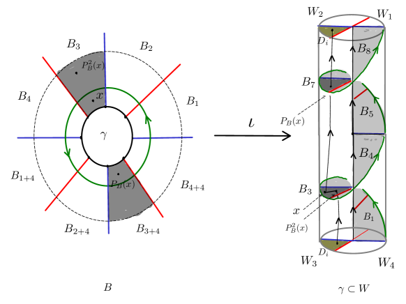
Figure 7: Partition into quadrants of a tame Birkhoff section with $n(\gamma,B)=2$ and $m(\gamma,B)=1$.

Let $D\subset W$ be a local transverse section and $x_{D}$ its intersection point with $\gamma$. Then, the quadrants $W_{1},\dots,W_{4}$ determine four quadrants $D_{i}=D\cap W_{i}$ in $D$. Observe that the first return map $P_{D}:V\to D$ defined in a neighbourhood $V$ of $x_{D}$ preserves the quadrants, i.e. $P_{D}(V\cap D_{i})\subset D_{i}$ for every $i=1,\dots,4$.

Let $B\subset W$ be a tame local Birkhoff section at $\gamma$ with linking number $n$ and multiplicity $m$. Then, because of the tameness hypothesis the four quadrants $W_{i}$ also determine a partition of the annulus $B$ into quadrants. Each of these quadrants can be though of as a rectangle, whose boundary contains a segment of $\gamma$ and two segments which are connected components of $\mathring{B}\cap\left(W^{s}_{loc}(\gamma)\cup W^{u}_{loc}(\gamma)\right)$. Observe that the first return map $P_{B}:\mathring{U}\to\mathring{B}$ defined in a collar neighbourhood $U$ of $\gamma$ sends quadrants of $B$ into quadrant of $B$.

Proposition 3.12 (See [2] or [25]).

There are exactly $4n$ quadrants of $B$, and each $W_{i}$ contains $n$ of them.

If we choose a quadrant of $B$ which lies in $W_{1}$ and we call it $B_{1}$, then we can inductively label the quadrants of $B$ as $B_{1},\dots,B_{4n}$ by declaring that $\forall j=1,\dots,4n$, if $W_{i}$ contains $B_{j}$ then $B_{j+1}$ is the quadrant adjacent to $B_{j}$ which lies in $W_{i+1}$, $i=1,\dots,4$. We will always use this labelling for the quadrants of a Birkhoff section.

3.1.3 Projections along flow lines.

The foliation $\mathcal{O}$ by $\phi_{t}$-orbits of $M$ induces a foliation $\mathcal{O}_{W}$ by orbit segments on the tubular neighbourhood $W$, where for every $x\in W$, $\mathcal{O}_{W}(x)$ is the connected component of $\mathcal{O}(x)\cap W$ that contains $x$. Each segment $\mathcal{O}_{W}(x)$ is parametrized by the action of $\phi_{t}$, that is,

$$\mathcal{O}_{W}(x)=\{\phi_{t}(x):-\infty\leq a_{x}<t<b_{x}\leq+\infty\}$$

for some $a_{x},b_{x}$. The periodic orbit $\gamma$ is the unique $\phi_{t}$-orbit that is entirely contained in $W$.

The (germ of the) $\phi_{t}$-foliation restricted on the tubular neighbourhood $W$ can be obtained by suspending the (germ of the) first return map $P_{D}:V\to D$ onto the transverse disk $D$. On the punctured neighbourhood $W_{\Gamma}\coloneqq W\backslash\gamma$, the foliation by flow orbits can be written as both:

• The suspension of $P_{D}$ on the punctured disk $D^{*}=D\backslash\{x_{D}\}$,

• The suspension of $P_{B}$ on the interior of the Birkhoff section $\mathring{B}=B\backslash\gamma$.

Our aim is to relate this two representations of the foliation induced by $\phi_{t}$-orbits on $W_{\Gamma}$. This can be done by projecting points in $\mathring{B}$, along the flow orbits, onto points in $D^{*}$. Although the surfaces $D^{*}$ and $\mathring{B}$ are not homotopic in $W_{\Gamma}$, these maps can be well-defined over simply connected regions of $\mathring{B}$ (in particular, over the quadrants of the Birkhoff section).

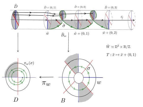
Figure 8: Projection along the flow lines from a local Birkhoff section onto a local transverse section.

Construction.

Let $w$ be a segment which is the closure of a connected component of $\mathring{B}\cap\left(W^{s}_{loc}(\gamma)\right.$ $\left.\cup W^{u}_{loc}(\gamma)\right).$ Since the Birkhoff section is an immersed annulus, we can cut along $w$ and obtain an immersed compact strip inside $W$ (embedded on the interior), with two opposite sides that are naturally identified with $w$. We will denote this strip by $B_{w}$.

Consider a universal cover $\tilde{W}$ of $W$, which is homeomorphic to $\mathbb{D}^{2}\times\mathbb{R}$ since $W\simeq\mathbb{D}^{2}\times\mathbb{R}/\mathbb{Z}$. By lifting the foliation $\mathcal{O}_{W}$ on $W$, we obtain a foliation $\tilde{\mathcal{O}}_{W}$ on $\tilde{W}$ by parametrized segments $\tilde{\phi}_{t}(\tilde{x})$ with $\tilde{x}\in\tilde{W}$ and $-\infty\leq a_{\tilde{x}}<t<b_{\tilde{x}}\leq+\infty$. Let $\tilde{B}_{w}$, $\tilde{D}$ and $\tilde{\gamma}$ be lifts to the universal of $B_{w}$, $D$ and $\gamma$ respectively. By the continuity of the flow there exists some neighbourhood $O$ of the compact segment $\tilde{\gamma}\cap\tilde{B}_{w}$ and some $T>0$ such that, for every $\tilde{x}\in O$, the $\tilde{\phi}_{t}$-segment $[\tilde{\phi}_{-T}(\tilde{x}),\tilde{\phi}_{T}(\tilde{x})]$ intersects the disk $\tilde{D}$ and exactly in one point. This allows to consider a collar neighbourhood $\tilde{U}_{w}$ of $\tilde{\gamma}\cap\tilde{B}_{w}$ inside $O\cap\tilde{B}_{w}$ and to define a map $\tilde{\pi}_{w}:\tilde{U}_{w}\to\tilde{D}$ of the form $\tilde{\pi}_{w}(x)=\tilde{\phi}(s(x),x)$, where $s:\tilde{U}_{w}\to\mathbb{R}$ is continuous, and is bounded as a consequence of the tame hypothesis (cf. [2]). Observe that all the points in $\tilde{\gamma}\cap\tilde{U}_{w}$ are mapped over the intersection point $\tilde{x}_{D}$ of $\tilde{D}$ with $\tilde{\gamma}$, but we will not be interested in these points. So, we will just consider the restriction $\tilde{\pi}_{w}:(\tilde{U}_{w}\backslash\tilde{\gamma})\to(\tilde{D}\backslash\{\tilde{x}_{D}\})$.

Since the universal covering map provides identifications $\tilde{D}\to D$ and $\tilde{B}_{w}\to B_{w}$, we can think of $\tilde{\pi}_{w}$ as a map $\pi_{w}:\mathring{B}_{w}\to D^{*}$ of the form $\pi_{w}(x)=\phi(s(x),x)$, defined for points $x$ in the strip $B_{w}$ which are sufficiently close to $\gamma$.

Definition 3.13.

Let $B$ be a tame local Birkhoff section at $\gamma$, $D$ a local transverse section which intersects $\gamma$ at the point $x_{D}$, and let $w$ be a connected component of $\mathring{B}\cap\left(W^{s}_{loc}(\gamma)\cup W^{u}_{loc}(\gamma)\right)$. A local projection along the flow from $B$ onto $D$ is a map $\pi_{w}:\mathring{U}_{w}\to D^{*}$ of the form $\pi_{w}(x)=\phi(s(x),x)$, where

• $U\subset B$ is a collar neighbourhood of $\gamma$ and $\mathring{U}=U\backslash\gamma$,

• $\mathring{U}_{w}$ is the strip obtained by cutting $\mathring{U}$ along $w$,

• $s:\mathring{U}_{w}\to\mathbb{R}$ is continuous and bounded.

If we choose a quadrant $B_{j}$ of $B$ that lies in $W_{i}$ and we consider the restriction $\pi_{j}=\pi_{w}|_{B_{j}}$, this map is a homeomorphisms between $\mathring{U}\cap B_{j}$ and a open set $V_{i}$ in $D_{i}$ that accumulates in $x_{D}$. The main interest about this map is that it conjugates the first return maps on the quadrant surfaces $B_{j}$ and $D_{i}$. Observe that a projection along the flow depends on the particular choice of the segment $w$, as well as the particular choices of the the lifts of $D$ and $B_{w}$. The following proposition is a summary of different properties relating projections along the flow that appear in [2]. The reader can also encounter a detailed explanation in [25].

Proposition 3.14.

Let $B$ be a tame local Birkhoff section at $\gamma$ with linking number $n\geq 1$ and multiplicity $0\neq m\in\mathbb{Z}$. Let $\pi=\pi_{w}:\mathring{U}_{w}\to D$ be a projection along the flow onto a local transverse section $D$ as defined above. Here, $w$ is a segment of the intersection of $\mathring{B}$ with $W^{s}_{loc}(\gamma)\cup W^{u}_{loc}(\gamma)$. We will enumerate the quadrants of $B$ as $B_{1},\dots,B_{4n}$ in such a way that $B_{1}$ and $B_{4n}$ intersect along $w$. Observe that for all the quadrants $B_{j}$ contained in $W_{i}$ it is satisfied that $j=i+4r$, where $0\leq r\leq n-1$ and $1\leq i\leq 4$. Then, we have that:

1. The map $P_{B}$ permutes cyclically all the quadrants of $B$ that are contained in the same component $W_{i}$, and in particular we have that $P_{B}^{n}$ preserves each quadrant $B_{j}$. Moreover, in the case that $n>1$, let $1\leq k,l\leq n-1$ be such that $k\equiv m$ (mod $n$) and $l\equiv m^{-1}$ (mod $n$). Then, the first return map to $B$ permutes the quadrants in the following fashion:

   1. $P_{B}$ takes the quadrant $B_{j}$ into $\left\{\begin{array}[]{ll}B_{j+4l}&\text{if }m>0,\\ B_{j-4l}&\text{if }m<0.\end{array}\right.$

   2. $P_{B}^{k}$ takes the quadrant $B_{j}$ into $\left\{\begin{array}[]{ll}B_{j+4}&\text{if }m>0,\\ B_{j-4}&\text{if }m<0.\end{array}\right.$

2. Let $B_{j}$ be a quadrant of $B$ where $j=i+4r$, $1\leq i\leq 4$ and $0\leq r\leq n-1$. Let’s denote by $\mathring{U}_{j}=\mathring{U}\cap B_{j}$ and $\pi_{j}$ the restriction $\pi|_{\mathring{U}_{j}}$. Then, the $\pi_{j}$ takes $\mathring{U}_{j}$ homeomorphically onto its image in $D_{i}-\{x_{D}\}$ and it is satisfied that:

   1. The homeomorphism $\pi_{j}$ induces a local conjugacy between $P_{B}^{n}$ and $P_{D}$. That is,

      $$\pi_{j}\circ P_{B}^{n}(z)=P_{D}\circ\pi_{j}(z),\ \forall j=1,\dots,4n\ \text{and}\ z\ \text{sufficiently close to}\ \gamma.$$

   2. The holonomy defect over $w$ is given by

      $$\pi_{1}\circ\pi_{4n}^{-1}(z)=P_{D}^{m}(z),\ \forall\ z\in w=B_{1}\cap B_{4n}\ \text{sufficiently close to}\ \gamma.$$

3. The projection along the flow depends on $w$ and on a particular choice of a lift of $B_{w}$ to the universal cover. For a fix segment $w$ we have that if $\pi_{w}$ and $\pi_{w}^{\prime}$ are two such projections then $\exists$ $k\in\mathbb{Z}$ such that $\pi_{w}^{\prime}=\pi_{w}\circ P_{B}^{k}$, in a suitable common domain of definition.

We provide just an sketch of the proof of proposition 3.14 above, and we refer the reader to [2] or [25] for more accurate details. The proof of this proposition (as well as 3.6 and 3.12 before) resides in the following two claims, explained in the referred works.

First, let $B_{j}$ be a quadrant of $B$ contained in some component $W_{i}$ of $W\backslash(W^{s}_{loc}(\gamma)\cup W^{u}_{loc}(\gamma))$, and let $D_{i}$ be the corresponding quadrant of $D$. Let $\mathring{U}_{j}=\mathring{U}\cap B_{j}$ and $\pi_{j}:\mathring{U}_{j}\to D_{i}$ be the restriction to the quadrant $B_{j}$ of the projection along the flow. The map $\pi_{j}$ is a homeomorphism onto its image. Let’s denote $Q\coloneqq B_{j}$ and let $P_{Q}:\mathring{U}_{j}\to Q$ be the first return map onto the quadrant $Q$. Let $z\in\mathring{U}_{j}$ be a point such that $z^{\prime}=P_{Q}(z)\in\mathring{U}_{j}$, and let $\eta_{0}:[0,1]\to\mathring{U}_{j}$ be an arc contained in $Q$, connecting $\sigma_{0}(0)=z^{\prime}$ with $\sigma_{0}(1)=z$. Define

• $\beta_{0}=[z,z^{\prime}]\cdot\eta_{0}$ is the curve obtained by concatenating the $\phi_{t}$-orbit segment $[z,z^{\prime}]$ with the arc $\eta_{0}$.

• $x=\pi_{j}(z)$, $x^{\prime}=\pi_{j}(z^{\prime})$, $\eta_{1}=\pi_{j}\circ\eta_{0}$. (Observe that $z,\ x,\ z^{\prime},\ x^{\prime}$ all lie in the same $\phi_{t}$-orbit.)

• $\beta_{1}=[x,x^{\prime}]\cdot\eta_{1}$ is the curve obtained by concatenating the $\phi_{t}$-orbit segment $[x,x^{\prime}]$ with the arc $\eta_{1}$.

Claim (1).

If $z$ is chosen sufficiently close to $\gamma$, then $\beta_{0}$ is homotopic to $\beta_{1}$ inside $W_{i}$.

This claim follows from the fact that the formula $\pi_{j}^{\theta}:x\mapsto\phi(\theta s(x),x)$ with $0\leq\theta\leq 1$ defines a proper isotopy between $\pi_{j}$ and the inclusion $Q\hookrightarrow W_{i}$.

Second, since $\mathring{B}\hookrightarrow W\backslash\gamma$ is a properly embedded surface (for a small choice of the regular tubular neighbourhood $W$ of $\gamma$) there is a well-defined notion of algebraic intersection between the homology class $[\alpha]\in H_{1}(W\backslash\gamma)$ of a closed curve $\alpha$ and the relative homology class $[B]\in H_{1}(W,W\cup\gamma)$ of the annulus $\mathring{B}$. This intersection can be defined by counting oriented intersections of a representative $\alpha$ that is transverse to $\mathring{B}$. It is satisfied that:

Claim (2).

Let $\{a,b\}$ be the meridian/longitude basis of $H_{1}(W\backslash\gamma)$ defined in 3.5 above, and let $[\alpha]=p\cdot a+q\cdot b$ be the homology class of a closed curve $\alpha$, where $p,q\in\mathbb{Z}$. Then

$$[\alpha]\cdot[B]=-pm(\gamma,B)+qn(\gamma,B).$$ (3)

Proof of proposition 3.14..

For proving the items in the proposition we have that:

1. Each quadrant $W_{i}$ is homeomorphic to a solid torus, and the map $H_{1}(W_{i})\to H_{1}(W\backslash\gamma)$ induced by the corresponding inclusion sends a generator of $H_{1}(W_{i})$ to the longitude class $b\in H_{1}(W\backslash\gamma)$. The homology class $[\beta_{0}]$ in $H_{1}(W_{i})$ is a generator (since it has intersection number one with the properly embedded disk $Q$) and thus $[\beta_{0}]\cdot[B]=b\cdot[B]$. Since the intersection number $b\cdot[B]$ equals the linking number $n(B,\gamma)$ (cf. [2]), and since $\beta_{0}$ cuts every quadrant $B_{j}$ of $B$ with the same orientation, we conclude that there are $n$ quadrants of $B$ inside $W_{i}$ (proposition 3.12 above) and that $P_{B}$ permutes cyclically these quadrants. Thus, $P_{B}^{n}$ fixes each quadrant $B_{j}$. In addition we have that:

   1. Consider a point $z\in\mathring{B}_{j}$ sufficiently close to $\gamma$ such that $P_{B}^{n}(z)\in\mathring{B}_{j}$. Assume first that $m>0$. Since the orbit segment $[z,P_{B}^{n}(z)]$ intersects once each quadrant inside $W_{i}$ we know that there exists some $1\leq l\leq n-1$ such that $P_{B}(z)\in\mathring{B}_{j+4l}$ and we want to determine $l$. Let $[P_{B}(z),z]$ denote the curve that is obtained by reparametrizing with inverse orientation the orbit segment joining $z$ with $P_{B}(z)$. Consider a curve $\alpha:[0,1]\to B_{j}\cup B_{j+1}\cup\dots\cup B_{j+4l}$ connecting $\alpha(0)=z$ with $\alpha(1)=P_{B}(z)$ and let’s define $\eta$ as the closed path that is obtained by concatenation of $\alpha$ with $[P_{B}(z),z]$.

      Claim (See [25]).

      The homology class of $\eta$ in $H_{1}(N\backslash\gamma)\simeq\mathbb{Z}^{2}$ is $(l,q)$ in the basis given by the meridian and the longitude, where $q$ is some integer.

      Since the segment $[P_{B}(z),z]$ is transverse to $B$ at its endpoints and cuts it with negative orientation, and since $\alpha$ is tangent to $B$, then the homological intersection number satisfies $[B]\cdot[\eta]=-1$. Using that $[B]\cdot[\eta]=-1=-l\cdot m+q\cdot n$ (see claim (2) above) we conclude that $l\equiv m^{-1}$ (mod $n$) when $m>0$. The case $m<0$ is analogous.

   2. The proof of $1(b)$ is similar to the previous one. Assume that $m>0$. We now that there exists some $1\leq k\leq n-1$ such that $P_{B}^{k}(z)\in\mathring{B}_{j+4}$, and we want to determine $k$. Let $[P_{B}^{k}(z),z]$ denote the curve that is obtained by reparametrizing with inverse orientation the orbit segment joining $z$ with $P_{B}^{k}(z)$. Consider a curve $\alpha:[0,1]\to B_{j}\cup B_{j+1}\cup B_{j+2}\cup B_{j+3}\cup B_{j+4}$ connecting $\alpha(0)=z$ with $\alpha(1)=P_{B}^{k}(z)$ and let’s define $\eta$ as the closed path that is obtained as a concatenation of $\alpha$ with $[P_{B}^{k}(z),z]$. It follows that the homology class of $\eta$ in $H_{1}(N\backslash\gamma)$ is $(1,q)$, where $q$ is some integer. Using that $[B]\cdot[\eta]=-k=-m+q\cdot n$ we have that $k\equiv m$ (mod $n$). The case $m<0$ is analogous.

2. Denote $Q=B_{j}$ and consider $z$,$z^{\prime}\in Q$, $x,x^{\prime}\in D_{i}$ and $\beta_{0}$, $\beta_{1}$ defined as in claim (1) above.

   

   Figure 9: Holonomy defect of $\pi_{w}$ along $w$.

   1. Since $z^{\prime}=P_{Q}(z)$ is the first return onto $Q$ then the intersection number $[\beta_{0}]\cdot[Q]$ equals one, and since $Q$ is properly homotopic to $D_{i}$ (inside $W_{i}$) we have also that $[\beta_{1}]\cdot[D_{i}]=1$. Since $\beta_{1}$ is obtained concatenating the oriented orbit segment $[x,x^{\prime}]$ (that always cross $D_{i}$ with the same orientation) and a tangent arc $\eta_{1}$, we conclude that $\beta_{1}$ has only one transverse intersection with $D_{i}$, so $x^{\prime}=P_{D}(x)$. This shows that

      $$\text{For}\ z\ \text{sufficiently close to}\ \gamma\ \Rightarrow\pi_{j}\circ P_{Q}(z)=P_{D}\circ\pi_{j}(z).$$ (4)

      The statement of $2(a)$ follows, since $P_{Q}=P_{B}^{n}$ by item $1$.

   2. To prove $2(b)$, let $\sigma:[0,1]\to\mathring{B}$ be a simple closed curve generating $H_{1}(B)$ such that $\sigma(0)=\sigma(1)=z\in w$ and $\sigma\cap w=\{z\}$. Let $\tilde{\sigma}:[0,1]\to\tilde{B}_{w}$ be a lift to the universal cover. Since $[\sigma]=n\cdot a+m\cdot b$ it follows that $\tilde{\sigma}(1)=T^{m}(\tilde{\sigma}(0))$, where $T:\tilde{W}\to\tilde{W}$ is the generator of the deck transformation group. Hence, the strip $\tilde{B}_{w}$ is delimited by two lifts of $w$, namely $\tilde{w}$ and $T^{m}(\tilde{w})$. Recall that we have defined first a map $\tilde{\pi}_{w}:\tilde{B}_{w}\to\tilde{D}$ (only defined for points near $\tilde{\gamma}$) and then $\pi_{w}:\mathring{B}_{w}\to D^{*}$ by passing to the quotient $\tilde{W}\to W$. By construction we have that

      $$\pi_{4n}(z)=\tilde{\pi}_{w}(\tilde{\sigma}(1))$$ (5)

      $$\pi_{1}(z)=\tilde{\pi}_{w}(\tilde{\sigma}(0)).$$ (6)

      Let $\psi:T^{m}(\tilde{w})\to\tilde{w}$ be the projection along the flow lines in the universal cover, so that

      $$\tilde{\pi}_{w}|_{T^{m}(\tilde{w})}=\tilde{\pi}_{w}|_{\tilde{w}}\circ\psi.$$

      Recall that $w$ is a segment contained in $B\cap\left(W^{s}_{loc}(\gamma)\cup W^{u}_{loc}(\gamma)\right)$ and transverse to the flow, so there is a first return map $P_{w}:w\to w$ and $\pi_{1}\circ P_{w}=P_{D}\circ\pi_{1}$ as in (4) above. Since $m>0$, the map $\psi$ from $T^{m}(\tilde{w})$ to $\tilde{w}$ on the universal cover induces the $-m$-th power of $P_{w}$ on the segment $w$. We can conclude that

      $$\pi_{4n}(z)=\pi_{1}\circ P_{w}^{-m}(z)=P_{D}^{-m}\circ\pi_{1}(z).$$

3. Fix the segment $w$ in $B\cap(W^{s}_{loc}(\gamma)\cup W^{u}_{loc}(\gamma))$ and chose flow projections $\pi_{w}$ and $\pi_{w}^{\prime}$ from $B_{w}$ onto a transverse section $D$. Denote by $\tilde{D}$, $\tilde{B}_{w}$ and $\tilde{D}^{\prime}$, $\tilde{B}_{w}^{\prime}$ the corresponding lifts of $D$ and $B_{w}$ used to define $\pi_{w}$ and $\pi_{w}^{\prime}$, respectively. By the continuity of the flow, we can define projections along the flow lines $\psi_{D}:\tilde{D}\to\tilde{D}^{\prime}$ and $\psi_{B}:\tilde{B}_{w}^{\prime}\to\tilde{B}_{w}$ (in suitable neighbourhoods of $\tilde{\gamma}$) so that $\tilde{\pi}_{w}^{\prime}=\psi_{D}\circ\tilde{\pi}_{w}\circ\psi_{B}$. These projections induce on the quotient return maps $P_{D}^{r}:D\to D$ and $P_{B}^{l}:\mathring{B}\to\mathring{B}$, where $r,l$ are integers such that $\tilde{D}^{\prime}=T^{r}(\tilde{D})$ and $\tilde{B}_{w}=T^{l}(\tilde{B}_{w}^{\prime})$. Hence, using $2(a)$ we conclude that

   $$\pi_{w}^{\prime}=P_{D}^{r}\circ\pi_{w}\circ P_{B}^{l}=\pi_{w}\circ P_{B}^{k},\ \text{where}\ k=nr+l.$$

∎

3.1.4 Deformation by flow isotopies, equivalence and existence of tame Birkhoff sections.

Given two embedded transverse sections of a non-singular flow, the natural way to relate these surfaces together with its first return maps (if defined) is via flow-isotopies, which are homeomorphisms between the surfaces obtained by pushing along flow lines. We explain this for the case of local Birkhoff sections.

Let $\phi_{t}:M\to M$ be a non-singular regular flow having a saddle type periodic orbit $\gamma$ with orientable invariant manifolds.

Definition 3.15.

Two local Birkhoff sections $B$ and $B^{\prime}$ at $\gamma$ are $\phi_{t}$-isotopic if there exist collar neighbourhoods $U\subset B$ and $U^{\prime}\subset B^{\prime}$ of $\gamma$ and a continuous and bounded function $s:\mathring{U}\to\mathbb{R}$, such that the map $\psi$ given by $\psi(x)=\phi(s(x),x)$, $x\in\mathring{U}$, defines a homeomorphism between $\mathring{U}$ and $\mathring{U}^{\prime}$. (Recall the notation $\mathring{U}=U\backslash\gamma$.)

Proposition 3.16 (See [25]).

Let $B$ and $B^{\prime}$ be two local Birkhoff sections at $\gamma$ which are $\phi_{t}$-isotopic, and let $\psi:\mathring{U}\to\mathring{U}^{\prime}$ be a $\phi_{t}$-isotopy. Let’s also assume that the first return map $P_{B}$ is defined for every point in $\mathring{U}$. Then:

1. Up to shrinking the neighbourhoods $U$ and $U^{\prime}$ if necessary, it is satisfied that $\psi\circ P_{B}(x)=P_{B^{\prime}}\circ\psi(x)$, for every $x\in\mathring{U}$;

2. If $\psi^{\prime}$ is another $\phi_{t}$-isotopy then $\exists$ $N\in\mathbb{Z}$ such that $\psi^{\prime}(x)=\psi\circ P_{B}^{N}(x)$, for every $x\in\mathring{U}$ sufficiently close to $\gamma$.

If $B$ and $B^{\prime}$ are $\phi_{t}$-isotopic it follows that they have the same linking numbers and multiplicities. Conversely, it is satisfied that

Proposition 3.17 (See [2]).

Let $B$ and $B^{\prime}$ be two tame local Birkhoff sections on a saddle type periodic orbit $\gamma$. Then $B$ is $\phi_{t}$-isotopic to $B^{\prime}$ if and only if $n(\gamma,B)=n(\gamma,B^{\prime})$ and $m(\gamma,B)=m(\gamma,B^{\prime})$.

In [2] the proof is done just for the case when $m(\gamma,B)=m(\gamma,B^{\prime})=1$, but it can be adapted to the general setting. Observe that a $\phi_{t}$-isotopy is defined by pushing along flow lines with a continuous and bounded function $s:\mathring{U}\to\mathbb{R}$. To obtain a bounded function it is essential the hypothesis of tameness.

The following proposition will be used for the proof of theorem 3.9. It states that given two $\phi_{t}$-isotopic local Birkhoff sections $B$ and $B^{\prime}$ at $\gamma$, it is possible to interpolate them to create a new local Birkhoff section that coincides with $B^{\prime}$ near $\gamma$ and with $B$ outside a neighbourhood of $\gamma$.

Proposition 3.18 (See [2]).

Let $B$ and $B^{\prime}$ be two local Birkhoff sections on a saddle type periodic orbit $\gamma$, with the same linking number and multiplicity. Then, there exists a neighbourhood $W$ of $\gamma$ such that: For any neighbourhood $O\subset W$ there exist another neighbourhood $O^{\prime}\subset O$ and a continuous and bounded function $s:W\backslash\gamma\to\mathbb{R}$ such that the map $\psi(u)=\phi(s(u),u)$ defines an $\phi_{t}$-isotopy onto its image, and

1. $\psi(u)\in\mathring{B}^{\prime}$, for all $u\in\mathring{B}\cap O^{\prime}$,

2. $\psi(u)=u$, for all $u\in\mathring{B}\cap W\backslash O$.

Concerning the tameness condition defined at the beginning, general (local) Birkhoff sections need not to be tame. It is possible to construct smoothly embedded local Birkhoff sections in a neighbourhood of a periodic orbit $\gamma$ that intersect $W^{s}_{loc}(\gamma)$ or $W^{u}_{loc}(\gamma)$ in a very narrow way, for example, along an infinite curve accumulating over an interval $I\subset\gamma$ non reduced to a singleton. Nevertheless, the previous proposition can be used to modify any given Birkhoff section in a neighbourhood of the boundary components and obtain a tame one. (Observe that tameness is not demanded in the hypothesis of proposition 3.18.)

Proposition 3.19 (See [2]).

Let $\phi_{t}:M\to M$ be a non-singular flow on a closed $3$-manifold and let $\iota:(\Sigma,\partial\Sigma)\to(M,\Gamma)$ be a Birkhoff section, such that every $\gamma\in\Gamma$ is a saddle type periodic orbit. Then, given a neighbourhood $W$ of $\Gamma$ (that one can think of as a finite union of tubular neighbourhoods around each curve in $\Gamma$) there exists a Birkhoff section $\iota^{\prime}:(\Sigma,\partial\Sigma)\to(M,\Gamma)$, with image $\Sigma^{\prime}=\iota^{\prime}(\Sigma)$, satisfying that:

1. $\mathring{\Sigma}\cap(M\backslash W)\equiv\mathring{\Sigma}^{\prime}\cap(M\backslash W)$,

2. $\Sigma^{\prime}$ is tame at each boundary curve $\gamma\in\Gamma$.

3.2 Local version of theorem 3.9.

For $i=1,2$ consider a topological saddle type periodic orbit $\gamma^{i}$ of a flow $\phi_{t}^{i}:M_{i}\to M_{i}$ such that their local stable and unstable manifolds are orientable. Let $B_{i}\hookrightarrow M_{i}$ be a tame local Birkhoff section at $\gamma^{i}$, and assume that there exists a local conjugation $h:(B_{1},P_{B_{1}})_{\gamma^{1}}\to(B_{2},P_{B_{2}})_{\gamma^{2}}$ between the first return maps $P_{B_{i}}$.

Let’s recall that $h:\mathring{B}_{1}\to\mathring{B}_{2}$ is a homeomorphism, where $\mathring{B}_{i}=B\backslash\gamma^{i}$, such that $P_{B_{2}}\circ h(x)=h\circ P_{B_{1}}(x)$, for every $x\in\mathring{B}_{1}$ sufficiently close to $\gamma^{1}$.

By lemma 2.6, we have that for every sufficiently small neighbourhood $W_{1}$ of $\gamma^{1}$, the homeomorphism $h$ induces a homeomorphism $H:W_{1}\backslash\gamma^{1}\to W_{2}\backslash\gamma^{2},$ where $W_{2}$ is a neighbourhood of $\gamma^{2}$, which is a local orbital equivalence $(\phi_{t}^{1},W_{1}\backslash\gamma_{1})\to(\phi_{t}^{1},W_{1}\backslash\gamma_{1})$ in the sense of definition 2.2, and whose restriction onto $\mathring{B}_{1}\cap W_{1}$ coincides with $h$.

Theorem 3.20.

Consider a homeomorphism $H:W_{1}\backslash\gamma^{1}\to W_{2}\backslash\gamma^{2}$, where $W_{1}$ and $W_{2}$ are neighbourhoods of $\gamma^{1}$ and $\gamma^{2}$ respectively, which verifies that

1. $H:(\phi_{t}^{1},W_{1}\backslash\gamma^{1})\to(\phi_{t}^{2},W_{2}\backslash\gamma^{2})$ is an orbital equivalence,

2. $H(x)=h(x)$ for every $x\in\mathring{B}_{1}\cap W_{1}$.

If it is satisfied that $m(\gamma^{1},B_{1})=m(\gamma^{2},B_{2})\text{ and }n(\gamma^{1},B_{1})=n(\gamma^{2},B_{2})$, then for every neighbourhood $N\subset W_{1}$ there exists a homeomorphisms $H_{N}:W_{1}\to W_{2}$ such that:

1. $H_{N}$ is a local orbital equivalence between $(\phi_{t}^{1},W_{1})_{\gamma^{1}}$ and $(\phi_{t}^{2},W_{2})_{\gamma^{2}}$,

2. $H_{N}(x)=H(x)$, for every $x\in W_{1}\backslash N$.

Remark 3.21.

An orbital equivalence $H:(\phi_{t}^{1},W_{1}\backslash\gamma^{1})\to(\phi_{t}^{2},W_{2}\backslash\gamma^{2})$ that coincides with $h$ over the Birkhoff sections $B_{i}$ does not extend to a homeomorphism between $W_{1}$ and $W_{2}$, in general. This is because, in general, the homeomorphism $h:\mathring{B}_{1}\to\mathring{B}_{2}$ does not extend to the boundary. (cf. 4.)

To prove theorem 3.20 we will show that given some neighbourhood $N\subset W_{1}$ of $\gamma^{1}$, under the assumption that the sections are tame, it is possible to modify $H$ inside this neighbourhood by pushing along flow lines, and obtain a new homeomorphism $H_{N}$ that extends as an orbital equivalence over the whole sets $W_{i}$.

3.2.1 Proof of theorem 3.20.

Consider an orbital equivalence

$$H:(\phi_{t}^{1},W_{1}\backslash\gamma^{1})\to(\phi_{t}^{2},W_{2}\backslash\gamma^{2})$$ (7)

such that its restriction to the interior of the Birkhoff section $B_{1}$ coincides with $h:\mathring{B}_{1}\to\mathring{B}_{2}$, as in the hypothesis of 3.20. Observe that if we replace the neighbourhoods $W_{i}$ by smaller neighbourhoods $W_{i}^{\prime}\subset W_{i}$, then it is enough to prove the theorem for these new neighbourhoods. We will shrink the size of the $W_{i}$ several times in the course of the proof. Theorem 3.20 relies in the following proposition.

Proposition 3.22.

For $i=1,2$ consider a saddle type periodic orbit $\gamma^{i}$ of a flow $\phi_{t}^{i}:M_{i}\to M_{i}$ such that their local stable and unstable manifolds are orientable. Consider:

• $B_{i}$ a tame local Birkhoff section at $\gamma^{i}$ and assume that there exists a local conjugation $h:(B_{1},P_{B_{1}})_{\gamma^{1}}\to(B_{2},P_{B_{2}})_{\gamma^{2}}$ between the first return maps $P_{B_{i}}$,

• For each orbit $\gamma^{i}$ let $D_{i}$ be a local transverse section. Let $x^{i}=\gamma^{i}\cap D_{i}$ and let $\pi^{i}:(\mathring{B}_{i})_{w_{i}}\to D_{i}\backslash\{x^{i}\}$ be projections along the flow as defined in 3.13 above, where $w_{i}$ is a fixed segment of the intersection of $B_{i}$ with the local invariant manifolds of $\gamma^{i}$.

If it is satisfied that $m(\gamma^{1},B_{1})=m(\gamma^{2},B_{2})\text{ and }(\gamma^{1},B_{1})=n(\gamma^{2},B_{2})$, then there exists a homeomorphism $h_{D}:D_{1}\to D_{2}$ satisfying that:

1. $h_{D}$ is a local conjugation between $(D_{1},P_{D_{1}})_{x^{1}}$ and $(D_{2},P_{D_{2}})_{x^{2}}$,

2. $\exists$ a collar neighbourhood $U_{1}\subset B_{1}$ of the curve $\gamma^{1}$ such that $h_{D}\circ\pi^{1}(x)=\pi^{2}\circ h(x)$, $\forall\ x\in U_{1}$.

We postpone the proof of this proposition to the end. Now, with this result we can deduce theorem 3.20 in the following way: For each orbit $\gamma^{i}$ consider a local transverse section $D_{i}$ and a projection along the flow $\pi^{i}:(\mathring{B}_{i})_{w_{i}}\to D_{i}\backslash\{x_{i}\}$ as the previous proposition. Since we assume in the hypothesis of theorem 3.20 that linking number and multiplicities coincide for both $B$ and $B^{\prime}$, we can apply proposition 3.22 and obtain a homeomorphism $h_{D}:D_{1}^{\prime}\to D_{2}^{\prime}$ satisfying $(a)$ and $(b)$, where $D_{i}^{\prime}\subset D_{i}$ are smaller transverse sections. Using proposition 2.7 we see that there exist a tubular neighbourhood $W_{i}^{\prime}$ of each $\gamma^{i}$ and a local orbital equivalence

$$H_{D}:(\phi_{t}^{1},W_{1}^{\prime})_{\gamma^{1}}\to(\phi_{t}^{2},W_{2}^{\prime})_{\gamma^{2}}$$ (8)

such that $H_{D}(x)=h_{D}(x)$, for every $x\in D_{1}^{\prime}\cap W_{1}^{\prime}$. Without loss of generality we can assume that $W_{1}=W_{1}^{\prime}$. That is, we can assume that the two homeomorphisms $H$ and $H_{D}$ have the same domain.

Theorem 3.20 follows directly from the following proposition.

Proposition 3.23.

For every neighbourhood $N\subset W_{1}$ of $\gamma^{1}$ there exists another neighbourhood $N^{\prime}\subset N$ and a local orbital equivalence $H_{N}:(\phi_{t}^{1},W_{1})_{\gamma^{1}}$ $\to(\phi_{t}^{2},W_{2})_{\gamma^{2}}$ such that:

1. $H_{N}(x)=H(x)$ for every $x\in W_{1}\backslash N$,

2. $H_{N}(x)=H_{D}(x)$, for every $x\in N^{\prime}$.

We dedicate the rest of this part to prove 3.23 and 3.22.

3.2.2 Proof of proposition 3.23.

We start by writing a scheme of the steps in the proof, and then we show each step.

Scheme of the proof.

Consider a neighbourhood $N\subset W_{1}$. Let’s denote $N_{1}=N$.

Step 1

For every neighbourhood $O_{1}\subset W_{1}$ of $\gamma^{1}$ we can find a smaller neighbourhood $O_{1}^{\prime}\subset O_{1}$ and an orbital equivalence $F:(\phi_{t}^{1},W_{1}\backslash\gamma^{1})\to(\phi_{t}^{2},W_{2}\backslash\gamma^{2})$ such that:

1. $F(x)=H(x)$ for every $x\in B_{1}\cap(W_{1}\backslash O_{1})$,

2. $F(x)=H_{D}(x)$ for every $x\in\mathring{B}_{1}\cap O_{1}^{\prime}$.

Step 2

We will find a collection of neighbourhoods

• $N_{1}^{\prime}\subset O_{1}^{\prime}\subset O_{1}\subset N_{1}\subset W_{1},$

• $N_{2}^{\prime}\subset O_{2}^{\prime}\subset O_{2}\subset N_{2}\subset W_{2}.$

Let’s define $V_{i}=N_{i}\backslash O_{i}$ and $V_{i}^{\prime}=O_{i}^{\prime}\backslash N_{i}^{\prime}$. If these neighbourhoods are suitably chosen, we will be able:

• to make an interpolation along the flow lines between $H$ and $F$ supported in the region $V_{1}$, and obtain an orbital equivalence $H_{V}:(\phi_{t}^{1},V_{1})$ $\to(\phi_{t}^{2},V_{2})$ satisfying that:

  1. $H_{V}(x)=H(x)$ for every $x\in\partial N_{1}$,

  2. $H_{V}(x)=F(x)$ for every $x\in\partial O_{1}$;

• to make an interpolation along the flow lines between $H_{D}$ and $F$ supported in the region $V_{1}^{\prime}$, and obtain an orbital equivalence $H_{V}^{\prime}:(\phi_{t}^{1},V_{1}^{\prime})\to(\phi_{t}^{2},V_{2}^{\prime})$ satisfying that:

  1. $H_{V}^{\prime}(x)=F(x)$ for every $x\in\partial O_{1}^{\prime}$,

  2. $H_{V}^{\prime}(x)=H_{D}(x)$ for every $x\in\partial N_{1}^{\prime}$.

Step 3

We will define $H_{N}$ in the following way:

$$H_{N}(x)=\left\{\begin{array}[]{lcc}H(x)&\text{if}&x\in W_{1}\backslash N_{1},\\ \\ H_{V}(x)&\text{if}&x\in N_{1}\backslash O_{1},\\ \\ F(x)&\text{if}&x\in O_{1}\backslash O_{1}^{\prime},\\ \\ H_{V}^{\prime}(x)&\text{if}&x\in O_{1}^{\prime}\backslash N_{1}^{\prime},\\ \\ H_{D}(x)&\text{if}&x\in N_{1}^{\prime}.\\ \end{array}\right.$$ (9)

Observe that $H_{N}$ is well defined in all the boundaries $\partial N_{1}^{\prime}$, $\partial O_{1}^{\prime}$, $\partial O_{1}$, $\partial N_{1}$ and gives rise to a local orbital equivalence satisfying the conclusion of 3.23.

Step 1: The construction of $F$

Lemma 3.24.

Let $O_{1}\subset W_{1}$ be a tubular neighbourhood of $\gamma^{1}$. Then, there exists another tubular neighbourhood $O_{1}^{\prime}\varsubsetneq O_{1}$ and a homeomorphism $F:W_{1}\backslash\gamma^{1}\to W_{2}\backslash\gamma^{2}$ satisfying that:

1. $F:(\phi_{t}^{1},W_{1}\backslash\gamma^{1})\to(\phi_{t}^{2},W_{2}\backslash\gamma^{2})$ is an orbital equivalence,

2. $F(x)=H(x)$ for every $x\in B_{1}\backslash O_{1}$,

3. $F(x)=H_{D}(x)$ for every $x\in\mathring{B}_{1}\cap O_{1}^{\prime}$.

Let’s define

$$S\coloneqq\left\{H_{D}(x):x\in B_{1}\cap W_{1}\right\}.$$ (10)

Then $S$ is a local Birkhoff section at $\gamma^{2}$. Observe in addition that $S$ satisfies that $m(\gamma^{1},S)=m(\gamma^{2},B_{2})$ and $n(\gamma^{1},S)=n(\gamma^{2},B_{2}).$ Following proposition 3.17 we see that $B_{2}$ and $S$ are $\phi_{t}^{2}$-isotopic. Our next goal is to deform $B_{2}$ pushing along flow lines and obtain a new local Birkhoff section $B_{2}^{\prime}$, that coincides with $B_{2}$ outside a tubular neighbourhood $O_{2}$ of the orbit $\gamma^{2}$ and coincides with $S$ in a smaller neighbourhood $O_{2}^{\prime}\subset O_{2}$.

Lemma 3.25.

Let $O_{2}\subset W_{2}$ be a neighbourhood of $\gamma^{2}$. Then, there exist a smaller neighbourhood $O_{2}^{\prime}\subset O_{2}$, a local Birkhoff section $B_{2}^{\prime}$ at $\gamma^{2}$ and a homeomorphism $\psi:\mathring{B}_{2}\to\mathring{B}_{2}^{\prime}$ such that

1. $B_{2}^{\prime}\backslash O_{2}\equiv B_{2}\backslash O_{2}$ and $B_{2}^{\prime}\cap O_{2}^{\prime}\equiv S\cap O_{2}^{\prime}$,

2. $\psi$ is an isotopy along the $\phi_{t}^{2}$-orbits and satisfies that $\psi(y)=y$, $\forall$ $y\in B_{2}\backslash O_{2}$,

3. if $x\in\mathring{B}_{1}$ satisfies that $h(x)\in B_{2}\cap O_{2}^{\prime}$ then $\psi(h(x))=H_{D}(x)$.

Proof.

As usual we will denote $\mathring{S}=S\backslash\gamma^{2}$. Let’s start by constructing a $\phi_{t}^{2}$-isotopy from $\mathring{B}_{2}$ to $\mathring{S}$. By proposition 3.17 there exists a collar neighbourhood $U_{2}\subset B_{2}$ of the curve $\gamma^{2}$ and a continuous and bounded function $s:\mathring{U}_{2}\to\mathbb{R}$ such that the map

$$\varphi:\mathring{U}_{2}\to\mathring{S}\backslash\gamma^{2}\text{ defined by }\varphi(y)=\phi^{2}(y,s(y))$$ (11)

is a $\phi_{t}^{2}$-isotopy from $\mathring{U}_{2}$ into $\mathring{S}$.

Consider $U_{1}=h^{-1}(U_{2})\subset B_{1}$. We will chose the neighbourhoods $U_{i}$ sufficiently small, such that they are contained in the domain of definition of the projections $\pi^{i}:(B_{i})_{\gamma^{i}}\to(D_{i})_{x^{i}}$. Let $P_{S}$ be the first return to the local Birkhoff section $S$.

Lemma 3.26.

There exists $k\in\mathbb{Z}$ such that $\varphi(h(x))=P_{S}^{k}\circ H_{D}(x)$, for every $x\in\mathring{U}_{1}$.

We postpone the proof of this lemma to the end. As a consequence this lemma, up to shrinking the size of $U_{i}$ if necessary and composing with some power of $P_{S}$ on the left, we can assume that $\varphi(h(x))=H_{D}(x)$ for every $x\in\mathring{U}_{1}$.

Given a neighbourhood $O_{2}\subset W_{2}$ of $\gamma^{2}$, we can use proposition 3.18 and find another neighbourhood $O_{2}^{\prime}\subset O_{2}$ and a continuous and bounded function $s^{\prime}:\mathring{B}_{2}\to\mathbb{R}$, such that the map

$$\psi:y\mapsto\phi^{2}(y,s^{\prime}(y)),\ y\in\mathring{B}_{2}$$ (12)

satisfies the following

1. The image $B_{2}^{\prime}\coloneqq\psi(B_{2})$ is a local Birkhoff section and $\psi:\mathring{B}_{2}\to\mathring{B}_{2}^{\prime}$ is a flow isotopy,

2. $\psi(y)=y$ for every $y\in B_{2}\backslash O_{2}$,

3. $\psi(y)=\varphi(y)$ for every $y\in\mathring{B}_{2}\cap O_{2}^{\prime}$.

The neighbourhood $O_{2}^{\prime}$, the section $B_{2}^{\prime}$ and the map $\psi$ satisfy the properties claimed in lemma 3.26. To complete the proof it rest to prove 3.26.

Proof of lemma 3.26.

Recall that the homeomorphism $h_{D}$ satisfies properties $(a)$ and $(b)$ of 3.22 and that $H_{D}$ coincides with $h_{D}$ over the transverse section $D_{1}\cap W_{1}$. Recall also that for every point $z\in W_{i}$ we denote the connected component of $\mathcal{O}^{i}(z)\cap W_{i}$ that contains $z$ as $\mathcal{O}^{i}_{W_{i}}(z)$. We claim that if $x\in\mathring{U}_{1}$ then $\mathcal{O}^{2}_{W_{2}}(H_{D}(x))$ coincides with $\mathcal{O}^{2}_{W_{2}}(h(x))$. Since the projections along the flow preserve orbit segments, it is satisfied that

$$\mathcal{O}^{i}_{W_{i}}(z)=\mathcal{O}^{i}_{W_{i}}(\pi^{i}(z)),\ \forall z\in\mathring{U}_{i}.$$

So we have that

$$\mathcal{O}^{2}_{W_{2}}(H_{D}(x))=H_{D}(\mathcal{O}^{1}_{W_{1}}(x))=H_{D}(\mathcal{O}^{1}_{W_{1}}(\pi^{1}(x)))=\mathcal{O}^{2}_{W_{2}}(H_{D}\circ\pi^{1}(x)).$$

Since $H_{D}\circ\pi^{1}(x)=h_{D}\circ\pi^{1}(x)$ and by 3.22-$(b)$, the last term of the previous equality is equal to

$$\mathcal{O}^{2}_{W_{2}}(h_{D}\circ\pi^{1}(x))=\mathcal{O}^{2}_{W_{2}}(\pi^{2}\circ h(x))=\mathcal{O}^{2}_{W_{2}}(h(x)),$$

so the claim follows. Now, since $\varphi(h(x))$ is a point in $\mathring{S}$ whose orbit segment inside $W_{2}$ equals that of $H_{D}(x)$ we deduce that $\varphi(h(x))=P_{S}^{k}\circ H_{D}(x)$ for some $k\in\mathbb{Z}$. By the continuity of the flow this integer must vary continuously with respect to $x$, so it is constant. This completes the lemma. ∎

∎

As a corollary of 3.25 we have the proof of 3.24.

Proof of 3.24.

Let $V\subset B_{1}$ be a collar neighbourhood of $\gamma^{1}$ contained in the domain of definition of the first return map $P_{B_{1}}$. Let $\mathcal{V}$ be the union of all the compact orbit segments connecting each point in $V$ with its first return to $B_{1}$. Up to shrinking the size of the neighbourhoods $W_{i}$ if necessary, we can assume that $W_{1}\subset\textsl{int}(\mathcal{V})$.

Given $O_{1}\subset W_{1}$ consider $O_{2}=H(O_{1})$. Then, 3.25 gives another neighbourhood $O_{2}^{\prime}\subset O_{2}$, a section $B_{2}^{\prime}$ and a $\phi_{t}^{2}$-isotopy $\psi:\mathring{B}_{2}\to\mathring{B}_{2}^{\prime}$. Let’s define $O_{1}^{\prime}=H_{D}^{-1}(O_{2}^{\prime})$ and $h^{\prime}:\mathring{B}_{1}\to\mathring{B}_{2}^{\prime}$ given by $h^{\prime}(x)=\psi\circ h(x)$. Then, the homeomorphism $h^{\prime}$ is a local conjugation between the first return maps to the Birkhoff sections $B_{1}$ and $B_{2}^{\prime}$ respectively. So it induces an orbital equivalence $F$ with domain $\mathcal{V}\backslash\gamma^{1}$ that coincides with $h^{\prime}$ over $\mathring{B}_{1}\cap\mathcal{V}$. Since $W_{1}\subset\textsl{int}(\mathcal{V})$ we can consider its restriction to $W_{1}\backslash\gamma^{2}$, that is $F:W_{1}\backslash\gamma^{1}\to W_{2}\backslash\gamma^{2}$. It is direct that $F$ coincides with $H$ over $B_{1}\backslash O_{1}$ and with $H_{D}$ over $\mathring{B}_{1}\cap O_{1}^{\prime}$. ∎

Step 2: The interpolation

We start by describing how to choose the neighbourhoods $N_{i}^{\prime}\subset O_{i}^{\prime}\subset O_{i}\subset N_{i}$. Given a regular tubular neighbourhood $O_{1}\subset N_{1}$ of $\gamma^{1}$ consider the annulus $A=B_{1}\cap N_{1}\backslash O_{1}$. We claim that if $O_{1}$ is sufficiently small, then there exists a compact annulus $K$ with non empty interior and contained in $\textsl{int}(A)$, such that $P_{B_{1}}(K)\subset\textsl{int}(A)$. The claim follows directly by examining the first return map in $\mathring{B}_{1}$.

A tubular neighbourhood is said to be regular if its closure is a submanifold homeomorphic to a compact disk times an interval. Given $N_{1}=N$ we will chose a family of regular tubular neighbourhoods $N_{1}^{\prime}\subset O_{1}^{\prime}\subset O_{1}\subset N_{1}$ in the following way:

1. Choose $O_{1}\subset N_{1}$ such that there exists a compact annulus $K$ with non-empty interior contained in $A_{1}=B_{1}\cap N_{1}\backslash O_{1}$, which satisfies that $P_{B_{1}}(K)\subset\textsl{int}(A_{1})$,

2. Choose $O_{1}^{\prime}\subset O_{1}$ given by 3.24,

3. Choose $N_{1}^{\prime}\subset O_{1}^{\prime}$ such that there exists a compact annulus $K^{\prime}$ with non-empty interior contained in $A_{1}^{\prime}=B_{1}\cap O_{1}^{\prime}\backslash N_{1}^{\prime}$, which satisfies that $P_{B_{1}}(K^{\prime})\subset\textsl{int}(A_{1}^{\prime})$.

Let $F:W_{1}\backslash\gamma^{1}\to W_{2}\backslash\gamma^{2}$ given by 3.24 for the chosen neighbourhood $O_{1}$. We will define as well:

1. $N_{2}=H(N_{1})$,

2. $O_{2}=F(O_{1})$ and $O_{2}^{\prime}=F(O_{1}^{\prime})$,

3. $N_{2}^{\prime}=H_{D}(N_{1}^{\prime})$.

Let’s define $V_{i}=\bar{N}_{i}\backslash\textsl{int}(O_{i})\subset M_{i}$ and $V_{i}^{\prime}=\bar{O}_{i}^{\prime}\backslash\textsl{int}(N_{i}^{\prime})\subset M_{i}$. Since the neighbourhoods that we consider are regular tubular neighbourhoods it follows that $V_{i}$ and $V_{i}^{\prime}$ are homeomorphic to a closed annulus times a circle. The topological equivalence $H_{N}$ will be an interpolation between $H$ and $F$ over the set $V_{1}$ and between $H_{D}$ and $F$ over the set $V_{1}^{\prime}$. We describe first the topology of these interpolating sets and then we indicate how to make these interpolations over $V_{1}$ and $V_{2}$.

The Interpolating Neighbourhoods.

Consider the compact sets

$$V_{i}=\bar{N}_{i}\backslash\textsl{int}(O_{i})\subset M_{i}$$ (13)

$$V_{i}^{\prime}=\bar{O}_{i}^{\prime}\backslash\textsl{int}(N_{i}^{\prime})\subset M_{i}.$$ (14)

From now on we will concentrate just in $V_{i}$, $i=1,2$, since all the arguments will be analogous for $V_{i}^{\prime}$. The boundary components of each $V_{i}$ are $\partial N_{i}$ and $\partial O_{i}$. The compact annulus $A_{i}=B_{i}\cap V_{i}$ is a properly embedded surface in $V_{i}$. Consider the compact annuli with non empty interior $K_{1}=K\subset\textsl{int}(A_{1})$ and $K_{2}=h(K)\subset\textsl{int}(A_{2})$. Each $K_{i}$ divides $A_{i}$ into three annuli as in figure 10. We will name the boundaries of $K_{i}$ as $\alpha_{i}$ and $\beta_{i}$ according to this figure. The map $h$ restricts to a homeomorphism $h:A_{1}\to A_{2}$ which defines a conjugacy between the return maps $P_{K_{i}}:K_{i}\to A_{i}$.

Figure 10: The sets $V_{i}$ and the annuli $A_{i}$.

Consider the set

$$\mathcal{K}_{i}=\{\phi_{t}^{i}(u):u\in K_{i},0\leq t\leq\tau^{i}(u)\}$$ (15)

where $\tau^{i}(u)$ is the time of the first return to $B_{i}$ of a point $u\in K_{i}$. This set is the union of all the compact orbit segments joining a point $u\in K_{i}$ with its first return $P_{K_{i}}(u)=\phi^{i}(u,\tau^{i}(u))$. Observe that these orbit segments are disjoint from the boundary components of $V_{i}$ so it is satisfied that $\mathcal{K}_{i}\subset\textsl{int}(V_{i})$. Since we have that $H{|}_{K_{1}}=F{|}_{K_{1}}=h{|}_{K_{1}}$ then it is verified that $\mathcal{K}_{2}=H(\mathcal{K}_{1})=F(\mathcal{K}_{1})$.

The annulus $A_{i}$ is an essential surface in $V_{i}$ and the complement of $\mathcal{K}_{i}\cup A_{i}$ has two connected components. We will call $\mathcal{C}_{i}\text{ and }\mathcal{D}_{i}$ to the closure of these components, where the first one is the component that contains $\partial N_{i}$ in its boundary and the second one is the one that contains $\partial O_{i}$ in its boundary. So, we have a decomposition

$$V_{i}=\mathcal{C}_{i}\cup\mathcal{K}_{i}\cup\mathcal{D}_{i}$$

of the neighbourhood $V_{i}$ into three closed sets.

If we cut the set $V_{i}$ along $A_{i}$ we obtain a manifold $\widetilde{V}_{i}$ homeomorphic to the product of $A_{i}$ with a closed interval that we have depicted in figure 11. This manifold is equipped with a map $\widetilde{V}_{i}\to V_{i}$ which corresponds to glue back the two copies of $A_{i}$. The three sets $\mathcal{C}_{i}$, $\mathcal{K}_{i}$ and $\mathcal{D}_{i}$ lift into $\widetilde{V}_{i}$ and gives a decomposition

$$\widetilde{V}_{i}=\widetilde{\mathcal{C}}_{i}\cup\widetilde{\mathcal{K}}_{i}\cup\widetilde{\mathcal{D}}_{i}$$

into three compact sets, each one homeomorphic to an annulus times an interval. The components $\widetilde{\mathcal{C}}_{i}$ and $\widetilde{\mathcal{D}}_{i}$ are disjoint, and they intersect $\widetilde{\mathcal{K}}_{i}$ along the annuli $L_{\alpha_{i}}$ and $L_{\beta_{i}}$ respectively, as in figure 11.

Observe that the foliation by orbit segments in $V_{i}$ lift into a foliation by segments in $\widetilde{V}_{i}$ which are transverse to the copies of $A_{i}$. Let’s denote by $\widetilde{A}_{i}^{0}$ to the copy of $A_{i}$ where the lifted orbits point inward the manifold $\widetilde{V}_{i}$ and by $\widetilde{A}_{i}^{1}$ to the other one where the orbits point outward. For every point $u\in K_{i}$ the orbit segment connecting $u$ with its first return to $A_{i}$ is parametrized by $s\mapsto\phi^{i}(u,s)$, $s\in[0,\tau^{i}(u)]$, and it lifts into $\widetilde{\mathcal{K}}_{i}$ as a compact interval connecting the two copies of $A_{i}$ inside $\widetilde{V}_{i}$. So the set $\widetilde{\mathcal{K}}_{i}$ is a union of compact segments joining the two copies of $A_{i}$, and we can put coordinates

$${\widetilde{\mathcal{K}}}_{i}\to\{(u,s)\in K_{i}\times[0,+\infty):0\leq s\leq\tau^{i}(u)\}.$$ (16)

Figure 11: The sets $\widetilde{V}_{i}$. We have depicted two orbits segments lifted into $\widetilde{V}_{i}$, one inside the set $\widetilde{\mathcal{K}}_{i}$ which connects $\widetilde{A}_{i}^{0}$ with $\widetilde{A}_{i}^{1}$ and the other one inside the components $\widetilde{C}_{i}$.

The Construction of $H_{V}$ and $H_{V}^{\prime}$.

Lemma 3.27.

For the neighbourhoods $N_{i}^{\prime}\subset O_{i}^{\prime}\subset O_{i}\subset N_{i}$ previously chosen, there exists homeomorphisms $H_{V}:V_{1}\to V_{2}$ and $H_{V}^{\prime}:V_{1}^{\prime}\to V_{2}^{\prime}$ satisfying that:

1. $H_{V}:(\phi_{t}^{1},V_{1})\to(\phi_{t}^{2},V_{2})$ is an orbital equivalence,

2. $H_{V}(x)=H(x)$ for every $x\in\partial N_{1}$,

3. $H_{V}(x)=F(x)$ for every $x\in\partial O_{1}$;

and

1. $H_{V}^{\prime}:(\phi_{t}^{1},V_{1}^{\prime})\to(\phi_{t}^{2},V_{2}^{\prime})$ is an orbital equivalence,

2. $H_{V}^{\prime}(x)=F(x)$ for every $x\in\partial O_{1}^{\prime}$,

3. $H_{V}^{\prime}(x)=H_{D}(x)$ for every $x\in\partial N_{1}^{\prime}$.

Proof.

We will just do the construction of $H_{V}$, being analogous the other one. The key fact to prove 3.27 is that $H(x)=F(x)=h(x)$ for every $x\in B_{1}\cap V_{1}$. Observe that, since $\mathcal{K}_{2}\cup A_{2}=H(\mathcal{K}_{1}\cup A_{1})=F(\mathcal{K}_{1}\cup A_{1})$ and $H|_{A_{1}}\equiv F|_{A_{1}}\equiv h|_{A_{1}}$, it follows that $H(\mathcal{C}_{1})=\mathcal{C}_{2}$ and $F(\mathcal{D}_{1})=\mathcal{D}_{2}$. We will be interested in the homeomorphisms

$$H:\mathcal{C}_{1}\cup\mathcal{K}_{1}\to\mathcal{C}_{2}\cup\mathcal{K}_{2}$$

$$F:\mathcal{K}_{1}\cup\mathcal{D}_{1}\to\mathcal{K}_{2}\cup\mathcal{D}_{2}$$

obtained by restriction of $H$ and $F$ to the sets $\mathcal{C}_{1}\cup\mathcal{K}_{1}$ and $\mathcal{K}_{1}\cup\mathcal{D}_{1}$, respectively. We will interpolate them over the closed set $\mathcal{K}_{1}$. Let

$$\widetilde{H}:\widetilde{\mathcal{C}}_{1}\cup\widetilde{\mathcal{K}}_{1}\to\widetilde{\mathcal{C}}_{2}\cup\widetilde{\mathcal{K}}_{2}$$

$$\widetilde{F}:\widetilde{\mathcal{K}}_{1}\cup\widetilde{\mathcal{D}}_{1}\to\widetilde{\mathcal{K}}_{2}\cup\widetilde{\mathcal{D}}_{2}$$

be the lifts of these maps to $\widetilde{V}_{i}$. Since $H$ and $F$ preserve the oriented orbit segments and coincide with $h$ over $K_{1}$, we can use the coordinates 16 and write, for every point $(u,s)\in\widetilde{\mathcal{K}}_{1}$,

$$\widetilde{H}(u,s)=(h(u),\theta(u,s))$$ (17)

$$\widetilde{F}(u,s)=(h(u),\eta(u,s)),$$ (18)

where each function $\theta(u,\cdot)$, $\eta(u,\cdot)$ is an increasing homeomorphism between the segments $[0,\tau^{1}(u)]$ and $[0,\tau^{2}(h(u))]$, continuously parametrized over $u\in K_{1}$. Observe that for every $0\leq r\leq 1$, it follows that the convex combination $r\cdot\theta(u,\cdot)+(1-r)\cdot\eta(u,\cdot)$ is also an increasing homeomorphism from $[0,\tau^{1}(u)]$ to $[0,\tau^{2}(h(u))]$.

Let $\rho:K_{1}\to[0,1]$ be a continuous function such that $\rho\equiv 1$ in a neighbourhood of $\alpha_{1}$ and $\rho\equiv 0$ in a neighbourhood of $\beta_{1}$. We will define a map $\widetilde{H}_{V}:\widetilde{V}_{1}\to\widetilde{V}_{2}$ in the following form: for every $\tilde{x}\in\widetilde{V}_{1}$,

$$\widetilde{H}_{V}(\tilde{x})=\left\{\begin{array}[]{lcc}\widetilde{H}(\tilde{x})&\text{if}&\tilde{x}\in\widetilde{\mathcal{C}}_{1},\\ \\ (h(u),\rho(u)\cdot\theta(u,s)+(1-\rho(u))\cdot\eta(u,s))&\text{if}&\tilde{x}=(u,s)\in\widetilde{\mathcal{K}}_{1},\\ \\ \widetilde{F}(\tilde{x})&\text{if}&\tilde{x}\in\widetilde{\mathcal{D}}_{1}.\end{array}\right.$$ (19)

The map $\widetilde{H}_{V}$ is a well defined homeomorphisms that preserves the foliations by (the lifts of the) orbit segments. It coincides with $\widetilde{H}$ over $\widetilde{\mathcal{C}}_{1}$ and with $\widetilde{F}$ over $\widetilde{\mathcal{D}}_{1}$. Observe also that, because of the particular election of the function $\rho$, it follows that $\widetilde{H}_{V}$ coincides with $\widetilde{H}$ in a neighbourhood of $L_{\alpha_{1}}=\widetilde{\mathcal{C}}_{1}\cap\widetilde{\mathcal{K}}_{1}$ and with $\widetilde{F}$ in a neighbourhood of $L_{\beta_{1}}=\widetilde{\mathcal{K}}_{1}\cap\widetilde{\mathcal{D}}_{1}$. By construction, over the union $\widetilde{A}_{1}^{0}\cup\widetilde{A}_{1}^{1}$ the map $\widetilde{H}_{V}$ coincides with the homeomorphism $\tilde{h}:\widetilde{A}_{1}^{0}\cup\widetilde{A}_{1}^{1}\to\widetilde{A}_{2}^{0}\cup\widetilde{A}_{2}^{1}$ that is obtained by lifting $h:A_{1}\to A_{2}$ to $\widetilde{V}_{1}$. So, if we glue back the two copies of $A_{i}$ inside $\widetilde{V}_{i}$ then $\widetilde{H}_{V}$ induces a homeomorphism

$$H_{V}:V_{1}\to V_{2}$$ (20)

which satisfies that:

1. for each $x\in V_{1}$ the map $H_{V}$ takes each oriented orbit segment $\mathcal{O}^{1}_{V_{1}}(x)$ homeomorphically onto the orbit segment $\mathcal{O}^{2}_{V_{2}}(H_{V}(x))$ preserving orientations,

2. $H_{V}$ coincides with $H$ over the set $\mathcal{C}_{1}$,

3. $H_{V}$ coincides with $F$ over the set $\mathcal{D}_{1}$.

∎

Step 3: The construction of $H_{N}$

To finish the proof of 3.23 just observe that the original neighbourhood $W_{1}$ can be decomposed as the union of five compact manifolds which intersect along boundary tori, i.e.

$$W_{1}=W_{1}\backslash N_{1}\cup V_{1}\cup O_{1}\backslash O_{1}^{\prime}\cup V_{1}^{\prime}\cup N_{1}^{\prime}.$$

The homeomorphisms $H$, $H_{V}$, $F$, $H_{V}^{\prime}$ and $H_{D}$ match well along the boundaries and give rise to the homeomorphism $H_{N}$ as we defined in 9. It is an orbital equivalence, since it is when restricted to each piece of the decomposition of $W_{1}$, and clearly satisfies the properties stated in 3.23. This concludes the proof of 3.23 as well as the proof of 3.20.

3.2.3 Proof of proposition 3.22.

For each local Birkhoff section $B_{i}$ at the curve $\gamma^{i}$, $i=1,2$, consider a projection along the flow $\pi^{i}:(B_{i})_{w^{i}}\to D_{i}\backslash\{x^{i}\}$ in the hypothesis of proposition 3.22, with $D_{i}$ a local transverse disk and $w^{i}$ a fixed segment of $B_{i}\cap\left(W^{s}_{loc}(\gamma^{i})\cup W^{u}_{loc}(\gamma^{i})\right)$.

Let $n=n(\gamma^{1},B_{1})=n(\gamma^{2},B_{2})$ and $m=m(\gamma^{1},B_{1})=m(\gamma^{2},B_{2})$. Let $U_{1}\subset B_{1}$ be a collar neighbourhood of $\gamma^{1}$ and let $U_{2}=h(U_{1})$. We will choose $U_{1}$ sufficiently small such that each $\mathring{U}_{i}=U_{i}\backslash\gamma^{i}$ is contained in the domain of definition of $P_{B_{i}}$ and in the domain of definition of $\pi^{i}$. Consider the segment $v_{i}\subset D_{i}$ that equals the intersection of $D_{i}$ with the branch of $W^{s}_{loc}(\gamma^{i})\cup W^{u}_{loc}(\gamma^{i})$ that contains $w_{i}$. Observe that $\pi^{i}$ projects the points in the segment $w_{i}$ into the segment $v_{i}$.

We will prove first the proposition when $n=m=1$, and then we will comment how to deduce the general case using proposition 3.14.

Case $n=m=1$

Since $n=1$ we have that each Birkhoff section $B_{i}$ can be partitioned into four quadrants. Following the convention of proposition 3.14, we will label the quadrants of $D_{i}$ and the quadrants of $B_{i}$ as

$$D^{s}_{i},\ s=1,\dots,4,$$

$$B^{s}_{i},\ s=1,\dots,4$$

in such a way that $D_{i}^{1}$ and $D_{i}^{4}$ intersect along the segment $v_{i}$ and $B_{i}^{1}$ and $B_{i}^{4}$ intersect along $w_{i}$. See figure 12. We will consider as well the boundaries of the quadrants

$$v_{i}=v_{i}^{1}=D_{1}^{4}\cap D_{1}^{1},\ v_{i}^{2}=D_{1}^{1}\cap D_{1}^{2},\ v_{i}^{3}=D_{1}^{2}\cap D_{1}^{2},\ v_{i}^{4}=D_{1}^{3}\cap D_{1}^{4}$$

$$w_{i}=w_{i}^{1}=B_{1}^{4}\cap B_{1}^{1},\ w_{i}^{2}=B_{1}^{1}\cap B_{1}^{2},\ w_{i}^{3}=B_{1}^{2}\cap B_{1}^{2},\ w_{i}^{4}=B_{1}^{3}\cap B_{1}^{4}.$$

Observe that for every $s=1,\dots,4$ the map $h$ takes points in $B_{1}^{s}$, $D_{1}^{s}$, $w_{1}^{s}$ and $v_{1}^{s}$ into $B_{2}^{s}$, $D_{2}^{s}$, $w_{2}^{s}$ and $v_{2}^{s}$, respectively. The restriction of $\pi^{i}$ to the quadrant $B^{s}_{i}$ gives a map

$$\pi^{i}_{s}:B^{s}_{i}\cap\mathring{U}_{i}\to D_{i}^{s}\backslash\{x^{i}\}$$

which is a homeomorphism onto its image and takes points in $w_{i}^{s}$ into $v_{i}^{s}$. Let’s denote by $\eta_{s}$ to the inverse map

$$\eta_{s}=(\pi^{1}_{s})^{-1}:V\cap D^{s}_{1}\backslash\{x^{1}\}\to B_{1}^{s}.$$

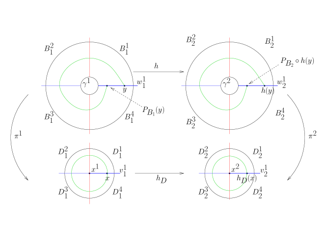
Figure 12: The closed curve starting at $x\in v_{1}^{1}$ lift by the maps $\eta_{s}$ to a curve that connects $y=\eta_{1}(x)$ with $P_{B_{1}}(y)=\eta_{4}(x)$.

Let $V\subset\pi^{1}(\mathring{U}_{1})\cup\{x^{1}\}$ be a neighbourhood of $x^{1}$. We will start by constricting $h_{D}$ in each quadrant $V\cap D_{1}^{s}$. For every $s=1,\dots,4$ let $h_{D}^{s}:V\cap D_{1}^{s}\to D_{2}^{s}$ be defined in the following way:

$$h_{D}^{s}(x)=\left\{\begin{array}[]{lcc}\pi^{2}_{s}\circ h\circ\eta_{s}(x)&\text{if}&x\neq x^{1},\\ \\ x^{2}&\text{if}&x=x^{1}.\\ \end{array}\right.$$ (21)

We claim that each $h_{D}^{s}$ is a homeomorphism onto its image. Observe that $\eta_{s}$ takes points in $D_{1}^{s}\backslash\{x^{1}\}$ into the quadrant $B_{1}^{s}$, $h$ takes points in $B_{1}^{s}$ into the quadrant $B_{2}^{s}$ and then $\pi^{2}$ projects $B_{2}^{s}$ into the punctured quadrant $D_{2}^{s}\backslash\{x^{2}\}$. Since each map is a homeomorphism onto its image then $h_{D}^{s}$ takes $V\cap D_{1}^{s}\backslash\{x^{1}\}$ homeomorphically onto its image in $D_{2}^{s}\backslash\{x^{2}\}$. Since the projections along the flow send points near $\gamma^{i}$ in the Birkhoff section to points near $x^{i}$ we see that $h_{D}^{s}$ is continuous in $x^{1}$ and the claim follows.

We define now $h_{D}:V\to D_{2}\text{ such that }$

$$h_{D}(x)=h_{D}^{s}(x)\text{ if }x\in D_{1}^{s},\ s=1,\dots,4.$$ (22)

We will show that $h$ is a well defined map, that is a homeomorphism onto its image and conjugates the first return maps $P_{D_{i}}$ for points close to $x^{i}$. To see that $h_{D}$ is well defined we have to check the definition of $h_{D}$ over the boundaries $v_{1}^{s}$, $s=1,\dots,4$ of the quadrants $D_{1}^{s}$. If $x$ belongs to some segment $v_{1}^{s}$ for $s=2,3,4$ then we have that $\eta_{s-1}(x)=\eta_{s}(x)$. This is because the maps $\pi^{i}_{s-1}$ and $\pi^{i}_{s}$ coincides over the segment $w_{i}^{s}$ which separates the quadrants $B_{i}^{s-1}$ and $B_{i}^{s}$. It follows that

$$h_{D}^{s}(x)=\pi^{2}_{s}\circ h\circ\eta_{s}(x)=\pi^{2}_{s-1}\circ h\circ\eta_{s-1}(x)=h_{D}^{s-1}(x),\text{ for every }x\in v_{1}^{s},$$

so the map $h_{D}$ is well defined in the segments $v_{1}^{2}$, $v_{1}^{3}$ and $v_{1}^{4}$.

We will use now proposition 3.14 to show that $h_{D}$ is well defined and continuous over the segment $v_{1}^{1}$. By this proposition we have that $\pi^{i}_{4}(z)=P_{D_{i}}^{-1}\circ\pi^{i}_{1}(z)=\pi^{i}_{1}\circ P_{B_{i}}^{-1}(z)$, for every $z\in w_{i}^{1}$. So it follows that $\eta_{4}(x)=P_{B_{i}}\circ\eta_{1}(x)$ for every $x\in v_{1}^{1}$, as we have illustrated in figure 12. Using that $h$ conjugates the maps $P_{B_{i}}$ we have that

$$h_{D}^{4}(x) =\pi_{4}^{2}\circ h\circ\eta_{4}(x)=\pi_{4}^{2}\circ h\circ P_{B_{1}}\circ\eta_{1}(x)$$ (23)

$$=\pi_{4}^{2}\circ P_{B_{2}}\circ h\circ\eta_{1}(x)=\pi_{1}^{2}\circ h\circ\eta_{1}(x)=h_{D}^{1}(x).$$ (24)

Since $h_{D}^{4}(x)=h_{D}^{1}(x)$ for every $x\in v_{1}^{1}$, we conclude that $h_{D}:V\to D_{2}$ is well defined, and is a homeomorphism onto its image.

To finish the proof, consider a disk $D_{1}^{\prime}\subset V$ that contains $x^{1}$ and define $D_{2}^{\prime}=h(D_{1}^{\prime})$. We have to show that the homeomorphism $h:D_{1}^{\prime}\to D_{2}^{\prime}$ is a local conjugation between $P_{D_{1}}$ and $P_{D_{2}}$. Let $x\in D_{1}^{\prime}$ be a point which belongs to some quadrant $D_{1}^{s}$. Then

$$h_{D}\circ P_{D_{1}}(x) =\pi^{2}_{s}\circ h\circ\eta_{s}\circ P_{D_{1}}(x)=\pi^{2}_{s}\circ h\circ P_{B_{1}}\circ\eta_{s}(x)$$ (25)

$$=\pi^{2}_{s}\circ P_{B_{2}}\circ h\circ\eta_{s}(x)=P_{D_{2}}\circ\pi^{2}_{s}\circ h\circ\eta_{s}(x)=P_{D_{2}}\circ h_{D}(x).$$ (26)

General case

The general case follows the same proof that the previous case, the only difference is when checking the continuity along the segment $v^{1}_{s}$ and the conjugation. Using proposition 3.14 we can see how to modify equations (23) and (25) above and obtain the desired result.

3.3 Proof of Theorem B (theorem 3.9).

Take two flows $\phi_{t}^{i}:M_{i}\to M_{i}$, $i=1,2$, equipped with Birkhoff sections $\iota_{i}:(\Sigma_{i},\partial\Sigma_{i})\to(M_{i},\Gamma_{i})$, as in the statement of theorem 3.9. We will prove theorem 3.9 assuming that $\Gamma_{i}$ consists in exactly one periodic orbit $\gamma^{i}\subset M_{i}$, since the general case follows by repeating the same argument in a neighbourhood of each periodic orbit in $\Gamma_{i}$.

By hypothesis $\Sigma_{1}$ and $\Sigma_{2}$ are homeomorphic, so each surface has the same number $p>0$ of boundary components. We call them $\partial\Sigma_{i}=C_{1}^{i}\cup\cdots\cup C_{p}^{i}$. By blowing down each surface $\Sigma_{i}$ we obtain a closed surface $\widehat{\Sigma}_{i}$ with a set $\Delta_{i}=\{x_{1}^{1},\dots,x_{p}^{i}\}$ of marked points, where each $x^{i}_{j}$ is the point obtained by collapsing the boundary component $C^{i}_{j}$, and a pseudo-Anosov homeomorphism $\hat{P}_{i}$ on $\widehat{\Sigma}_{i}$ fixing the set $\Delta_{i}$. Since the first return map of a Birkhoff induces a cyclic permutation of all the boundary components arriving to the same $\gamma^{i}\in\Gamma_{i}$ (proposition 3.14) then the finite set $\Delta_{i}$ constitutes a single periodic orbit of period $p$.

Since the actions induced by $P_{i}$ on $\pi_{1}(\Sigma_{i})$, $i=1,2$ are conjugated by the action of a homeomorphism $\Psi:\Sigma_{1}\to\Sigma_{2}$ (thus sending conjugacy classes of curves in $\partial\Sigma_{1}$ onto conjugacy classes of curves in $\partial\Sigma_{2}$) they induce conjugated elements $[P_{i}]$ in the mapping class group $\textsl{MCG}(\Sigma_{i},\Delta_{i})$ of the punctured surface. We recall that this is the group of homeomorphisms of $\Sigma_{i}$ fixing $\Delta_{i}$, up to homotopies fixing $\Delta_{i}$, see section 2.4. Since the $\hat{P}_{i}$ are pseudo-Anosov then, by proposition 2.18 there exists a homeomorphism $h:\widehat{\Sigma}_{1}\to\widehat{\Sigma}_{2}$ such that $h(\Delta_{1})=\Delta_{2}$ and $\hat{P}_{2}\circ h=h\circ\hat{P_{1}}$. In particular, we deduce equality on linking numbers: $n(\gamma^{1},\Sigma_{1})=n(\gamma^{2},\Sigma_{2})=n$.

To obtain the desired orbital equivalence $(\phi_{t}^{1},M_{1})\to(\phi_{t}^{2},M_{2})$,

Case I: Assume that each $\Sigma_{i}$ is tame.

The homeomorphism $h:\mathring{\Sigma}_{1}\to\mathring{\Sigma}_{2}$ that conjugates the first return maps $P_{i}$ produces an orbital equivalence $H:(\phi_{t}^{1},M_{1}\backslash\gamma^{1})\to(\phi_{t}^{2},M_{2}\backslash\gamma^{2})$, which satisfies that $H(x)=h(x)$, for every $x\in\mathring{\Sigma_{1}}$.

Claim.

Under the assumption that the sections are tame and $m(\gamma^{1},\Sigma_{1})=m(\gamma^{2},\Sigma_{2})$, for every neighbourhood $W$ of $\gamma^{1}$ there exists a homeomorphism $H_{W}:M_{1}\to M_{2}$ such that:

1. $H_{W}$ is a topological equivalence between $(\phi_{t}^{1},M_{1})$ and $(\phi_{t}^{2},M_{2})$;

2. $H_{W}(x)=h(x)$, for every $x\in\Sigma_{1}\backslash W$.

Proof.

Let $W_{1}=W$, $W_{2}:=H(W_{1}\backslash\gamma^{1})\cup\gamma^{2}$ and consider the restriction $H:W_{1}\backslash\gamma^{1}\to W_{2}\backslash\gamma^{2}$. Then, this homeomorphism is an orbital equivalence between the (open) sets $W_{i}\backslash\gamma^{i}$. More over, if we call $B_{1}^{1}$ to one of the components of $\iota_{1}(\Sigma_{1})\cap W_{1}$ and $B_{1}^{2}=\tilde{h}(B_{1}^{1})$, then $H$ coincides with $h$ over $B_{1}\backslash\gamma^{1}$ and $h$ is a local conjugation between the first return maps to the local sections $B_{1}^{i}$. So we are in the hypothesis of theorem 3.20. Given an arbitrary neighbourhood $N\subset W_{1}$, there exists then a local orbital equivalence $H_{N}:W_{1}\to W_{2}$ such that $H_{N}(x)=H(x)$, for every $x\in W_{1}\backslash N$. We define $H_{W}:M_{1}\to M_{2}$ such that

$$H_{W}(x)=\left\{\begin{array}[]{lcc}&H_{N}(x),&\text{ if }x\in W_{1}\\ &H(x),&\text{ if }x\in M_{1}\backslash N.\end{array}\right.$$

Then $H_{W}$ is a well defined homeomorphism, and is an orbital equivalence. Observe that, since $H_{W}$ coincides with $H$ outside $N$, then $H_{W}(x)=h(x)$, for every $x\in\Sigma_{1}\backslash W$. This finishes the proof in the case of tame sections. ∎

Case II: General case.

If the sections $\Sigma_{i}$, $i=1,2$ given in the statement of theorem 3.9 are not tame, we can modify them in a neighbourhood of the boundary and produce tame Birkhoff sections $\Sigma_{i}^{\prime}$, without altering the action of the first return map on the fundamental group.

More concretely, for each $\gamma_{i}$ consider two tubular neighbourhoods $N_{i}\subset W_{i}$ satisfying that for every $x\in\Sigma_{i}\backslash W_{i}$ then the $\phi_{t}^{i}$-orbit segment $[x,P_{i}(x)]$ connecting $x$ with its first return to $\Sigma_{i}$, is completely contained in $M_{i}\backslash N_{i}$. By proposition 3.19 there exists a Birkhoff section $\Sigma_{i}^{\prime}$ for $(\phi_{t}^{i},M_{i})$ that is tame and coincides with $\Sigma_{i}$ in the complement of $N_{i}$. Denote $\Sigma_{0}=\Sigma_{i}^{\prime}\backslash W_{i}\equiv\Sigma_{i}\backslash W_{i}$. Denote by $P_{i}^{\prime}:\Sigma_{i}^{\prime}\to\Sigma_{i}^{\prime}$ the first return map. Then, it follows that $P_{i}^{\prime}(x)=P_{i}(x)$, for every $x\in\Sigma_{0}$. Moreover, since $\Sigma_{0}$ is a deformation retract of both surfaces $\Sigma_{i}$ and $\Sigma_{i}^{\prime}$, every homotopy class of closed curve in any of the surfaces has a representative $\alpha$ completely contained in $\Sigma_{0}$ and it follows that $P_{i}^{\prime}(\alpha)=P_{i}(\alpha)$. Thus, $P_{i}$ and $P_{i}^{\prime}$ induce equivalent actions on $\pi_{1}(\Sigma_{i})$ and $\pi_{1}(\Sigma_{i}^{\prime})$, respectively.

We obtain tame Birkhoff sections satisfying the hypothesis of theorem 3.9, and we conclude as in the previous case.

4 Almost-Anosov structures.

Let $(\phi_{t},M)$ be a transitive topological Anosov flow. In the complement of some finite collections of periodic orbits, it is possible to define a smooth atlas and a Riemannian metric such that the restriction of the flow onto this set is orbitally equivalent to a smooth flow preserving a uniformly hyperbolic splitting. This follows from the existence of Birkhoff sections, theorem 3.2. Since $\phi_{t}$ is transitive, there exists a Birkhoff section $\iota:(\Sigma,\partial\Sigma)\rightarrow(M,\Gamma).$ In the complement of $\Gamma$ the restriction of the flow is orbitally equivalent to the suspension of the first return map $P:\mathring{\Sigma}\to\mathring{\Sigma}$. Since this map is obtained by blowing-up a pseudo-Anosov homeomorphism $\widehat{P}:\widehat{\Sigma}\to\widehat{\Sigma}$ on a closed surface, it is possible to define a convenient smooth structure and Riemannian metric on the (open) manifold $M\backslash\Gamma$, as we explain below in 4.1. We will be interested in a description of this smooth atlas in a neighbourhood of each singular orbit $\gamma\in\Gamma$, where the atlas is not defined. This will be the content of subsection 4.2.

4.1 Almost-Anosov atlas induced by a Birkhoff section.

From now on we will denote $M_{\Gamma}=M\backslash\Gamma$ and, in general, we will use $\Gamma$ as a sub-index for referring to the objects associated to the restriction of $\phi_{t}$ onto $M_{\Gamma}$.

Proposition 4.1.

In $M_{\Gamma}$ there exists a smooth atlas $\mathcal{D}_{\Gamma}$ such that:

1. The foliation by flow orbits $\mathcal{O}_{\Gamma}$ on $M_{\Gamma}$ is tangent to a smooth non-singular vector field $X_{\Gamma}$.

2. $D\phi_{t}^{X_{\Gamma}}:TM_{\Gamma}\to TM_{\Gamma}$ preserves a splitting $TM_{\Gamma}=E^{s}_{\Gamma}\oplus E^{c}_{\Gamma}\oplus E^{u}_{\Gamma}$, where $\phi_{t}^{X_{\Gamma}}$ denotes the flow generated by $X_{\Gamma}$ and the bundle $E^{c}_{\Gamma}$ is collinear with this vectorfield.

3. There exists a Riemannian metric $|\cdot|_{\Gamma}$ in the (open) manifold $M_{\Gamma}$ for which the splitting is uniformly hyperbolic and

   $$|D\phi_{t}^{X_{\Gamma}}(p)\cdot v|_{\Gamma}=\lambda^{t}\cdot|v|_{\Gamma},\ \forall\ v\in E^{s}\text{ and }t\geq 0,$$

   $$|D\phi_{t}^{X_{\Gamma}}(p)\cdot v|_{\Gamma}=\lambda^{-t}\cdot|v|_{\Gamma},\ \forall\ v\in E^{u}\text{ and }t\leq 0,$$

   where $0<\lambda<1$ is the stretching factor of $P$.

Definition 4.2.

The smooth atlas $\mathcal{D}_{\Gamma}$ stated in proposition 4.1 above is called an almost Anosov structure for $(\phi_{t},M)$, induced by the Birkhoff section $\iota:(\Sigma,\partial\Sigma)\rightarrow(M,\Gamma).$

Proof.

To prove the proposition, observe that since the blow down $\widehat{P}:\widehat{\Sigma}\to\widehat{\Sigma}$ is pseudo-Anosov it has an associated pair $(\mathcal{F}^{s},\mu_{s})$ and $(\mathcal{F}^{u},\mu_{u})$ of transverse foliations equipped with transverse measures and a stretching factor $0<\lambda<1$. Since there are no singularities on the open surface $\mathring{\Sigma}=\widehat{\Sigma}\backslash\Delta$, where $\Delta$ is the finite set obtained by blowing-down the components of $\partial\Sigma$, this pair of transverse foliations provides a translation atlas

$$\mathcal{D}_{\Delta}=\{\varphi_{i}:U_{i}\to\mathbb{R}^{2}\}_{i\in I},\text{ where }\{U_{i}\}_{i\in I}\text{ is an open cover of }\mathring{\Sigma},$$

such that, on each coordinate neighbourhood, the foliations $\mathcal{F}^{s}$ and $\mathcal{F}^{u}$ correspond to the foliations of the plane by horizontal and vertical lines, and the transverse measures $\mu_{s}$ and $\mu_{u}$ correspond to integrate the 1-forms $|dx|$ and $|dy|$ in $\mathbb{R}^{2}$, respectively. This translation atlas defines a smooth structure in $\mathring{\Sigma}$ and a Riemannian metric $|\cdot|^{2}={dx^{2}+dy^{2}}$. In the local coordinates of this atlas, the first return $P:\mathring{\Sigma}\to\mathring{\Sigma}$ takes the form of a homeomorphism

$$\varphi_{i}\circ P\circ\varphi_{j}^{-1}:(x,y)\mapsto\pm\begin{pmatrix}\lambda&0\\ 0&\lambda^{-1}\end{pmatrix}(x,y)+\tau_{ij}$$

between open sets in $\mathbb{R}^{2}$. It follows that $P$ is smooth and $DP:T\mathring{\Sigma}\to T\mathring{\Sigma}$ preserves a splitting $T\mathring{\Sigma}=E^{s}\oplus E^{u}$ given in local coordinates by $E^{s}=\mathbb{R}\times 0$ and $E^{u}=0\times\mathbb{R}$. Moreover, with the metric $|\cdot|$ this splitting is uniformly hyperbolic.

Consider the suspension flow $(\mathring{\phi}_{t},\mathring{M})=\textrm{suspension}\left(P:\mathring{\Sigma}\to\mathring{\Sigma}\right)$. With the structure of smooth Riemannian manifold on $\mathring{\Sigma}$ defined above, $\phi_{t}$ is the flow generated by the smooth vector field $\partial/\partial t$ on the smooth (open) manifold $\mathring{M}=\mathring{\Sigma}\times\mathbb{R}/{(z,t)\sim(P(z),t-1)}.$ The $DP$-invariant splitting on the surface induces a splitting of the form $T\mathring{M}=E^{s}\oplus E^{u}\oplus\textsl{span}\{\partial/\partial t\}$ that is invariant by $D\mathring{\phi}_{t}$. In addition, for each point $(z,t)$ of $\mathring{\Sigma}\times\mathbb{R}$, the expression $|\cdot|^{2}=\lambda^{-2t}dx^{2}+\lambda^{2t}dy^{2}+dt^{2}$ defines a Riemannian metric that pushes-down to the quotient manifold $\mathring{M}$ and induces a metric $|\cdot|_{\circ}$ that coincides with the metric on $\mathring{\Sigma}$ along a fixed global transverse section $\mathring{\Sigma}\hookrightarrow\mathring{M}$. The invariant splitting of $T\mathring{M}$ is uniformly hyperbolic with respect to this metric, and it follows from its definition that $|D\phi_{t}|_{E^{s}}|_{\circ}=\lambda^{t}$ and $|D\phi_{t}|_{E^{u}}|_{\circ}=\lambda^{-t}$. Since $(\phi_{t},M_{\Gamma})$ is orbitally equivalent to $(\mathring{\phi}_{t},\mathring{M})$, this completes the proof. ∎

Remark 4.3.

Not every finite set $\Gamma$ of periodic orbits bounds a Birkhoff section. For example, this is the case of a single periodic orbit in a suspension Anosov flow, since it represents a non-trivial homology class on the phase space. This says that the almost Anosov structures associated to a given topological Anosov flow are not arbitrary objects, but they have some intricate relation with the topology of the flow.

4.2 Normal form in a neighbourhood of $\gamma\in\Gamma$.

We describe here a normal form for the vector field $X_{\Gamma}$ given in proposition 4.1, in a neighbourhood of each $\gamma\in\Gamma$. Fix some periodic orbit $\gamma\in\Gamma$ and consider some small tubular neighbourhood $W$. We will assume that the invariant local manifolds are orientable, so every small tubular neighbourhood $W$ is partitioned in four quadrants $W_{i}$, $i=1,\dots,4$. The following proposition gives a normal form for the vector field $X_{\Gamma}$ on the punctured neighbourhood $W\setminus\gamma$. The normal form will be constructed by glueing along the boundaries (in a non trivial way) the four quadrants of a saddle type periodic orbit, generated by an affine vectorfield in $\mathbb{R}^{2}\times\mathbb{R}/\mathbb{Z}$.

Recall that the first return to $\Sigma$ is pseudo-Anosov and we denote by $0<\lambda<1$ its stretching factor. Also recall that $\gamma$ is the image of a number $p=p(\gamma,\Sigma)$ of connected components of $\partial\Sigma$. This means that in a small neighbourhood $W$ of $\gamma$ the surface $\Sigma\cap W$ splits as $p$ different local Birkhoff sections at $\gamma$, each of them with the same linking number $n=n(\gamma,\Sigma)$ and multiplicity $m=m(\gamma,\Sigma)$.

Proposition 4.4.

Let $(\phi_{t},M)$ be transitive topological Anosov flow and $\iota:(\Sigma,\partial\Sigma)\to(M,\Gamma)$ a Birkhoff section. Consider the smooth atlas $\mathcal{D}_{\Gamma}$ and the smooth vector field $X_{\Gamma}$ on $M\backslash\Gamma$ induced by the Birkhoff section (cf. proposition 4.1). Then, for every $\gamma\in\Gamma$ there exists a small tubular neighbourhood $W$, divided in four quadrants $W_{i}$, $i=1,\dots,4$, and a systems of smooth charts

$$\Pi_{i}:W_{i}\setminus\gamma\to\left(\mathbb{D}_{i}\setminus\{0\}\right)\times\mathbb{R}/\mathbb{Z},\ i=1,\dots,4$$ (27)

satisfying that:

1. $D\Pi_{*}(X_{\Gamma})=X_{(\lambda,p,n)}$, where $X_{(\lambda,p,n)}:\mathbb{R}^{2}\times\mathbb{R}/\mathbb{Z}\to\mathbb{R}^{3}$ is the vector field

   $$X_{(\lambda,p,n)}(x,y,z)=\left(\log(\lambda)x,-\log(\lambda)y,\frac{1}{np}\right).$$ (28)

2. The charts $\Pi_{i}$ send each connected component of $\Sigma\cap(W\backslash\gamma)$ isometrically onto a surface of the form $\left(U\times 0\right)\cap\left(\mathbb{D}_{i}\backslash\{0\}\right)\times\left\{\frac{k}{np}\right\}$, where $U$ is an open neighbourhood of $0\in\mathbb{R}^{2}$, $k\in\{0,\dots,np-1\}$.

3. It is verified that:

   $$\Pi_{1}(W_{1})\cap\Pi_{2}(W_{2})=\{0\}\times(0,+\infty)\times\mathbb{R}/\mathbb{Z}$$

   $$\Pi_{2}(W_{2})\cap\Pi_{3}(W_{3})=(-\infty,0)\times\{0\}\times\mathbb{R}/\mathbb{Z}$$

   $$\Pi_{3}(W_{3})\cap\Pi_{4}(W_{4})=\{0\}\times(-\infty,0)\times\mathbb{R}/\mathbb{Z}$$

   $$\Pi_{4}(W_{4})\cap\Pi_{1}(W_{1})=(0,+\infty)\times\{0\}\times\mathbb{R}/\mathbb{Z}$$

   and

   $$\Pi_{2}\circ\Pi_{1}^{-1}:(0,y,z)\mapsto(0,y,z)$$

   $$\Pi_{3}\circ\Pi_{2}^{-1}:(x,0,z)\mapsto(x,0,z)$$ (29)

   $$\Pi_{4}\circ\Pi_{3}^{-1}:(0,y,z)\mapsto(0,y,z)$$

   $$\Pi_{1}\circ\Pi_{4}^{-1}:(x,0,z)\mapsto\left(x,0,z+\frac{m}{n}\right).$$

Remark 4.5.

The charts defined in proposition 4.4 send the orbit segments of $\phi_{t}$ that lie inside each punctured quadrant $W_{i}\setminus\gamma$ onto the orbit segments of the flow generated by the vector field (28) inside the quadrant $\mathbb{D}_{i}\times\mathbb{R}/\mathbb{Z}$ preserving the time parameter. Thus, we can reconstruct the vector field $X_{\Gamma}$ in $W\backslash\gamma$ by glueing the four pieces

$$\left(X_{(\lambda,p,n)}\ ,(\mathbb{D}_{i}\backslash\{0\})\times\mathbb{R}/\mathbb{Z}\right),\ i=1,\dots,4$$

along their boundaries in the way specified in (3). Since the vector field $X_{(\lambda,p,n)}$ is invariant by vertical translations, the glueing map $\Pi_{1}\circ\Pi_{4}^{-1}$ preserves $X_{(\lambda,p,n)}$ and we get a well defined vector field in the quotient manifold, which is homeomorphic to a solid torus with an essential closed curve on the interior removed.

Proof of proposition 4.1.

We assume first that $p(\gamma,\Sigma)=1$. Choose a small tubular neighbourhood $W$ of $\gamma$ such that $B=\Sigma\cap W$ is a connected local Birkhoff section, equipped with a first return map $P_{B}:U\backslash\gamma\to B\backslash\gamma$ (cf. definition 3.10 for notations). Denote by $\widehat{B}$ the disk obtained by blowing-down $B$ along $\gamma$ and let $\widehat{P}_{B}:\widehat{U}\to\widehat{B}$ be the corresponding map. Since $\widehat{P}_{B}$ is a local homeomorphism with a fixed point $q\in\widehat{U}$ of multi-saddle type (with $2n(\Sigma,\gamma)$ prongs), by suspending we obtain a germ $(\widehat{\phi}_{t},\widehat{W})_{\widehat{\gamma}}$ of a flow $\widehat{\phi}_{t}$ around a multi-saddle periodic orbit $\widehat{\gamma}\subset\widehat{W}$, where $\widehat{W}\simeq\mathbb{D}^{2}\times\mathbb{R}/\mathbb{Z}$ (cf. section 2). Up to shrinking the neighbourhoods $W$ and $\widehat{W}$ if necessary, there is a local orbital equivalence

$$\left(\phi_{t},W\backslash\gamma\right)\to\left(\widehat{\phi}_{t},\widehat{W}\backslash\widehat{\gamma}\right)$$

between the respective complements of $\gamma$ and $\widehat{\gamma}$, that takes the surface $B\backslash\gamma$ onto $\widehat{B}\backslash\{q\}$. In particular, observe that the local invariant manifolds of $\widehat{\gamma}$ partition $\widehat{W}\backslash\widehat{\gamma}$ in four quadrants $\widehat{W}_{i}$, $i=1,\dots,4$. The smooth atlas and the metric in $W\backslash\gamma$ given in proposition 4.1 are defined by pulling back those on $\widehat{W}\backslash\widehat{\gamma}$. Thus, it suffices to check 4.4 using $\left(\widehat{\phi}_{t},\widehat{W}\backslash\widehat{\gamma}\right)$.

Following the description in section 3, the disk $\widehat{B}$ is divided in $4n$ quadrants, that we enumerate as $\widehat{B}_{1},\dots,\widehat{B}_{4n}$ following the positive circular order. On each $\widehat{W}_{i}$, $i=1,\dots,4$ there are contained exactly $n$ quadrants of the form $\widehat{B}_{i+4j}$, $j=0,\dots,n-1$. All of these quadrants share the common vertex $q$. Consider the sets $\widehat{B}_{i+4j}^{*}=\widehat{B}_{i+4j}\setminus\{q\},$ that we call punctured quadrants. These are a collection of pairwise disjoint surfaces, properly embedded in the manifold $\widehat{W}_{i}\backslash\widehat{\gamma}$, each one homeomorphic to a disk. By proposition 3.14 then $\widehat{P}$ permutes cyclically these surfaces and $\widehat{P}^{n}$ preserves each of them. So each $\widehat{B}_{i+4j}^{*}$ is a transverse section for $\widehat{\phi}_{t}$ on $\widehat{W}_{i}\setminus\widehat{\gamma}$, with first return defined for points near $\hat{x}$ and return time constant and equal to $n$. It follows that there is a smooth time-preserving conjugation between $\left(\widehat{\phi}_{t}\ ,\widehat{W}_{i}\setminus\widehat{\gamma}\right)$ and the flow induced by $z\mapsto z+t$ in

$$\widehat{B}_{i+4j}^{*}\times\mathbb{R}/_{(z,t)\mapsto(\widehat{P}^{n}(z),t-|n|)}.$$ (30)

In addition, since $\widehat{P}_{B}$ is the restriction of a pseudo-Anosov homeomorphism $\widehat{P}:\widehat{\Sigma}\to\widehat{\Sigma}$ with stretching factor $\lambda$ and $q$ is a $2n$-prong, there exists a chart $\varphi_{q}:(\widehat{B},q)\to(\mathbb{R}^{2},0)$ that is smooth outside $\{q\}$ and satisfies:

1. $\varphi_{q}:\widehat{B}\setminus\{q\}\to\mathbb{R}^{2}\setminus\{0\}$ is a $n$-fold covering,

2. $A\circ\varphi_{q}(p)=\varphi_{q}\circ\widehat{P}(p)$, for every $p$ in a neighbourhood of $q$, where $A=\begin{pmatrix}\lambda&0\\ 0&\lambda^{-1}\end{pmatrix}$.

3. For every $i=1,\dots,4$, the chart $\varphi_{q}$ sends $\widehat{B}_{i+4j}$ isometrically onto its image in $\mathbb{D}_{i}\subset\mathbb{R}^{2}$.

In particular, the chart $\varphi_{q}$ provides a smooth conjugation quadrant by quadrant:

$$\leavevmode\hbox to75.76pt{\vbox to51.58pt{\text{[drawing]}}}\ \text{for every}\ i=1,\dots,4. {\widehat{B}_{i+4j}} {\widehat{B}_{i+4j}} {\mathbb{D}_{i}} {\mathbb{D}_{i}} \scriptstyle{\widehat{P}^{n}} \scriptstyle{\varphi_{q}} \scriptstyle{\varphi_{q}} \scriptstyle{A^{n}} {\widehat{B}_{i+4j}} {\widehat{B}_{i+4j}} {\mathbb{D}_{i}} {\mathbb{D}_{i}} \scriptstyle{\widehat{P}^{n}} \scriptstyle{\varphi_{q}} \scriptstyle{\varphi_{q}} \scriptstyle{A^{n}}$$

and therefore the flow in (30) above is conjugated to the flow generated by $z\mapsto z+t$ in

$$\mathbb{D}_{i}\times\mathbb{R}/_{(z,t)\mapsto(A^{n}(z),t-|n|)}.$$ (31)

Since this latter flow is smoothly time-preserving equivalent to the germ of the vector field $X_{(\lambda,n)}(x,y,z)=(\log(\lambda)x,-\log(\lambda)y,1/n)$ on the quadrant $\mathbb{D}_{i}\times\mathbb{R}/\mathbb{Z}$, we obtain a family of charts

$$\Pi_{i}^{j}:\widehat{W}_{i}\backslash\widehat{\gamma}\to(\mathbb{D}_{i}\backslash\{0\})\times\mathbb{R}/\mathbb{Z},\ j=0,\dots,n-1,$$

satisfying the desired properties. Each chart is induced from one of the maps $\widehat{P}^{n}:\widehat{B}^{*}_{i+4j}\to\widehat{B}^{*}_{i+4j}$.

We may assume that the coordinate charts $\Pi_{i}$ send each surface $\widehat{B}^{*}_{i+4j}$ inside a plane of the form $\mathbb{D}_{i}\times\{j/n\}$, for every $j=0,\dots,n-1$. Chose $\widehat{B}^{*}_{1}$ in the quadrant $\widehat{W}_{1}$ and $\Pi_{1}$ such that $\Pi_{1}:\widehat{B}^{*}_{1}\mapsto\mathbb{D}_{1}\times\{0\}$. Observe that the chart $\varphi_{q}$ extends over the union

$$\widehat{B}^{*}_{1}\cup\widehat{B}^{*}_{2}\cup\widehat{B}^{*}_{3}\cup\widehat{B}^{*}_{4}$$

sending each $\widehat{B}^{*}_{i}$ onto $\mathbb{D}_{i}\times\{0\}$. Thus, we can coherently extend $\Pi_{1}$ to the adjacent quadrants $\widehat{W}_{i}\setminus\widehat{\gamma}$, $i=2,3,4$, in such a way that each $\Pi_{i}$ sends the surface $\widehat{B}^{*}_{i}$ to $\mathbb{D}_{i}\times\{0\}$. The quadrant $\widehat{B}^{*}_{4}$ contained in $\widehat{W}_{4}$ is adjacent to some quadrant $\widehat{B}^{*}_{5}$ in $\widehat{W}_{1}$. By proposition 3.14 we see that $\widehat{B}^{*}_{5}$ coincides with $\mathbb{D}_{1}\times\{m/n\}$, provided $\Pi_{1}(\widehat{B}^{*}_{1})=\mathbb{D}_{1}\times\{0\}$. Thus, the holonomy defect of $\Pi_{4}\circ\Pi_{1}^{-1}$ on the common boundary $\widehat{W}_{4}\cap\widehat{W}_{1}$ is a vertical translation by $\frac{m}{n}$.

This completes the proof of the lemma assuming that $p(\gamma,\Sigma)=1$. If there are more than one boundary components of $\Sigma$ that cover $\gamma$, the argument is the same but the first return map to each $\widehat{B}^{*}_{i+4j}$ changes by $\widehat{P}^{p(\gamma,\Sigma)\cdot n}$, so we must modify the parameters of $X_{(n,\lambda)}$ in the appropriated way. ∎

5 Construction of the hyperbolic models

Consider a transitive topological Anosov flow $(\phi_{t},M)$. In this section we construct another flow $(\psi_{t},N)$ which is smooth, Anosov, volume preserving and orbitally equivalent to the first one. We start by sketching the general argument, and we develop the steps in the following subsections.

5.1 Proof of theorem A.

Choose a tame Birkhoff section $\iota:(\Sigma,\partial\Sigma)\to(M,\Gamma)$ with first return $P:\mathring{\Sigma}\to\mathring{\Sigma}$ for the flow $(\phi_{t},M)$, as given in theorem 3.2 and proposition 3.19. Then, the constructions in propositions 4.1 and 4.4 associates:

1. A smooth atlas $\mathcal{D}_{\Gamma}$ and a Riemannian metric $|\cdot|_{\Gamma}$ on the manifold $M\setminus\Gamma$ such that, up to reprametrization, the restriction of $\phi_{t}$ onto $M\backslash\Gamma$ is generated by a smooth vector field $X_{\Gamma}$ and preserves a uniformly hyperbolic splitting $E^{s}_{\Gamma}\oplus E^{c}_{\Gamma}\oplus E^{u}_{\Gamma}$. Moreover,

   $$|D{\phi}_{t}(v)|_{\Gamma}=\lambda^{t}|v|_{\Gamma},\ \forall\ v\in E^{s}_{\Gamma},\ t\geq 0,$$

   $$|D{\phi}_{t}(v)|_{\Gamma}=\lambda^{-t}|v|_{\Gamma},\ \forall\ v\in E^{u}_{\Gamma}\ t\leq 0,$$

   where $0<\lambda<1$ is the stretching factor of the first return map to the Birkhoff section.

2. For every orbit $\gamma\in\Gamma$ there is a small tubular neighbourhood $W$, divided in four quadrants $W_{i}$, $i=1,\dots,4$, and a system of smooth charts

   $$\Pi_{i}:W_{i}\setminus\gamma\to(\mathbb{D}_{i}\setminus\{0\})\times\mathbb{R}/\mathbb{Z},\ i=1,\dots,4$$ (32)

   called normal coordinates, verifying that:

   1. $D\Pi_{i}:X_{\Gamma}\mapsto X_{(\lambda,n,p)}$, $D\Pi_{i}:E^{s}_{\Gamma}\mapsto\mathbb{R}\times 0\times 0$ and $D\Pi_{i}:E^{u}_{\Gamma}\mapsto 0\times\mathbb{R}\times 0$, where

      $$X_{(\lambda,n,p)}(x,y,z)=\left(\ \log(\lambda)x\ ,\ -\log(\lambda)y\ ,\ \frac{1}{np}\ \right)\ \ \text{on}\ \ \ \mathbb{R}^{2}\times\mathbb{R}/\mathbb{Z};$$ (33)

   2. The charts $\Pi_{i}$ send the quadrants of the local Birkhoff section $\Sigma\cap W\backslash\gamma$ isometrically onto surfaces of the form $\left(\mathbb{D}_{i}\setminus\{0\}\right)\times\left\{\frac{k}{np}\right\}$ with $k=0,\dots,np-1$;

   3. Along the corresponding domains of intersection between the four quadrants, we have

      $$\Pi_{2}\circ\Pi_{1}^{-1}:(x,y,z)\mapsto(x,y,z)$$

      $$\Pi_{3}\circ\Pi_{2}^{-1}:(x,y,z)\mapsto(x,y,z)$$

      $$\Pi_{4}\circ\Pi_{3}^{-1}:(x,y,z)\mapsto(x,y,z)$$

      $$\Pi_{1}\circ\Pi_{4}^{-1}:(x,y,z)\mapsto\left(x,y,z+\frac{m}{n}\right);$$

   where $p=p(\gamma,\Sigma)$, $n=n(\gamma,\Sigma)$ and $m=m(\gamma,\Sigma)$ are the combinatorial parameters of the Birkhoff section at $\gamma$ (see section 3 for definitions).

Assumption: For simplicity, from now on and for the rest of the section we assume that $\Gamma$ consists in only one periodic orbit $\gamma$. We will assume as well that the local invariant manifolds of $\gamma$ are orientable (cf. remark 3.3). The general case can be derived from the present case, by applying the following construction on a neighbourhood of each curve $\gamma\in\Gamma$.

From the one side, using the charts given above in (32) we will define a family $R(r_{1},r_{2})\subset M$ of tubular neighbourhoods of $\gamma$, depending on two parameters $0<r_{2}<r_{1}$. From the other side, we will consider the affine vector field $X_{(\lambda,n,p)}$ given in equation (33) above, defined for all points in $\mathbb{R}^{2}\times\mathbb{R}/\mathbb{Z}$, and we will define a family $\mathbb{V}(r_{1},r_{2})\subset\mathbb{R}^{2}\times\mathbb{R}/\mathbb{Z}$ of tubular neighbourhoods of the saddle type periodic orbit $\gamma_{0}=\{0\}\times\mathbb{R}/\mathbb{Z}$, depending on two parameters $0<r_{2}<r_{1}$. This will be the content of subsection 5.2.

Now, for some fixed parameters $0<r_{2}<r_{1}<1$, consider the smooth manifold $M_{R}(r_{1},r_{2})$ obtained from $M$ by removing the interior of $R(r_{1},r_{2})$, equipped with the restriction of the vector field $X_{\Gamma}$. The construction is the following:

• Using the system of normal coordinates $\{\Pi_{i}:i=1,\dots,4\}$ we will define a diffeomorphism

  $$\varphi:\partial M_{R}(r_{1},r_{2})\to\partial\mathbb{V}(r_{1},r_{2})$$

  from the boundary of $M_{R}(r_{1},r_{2})$ to the boundary of $\mathbb{V}(r_{1},r_{2})$, that will depend on the signature of the multiplicity $m(\gamma,\Sigma)$. Glueing along the boundaries with $\varphi$ will produce a closed manifold

  $$N=N(r_{1},r_{2})\coloneqq M_{R}(r_{1},r_{2})\sqcup_{\varphi}\mathbb{V}(r_{1},r_{2})$$

  endowed with a smooth atlas. The vector fields $X_{\Gamma}$ on $M_{R}(r_{1},r_{2})$ and $X_{(\lambda,n,p)}$ on $\mathbb{V}(r_{1},r_{2})$ match together along the boundary and induce a smooth vector field $Y$ on $N$. In addition, the flow associated to $Y$ preserves a smooth volume form. This is the content of section 5.3.

• Let $(\psi_{t},N)$ be the flow generated by the vector field $Y$. In section 5.4 we will show that, for sufficiently small values of the parameters $0<r_{2}<r_{1}<1$, this flow is Anosov. This is basically a consequence of the hyperbolicity of $X_{\Gamma}$ away from $\gamma$ and the hyperbolicity of $X_{(\lambda,n,p)}$ near $\gamma_{0}$, and the argument will be carried out using the so called cone-field criterion. Remark that, since $\psi_{t}$ is smooth Anosov and preserves a smooth volume form, then it is ergodic (cf. [18]).

• Finally, in section 5.5, we will show that $(\psi_{t},N)$ is orbitally equivalent to the original topological Anosov flow $(\phi_{t},M)$. For proving this we will show that both flows can be equipped with adequate Birkhoff sections, where we can check the criterion in theorem B.

Theorem A follows then from the statements (1),(2) and (3) above.

5.2 Cross-shaped neighbourhoods.

We describe here a class of compact tubular neighbourhoods of a saddle type periodic orbit, that we call cross-shaped neighbourhood and will be used in the course of the proof of theorem A. We do it for both a regular periodic orbit of an affine vector field in euclidean space, and for the singular orbit $\gamma\in\Gamma$ using the charts in (32) above.

5.2.1 Affine model on $\mathbb{R}^{2}\times\mathbb{R}/\mathbb{Z}$.

Given $0<\lambda<1$ and two integers $n,p\geq 1$, consider the vector field $X=X_{(\lambda,n,p)}$ on $\mathbb{R}^{2}\times\mathbb{R}/\mathbb{Z}$ defined by $X_{(\lambda,n,p)}(x,y,z)=\left(\log(\lambda)x,-\log(\lambda)y,\frac{1}{np}\right).$ The corresponding flow is given by $\phi_{t}^{X_{(\lambda,n,p)}}(x,y,z)=(\lambda^{t}x,\lambda^{-t}y,z+t/np)$, so it splits as a linear flow on $\mathbb{R}^{2}$ times a translation flow on $\mathbb{R}/\mathbb{Z}$.

Remark 5.1.

It follows that:

1. The plane $\mathbb{R}^{2}\times\{0\}$ is a global transverse section, the first return map is the linear transformation $(x,y)\mapsto(\lambda^{np}x,\lambda^{-np}y)$, and the returning time is constant and equal to $np$.

2. The non-wandering set consists in one saddle type, hyperbolic, periodic orbit $\gamma_{0}$, that coincides point-wise with the set $\{0\}\times\mathbb{R}/\mathbb{Z}$. The stable and unstable manifolds are the cylinders

   $$W^{s}(\gamma_{0})=\mathbb{R}\times\{0\}\times\mathbb{R}/\mathbb{Z}$$

   $$W^{u}(\gamma_{0})=\{0\}\times\mathbb{R}\times\mathbb{R}/\mathbb{Z}$$

3. The action of $D\phi_{t}^{X_{(\lambda,n,p)}}$ on $\mathbb{R}^{3}$ preserves a splitting $E^{s}\oplus E^{c}\oplus E^{u}$ into three line bundles

   $$E^{s}=\mathbb{R}\times\{0\}\times\{0\},\ E^{u}=\{0\}\times\mathbb{R}\times\{0\}\ \text{and}\ E^{c}=\textsl{span}\{{X_{(\lambda,n,p)}}\},$$

   and for every $p\in\mathbb{R}^{2}\times\mathbb{R}/\mathbb{Z}$ we have that

   $$\|D\phi_{t}^{X_{(\lambda,n,p)}}(p)\cdot v\|=\lambda^{t}\cdot\|v\|,\ \forall\ v\in E^{s}\text{ and }t\geq 0,$$

   $$\|D\phi_{t}^{X_{(\lambda,n,p)}}(p)\cdot v\|=\lambda^{-t}\cdot\|v\|,\ \forall\ v\in E^{u}\text{ and }t\leq 0,$$

   where $\|\cdot\|$ is the standard Euclidean norm on $\mathbb{R}^{2}\times\mathbb{R}/\mathbb{Z}$.

Cross-shaped neighbourhood.

Start with the standard partition in four quadrants $\{\mathbb{D}_{i}:i=1,\dots,4\}$ of the plane $\mathbb{R}^{2}$ along the vertical and horizontal axes. Given two real numbers $0<r_{2}<r_{1}<1$ consider the region $Q_{1}=Q_{1}(r_{1},r_{2})\subset\mathbb{D}_{1}$ delimited by the segments:

$$(1)\ \ w_{1}^{s} =[0,r_{1}]\times\{0\}$$

$$(2)\ \ w_{1}^{u} =\{0\}\times[0,r_{1}]$$

$$(3)\ \ J_{in}^{1} =\{(r_{1},0)\}\times[0,r_{2}]$$

$$(4)\ \ J_{out}^{1} =[0,r_{2}]\times\{(0,r_{1})\}$$

$$(5)\ \ l_{1} =\text{arc of hyperbola }xy=r_{1}r_{2}\text{ that connects }(r_{1},r_{2})\text{ with }(r_{2},r_{1}).$$

By analogy we define the corresponding regions $Q_{i}\subset\mathbb{D}_{i}$ in each quadrant $i=2,3,4$. The union of these four regions determines a compact neighbourhood $Q=Q(r_{1},r_{2})$ of $0\in\mathbb{R}^{2}$, as in the figure above.

Define the sets $\mathbb{V}_{i}=\mathbb{V}_{i}(r_{1},r_{2})\subset\mathbb{D}_{i}\times\mathbb{R}/\mathbb{Z}$ and $\mathbb{V}=\mathbb{V}(r_{1},r_{2})\subset\mathbb{R}^{2}\times\mathbb{R}/\mathbb{Z}$ by

$$\mathbb{V}_{i}(r_{1},r_{2})\coloneqq Q_{i}(r_{1},r_{2})\times\mathbb{R}/\mathbb{Z},\text{ for }i=1\dots,4$$ (34)

$$\mathbb{V}(r_{1},r_{2})\coloneqq Q(r_{1},r_{2})\times\mathbb{R}/\mathbb{Z}.$$ (35)

The set $\mathbb{V}(r_{1},r_{2})$ is a compact, regular, tubular neighbourhood of the periodic orbit $\gamma_{0}$. We call it a cross-shaped neighbourhood. It is decomposed as the union of the four regions $\mathbb{V}_{i}(r_{1},r_{2})$, $i=1,\dots,4$, glued along their stable/unstable boundaries, as in figure 14.

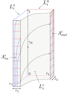
(a) Region $\mathbb{V}_{i}(r_{1},r_{2})$.

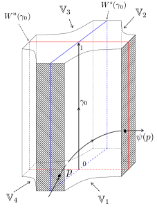
(b) Region $\mathbb{V}(r_{1},r_{2})$.

Figure 14: Cross-shaped neighbourhood.

Each of $\mathbb{V}_{i}$ is homeomorphic to a solid torus and its boundary is composed of five annuli:

$$(1)\ L^{s}_{i} =\ w^{s}_{i}\times\mathbb{R}/\mathbb{Z}$$

$$(2)\ L^{u}_{i} =\ w^{u}_{i}\times\mathbb{R}/\mathbb{Z}$$

$$(3)\ A_{in}^{i} =J_{in}^{i}\times\mathbb{R}/\mathbb{Z}$$

$$(4)\ A_{out}^{i} =J_{out}^{i}\times\mathbb{R}/\mathbb{Z}$$

$$(5)\ L^{c}_{i} =l_{i}\times\mathbb{R}/\mathbb{Z}.$$

The annuli $L_{i}^{s}$, $L_{i}^{u}$ and $L_{i}^{c}$ are tangent the vector field ${X_{(\lambda,n,p)}}$, being the first two contained in the stable and unstable manifolds of $\gamma_{0}$, respectively. The annuli $A_{in}^{i}$ and $A_{out}^{i}$ are the entrance and exit annuli, respectively. For $i=1$, this two annuli corresponds to the sets

$$A_{in}^{1} =\{(r_{1},r,z):0\leq r\leq r_{2},\ z\in\mathbb{R}/\mathbb{Z}\}$$

$$A_{out}^{1} =\{(r,r_{1},z):0\leq r\leq r_{2},\ z\in\mathbb{R}/\mathbb{Z}\}.$$

There is a diffeomorphism $\psi:A_{in}^{1}\backslash W^{s}(\gamma_{0})\to A_{out}^{1}\backslash W^{u}(\gamma_{0})$ of the form $\psi:p\mapsto q=\phi^{X_{(\lambda,n,p)}}(\tau(p),p),$ which sends each entrance point $p$ onto the point $q$ determined by the intersection $A_{out}^{1}\cap\mathcal{O}^{+}(p)$. The same holds for the other entrance-exit pair of annuli on the boundary.

Lemma 5.2 (See [25]).

Given $0<r_{2}<r_{1}<1$, the map $\psi:\{r_{1}\}\times(0,r_{2}]\times\mathbb{R}/\mathbb{Z}\to(0,r_{2}]\times\{r_{1}\}\times\mathbb{R}/\mathbb{Z}$ defined above satisfies that: For every $p=(r_{1},r,z)$, then $\psi(p)=(r,r_{1},z+\tau(p)/np)$ and $\tau(p)=\tau(r)=\frac{\log(r/r_{1})}{\log(\lambda)}$.

5.2.2 Singular orbit in the boundary of a Birkhoff section.

For each $\gamma\in\Gamma$, the local coordinates $\{\Pi_{i}:i=1,\dots,4\}$ given in (32) allow to construct a tubular neighbourhood $R=R(r_{1},r_{2})$ of the orbit $\gamma$ which depends on two parameters $0<r_{2}<r_{1}<1$, in the following way:

Cross-shaped neighbourhood.

For each $i=1,\dots,4$ consider the sets $\mathbb{V}_{i}(r_{1},r_{2})$ in $\mathbb{R}^{2}\times\mathbb{R}/\mathbb{Z}$ defined in (34) above. Let $0<r_{2}<r_{1}<1$ be such that each $\mathbb{V}_{i}(r_{1},r_{2})$ is contained in the image of $\Pi_{i}$. Define

$$R_{i}(r_{1},r_{2})=\overline{\left\{p\in W_{i}\backslash\gamma:\Pi_{i}(p)\in\mathbb{V}_{i}(r_{1},r_{2})\right\}}.$$ (36)

$$R(r_{1},r_{2})=\bigcup_{i}R_{i}(r_{1},r_{2}),i=1,\dots,4.$$ (37)

We say that $R=R(r_{1},r_{2})$ is a cross-shaped neighbourhood of $\gamma$.

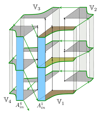
Figure 15: The neighbourhood $R(r_{1},r_{2})$ obtained glueing $\mathbb{V}_{i}(r_{1},r_{2})$.

Following remark 4.5 in section 4, we can describe the vector field $X_{\Gamma}$ on $R(r_{1},r_{2})\setminus\gamma$ in the following way: Consider the four pairs

$$\left(\mathbb{V}_{i}(r_{1},r_{2}),X_{(\lambda,n,p)}\right),\ i=1,\dots,4$$

consisting in the manifold $\mathbb{V}_{i}(r_{1},r_{2})$ equipped with the vector field $X_{(\lambda,n,p)}$ as in figure (14(a)). Then $\left(R(r_{1},r_{2})\setminus\gamma,X_{\Gamma}\right)$ is equivalent to the manifold obtained by glueing:

1. $\mathbb{V}_{1}$ with $\mathbb{V}_{2}$ along the boundary $L^{u}_{1}\to L^{u}_{2}$ with the map $(0,y,z)\mapsto(0,y,z)$,

2. $\mathbb{V}_{2}$ with $\mathbb{V}_{3}$ along the boundary $L^{s}_{2}\to L^{s}_{3}$ with the map $(x,0,z)\mapsto(x,0,z)$,

3. $\mathbb{V}_{3}$ with $\mathbb{V}_{4}$ along the boundary $L^{u}_{3}\to L^{u}_{4}$ with the map $(0,y,z)\mapsto(0,y,z)$,

4. $\mathbb{V}_{4}$ with $\mathbb{V}_{1}$ along the boundary $L^{s}_{4}\to L^{s}_{1}$ with the map $(0,y,z)\mapsto(0,y,z+\frac{m}{n})$.

In figure (15) we see this for $m=-1$, $n=2$ and $p=1$. The associated quotient space is a solid torus. Observe that the curve $0\times\mathbb{R}/\mathbb{Z}$ is a $n$-fold covering of its image under the quotient projection. In the complement of this curve, the vector field $X_{(\lambda,n,p)}$ is invariant by $z$-translations, so we get a well defined vector field on the quotient manifold.

The boundary $\partial R$ is decomposed in eight smooth annuli, four of them tangent to the vectorfield, two where $X_{\Gamma}$ is transverse and points inward the neighbourhood and two other where $X_{\Gamma}$ is transverse and points outward. Using the coordinates $\Pi_{i}$ we can identify the sets

$$\Pi_{i}:\partial R\cap R_{i}\to\partial\mathbb{V}\cap\mathbb{V}_{i}=A_{in}^{i}\cup L_{i}^{c}\cup A_{out}^{i}\subset\mathbb{D}_{i}\times\mathbb{R}/\mathbb{Z}.$$

In particular, the union $A_{in}^{1}\cup A_{in}^{4}$ is one of the eight annuli that forms $\partial R$, where the flow traverse inwardly. In coordinates (32), this two annuli correspond to the sets

$$A_{in}^{1} =\{(r_{1},r,z):0\leq r\leq r_{2},\ z\in\mathbb{R}/\mathbb{Z}\}$$

$$A_{in}^{4} =\{(r_{1},r,z):-r_{2}\leq r\leq 0,\ z\in\mathbb{R}/\mathbb{Z}\},$$

glued along the boundary $\{r_{1}\}\times 0\times\mathbb{R}/\mathbb{Z}$ with a vertical translation by $m/n$.

5.3 Construction of the smooth model.

In this subsection we construct the smooth model $(\psi_{t},N)$ associated to the topological Anosov flow $(\phi_{t},M)$. We recall the general assumption that $\Gamma$ consists in only one periodic orbit $\gamma$ and we set $n=n(\gamma,\Sigma)$, $m=m(\gamma,\Sigma)$ and $p=p(\gamma,\Sigma)$. Consider a smooth decreasing function $\rho:[0,1]\to[0,1]$ such that:

• $\rho(t)=1$, for $0\leq t\leq\frac{1}{3}$,

• $\rho^{\prime}(t)<0$, for $\frac{1}{3}<t<\frac{2}{3}$,

• $\rho(t)=0$, for $\frac{2}{3}\leq t\leq 1$.

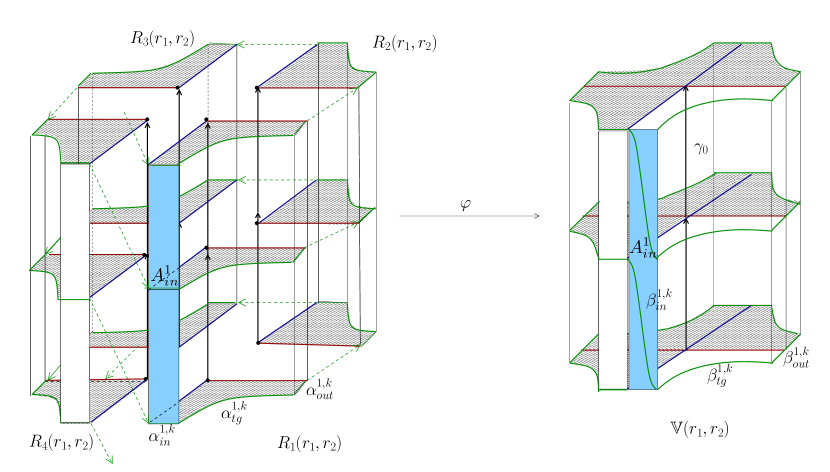
Figure 16: Glueing map $\varphi:\partial M_{R}(r_{1},r_{2})\to\mathbb{V}(r_{1},r_{2})$ with $m=-1$, $n=2$ and $p=1$.

Glueing map.

Let $\mathbb{V}(r_{1},r_{2})$ and $R(r_{1},r_{2})$ be the tubular neighbourhoods of $\gamma$ and $\gamma_{0}$ defined in (34)-(35) and (36)-(37), respectively. Let $M_{R}(r_{1},r_{2})\coloneqq M\backslash\textsl{int}(R(r_{1},r_{2}))$. Define $\varphi:\partial M_{R}(r_{1},r_{2})\to\partial\mathbb{V}(r_{1},r_{2})$ in the following way: For every $p\in\partial M_{R}(r_{1},r_{2})$ choose $1\leq i\leq 4$ such that $p$ belongs to the $i$-th quadrant and denote its coordinates by $(x,y,z)=\Pi_{i}(p)\in\mathbb{R}^{2}\times\mathbb{R}/\mathbb{Z}$. Then:

1. If $m=m(\gamma,\Sigma)<0$ then

   $$\varphi(p)=\left\{\begin{array}[]{cll}\left(x\ ,\ y\ ,\ z\right)&;\text{if }p\notin A_{in}^{1},\\ \left(r_{1}\ ,\ y\ ,\ z+\frac{|m|}{n}\rho\left(\frac{y}{r_{2}}\right)\right)&;\text{if }p\in A_{in}^{1}\text{ and }(r_{1},y,z)=\Pi_{1}(p).\end{array}\right.$$ (38)

2. If $m=m(\gamma,\Sigma)>0$ then

   $$\varphi(p)=\left\{\begin{array}[]{cll}\left(x\ ,\ y\ ,\ z\right)&;\text{if }p\notin A_{in}^{4},\\ \left(r_{1}\ ,\ y\ ,\ z+\frac{|m|}{n}\rho\left(-\frac{y}{r_{2}}\right)\right)&;\text{if }p\in A_{in}^{4}\text{ and }(r_{1},y,z)=\Pi_{4}(p).\end{array}\right.$$ (39)

In figure 16 we depict the map $\varphi$ in normal coordinates for the case $m=-1$, $n=2$, $p=1$. It is a twist map over the annulus $A_{in}^{1}$ and the identity on its complement.

Proposition 5.3.

For every couple of small parameters $0<r_{2}<r_{1}<1$, the map $\varphi$ given in (38)-(39) above is a well-defined diffeomorphism. Consider the manifold $N(r_{1},r_{2})=M_{R}(r_{1},r_{2})\sqcup_{\varphi}\mathbb{V}(r_{1},r_{2})$ obtained by glueing $M_{R}(r_{1},r_{2})$ and $\mathbb{V}(r_{1},r_{2})$ along their boundaries using $\varphi$. Then, there exists a smooth atlas $\mathcal{D}$ and a smooth vector field $Y$ on $N(r_{1},r_{2})$ such that:

1. The inclusion $\iota:M_{R}(r_{1},r_{2})\hookrightarrow N(r_{1},r_{2})$ is a diffeomorphism onto its image and $D\iota:X_{\Gamma}\mapsto Y$,

2. The inclusion $\iota:\mathbb{V}(r_{1},r_{2})\hookrightarrow N(r_{1},r_{2})$ is a diffeomorphism onto its image and $D\iota:X_{(\lambda,n,p)}\mapsto Y$.

We denote by $\psi_{t}:N(r_{1},r_{2})\to N(r_{1},r_{2})$ the flow generated by $Y$.

Notation: For notational simplicity we will set $M_{0}=M_{R}(r_{1},r_{2})$ and $M_{1}=\mathbb{V}(r_{1},r_{2})$, and for each $j=0,1$ we denote by $X_{j}$ the corresponding vector field. We denote by $N=M_{0}\sqcup_{\varphi}M_{1}$ and by $\iota_{j}:M_{j}\to N$ the natural inclusion maps. The two components are glued along the subset $M_{0}\cap M_{1}\simeq\partial M_{0}\simeq\partial M_{1}$ that is homeomorphic to a two dimensional torus.

Proof.

In coordinates (32) the map $\varphi$ consists in apply a twist map, supported on the annuli $A_{in}^{1}$ or $A_{in}^{4}$ depending on the signature of the linking number. This assumption will be important in 5.5 for the purpose of constructing a Birkhoff section. Along this proof we will stay in the case $m<0$ and $\textsl{supp}(\varphi)=A_{in}^{1}$, being analogous the other one.

The partition of the neighbourhood $W$ in quadrants decomposes $\partial R$ in four regions, individually homeomorphic to the annulus. To show that $\varphi$ is well-defined we have to check its definition along the intersections of these four regions. It is well-defined over the intersections $A_{out}^{1}\cap A_{out}^{2}$, $A_{in}^{2}\cap A_{in}^{3}$ and $A_{out}^{3}\cap A_{out}^{4}$ because $\Pi_{i+1}\circ\Pi_{i}^{-1}=id$, for $i=1,2,3$. To check that it is well-defined on the intersection $A_{in}^{4}\cap A_{in}^{1}$ let $p$ be a point in this intersection with coordinates $\Pi_{4}(p)=(r_{1},0,z)$ and $\Pi_{1}(p)=(r_{1},0,z+m/n)$. Then applying (38) we have

$$\text{for}\ p\in A_{in}^{4}, \ \varphi(p)=id\circ\Pi_{4}(p)=(r_{1},0,z),$$

$$\text{for}\ p\in A_{in}^{1}, \ \varphi(p)=\Pi_{1}(p)+(0,0,|m|/n)=(r_{1},0,z).$$

Thus $\varphi$ is a well-defined bijection between the boundary of $M_{0}$ and the boundary of $M_{1}$, and since the function $\rho$ above is constant in a neighbourhood of $0$, we deduce that $\varphi$ is a diffeomorphism.

The quotient space $N=M_{0}\sqcup_{\varphi}M_{1}$ is then a $3$-manifold, and since each $M_{i}$ is smooth there is a smooth atlas defined over $N\backslash(M_{0}\cap M_{1})$, induced by the inclusions $\iota_{j}:\textsl{int}(M_{j})\hookrightarrow N$. To extend this smooth atlas along $M_{0}\cap M_{1}$ it suffices to provide a family

$$\left\{\Phi_{p}:T_{p}M_{0}\to T_{\varphi(p)}M_{1},p\in\partial M_{0}\right\}$$ (40)

satisfying that

1. $\Phi_{p}:T_{p}M_{0}\to T_{\varphi(p)}M_{1}$ is a linear isomorphism, $\forall\ p\in\partial M_{0}$,

2. $\Phi_{p}|_{T_{p}\partial M_{0}}=D\varphi$,

3. the map $p\mapsto\Phi_{p}$ varies smoothly.

If in addition we want that the vector fields $X_{j}$, $j=1,2$ match together along the boundary, we need that

• $\Phi_{p}:X_{0}(p)\mapsto X_{1}(\varphi(p))$, $\forall\ p\in\partial M_{0}$.

Now, choose a point $p\in\partial M_{0}$ belonging to the $i$-th quadrant. If $p\notin A_{in}^{1}$, since $\varphi\circ\Pi_{i}^{-1}=id$ in a neighbourhood of $p$, $D\Pi_{i}:X_{0}\mapsto X_{(\lambda,n,p)}$ and $(M_{1},X_{1})=(\mathbb{V},X_{(\lambda,n,p)})$, we see that

$$\Phi_{p}:T_{p}M_{0}\to T_{\varphi(p)}M_{1}\text{ given by }\Phi_{p}\circ D\Pi_{i}^{-1}=id_{\mathbb{R}^{3}}$$ (41)

satisfies (i)-(iv) above. If $p\in A_{in}^{1}$, since the vector field $X_{0}$ is transverse to the boundary of $M_{0}$ along the annulus $A^{1}_{in}$ and points outward, and $X_{1}$ is transverse to the boundary of $M_{1}$ along $\varphi(A_{in}^{1})$ and points inward, then

$$\Phi_{p}:T_{p}M_{0}\to T_{\varphi(p)}M_{1}\text{ given by }\Phi_{p}|_{T_{p}\partial M_{0}}=D\varphi(p)\text{ and }\Phi_{p}(X_{0}(p))=X_{1}(p)$$ (42)

satisfies the desired properties (i)-(iv). Since $\varphi$ coincides with a vertical translation near the boundary components of $A_{in}^{1}$ and $X_{(\lambda,n,p)}$ is invariant by these translations, then the transformation in (42) satisfies $\Phi_{p}\circ D\Pi_{1}^{-1}=id$ for points $p$ near $\partial A_{in}^{1}$, so it is compatible with (41) above. For more details on this proof see [25], or [14], [15], [7] for more details on how to glue vector fields along the boundary. ∎

5.3.1 The action of the flow $\psi_{t}:N\to N$.

The action of the flow $\psi_{t}$ on a point $p$ in the manifold $N=M_{0}\sqcup_{\varphi}M_{1}$ can be described as an alternated composition of integral curves of $X_{j}$ on each component $M_{j}$ and the glueing map $\varphi$. The positive orbit of a typical point $p$ starting in $\textsl{int}(M_{0})$ will follow the $\phi_{t}^{0}$-trajectory in $M_{0}$ until the first time $t_{1}>0$ it reaches $\partial M_{0}$ in a point $p_{1}=\phi_{t_{1}}^{0}(p)$. Then, $p_{1}$ is identified with $\varphi(p_{1})\in\partial M_{1}$ and the orbit switches to the component $M_{1}$, concatenating with the $\phi_{t}^{1}$-trajectory starting on the point $\varphi(p_{1})$. The same holds for typical points starting in $M_{1}$, but using $\varphi^{-1}$ for traversing from $M_{1}$ to $M_{0}$ instead. We remark that there exists a constant $T>0$ such that, for both $j=0,1$, the quantity

$$\min\left\{t>0:\exists\ p\in\partial M_{j}\text{ s.t. }\phi_{t}^{j}(p)\in\partial M_{j}\text{ and }\phi_{s}^{j}(p)\in\textsl{int}(M_{j}),\forall 0<s<t\right\}$$

is greater that $T$. It follows that:

Lemma 5.4 (See [25]).

Given $p\in\textsl{int}(M_{0})$ and $t\geq 0$ such that $\psi_{t}(p)\in\textsl{int}(M_{0})$, it exist $0<t_{1},\dots,t_{l+1}<t$ and $0<s_{1},\dots,s_{l}<t$ satisfying that $t_{k}\geq T$ for $k=2,\dots,l$, $s_{k}\geq T$ for $k=1,\dots,l$, their sum is $\sum_{k=0}^{l}t_{k}+\sum_{k=1}^{l}s_{k}=t$ and

$$\psi_{t}(p)=\phi_{t_{l+1}}^{0}\left(\varphi^{-1}\cdot\phi_{s_{l}}^{1}\cdot\varphi\right)\cdots\left(\varphi^{-1}\cdot\phi_{s_{2}}^{1}\cdot\varphi\right)\cdot\phi_{t_{2}}^{0}\cdot\left(\varphi^{-1}\cdot\phi_{s_{1}}^{1}\cdot\varphi\right)\cdot\phi_{t_{1}}^{0}(p).$$

The set of the $s_{i}$’s may be empty (l=0) and in that case $t_{1}=t$. Analogue formulations holds for $\psi_{t}$-orbit segments starting and ending in any combination of components $M_{j}$, $j=0,1$.

We describe now the derivative action $D\psi_{t}:TN\to TN$ on the tangent bundle. Recall that on each component $(M_{j},X_{j})$, $j=0,1$, there is a splitting $TM_{j}=E^{s}_{j}\oplus E^{c}_{j}\oplus E^{u}_{j}$ and a Riemannian metric $|\cdot|_{j}$ (cf. (33) for $(M_{0},X_{0})=(M_{\Gamma},X_{\Gamma})$ and remark 5.1 for $(M_{1},X_{1})=(\mathbb{V},X_{(\lambda,n,p)})$), that is invariant by $D\phi_{t}^{j}(p)$ (for every $p\in M_{j}$ and $t\in\mathbb{R}$ such that the $\phi_{t}^{j}$-orbit segment between $p$ and $\phi_{t}^{j}(p)$ is entirely contained in $M_{j}$) and uniformly hyperbolic with contraction rate $0<\lambda<1$, where $E^{s}_{j}$ is the contracting bundle, $E^{u}_{j}$ the expanding bundle and $E^{c}_{j}=\textsl{span}\{X_{j}\}$.

Framing on TN.

To study the action of $D\psi_{t}$ on $TN$ we define a (non-continuous) splitting by $T_{p}N=H^{s}(p)\oplus H^{c}(p)\oplus H^{u}(p)=$

$$\left\{\begin{array}[]{lll}E^{s}_{1}(p)\oplus E^{c}_{1}(p)\oplus E^{u}_{1}(p),\ \text{if}\ p\in\textsl{int}(M_{1}),\\ E^{s}_{0}(p)\oplus E^{c}_{0}(p)\oplus E^{u}_{0}(p),\ \text{if}\ p\in N\setminus\textsl{int}(M_{1}),\end{array}\right.$$ (45)

Remark 5.5.

We can see how does $E^{s}_{0}\oplus E^{c}_{0}\oplus E^{u}_{0}$ matches $E^{s}_{1}\oplus E^{c}_{1}\oplus E^{u}_{1}$ along $M_{0}\cap M_{1}$ using the identifications $\Phi_{p}:T_{p}M_{0}\to T_{\varphi(p)}M_{1}$ given in (40), (41), (42). For every $p\in\partial M_{0}$ the map $\Phi_{p}$ sends $X_{0}(p)\mapsto X_{1}(\varphi(p))$, so it follows that the bundle $H^{c}=\textsl{span}\{Y\}$ is continuous. If $p\notin A_{in}^{1}$ then by (33), (41) and 3. on remark 5.1, we obtain that $\Phi_{p}$ sends $E^{s}_{0}(p)\mapsto E^{s}_{1}(\varphi(p))$ and $E^{u}_{0}(p)\mapsto E^{u}_{1}(\varphi(p))$, obtaining continuity of the decomposition (45) in $p$. Nevertheless, for points $p\in A_{in}^{1}$ the two decompositions $E^{s}_{0}(p)\oplus E^{c}_{0}(p)\oplus E^{u}_{0}(p)$ and $E^{s}_{1}(\varphi(p))\oplus E^{c}_{1}(\varphi(p))\oplus E^{u}_{1}(\varphi(p))$ will not agree via $\Phi_{p}$ in general, so the framing (45) above may be non-continuous in $p$.

Lemma 5.6.

Given $p\in N$ and $t>0$, there exist $0<t_{1},\dots,t_{l+1}<t$ satisfying $t_{k}\geq T$ for $k=2,\dots,l$ and points $p_{1},\dots,p_{l}\in A_{in}^{1}$ (empty in case $l=0$) such that $D\psi_{t}:T_{p}N\to T_{\psi_{t}(p)}N$ is an iterated composition of the form:

$$D\psi_{t}(p)=\Psi_{t_{l+1}}\circ\Phi_{p_{l}}\circ\Psi_{t_{l}}\cdots\circ\Phi_{p_{2}}\circ\Psi_{t_{2}}\circ\Phi_{p_{1}}\circ\Psi_{t_{1}}(p),$$ (46)

where the transformations $\Psi_{\tau}$ and $\Phi_{p}$ are the following:

1. $\Psi_{\tau}$ denotes the application $T_{p}N\to T_{\psi_{\tau}(p)}N$, defined for all the couples $(\tau,p)$ satisfying that $[p,\psi_{\tau}(p)]\cap A_{in}^{1}=\emptyset$ by the expression:

   $$\Psi_{t}:aY(p)+be_{s}(p)+ce_{u}(p)\mapsto aY(\psi_{\tau}(p))+\lambda^{t}be_{s}(\psi_{\tau}(p))+\lambda^{-t}ce_{u}(\psi_{\tau}(p)),$$ (47)

   where $\{Y,e_{s},e_{u}\}$ is a continuous frame along the curve $[p,\psi_{\tau}(p)]$ s.t. $e_{s}(\psi_{\theta}(p))\in H^{s}(\psi_{\theta}(p))$ and $e_{u}(\psi_{\theta}(p))\in H^{u}(\psi_{\theta}(p))$ are unitary vectors, for every $0\leq\theta\leq\tau$.

2. $\Phi_{p}:T_{p}M_{0}\to T_{\varphi(p)}M_{1}$ are the transformations defined in (42) for $p\in A_{in}^{1}$. Given $p\in A_{in}^{1}$ with coordinates $\Pi_{1}(p)=(r_{1},r,z)$, $0\leq r\leq r_{2}$, consider two basis

   $$\mathcal{B}_{0}=\{X_{0}(p),e_{0}^{s}(p),e_{0}^{u}(p)\}\ \text{and}\ \mathcal{B}_{1}=\{X_{1}(\varphi(p)),e_{1}^{s}(\varphi(p)),e_{1}^{u}(\varphi(p))\}$$

   of $T_{p}M_{0}$ and $T_{\varphi(p)}M_{1}$ respectively, where the $e_{j}^{s}$, $e_{j}^{u}$ are unitary vectors contained the spaces $E_{j}^{s}$, $E_{j}^{u}$ and oriented as in 4 below. Then

   $$_{\mathcal{B}_{1}}\left(\Phi_{p}\right)_{\mathcal{B}_{0}}=\begin{pmatrix}1&-\frac{\kappa(r)npr}{r_{1}r_{2}}&-\frac{\kappa(r)np}{r_{2}}\\ 0&\kappa(r)np\log(\lambda)\frac{r}{r_{2}}+1&\kappa(r)np\log(\lambda)\frac{r_{1}}{r_{2}}\\ 0&-\kappa(r)np\log(\lambda)\frac{r^{2}}{r_{1}r_{2}}&-\kappa(r)np\log(\lambda)\frac{r}{r_{2}}+1\end{pmatrix}$$ (48)

   $\text{where}\ \kappa(r)=\frac{|m|}{n}\left|\rho^{\prime}(r/r_{2})\right|.$

Proof.

The expression in (46) follows lemma 5.4 by taking derivatives and using that, when switching from one component $M_{j}$ to the other, the tangent spaces are identified with the transformations (40)-(41)-(42). For $k=1,\dots,l$ denote by $p_{k}=\psi_{t_{k}+s_{k-1}}(p_{k-1})$ and $q_{k}=\psi_{s_{k}}(p_{k})$, so the orbit of $p$ switches from $M_{0}$ to $M_{1}$ on the points $p_{k}$, and from $M_{1}$ to $M_{0}$ on the points $q_{k}$. We obtain that

$$D\psi_{t}(p)=D\phi_{t_{l+1}}^{0}\cdot\Phi_{q_{l}}\cdot D\phi_{s_{l}}^{1}\cdot\Phi_{p_{l}}\cdots\Phi_{q_{1}}\cdot D\phi_{s_{1}}^{1}\cdot\Phi_{p_{1}}\cdot D\phi_{t_{1}}^{0}(p).$$

Since the points $q_{k}$ are not contained in the support $A_{in}^{1}$ of the glueing map $\varphi$, then $\Phi_{q_{k}}=id$ by (41) and we can reduce the previous expression by only considering the points $p_{k}$ (and corresponding times $t_{k}$) where the orbit segment $[p,\psi_{t}(p)]$ intersects $A_{in}^{1}$. Since each transformation $D\phi_{\tau}^{j}$ acts on $TM_{j}$ in the form specified in (47), we deduce (46).

To show (48), consider $p\in A_{in}^{1}$ with coordinates $\Pi_{1}(p)=(r_{1},r,z)$, $0\leq r\leq r_{2}$. Consider the basis of $\mathbb{R}^{3}$ given by

$$\{e_{1}=(1,0,0),e_{2}=(0,1,0),e_{3}=(0,0,1)\}.$$

Then, by (33) and 3. on 5.1 it follows that $\mathcal{B}_{0}=\{X_{(\lambda,n,p)}(\Pi_{1}(p)),e_{1},e_{2}\}$ and $\mathcal{B}_{1}=\{X_{(\lambda,n,p)}(\varphi(p)),$ $e_{1},e_{2}\}$ are basis satisfying the hypothesis above. Thus, the matrix (48) is the expression in these basis of $\Phi_{p}\circ D\Pi_{1}^{-1}:\mathbb{R}^{3}\to\mathbb{R}^{3}$. Now, since $\Phi_{p}$ sends $:X_{(\lambda,n,p)}(\Pi_{1}(p))\mapsto X_{(\lambda,n,p)}(\varphi(p))$ and coincides with $D\varphi$ on $TA_{in}^{1}=0\times\mathbb{R}\times\mathbb{R}$, in the basis $\mathcal{C}=\{X_{(\lambda,n,p)},e_{2},e_{3}\}$ we have that

$$_{\mathcal{C}}\left(\Phi_{p}\right)_{\mathcal{C}}=\begin{pmatrix}1&0&0\\ 0&1&0\\ 0&-\frac{\kappa(r)}{r_{2}}&1\end{pmatrix},\text{ where }\kappa(r)=\frac{|m|}{n}\left|\rho^{\prime}(r/r_{2})\right|.$$ (49)

The expression (48) is finally obtained by applying a change of basis between $\mathcal{C}$ and $\mathcal{B}_{j}$.

∎

5.3.2 Invariant measure.

Proposition 5.7.

The flow $\psi_{t}:N\to N$ in proposition 5.3 preserves a smooth volume form.

Proof.

To prove this we will define a smooth volume form $\omega_{i}$ on each $M_{i}$, $i=0,1$, invariant by the action of $\phi_{t}^{i}$, and we will see that they match together along $M_{0}\cap M_{1}$ under the glueing map $\varphi$.

For each $p\in M_{0}$ consider a positively oriented basis $\{X_{0}(p),e_{s}^{0}(p),e_{u}^{0}(p)\}$ of $T_{p}M_{0}$, according to the decomposition $E_{0}^{s}(p)\oplus E^{c}_{0}(p)\oplus E^{u}_{0}(p)$, and such that $|e_{s}^{0}(p)|_{0}=|e_{u}^{0}(p)|_{0}=1$. Define a volume form $\omega_{0}$ in $M_{0}$ by the expression $\omega_{0}(p)=dX_{0}(p)\wedge de_{s}^{0}(p)\wedge e_{u}^{0}(p)$. Since by the construction on 4 the splitting $TM_{0}=E^{s}_{0}\oplus E^{c}_{0}\oplus E^{u}_{0}$ is smooth then $\omega_{0}$ is a smooth volume form on $M_{0}$, and from (47) it follows that:

$$\left(D\phi_{t}^{0}\right)^{*}\omega_{0}(p) =dX_{0}(\psi_{t}(p))\wedge\lambda^{t}\cdot de_{s}^{0}(\psi_{t}(p))\wedge\lambda^{-t}\cdot de_{u}^{0}(\psi_{t}(p))$$

$$=dX_{0}(p)\wedge de_{s}^{0}(p)\wedge de_{u}^{0}(p)=\omega_{0}(p),$$

for every $p\in M_{0}$ and $t\geq 0$ such that $[p,\phi_{t}^{0}(p)]$ is contained in $M_{0}$.

For each point $p=(x,y,z)\in M_{1}=\mathbb{V}(r_{1},r_{2})$ consider the basis of $T_{p}M_{1}$ given by $\{X_{1}(p),e_{1},e_{2}\}$, where $e_{1}=(1,0,0)$ and $e_{2}=(0,1,0)$. Define $\omega_{1}(p)=dX_{1}(p)\wedge dx\wedge dy$. Then, this is a smooth volume form and by remark 5.1 we have

$$\left(D\phi_{t}^{1}\right)^{*}\omega_{1}(p)=dX_{0}(\psi_{t}(p))\wedge\lambda^{t}\cdot dx\wedge\lambda^{-t}\cdot dy=dX_{0}(p)\wedge dx\wedge dy=\omega_{1}(p),$$

for every $p\in M_{1}$ and $t\geq 0$ such that $[p,\phi_{t}^{1}(p)]$ is contained in $M_{1}$.

Finally, observe that by (48), for every $p\in\partial M_{0}$ the transformation $\Phi_{p}:T_{p}M_{0}\to T_{\varphi(p)}M_{1}$ has determinant $\det(\Phi_{q})=1$ in the basis $\{X_{i},e_{s}^{i},e_{u}^{i}\}$. Thus

$$\left(\Phi_{p}\right)^{*}\omega_{1}(p)=\det(\Phi_{q})\cdot\omega_{0}(p)=\omega_{0}(p),$$

for every $p\in\partial M_{0}$. From the three expressions above and the decomposition of $D\psi_{t}$ in products of $\Psi_{t}$ and $\Phi_{q}$ given in lemma 5.6, we conclude that the $3$-form $\omega$ on $N=M_{0}\sqcup_{\varphi}M_{1}$ defined by $\omega(p)=\omega_{i}(p)$ for $p\in M_{i}$ is a well defined smooth volume form satisfying $\psi_{t}^{*}(\omega)=\omega$. ∎

5.4 Hyperbolicity.

Proposition 5.8.

If $0<r_{2}<r_{1}<1$ are sufficiently small, then the flow $\psi_{t}:N(r_{1},r_{2})\to N(r_{1},r_{2})$ constructed in proposition 5.3 is Anosov.

The proof of proposition 5.8 proceeds by applying the cone field criterion; see [18] or [14], [15] for a precise statement. We divide it in two propositions. In proposition 5.9 we show that $D\psi_{t}:TN\to TN$ preserves a pair of center-stable and center-unstable 2-dimensional plane fields by application of this criterion. Then, in proposition 5.13 we apply the same criterion inside the center-stable and center-unstable planes to conclude the existence of a hyperbolic splitting preserved by $D\psi_{t}$.

In the definition of $\varphi$ in (38) and (39) there is an auxiliary smooth function $\rho$ and two parameters $0<r_{2}<r_{1}<1$. The maximum size of these real parameters depend on the charts $\Pi_{i}$, but they can be chosen arbitrarily small. We assume from now on that $\rho$ is fixed and we will adjust the parameters $r_{1},r_{2}$ to satisfy the proposition.

5.4.1 Existence of the center-stable and center-unstable invariant distributions.

Proposition 5.9.

There exist two continuous plane distributions $F^{cs}$ and $F^{cu}$ in the tangent bundle $TN$ satisfying that:

1. $D\psi_{t}(p)\left(F^{cu}(p)\right)=F^{cu}(\psi_{t}(p))$ and $D\psi_{t}(p)\left(F^{cs}(p)\right)=F^{cs}(\psi_{t}(p))$, for every $p\in N$ and $t\in\mathbb{R}$;

2. $F^{cs}(p)\cap F^{cu}(p)=H^{c}(p)=\textsl{span}\{Y(p)\}$, for every $p\in N$;

3. There exists constants $L>0$ and $\mu>1$ such that

   $$\|D\psi_{t}(p)\cdot v\ \|\geq L\mu^{t}\|v\|,\ \forall\ p\in N,\ v\in F^{cu}(p)\backslash H^{c}(p),\ t\geq 0,$$

   $$\|D\psi_{-t}(p)\cdot v\|\geq L\mu^{t}\|v\|,\ \forall\ p\in N,\ v\in F^{cs}(p)\backslash H^{c}(p),\ t\geq 0.$$

To prove 5.9 define:

Stable and unstable slopes.

Given a point $p\in N$ consider a positively oriented basis of $T_{p}N$ of the form $\{Y(p),e_{s}(p),e_{u}(p)\}$, where $e_{s}(p)$ and $e_{u}(p)$ are unitary vectors contained in the spaces $H^{s}(p)$ and $H^{u}(p)$ of the decomposition (45), respectively. Given a vector $v=aY(p)+be_{s}(p)+ce_{u}(p)$ in $T_{p}N$ we define its $u$-slope and $s$-slope respectively as

$$\Delta_{u}(v)=\frac{b}{c}\ \text{and}\ \Delta_{s}(v)=\frac{c}{b}.$$

There are two possibilities for choosing a positive basis as before, but the slope is unchanged by switching this election, so the $u$,$s$-slopes are well defined.

Cone distributions

Given two real numbers that $-\infty<\delta_{0}<\delta_{1}<+\infty$ we define two cones

$$C^{cu}(p;\delta_{0},\delta_{1})=\left\{v\in T_{p}N\ :\ \delta_{0}\leq\Delta_{u}\leq\delta_{1}\right\}$$

$$C^{cs}(p;\delta_{0},\delta_{1})=\left\{v\in T_{p}N\ :\ \delta_{0}\leq\Delta_{s}\leq\delta_{1}\right\}.$$

At each point $p$ this is a pair of $2$-dimensional cones, with axis determined by the vector $Y(p)$.

Norm in $TN$.

For every vector $v=aY(p)+be_{s}(p)+ce_{u}(p)$ in $T_{p}N$ we define its norm by the formula $\|v\|=\sqrt{a^{2}+b^{2}+c^{2}}$. This norm comes from a Riemannian metric defined by setting that $\{Y(p),e_{s}(p),e_{u}(p)\}$ is an orthonormal basis at each $p\in N$.

We will show that for some adequate slope values $\delta_{0}^{u},\delta_{1}^{u}$ and $\delta_{0}^{s},\delta_{1}^{s}$ there is a pair of $cu$- and $cs$-cones satisfying the cone field criterion under the action of $D\psi_{t}:TN\to TN$. We remark that the slope functions, the cone distributions $p\mapsto C^{cu}(p;\delta_{0}^{u},\delta_{1}^{u})$ and $p\mapsto C^{cs}(p;\delta_{0}^{s},\delta_{1}^{s})$, and the Riemannian metric defined above are not continuous as functions of $p\in N$. This is due to the discontinuities of the splitting (45) over the set $A_{in}^{1}$. Nevertheless, this posses no obstructions for applying the criterion. The criterion consists in checking the following three statements:

Lemma 5.10.

Let $\delta_{0}^{u},\delta_{1}^{u},\delta_{0}^{s},\delta_{1}^{s}:N\to\mathbb{R}$ be the quantities defined in (53) below. If $0<r_{2}<r_{1}<1$ are sufficiently small, then there exists $T>0$ such that: For every $p\in N$,

$$D\psi_{t}\left(C^{cu}\left(p\ ;\ \delta_{0}^{u},\delta_{1}^{u}\ \right)\right)\subset C^{cu}\left(\psi_{t}(p)\ ;\ \delta_{0}^{u},\delta_{1}^{u}\ \right),\ \forall\ t\geq T,$$

$$D\psi_{-t}\left(C^{cs}\left(p\ ;\ \delta_{0}^{s},\delta_{1}^{s}\ \right)\right)\subset C^{cs}(\psi_{-t}(p)\ ;\ \delta_{0}^{s},\delta_{1}^{s}\ )),\ \forall\ t\geq T.$$

Lemma 5.11.

For the parameters $0<r_{2}<r_{1}<1$ given in the previous lemma, it is satisfied the following: There exists a constant $L_{0}>0$ such that, for every $p\in N$ and every $t\geq 0$ then

$$\left|\ \Delta_{u}(D\psi_{t}(p)\cdot v_{2})-\Delta_{u}(D\psi_{t}(p)\cdot v_{1})\ \right|\leq\lambda^{2t}L_{0},\ \forall\ v_{1},v_{2}\in C^{cu}(p;\delta_{0}^{u},\delta_{1}^{u}),$$

$$\left|\Delta_{s}(D\psi_{-t}(p)\cdot v_{2})-\Delta_{s}(D\psi_{-t}(p)\cdot v_{1})\right|\leq\lambda^{2t}L_{0},\ \forall\ v_{1},v_{2}\in C^{cs}(p;\delta_{0}^{s},\delta_{1}^{s}).$$

Lemma 5.12.

By shrinking the parameters $0<r_{2}<r_{1}<1$ of the previous lemmas if necessary, it is satisfied that: There exist constants $L>0$ and $\mu>1$ such that, for every $p\in N$ and every $t\geq 0$ then

$$\left\|D\psi_{t}(p)\cdot v\ \right\|\geq L\mu^{t}\|v\|,\ \forall\ v\in C^{cu}(p;\delta_{0}^{u},\delta_{1}^{u})\setminus H^{c}(p),$$

$$\left\|D\psi_{-t}(p)\cdot v\right\|\geq L\mu^{t}\|v\|,\ \forall\ v\in C^{cu}(p;\delta_{0}^{s},\delta_{1}^{s})\setminus H^{c}(p).$$

Proof of prop. 5.9..

Define

$$F^{cu}(p)=\bigcap_{k\geq 0}D\psi_{kT}\left(\ C^{cu}(\ \psi_{-kT}(p)\ ;\ \delta_{0}^{u},\delta_{1}^{u}\ )\ \right),$$

$$F^{cs}(p)=\bigcap_{k\geq 0}D\psi_{-kT}\left(\ C^{cu}(\ \psi_{kT}(p)\ ;\delta_{0}^{u},\delta_{1}^{u}\ )\ \right).$$

This is a pair of $2$-dimensional cones (decreasing intersection of cones by lemma 5.10) contained in $T_{p}N$. The slope function $\Delta_{u}$ allows to identify each cone $C^{cu}(p;\delta_{0}^{u},\delta_{1}^{u})$ with the closed interval $[\delta_{0}^{u},\delta_{1}^{u}]\subset\mathbb{R}$. By lemmas 5.10 and 5.11, $F^{cu}(p)$ corresponds with a nested intersection of compact segments whose diameter tends to zero, so it is a non-empty cone that in fact reduces to a two dimensional plane. The same considerations apply for $F^{cs}(p)$.

Now, by lemma 5.12 we deduce the expansion/contraction property stated in 3. of proposition 5.9 for each $F^{cu}$ and $F^{cs}$. Since $|D\psi_{t}(p)\cdot v|\to+\infty$ for vectors $v\in F^{cu}(p)\backslash H^{c}(p)$ and $|D\psi_{t}(p)\cdot w|\to 0$ for vectors $w\in F^{cs}(p)\backslash H^{c}(p)$ (and $t\geq 0$) then $F^{cu}(p)\cap F^{cs}(p)=\textsl{span}\{Y(p)\}$. Finally, observe that if a pair of planes $E^{cs}(p)$ and $E^{cu}(p)$ in $T_{p}N$ satisfies 3. in 5.9, then $E^{cs}(p)=F^{cs}(p)$ and $E^{cu}(p)=F^{cu}(p)$. In particular, we obtain the invariance

$$D\psi_{t}:F^{cu}(p)\mapsto F^{cu}(\psi_{t}(p)),\ \ D\psi_{t}:F^{cu}(p)\mapsto F^{cs}(\psi_{t}(p)),\ \ \forall\ t\in\mathbb{R}.$$

The continuity of the bundles $p\mapsto F^{cu}(p)$ and $p\mapsto F^{cs}(p)$ is automatic: this property is true for every pair of invariant plane bundles satisfying 1., 2. and 3. in proposition 5.9, see . ∎

We proceed now to the proof of lemmas 5.10, 5.11 and 5.12.

Action on the $su$-bundle.

To study the action of $D\psi_{t}$ on cone distributions consider the vector bundle $\bar{H}^{su}\to N$ defined by the quotient $\bar{H}^{su}(p)\coloneqq T_{p}N/H^{c}(p),\ \forall\ p\in N,$ which carries an induced action of $D\psi_{t}$. There is a decomposition of this bundle of the form $\bar{H}^{su}=\bar{H}^{s}\oplus\bar{H}^{u}$, induced form $TN=H^{s}\oplus H^{c}\oplus H^{u}$. By lemma 5.6 the action of $\psi_{t}$ on $\bar{H}^{su}$ is an alternated composition of transformations of the form $\Psi_{t}$ and $\Phi_{p}$. For every $p\in N$ let $\{\bar{e}_{s}(p),\bar{e}_{u}(p)\}$ be a positive basis of $\bar{H}^{su}$ induced from two unitary vectors in $H^{s}$ and $H^{u}$. We have that:

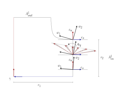
Figure 17: The map $\Phi_{p}$ in $su$-coordinates.

1. If $p\notin A_{in}^{1}$ and $t>0$ satisfies that $[p,\psi_{t}(p)]\cap A_{in}^{1}=\emptyset$, then the matrix associated to the action $D\psi_{t}(p)$ on the $su$-bundle, in the basis $\{\bar{e}_{s},\bar{e}_{u}\}$, is given by

   $$\left(\Psi_{t}\right)_{su}=\begin{pmatrix}\lambda^{t}&0\\ 0&\lambda^{-t}\end{pmatrix}.$$ (50)

2. Let $p\in A_{in}^{1}$ with coordinates $\Pi_{1}(p)=(r_{1},r,s)$. By (48) in lemma 5.6 we see that that the action of $\Phi_{p}$ in the $su$-bundle, in the basis $\{\bar{e}_{s},\bar{e}_{u}\}$, is given by the matrix

   $$\left(\Phi_{p}\right)_{su}=\begin{pmatrix}K(r,r_{2})+1&K(r,r_{2})\frac{r_{1}}{r}\\ -K(r,r_{2})\frac{r}{r_{1}}&-K(r,r_{2})+1\end{pmatrix},$$ (51)

   where $K(r,r_{2})=-(cte)\cdot|\rho^{\prime}(r/r_{2})|\frac{r}{r_{2}}$ and $(cte)=p|m||\log(\lambda)|$. Remark that $K$ is a non-positive function. Thus, we obtain a family of transformations parametrized over $0\leq r\leq r_{2}$. Observe that $\Phi_{p}$ is non-trivial just for points $p=(r_{1},r,s)$ with $\frac{r_{2}}{3}\leq r\leq\frac{2r_{2}}{3}$ due to the definition of $\rho:[0,1]\to\mathbb{R}$. Since (51) has determinant equal to one and trace equal to two, it has a double eigenvalue equal to one. The vector $\bar{w}_{1}=-\bar{e}_{s}+\frac{r}{r_{1}}\bar{e}_{u}$ is an eigenvector for this matrix in the $\bar{H}^{su}$ plane. Consider the vector $\bar{w}_{2}=\frac{r}{r_{1}}\bar{e}_{s}+\bar{e}_{u}$. In the orthogonal basis $\{\bar{w}_{1},\bar{w}_{2}\}$ the transformation (51) takes the form

   $$\left(\Phi_{p}\right)_{\{\bar{w}_{1},\bar{w}_{2}\}}=\begin{pmatrix}1&\eta(r)\frac{r_{1}}{r_{2}}\\ 0&1\end{pmatrix}$$ (52)

   for some continuous function $\eta:[0,r_{2}]\to[0,\infty)$ with support in $[\frac{r_{2}}{3},\frac{2r_{2}}{3}]$. We illustrate the action of the matrix (51) in figure 17.

Choice of slopes.

Define

$$\delta_{0}^{u}=-\frac{3r_{1}}{r_{2}},\ \delta_{1}^{u}=\frac{r_{2}}{3r_{1}}\ \text{ and }\ \delta_{0}^{s}=-\frac{3r_{1}}{2r_{2}},\ \delta_{1}^{s}=\frac{2r_{2}}{3r_{1}}.$$ (53)

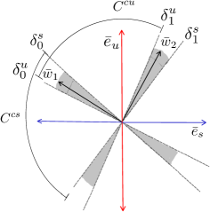
(a)  

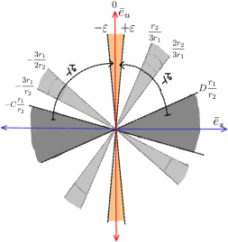
(b)  

Figure 18: Cones in the $su$-plane

Proof of lemma 5.10.

We make the proof for the $cu$-case, being analogous the other one. We will use the decomposition of $D\psi_{t}$ as product of matrices (50) and (51) acting on $\bar{H}^{su}$ explained above. We study first how the transformations $\Phi_{q}$ given in (51) act on the cones $C^{cu}(q;\delta_{0}^{u},\delta_{1}^{u})$, for every point $q=(r_{1},r,s)\in A_{in}^{1},\ 0\leq r\leq r_{2}$. Recall from (52) above that each non-trivial $\Phi_{q}$ has an eigenvector $\bar{w}_{1}(q)$ (double eigenvalue equal to $1$) whose $u$-slope is bounded between $-3r_{1}/r_{2}$ and $-3r_{1}/2r_{2}$, as represented in figure (18(a)).

From the one hand, there exists a positive constant $\varepsilon=\varepsilon(r_{2}/r_{1})<\min\{3r_{1}/2r_{2},r_{2}/3r_{1}\}$, just depending on the ratio $r_{2}/r_{1}$, such that:

$$-\frac{3r_{1}}{r_{2}}<\Delta_{u}(\Phi_{q}(v))<\frac{r_{2}}{3r_{1}},\ \forall\ q\in A_{in}^{1}\ \text{and}\ v\in T_{q}N\ \text{s.t.}\ -\varepsilon<\Delta_{u}(v)<\varepsilon.$$ (54)

To see this, by (51) we have that

$$\Delta_{u}(\Phi_{q}(\bar{e}_{u}))=-\left(\frac{-K(r,r_{2})}{1-K(r,r_{2})}\right)\frac{r_{1}}{r}.$$

Now, since $K(r,r_{2})=-(cte)\cdot|\rho^{\prime}(r/r_{2})|\cdot r/r_{2}$, it can be checked that the expression between parenthesis on the right side of the previous equality is bounded in absolute value by a constant $0<K_{0}<1$ not depending on $r,r_{1},r_{2}$. Since $K(r,r_{2})$ is not trivial just for $r_{2}/3\leq r\leq 2r_{2}/3$, we obtain that $-3r_{1}/r_{2}<(-3r_{1}/r_{2})\cdot K_{0}\leq\Delta_{u}(\Phi_{q}(\bar{e}_{u}))<0$, for every $0\leq r\leq r_{2}$. So, taking $\varepsilon<(3r_{1}/r_{2})\cdot(1-K_{0})$ it follows that $-3r_{1}/r_{2}<\Delta_{u}(\Phi_{q}(v))<0$, for every $v\in T_{q}N$ satisfying $-\varepsilon<\Delta_{u}(v)\leq 0$. It follows directly that $\Delta_{u}(\Phi_{q}(v))<r_{2}/3r_{1}$, for every $v\in T_{q}N$ satisfying $0\leq\Delta_{u}(v)\leq\varepsilon$.

From the other hand, there exist constants $C=C(r_{2}/r_{1})>3r_{1}/r_{2}$ and $D=D(r_{2}/r_{2})>r_{2}/3r_{1}$, just depending on the ratio $r_{2}/r_{1}$, satisfying that

$$-C\frac{r_{1}}{r_{2}}<\Delta_{u}(\Phi_{q}(v))<D\frac{r_{2}}{r_{1}},\ \forall\ q\in A_{in}^{1},\ v\in T_{q}N\ \text{s.t.}\ -\frac{3r_{1}}{r_{2}}<\Delta_{u}(v)<\frac{r_{2}}{3r_{1}}.$$ (55)

To see this, for every vector $v$ of $u$-slope $-3r_{1}/r_{2}\leq\Delta_{u}(v)\leq 0$, by (51) we have that:

$$-\frac{3r_{1}}{r_{2}}\cdot\left(\frac{K(r,r_{2})(1-\frac{r_{2}}{3r})+1}{-K(r,r_{2})(1-\frac{3r}{r_{2}})+1}\right)\leq\Delta_{u}(\Phi_{q}(v)).$$

Again since $K(r,r_{2})=-(cte)\cdot|\rho^{\prime}(r/r_{2})|\cdot r/r_{2}$, it can be checked that the expression between parenthesis on the left side of the previous equation is bounded, by a bound which does depends just on $r_{2}/r_{1}$. Therefore, there exists a constant $C>3r_{1}/r_{2}$ such that:

$$\forall\ q\in A_{in}^{1}\text{ with }-\frac{3r_{1}}{r_{2}}\leq\Delta_{u}(v)\leq 0\ \Rightarrow\ -C\frac{r_{1}}{r_{2}}\leq\Delta_{u}(\Phi_{q}(v))\leq 0.$$

An analogue reasoning applies for vectors satisfying $0\leq\Delta_{u}(v)\leq 2r_{2}/3r_{1}$, giving the constant $D$.

We have then three cone distributions $C^{cu}\left(p;-\varepsilon,\varepsilon\right)\subset C^{cu}\left(p;\delta^{u}_{0},\delta^{u}_{1}\right)\subset C^{cu}\left(p;-C\frac{r_{1}}{r_{2}},D\frac{r_{2}}{r_{1}}\right)$ defined on each $T_{p}N$, as in figure (18(b)). Let $T_{0}=T_{0}(r_{1},r_{2})>0$ be such that

$$-\varepsilon<-\lambda^{2T_{0}}C\frac{r_{1}}{r_{2}}<0<\lambda^{2T_{0}}D\frac{r_{2}}{r_{1}}<\varepsilon,$$ (56)

so $T_{0}(r_{1},r_{2})$ is the time needed for a transformation $\Psi_{t}$ to send a cone of the form $C^{cu}(p;-Cr_{1}/r_{2},$ $Dr_{2}/r_{1})$ inside $C^{cu}(\psi_{t}(p);-\varepsilon,\varepsilon)$ and depends just on the ratio $r_{1}/r_{2}$.

Let $T_{1}=T_{1}(r_{1},r_{2})$ be defined by

$$T_{1}(r_{1},r_{2})=\min\left\{t>0:\exists\ p\in A_{in}^{1}\text{ s.t. }p,\psi_{t}(p)\in\textsl{supp}(\varphi)\subset A_{in}^{1}\right\}.$$

This is the minimal returning time of points in the region $\{r_{1}\}\times[r_{2}/3,2r_{2}/3]\times\mathbb{R}/\mathbb{Z}\subset A_{in}^{1}$ (where $\Phi_{q}$ is non-trivial) onto itself. We claim that:

Claim.

If we shrink $r_{1}$ and $r_{2}$ keeping constant the ratio $r_{2}/r_{1}$, then $T_{1}(r_{1},r_{2})$ tends to infinity.

Assuming this claim, define $T=2T_{0}(r_{1},r_{2})$ and shrink both $0<r_{2}<r_{1}$ (keeping constant $r_{2}/r_{1}$) in such a way that $T_{1}(r_{1},r_{2})>T_{0}(r_{1},r_{2})$. Let $p\in N$ be a point and let $t\geq T$. Then:

1. If $[p,\psi_{t}(p)]\cap A_{in}^{1}=\emptyset$ then the action of $D\psi_{t}$ on $TN$ is just the transformation $\Psi_{t}$. By (50) and (56) we have that:

   $$\Psi_{t}\left(C^{cu}\left(p;\delta^{u}_{0},\delta^{u}_{1}\right)\right)=C^{cu}\left(\psi_{t}(p);-\lambda^{2t}\frac{3r_{1}}{r_{2}},\lambda^{2t}\frac{r_{2}}{3r_{1}}\right)\subset C^{cu}\left(\psi_{t}(p);\delta^{u}_{0},\delta^{u}_{1}\right).$$

2. If $[p,\psi_{t}(p)]\cap A_{in}^{1}$ contains exactly one point $p_{1}=\psi_{t_{1}}(p)$, then $D\psi_{t}=\Psi_{t_{2}}\circ\Phi_{p_{1}}\circ\Psi_{t_{1}}$ with $t_{1}\geq T_{0}$ or $t_{2}\geq T_{0}$. Using (54), (55) and (56), in the first case we have

   $$\Psi_{t_{2}}\circ\Phi_{p_{1}}\circ\Psi_{t_{1}}\left(C^{cu}\left(p;\delta^{u}_{0},\delta^{u}_{1}\right)\right)\subset\Psi_{t_{2}}\circ\Phi_{p_{1}}\left(C^{cu}\left(p_{1};-\varepsilon,\varepsilon\right)\right)$$

   $$\subset\Psi_{t_{2}}\left(C^{cu}\left(\varphi(p_{1});\delta^{u}_{0},\delta^{u}_{1}\right)\right)\subset C^{cu}\left(\psi_{t}(p);\delta^{u}_{0},\delta^{u}_{1}\right),$$

   while in the second

   $$\Psi_{t_{2}}\circ\Phi_{p_{1}}\circ\Psi_{t_{1}}\left(C^{cu}\left(p;\delta^{u}_{0},\delta^{u}_{1}\right)\right)\subset\Psi_{t_{2}}\circ\Phi_{p_{1}}\left(C^{cu}\left(p_{1};\delta^{u}_{0},\delta^{u}_{1}\right)\right)$$

   $$\subset\Psi_{t_{2}}\left(C^{cu}\left(\varphi(p_{1});-C\frac{r_{1}}{r_{2}},D\frac{r_{2}}{r_{1}}\right)\right)\subset C^{cu}\left(\psi_{t}(p);-\varepsilon,\varepsilon\right).$$

3. If $[p,\psi_{t}(p)]\cap A_{in}^{1}$ consists in $l\geq 2$ points $p_{1},\dots,p_{l}$, write $D\psi_{t}=\Psi_{t_{l+1}}\circ\Phi_{p_{l}}\circ\cdots\circ\Phi_{p_{1}}\circ\Psi_{t_{1}}$, where $t_{k}\geq T_{1}$ for $k=2,\dots,l$. Then by (54) and (55) we see that $\Psi_{t_{k+1}}\circ\Phi_{p_{k}}$ sends the cone $C^{cu}(p_{k};\delta^{u}_{0},\delta^{u}_{1})$ inside $C^{cu}(p_{k+1};-\varepsilon,\varepsilon)$, for $k=1,\dots,l-1$, from where we can conclude the desired property by finite iteration.

In any case, $D\psi_{t}(p)$ sends the $cu$-cone in $p$ inside the corresponding $cu$-cone in $\psi_{t}(p)$, for $t\geq T$.

To prove the claim consider $r_{2}^{\prime}<r_{2}$ and $r_{1}^{\prime}<r_{1}$ satisfying that $r_{2}^{\prime}/r_{1}^{\prime}=r_{2}/r_{1}$. Then, the manifold $N(r_{1}^{\prime},r_{2}^{\prime})$ is obtained replacing the original cross-shaped region for a smaller $\mathbb{V}(r_{1}^{\prime},r_{2}^{\prime})$ in $\mathbb{R}^{2}\times\mathbb{R}/\mathbb{Z}$. See figure 19. Let $p=(r_{1}^{\prime},r,s)$ be a point in the entrance annulus ${r_{1}^{\prime}}\times[0,r_{2}^{\prime}]\times\mathbb{R}/\mathbb{Z}$. Observe that if the future orbit of $p$ comes back to the same annulus, it must traverse the regions $D_{in}$, $D_{out}$ in the present figure. This means that the returning time $T_{1}(r_{1}^{\prime},r_{2}^{\prime})$ is bounded from below by twice the time $\tau$ for traversing each of these regions. In addition, observe that the time for traversing each $D_{i}$ from the entrance boundary to the exit one is given by $\lambda^{\tau}r_{1}=r_{1}^{\prime}$. Therefore, we obtain

$$T_{1}(r_{1}^{\prime},r_{2}^{\prime})\geq 2\tau(r_{1}^{\prime},r_{1})=\frac{2}{\log(\lambda)}\log\left(\frac{r_{1}^{\prime}}{r_{1}}\right),$$

which proves the claim.

∎

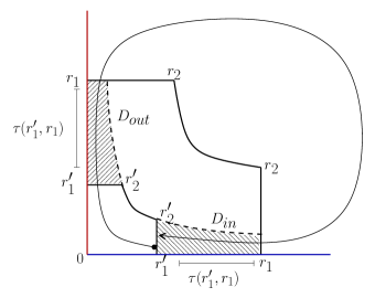
Figure 19: The returning time to the annulus at position $r_{1}\times[0,r_{2}]\times\mathbb{R}/\mathbb{Z}$ increases when $r_{2}/r_{1}\to 0$.

Proof of lemma 5.11.

We will use the constants $\varepsilon$, $C$, and $D$ defined in the proof of lemma 5.10. Let $v_{1},v_{2}\in C^{cu}(p;\delta_{0}^{u},\delta_{1}^{u})$. By (50) the action of each transformation $\Psi_{t}$ has the effect of contract the difference of slopes between $v_{1}$ and $v_{2}$ by a ratio exponential in $t$. More precisely,

$$\left|\Delta_{u}(\Psi_{t}(v_{2}))-\Delta_{u}(\Psi_{t}(v_{1}))\right|=\lambda^{2t}\left|\Delta_{u}(v_{2})-\Delta_{u}(v_{1})\right|,\ \text{for all}\ t\geq 0.$$ (57)

For a point $q\in A_{in}^{1}$ consider two vectors $v_{i}=b_{i}\bar{e}_{s}+c_{i}\bar{e}_{u}$ in $\bar{H}^{su}(q)$ and let $(r_{1},r,s)$ be the coordinates of $q$. First, we claim that if $|\Delta_{u}(v_{2})-\Delta_{u}(v_{1})|<\varepsilon$ then

$$\left|\Delta_{u}(\Phi_{q}(v_{2}))-\Delta_{u}(\Phi_{q}(v_{1}))\right|\leq\left|\Delta_{u}(v_{2})-\Delta_{u}(v_{1})\right|.$$ (58)

To see this, consider a vector $v=b\bar{e}_{s}+c\bar{e}_{u}$ and denote its $u$-slope by $\delta=b/c$. From the expression of $\Phi_{q}$ is $su$-coordinates in (51) we have that

$$\Delta_{u}(v)=\frac{(b/c)(K(r,r_{2})+1)+K(r,r_{2})\frac{r_{1}}{r}}{-(b/c)K(r,r_{2})\frac{r}{r_{1}}+(1-K(r,r_{2}))}.$$

Denote by $\delta\mapsto g(\delta)$ the family of rational functions obtained by setting $\delta=b/c$. Then

$$g^{\prime}(\delta)=\frac{1}{\left(-\delta K(r,r_{2})\frac{r}{r_{1}}+(1-K(r,r_{2}))\right)^{2}}<1,\ \text{for all}\ -r_{1}/r\leq\delta\leq 0.$$

We conclude the claim (58), since $\varepsilon<r_{1}/r$ for every $r$ where $\Phi_{q}\neq id$. Second, by (55) we can see that $g^{\prime}$ has no poles for for slopes $-3r_{1}/r_{2}\leq\delta\leq 0$, so there is a constant $K_{0}>0$ such that

$$\left|\Delta_{u}(\Phi_{q}(v_{2}))-\Delta_{u}(\Phi_{q}(v_{1}))\right|\leq K_{0}\left|\Delta_{u}(v_{2})-\Delta_{u}(v_{1})\right|,\ \forall\ v_{1},v_{2}\in C^{cu}(q;\delta^{u}_{0},\delta^{u}_{1}).$$ (59)

Given $p\in N$ and $t\geq 0$, by lemma 5.6 there exist $t_{1},\dots,t_{l+1}>0$ and $p_{1},\dots,p_{l+1}\in A_{in}^{1}$, such that $t=t_{1}+\cdots t_{l+1}$, $t_{n}\geq T_{1}(r_{1},r_{2})$ for $n=2,\dots,l$ (cf. proof of 5.10) and the action of $D\psi_{t}(p)$ on $TN$ decomposes as a product of transformations $\Psi_{t_{n}}$ and $\Phi_{p_{n}}$. Fix two vectors $v_{1},v_{2}\in C^{cu}(p,\delta^{u}_{0},\delta^{u}_{1})$. Using (57) and (59) we see that

$$\left|\Phi_{p_{1}}\circ\Psi_{t_{1}}(v_{2})-\Phi_{p_{1}}\circ\Psi_{t_{1}}(v_{1})\right|\leq\lambda^{t_{1}}K_{0}\left|\Delta_{u}(v_{2})-\Delta_{u}(v_{1})\right|.$$

For each $i=1,2$ define $v_{i}^{1}=\Phi_{p_{1}}\circ\Psi_{t_{1}}(v_{i})$ and for $n\geq 2$ define $v_{i}^{n}=\Phi_{t_{n}}\circ\Psi_{p_{n}}(v_{i}^{n-1})$. Since $v_{1}^{1},v_{2}^{1}\in C^{cu}(\varphi(p_{1};-Cr_{1}/r_{2},Dr_{2}/r_{1}))$ and since $t_{n}\geq T_{1}$ for $n\geq 2$, we have that $v_{i}^{n}\in C^{cu}(-\varepsilon,\varepsilon),\ \forall\ n\geq 2$ (cf. proof of lemma 5.10). In particular, using (58) we have

$$\left|\Delta_{u}(v_{2}^{n})-\Delta_{u}(v_{1}^{n})\right|\leq\lambda^{2t_{n}}\left|\Delta_{u}(v_{2}^{n})-\Delta_{u}(v_{1}^{n})\right|,\ \forall\ n\geq 2,$$

from where we deduce

$$\left|\Delta_{u}(D\psi_{t}(p)\cdot v_{2})-\Delta_{u}(D\psi_{t}(p)\cdot v_{1})\right|\leq\lambda^{2\left(t_{1}+\cdots t_{l+1}\right)}\cdot K_{0}\cdot\left|\Delta_{u}(v_{2})-\Delta_{u}(v_{1})\right|.$$

Finally, since $|\Delta_{u}(v_{2})-\Delta_{u}(v_{1})|\leq\delta^{u}_{1}-\delta^{u}_{0}$, we can bound the right side of this inequality by $\lambda^{2t}L_{0}$, where $L_{0}=K_{0}(\delta^{u}_{1}-\delta^{u}_{0})>0$. This completes the $cu$-case.

The analogous reasoning applies for $C^{cs}(p;\delta_{0}^{s},\delta_{1}^{s})$ and the backward action of the flow. ∎

Proof of lemma 5.12.

Let $p\in N$, $v\in T_{p}N$ and $t\geq 0$. Using the basis defined in (45), write $v=aY(p)+be_{s}(p)+ce_{u}(p)$ and define $\|v\|_{su}=\sqrt{b^{2}+c^{2}}$. We remark that $\|D\psi_{t}(v)\|=\sqrt{a^{2}+\|D\psi_{t}(v)\|_{su}^{2}}$ for $t\geq 0,$ so it suffices to show that the statement of the lemma is satisfied using $\|\cdot\|_{su}$. Let’s call $\delta=\Delta_{u}(v)=b/c$ and assume that $-\infty<\delta<\infty$.

From the one hand, let $q\in A_{in}^{1}$ and $v\in T_{q}N$. Since $p\mapsto\Phi_{q}$ has compact support, by taking $R_{0}=\min\left\{\left(\|\Phi_{q}^{-1}\|_{\infty}\right)^{-1}:a\in A_{in}^{1}\right\}>0$ we have

$$\|\Phi_{q}(v)\|_{su}>R_{0}\|v\|_{su},\ \text{for all}\ v\in T_{q}N.$$ (60)

Moreover, consider $0<\varepsilon<3r_{1}/2r_{2}$ defined in the proof of lemma 5.10. From the expression (52) it follows that

$$\|\Phi_{q}(v)\|_{su}>\|v\|_{su},\ \text{for all}\ v\in C^{cu}(q;-\varepsilon,\varepsilon).$$ (61)

From the other hand, since the transformations $\Psi_{t}$ on the $su$-plane correspond to the hyperbolic matrices (50), it follows that for every $v\in TN$ there exists $0<Q(\delta)=(\delta^{2}+1)^{-1}\leq 1$ such that

$$\|\Psi_{t}(v)\|_{su}\geq Q(\delta)\lambda^{-t}\|v\|_{su},\ \forall\ t\geq 0.$$ (62)

To see an expansion on the $su$-norm by an application of $\Psi_{t}$ on $v$, we need to wait some time depending on the slope of $v$. It can be seen that, if $|\delta|\leq 1/2$ then $|\Psi_{t}(v)|_{su}>|v|_{su}$, $\forall\ t\geq 0$, and if $|\delta|>1/2$ then $|\Psi_{t}(v)|_{su}>|v|_{su}$ if and only if $\Delta_{u}(\Psi_{t}(v))>1/|\delta|$.

Consider $T_{0}=T_{0}(r_{1},r_{2})>0$ such that

$$-\frac{1}{C}\frac{r_{2}}{r_{1}}<-\lambda^{2T_{0}(r_{1},r_{2})}C\frac{r_{1}}{r_{2}}<0<\lambda^{2T_{0}(r_{1},r_{2})}D\frac{r_{2}}{r_{1}}<\frac{1}{D}\frac{r_{1}}{r_{2}},$$

where $C,D>0$ are the constants defined along the proof of lemma 5.10. Defined in this way, $T_{0}$ is the minimal time needed to see an expansion of $\|\Psi_{t}(v)\|_{su}$ for vectors $v$ in the cone $C^{cu}(p;-Cr_{1}/r_{2},$ $Dr_{2}/r_{1})$. For such a choice of $T_{0}$ we have that

$$\|\Psi_{T_{0}}(v)\|_{su}\geq Q_{0}\lambda^{-T_{0}}\|v\|_{su}>\|v\|_{su},\ \text{for all}\ -Cr_{1}/r_{2}<\Delta_{u}(v)<Dr_{2}/r_{1},$$

where $Q_{0}=\min\left\{Q(-Cr_{1}/r_{2}),Q(Dr_{2}/r_{1})\right\}$. We define $\mu=Q_{0}^{1/T_{0}}\lambda^{-1}$, which satisfies $1<\mu<1/\lambda$.

Since $T_{0}(r_{1},r_{2})$ depends just on $r_{1}/r_{2}$, we can shrink both $r_{1}$ and $r_{2}$, keeping constant its ratio, in such a way that the minimal returning time $T_{1}=T_{1}(r_{1},r_{2})$ of points in the support of the surgery to itself is greater that $T_{0}(r_{1},r_{2})$, cf. proof of lemma 5.10.

Assuming this condition, let $p\in N$, $t\geq 0$, $v\in C^{cu}(p;\delta_{0}^{u},\delta_{1}^{u})$ and consider the decomposition $D\psi_{t}(p)\cdot v=\Psi_{t_{l+1}}\cdot\Phi_{p_{l}}\cdots\Phi_{p_{1}}\cdot\Psi_{t_{1}}(v)$, where $l\geq 0$, $t_{k}\geq T_{1}\geq T_{0}$ for $k=2,\dots,l$ and $p_{k}\in A_{in}^{1}$. Define $v^{1}=\Phi_{p_{1}}\circ\Psi_{t_{1}}(v)$ and for $k=2,\dots,l$ define $v^{k}=\Psi_{t_{k}}\circ\Phi_{p_{k}}(v^{k-1})$. It follows that

1. By (62) and (60) then

   $$\|v^{1}\|_{su}\geq\left(\|\Phi_{p_{1}}^{-1}\|_{\infty}\right)^{-1}\|\Psi_{t_{1}}(v)\|_{su}\geq R_{0}Q_{0}\cdot\lambda^{-t_{1}}\|v\|_{su}.$$

2. Since $v^{1}\in C^{cu}(p_{1};-Cr_{1}/r_{2},Dr_{2}/r_{1})$ and $t_{k}\geq T_{0}$ for $k=2,\dots,l$, then $v^{k}\in C^{cu}(p_{k};-\varepsilon;\varepsilon)$ (cf. proof of lemma 5.10). By (61) and (62) then

   $$\|v^{k}\|_{su}\geq Q_{0}\lambda^{-t_{k}}\|v^{k-1}\|_{su},\ \text{for}\ k=2,\dots,l.$$

Therefore, putting together (i) and (ii) above in the decomposition $D\psi_{t}=\Psi_{t_{l+1}}\cdot\Phi_{p_{l}}\cdots\Phi_{p_{1}}\cdot\Psi_{t_{1}}$, and using the fact that $0\leq l\leq t/T_{1}$, we obtain

$$\|D\psi_{t}(p)\cdot v\|_{su}\geq R_{0}Q_{0}^{l+1}\lambda^{-(t_{1}+\cdots+t_{k+1})}\|v\|_{su}$$

$$\geq (R_{0}Q_{0})Q_{0}^{t/T_{1}}\lambda^{-t}\|v\|_{su}\geq(cte)\cdot\mu^{t}\|v\|_{su}.$$

∎

5.4.2 Existence of the strong-stable and strong-unstable invariant distributions.

We prove now that, for small values of $0<r_{2}<r_{1}<1$, the flow $(\psi_{t},N)$ constructed proposition 5.3 preserves a hyperbolic splitting of the form $TN=F^{s}\oplus H^{c}\oplus F^{u}$, where $H^{c}=\textsl{span}\{Y\}$ as before.

We will show that each plane $F^{cu}$ and $F^{cs}$ has a decomposition $F^{cu}=H^{c}\oplus F^{u}$ and $F^{cs}=F^{s}\oplus H^{c}$, respectively, where $F^{s}$ and $F^{u}$ are $D\psi_{t}$-invariant one dimensional bundles, contacting and expanding. For doing this, inside each plane $F^{cu}$ and $F^{cs}$ we will chose a cone distribution that satisfy the cone field criterion. Since the method is analogous to the previous one, we do not complete all the proof, but we sketch the general arguments. We will make the argument just for $cu$-case, being analogous the other case.

Proposition 5.13.

There exist two continuous line distributions $F^{s}$ and $F^{u}$ in the tangent bundle $TN$ satisfying that:

1. $D\psi_{t}(p)\left(F^{u}(p)\right)=F^{u}(\psi_{t}(p))$ and $D\psi_{t}(p)\left(F^{s}(p)\right)=F^{s}(\psi_{t}(p))$, for every $p\in N$ and $t\in\mathbb{R}$;

2. $F^{cs}(p)=F^{s}(p)\oplus H^{c}(p)$ and $F^{cu}(p)=H^{c}(p)\oplus F^{u}(p)$, $\forall$ $p\in N$, where $H^{c}(p)=\textsl{span}\{Y(p)\}$;

3. There exists constants $L>0$ and $\mu>1$ such that

   $$\|D\psi_{t}(p)\cdot v\ \|\geq L\mu^{t}\|v\|,\ \forall\ p\in N,\ v\in F^{u}(p),\ t\geq 0,$$

   $$\|D\psi_{-t}(p)\cdot v\|\geq L\mu^{t}\|v\|,\ \forall\ p\in N,\ v\in F^{s}(p),\ t\geq 0.$$

We will still make use of the decomposition $TN=H^{s}\oplus H^{c}\oplus H^{u}$ defined in (45). It is convenient to recall that, if we see $N$ as the union of $M_{0}$ and $M_{1}$, by definition this decomposition coincides with the splitting $E^{s}_{i}(p)\oplus E^{c}(p)_{i}\oplus E^{u}_{i}(p)$ associated to the vector field $X_{i}$ when $p\in M_{i}$, $i=1,2$. To prove this proposition we define:

Inclination of the plane $F^{cu}$.

Given a point $p\in M_{i}$, since each plane $F^{cu}(p)$ is contained in the cone $C^{cu}(p;\delta_{0}^{u},\delta_{1}^{u})$, there exists a slope value $\delta_{0}^{u}\leq\alpha_{i}(p)\leq\delta_{1}^{u}$ verifying that

$$F^{cu}(p)=\left\{v\in T_{p}M_{i}:v=aX_{i}(p)+\alpha_{i}(p)ce_{s}^{i}(p)+ce_{u}^{i}(p):a,c\in\mathbb{R}\right\}.$$

Since the plane distribution is continuous as a function of $p\in N$, then each $\alpha_{i}:M_{i}\to\mathbb{R}$, $i=1,2$ is continuous. Moreover, at each $p\in M_{0}\cap M_{1}$ the chart $\Phi_{p}$ defined in (49) must verify

$$\Phi_{p}: \left\{aX_{0}(p)+\alpha_{0}(p)ce_{s}^{0}(p)+ce_{u}^{0}(p):a,c\in\mathbb{R}\right\}\mapsto$$

$$\left\{aX_{1}(\varphi(p))+\alpha_{1}(\varphi(p))ce_{s}^{1}(\varphi(p))+ce_{u}^{1}(\varphi(p)):a,c\in\mathbb{R}\right\}.$$

Observe that this imposes a relation between the values $\alpha_{0}(p)$ and $\alpha_{1}(\varphi(p))$. Since the change of coordinates $\Phi_{p}:T_{p}M_{0}\to T_{\varphi(p)}M_{1}$ is the identity when $p$ is not in $A_{in}^{1}$, we obtain a slope function $\alpha:N\to[\delta_{0}^{u},\delta_{1}^{u}]$ that is continuous in the complement of this annulus.

Framing on $F^{cu}$

For every $p\in N$ the subspace $H^{s}(p)$ is transverse to both $H^{c}(p)\oplus H^{u}(p)$ and $F^{cu}(p)$. Thus, there exists an isomorphism $P^{s}(p):F^{cu}(p)\to H^{c}(p)\oplus H^{u}(p)$ obtained by projecting $F^{cu}(p)$ onto $H^{c}(p)\oplus H^{u}(p)$ in the direction of $H^{s}(p)$. This allows to define a decomposition

$$F^{cu}(p)=H^{c}(p)\oplus\tilde{H}^{u}(p),$$ (63)

where $\tilde{H}^{u}(p)$ is the pull-back bundle of $H^{u}(p)$ by $P^{s}(p)$. Recall that the line bundle $H^{c}$ is collinear with the vector field $Y$, thus continuous. As before, it can be seen that the bundle $\tilde{H}^{u}$ does not varies continuously as a functions of $p$, the discontinuity set being contained in the support of the surgery inside $A_{in}^{1}$.

Action on the $F^{cu}$-bundle.

Let $p\in N$ and $t\geq 0$. Since the distribution $F^{cu}$ is invariant under the action of $D\psi_{t}$, using lemma 5.6 we can write

$$\left(D\psi_{t}|_{F^{cu}}\right)(p)=\left(\Psi_{t_{l+1}}|_{F^{cu}}\right)\cdot\left(\Phi_{p_{l}}|_{F^{cu}}\right)\cdot\left(\Psi_{t_{l}}|_{F^{cu}}\right)\cdots\left(\Phi_{p_{1}}|_{F^{cu}}\right)\cdot\left(\Psi_{t_{1}}|_{F^{cu}}\right)(p).$$ (64)

for some $p_{1},\dots,p_{l}\in A_{in}^{1}$ and $t_{k}>0$, uniformly bounded from below for $k=2,\dots,l$. We need to describe each family of transformations $\Psi_{t}$ and $\Phi_{q}$ acting on $F^{cu}$.

For every $p\in N$ consider a basis $\{e_{c}(p),\tilde{e}_{u}(p)\}$, where $e_{c}(p)=Y(p)$ and $\tilde{e}_{u}(p)=\alpha(p)e_{s}(p)+e_{u}(p)$ is a vector in $\tilde{H}^{u}(p)$. It follows that:

1. If the orbit segment segment $[p,\psi_{t}(p)]$ does not intersect the annulus $A_{in}^{1}$, then the inclination of the planes $F^{cu}$ along this segment satisfies the relation $\alpha(\psi_{s}(p))=\lambda^{2s}\alpha(p)$, $0\leq s\leq t$. This can be deduced from the formula (50) for the action of $\Psi_{t}$ on the $su$-bundle and the invariance of the planes $F^{cu}$. As a consequence we have:

   $$\left(\Psi_{t}|_{F^{cu}}\right)_{c\tilde{u}}=\begin{pmatrix}1&0\\ 0&\lambda^{-t}\end{pmatrix}.$$ (65)

2. If $q\in A_{in}^{1}$ is a point with normal coordinates $q=(r_{1},r,s)$, then using (48) we can see that

   $$\left(\Phi_{q}|_{F^{cu}}\right)_{c\tilde{u}}=\begin{pmatrix}1&A(r,r_{1},r_{2})\\ 0&B(r,r_{1},r_{2})\end{pmatrix},$$ (66)

   $$\text{where}\ \ \left\{\begin{array}[]{lll}A(r,r_{1},r_{2})=-\frac{1}{r_{2}\log(\lambda)}K(r_{1},r_{2})\left(\alpha(q)\frac{r}{r_{1}}+1\right)\\ B(r,r_{1},r_{2})=-K(r_{1},r_{2})\left(\alpha(q)\frac{r}{r_{1}}+1\right)+1.\end{array}\right.$$ (69)

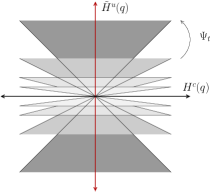
(a) $\Psi_{t}$

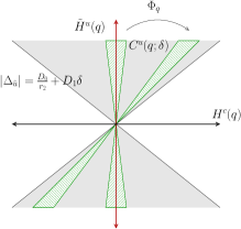
(b) $\Phi_{q}$

Figure 20: Action on the $F^{cu}$ plane distribution.

Choice of cone distributions.

We will define the $\tilde{u}$-slope of a vector $v=ae_{c}(p)+c\tilde{e}_{u}(p)$ in $F^{cu}(p)$ by $\Delta_{\tilde{u}}(v)=\frac{a}{c}.$ Given a fixed real number $\delta>0$, for every $p\in N$ define the cone $C^{u}(p;\delta)=\left\{v\in F^{cu}(p)\right.$ $\left.:\ -\delta\leq\Delta_{\tilde{u}}(v)\leq\delta\right\}.$ For choosing an adequate cone distribution in $F^{cu}$ that satisfies the cone field criterion, we will make use of the following:

Claim.

There exist positive constants $D_{0}=D_{0}(r_{2}/r_{1})$ and $D_{1}=D_{1}(r_{2}/r_{1})$ such that, for every $\delta>0$,

$$\left|\Delta_{\tilde{u}}\left(\Phi_{q}(v)\right)\right|\leq\frac{D_{0}}{r_{2}}+D_{1}\delta,\ \text{for every}\ q\in A_{in}^{1}\ \text{and}\ v\in C^{u}(p;\delta).$$ (70)

Assuming this claim, define

$$\delta^{u}\coloneqq(D_{0}/r_{2})+1.$$

Proposition 5.13 reduces to prove the following three statements:

Lemma 5.14.

If $0<r_{2}<r_{1}<1$ are sufficiently small, then there exists $T>0$ such that: For every $p\in N$ then

$$D\psi_{t}\left(C^{u}(p;\delta^{u})\right)\subset C^{u}\left(\psi_{t}(p);\delta^{u}\right),\ \text{for every}\ t\geq T.$$

Lemma 5.15.

For the parameters $0<r_{2}<r_{1}<1$ given in the previous lemma, it is satisfied the following: There exists a constant $\tilde{L}_{0}>0$ such that, for every $p\in N$ and every $t\geq 0$ then

$$\left|\ \Delta_{\tilde{u}}(D\psi_{t}(p)\cdot v_{2})-\Delta_{\tilde{u}}(D\psi_{t}(p)\cdot v_{1})\ \right|\leq\lambda^{t}\tilde{L}_{0},\ \forall\ v_{1},v_{2}\in C^{u}(p;\delta^{u}).$$

Lemma 5.16.

By shrinking the parameters $0<r_{2}<r_{1}<1$ of the previous lemmas if necessary, it is satisfied that: There exist constants $\tilde{L}>0$ and $\tilde{\mu}>1$ such that, for every $p\in N$ and every $t\geq 0$ then

$$\left\|D\psi_{t}(p)\cdot v\ \right\|\geq\tilde{L}\tilde{\mu}^{t}\|v\|,\ \forall\ v\in C^{u}(p;\delta^{u}).$$

The proof of proposition 5.13 and the subsequent lemmas is similar to that of proposition 5.9 for the $cu$- case, so we just sketch the main arguments.

Proof of prop. 5.13 and lemmas 5.14, 5.15, 5.16.

To prove proposition 5.13, choose $0<r_{2}<r_{1}<1$ satisfying the conditions of proposition 5.9 and lemmas 5.14, 5.15, 5.16. Then we can pointwise define a cone distribution $p\mapsto F^{u}(p)\subset F^{cu}(p)$ by the expression

$$F^{u}(p)=\bigcap_{k\geq 0}D\psi_{kT}(p)\left(C^{u}(\psi_{-kT}(p));\delta^{u}\right).$$

By 5.14 we have that this is a well-defined cone distribution, and by 5.15 we have that the cones are degenerated, so it is in fact a line distribution. Then, by 5.16 we obtain that $F^{u}(p)$ is an expansive bundle, which in turn implies that $F^{cu}(p)=F^{u}(p)\oplus H^{c}(p)$ is a dominated splitting, unique, invariant and continuous.

Before the lemmas we prove the claim above in (70): Using the formula (66) for the matrix $\Phi_{q}$ in $cu$-coordinates, for every $v\in F^{cu}(q)$ we have that

$$\Delta_{\tilde{u}}\left(\Phi_{q}(v)\right)= \frac{A(r,r_{1},r_{2})}{B(r,r_{1},r_{2})}+\frac{\Delta_{\tilde{u}}(v)}{B(r,r_{1},r_{2})}$$

$$= \frac{1}{r_{2}\log(\lambda)}\left(\frac{-K(r_{1},r_{2})(\alpha(q)r/r_{1}+1)}{-K(r_{1},r_{2})(\alpha(q)r/r_{1}+1)+1}\right)$$

$$+\Delta_{\tilde{u}}(v)\left(\frac{1}{-K(r_{1},r_{2})(\alpha(q)r/r_{1}+1)+1}\right).$$

Observe that the function $B(r,r_{1},r_{2})$ has no zeros (since the matrix $(\Phi_{q})_{cu}$ in (66) is always an isomorphism) and equals one when $r\notin[r_{2}/3,2r_{2}/3]$, so there exists $K_{0}>0$ such that $B(r,r_{1},r_{2})\geq K_{0}$ for $0\leq r\leq r_{2}$. Using that $K(r_{1},r_{2})$ equals $r/r_{2}$ up to multiplication by a bounded function and $K(r,r_{2})=0$ if $r\notin[r_{2}/3,2r_{2}/3]$ we can see that $K_{0}$ depends just on the ratio $r_{2}/r_{1}$. Therefore, there are two constants $D_{0}(r_{2}/r_{1})$ and $D_{1}(r_{2}/r_{1})$ such that $|\Delta_{\tilde{u}}(\Phi_{q}\cdot v)|\leq(D_{0}/r_{2})+D_{1}\delta$, for every $|\Delta_{\tilde{u}}(v)|\leq\delta.$ This proves the claim.

Recall that $\delta^{u}=(D_{0}/r_{2})+1$ and define $\kappa=(D_{0}/r_{2})+D_{1}\delta^{u}+1$. Following the claim above there exists $\varepsilon=\varepsilon(r_{2}/r_{1})>0$ such that

$$\Phi_{q}\left(C^{u}(q;\varepsilon)\right)\subset C^{u}(\varphi(q);\delta^{u}),\ \forall\ q\in A_{in}^{1},$$ (71)

$$\Phi_{q}\left(C^{u}(q;\delta^{u})\right)\subset C^{u}(\varphi(q);\kappa),\ \forall\ q\in A_{in}^{1}.$$ (72)

From the other hand, observe that each transformation $\Psi_{t}$ acting on $F^{cu}$ satisfies

$$\Psi_{t}\left(C^{u}(p;\delta)\right)=C^{u}(\psi_{t}(p);\lambda^{t}\delta),$$ (73)

for any $\delta$, as follows simply by (65) above. Let $T_{1}(r_{1},r_{2})$ be the minimal returning time of points contained in the annulus $\{q=(r,r_{1},r_{2})\in A_{in}^{1}:r_{2}/3\leq r\leq 2r_{2}/3\}$, as defined in the course of the proof of lemma 5.10. We claim that:

Claim.

If we shrink sufficiently the parameters $0<r_{2}<r_{1}<1$ keeping constant its ratio $r_{2}/r_{1}$, then it follows that $0<\lambda^{T_{1}(r_{1},r_{2})}\kappa<\varepsilon.$

Assuming this claim, we can proceed to prove the three lemmas stated above. Start with some model $(\psi_{t},N)$ corresponding to two fixed parameters $0<r_{2}<r_{1}<1$. If we shrink the parameters keeping constant the ratio in order to satisfy the claim, we encounter that $t_{k}\geq T_{1}(r_{1},r_{2})$ for $k=2,\dots,l$ in the decomposition given in (64). Then:

1. Using (71)-(72)-(73) we have that each map $\left(\Psi_{t_{k}}|_{F^{cu}}\right)\circ\left(\Phi_{p_{k-1}}|_{F^{cu}}\right)$ sends the cone $C^{u}(p_{k};\delta^{u})$ inside $C^{u}(p_{k+1};\delta^{u})$, for $k=2,\dots,l$. Thus, if we choose $T\geq 2T_{1}(r_{1},r_{2})$, we can conclude in the same way as in 5.10.

2. For the second lemma, observe that the transformations $\Phi_{p_{k}}$ satisfy that, for every pair of vectors $v_{1}$, $v_{2}$ in $F^{cu}$,

   $$\left|\Delta_{\tilde{u}}\left(\Phi_{p_{k-1}}(v_{2})\right)-\Delta_{\tilde{u}}\left(\Phi_{p_{k-1}}(v_{1})\right)\right|\leq D_{1}\left|\Delta_{\tilde{u}}(v_{2})-\Delta_{\tilde{u}}(v_{1})\right|.$$

   Since the transformations $\Psi_{t_{k}}$ contract slopes at an exponential rate, if we adjust $r_{1},r_{2}$ in order to have a big enough $T_{1}(r_{1},r_{2})$ such that $0<\lambda^{T_{1}}D_{1}<1$, then each map $\left(\Psi_{t_{k}}|_{F^{cu}}\right)\circ\left(\Phi_{p_{k-1}}|_{F^{cu}}\right)$ contracts $|\Delta_{\tilde{u}}(v_{2})-\Delta_{\tilde{u}}(v_{1})|$ by a factor strictly lower that one. By writing $D\psi_{t}$ as an alternated composition of these transformations, we obtain the conclusion of the lemma.

3. For the third lemma observe that, for every vector $v\in F^{cu}$ in the cone $-\delta^{u}\leq\Delta_{\tilde{u}}(v)\leq\delta^{u}$, from the one side using (65) we have that $\|\Psi_{t_{k}}(v)\|_{cu}\geq(cte)\cdot\lambda^{-t_{k}}\|v\|_{cu}$. From the other side, the minimum

   $$d=d(r_{2}/r_{1})=\min\left\{\left\|\Phi_{q}(v)\right\|_{cu}:\|v\|_{cu}=1,\ q\in A_{in}^{1}\right\}$$

   depends only on the quantity $r_{2}/r_{1}$ and is positive, as can be seen from the of the quantities participating in formula (66). We obtain $\|\Phi_{q}(v)\|_{cu}\geq d\|v\|_{cu}$, independently of $q$. Thus, shrinking $r_{1}$ and $r_{2}$ in the appropriate way if necessary, we have that each transformation $\left(\Psi_{t_{k}}|_{F^{cu}}\right)\circ\left(\Phi_{p_{k-1}}|_{F^{cu}}\right)$ expands norms in the $cu$-plane by a factor grater that $1<(cte)\cdot\lambda^{-t_{k}}d$. By writing $D\psi_{t}$ as an alternated composition of these transformations, we obtain the conclusion of the lemma.

Finally, to prove the claim, start with two fixed values $0<r_{2}<r_{1}<1$ and let $\beta=r_{2}/r_{1}$. Let $0<r_{2}^{\prime}<r_{1}^{\prime}<1$ satisfying that $0<r_{2}^{\prime}<r_{2}$, $0<r_{1}^{\prime}<r_{1}$ and $r_{2}^{\prime}/r_{1}^{\prime}=\beta$. As in the proof of lemma 5.10, the returning time $T_{1}(r_{1},r_{2})$ satisfies that

$$T_{1}(r_{1},r_{2})\geq\tau(r_{1}^{\prime},r_{1})=\frac{1}{\log(\lambda)}\log\left(\frac{(r_{1}^{\prime})^{2}}{r_{1}^{2}}\right).$$

Thus,

$$\lambda^{T_{1}(r_{1},r_{2})}\left(\frac{D_{0}}{r_{2}^{\prime}}+D_{1}\delta\right)\leq\lambda^{\tau(r_{1}^{\prime},r_{1})}\left(\frac{D_{0}}{r_{2}^{\prime}}+D_{1}\delta\right)\leq\frac{(r_{1}^{\prime})^{2}}{r_{1}^{2}}\left(\frac{D_{0}}{\beta r_{1}^{\prime}}+D_{1}\delta\right),$$

which can be made smaller than $\delta/2$ if $r_{1}^{\prime}$ is small enough. We can conclude that, for small values of $r_{1}^{\prime}$, the couple $r_{1}^{\prime}$, $r_{2}^{\prime}$ satisfies the claim. ∎

5.5 Equivalence with the original flow.

The general setting at the beginning of section 5 is a transitive topological Anosov flow $(\phi_{t},M)$ equipped with a Birkhoff section $\iota:(\Sigma,\partial\Sigma)\to(M,\Gamma)$ which, for simplicity, we have assumed to have only one orbit $\gamma\in\Gamma$. In subsection 5.3 we have constructed a smooth flow $(\psi_{t},N)$ depending on the combinatorial parameters $p(\gamma,\Sigma)$, $n(\gamma,\Sigma)$, $m(\gamma,\Sigma)$ of the Birkhoff section and on two real parameters $0<r_{2}<r_{1}<1$. Then, in subsection 5.4 we have showed that if $r_{1},r_{2}$ are chosen small enough, the flow $(\psi_{t},N)$ is Anosov.

We show here that if $0<r_{2}<r_{1}<1$ are sufficiently small such that $(\psi_{t},N)$ is Anosov, then $(\psi_{t},N)$ is orbitally equivalent to the original flow $(\phi_{t},M)$. We do it by checking the criterion provided in theorem A.

Proposition 5.17.

The flow $(\psi_{t},N)$ constructed in proposition 5.3 is orbitally equivalent to the original flow $(\phi_{t},M)$, provided $0<r_{2}<r_{1}<1$ are sufficiently small.

To check the criterion in theorem B, the flow $(\phi_{t},M)$ is already endowed with a Birkhoff section and we have to show that $(\psi_{t},N)$ admits a (homeomorphic) Birkhoff section, that carries the same first return action on fundamental group and the same combinatorial data on the boundary.

It will be convenient to recall the general construction of the manifold $N=M_{0}\sqcup_{\varphi}M_{1}$. Using the charts $\{\Pi_{i}:i=1,\dots,4\}$ from proposition 4.4 we have defined a family of compact tubular neighbourhoods $R(r_{1},r_{2})\subset M$ of the orbit $\gamma$. Then $N$ is constructed by removing from $M$ the interior of such a tubular neighbourhood, obtaining a manifold $M_{0}$ with boundary $\partial M_{0}=\partial R(r_{1},r_{2})$, and then glueing along the boundary the solid torus $M_{1}=\mathbb{V}(r_{1},r_{2})$. The glueing map $\varphi:\partial M_{0}\to\partial M_{1}$ given in definition (38)-(39) has support contained in the annulus $A_{in}^{1}$ inside the first quadrant of $R(r_{1},r_{2})$, or in $A_{in}^{4}$ in the fourth quadrant, depending on the signature of $m=m(\gamma,\Sigma)$.

Lemma 5.18.

There exists an immersion $\zeta:\Sigma\to N$ verifying that:

1. $\zeta:(\Sigma,\partial\Sigma)\to(N,\gamma_{0})$ is a Birkhoff section that sends the boundary components of $\Sigma$ onto the periodic orbit $\gamma_{0}$ contained in $M_{1}$.

2. If we call $\Sigma^{\prime}=\zeta(\Sigma)$, then $n(\gamma_{0},\Sigma^{\prime})=n(\gamma,\Sigma)$, $m(\gamma_{0},\Sigma^{\prime})=m(\gamma,\Sigma)$ and $p(\gamma_{0},\Sigma^{\prime})=p(\gamma,\Sigma)$.

3. $\zeta(\Sigma)\cap M_{0}\equiv\iota(\Sigma)\cap M_{0}$.

Proof.

We will make the proof for the case $m=m(\gamma,\Sigma)<0$, being analogue the other case. For simplicity, we will assume as well that $p(\gamma,\Sigma)=1$.

Since $N=M_{0}\sqcup_{\varphi}M_{1}$ and $M=M_{0}\sqcup_{id}R(r_{1},r_{2})$, we will consider the component $M_{0}$ as included in both $N$ and $M$. Define $\Sigma_{0}=\iota(\Sigma)\cap M_{0}$, which is the part of the original Birkhoff section that lies outside the neighbourhood $R(r_{1},r_{2})$. To prove the lemma, we will show that $\Sigma_{0}$ can be extended inside the manifold $M_{1}$, adding an helicoidal-like surface $S$ that connects $\partial\Sigma_{0}$ with $\gamma_{0}$, in such a way to obtain the desired Birkhoff section.

Let $\alpha=\partial\Sigma_{0}=\Sigma_{0}\pitchfork\partial M_{0}$. By construction of $R(r_{1},r_{2})$, this curve is a piecewise smooth, simple, closed curve in $\partial R(r_{1},r_{2})$. The partition into quadrants of $R(r_{1},r_{2})$ originates a partition of $\alpha$ into segments

$$\left\{\alpha_{in}^{i+4j},\alpha_{tg}^{i+4j},\alpha_{out}^{i+4j};\ i=1,\dots,4,\ k=0,\dots,4n-1\right\}$$

of constant $\mathbb{R}/\mathbb{Z}$-coordinate, as in the left part of figure (16). We choose the supra-index $i+4j$ in such a way that each $\alpha^{i+4j}_{*}$ is contained in the quadrant $R_{i}(r_{1},r_{2})$, $i=1,\dots,4$, and we use the sub-index $in,\ tg,\ out$ to indicate if the segment belongs to the region of $\partial R(r_{1},r_{2})$ where the flow enters, is tangent or escapes the neighbourhood $R(r_{1},r_{2})$, respectively.

Let $\beta=\varphi(\alpha)$, which is a piecewise smooth, simple, closed curve contained in $\partial\mathbb{V}(r_{1},r_{2})$. In an analogous fashion, the curve $\beta$ can be decomposed in a concatenation of compact segments

$$\left\{\beta_{in}^{i+4j},\beta_{tg}^{i+4j},\beta_{out}^{i+4j};\ i=1,\dots,4,\ k=0,\dots,4n-1\right\},$$

as in figures (16) or (21). Since $\varphi$ restricts to a monotonous twist on the annulus $A_{in}^{1}$ and to the identity on the complement, we find that each segment $\beta_{in}^{1+4j}$ (in the first quadrant) admits a parametrization with monotonous $\mathbb{R}/\mathbb{Z}$-coordinate, while every other segment $\beta_{*}^{i+4j}=\varphi(\alpha_{*}^{i+4j})=\alpha_{*}^{i+4j}$ has constant $\mathbb{R}/\mathbb{Z}$-coordinate.

Claim.

There exists an immersion $S\hookrightarrow\mathbb{V}(r_{1},r_{2})$, where $S$ is a compact annulus, satisfying that:

1. One boundary component of $S$ coincides with $\beta=S\cap\partial\mathbb{V}(r_{1},r_{2})$,

2. The immersion is actually a local Birkhoff section at $\gamma_{0}$ for the flow $\psi_{t}$, with $n(\gamma_{0},S)=n(\gamma,\Sigma)$ and $m(\gamma_{0},S)=m(\gamma,\Sigma)$.

Proof of the claim..

Define

$$S=\left\{(\theta x,\theta y,z)\in\mathbb{R}^{2}/\times\mathbb{R}/\mathbb{Z}\ :\ (x,y,z)\in\beta,\ 0\leq\theta\leq 1\right\}.$$

Then, $S$ is the surface obtained by joining with a straight segment each point $(x,y,z)\in\beta$ with the point $(0,0,z)\in\gamma_{0}$. It is homeomorphic to a compact annulus and clearly $\partial S=\beta\cup\gamma_{0}$.

The set $S$ can be decomposed as the union of some smooth horizontal surfaces, each one isometric to the region $Q(r_{1},r_{2})$ defined in subsection 5.2.1, and some smooth non-horizontal bands, as we see in figure (21). Each segment $\beta_{in}^{1+4j}$ belongs to the boundary of a band, while every other segment composing $\beta$ is contained in the boundary of a horizontal surface.

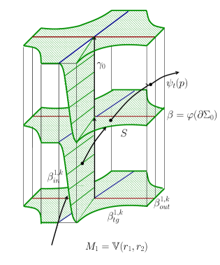
Figure 21: Local Birkhoff $S$ section around $\gamma_{0}\subset\mathbb{V}(r_{1},r_{2})$.

In the complement of $\gamma_{0}$ the surface $S$ is transverse to the vector field $X_{1}$. To see this, recall that $X_{1}$ is defined to be the vectorfield $(x,y,z)\mapsto\left(\log(\lambda)x,-\log(\lambda)y,{1}/{n}\right)$ in $\mathbb{R}^{2}\times\mathbb{R}/\mathbb{Z}.$ Since the third component is nowhere zero, it follows that it is transverse to $S$ along the horizontal parts. For the transversality along the bands, consider a point $p=(r_{1},r,s)\in S\cap A_{in}^{1}$. On $A_{in}^{1}$ there is a parametrization $r\mapsto\beta(r)=\left(r_{1},r,z_{0}+(|m|/n)\cdot\rho(r/r_{2})\right)$, where $z_{0}$ is some constant. From the definition of $S$ we have that $T_{p}S$ is generated by the vectors

$$\frac{\partial}{\partial r}(p)=(0,1,-\kappa(r))\ \ \text{and}\ \ \frac{\partial}{\partial\theta}(p)=(r_{1},r,0),$$

where $\kappa(r)=\frac{|m|}{n}|\rho^{\prime}(r/r_{2})|\geq 0.$ It follows that

$$X_{1}(p)\wedge\frac{\partial}{\partial r}(p)\wedge\frac{\partial}{\partial\theta}(p)=\begin{vmatrix}\log(\lambda)r_{1}&0&r_{1}\\ -\log(\lambda)r&1&r\\ 1/n&-\kappa(r)&0\end{vmatrix}=-\frac{r_{1}}{n}+2\kappa(r)\log(\lambda)r_{1}r$$

is strictly lower that zero, so we conclude that $X_{1}$ is transverse to $TS$ along the the arc $\beta_{in}^{1+4j}$. Then, since the surface $S$ is the image of a $1$-parameter family of horizontal homotheties $(x,y,z)\mapsto(\theta x,\theta y,z),$ and since $X_{1}$ is invariant under these transformations, this implies the transversality of $X_{1}$ with $TS$ along all the interior of the band.

By construction the surface $S$ is orientable, and it is not hard to see that $X_{1}$ traverse each band or horizontal surface always in the same sense. Thus, the orbits of $\psi_{t}$ are everywhere (topologically) transverse to the interior of $S$. In a meridian/longitude basis $\{a,b\}$ of $H_{1}(M_{1}\backslash\gamma_{0})$ the homological coordinates of $\beta$ are $[\beta]=n(\gamma,\Sigma)\cdot a+m(\gamma,\Sigma)\cdot b$, from where we deduce the linking number and multiplicity of $S$. Since $n(\gamma,\Sigma)\neq 0$, there exists a tubular neighbourhood $O$ of $\gamma_{0}$ such that every point in $O$ intersects the surface $S$ in a uniformly bounded time. Therefore, $S$ is a local Birkhoff section at $\gamma_{0}$. This completes the claim. ∎

To complete the lemma, consider the set $\Sigma^{\prime}\coloneqq\Sigma_{0}\cup S$ that is contained in $N$. Then $\Sigma^{\prime}$ is the image of a continuous immersion $\zeta:\Sigma\to N$, which is an embedding on $\mathring{\Sigma}$ and coincides with $\iota$ over $\Sigma_{0}$. From the construction it can be seen that its interior $\mathring{\Sigma}^{\prime}=\Sigma^{\prime}\backslash\partial\Sigma^{\prime}$ is (topologically) transverse to the flow lines. To prove that this is actually a Birkhoff section, it rest to show that all the $\psi_{t}$-orbits intersect $\Sigma^{\prime}$ in a uniformly bounded time. For this, consider two tubular neighbourhoods $O_{1}\subset O_{0}\subset N$ of $\gamma_{0}$ satisfying that $M_{0}\cap M_{1}$ is contained in the interior of $O_{0}\backslash O_{1}$, and that there exists $T_{1},T_{0}>0$ such that $[p,\psi_{T_{1}}(p)]\cap S\neq\emptyset$ for every $p\in O_{1}$ and $[p,\psi_{T_{0}}(p)]\cap\Sigma_{0}\neq\emptyset$ for every $p\in N\backslash O_{0}$. Then, since the neighbourhoods $O_{1}\subset O_{0}$ are nested germs of a saddle type periodic orbit, we see that there exits some $T_{2}>0$ such that $[p,\psi_{T_{2}}(p)]$ is not contained in $O_{0}\backslash O_{1}$, for every $p\in O_{0}\backslash O_{1}$. Then, taking $T>\max\{T_{0}+T_{2},T_{1}+T_{2}\}$, we deduce that $[p,\psi_{T}(p)]\cap\Sigma^{\prime}\neq\emptyset$, for every $p\in N$. This completes the lemma. ∎

For the next statement, it is convenient to consider $\Sigma$ as a fixed compact surface, for which we have two immersions $\iota:(\Sigma,\partial\Sigma)\to(M,\gamma)$ and $\zeta:(\Sigma,\partial\Sigma)\to(N,\gamma_{0})$, that are Birkhoff sections for $(\phi_{t},M)$ and $(\psi_{t},N)$, respectively. Denote by $P:\mathring{\Sigma}\to\mathring{\Sigma}$ and $P^{\prime}:\mathring{\Sigma}\to\mathring{\Sigma}$ the corresponding first return maps.

Lemma 5.19.

The homeomorphisms $P$ and $P^{\prime}$ define the same action on $\pi_{1}(\mathring{\Sigma})$.

Proof.

By construction, both flows $\phi_{t}:M\to M$ and $\psi_{t}:N\to N$ induce the same foliation by orbit segments in $M_{0}$. Moreover, if $p\in M_{0}$ and $t\geq 0$ satisfy that $[p,\psi_{t}(p)]\subset M_{0}$ or $[p,\phi_{t}(p)]\subset M_{0}$ then $\psi_{s}(p)=\phi_{s}(p)$, for $0\leq s\leq t$. Let $U\subset\Sigma_{0}$ be a collar neighbourhood of $\partial\Sigma_{0}$ and consider the subsurface $\Sigma_{U}=\Sigma_{0}\backslash U$. If we take $U$ big enough, then it is satisfied that every point $p\in\Sigma_{U}$ has a first return $\psi_{\tau}(p)\in\textsl{int}(\Sigma_{0})$ and all the orbit segment $[p,\psi_{\tau}(p)]$ is contained in $M_{0}$. Therefore, $P(p)=P^{\prime}(p)$, for every $p\in\Sigma_{U}$.

Since there is a deformation retraction $\Sigma\to\Sigma_{0}\to\Sigma_{U}$, every homotopy class $[\alpha]$ in $\pi_{1}(\Sigma)$ has a representative $\alpha_{0}\subset\Sigma_{U}$, and from the previous paragraph it follows that $P(\alpha_{0})=P^{\prime}(\alpha_{0})$. Thus, $P_{*}([\alpha])=P_{*}^{\prime}([\alpha])$, for every $[\alpha]\in\pi_{1}(\Sigma)$. ∎

Proof of proposition 5.17..

Choose $0<r_{2}<r_{1}$ small enough such that $\psi_{t}:N\to N$ is Anosov. Following lemma 5.18 above, we have two topological Anosov flows $(\phi_{t},M)$ and $(\psi_{t},N)$ equipped with Birkhoff sections $\iota:(\Sigma,\partial\Sigma)\to(M,\gamma)$ and $\zeta:(\Sigma,\partial\Sigma)\to(N,\gamma_{0})$ respectively. By construction $n(\gamma,\Sigma)=n(\gamma_{0},\Sigma^{\prime})$, $m(\gamma,\Sigma)=m(\gamma_{0},\Sigma^{\prime})$ and $p(\gamma,\Sigma)=p(\gamma_{0},\Sigma^{\prime})$. By lemma 5.19 the identity map on $\Sigma$ conjugates the corresponding first return actions on fundamental groups, so we are in the hypothesis of theorem B. We conclude that $(\phi_{t},M)$ and $(\psi_{t},N)$ are orbitally equivalent flows. ∎

References

- [1] N. Aoki and K. Hiraide. Topological theory of dynamical systems, volume 52 of North-Holland Mathematical Library. North-Holland Publishing Co., Amsterdam, 1994. Recent advances.
- [2] Christian Bonatti and Nancy Guelman. Axiom A diffeomorphisms derived from Anosov flows. J. Mod. Dyn., 4(1):1–63, 2010.
- [3] Christian Bonatti and Amie Wilkinson. Transitive partially hyperbolic diffeomorphisms on 3-manifolds. Topology, 44(3):475–508, 2005.
- [4] Marco Brunella. Expansive flows on three - manifolds. PhD thesis, SISSA, Trieste, 1992.
- [5] Marco Brunella. On the topological equivalence between Anosov flows on three-manifolds. Comment. Math. Helv., 67(3):459–470, 1992.
- [6] Marco Brunella. Expansive flows on Seifert manifolds and on torus bundles. Bol. Soc. Brasil. Mat. (N.S.), 24(1):89–104, 1993.
- [7] Wellington de Mello. Topologia das variedades. IMPA.
- [8] F. T. Farrell and L. E. Jones. Anosov diffeomorphisms constructed from . Topology, 17(3):273–282, 1978.
- [9] Albert Fathi, François Laudenbach, and Valentin Poénaru. Thurston’s work on surfaces, volume 48 of Mathematical Notes. Princeton University Press, Princeton, NJ, 2012. Translated from the 1979 French original by Djun M. Kim and Dan Margalit.
- [10] Sérgio R. Fenley. Anosov flows in -manifolds. Ann. of Math. (2), 139(1):79–115, 1994.
- [11] David Fried. Transitive Anosov flows and pseudo-Anosov maps. Topology, 22(3):299–303, 1983.
- [12] Marlies Gerber and Anatole Katok. Smooth models of Thurston’s pseudo-Anosov maps. Ann. Sci. École Norm. Sup. (4), 15(1):173–204, 1982.
- [13] Étienne Ghys. Flots d’Anosov sur les -variétés fibrées en cercles. Ergodic Theory Dynam. Systems, 4(1):67–80, 1984.
- [14] Sue Goodman. Dehn surgery on Anosov flows. In Geometric dynamics (Rio de Janeiro, 1981), volume 1007 of Lecture Notes in Math., pages 300–307. Springer, Berlin, 1983.
- [15] Michael Handel and William P. Thurston. Anosov flows on new three manifolds. Invent. Math., 59(2):95–103, 1980.
- [16] Koichi Hiraide. Expansive homeomorphisms of compact surfaces are pseudo-Anosov. Osaka J. Math., 27(1):117–162, 1990.
- [17] Takashi Inaba and Shigenori Matsumoto. Nonsingular expansive flows on -manifolds and foliations with circle prong singularities. Japan. J. Math. (N.S.), 16(2):329–340, 1990.
- [18] Anatole Katok and Boris Hasselblatt. Introduction to the modern theory of dynamical systems, volume 54 of Encyclopedia of Mathematics and its Applications. Cambridge University Press, Cambridge, 1995. With a supplementary chapter by Katok and Leonardo Mendoza.
- [19] Jorge Lewowicz. Expansive homeomorphisms of surfaces. Bol. Soc. Brasil. Mat. (N.S.), 20(1):113–133, 1989.
- [20] Jorge Lewowicz and Eduardo Lima de Sá. Analytic models of pseudo-Anosov maps. Ergodic Theory Dynam. Systems, 6(3):385–392, 1986.
- [21] Lee Mosher. Laminations and flows transverse to finite depht foliations (preprint), 1996.
- [22] Miguel Paternain. Expansive flows and the fundamental group. Bol. Soc. Brasil. Mat. (N.S.), 24(2):179–199, 1993.
- [23] Miguel Paternain. Expansive geodesic flows on surfaces. Ergodic Theory Dynam. Systems, 13(1):153–165, 1993.
- [24] J. F. Plante. Anosov flows, transversely affine foliations, and a conjecture of Verjovsky. J. London Math. Soc. (2), 23(2):359–362, 1981.
- [25] Mario Shannon. Dehn surgeries and smooth structures on 3-dimensional transitive Anosov flows. PhD thesis, Université de Bourgogne, 2020.