Malaise and remedy of binary boson-star initial data

Abstract

Through numerical simulations of boson-star head-on collisions, we explore the quality of binary initial data obtained from the superposition of single-star spacetimes. Our results demonstrate that evolutions starting from a plain superposition of individual boosted boson-star spacetimes are vulnerable to significant unphysical artefacts. These difficulties can be overcome with a simple modification of the initial data suggested in [1] for collisions of oscillatons. While we specifically consider massive complex scalar field boson star models up to a 6th-order-polynomial potential, we argue that this vulnerability is universal and present in other kinds of exotic compact systems and hence needs to be addressed.

1 Introduction

The rise of gravitational-wave (GW) physics as an observational field, marked by the detection of GW150914 [2] and followed by about 50 further compact binary events [3, 4] over the past years, has opened up unprecedented opportunities to explore gravitational phenomena. From tests of general relativity [5, 6, 7, 8, 9, 10] to the exploration of BH populations [11, 12, 13, 14, 15] or charting the universe with independent new methods [16, 17], GW astronomy offers potential for revolutionary insight into long-standing open questions; for a review see [18]. Some answers, such as the association of a soft gamma-ray burst with the neutron star merger GW170817 [19, 20] have already raised our understanding to new levels. GW physics furthermore establishes new concrete links to other fields of research, most notably to particle and high-energy physics and the exploration of the dark sector of the universe [21, 18]. Two important ingredients of this remarkable connection are the characteristic interaction of fundamental fields with compact objects through superradiance [22] and their capacity to form compact objects through an elaborate balance between the intrinsically dispersive character of the fields and their self-gravitation. The latter feature has given rise to the hypothesis of a distinct class of compact objects as early as the 1950s [23]. In contrast to their well known fermionic counterparts – stars, white dwarfs or neutron stars – these compact objects are composed of bosonic particles or fields and, hence, commonly referred to as Boson Stars (BS). GW observations provide the first systematic approach to search for populations of these objects or to constrain their abundance. As with all other GW explorations, the success of this exploration is heavily reliant on the availability of accurate theoretical predictions for the anticipated GW signals. This type of calculation, using numerical relativity techniques [24], is the topic of this work.

The idea of bosonic stars dates back to Wheeler’s 1955 study of gravitational-electromagnetic entities or geons [23]. By generalising from real to complex-valued fundamental fields, it is even possible to obtain genuinely stationary solutions to the Einstein-matter equations. First established for spin 0 or scalar fields [25, 26, 27], this idea has more recently been extended to spin 1 or vector (aka Proca) fields [28] as well as wider classes of scalar BSs [29, 30]. In the wake of the dramatic progress of numerical relativity in the simulations of black holes (BHs) [31, 32, 33] (see [34] for a review), the modelling of BSs and binary systems involving BSs has rapidly gathered pace.

The first BS models computed in the 1960s consisted of a massive but non-interacting complex scalar field $\varphi$. This class of stationary BSs, commonly referred to as mini boson stars, consists of a one parameter family of ground-state solutions characterised by the central scalar-field amplitude that reveals a stability structure analogous to that of Tolman-Oppenheimer-Volkoff [35, 36] stars: a stable and an unstable branch of ground-state solutions are separated by the configuration with maximal mass [37, 38, 39]. For each ground-state model, there furthermore exists a countable hierarchy of excited states with $n>0$ nodes in the scalar profile [40, 41, 42]. Numerical evolutions of these excited BSs demonstrate their unstable character, but also reveal significant variation in the instability time scales [43].

Whereas mini BS models are limited in terms of their maximum compactness, self-interacting scalar fields can result in significantly more compact stars, even denser than neutron stars [44, 45, 46, 47]. This raises the intriguing question whether compact BS binaries may reveal themselves through characteristic GW emission analogous to that from BHs or NSs [48]. Recent studies conclude that this may well be within the grasp of next-generation GW detectors and, in the case of favourable events, even with advanced LIGO [49, 50, 51].

One of the characteristic properties of BSs is the quantised nature of their spin. The linearised Einstein equations in the slow-rotation limit lead to a two-dimensional Poisson equation that does not admit everywhere regular solutions except for trivial constants; in consequence BSs cannot rotate perturbatively [52]. By relaxing the slow-rotation approximation, Schunck and Mielke [53] computed the first (differentially) rotating BSs and found that these solutions have an integer ratio of angular momentum to particle number. The structure of spinning BS models has been studied extensively over the years [54, 55, 56, 57, 58, 59, 60, 61, 62]. The quantised nature of the angular momentum also applies to Proca and Dirac (spin $\tfrac{1}{2}$) stars [63], but numerical studies of the formation of rotating stars have revealed a striking difference between the scalar and vector case: while collapsing scalar fields shed all their angular momentum through an axisymmetric instability, the collapse of vector fields results in spinning Proca stars with no indication of an instability [64, 50]. This observation is supported by analytic calculations [65], but the instability may be quenched by self-interaction terms in the potential function or in the Newtonian limit [66]. For further reviews of the structure and dynamics of single BSs, we note the reviews [67, 68, 69, 70].

The first simulations of BS binaries have considered the head-on collision of configurations with phase differences between the constituent stars or opposite frequencies [71]; see also [72, 73]. The phase or frequency differences manifest themselves most pronouncedly in the dynamics and GW emission at late times around merger. These collisions result in either a BH, a non-rotating BS or a near-annihilation of the scalar field in the case of opposite frequencies. BS binaries with orbital angular momentum generate a GW signal qualitatively similar to that of BH binaries during the inspiral phase, but exhibit a much more complex structure around merger [74, 75]. In agreement with the above mentioned BS formation studies, the BS inspirals also seem to avoid the formation of spinning BSs, although they may settle down into single nonrotating BSs.

In spite of the rapid progress of this field, the computation of GW templates for BSs still lags considerably behind that of BH binaries, both in terms of precision and coverage of the parameter space. Clearly, the presence of the matter fields adds complexity to this challenge, but also alleviates some of the difficulties through the non-singular character of the BS spacetimes. The first main goal of our study is to highlight the substantial risk of obtaining spurious physical results due to the use of overly simplistic initial data constructed by plain superposition of single-BS spacetimes. Our second main goal is to demonstrate how an astonishingly simple modification of the superposition procedure, first identified by Helfer et al. [1] for oscillatons, overcomes most of the problems encountered with plain superposition. We summarise our main findings as follows.

• An adjustment of the superposition procedure, given by Eq. (45), results in a significant reduction of the constraint violations inherent to the initial data; see Fig. 3.

• In the head-on collision of mini BS binaries with rather low compactness, we observe a significant drop of the radiated GW energy with increasing distance $d$ if we use plain superposition. This physically unexpected dependence on the initial separation levels off only for rather large $d\gtrsim 150\,M$, where $M$ denotes the Arnowitt-Deser-Misner (ADM) mass [76]. In contrast, the total radiated energy computed from the evolution of our adjusted initial data displays the expected behaviour over the entire studied range $75.5\,M\leq d\leq 176\,M$: a very mild increase in the radiated energy with $d$. In the limit of large $d\gtrsim 150\,M$, both types of simulations agree within numerical uncertainties; see upper panel in Fig. 6.

• In collisions of highly compact BSs with solitonic potentials, the radiated energy is largely independent of the initial separations for both initial data types, but for plain superposition we consistently obtain $\sim 10\,\%$ more radiation than for the adjusted initial data; see bottom panel in Fig. 6. Furthermore, we find plain superposition to result in a slightly faster infall. The most dramatic difference, however, is the collapse into individual BHs of both BSs well before merger if we use plain superposition. No such collapse occurs if we use adjusted initial data. Rather, these lead to the expected near-constancy of the central scalar-field amplitude of the BSs throughout most of the infall; see Fig. 9.

• We have verified through evolutions of single boosted BSs that the premature collapse into a BH is closely related to the spurious metric perturbation (44) that arises in the plain superposition procedure. Artificially adding the same perturbation to a single BS spacetime induces an unphysical collapse of the BS that is in qualitative and quantitative agreement with that observed in the binary evolution starting with plain superposition; see Fig. 9.

The detailed derivation of these results begins in Sec. 2 with a review of the formalism and the computational framework of our BS simulations. We discuss in more detail in Sec. 3 the construction of initial data through plain superposition and our modification of this method. In Sec. 4, we compare the dynamics of head-on collisions of mini BSs and highly compact solitonic BS binaries starting from both types of initial data. We note the substantial differences in the results thus obtained and argue why we regard the results obtained with our modification to be correct within numerical uncertainties. We summarise our findings and discuss future extensions of this work in Sec. 5.

Throughout this work, we use units where the speed of light and Planck’s constant are set to unity, $c=\hbar=1$. We denote spacetime indices by Greek letters running from 0 to 3 and spatial indices by Latin indices running from 1 to 3.

2 Formalism

2.1 Action and covariant field equations

The action for a complex scalar field $\varphi$ minimally coupled to gravity is given by

$$S=\int\sqrt{-g}\left\{\frac{1}{16\pi G}R-\frac{1}{2}\left[g^{\mu\nu}\nabla_{\mu}\bar{\varphi}\nabla_{\nu}\varphi+V(\varphi)\right]\right\}\mathrm{d}^{4}x\,,$$ (1)

where $g_{\alpha\beta}$ denotes the spacetime metric and $R$ the Ricci scalar associated with this metric. The characteristics of the resulting BS models depend on the scalar potential $V(\varphi)$; in this work, we consider mini boson stars and solitonic boson stars, obtained respectively for the potential functions

$$V_{\rm min}=\mu^{2}|\varphi|^{2}\,,~{}~{}~{}~{}~{}~{}~{}~{}~{}~{}V_{\rm sol}=\mu^{2}|\varphi|^{2}\left(1-2\frac{|\varphi|^{2}}{\sigma_{0}^{2}}\right)^{2}\,.$$ (2)

Here, $\mu$ denotes the mass of the scalar field and $\sigma_{0}$ describes the self-interaction in the solitonic potential which can result in highly compact stars [45]. Note that $V_{\rm sol}\rightarrow V_{\rm min}$ in the limit $\sigma_{0}\rightarrow\infty$.

Variation of the action (1) with respect to the metric and the scalar field yield the Einstein and matter evolution equations

$$G_{\alpha\beta}=8\pi GT_{\alpha\beta}=8\pi G\left[\partial_{(\alpha}\bar{\varphi}\partial_{\beta)}\varphi-\frac{1}{2}g_{\alpha\beta}\big{(}g^{\mu\nu}\partial_{\mu}\bar{\varphi}\partial_{\nu}\varphi+V(\varphi)\big{)}\right]\,,$$ (3)

$$\nabla^{\mu}\nabla_{\mu}\varphi=\varphi V^{\prime}\mathrel{\vbox{\hbox{\scriptsize.}\hbox{\scriptsize.}}}=\varphi\frac{\mathrm{d}}{\mathrm{d}|\varphi|^{2}}V\,.$$ (4)

Readers who are mainly interested in the results of our work and/or are familiar with the equations governing BS spacetimes may proceed directly to Sec. 3.

2.2 3+1 formulation

For all simulations performed in this work, we employ the 3+1 spacetime split of ADM [76] and York [77]; see also [78]. Here, the spacetime metric is decomposed into the physical 3-metric $\gamma_{ij}$, the shift vector $\beta^{i}$ and the lapse function $\alpha$ according to

$$\mathrm{d}s^{2}=g_{\alpha\beta}\mathrm{d}x^{\alpha}\mathrm{d}x^{\beta}=-\alpha^{2}\mathrm{d}t^{2}+\gamma_{mn}(\mathrm{d}x^{m}+\beta^{m}\mathrm{d}t)(\mathrm{d}x^{n}+\beta^{n}\mathrm{d}t)\,,$$ (5)

where the level sets $x^{0}=t=\mathrm{const}$ represent three-dimensional spatial hypersurfaces with timelike unit normal $n_{\mu}$. Defining the extrinsic curvature

$$K_{ij}=-\frac{1}{2\alpha}(\partial_{t}\gamma_{ij}-\beta^{m}\partial_{m}\gamma_{ij}-\gamma_{im}\partial_{j}\beta^{m}-\gamma_{mj}\partial_{i}\beta^{m})\,,$$ (6)

the Einstein equations result in a first-order-in-time set of differential equations for $\gamma_{ij}$ and $K_{ij}$ that is readily converted into the conformal Baumgarte-Shapiro-Shibata-Nakamura-Oohara-Kojima (BSSNOK) formulation [79, 80, 81]. More specifically, we define

$$\chi=\gamma^{-1/3}\,,~{}~{}~{}~{}K=\gamma^{mn}K_{mn}\,,~{}~{}~{}~{}\tilde{\gamma}_{ij}=\chi\gamma_{ij}\,,$$

$$\tilde{A}_{ij}=\chi\left(K_{ij}-\frac{1}{3}\gamma_{ij}K\right)\,,~{}~{}~{}~{}\tilde{\Gamma}^{i}=\tilde{\gamma}^{mn}\tilde{\Gamma}^{i}_{mn}\,,$$ (7)

where $\gamma=\det\gamma_{ij}$, and $\tilde{\Gamma}^{i}_{mn}$ are the Christoffel symbols associated with $\tilde{\gamma}_{ij}$. The Einstein equations are then given by (see for example Sec. 6 in [21] for more details)

$$\partial_{t}\chi =\beta^{m}\partial_{m}\chi+\frac{2}{3}\chi(\alpha K-\partial_{m}\beta^{m})\,,$$ (8)

$$\partial_{t}\tilde{\gamma}_{ij} =\beta^{m}\partial_{m}\tilde{\gamma}_{ij}+2\tilde{\gamma}_{m(i}\partial_{j)}\beta^{m}-\frac{2}{3}\tilde{\gamma}_{ij}\partial_{m}\beta^{m}-2\alpha\tilde{A}_{ij}\,,$$ (9)

$$\partial_{t}K =\beta^{m}\partial_{m}K-\chi\tilde{\gamma}^{mn}D_{m}D_{n}\alpha+\alpha\tilde{A}^{mn}\tilde{A}_{mn}+\frac{1}{3}\alpha K^{2}+4\pi G\alpha(S+\rho)\,,$$ (10)

$$\partial_{t}\tilde{A}_{ij} =\beta^{m}\partial_{m}\tilde{A}_{ij}+2\tilde{A}_{m(i}\partial_{j)}\beta^{m}-\frac{2}{3}\tilde{A}_{ij}\partial_{m}\beta^{m}+\alpha K\tilde{A}_{ij}-2\alpha\tilde{A}_{im}\tilde{A}^{m}{}_{j}$$

$$~{}~{}+\chi(\alpha\mathcal{R}_{ij}-D_{i}D_{j}\alpha-8\pi G\alpha S_{ij})^{\rm TF}\,,$$ (11)

$$\partial_{t}\tilde{\Gamma}^{i} =\beta^{m}\partial_{m}\tilde{\Gamma}^{i}+\frac{2}{3}\tilde{\Gamma}^{i}\partial_{m}\beta^{m}-\tilde{\Gamma}^{m}\partial_{m}\beta^{i}+\tilde{\gamma}^{mn}\partial_{m}\partial_{n}\beta^{i}+\frac{1}{3}\tilde{\gamma}^{im}\partial_{m}\partial_{n}\beta^{n}$$

$$~{}~{}~{}-\tilde{A}^{im}\left(3\alpha\frac{\partial_{m}\chi}{\chi}+2\partial_{m}\alpha\right)+2\alpha\tilde{\Gamma}^{i}_{mn}\tilde{A}^{mn}-\frac{4}{3}\alpha\tilde{\gamma}^{im}\partial_{m}K-16\pi G\frac{\alpha}{\chi}j^{i}\,,$$ (12)

where ‘TF’ denotes the trace-free part and auxiliary expressions are given by

$$\Gamma^{i}_{jk} =\tilde{\Gamma}^{i}_{jk}-\frac{1}{2\chi}(\delta^{i}{}_{k}\partial_{j}\chi+\delta^{i}{}_{j}\partial_{k}\chi-\tilde{\gamma}_{jk}\tilde{\gamma}^{im}\partial_{m}\chi)\,,$$

$$\mathcal{R}_{ij} =\tilde{R}_{ij}+\mathcal{R}^{\chi}_{ij}\,,$$

$$\mathcal{R}^{\chi}_{ij} =\frac{\tilde{\gamma}_{ij}}{2\chi}\left[\tilde{\gamma}^{mn}\tilde{D}_{m}\tilde{D}_{n}\chi-\frac{3}{2\chi}\tilde{\gamma}^{mn}\partial_{m}\chi\,\partial_{n}\chi\right]+\frac{1}{2\chi}\left(\tilde{D}_{i}\tilde{D}_{j}\chi-\frac{1}{2\chi}\partial_{i}\chi\,\partial_{j}\chi\right)\,,$$

$$\tilde{R}_{ij} =-\frac{1}{2}\tilde{\gamma}^{mn}\partial_{m}\partial_{n}\tilde{\gamma}_{ij}+\tilde{\gamma}_{m(i}\partial_{j)}\tilde{\Gamma}^{m}+\tilde{\Gamma}^{m}\tilde{\Gamma}_{(ij)m}+\tilde{\gamma}^{mn}\left[2\tilde{\Gamma}^{k}_{m(i}\tilde{\Gamma}_{j)kn}+\tilde{\Gamma}^{k}_{im}\tilde{\Gamma}_{kjn}\right]\,,$$

$$D_{i}D_{j}\alpha =\tilde{D}_{i}\tilde{D}_{j}\alpha+\frac{1}{\chi}\partial_{(i}\chi\partial_{j)}\alpha-\frac{1}{2\chi}\tilde{\gamma}_{ij}\tilde{\gamma}^{mn}\partial_{m}\chi\,\partial_{n}\alpha\,.$$ (13)

Here, $\tilde{D}$ and $\tilde{\mathcal{R}}$ denote the covariant derivative and the Ricci tensor of the conformal metric $\tilde{\gamma}_{ij}$, respectively.

The matter terms in Eqs. (8)-(12) are defined by

$$\rho=T_{\mu\nu}n^{\mu}n^{\nu}\,,~{}~{}~{}j_{\alpha}=-\bot^{\nu}{}_{\alpha}T_{\mu\nu}n^{\mu}\,,~{}~{}~{}S_{\alpha\beta}=\bot^{\mu}{}_{\alpha}\bot^{\nu}{}_{\beta}T_{\mu\nu}\,,~{}~{}~{}\bot^{\mu}{}_{\alpha}=\delta^{\mu}{}_{\alpha}+n^{\mu}n_{\alpha}\,.$$ (14)

In adapted coordinates, we only need $\rho$ and the spatial components $j^{i}$, $S_{ij}$ which are determined by the scalar field through Eq. (3), Defining, in analogy to the extrinsic curvature (6),

$$\Pi=-\frac{1}{2\alpha}(\partial_{t}\varphi-\beta^{m}\partial_{m}\varphi)~{}~{}~{}~{}~{}\Leftrightarrow~{}~{}~{}~{}~{}\partial_{t}\varphi=\beta^{m}\partial_{m}\varphi-2\alpha\Pi\,,$$ (15)

we obtain

$$\rho = 2\Pi\,\bar{\Pi}+\frac{1}{2}\partial^{m}\bar{\varphi}\,\partial_{m}\varphi+\frac{1}{2}V\,,~{}~{}~{}~{}~{}S+\rho=8\bar{\Pi}\,\Pi-V\,,$$

$$j_{i} = \bar{\Pi}\partial_{i}\varphi+\Pi\partial_{i}\bar{\varphi}\,,$$

$$S_{ij} = \partial_{(i}\bar{\varphi}\partial_{j)}\varphi-\frac{1}{2}\gamma_{ij}\left(\gamma^{mn}\partial_{m}\bar{\varphi}\,\partial_{n}\varphi-4\bar{\Pi}\,\Pi+V\right)\,.$$ (16)

The evolution of the scalar field according to Eq. (4) in terms of our 3+1 variables is given by Eq. (15) and

$$\partial_{t}\Pi=\beta^{m}\partial_{m}\Pi+\alpha\left[\Pi K+\frac{1}{2}V^{\prime}\varphi+\frac{1}{4}\tilde{\gamma}^{mn}\left(\partial_{m}\varphi\partial_{n}\chi-2\chi\tilde{D}_{m}\tilde{D}_{n}\varphi\right)\right]-\frac{1}{2}\chi\tilde{\gamma}^{mn}\partial_{m}\varphi\partial_{n}\alpha\,,$$ (17)

where $V^{\prime}=\mathrm{d}V/\mathrm{d}(|\varphi|^{2})$

Finally, we evolve the gauge variables $\alpha$ and $\beta^{i}$ with 1+log slicing and the $\Gamma$-driver condition (the so-called moving puncture conditions [32, 33]),

$$\partial_{t}\alpha=\beta^{m}\partial_{m}\alpha-2\alpha K\,,~{}~{}~{}\partial_{t}\beta^{i}=\beta^{m}\partial_{m}\beta^{i}+\frac{3}{4}B^{i}\,,~{}~{}~{}\partial_{t}B^{i}=\beta^{m}\partial_{m}B^{i}+\partial_{t}\tilde{\Gamma}^{i}-\eta B^{i}\,,$$ (18)

where $\eta$ is a constant we typically set to $M\eta\approx 1$ in units of the ADM mass $M$.

Additionally to the evolution equations (8)-(12), the Einstein equations also imply four equations that do not contain time derivatives, the Hamiltonian and momentum constraints

$$\mathcal{H}\mathrel{\vbox{\hbox{\scriptsize.}\hbox{\scriptsize.}}}=\mathcal{R}+K^{2}-K^{mn}K_{mn}-16\pi\rho=0\,,$$ (19)

$$\mathcal{M}_{i}\mathrel{\vbox{\hbox{\scriptsize.}\hbox{\scriptsize.}}}=D_{i}K-D_{m}K^{m}{}_{i}+8\pi j_{i}=0\,.$$ (20)

While the constraints are preserved under time evolution in the continuum limit, some level of violations is inevitable due to numerical noise or imperfections of the initial data. We will return to this point in more detail in Sec. 3 below.

For the time evolutions discussed in Sec. 4, we have implemented the equations of this section in the lean code [82] which is based on the cactus computational toolkit [83]. The equations are integrated in time with the method of lines using the fourth-order Runge-Kutta scheme with a Courant factor $1/4$ and fourth-order spatial discretisation. Mesh refinement is provided by carpet [84] in the form of “moving boxes” and we compute apparent horizons with AHFinderDirect [85, 86].

2.3 Stationary boson stars and initial data

The initial data for our time evolution are based on single stationary BS solutions in spherical symmetry. Using spherical polar coordinates, areal radius and polar slicing, the line element can be written as

$$\mathrm{d}s^{2}=-e^{2\Phi}\mathrm{d}t^{2}+\left(1-\frac{2m}{r}\right)^{-1}\mathrm{d}r^{2}+r^{2}(\mathrm{d}\theta^{2}+\sin^{2}\theta\mathrm{d}\phi^{2})\,.$$ (21)

where $\Phi$ and $m$ are functions of $r$ only. It turns out convenient to express the complex scalar field in terms of amplitude and frequency,

$$\varphi(t,r)=A(r)e^{\mathrm{i}\mkern 1.0mu\omega t}\,,~{}~{}~{}~{}~{}\omega=\mathrm{const}\in\mathbb{R}\,.$$ (22)

At this point, our configurations are characterised by two scales, the scalar mass $\mu$ and the gravitational constant $G$. In the following, we absorb $\mu$ and $G$ by rescaling all dimensional variables according to

$$\hat{t}=\mu t\,,~{}~{}~{}\hat{r}=\mu r\,,~{}~{}~{}\hat{m}=\mu m\,,~{}~{}~{}\hat{A}=\sqrt{G}A\,,~{}~{}~{}\hat{\omega}=\omega/\mu\,;$$ (23)

note that $\mu$ has the dimension of a frequency or wave number and $\sqrt{G}$ is an inverse mass. Using the Planck mass $M_{\rm Pl}=1/\sqrt{G}=1.221\times 10^{19}\,{\rm GeV}$, we can restore SI units from the dimensionless numerical variables according to

$$r=\hat{r}\times\left(\frac{\mu}{1.937\times 10^{-10}\,{\rm eV}}\right)^{-1}\,{\rm km}\,,~{}~{}~{}\omega=\hat{\omega}\times\frac{\mu}{6.582\times 10^{-16}\,{\rm eV}}\,{\rm Hz}\,,~{}~{}~{}A=\hat{A}\,M_{\rm Pl}\,,$$

and likewise for other variables. The rescaled version of the potential (2) is given by

$$\hat{V}_{\rm min}=\hat{A}^{2}\,,~{}~{}~{}~{}~{}~{}~{}~{}~{}~{}\hat{V}_{\rm sol}=\hat{A}^{2}\left(1-2\frac{\hat{A}^{2}}{\hat{\sigma}_{0}^{2}}\right)^{2}~{}~{}\text{with}~{}~{}\hat{\sigma}_{0}=\sqrt{G}\sigma_{0}\,.$$ (24)

In terms of the rescaled variables, the Einstein-Klein-Gordon equations in spherical symmetry become

$$\partial_{\hat{r}}\Phi =\frac{\hat{m}}{\hat{r}(\hat{r}-2\hat{m})}+2\pi\hat{r}\left(\hat{\eta}^{2}+\hat{\omega}^{2}e^{-2\Phi}\hat{A}^{2}-\hat{V}\right)\,,$$ (25)

$$\partial_{\hat{r}}\hat{m} =2\pi\hat{r}^{2}\left(\hat{\eta}^{2}+\hat{\omega}^{2}e^{-2\Phi}\hat{A}^{2}+\hat{V}\right)\,,$$ (26)

$$\partial_{\hat{r}}\hat{A} =\left(1-\frac{2\hat{m}}{\hat{r}}\right)^{-1/2}\hat{\eta}\,,$$ (27)

$$\partial_{\hat{r}}\hat{\eta} =-2\frac{\hat{\eta}}{\hat{r}}-\hat{\eta}\partial_{\hat{r}}\Phi+\left(1-\frac{2\hat{m}}{\hat{r}}\right)^{-1/2}(\hat{V}^{\prime}-\hat{\omega}^{2}e^{-2\Phi})\hat{A}~{}~{}~{}\text{with}~{}~{}\hat{V}^{\prime}=\frac{\mathrm{d}\hat{V}}{\mathrm{d}(\hat{A})^{2}}\,.$$ (28)

By regularity, we have the following boundary conditions at the origin $\hat{r}=0$ and at infinity,

$$\hat{A}(0)=\hat{A}_{\rm ctr}\in\mathbb{R}^{+}\,,~{}~{}~{}~{}~{}\hat{m}(0)=0\,,~{}~{}~{}~{}~{}\hat{\eta}(0)=0\,,~{}~{}~{}~{}~{}\Phi(\infty)=0\,,~{}~{}~{}~{}~{}\hat{A}(\infty)=0\,.$$ (29)

This two-point-boundary-value problem has two free parameters, the central amplitude $\hat{A}_{\rm ctr}$ and the frequency $\hat{\omega}$. For a given value $\hat{A}_{\rm ctr}$, however, only a discrete (albeit infinite) number of frequency values $\hat{\omega}$ will result in models with $\hat{A}(\infty)=0$; all other frequencies lead to an exponentially divergent scalar field as $r\rightarrow\infty$. The “correct” frequencies are furthermore ordered by $\hat{\omega}_{n}<\hat{\omega}_{n+1}$, where $n\geq 0$ is the number of zero crossings of the scalar profile $\hat{A}(\hat{r})$; $n=0$ corresponds to the ground state and $n>0$ to the $n^{\rm th}$ excited state [43]. Finding the frequency for a regular star for user-specified $\hat{A}_{\rm ctr}$ and $n$ is the key challenge in computing BS models. We obtain these solutions through a shooting algorithm, starting with the integration of Eqs. (25)-(28) outwards for $\hat{A}(0)=\hat{A}_{\rm ctr}$ specified, $\Phi(0)=1$, and our “initial guess” $\hat{\omega}=1$. Depending on the number of zero crossings in this initial-guess model, we repeat the calculation by increasing or decreasing $\hat{\omega}$ by one order of magnitude until we have obtained an upper and a lower limit for $\hat{\omega}$. Through iterative bisection, we then rapidly converge to the correct frequency. Because we can only determine $\hat{\omega}$ to double precision, we often find it necessary to capture the scalar field behaviour at large radius by matching to its asymptotic behaviour

$$\varphi\sim\frac{1}{\hat{r}}\exp\left({-\sqrt{1-\hat{\omega}^{2}e^{-2\Phi}}}\right)\,,$$ (30)

outside a user-specified radius $\hat{r}_{\rm match}$. Finally, we can use an additive constant to shift the function $\Phi(\hat{r})$ to match its outer boundary condition. In practice, we impose this condition in the form of the Schwarzschild relation $e^{2\Phi}=(1-2\hat{m}/\hat{r})$ at the outer edge of our grid; in vacuum this is exact even at finite radius, and we can safely ignore the scalar field at this point thanks to its exponential falloff.

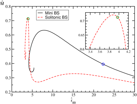
Figure 1: One parameter families of mini BSs (black solid) with a non-interacting potential $\hat{V}_{\rm min}$ and solitonic BSs (red dashed) with potential $\hat{V}_{\rm sol}$ and $\hat{\sigma}_{0}=0.2$ as given in Eq. (24). In Sec. 4 we simulate head-on collisions of two specific models marked by the circles and with parameters listed in Table 1.

For a given potential, the solutions computed with this method form a one-parameter family characterised by the central scalar field amplitude $\hat{A}_{0}$. In Fig. 1 we display two such families for the potentials (24) with $\hat{\sigma}_{0}=0.2$ in the mass-radius diagram using the areal radius $\hat{r}_{99}$ containing $99\,\%$ of the BS’s total mass. In that figure, we have also marked by circles two specific models, one mini BS and one solitonic BS, which we use in the head-on collisions in Sec. 4 below. We have chosen these two models to represent one highly compact and one rather squishy BS; note that both models are located to the right of the maximal $\hat{M}(\hat{r})$ and, hence, stable stars. Their parameters and properties are summarised in Table 1.

Model	$\sqrt{G}A_{\rm ctr}$	$\sqrt{G}\sigma_{0}$	$\mu M_{\rm BS}$	$\omega/\mu$	$\mu r_{99}$	$\max\frac{m(r)}{r}$
mini	0.0124	$\infty$	$0.395$	$0.971$	$22.31$	$0.0249$
soli	0.17	$0.2$	$0.713$	$0.439$	$3.98$	$0.222$

Table 1: Parameters of the two single, spherically symmetric ground state BS models employed for our simulations of head-on collisions. Up to the rescaling with the scalar mass $\mu$, each BS is determined by the central amplitude $A_{\rm ctr}$ of the scalar field and the potential parameter $\sigma_{0}$ of Eq. (2). The mass $M_{\rm BS}$ of the boson star, the scalar field frequency $\omega$, the areal radius $r_{99}$ containing $99\,\%$ of the total mass $M_{\rm BS}$ and the compactness, defined here as the maximal ratio of the mass function to radius, represent the main features of the stellar model.

The formalism discussed so far provides us with BS solutions in radial gauge and polar slicing. In order to reduce the degree of gauge adjustment in our moving puncture time evolutions, however, we prefer using conformally flat BS models in isotropic gauge. In isotropic coordinates, the line element of a spherically symmetric spacetime has the form

$$\mu^{2}\mathrm{d}s^{2}=-e^{2\Phi}\mathrm{d}\hat{t}^{2}+\psi^{4}(\mathrm{d}\hat{R}^{2}+\hat{R}^{2}\mathrm{d}\Omega^{2})\,,$$ (31)

where $\mathrm{d}\Omega^{2}=\mathrm{d}\theta^{2}+\sin^{2}\theta\,\mathrm{d}\phi^{2}$. Comparing this with the polar-areal line element (21), we obtain two conditions,

$$\psi^{4}\hat{R}^{2}=\hat{r}^{2}\,,~{}~{}~{}~{}~{}~{}~{}~{}\psi^{4}\mathrm{d}\hat{R}^{2}=X^{2}\mathrm{d}\hat{r}^{2}~{}~{}~{}\text{with}~{}~{}~{}X=\left(1-\frac{2\hat{m}}{\hat{r}}\right)^{-1/2}\,.$$ (32)

In terms of the new variable $f(\hat{r})=\hat{R}/\hat{r}$, we obtain the differential equation

$$\frac{\mathrm{d}f}{\mathrm{d}\hat{r}}=\frac{f}{\hat{r}}(X-1)\,,$$ (33)

which we integrate outwards by assuming $\hat{R}\propto\hat{r}$ near $\hat{r}=0$. The integrated solution can be rescaled by a constant factor to ensure that at large radii – where the scalar field has dropped to a negligible level – we recover the Schwarzschild value $\psi=1+\frac{\hat{m}}{2\hat{R}}$, in accordance with Birkhoff’s theorem. Bearing in mind that $\psi^{4}\hat{R}^{2}=\hat{r}^{2}$, this directly leads to the outer boundary condition

$$\hat{R}_{\rm ob}=\frac{\hat{r}_{\rm ob}-\hat{m}_{\rm ob}}{2}\left[1+\sqrt{1-\frac{\hat{m}_{\rm ob}^{2}}{(\hat{r}_{\rm ob}-\hat{m}_{\rm ob})^{2}}}\right]\,,$$ (34)

end, hence, the overall scaling factor applied to the function $\hat{R}(\hat{r})$.

In isotropic coordinates, the resulting spacetime metric is trivially converted from spherical to Cartesian coordinates $\hat{x}^{i}=(\hat{x},\hat{y},\hat{z})$ using $\mathrm{d}\hat{R}^{2}+\hat{R}^{2}\mathrm{d}\Omega^{2}=\mathrm{d}\hat{x}^{2}+\mathrm{d}\hat{y}^{2}+\mathrm{d}\hat{z}^{2}$, so that

$$\mu^{2}\mathrm{d}s^{2}=-e^{2\Phi}\mathrm{d}\hat{t}^{2}+\psi^{4}\delta_{ij}\mathrm{d}\hat{x}^{i}\,\mathrm{d}\hat{x}^{j}\,.$$ (35)

For convenience, will drop the caret on the rescaled coordinates and variables from now on and implicitly assume that they represent dimensionless quantities to be converted into dimensional form according to Eq. (23).

2.4 Boosted boson stars

The single BS solutions can be converted into boosted stars through a straightforward Lorentz transformation. For this purpose, we denote the star’s rest frame by $\mathcal{O}$ with Cartesian 3+1 coordinates $x^{\alpha}=(t,\,x^{k})$ and consider a second frame $\tilde{\mathcal{O}}$ with Cartesian 3+1 coordinates $\tilde{x}^{\tilde{\alpha}}=(\tilde{t},\,\tilde{x}^{\tilde{k}})$ that moves relative to $\mathcal{O}$ with constant velocity $v^{i}$. These two frames are related by the transformation

$$\Lambda^{\tilde{\alpha}}{}_{\mu}=\left(\begin{array}[]{c|c}\gamma&-\gamma v_{j}\\ \hline\cr-\gamma v^{i}&\delta^{i}{}_{j}+(\gamma-1)\frac{v^{i}v_{j}}{|\boldsymbol{v}|^{2}}\end{array}\right)~{}~{}~{}~{}\Leftrightarrow~{}~{}~{}~{}\Lambda^{\mu}{}_{\tilde{\alpha}}=\left(\begin{array}[]{c|c}\gamma&\gamma v_{j}\\ \hline\cr\gamma v^{i}&\delta^{i}{}_{j}+(\gamma-1)\frac{v^{i}v_{j}}{|\boldsymbol{v}|^{2}}\end{array}\right)\,.$$

Starting with the isotropic rest-frame metric (31) and the complex scalar field $\varphi(t,R)=A(R)e^{\mathrm{i}\mkern 1.0mu\omega t+\vartheta_{0}}$ with $R=\sqrt{\delta_{mn}x^{m}x^{n}}$, we obtain a general boosted model in terms of the 3+1 variables in Cartesian coordinates $\tilde{x}^{\tilde{k}}$ as follows.

• A straightforward calculation leads to the first derivatives of the metric, its inverse and the scalar field in Cartesian coordinates $x^{i}$ in the rest frame,

  $$\partial_{t}g_{\mu\nu}=\partial_{t}g^{\mu\nu}=0\,,~{}~{}~{} \partial_{t}\varphi_{R}=-\omega\varphi_{I}\,,~{}~{}~{}\partial_{t}\varphi_{I}=\omega\varphi_{R}\,,$$

  $$\partial_{i}g_{00}=-2e^{2\Phi}\frac{\mathrm{d}\Phi}{\mathrm{d}R}\frac{x^{i}}{R}\,,~{}~{}~{}~{}~{} \partial_{i}g^{00}=2e^{-2\Phi}\frac{\mathrm{d}\Phi}{\mathrm{d}R}\frac{x^{i}}{R}\,,$$

  $$\partial_{i}g_{kk}=4\psi^{3}\frac{\mathrm{d}\psi}{\mathrm{d}R}\frac{x^{i}}{R}\,, \partial_{i}g^{kk}=-4\psi^{-5}\frac{\mathrm{d}\psi}{\mathrm{d}R}\frac{x^{i}}{R}\,,$$

  $$\partial_{i}\varphi_{R}=\frac{\eta}{f}\cos(\omega t+\phi_{0})\,\frac{x^{i}}{R}\,,~{}~{}~{}~{} \partial_{i}\varphi_{I}=\frac{\eta}{f}\sin(\omega t+\phi_{0})\,\frac{x^{i}}{R}\,,$$ (36)

  where $\varphi_{R}$ and $\varphi_{I}$ are the real and imaginary part of the scalar field, and

  $$\frac{\mathrm{d}\psi}{\mathrm{d}R}=-\frac{1}{2}\frac{X-1}{X}\frac{\psi}{R}\,,~{}~{}~{}~{}~{}\displaystyle\frac{\mathrm{d}\Phi}{\mathrm{d}R}=\frac{X^{2}-1}{2XR}+\frac{2\pi R}{f^{2}}X(\eta^{2}+\omega^{2}e^{-2\Phi}A^{2}-V)\,.$$ (37)

• We Lorentz transform the spacetime metric, the scalar field and their derivatives to the boosted frame $\tilde{\mathcal{O}}$ according to

  $$\tilde{g}_{\tilde{\alpha}\tilde{\beta}}=\Lambda^{\mu}{}_{\tilde{\alpha}}\Lambda^{\nu}{}_{\tilde{\beta}}g_{\mu\nu}\,,~{}~{}~{}\tilde{g}^{\tilde{\alpha}\tilde{\beta}}=\Lambda^{\tilde{\alpha}}{}_{\mu}\Lambda^{\tilde{\beta}}{}_{\nu}g^{\mu\nu}\,,~{}~{}~{}\partial_{\tilde{\gamma}}\tilde{g}_{\tilde{\alpha}\tilde{\beta}}=\Lambda^{\lambda}{}_{\tilde{\gamma}}\Lambda^{\mu}{}_{\tilde{\alpha}}\Lambda^{\nu}{}_{\tilde{\beta}}\partial_{\lambda}g_{\mu\nu}\,,$$

  $$\tilde{\varphi}(\tilde{x}^{\alpha})=\varphi(x^{\mu})\,,~{}~{}~{}\partial_{\tilde{\alpha}}\tilde{\varphi}=\Lambda^{\mu}{}_{\tilde{\alpha}}\partial_{\mu}\varphi\,.$$ (38)

• We construct the 3+1 variables in the boosted frame from these quantities according to

  $$\tilde{\alpha}=\left(-\tilde{g}^{\tilde{0}\tilde{0}}\right)^{-1/2}\,,~{}~{}~{}\tilde{\beta}_{\tilde{k}}=\tilde{g}_{\tilde{0}\tilde{k}}\,,~{}~{}~{}\tilde{\gamma}_{\tilde{k}\tilde{l}}=\tilde{g}_{\tilde{k}\tilde{l}}\,,~{}~{}~{}\tilde{\beta}^{\tilde{k}}=\tilde{\gamma}^{\tilde{k}\tilde{m}}\tilde{\beta}_{\tilde{m}}\,,$$ (39)

  $$\tilde{K}_{\tilde{k}\tilde{l}}=-\frac{1}{2\tilde{\alpha}}\left(\partial_{\tilde{t}}\tilde{\gamma}_{\tilde{k}\tilde{l}}-\tilde{\beta}^{\tilde{m}}\partial_{\tilde{m}}\tilde{\gamma}_{\tilde{k}\tilde{l}}-\tilde{\gamma}_{\tilde{m}\tilde{l}}\partial_{\tilde{k}}\tilde{\beta}^{\tilde{m}}-\tilde{\gamma}_{\tilde{k}\tilde{m}}\partial_{\tilde{l}}\tilde{\beta}^{\tilde{m}}\right)\,,$$

  $$\tilde{\Pi}=-\frac{1}{2\tilde{\alpha}}\left(\partial_{\tilde{t}}\tilde{\varphi}-\tilde{\beta}^{\tilde{m}}\partial_{\tilde{m}}\tilde{\varphi}\right)\,,$$ (40)

  with

  $$\partial_{\tilde{t}}\tilde{\gamma}_{\tilde{k}\tilde{l}}=\partial_{\tilde{0}}\tilde{g}_{\tilde{k}\tilde{l}}\,,~{}~{}~{}~{}~{}\tilde{\gamma}_{\tilde{k}\tilde{m}}\partial_{\tilde{l}}\tilde{\beta}^{\tilde{m}}=\partial_{\tilde{l}}\tilde{g}_{\tilde{0}\tilde{k}}-\tilde{\beta}^{\tilde{m}}\partial_{\tilde{l}}\tilde{g}_{\tilde{k}\tilde{m}}\,.$$ (41)

• In addition to these expressions, we need to bear in mind the coordinate transformation. The computational domain of our time evolution corresponds to the boosted frame $\tilde{\mathcal{O}}$. A point $\tilde{x}^{\tilde{\alpha}}=(\tilde{t},\,\tilde{x}^{\tilde{k}})$ in that domain therefore has rest-frame coordinates

  $$(t,\,x^{k})=x^{\mu}=\Lambda^{\mu}{}_{\tilde{\alpha}}\tilde{x}^{\tilde{\alpha}}\,.$$ (42)

  It is at $(t,\,x^{k})$, where we need to evaluate the rest frame variables $\Phi(R)$, $X(R)$, the scalar field $\varphi(t,R)$ and their derivatives. In particular, different points on our initial hypersurface $\tilde{t}=0$ will in general correspond to different times $t$ in the rest frame.

3 Boson-star binary initial data

The single BS models constructed according to the procedure of the previous section are exact solutions of the Einstein equations, affected only by a numerical error that we can control by increasing the resolution, the size of the computational domain and the degree of precision of the floating point variable type employed. The construction of binary initial data is conceptually more challenging due to the non-linear character of the Einstein equations; the superposition of two individual solutions will, in general, not constitute a new solution. Instead, such a superposition incurs some violation of the constraint equations (19), (20). The purpose of this section is to illustrate how we can substantially reduce the degree of constraint violation with a relatively simple adjustment in the superposition. Before introducing this “trick”, we first summarise the superposition as it is commonly used in numerical simulations.

3.1 Simple superposition of boson stars

The most common configuration involving more than one BS is a binary system, and this is the scenario we will describe here. We note, however, that the method generalises straightforwardly to any number of stars. Let us then consider two individual BS solutions with their centres located at $x^{i}_{\rm A}$ and $x^{i}_{\rm B}$, velocities $v_{\rm A}^{i}$ and $v_{\rm B}^{i}$. The two BS spacetimes are described by the 3+1 (ADM) variables $\gamma_{ij}^{\rm A}$, $\alpha_{\rm A}$, $\beta_{\rm A}^{i}$ and $K_{ij}^{\rm A}$, the scalar field variables $\varphi_{\rm A}$ and $\Pi_{\rm A}$, and likewise for star B. We can construct from these individual solutions an approximation for a binary BS system via the pointwise superposition

$$\gamma_{ij}=\gamma_{ij}^{\rm A}+\gamma_{ij}^{\rm B}-\delta_{ij}\,,~{}~{}~{}~{}~{}~{}K_{ij}=\gamma_{m(i}\left[K^{\rm A}_{j)n}\gamma_{\rm A}^{nm}+K^{\rm B}_{j)n}\gamma_{\rm B}^{nm}\right]\,,$$

$$\varphi=\varphi_{\rm A}+\varphi_{\rm B}\,,\hskip 24.18501pt~{}~{}~{}~{}~{}~{}~{}~{}~{}~{}\Pi=\Pi_{\rm A}+\Pi_{\rm B}\,.$$ (43)

One could similarly construct a superposition for the lapse $\alpha$ and shift vector $\beta^{i}$, but their values do not affect the physical content of the initial hypersurface. In our simulations we instead initialise them by $\alpha=\sqrt{\chi}$ and $\beta^{i}=0$.

A simple superposition approach along the lines of Eq. (43) has been used in numerous studies of BS as well as BH binaries including higher-dimensional BHs [71, 74, 87, 88, 75, 89]. For BHs and higher-dimensional spacetimes in particular, this leading-order approximation has proved remarkably successful and in some limits a simple superposition is exact, such as infinite initial separation, in Brill-Lindquist initial data for non-boosted BHs [90] or in the superposition of Aichelburg-Sexl shockwaves [91] for head-on collisions of BHs at the speed of light. It has been noted in Helfer et al. [1], however, that this simple construction can result in spurious low-frequency amplitude modulations in the time evolution of binary oscillatons (real-scalar-field cousins of BSs); cf. their Fig. 7. Furthermore, they have proposed a straightforward remedy that essentially eliminates this spurious modulation. As we will see in the next section, the repercussions of the simple superposition according to Eqs. (43) can be even more dramatic for BS binaries, but they can be cured in the same way as in the oscillaton case. We note in this context that BSs may be more vulnerable to superposition artefacts near their centres due to the lack of a horizon and its potentially protective character in the superposition of BHs.

The key problem of the construction (43) is the equation for the spatial metric $\gamma_{ij}$. This is best illustrated by considering the centre $x_{\rm A}^{i}$ of star A. In the limit of infinite separation, the metric field of its companion star B becomes $\gamma_{ij}^{\rm B}\rightarrow\delta_{ij}$. This is, of course, precisely the contribution we subtract in the third term on the right-hand-side and all would be well. In practice, however, the BSs start from initial positions $x_{\rm A}^{i}$ and $x_{\rm B}^{i}$ with finite separation $d=||x_{\rm A}^{i}-x_{\rm B}^{i}||$ and we consequently perturb the metric at star A’s centre by

$$\delta\gamma_{ij}=\gamma_{ij}^{\rm B}(x^{i}_{\rm A})-\delta_{ij}$$ (44)

away from its equilibrium value $\gamma_{ij}^{\rm A}(x_{\rm A}^{i})$. This metric perturbation can be interpreted as a distortion of the volume element $\sqrt{\gamma}$ at the centre of star A. More specifically, the volume element at star A’s centre is enhanced by $\mathcal{O}(1)\,\%$ for initial separations $\mathcal{O}(100)\,M$ and likewise for the centre of star B (by symmetry); see appendix A of Ref. [1] for more details. The energy density $\rho$, on the other hand, is barely altered by the presence of the other star, because of the exponential fall-off of the scalar field. The leading-order error therefore consists in a small excess mass that has been added to each BS’s central region. We graphically illustrate this effect in the upper half of

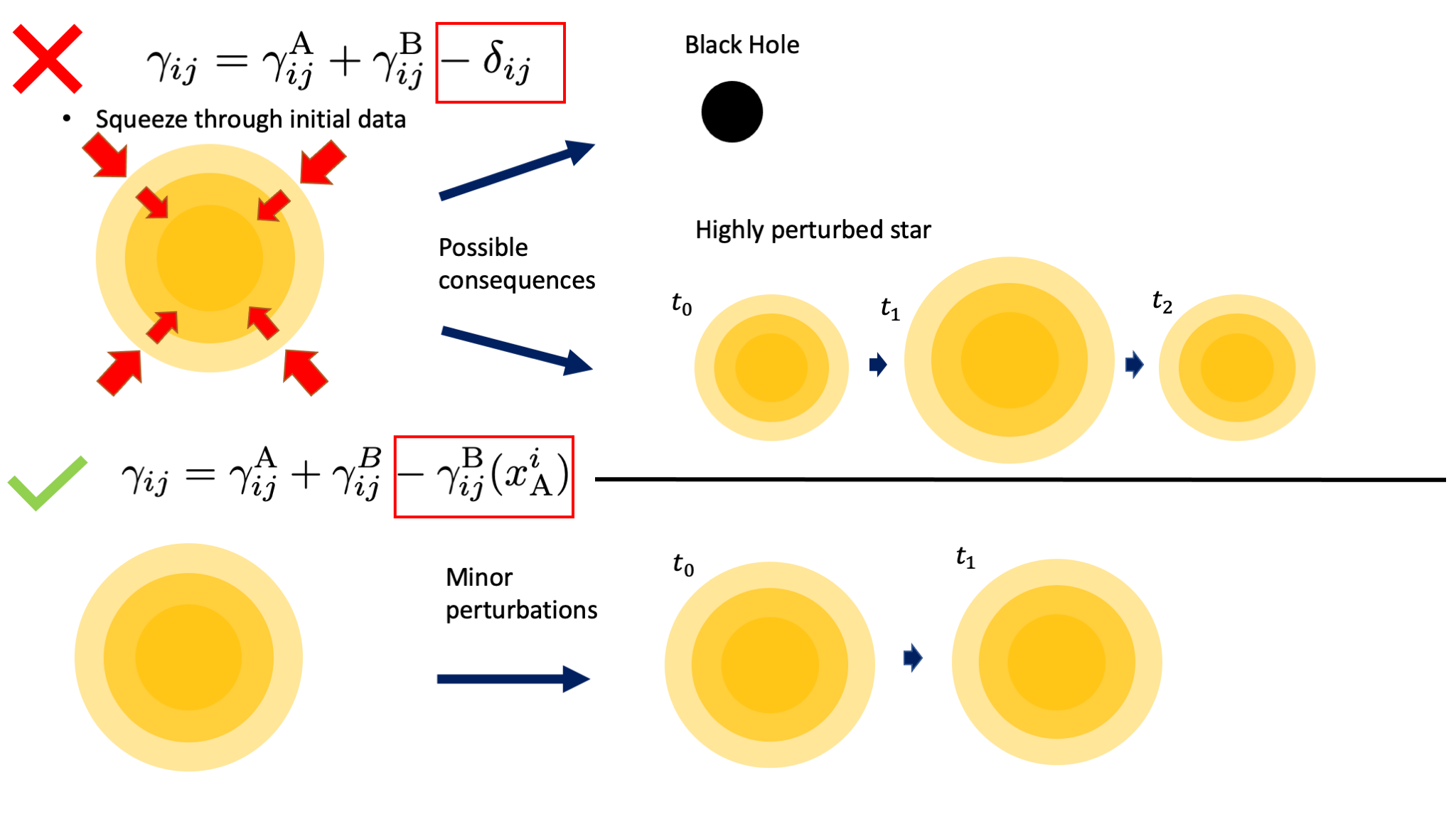
Figure 2: Graphical illustration of the spurious dynamics that may be introduced by the simple superposition procedure (43). Upper panel: The spurious increase in the volume element mimics a squeezing of the stellar core that effects a pulsation of the star or may even trigger gravitational collapse to a BH. Lower panel: No such squeezing occurs with the adjusted superposition (45), and the binary evolution starts with approximately unperturbed stars.

Fig. 2 together with some of the possible consequences. As we will see, this qualitative interpretation is fully borne out by the phenomenology we observe in the binaries’ time evolutions.

Finally, we would like to emphasise that, while evaluating the constraint violations is in general a good rule of thumb to check whether the field configuration is a solution of the system, it does not inform one whether it is the intended solution; a system with some constraint violation may have drifted closer to a different, unintended solution. In the present case, in addition to the increased constraint violation, the constructed BS solutions possess significant excitations. Thus, while applying a constraint damping system like conformal Z4 [92, 93] may eventually drive the system to a solution, it may no longer be what was originally intended to be the initial condition of an unexcited BS star.

3.2 Improved superposition

The problem of the simple superposition is encapsulated by Eq. (44) and the resulting deviation of the volume elements at the stars’ centres away from their equilibrium values. At the same time, the equation presents us with a concrete recipe to mitigate this error: we merely need to replace in the simple superposition (43) the first relation $\gamma_{ij}=\gamma_{ij}^{\rm A}+\gamma_{ij}^{B}-\delta_{ij}$ by

$$\boxed{\gamma_{ij}=\gamma_{ij}^{\rm A}+\gamma_{ij}^{\rm B}-\gamma_{ij}^{\rm B}(x^{i}_{\rm A})=\gamma_{ij}^{\rm A}+\gamma_{ij}^{\rm B}-\gamma_{ij}^{\rm A}(x^{i}_{\rm B})\,.}$$ (45)

The two expressions on the right-hand side are indeed equal thanks to the symmetry of our binary: its constituents have equal mass, no spin and their velocity components satisfy $v_{\rm A}^{i}v_{\rm A}^{j}=v_{\rm B}^{i}v_{\rm B}^{j}$ for all $i,\,j=1,\,2,\,3$ in the centre-of-mass frame. Equation (45) manifestly ensures that at positions $x_{\rm A}^{i}$ and $x_{\rm B}^{i}$ we now recover the respective star’s equilibrium metric and, hence, volume element. We graphically illustrate this improvement in the bottom panel of Fig. 2.

A minor complication arises from the fact that the resulting spatial metric does not asymptote towards $\delta_{ij}$ as $R\rightarrow\infty$. We accordingly impose outgoing Sommerfeld boundary conditions on the asymptotic background metric $2\delta_{ij}-\gamma_{ij}^{\rm A}(x^{i}_{\rm B})$; in a set of test runs, however, we find this correction to result in very small changes well below the simulation’s discretisation errors.

Finally, we note that the leading-order correction to the superposition as written in Eq. (45) does not work for asymmetric configurations with unequal masses or spins. Generalising the method to arbitrary binaries requires the subtraction of a spatially varying term rather than a constant $\gamma_{ij}^{\rm B}(x^{i}_{\rm A})=\gamma_{ij}^{\rm A}(x^{i}_{\rm B})$ or $\delta_{ij}$. Such a generalisation may consist, for example, of a weighted sum of the terms $\gamma_{ij}^{\rm A}(x^{i}_{\rm B})$ and $\gamma_{ij}^{\rm B}(x^{i}_{\rm A})$. Leaving this generalisation for future work, we will focus on equal-mass systems in the remainder of this study and explore the degree of improvement achieved with Eq. (45).

4 Models and results

For our analysis of the two types of superposed initial data, we will now discuss time evolutions of binary BS head-on collisions. A head-on collision is characterised by the two individual BS models and three further parameters, the initial separation in units of the ADM mass, $d/M$, and the initial velocities $v_{\rm A}$ and $v_{\rm B}$ of the BSs. We perform all our simulations in the centre-of-mass frame, so that for equal-mass binaries, $v_{\rm A}=-v_{\rm B}=\mathrel{\vbox{\hbox{\scriptsize.}\hbox{\scriptsize.}}}v$. One additional parameter arises from the type of superposition used for the initial data construction: we either use the “plain” superposition of Eq. (43) or the “adjusted” method (45).

For all our simulations, we set $v=0.1$; this value allows us to cover a wide range of initial separations without the simulations becoming prohibitively long.

Table 2: The four types of BS binary head-on collisions simulated in this study. The individual BSs A and B are given either by the mini or solitonic model of Table 1, and start with initial velocity $v$ directed towards each other. The initial data is constructed either by plain superposition (43) or by adjusting the superposed data according to Eq. (45). For each type of binary, we perform five collisions with initial separations $d$ listed in the final column.

Label	star A	star B	$v$	initial data	$d/M$
mini	mini	mini	$0.1$	plain	75.5, 101, 126, 151, 176
+mini	mini	mini	$0.1$	adjusted	75.5, 101, 126, 151, 176
soli	soli	soli	$0.1$	plain	16.7, 22.3, 27.9, 33.5, 39.1
+soli	soli	soli	$0.1$	adjusted	16.7, 22.3, 27.9, 33.5, 39.1

The BS binary configurations summarised in Table 2 then result in four sequences of head-on collisions labelled mini, +mini, soli and +soli, depending in the nature of the constituent BSs and the superposition method. For each sequence, we vary the BSs initial separation $d$ to estimate the dependence of the outcome on $d$. First, however, we test our interpretation of the improved superposition (45) by computing the level of constraint violations in the initial data.

4.1 Initial constraint violations

As discussed in Sec. 3.1 and in Appendix A of Ref. [1], the main shortcoming of the plain superposition procedure consists in the distortion of the volume element near the individual BSs’ centres and the resulting perturbation of the mass-energy inside the stars away from their equilibrium values. If this interpretation is correct, we would expect this effect to manifest itself in an elevated level of violation of the Hamiltonian constraint (19) which relates the energy density to the spacetime curvature. Put the other way round, we would expect our improved method (45) to reduce the Hamiltonian constraint violation. This is indeed the case as demonstrated in the upper panels of Fig. 3 where we plot the Hamiltonian constraint violation of the initial data along the collision axis for the configurations mini and +mini with $d=101\,M$ and the configurations soli and +soli with $d=22.3\,M$.

Figure 3: Upper row: The Hamiltonian constraint violation $\mathcal{H}$ – Eq. (19) – normalised by the respective BS’s central energy density $16\pi\rho_{\rm ctr}$ is plotted along the collision axis of the binary configurations mini, +mini with $d=101\,M$ (left) and soli, +soli with $d=22.3\,M$ (right). The degree of violations is substantially reduced in the BS interior by using the improved superposition (45) for +mini and +soli relative to their plain counterparts; the maxima of $\mathcal{H}$ have dropped by over an order of magnitude in both cases. Bottom row: The same analysis for the momentum constraint $\mathcal{M}_{x}$ normalised by the central BS’s momentum density $8\pi j_{x}$. Here the improvement is less dramatic, but still yields a reduction by a factor of a few in the BS core.

In the limit of zero boost velocity $v=0$, this effect is even tractable through an analytic calculation which confirms that the improved superposition (45) ensures $\mathcal{H}=0$ at the BS’s centres in isotropic coordinate; see A for more details.

Our adjustment (45) also leads to a reduction of the momentum constraint violations of the initial data, although the effect is less dramatic here. The bottom panels of Fig. 3 display the momentum constraint $\mathcal{M}_{x}$ of Eq. (20) along the collision axis normalised by the momentum density $8\pi j_{x}$; we see a reduction by a factor of a few over large parts of the BS interior for the modified data +mini and +soli.

The overall degree of initial constraint violations is rather small in all cases, well below $0.1\,\%$ for our adjusted data. These data should therefore also provide a significantly improved initial guess for a full constraint solving procedure. We leave such an analysis for future work and in the remainder of the work explore the impact of the adjustment (45) on the physical results obtained from the initial data’s time evolutions.

4.2 Convergence and numerical uncertainties

In order to put any differences in the time evolutions into context, we need to understand the uncertainties inherent to our numerical simulations. For this purpose, we have studied the convergence of the GW radiation generated by the head-on collisions of mini and solitonic BSs.

Figure 4 displays the convergence of the radiated energy $E_{\rm rad}$ as a function of time for the +mini configuration with $d=101\,M$ of Table 1 obtained for grid resolutions $h_{1}=M/6.35$, $h_{2}=M/9.53$ and $h_{3}=M/12.70$ on the innermost refinement level and corresponding grid spacings on the other levels. The functions $E_{\rm rad}(t)$ and their differences are shown in the bottom and top panel, respectively, of Fig. 4 together with an amplification of the high-resolution differences by the factor $Q_{2}=2.86$ for second-order convergence. The observation of second-order convergence is compatible with the second-order ingredients of the Lean code, prolongation in time and the outgoing radiation boundary conditions. We believe that this dominance is mainly due to the smooth behaviour of the BS centre as compared with the case of black holes [94]. By using the second-order Richardson extrapolated result, we determine the discretisation error of our energy estimates as $0.9\,\%$ for $h_{3}$ which is the resolution employed for all remaining mini BS collisions. We have performed the same convergence analysis for the plain-superposition counterpart mini and for the dominant $(\ell,m)=(2,0)$ multipole of the Newman-Penrose scalar of both configurations and obtained the same convergence and very similar relative errors.

In Fig. 5, we show the same convergence analysis for the solitonic collision +soli with $d=22.3\,M$ and resolutions $h_{1}=M/22.9$, $h_{2}=M/45.9$, $h_{3}=M/68.8$. We observe second-order convergence during merger and ringdown and slightly higher convergence in the earlier infall phase.

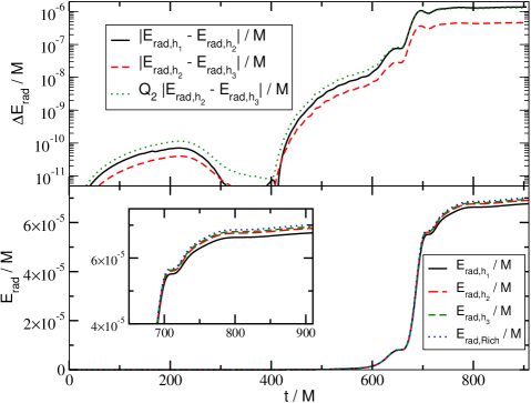
Figure 4: Convergence analysis for the GW energy extracted at $R_{\rm ex}=252\,M$ from the head-on collision +mini of Table 1 with $d=101\,M$. For the resolutions $h_{1}=M/6.35$, $h_{2}=M/9.53$ and $h_{3}=12.70$ (on the innermost refinement level), we obtain convergence close to second order (upper panel). The numerical error, obtained by comparing our results with the second-order Richardson extrapolated values (bottom panel), is $0.9\,\%$ ($1.6\,\%$, $3.6\,\%$) for our high (medium, coarse) resolutions.

Figure 5: Convergence analysis as in Fig. 4 but for the configuration +soli of Table 1 with $d=22.3\,M$ and resolutions $h_{1}=M/22.9$, $h_{2}=M/45.9$ and $h_{3}=M/68.8$. The numerical error, obtained by comparing our results with the second-order Richardson extrapolated values (bottom panel), is $0.03\,\%$ ($0.07\,\%$, $0.6\,\%$) for our high (medium, coarse) resolutions.

For the uncertainty estimate we conservatively use the second-order Richardson extrapolated result and obtain a discretisation error of about $0.07\,\%$ for our medium resolution $h_{2}$ which is the value we employ in our solitonic production runs. Again, we have repeated this analysis for the plain soli counterpart and the $(2,0)$ GW multipole observing the same order of convergence and similar uncertainties. Our error estimate for the solitonic configurations is rather small in comparison to the mini BS collisions and we cannot entirely rule out a fortuitous cancellation of errors in our simulations. From this point on, we therefore use a conservative discretisation error estimate of $1\,\%$ for all our BS simulations.

A second source of uncertainty in our results is due to the extraction of the GW signal at finite radii rather than $\mathcal{I}^{+}$. We determine this error by extracting the signal at multiple radii, fitting the resulting data by the series expansion $f=f_{0}+f_{1}/r$, and comparing the result at our outermost extraction radius with the limit $f_{0}$. This procedure results in errors in $E_{\rm rad}$ ranging between $0.5\,\%$ and $3\,\%$. With the upper range, we arrive at a conservative total error budget for discretisation and extraction of about $4\,\%$. As a final test, we have repeated the mini and +mini collisions for $d=101\,M$ with the independent GRChombo code [95, 96] using the CCZ4 formulation [93] and obtain the same results within $\approx 1.5\,\%$. Bearing in mind these tests and a $4\,\%$ error budget, we next study the dynamics of the BS head-on collisions with and without our adjustment of the initial data.

4.3 Radiated gravitational-wave energy

For our first test, we compute the total radiated GW energy for all our head-on collisions focusing in particular on its dependence on the initial separation $d$ of the BS centres. In this estimate we exclude any spurious or “junk” radiation content of the initial data by starting the integration at $t=R_{\rm ex}+40\,M$. Unless specified otherwise, all our results are extracted at $R_{\rm ex}=300\,M$ for mini BS collisions and $R_{\rm ex}=84\,M$ for the solitonic binaries.

Figure 6: The GW energy $E_{\rm rad}$ generated in the head-on collision of mini (upper panel) and solitonic (lower panel) BS binaries starting with initial separation $d$ and velocity $v=0.1$ towards each other. For comparison, a non-spinning, equal-mass BH binary colliding head-on with the same boost velocity $v=0.1$ radiates $E_{\rm rad}=6.0\times 10^{-4}\,M$ [89].

The main effect of increasing the initial separation is a reduction of the (negative) binding energy of the binary and a corresponding increase of the collision velocity around merger. In the large $d$ limit, however, this effect becomes negligible. For the comparatively large initial separations chosen in our collisions, we would therefore expect the function $E_{\rm rad}$ to be approximately constant, possibly showing a mild increase with $d$. The mini BS collisions shown as black $\times$ symbols in the upper panel of Fig. 6 exhibit a rather different behaviour: the radiated energy rapidly decreases with $d$ and only levels off for $d\gtrsim 150\,M$. We have verified that the excess energy for smaller $d$ is not due to an elevated level of junk radiation which consistently contribute well below $0.1\,\%$ of $E_{\rm rad}$ in all our mini BS collisions and has been excluded from the results of Fig. 6 anyway. The +mini BS collisions, in contrast, results in an approximately constant $E_{\rm rad}$ with a total variation approximately at the level of the numerical uncertainties. For $d\gtrsim 150\,M$, both types of initial data yield compatible results, as is expected. The key benefit of our adjusted initial data is that they provide reliable results even for smaller initial separations suitable for starting BS inspirals.

The discrepancy is less pronounced for the head-on collisions of solitonic BS collisions; both types of initial data result in approximately constant $E_{\rm rad}$. They differ, however, in the predicted amount of radiation at a level that is significant compared to the numerical uncertainties. As we will see below, this difference is accompanied by drastic differences in the BS’s dynamics during the long infall period. We furthermore note that the mild but steady increase obtained for the adjusted +soli agrees better with the physical expectations.

The differences in the total radiated GW energy also manifest themselves in different amplitudes of the $(2,0)$ multipole of the Newman-Penrose scalar $\Psi_{4}$. This is displayed in Figs. 7 and 8 where we show the GW modes for the mini and solitonic collisions, respectively. The most prominent difference between the results for plain and adjusted initial data is the significant variation of the amplitude of the $(2,0)$ mode in the plain mini BS collisions in the upper panel of Fig. 7. In contrast, the differences in the amplitudes in Fig. 8 for the solitonic collisions are very small. In fact, the differences in the radiated energy of the soli and +soli collisions mostly arise from a minor stretching of the signal for the soli case; this effect is barely perceptible in Fig. 8 but is amplified by the integration in time when we calculate the energy. Finally, we note the different times of arrival of the main pulses in Fig. 8; especially for larger initial separation, the merger occurs earlier for the soli configurations than for their adjusted counterparts +soli. We will discuss this effect together with the evolution of the scalar field amplitude in the next subsection.

Figure 7: The $(2,0)$ mode of the Newman-Penrose scalar for the mini boson star collisions of Table 1.

Figure 8: The $(2,0)$ mode of the Newman-Penrose scalar for the solitonic boson star collisions of Table 1.

4.4 Evolution of the scalar amplitude and gravitational collapse

The adjustment (45) in the superposition of oscillatons was originally developed in Ref. [1] to reduce spurious modulations in the scalar field amplitude; cf. their Fig. 7. In our simulations, this effect manifests itself most dramatically in the collisions of our solitonic BS configurations soli and +soli. From Fig. 1, we recall that the single-BS constituents of these binaries are stable, but highly compact stars, located fairly close to the instability threshold. We would therefore expect them to be more sensitive to spurious modulations in their central energy density. This is exactly what we observe in all time evolutions of the soli configurations starting with plain-superposition initial data. As one example, we show in Fig. 9 the scalar amplitude at the individual BS centres and the BS trajectories as functions of time for the soli and +soli configurations starting with initial separation $d=22.3\,M$.

Figure 9: The central scalar-field amplitude $|\varphi_{\rm ctr}|$ as a function of time for one BS in the head-on collisions of solitonic BSs with distance $d=22.3\,M$ (black solid and red long-dashed) as well as a single BS spacetime with the same parameters (green dashed) and the same single BS spacetime “poisoned” with the metric perturbation (44) that would arise in a simple superposition (see text for details). The dotted vertical lines mark the first location of an apparent horizon in the simulation of the same colour; as expected, no horizon ever forms in the evolution of the unpoisoned single BS. In the bottom panel, we show for reference the coordinate trajectories of the BS centres as obtained from locally Gauss-fitting the scalar profile. Around merger this procedure becomes inaccurate, so that the values around $t\approx 70\,M$ should be regarded as qualitative measures, only.

Let us first consider the soli configuration using plain superposition displayed by the solid (black) curves. In the upper panel of Fig. 9, we clearly see that the scalar amplitude steadily increases, reaching a maximum around $t\approx 30\,M$ and then rapidly drops to a near-zero level. Our interpretation of this behaviour as a collapse to a BH is confirmed by the horizon finder which reports an apparent horizon of irreducible mass $m_{\rm irr}=0.5\,M$ just before the scalar field amplitude collapses; the time of the first identification of an apparent horizon is marked by the vertical dotted black line at $t\approx 30\,M$. For reference we plot in the bottom panel the trajectory of the BS centres along their collision (here the $x$) axis. In agreement with the horizon mass $m_{\rm irr}=0.5\,M$, the trajectory clearly indicates that around $t\approx 30\,M$, the BSs are still far away from merging into a single BH; in units of the ADM mass, the individual BS radius is $r_{99}=2.78\,M$. We interpret this early BH collapse as a spurious feature due to the use of plain superposition in the initial data construction. This behaviour is also seen in the case of the real scalar field oscillatons in [1].

We have tested this hypothesis with the evolution of the adjusted initial data. These exhibit a drastically different behaviour in the collision +soli displayed by the dashed (red) curves in Fig. 9. Throughout most of the infall, the central scalar amplitude is constant, it increases mildly when the BS trajectories meet near $x=0$, and then rapidly drops to zero. Just as the maximum amplitude is reached, the horizon finder first computes an apparent horizon, now with $m_{\rm irr}=0.99\,M$, as expected for a BH resulting from the merger; see the vertical red line in the figure.

As a final test of our interpretation, we compare the behaviour of the binary constituents with that of single BSs boosted with the same velocity $v=0.1$. As expected, the scalar field amplitude at the centre of such a single BS remains constant within high precision, about $\mathcal{O}(10^{-5})$, on the timescale of our collisions. We have then repeated the single BS evolution by poisoning the initial data with the very same term (44) that is also added near a single BS’s centre by the plain-superposition procedure. The resulting scalar amplitude at the centre of this poisoned BS is shown as the dash-dotted (blue) curve in Fig. 9 and nearly overlaps with the corresponding curve of the soli binary. Furthermore, the poisoned single BS collapses into a BH after nearly the same amount of time as indicated by the vertical blue dotted curve in the figure. Clearly this behaviour of the single boosted BS is unphysical, and strongly indicates that the plain superposition of initial data introduces the same unphysical behaviour to our soli binary constituents. We have repeated this analysis for our entire sequence of soli binaries with very similar results: the individual BSs always collapse to distinct BHs about $\Delta t\approx 50\,M$ before the binary merger.

Finally, the trajectories in the bottom panel of Fig. 9 indicate that the BS merger occurs a bit later for the +soli case than its plain-superposition counterpart soli. This is indeed a systematic effect we see for all initial separations $d$ and which agrees with the different arrival times of the peak GW signals that we have already noticed in Fig. 8. We do not have a rigorous explanation of this effect, but note that the two trajectories in Fig. 9 start diverging right at the time of spurious BH formation in the soli binary. Perhaps some of the binding energy in BS collisions is converted into deformation energy rather than simply kinetic energy of the stars’ centres of mass, slowing down the infall compared to the BH case. Another explanation may consider the generally repulsive character of the scalar field which endows it with support against gravitational collapse. When the infalling BSs collapse to BHs, the scalar field essentially disappears as a potentially repulsive ingredient and the ensuing collision is sped up. Whatever ultimately generates this effect, the key observation of our study is that even rather mild imperfections in the initial data can drastically affect the physical outcome of the time evolution.

5 Conclusions

We have simulated head-on collisions of equal-mass, non-spinning boson stars and the GW radiation generated in the process. The main focus of our study is the construction of BS binary initial data and the ensuing impact of systematic errors on the physical results of the simulations. In particular, we have contrasted the relatively common method of plain superposition according to Eq. (43) with the adjusted procedure (45) first identified in Ref. [1] for oscillatons.

Our results demonstrate that the adjustment (45) in the construction of initial data leads to major improvements in the initial constraint violations and the time evolutions of binary BS collisions. In contrast, we find that the use of plain superposition for BS binary initial data may not only result in quantitatively wrong physical diagnostics but can even result in completely spurious physical behaviour such as premature gravitational collapse. In spite of the great simplicity of the adjustment (45) and its success in overcoming the most severe errors in the ensuing evolution, it is not free of shortcomings. (i) In its present form, the adjustment only works for a restricted class of binaries, namely equal-mass systems with no spin and velocity vectors satisfying $v_{\rm A}^{i}v_{\rm A}^{j}=v_{\rm B}^{i}v_{\rm B}^{j}$. (ii) Even with the adjustment, the initial data contain some residual constraint violations; it should therefore primarily be regarded as an improved initial guess for a constraint solving procedure rather than the “real deal” in its own right. These shortcomings clearly point towards the most urgent generalisations of our work, overcoming the symmetry restrictions and adding a numerical constraint solver.

References

Appendix A Analytic treatment of the Hamiltonian constraint

For the case of two non-boosted BSs, we can analytically compute the Hamiltonian constraint violation at the stars’ centres. Let us consider for this purpose the metric ansatz (31). From this line element, we directly extract the spatial metric

$$\gamma_{ij}^{A}=\psi_{\rm A}^{4}\delta_{ij}\,.$$ (46)

for a non-boosted BS at position $x_{\rm A}^{i}$. This metric is time-independent, so that for zero shift vector the extrinsic curvature vanishes, $K_{ij}^{\rm A}=0$. For the second binary member, we likewise obtain a metric $\gamma^{\rm B}_{ij}$ and extrinsic curvature $K^{\rm B}_{ij}=0$, now centred at position $x_{\rm B}^{i}$.

For sufficiently large initial separation $d=||x_{\rm B}^{i}-x_{\rm A}^{i}||$, the exponential falloff of the scalar field implies

$$\phi_{\rm A}(x_{\rm B}) =\phi_{\rm B}(x_{\rm A})\approx 0\,,$$ (47)

$$\Pi_{\rm A}(x_{\rm B}) =\Pi_{\rm B}(x_{\rm A})\approx 0\,.$$

The superposition of the two stars’ scalar fields results in

$$\varphi=\varphi_{\rm A}+\varphi_{\rm B}\,,\hskip 24.18501pt~{}~{}~{}~{}~{}~{}~{}~{}~{}~{}\Pi=\Pi_{\rm A}+\Pi_{\rm B}\,,$$ (48)

and, combined with Eqs. (47),

$$\rho(x_{\rm A}) =\rho_{A}(x_{\rm A})\,,$$ (49)

$$\rho(x_{\rm B}) =\rho_{B}(x_{\rm B})\,.$$

The single BS spacetimes are solutions to the Einstein equations; by using Eq. (46), their individual Hamiltonian constraints (19) simplify to

$$\mathcal{H}_{\rm A}=8\delta^{ij}\partial_{i}\partial_{j}\psi_{\rm A}+16\pi\psi_{\rm A}^{5}\rho_{\rm A}=0\,,$$ (50)

and likewise for star B.

Next, we construct a binary spacetime by superposing the metric which leads to

$$\psi^{4}=\psi_{\rm A}^{4}+\psi_{\rm B}^{4}-c^{4}\,,$$ (51)

where $c$ is a constant which we keep arbitrary for the moment. For the Hamiltonian constraint of the superposed spacetime at the centre of star A, we find

$$\mathcal{H}(x_{\rm A}^{i}) =8\delta^{ij}\partial_{i}\partial_{j}{\psi_{\rm A}({x_{\rm A}^{i}})}+8\delta^{ij}\partial_{i}\partial_{j}{\psi_{\rm B}({x_{\rm A}^{i}})}$$ (52)

$$+16\pi\left[{\psi_{A}({x_{\rm A}^{i}})}^{4}+{\psi_{\rm B}({x_{\rm A}^{i}})}^{4}-c^{4}\right]^{5/4}\rho(x_{\rm A}^{i})\,.$$

We can now choose the constant $c$ in accordance with the “trick” in Eq. (45), namely

$$c=\psi_{B}(x_{A}^{i})\,,$$ (53)

and the constraint simplifies to

$$\mathcal{H}(x_{\rm A}^{i}) =8\delta^{ij}\partial_{i}\partial_{j}{\psi_{\rm A}({x_{\rm A}^{i}})}+8\delta^{ij}\partial_{i}\partial_{j}{\psi_{\rm B}({x_{\rm A}^{i}})}$$ (54)

$$+16\pi{\psi_{\rm A}({x_{\rm A}^{i}})}^{4}\rho(x_{\rm A}^{i})\,.$$

By Eq. (50), the derivative of the conformal factor $\psi_{\rm A}$ cancels out the density $\rho_{\rm A}$, so that

$$\mathcal{H}(x_{\rm A}^{i}) =8\delta^{ij}\partial_{i}\partial_{j}{\psi_{\rm B}({x_{\rm A}^{i}})}\,.$$ (55)

Using the analogue of Eq. (50) for star B, we trade the right-hand side for the energy density,

$$\mathcal{H}(x_{\rm A}^{i}) =-16\pi{\psi_{\rm B}({x_{\rm A}^{i}})}^{4}\rho_{\rm B}(x_{\rm A}^{i})\,.$$ (56)

For sufficiently large separation $d$ of the stars, however, this vanishes by Eq. (47) which is the result we wished to compute. By symmetry, we likewise obtain $\mathcal{H}(x_{\rm B}^{i})=0$, which concludes our calculation.

References

- [1] T. Helfer, E. A. Lim, M. A. G. Garcia, and M. A. Amin. Gravitational Wave Emission from Collisions of Compact Scalar Solitons. Phys. Rev. D, 99(4):044046, 2019.
- [2] B. P. Abbott et al. Observation of Gravitational Waves from a Binary Black Hole Merger. Phys. Rev. Lett., 116(6):061102, 2016.
- [3] B. P. Abbott et al. GWTC-1: A Gravitational-Wave Transient Catalog of Compact Binary Mergers Observed by LIGO and Virgo during the First and Second Observing Runs. Phys. Rev. X, 9(3):031040, 2019.
- [4] R. Abbott et al. GWTC-2: Compact Binary Coalescences Observed by LIGO and Virgo During the First Half of the Third Observing Run. Phys. Rev. X, 11:021053, 2021.
- [5] Emanuele Berti et al. Testing General Relativity with Present and Future Astrophysical Observations. Class. Quant. Grav., 32:243001, 2015.
- [6] B. P. Abbott et al. Tests of general relativity with GW150914. Phys. Rev. Lett., 116(22):221101, 2016.
- [7] B.P. Abbott et al. Tests of General Relativity with GW170817. Phys. Rev. Lett., 123(1):011102, 2019.
- [8] B.P. Abbott et al. Tests of General Relativity with the Binary Black Hole Signals from the LIGO-Virgo Catalog GWTC-1. Phys. Rev. D, 100(10):104036, 2019.
- [9] R. Abbott et al. Tests of general relativity with binary black holes from the second LIGO-Virgo gravitational-wave transient catalog. Phys. Rev. D, 103(12):122002, 2021.
- [10] C. J. Moore, E. Finch, R. Buscicchio, and D. Gerosa. Testing general relativity with gravitational-wave catalogs: the insidious nature of waveform systematics. 3 2021.
- [11] D. Trifirò, R. O’Shaughnessy, D. Gerosa, E. Berti, M. Kesden, T. Littenberg, and U. Sperhake. Distinguishing black-hole spin-orbit resonances by their gravitational wave signatures. II: Full parameter estimation. Phys. Rev. D, 93(4):044071, 2016. arXiv:1507.05587 [gr-qc].
- [12] K. Belczynski et al. Evolutionary roads leading to low effective spins, high black hole masses, and O1/O2 rates for LIGO/Virgo binary black holes. Astron. Astrophys., 636:A104, 2020.
- [13] R. Abbott et al. Population Properties of Compact Objects from the Second LIGO-Virgo Gravitational-Wave Transient Catalog. Astrophys. J. Lett., 913(1):L7, 2021.
- [14] Vishal Baibhav, Davide Gerosa, Emanuele Berti, Kaze W. K. Wong, Thomas Helfer, and Matthew Mould. The mass gap, the spin gap, and the origin of merging binary black holes. Phys. Rev. D, 102(4):043002, 2020.
- [15] Davide Gerosa and Maya Fishbach. Hierarchical mergers of stellar-mass black holes and their gravitational-wave signatures. 5 2021.
- [16] B. P. Abbott et al. A gravitational-wave standard siren measurement of the Hubble constant. Nature, 551(7678):85–88, 2017.
- [17] B. P. Abbott et al. A Gravitational-wave Measurement of the Hubble Constant Following the Second Observing Run of Advanced LIGO and Virgo. Astrophys. J., 909(2):218, 2021.
- [18] L. Barack et al. Black holes, gravitational waves and fundamental physics: a roadmap. Class. Quant. Grav., 36(14):143001, 2019.
- [19] B. P. Abbott et al. GW170817: Observation of Gravitational Waves from a Binary Neutron S+tar Inspiral. Phys. Rev. Lett., 119(16):161101, 2017.
- [20] B. P. Abbott et al. Gravitational Waves and Gamma-rays from a Binary Neutron Star Merger: GW170817 and GRB 170817A. Astrophys. J., 848(2):L13, 2017.
- [21] V. Cardoso, L. Gualtieri, C. Herdeiro, and U. Sperhake. Exploring New Physics Frontiers Through Numerical Relativity. Living Rev. Relativity, 18:1, 2015. arXiv:1409.0014 [gr-qc].
- [22] Richard Brito, Vitor Cardoso, and Paolo Pani. Superradiance. Lect. Notes Phys., 906:pp.1–237, 2015.
- [23] J. A. Wheeler. Geons. Phys. Rev., 97:511–536, 1955.
- [24] Thomas W. Baumgarte and Stuart L. Shapiro. Numerical Relativity: Starting from Scratch. Cambridge University Press, 2 2021.
- [25] David A. Feinblum and William A. McKinley. Stable States of a Scalar Particle in Its Own Gravational Field. Phys. Rev., 168(5):1445, 1968.
- [26] David J. Kaup. Klein-Gordon Geon. Phys. Rev., 172:1331–1342, 1968.
- [27] Remo Ruffini and Silvano Bonazzola. Systems of selfgravitating particles in general relativity and the concept of an equation of state. Phys. Rev., 187:1767–1783, 1969.
- [28] R. Brito, V. Cardoso, C. A. R. Herdeiro, and E. Radu. Proca stars: Gravitating Bose–Einstein condensates of massive spin 1 particles. Phys. Lett., B752:291–295, 2016.
- [29] M. Alcubierre, J. Barranco, A. Bernal, J. C. Degollado, A. Diez-Tejedor, M. Megevand, D. Nunez, and O. Sarbach. -Boson stars. Class. Quant. Grav., 35(19):19LT01, 2018.
- [30] M. Choptuik, R. Masachs, and B. Way. Multioscillating Boson Stars. Phys. Rev. Lett., 123(13):131101, 2019.
- [31] F. Pretorius. Evolution of Binary Black-Hole Spacetimes. Phys. Rev. Lett., 95:121101, 2005. gr-qc/0507014.
- [32] M. Campanelli, C. O. Lousto, P. Marronetti, and Y. Zlochower. Accurate Evolutions of Orbiting Black-Hole Binaries without Excision. Phys. Rev. Lett., 96:111101, 2006. gr-qc/0511048.
- [33] J. G. Baker, J. Centrella, D.-I. Choi, M. Koppitz, and J. van Meter. Gravitational-Wave Extraction from an inspiraling Configuration of Merging Black Holes. Phys. Rev. Lett., 96:111102, 2006. gr-qc/0511103.
- [34] U. Sperhake. The numerical relativity breakthrough for binary black holes. Class. Quant. Grav., 32(12):124011, 2015.
- [35] R. C. Tolman. Static Solutions of Einstein’s Field Equations for Spheres of Fluid. Phys. Rev., 55:364–373, 1939.
- [36] J. R. Oppenheimer and G. M. Volkoff. On Massive Neutron Cores. Phys. Rev., 55:374–381, 1939.
- [37] J. D. Breit, S. Gupta, and A. Zaks. Cold Bose Stars. Phys. Lett. B, 140:329–332, 1984.
- [38] Marcelo Gleiser and Richard Watkins. Gravitational Stability of Scalar Matter. Nucl. Phys. B, 319:733–746, 1989.
- [39] Edward Seidel and Wai-Mo Suen. Dynamical Evolution of Boson Stars. 1. Perturbing the Ground State. Phys. Rev. D, 42:384–403, 1990.
- [40] T. D. Lee and Y. Pang. Nontopological solitons. Phys. Rept., 221:251–350, 1992.
- [41] Philippe Jetzer. Boson stars. Phys. Rept., 220:163–227, 1992.
- [42] Andrew R. Liddle and Mark S. Madsen. The Structure and formation of boson stars. Int. J. Mod. Phys. D, 1:101–144, 1992.
- [43] J. Balakrishna, E. Seidel, and W.-M. Suen. Dynamical evolution of boson stars. 2. Excited states and selfinteracting fields. Phys. Rev. D, 58:104004, 1998.
- [44] M. Colpi, S. L. Shapiro, and I. Wasserman. Boson Stars: Gravitational Equilibria of Selfinteracting Scalar Fields. Phys. Rev. Lett., 57:2485–2488, 1986.
- [45] T. D. Lee. Soliton Stars and the Critical Masses of Black Holes. Phys. Rev. D, 35:3637, 1987.
- [46] Franz E. Schunck and Diego F. Torres. Boson stars with generic selfinteractions. Int. J. Mod. Phys. D, 9:601–618, 2000.
- [47] Betti Hartmann, Burkhard Kleihaus, Jutta Kunz, and Isabell Schaffer. Compact Boson Stars. Phys. Lett. B, 714:120–126, 2012.
- [48] J. C. Bustillo, N. Sanchis-Gual, A. Torres-Forné, J. A. Font, A. Vajpeyi, R. Smith, C. Herdeiro, E. Radu, and S. H. W. Leong. GW190521 as a Merger of Proca Stars: A Potential New Vector Boson of+ eV. Phys. Rev. Lett., 126(8):081101, 2021.
- [49] N. Sennett, T. Hinderer, J. Steinhoff, A. Buonanno, and S. Ossokine. Distinguishing Boson Stars from Black Holes and Neutron Stars from Tidal Interactions in Inspiraling Binary Systems. Phys. Rev. D, 96(2):024002, 2017.
- [50] F. Di Giovanni, N. Sanchis-Gual, P. Cerdá-Durán, M. Zilhão, C. Herdeiro, J. A. Font, and E. Radu. Dynamical bar-mode instability in spinning bosonic stars. Phys. Rev. D, 102(12):124009, 2020.
- [51] Alexandre Toubiana, Stanislav Babak, Enrico Barausse, and Luis Lehner. Modeling gravitational waves from exotic compact objects. Phys. Rev. D, 103(6):064042, 2021.
- [52] Y. Kobayashi, M. Kasai, and T. Futamase. Does a boson star rotate? Phys. Rev. D, 50:7721–7724, 1994.
- [53] F. E. Schunck and E. W. Mielke. Rotating boson star as an effective mass torus in general relativity. Phys. Lett., A249:389–394, 1998.
- [54] Fintan D. Ryan. Spinning boson stars with large selfinteraction. Phys. Rev. D, 55:6081–6091, 1997.
- [55] Shijun Yoshida and Yoshiharu Eriguchi. Nonaxisymmetric boson stars in Newtonian gravity. Phys. Rev. D, 56:6370–6377, 1997.
- [56] Shijun Yoshida and Yoshiharu Eriguchi. Rotating boson stars in general relativity. Phys. Rev. D, 56:762–771, 1997.
- [57] Shijun Yoshida and Yoshiharu Eriguchi. New static axisymmetric and nonvacuum solutions in general relativity: Equilibrium solutions of boson stars. Phys. Rev. D, 55:1994–2001, 1997.
- [58] F. E. Schunck and E. W. Mielke. Boson stars: Rotation, formation, and evolution. Gen. Rel. Grav., 31:787, 1999.
- [59] Burkhard Kleihaus, Jutta Kunz, and Meike List. Rotating boson stars and Q-balls. Phys. Rev. D, 72:064002, 2005.
- [60] B. Kleihaus, J. Kunz, M. List, and I. Schaffer. Rotating Boson Stars and Q-Balls. II. Negative Parity and Ergoregions. Phys. Rev. D, 77:064025, 2008.
- [61] Burkhard Kleihaus, Jutta Kunz, and Stefanie Schneider. Stable Phases of Boson Stars. Phys. Rev. D, 85:024045, 2012.
- [62] L. G. Collodel, B. Kleihaus, and J. Kunz. Excited Boson Stars. Phys. Rev. D, 96(8):084066, 2017.
- [63] C. Herdeiro, I. Perapechka, E. Radu, and Ya. Shnir. Asymptotically flat spinning scalar, Dirac and Proca stars. Phys.Lett.B, 797:134845, 2019.
- [64] N. Sanchis-Gual, F. Di Giovanni, M. Zilhão, C. Herdeiro, P. Cerdá-Durán, J. A. Font, and E. Radu. Nonlinear Dynamics of Spinning Bosonic Stars: Formation and Stability. Phys. Rev. Lett., 123(22):221101, 2019.
- [65] A. S. Dmitriev, D. G. Levkov, A. G. Panin, E. K. Pushnaya, and I. I. Tkachev. Instability of rotating Bose stars. Phys. Rev. D, 104(2):023504, 2021.
- [66] Nils Siemonsen and William E. East. Stability of rotating scalar boson stars with nonlinear interactions. Phys. Rev. D, 103(4):044022, 2021.
- [67] E. W. Mielke and F. E. Schunck. Boson stars: Early history and recent prospects. In Recent developments in theoretical and experimental general relativity, gravitation, and relativistic field theories. Proceedings, 8th Marcel Grossmann meeting, MG8, Jerusalem, Israel, June 22-27, 1997. Pts. A, B, pages 1607–1626, 1997.
- [68] Eckehard W. Mielke and Franz E. Schunck. Boson stars: Alternatives to primordial black holes? Nucl. Phys. B, 564:185–203, 2000.
- [69] B. C. Mundim. A Numerical Study of Boson Star Binaries. PhD thesis, British Columbia U., 2010.
- [70] Steven L. Liebling and Carlos Palenzuela. Dynamical Boson Stars. Living Rev. Rel., 15:6, 2012.
- [71] C. Palenzuela, I. Olabarrieta, L. Lehner, and S. L. Liebling. Head-on collisions of boson stars. Phys. Rev. D, 75:064005, 2007.
- [72] Matthew W. Choptuik and Frans Pretorius. Ultra Relativistic Particle Collisions. Phys. Rev. Lett., 104:111101, 2010. arXiv:0908.1780 [gr-qc].
- [73] Miguel Bezares, Carlos Palenzuela, and Carles Bona. Final fate of compact boson star mergers. Phys. Rev. D, 95(12):124005, 2017.
- [74] C. Palenzuela, L. Lehner, and S. L. Liebling. Orbital Dynamics of Binary Boson Star Systems. Phys. Rev. D, 77:044036, 2008.
- [75] C. Palenzuela, P. Pani, M. Bezares, V. Cardoso, L. Lehner, and S. Liebling. Gravitational Wave Signatures of Highly Compact Boson Star Binaries. Phys. Rev. D, 96(10):104058, 2017.
- [76] R. Arnowitt, S. Deser, and C. W. Misner. The dynamics of general relativity. In L. Witten, editor, Gravitation an introduction to current research, pages 227–265. John Wiley, New York, 1962.
- [77] J. W. York, Jr. Kinematics and dynamics of general relativity. In L. Smarr, editor, Sources of Gravitational Radiation, pages 83–126. Cambridge University Press, Cambridge, 1979.
- [78] E. Gourgoulhon. 3+1 Formalism and Bases of Numerical Relativity. Springer, New York, 2012. gr-qc/0703035.
- [79] T. W. Baumgarte and S. L. Shapiro. On the Numerical integration of Einstein’s field equations. Phys. Rev. D, 59:024007, 1998. gr-qc/9810065.
- [80] M. Shibata and T. Nakamura. Evolution of three-dimensional gravitational waves: Harmonic slicing case. Phys. Rev. D, 52:5428–5444, 1995.
- [81] T. Nakamura, K. Oohara, and Y. Kojima. General Relativistic Collapse To Black Holes And Gravitational Waves From Black Holes. Prog. Theor. Phys. Suppl., 90:1–218, 1987.
- [82] U. Sperhake. Binary black-hole evolutions of excision and puncture data. Phys. Rev. D, 76:104015, 2007. gr-qc/0606079.
- [83] Allen, G. and Goodale, T. and Massó, J. and Seidel, E. The Cactus Computational Toolkit and Using Distributed Computing to Collide Neutron Stars. In Proceedings of Eighth IEEE International Symposium on High Performance Distributed Computing, HPDC-8, Redondo Beach, 1999, , 1999. IEEE Press.
- [84] E. Schnetter, S. H. Hawley, and I. Hawke. Evolutions in 3-D numerical relativity using fixed mesh refinement. Class. Quant. Grav., 21:1465–1488, 2004. gr-qc/0310042.
- [85] J. Thornburg. Finding apparent horizons in numerical relativity. Phys. Rev. D, 54:4899–4918, 1996. gr-qc/9508014.
- [86] J. Thornburg. A Fast apparent horizon finder for three-dimensional Cartesian grids in numerical relativity. Class. Quant. Grav., 21:743–766, 2004. gr-qc/0306056.
- [87] M. Shibata, H. Okawa, and T. Yamamoto. High-velocity collisions of two black holes. Phys. Rev. D, 78:101501(R), 2008. arXiv:0810.4735 [gr-qc].
- [88] H. Okawa, K.-i. Nakao, and M. Shibata. Is super-Planckian physics visible? Scattering of black holes in 5 dimensions. Phys. Rev. D, 83:121501(R), 2011. arXiv:1105.3331 [gr-qc].
- [89] U. Sperhake, W. Cook, and D. Wang. The high-energy collision of black holes in higher dimensions. Phys. Rev. D, 100(10):104046, 2020.
- [90] D. R. Brill and R. W. Lindquist. Interaction Energy in Geometrostatics. Phys. Rev., 131:471–476, 1963.
- [91] P. C. Aichelburg and R. U. Sexl. On the Gravitational field of a massless particle. Gen. Rel. Grav., 2:303–312, 1971.
- [92] S. Bernuzzi and D. Hilditch. Constraint violation in free evolution schemes: Comparing BSSNOK with a conformal decomposition of Z4. Phys. Rev. D, 81:084003, 2010.
- [93] D. Alic, C. Bona-Casas, C. Bona, L. Rezzolla, and C. Palenzuela. Conformal and covariant formulation of the Z4 system with constraint-violation damping. Phys. Rev. D, 85:064040, 2012. arXiv:1106.2254 [gr-qc].
- [94] S. Husa, J. A. González, M. D. Hannam, B. Brügmann, and U. Sperhake. Reducing phase error in long numerical binary black hole evolutions with sixth order finite differencing. Class. Quant. Grav., 25:105006, 2008. arXiv:0706.0740 [gr-qc].
- [95] K. Clough, P. Figueras, H. Finkel, M. Kunesch, E. A. Lim, and S. Tunyasuvunakool. GRChombo : Numerical Relativity with Adaptive Mesh Refinement. Class. Quant. Grav., 32(24):245011, 2015. arXiv:1503.03436 [gr-qc].
- [96] M. Radia, U. Sperhake, K. Clough, A. Drew, E. A. Lim, and J. L. Ripley. Numerical relativity with adaptive mesh refinement:obtaining accurate+ results with grchombo. in preparation.
- [97] Taylor Binnington and Eric Poisson. Relativistic theory of tidal Love numbers. Phys. Rev. D, 80:084018, 2009.
- [98] Dan Stanzione, John West, R. Todd Evans, Tommy Minyard, Omar Ghattas, and Dhabaleswar K. Panda. Frontera: The evolution of leadership computing at the national science foundation. In Practice and Experience in Advanced Research Computing, PEARC ’20, page 106–111, New York, NY, USA, 2020. Association for Computing Machinery.