Are Compton-thin AGNs Globally Compton Thin?

Abstract

We select eight nearby AGNs which, based on previous work, appear to be Compton-thin in the line of sight. We model with mytorus their broadband X-ray spectra from 20 individual observations with Suzaku, accounting self-consistently for Fe K$\alpha$ line emission, as well as direct and scattered continuum from matter with finite column density and solar Fe abundance. Our model configuration allows us to measure the global, out of the line of sight, equivalent hydrogen column density separately from that in the line of sight. For 5 out of 20 observations (in 3 AGNs) we find that the global column density is in fact $\mathrel{\hbox to0.0pt{\lower 3.0pt\hbox{$\sim$}\hss}\raise 2.0pt\hbox{$>$}}$$1.5\times 10^{24}$ cm^-2, consistent with the distant scattering matter being Compton-thick. For a fourth AGN, 2 out of 5 observations are also consistent with being Compton-thick, although with large errors. Some of these AGNs have been reported to host relativistically broadened Fe K$\alpha$ emission. Based on our modeling, the Fe K$\alpha$ emission line is not resolved in all but two Suzaku observations, and the data can be fitted well with models that only include a narrow Fe K$\alpha$ emission line.

1 Introduction

It is now widely accepted that bulged galaxies harbor nuclear supermassive black holes (SMBHs, $\sim$$10^{6}$–$10^{9}$ $M_{\odot}$; for a review see, e.g., Graham 2016). Gas accretion onto the SMBH leads to substantial energy release. A population of hot electrons, perhaps residing in a hot corona, induce inverse Compton upscattering of thermal photons in the accretion disk, thus producing a primary X-ray power-law continuum, which constitutes a ubiquitous, characteristic observational spectral signature of Active Galactic Nuclei (AGNs). Primary continuum emission may also be Compton-scattered either at the accretion disk or further out by optically thick, cold, neutral or mildly ionized material, and give rise to a series of fluorescent emission lines and an associated secondary, scattered (also known as “reflected”) continuum. The most prominent and frequently observed such line is the Fe K$\alpha$ emission line at 6.4 keV (George & Fabian, 1991).

ccccc ccc c Exposure Times and Count Rates for Suzaku  Spectra. [-0pt] # & Name ObsID Date/Time Detector Exposure Energy ranges Count Rate Percentage of
(ks) (keV) (count s^-1) on-source Rate

1 & CenA 100005010 2005-08-19T03:39:19 XIS 254.4 2.3–10.0 4.3072$\pm$0.0042 99.5
PIN 62.7 12.0–45.0 1.3082$\pm$0.0055 72.0
2 CenA 708036010 2013-08-15T04:22:42 XIS 32.0 2.3–10.00 7.8154$\pm$0.0162 98.7
PIN 9.5 12.80–40.80 1.8326$\pm$0.0148 88.7
3 CenA 708036020 2014-01-06T11:18:21 XIS 22.1 2.3–10.00 4.1996$\pm$0.0146 98.5
PIN 6.2 13.20–32.00 0.8706$\pm$0.0132 81.3
4 CenA 704018010 2009-07-20T08:55:29 XIS 187.8 2.3–10.00 6.0583$\pm$0.0058 98.5
PIN 31.9 12.00–51.00 2.1287$\pm$0.0091 82.6
5 CenA 704018020 2009-08-05T07:23:27 XIS 153.9 2.3–10.00 5.4177$\pm$0.0061 98.4
PIN 40.7 12.00–51.00 2.0889$\pm$0.0079 83.0
6 CenA 704018030 2009-08-14T09:06:56 XIS 167.8 2.3–10.00 6.1118$\pm$0.0062 98.5
PIN 43.0 12.00–52.00 2.3040$\pm$0.0081 83.5
7 MCG+8-11-11 702112010 2007-09-17T01:46:02 XIS 296.3 2.3–10.0 1.3904$\pm$0.0022 98.0
PIN 82.9 12.0–35.00 0.2592$\pm$0.0029 38.4
8 NGC526A 705044010 2011-01-17T18:13:23 XIS 69.8 2.3–10.0 1.0197$\pm$0.0041 98.5
PIN 58.4 15.0–30.75 0.1271$\pm$0.0026 34.0
9 NGC2110 100024010 2005-09-16T09:06:40 XIS 369.2 2.3–10.0 2.7912$\pm$0.0028 98.9
PIN 80.6 12.0–40.0 0.5508$\pm$0.0036 54.7
10 NGC2110 707034010 2012-08-31T02:31:38 XIS 309.8 2.3–10.00 3.0121$\pm$0.0032 98.5
PIN 95.8 12.80–52.10 0.5687$\pm$0.0031 65.8
11 NGC3227 703022020 2008-11-04T03:36:31 XIS 161.1 2.3–10.0 0.3631$\pm$0.0016 96.8
PIN 46.7 13.0–30.7 0.1428$\pm$0.0032 31.0
12 NGC3227 703022030 2008-11-12T02:48:55 XIS 169.7 2.3–10.00 0.5520$\pm$0.0019 97.6
PIN 46.7 12.00–28.85 0.1469$\pm$0.0035 28.1
13 NGC3227 703022040 2008-11-20T17:00:00 XIS 193.7 2.3–9.00 0.1514$\pm$0.0010 97.2
PIN 43.4 12.00–26.60 0.0623$\pm$0.0026 22.4
14 NGC3227 703022050 2008-11-27T21:29:20 XIS 238.3 2.3–10.00 0.4539$\pm$0.0015 97.4
PIN 37.4 12.00–27.00 0.0859$\pm$0.0029 28.9
15 NGC3227 703022060 2008-12-02T14:28:03 XIS 154.2 2.3–9.70 0.2598$\pm$0.0014 98.0
PIN 36.9 12.00–28.85 0.0974$\pm$0.0037 21.1
16 NGC4258 701095010 2006-06-10T12:59:29 XIS 368.0 2.3–10.00 0.1682$\pm$0.0008 91.0
PIN 91.6 12.00–28.00 0.0314$\pm$0.0022 7.5
17 NGC4507 702048010 2007-12-20T12:20:59 XIS 310.9 2.3–9.70 0.0895$\pm$0.0006 94.4
PIN 103.2 12.00–35.50 0.1289$\pm$0.0024 23.2
18 NGC5506 701030010 2006-08-08T16:30:05 XIS 191.0 2.3–10.00 2.6782$\pm$0.0039 98.7
PIN 38.6 12.00–36.00 0.4364$\pm$0.0049 49.0
19 NGC5506 701030020 2006-08-11T02:26:18 XIS 213.2 2.3–10.00 2.8307$\pm$0.0037 98.7
PIN 44.8 12.00–40.50 0.4707$\pm$0.0047 49.5
20 NGC5506 701030030 2007-01-31T02:12:12 XIS 172.2 2.3–10.00 2.5013$\pm$0.0039 98.4
PIN 44.7 12.00–39.30 0.4374$\pm$0.0046 48.9
Column (4) is the observation start-date (header keyword date-obs). Column (6) is the exposure time (header keyword exposure). Column (8) is the background-subtracted count rate in the energy bands specified. For the XIS, this is the rate per XIS unit, averaged over XIS0, XIS1, and XIS3. Column (9) is the background-subtracted source count rate as a percentage of the total on-source count rate, in the energy intervals shown.

When the primary X-ray continuum is scattered by distant matter at several thousands of gravitational radii, the line is narrow (FWHM $<$ 10,000 km s^-1) and is unlikely to carry any information about conditions in the accretion disk and the strong-gravity regime near the SMBH. Narrow lines have been detected in the great majority of AGNs with luminosities $L_{\rm X,2.0-10.0\ keV}$ $<$ $10^{45}$ erg s^-1. The mean FWHM reported from Chandra High Energy Transmission Grating (HETG) spectra is $\sim$2000 km s^-1 (Yaqoob & Padmanabhan 2004; Shu et al. 2010, 2011; see also Nandra 2006). Low equivalent width values from Suzaku observations (tens of eV, Fukazawa et al., 2011a) have also been interpreted as evidence of narrow lines originating in distant material (Ricci et al., 2014). In contrast, when the primary X-ray continuum is scattered close to the SMBH, Doppler and general relativistic effects combined may give rise to a significantly broader line (FWHM tens of thousands km s^-1), reported in at least $\sim$36% of AGNs (de la Calle Pérez et al. 2010; see also, e.g., Porquet et al. 2004; Jiménez-Bailón et al. 2005; Guainazzi et al. 2006; Nandra et al. 2007; Brenneman & Reynolds 2009; Patrick et al. 2012; Liu & Li 2015; Mantovani et al. 2016; Baronchelli et al. 2018). In this case, contributions to the line’s width become increasingly stronger as the primary continuum is scattered closer, and up to, the innermost stable circular orbit (ISCO), where the accretion disk’s inner edge is located. Since the ISCO location depends directly on black hole spin, the latter leaves an imprint on the broad line’s profile and can in principle be measured by means of relativistic modeling of the line via the X-ray reflection method of spin determination. As a result, there is a significant number of SMBH spin measurements (e.g. Brenneman, 2013, and references therein). SMBH spin constraints have very significant implications for understanding both SMBHs and the way they affect their enviroment. Apart from potentially constituting a Kerr-metric-based test of general relativity in the strong-field regime, spin measurements can inform on jet-driving mechanisms, e.g. via extraction of SMBH rotational energy (Blandford & Znajek, 1977), which in turn critically affect galactic environments and evolution.

While relativistic modeling of broad lines in reflection spectra is an established method of measuring black hole spin, the validity of at least some results remains unclear; overall, spin measurements via the reflection method span the allowed spin values, sometimes for the same object and data. For instance, spin is degenerate with Fe abundance, $A_{\rm Fe}$, (Patrick et al., 2012), and extreme $A_{\rm Fe}$ values obtained via the reflection method have frequently been reported (e.g. $>$8 $A_{\rm Fe,\odot}$ for Fairall 9, Lohfink et al., 2012), without satisfactory explanation as to their origin. While newer high-density relativistic modeling appears to be making significant progress on this issue (García et al., 2016), the effect of spin on the line profile still suffers from degeneracies both with the radial line emissivity profile and the ISCO value. To complicate matters more, X-ray spectra for some AGNs which were well-known for showing broad Fe K$\alpha$ lines have been modeled successfuly with narrow lines. As explained in Yaqoob et al. (2016, see their Figure 5) for Fairall 9 (see also Murphy & Nowak, 2014, for MCG$+$8$-$11$-$11), reflection continuum complexities could lead to a broad-line interpretation. Spectral fitting with a model such as mytorus (Murphy & Yaqoob, 2009) that, unlike earlier models, has finite column density and models the Fe K$\alpha$ line and its associated continuum in tandem can preclude the need for a broad line. It is also worth noting that the earlier relativistic interpretation of time delays in the Fe K band has recently not been confirmed in NGC 4151, following an extensive XMM-Newton campaign (Zoghbi et al., 2019).

Whereas modeling the narrow line with infinite column-density material excludes the possibility of probing the actual global column density, the mytorus model enables measurement of the column density of distant obscuring matter both in and out of the line of sight. This is of great significance for studies of the Cosmic X-ray Background (CXB, Giacconi et al., 1962), which is thought to be produced by the integrated emission of all accreting SMBHs in the universe. AGNs are labeled Compton-thick or Compton-thin, depending on whether their obscuring equivalent hydrogen column density exceeds $10^{24}$cm^-2 or not. CXB modeling relies on the number density of Compton-thick, highly obscured AGNs, which according to some estimates might make up to 50% or more of the obscured AGN population that contributes to the CXB (e.g. Gilli et al., 2007; Ueda et al., 2014; Ricci et al., 2015, and references therein). Traditionally, studies of AGN samples have generally only probed a single, line-of-sight, column density. However, measuring column density out of the line of sight can specifically constrain global obscuration characteristics relevant for CXB studies, especially at energies higher than $\sim$10 keV. Several studies have now shown that the two column densities may differ significantly (e.g. LaMassa et al., 2014; Tzanavaris et al., 2019; Turner et al., 2020), even suggesting reclassification of an AGN from Compton-thick to Compton-thin (Yaqoob et al., 2015, for Mrk 3).

The main goals of this paper are (1) to measure equivalent hydrogen column density both in and out of the line of sight, and assess the global Compton-thinness for a sample of AGNs that are traditionally thought to be bona fide Compton-thin based only on the line-of-sight column density, and (2) to assess the nature of, and obtain parameters for, neutral Fe K$\alpha$ emission. We use a sample of AGNs in the local universe that have line-of-sight equivalent hydrogen column densities $<$$10^{24}$ cm^-2, i.e. are likely Compton-thin in the line of sight, and do not show strong ionization absorption or emission features, based on the available literature and preliminary inspections of available spectra. Traditionally, AGN Compton thickness classifications have been based on line-of-sight equivalent hydrogen column densities, which may not be at all representative of the global equivalent hydrogen column density. In addition, we choose a sample with available Suzaku X-ray broadband spectra, whose coverage beyond $\sim$10 keV is critical for optimally fitting simultaneously both the direct and reprocessed continua with physically motivated models. This is not a statistical study as our sample is too small to draw any statistically robust conclusions about global properties of bona fide Compton-thin AGNs. However, we expect that AGNs which appear to be Compton-thin in the line of sight and have relatively simple X-ray spectra can in principle best constrain the ubiquitous narrow Fe K$\alpha$ line emission from material distant from the central SMBH, which would not be the case with Type I or “bare” Seyferts. While bare Seyferts have traditionally been thought best for studying broad Fe K emission lines, it is particularly challenging for such studies to measure the column density of the narrow line component, making deconvolution of the two components ambiguous. On the contrary, Compton-thin AGNs can successfully constrain the narrow line, and at the same time the line-of-sight column density is not so large as to obscure the broad-line component.

This is of interest, as some of the AGNs in our sample have reported broad lines in the literature. We note up front that in this paper we will use three symbols to refer to column densities. The symbol $N_{\rm H}$ will refer to the general equivalent hydrogen column density concept, while $N_{\rm H,Z}$ and $N_{\rm H,S}$ will be used to distinguish between column densities in and out of the line of sight (Sec. 3.1).

The structure of the paper is as follows. Sec. 2 describes the observations and data reduction. Sec. 3 presents our spectral modeling methodology. Results are presented and discussed in Sec. 4. We summarize in Sec. 5. Details on individual fits are presented in Appendix A and spectral plots for all data are shown in Appendix B.

2 Observations and Data Reduction

2.1 Sample Selection

Our goal is to use specifically Compton-thin systems which would provide miminal constraints to line-of-sight column density but still allow signal due to any broad line component to get through. We first use the Chandra sample of Yaqoob & Padmanabhan (2004) and Shu et al. (2010) in conjunction with the Suzaku archive to identify relatively nearby AGNs that have broadband X-ray coverage. The Chandra results allow us to have a baseline width for the narrow line thus constraining any broad component. The choice of Suzaku is motivated by the broadband X-ray coverage, allowing us to constrain the reflected continuum and the Compton hump at $\gtrsim$10 keV, while providing the highest combined spectral resolution and sensitivity among all archival X-ray mission data in the region of Fe K$\alpha$ emission.

Based on this initial AGN set, our final sample selection is a two-tiered process. First, we perform a literature as well as visual search to identify AGNs that the evidence suggests are Compton-thin in the line of sight, i.e. with equivalent hydrogen column densities $<$10²⁴cm^-2. We then further exclude systems that are known to show pronounced ionized outflows which would significantly complicate modeling and increase model uncertainties. Finally, we assess the observed spectral shape for each observation for evidence that there is sufficient column density in the line-of-sight to ensure robust measurements of this quantity. To this end we measure the ratio of normalized cts s^-1 keV^-1 in the immediate redward vicinity of the Fe K$\alpha$ line $\Delta E_{\rm 6keV}\equiv(5.8-6.0)/(1+z)$ to those in the spectral range $\Delta E_{\rm soft}\equiv(0.5-5.0)/(1+z)$. This empirically based test suggests that if the minimum number of counts in $\Delta E_{\rm soft}$ are lower than the maximum number of counts in $\Delta E_{\rm 6keV}$, the turnover in the spectral data would be sufficient to robustly measure the line-of-sight column density. In addition, lower energy components due to, e.g., additional soft emission could safely be ignored. The final sample thus contains 20 individual observations for eight Compton-thin AGNs, shown in Table 1.

2.2 Data Reduction

We study 20 archival observations carried out by the joint Japan/US X-ray astronomy satellite, Suzaku (Mitsuda et al., 2007). Suzaku had four X-ray imaging spectrometers (XIS, Koyama et al., 2007) and a collimated Hard X-ray Detector (HXD, Takahashi et al., 2007). Each XIS consisted of four CCD detectors with a field of view of $17.8\times 17.8$ arcmin². Of the three front-side illuminated (FI) CCDs, (XIS0, XIS2, and XIS3) XIS2 had ceased to operate prior to the observations studied here. We thus used FI CCDs XIS0 and XIS3, as well as the back-side-illuminated (BI) XIS1. The operational bandpass is (0.2–12) 0.4–12 keV for (BI) FI. However, the useful bandpass depends on the signal-to-noise ratio of the background-subtracted source data since the effective area strongly diminishes at the ends of the operational bandpass. The HXD consisted of two non-imaging instruments (the PIN and GSO) with combined bandpass of $\sim$10–600 keV. Both instruments were background-limited, with the GSO having the smaller effective area. We only use the PIN data because the GSO data have too low signal-to-noise to provide a reliable spectrum.

The principal data selection and screening criteria for the XIS are the selection of only ASCA grades 0, 2, 3, 4, and 6, the removal of flickering pixels with the FTOOL cleansis, and exclusion of data taken during satellite passages through the South Atlantic Anomaly (SAA), as well as for time intervals less than 256 s after passages through the SAA, using the T_SAA_HXD house-keeping parameter. Data are also rejected for Earth elevation angles (ELV) less than 5, Earth daytime elevation ang-

ccccc ccccc ccc Spectral Fitting Results for the Decoupled mytorus Model. [-0pt] # & Name ObsID $\chi^{2}$/d.o.f. $C_{\rm PIN:XIS}$ $N_{\rm H}^{\rm Gal}$ $N_{\rm H,Z}$ $N_{\rm H,S}$ $A_{S}$ $\Gamma$ $\Gamma_{\rm soft}$ $N_{\rm H,soft}$ $\cal{N}_{\rm rel}$

($10^{22}$cm^-2) ($10^{22}$cm^-2) ($10^{22}$cm^-2) ($10^{22}$cm^-2)

1 & Cen A 100005010 552.7/342 $0.99^{+0.01}_{-0.01}$ 0.0235 $11.292^{+0.174}_{-0.152}$ $30.317^{+13.466}_{-10.657}$ $0.826^{+0.226}_{-0.159}$ $1.728^{+0.014}_{-0.014}$ … … $0.014^{+0.002}_{-0.002}$

2 Cen A 708036010 355.2/331 1.16^f 0.0235 $10.397^{+0.293}_{-0.283}$ $15.602^{+2.593}_{-2.292}$ 1.000^f $1.743^{+0.013}_{-0.012}$ … … $0.014^{+0.005}_{-0.005}$

3 Cen A 708036020 299.7/305 1.16^f 0.0235 $10.960^{+0.493}_{-0.426}$ $40.854^{+35.036}_{-25.427}$ $1.176^{+0.923}_{-0.268}$ $1.799^{+0.044}_{-0.035}$ … … $0.021^{+0.007}_{-0.008}$

4 Cen A 704018010 533.8/358 $1.05^{+0.01}_{-0.01}$ 0.0235 $10.874^{+0.249}_{-0.137}$ $19.957^{+9.135}_{-1.334}$ $0.962^{+0.963}_{-0.230}$ $1.725^{+0.009}_{-0.011}$ … … $0.008^{+0.002}_{-0.002}$

5 Cen A 704018020 463.1/359 1.18^f 0.0235 $11.313^{+0.150}_{-0.133}$ $31.141^{+12.850}_{-6.509}$ $0.878^{+0.270}_{-0.150}$ $1.754^{+0.011}_{-0.007}$ … … $0.013^{+0.002}_{-0.002}$

6 Cen A 704018030 544.6/361 $1.15^{+0.01}_{-0.01}$ 0.0235 $11.290^{+0.203}_{-0.157}$ $25.557^{+16.145}_{-12.596}$ $0.790^{+0.497}_{-0.210}$ $1.743^{+0.012}_{-0.014}$ … … $0.014^{+0.002}_{-0.002}$

7 MCG+8-11-11 702112010 350.0/316 $1.01^{+0.06}_{-0.06}$ 0.176 $0.125^{+0.086}_{-0.090}$ $146.350^{+63.720}_{-53.177}$ $0.943^{+0.100}_{-0.097}$ $1.740^{+0.019}_{-0.016}$ … …$\ldots$

8 NGC526A 705044010 302.8/298 1.16^f 0.0213 $2.248^{+0.785}_{-0.498}$ $235.000^{+125.910}_{-89.350}$ 1.000^f $1.784^{+0.039}_{-0.043}$ … … $0.318^{+0.334}_{-0.247}$

9 NGC2110 100024010 423.6/330 $1.04^{+0.02}_{-0.02}$ 0.163 $3.913^{+0.061}_{-0.053}$ $60.195^{+37.733}_{-17.334}$ $0.421^{+0.065}_{-0.044}$ $1.668^{+0.011}_{-0.010}$ … …$\ldots$

10 NGC2110 707034010 438.5/361 1.16^f 0.163 $4.557^{+0.050}_{-0.066}$ $40.013^{+12.587}_{-15.063}$ $0.559^{+0.188}_{-0.073}$ $1.687^{+0.008}_{-0.010}$ … …$\ldots$

11 NGC3227 703022020 306.7/303 1.16^f 0.0186 $16.227^{+1.197}_{-1.168}$ $62.362^{+23.420}_{-19.297}$ $1.579^{+0.269}_{-0.204}$ 1.400^f $3.579^{+2.042}_{-0.444}$ $5.112^{+3.769}_{-1.016}$ $5.700^{+3.881}_{-2.475}$

12 NGC3227 703022030 389.9/301 $1.04^{+0.04}_{-0.04}$ 0.0186 $5.436^{+0.824}_{-0.295}$ $10.031^{+10.723}_{-7.866}$ $4.518^{+8.910}_{-2.100}$ 1.400^f $2.704^{+0.560}_{-0.398}$ $4.938^{+0.930}_{-0.624}$ $4.838^{+0.890}_{-1.553}$

13 NGC3227 703022040 240.1/250 $1.11^{+0.16}_{-0.20}$ 0.0186 $24.251^{+2.384}_{-2.675}$ $99.881^{+96.329}_{-43.553}$ $2.279^{+0.503}_{-0.279}$ 1.400^f $5.137^{+0.587}_{-0.697}$ $7.378^{+7.348}_{-2.323}$ $40.598^{+39.964}_{-15.637}$

14 NGC3227 703022050 275.3/287 1.16^f 0.0186 $9.567^{+0.413}_{-0.640}$ $50.339^{+24.103}_{-27.373}$ $1.389^{+0.318}_{-0.233}$ $1.658^{+0.039}_{-0.060}$ … … $0.156^{+0.018}_{-0.010}$

15 NGC3227 703022060 267.9/290 $1.01^{+0.08}_{-0.06}$ 0.0186 $13.534^{+1.245}_{-0.797}$ $99.739^{+30.551}_{-29.922}$ 1.000^f $1.572^{+0.086}_{-0.057}$ … … $0.182^{+0.009}_{-0.020}$

16 NGC4258 701095010 166.9/146 $0.84^{+0.12}_{-0.11}$ 0.0419 $10.801^{+0.924}_{-0.937}$ $11.179^{+5.175}_{-4.028}$ 1.000^f $1.871^{+0.077}_{-0.076}$ … … $0.088^{+0.011}_{-0.012}$

17 NGC4507 702048010 271.3/301 $1.21^{+0.12}_{-0.11}$ 0.068 $80.560^{+7.486}_{-7.137}$ $27.993^{+4.609}_{-4.837}$ $1.367^{+0.258}_{-0.236}$ $1.531^{+0.111}_{-0.103}$ … … $0.009^{+0.004}_{-0.003}$

18 NGC5506 701030010 342.8/316 $1.06^{+0.03}_{-0.03}$ 0.0423 $3.204^{+0.079}_{-0.079}$ 1000.000^f $1.546^{+0.100}_{-0.103}$ $1.935^{+0.018}_{-0.018}$ … …$\ldots$

19 NGC5506 701030020 393.1/332 $1.07^{+0.03}_{-0.03}$ 0.0423 $3.148^{+0.074}_{-0.072}$ $380.560^{+73.110}_{-51.120}$ 1.000^f $1.895^{+0.016}_{-0.015}$ … …$\ldots$

20 NGC5506 701030030 402.3/325 $1.16^{+0.03}_{-0.03}$ 0.0423 $3.401^{+0.086}_{-0.077}$ $397.100^{+183.880}_{-77.680}$ 1.000^f $1.953^{+0.015}_{-0.016}$ … …$\ldots$

Column clarifications: (4): fit $\chi^{2}$ and degrees of freedom (d.o.f.); (5): cross-normalization between PIN and XIS data; (6): tabulated Galactic column density (HI4PI Collaboration et al., 2016); (7): equivalent hydrogen column density associated with the single zeroth-order (direct) continuum; (8): equivalent hydrogen column density associated with the scattered (reflected) continuum and the fluorescent line emission component; (9): relative normalization between direct and scattered continuum; (10): power-law slope for mytorus components; (11): power-law slope for soft power law; (12): equivalent hydrogen column density associated with the soft power law; (13): relative normalizations of distant or scattered power-law component with respect to main mytorus power law at 1 keV. ^f indicates a frozen parameter.

les (DYE_ELV) less than 20, and values of the magnetic cutoff rigidity less than 6 GeV/$c^{2}$. Residual uncertainties in the XIS energy scale are of the order of 0.2% or less (or $\sim$13 eV at 6.4 keV). The cleaning and data selection results in the net exposure times shown in Table 1. We extract XIS source spectra in a circular extraction region with a radius of 3 . 5. We construct background XIS spectra from off-source areas of the detector, after removing a circular region with a radius of 4 . 5 centered on the source, as well as the calibration sources (using rectangular masks). The background-subtraction method for the HXD/PIN uses files corresponding to the “tuned” version of the background model.

Spectral response matrix files (RMFs) and telescope effective area files (ARFs) for the XIS data are made using the mission-specific FTOOLS xisrmfgen and xisimarfgen, respectively. The XIS spectra from XIS0, XIS1, and XIS3 are combined into a single spectrum for spectral fitting. The three RMFs and ARFs are all combined, using the appropriate weighting (according to the count rates and exposure times for each XIS), into a single response file for the combined XIS background-subtracted spectrum. For the HXD/PIN spectrum, the supplied spectral response matrices appropriate for the times and nominal pointing mode of the observations are used for spectral fitting.

ccccccccc Properties of Narrow Fe K$\alpha$ line. [-0pt] # &Name ObsID $E_{\rm shift}$ $\sigma_{L}$ FWHM Residuals Flux EW
(eV) (eV) km s^-1 (%) ($10^{-5}$photons cm^-2 s^-1) (eV)

1 & Cen A 100005010 $14.0^{+3.5}_{-3.3}$ $20.0^{\rm f}$ $2353^{\rm f}$ 3.6 $24.21^{+6.64}_{-4.65}$ $52^{+14}_{-10}$
2 Cen A 708036010 $16.1^{+11.9}_{-12.0}$ $20.0^{\rm f}$ $2353^{\rm f}$ 10.5 $29.94^{+37.09}_{-14.52}$ $42^{+52}_{-20}$
3 Cen A 708036020 $20.2^{+10.8}_{-13.2}$ $20.0^{\rm f}$ $2353^{\rm f}$ 11.6 $28.92^{+22.72}_{-6.60}$ $62^{+49}_{-14}$
4 Cen A 704018010 $12.1^{+4.2}_{-4.1}$ $20.0^{\rm f}$ $2353^{\rm f}$ 5.3 $32.47^{+32.49}_{-7.76}$ $47^{+47}_{-11}$
5 Cen A 704018020 $14.1^{+3.8}_{-4.2}$ $20.0^{\rm f}$ $2353^{\rm f}$ 4.1 $34.99^{+10.75}_{-6.00}$ $55^{+17}_{-9}$
6 Cen A 704018030 $17.7^{+4.2}_{-4.4}$ $20.0^{\rm f}$ $2353^{\rm f}$ 5.6 $31.54^{+19.82}_{-8.39}$ $46^{+29}_{-12}$
7 MCG+8-11-11 702112010 $20.6^{+7.5}_{-7.3}$ $25.0^{\rm f}$ $2941^{\rm f}$ 2.3 $6.01^{+0.64}_{-0.62}$ $59^{+6}_{-6}$
8 NGC526A 705044010 $28.0^{+29.2}_{-31.6}$ $0.8^{\rm f}$ $100^{\rm f}$ 3.4 $3.24^{+0.56}_{-1.20}$ $46^{+8}_{-17}$
9 NGC2110 100024010 $18.2^{+6.4}_{-5.8}$ $20.0^{\rm f}$ $2353^{\rm f}$ 2.4 $6.39^{+0.99}_{-0.67}$ $36^{+6}_{-4}$
10 NGC2110 707034010 $10.2^{+8.1}_{-6.1}$ $20.0^{\rm f}$ $2353^{\rm f}$ 2.4 $8.55^{+2.88}_{-1.12}$ $40^{+13}_{-5}$
11 NGC3227 703022020 $24.8^{+8.2}_{-11.6}$ $46.1^{+19.0}_{-23.7}$ $5426^{+2235}_{-2785}$ 1.4 $4.43^{+0.76}_{-0.57}$ $90^{+15}_{-12}$
12 NGC3227 703022030 $7.1^{+11.6}_{-12.6}$ $60.7^{+20.3}_{-21.8}$ $7145^{+2390}_{-2568}$ 1.4 $4.43^{+8.74}_{-2.06}$ $78^{+153}_{-36}$
13 NGC3227 703022040 $20.0^{+8.4}_{-7.5}$ $0.8^{\rm f}$ $100^{\rm f}$ 0.6 $3.93^{+0.87}_{-0.48}$ $95^{+21}_{-12}$
14 NGC3227 703022050 $12.1^{+3.2}_{-2.0}$ $0.8^{\rm f}$ $100^{\rm f}$ 1.0 $3.77^{+0.86}_{-0.63}$ $65^{+15}_{-11}$
15 NGC3227 703022060 $17.1^{+13.8}_{-9.2}$ $0.8^{\rm f}$ $100^{\rm f}$ 0.8 $2.54^{+3.03}_{-0.10}$ $56^{+66}_{-2}$
16 NGC4258 701095010 $29.6^{+36.1}_{-34.6}$ $26.0^{\rm f}$ $3059^{\rm f}$ 0.6 $0.43^{+1.48}_{-0.33}$ $31^{+106}_{-24}$
17 NGC4507 702048010 $15.3^{+3.7}_{-4.0}$ $0.8^{\rm f}$ $100^{\rm f}$ 0.4 $5.39^{+1.02}_{-0.93}$ $146^{+27}_{-25}$
18 NGC5506 701030010 $34.7^{+8.2}_{-8.2}$ $34.0^{\rm f}$ $4000^{\rm f}$ 3.2 $9.49^{+0.61}_{-0.63}$ $62^{+4}_{-4}$
19 NGC5506 701030020 $14.1^{+8.0}_{-8.5}$ $34.0^{\rm f}$ $4000^{\rm f}$ 3.6 $8.43^{+1.16}_{-0.14}$ $49^{+7}_{-1}$
20 NGC5506 701030030 $-8.2^{+13.8}_{-17.6}$ $34.0^{\rm f}$ $4000^{\rm f}$ 3.8 $7.81^{+1.16}_{-0.22}$ $52^{+8}_{-1}$
Column information: (4) - line peak energy shift; (5) - energy width of line’s Gaussian convolution kernel; (6) - line velocity width calculated from $\sigma_{L}$ value; (7) - maximum residuals as percentage of model value in the vicinty of Fe K$\alpha$ line (energy range 6.3–6.5 keV, rest frame); (8) - line flux; (9) - line equivalent width. ^f indicates a frozen parameter. In such cases values other than 100 km s^-1 (0.8 eV) are taken from literature results with the Chandra/HETG.

We determine useful energy bandpasses for the spectrum from each instrument by first assessing background-subtraction systematics. For XIS we use spectra with a uniform binning, with 30 eV bin width, and identify spectral ranges (Column (7) in Table 1) in which there were $>$20 counts per bin for the unscaled background, total source, and background-subtracted source. In addition, in these regions, the background counts, scaled by the relative areas of source vs. background region, are $<$50% of the background-subtracted source counts. Since the counts per bin are $>$20 in the stated energy bands, we are able to use the $\chi^{2}$ statistic for spectral fitting. Note that we do not group spectral bins using a signal-to-noise ratio threshold, which can wash out weak features. We further exclude spectral regions that are subject to calibration uncertainties in the effective area due to atomic features. Specifically, it is known that this calibration is poor in the ranges $\sim$1.8–1.9 and $\sim$2.0–2.3 keV due to Si in the detector and Au M edges in the telescope, respectively. The effective area also has a steep change at $\sim$1.56 keV due to Al in the telescope. Thus for the purposes of analysis and spectral fitting we conservatively choose to exclude the energy range 1.5–2.3 keV. After preliminary fitting of the XIS data, we further exclude the region below 1.5 keV. As explained in Sec. 3 fitting this region would increase model complexity without improving scientific conclusions as the soft energy components leave higher-energy fitted components largely unaffected.

For HXD/PIN, we first perform background subtraction on the original 256-bin spectrum to identify the maximum continuous spectral range with nonnegative background-subtracted counts, since negative background-subtracted counts would indicate an obvious breakdown of the background model. This is then rebinned uniformly to bin widths of 1.5 keV, leading to the final useful spectral ranges shown in Table 1.

3 Spectral Modeling: Fe K$\alpha$ line emission and Reflection Continuum

3.1 Overview

Our primary modeling goal is to apply a model with strong physical basis, which self-consistently produces the Fe K$\alpha$ line and its associated reflection continuum with solar Fe abundance and finite equivalent hydrogen column density. Some of the AGNs in our sample have been modeled with relativistically broadened Fe K$\alpha$ lines. On the other hand, many also have results from Chandra-HETG spectral fitting of a narrow Fe K$\alpha$ line. Using the mytorus model (Murphy & Yaqoob, 2009; Yaqoob, 2012), we specifically test whether the data can be fitted with narrow Fe K$\alpha$ emission and its associated continuum, both arising in distant scattering material with a patchy geometry. At the same time, the decoupled implementation used here (see Sec. 3.1) allows us to measure column densities both in and out of the line of sight, thus testing whether AGNs traditionally classified as Compton-thin are also Compton-thin globally.

We use xspec (Arnaud, 1996, version 12.10.0c) and the $\chi^{2}$ statistic for minimization. We include Galactic absorption, $N_{\rm H}^{\rm Gal}$, modeled with a phabs component and fixed at the tabulated Galactic column density values in HI4PI Collaboration et al. (2016). We use photoelectric cross sections from Verner et al. (1996) with element abundances from Anders & Grevesse (1989).

We calculate statistical errors at the 90% confidence level for one parameter of interest, corresponding to $\Delta\chi^{2}=2.706$, by iteratively stepping away from the best-fit minimum. For line flux and equivalent width we determine errors as explained in Sec. 3.2. We do not give statistical errors on continuum fluxes and luminosities because absolute continuum fluxes are dominated by systematic uncertainties that are not well quantified, typically of the order of $\sim$$10\%$–$20\%$ (e.g. Tsujimoto et al., 2011; Madsen et al., 2017).

Suzaku XIS Preliminary Fits

We first carry out preliminary fits using only the combined XIS-data over the XIS spectral ranges shown in Table 1 and excluding the 1.5–2.3 keV range as mentioned. Although the AGN sample had been selected to be as free as possible of complicated absorption or emission features, all spectra need additional X-ray components that dominate the soft ($\la$2 keV) spectral range. These components model either thermal emission (modeled with, e.g., apec) or additional soft power laws, whose normalizations decrease by up to orders of magnitude in the harder X-ray spectral range. We also perform preliminary “restricted” XIS fits using the $>$2.3 keV data only, excluding the components dominating in the $<$1.5 keV range. Given our primary science goals (Sec. 1), the key mytorus model parameters (Sec. 3.1) of interest are then column densities in and out of the line of sight, as well as the direct and reflected continuum power law index, and Fe K$\alpha$ emission line parameters. With respect to the unrestricted XIS fits, these parameters change by $<$10% in the restricted fits. Since we are also not interested in the details of the components dominating the soft X-ray region, we choose to exclude the region below 2.3 keV in all final fits, exchanging the uncertainty due to the complications from the soft components with an uncertainty from a more limited fitting region (see, e.g., also Fukazawa et al. 2011b who also fit XIS spectra between 2–10 keV for the Suzaku observations of Centaurus A, and Markowitz et al. 2007 who fit the hard band separately to constrain the fit). This latter uncertainty is ultimately incorporated in the final parameter estimates. We then perform joint XIS$+$PIN fits, treating the $C_{\rm PIN:XIS}$ cross-normalization factor as explained in Sec. 3.4.

Decoupled M Y T O R U S Model

mytorus provides for several possible configurations apart from the default toroidal geometry. For in-depth descriptions see Murphy & Yaqoob (2009), Yaqoob & Murphy (2011), Yaqoob (2012), LaMassa et al. (2014), Yaqoob et al. (2016), and the mytorus manual. In this paper we use the “decoupled” implementation, which allows for obscuring gas that has a patchy or clumpy geometry, unlike a smooth torus of uniform column density. In this case the model’s equivalent neutral hydrogen column density associated with the primary, unscattered (“zeroth order”) X-ray continuum ($N_{\rm H,Z}$) is purely a line-of-sight parameter, while the column density $N_{\rm H,S}$, associated with the secondary, scattered or reflected continuum, probes obscuration out of the line of sight. The primary and secondary continua have (the same) power-law photon index $\Gamma$. In some cases an additional power-law continuum is needed (labeled “second PL” in spectral plots). In most cases, this continuum has the same photon index $\Gamma$ as the primary continuum. Since we assume a patchy geometry, this component is interpreted as AGN primary continuum that does not intercept the obscuring medium. However, in three NGC 3227 obsIDs a very soft power-law continuum is needed instead, attributed to a “soft-excess” and also observed before with XMM-Newton (Markowitz et al., 2009).

The model uses solar abundances and self-consistently produces the Fe K$\alpha$ and Fe K$\beta$ fluorescent emission-line spectrum, as well as absorption and Compton scattering effects on continuum and line emission. As the reflected continuum and these emission lines result from Compton scattering and fluorescence, respectively, in the same global matter distribution, the column density associated with the lines is by definition identical to $N_{\rm H,S}$, and the same applies to continuum normalizations associated with the two columns.

An illustrative sketch of the assumed configuration is shown in Figure 1 of Tzanavaris et al. (2019); Table 2 in that paper also summarizes the main continua, associated column densities, terminology, and symbols used.

The model includes a parameter for the relative normalization between the direct and scattered continuum ($A_{S}$). In decoupled mode a value of 1.0 implies a covering factor of $\sim$0.5 in a steady state; other values are a convolution of covering factor and time variability. Regardless of the actual $A_{S}$ value, the reflection continuum and Fe K$\alpha$ line are always self-consistent with each other. Occasionally, this parameter cannot be independently constrained during fitting. In such cases we arbitratily fix $A_{S}$ to 1.0, as indicated in Table 2.2 and in what follows.

3.2 Fe K$\alpha$ Line Energy, Velocity Width, and Equivalent Width

mytorus models Fe ${\rm K}\alpha_{1}$, ${\rm K}\alpha_{2}$ and Fe K$\beta$ emission at rest energies 6.404, 6.391, and 7.058 keV, respectively. As in Suzaku data the line peaks are likely to be offset due to instrumental calibration systematics and/or mild ionization effects, we used the best-fit redshift value to calculate a Fe K$\alpha$ line energy offset in the observed frame, with positive shifts implying Fe K$\alpha$ centroid energies higher than the Fe K$\alpha$ model mean centroid rest energy of 6.400 keV.

We used the Gaussian convolution kernel gsmooth in xspec to implement line velocity broadening, with width $\sigma_{E}=\sigma_{L}\left(\frac{E_{0}}{6{\rm keV}}\right)$, where $E_{0}$ is the centroid energy, and $\sigma_{L}$ the fitting parameter. To avoid fitting instabilities, we first step through the line redshift parameter $z$ with $\sigma_{L}$ fixed at $8.5\times 10^{-4}$ keV (100 km s^-1, FWHM). After determining a stable minimum, we fix $z$ and step through $\sigma_{L}$ instead. In practice, in most cases the lower 90% limit tends to $\sigma_{L}$ $=0$, indicating the narrow line is not resolved. In this case, we choose to freeze $\sigma_{L}$ to the values reported by Chandra HETG work, or to 100 km s^-1 otherwise.

After the best fit is obtained, we isolate the model emission-line table to measure the observed flux of the Fe K$\alpha$ line, $I_{\rm FeK\alpha}$, in an energy range excluding the Fe K$\beta$ line with the xspec flux command. We measure the equivalent width (EW) by means of the line flux and the total monochromatic continuum flux at the observed line peak energy. $I_{\rm FeK\alpha}$ and EW in the AGN frame are then obtained by multiplying observed values by $(1+z)$. As these are not explicit model parameters, we estimate fractional errors by using the fractional errors on $A_{S}$.

3.3 Continuum Fluxes and Luminosities

We calculate continuum fluxes and luminosities using the best-fit model and the flux and lumin commands in xspec. We obtain absorbed fluxes in the observed frame (labeled “obs”) and both absorbed and unabsorbed luminosities in the AGN frame (“rest, abso,” “rest, unabso,” respectively). For absorbed values, we use the total best-fit model minus any additional Gaussian emission lines, and for unabsorbed ones only the direct power-law component. The energy ranges used are 2–10 and 10–30 keV.

3.4 Suzaku PIN vs. XIS cross-normalization

The relative cross-normalization between PIN and XIS data involves many factors (see Yaqoob, 2012, for a detailed discussion). The recommended PIN:XIS ratios (hereafter $C_{\rm PIN:XIS}$) for “HXD-nominal,” vs. “XIS-nominal” observations are 1.18 and 1.16, respectively. These values do not take into account background-subtraction systematics, sensitivity to spectral shape, and other factors that could affect the actual ratio. Allowing $C_{\rm PIN:XIS}$ to be a free parameter does not optimally address this issue, because that could skew the best-fitting model parameters at the expense of obtaining a $C_{\rm PIN:XIS}$ “best-fit” value, which in actuality is unrelated to the true normalization ratio of the instruments. We thus apply the method presented in Tzanavaris et al. (2019) and carry out preliminary investigations for each dataset before deciding whether we could fix $C_{\rm PIN:XIS}$. In essence, we obtain a preliminary best fit with $C_{\rm PIN:XIS}$ free, and then explore $N_{\rm H,S}$$-$$C_{\rm PIN:XIS}$ parameter space by means of two-dimensional contours. If the contours overlap with the region corresponding to the recommended PIN:XIS ratio, we fix $C_{\rm PIN:XIS}$ to the recommended value, and leave it free otherwise. For further details on this method see Tzanavaris et al. (2019, Section 3.8 and Figure 2).

ccccccccc Continuum Fluxes and Luminosities [-0pt] # &Name ObsID $f_{\rm 2-10,c,obs}$ $L_{\rm 2-10,c,rest,abso}$ $L_{\rm 2-10,c,rest,unabso}$ $f_{\rm 10-30,c,obs}$ $L_{\rm 10-30,c,rest,abso}$ $L_{\rm 10-30,c,rest,unabso}$
($10^{-11}$erg cm^-2 s^-1) ($10^{42}$erg s^-1) ($10^{42}$erg s^-1) ($10^{-11}$erg cm^-2 s^-1) ($10^{42}$erg s^-1) ($10^{42}$erg s^-1)

1 & Cen A 100005010 21.68 1.61 3.06 14.71 2.84 3.00
2 Cen A 708036010 36.04 2.67 4.94 23.30 5.22 4.76
3 Cen A 708036020 18.83 1.40 2.37 12.11 2.68 2.12
4 Cen A 704018010 33.22 2.46 4.66 22.22 4.54 4.59
5 Cen A 704018020 29.38 2.18 4.17 19.62 4.48 3.96
6 Cen A 704018030 32.85 2.43 4.68 21.98 4.91 4.50
7 MCG+8-11-11 702112010 6.53 62.05 63.24 2.82 72.44 61.20
8 NGC526A 705044010 4.46 36.59 32.28 2.02 51.64 29.46
9 NGC2110 100024010 10.93 14.68 19.97 5.96 22.12 21.23
10 NGC2110 707034010 12.78 17.18 24.31 7.04 28.91 25.20
11 NGC3227 703022020 1.83 0.61 0.74 1.53 1.76 1.11
12 NGC3227 703022030 2.61 0.87 0.85 1.73 1.71 1.28
13 NGC3227 703022040 0.98 0.33 0.44 0.95 1.10 0.66
14 NGC3227 703022050 2.16 0.72 0.97 1.41 1.45 1.04
15 NGC3227 703022060 1.57 0.52 0.76 1.19 1.13 0.92
16 NGC4258 701095010 0.82 0.04 0.07 0.46 0.05 0.06
17 NGC4507 702048010 0.57 1.89 15.71 0.99 12.57 19.99
18 NGC5506 701030010 9.93 8.44 10.89 4.45 11.41 8.12
19 NGC5506 701030020 10.58 8.98 11.62 4.87 12.00 9.13
20 NGC5506 701030030 9.86 8.36 11.18 4.37 11.54 8.13
Column information: (4) 2-10 keV continuum flux, observed frame; (5) 2–10 keV continuum absorbed luminosity, AGN frame; (6) 2–10 keV continuum unabsorbed luminosity, AGN frame; (7) 10–30 keV continuum flux, observed frame; (8) 10–30 keV continuum absorbed luminosity, AGN frame; (9) 10–30 keV continuum unabsorbed luminosity, AGN frame.

4 Results and Discussion

Spectral fitting results with the decoupled mytorus model for 20 observations of the 8 Compton-thin AGNs are presented in Table 2.2. Fitting results and deduced properties for the Fe K$\alpha$ emission line are shown separately in Table 2.2, and continuum fluxes and luminosities in Table 3.4. Energy shifts and continuum fluxes are in the observed frame in the interest of comparisons with literature values. Luminosities and other parameters are in the AGN frame. Details on individual objects and obsIDs are discussed in Appendix A, and detailed spectral plots for all obsIDs are shown in Appendix B. Here, left-hand plots (labeled (a)) show the total model fit (continuous red line) over the full extent of the spectral data used, as well as data/model ratios. Right-hand plots labeled (b) show total model (continuous black line) and model components (as indicated in each plot legend), while those labeled (c) show the total model and data in the region of the Fe K$\alpha$ line.

Table 2.2 presents equivalent hydrogen column densities in, and out of, the line of sight ($N_{\rm H,Z}$ and $N_{\rm H,S}$) in Columns (7) and (8), respectively. With the exception of one observation, all values are constrained for both quantities, showing a significant range of $\sim$2 orders of magnitude for each. While all $N_{\rm H,Z}$ values are in the Compton-thin regime, this is not the case for $N_{\rm H,S}$. Instead, column densities out of the line of sight for the single obsID of MCG$+$8$-$11$-$11, the single obsID of NGC 526A, and all three obsIDs of NGC 5506 are Compton-thick. For a further two obsIDs of NGC 3227 (703022040, 703022060) column densities out of the line of sight are also borderline Compton-thick at $\mathrel{\hbox to0.0pt{\lower 3.0pt\hbox{$\sim$}\hss}\raise 2.0pt\hbox{$>$}}$$0.99\times 10^{24}$cm^-2. Since all objects were initially selected as likely Compton-thin, these results highlight the model-dependence for Compton-thickness classifications. There is in fact a second level of complication in such classifications that is related to individual observations of the same object, as in the case of NGC 3227. The $N_{\rm H,S}$ column density range is $\sim$$0.1\times 10^{24}$ to $>$10²⁴ cm^-2, and two out of five obsIDs are on the threshold of being Compton-thick when errors are taken into account. Thus models of the CXB that rely on the fraction of Compton-thick AGNs in the universe would benefit from being explicit about the precise meaning of the column density associated with them. In particular, if only line-of-sight column density is modeled, and Compton-thickness is based only on that column density, there is an implied assumption that the obscuring material in the entire population of AGN is spherically symmetric.

Previous work has reported relativistically broadened emission for some of the objects and/or obsIDs in this paper:

For MCG$+$8$-$11$-$11 with XMM-Newton data, Matt et al. (2006) only find evidence for a narrow line but Nandra et al. (2007) report a broad line in the same data. Using the same Suzaku obsID as in this paper, Bianchi et al. (2010) report a broad line specifically when the PIN data are included; Patrick et al. (2012) also report a broad line. Tortosa et al. (2018) report residuals in NuSTAR data first fitted with a narrow line, that they subsequently model with an additional broad line.

For NGC 526A, Landi et al. (2001) report a broad line with BeppoSAX data and Nandra et al. (2007) with XMM-Newton.

For NGC 2110, Nandra et al. (2007) report a broad line with XMM-Newton.

For NGC 3227, broad lines are reported by Patrick et al. (2012) and Noda et al. (2014) for the Suzaku obsIDs in this paper (in addition to narrow ones). In contrast, Markowitz et al. (2009) with XMM-Newton only report the possibility that a feature in the Fe K$\alpha$ region could be evidence for relativistic broadening in addition to narrow Fe K$\alpha$ emission.

Finally, in the case of NGC 5506 broad lines are either reported or absent in the last two decades right up to the present. The analysis of Bianchi et al. (2003) found no evidence for broad lines in XMM-Newton and Chandra HETG data. Broad lines have been reported instead from XMM-Newton data by Nandra et al. (2007) and Guainazzi et al. (2010). Sun et al. (2018) analyze data from several different missions, including the three obsIDs in this paper, and report broad line results in all cases.

Recently, Zoghbi et al. (2020) model XMM-Newton data both with narrow-line and with relativistic models, but caution on the difficulty of establishing a broad line from spectroscopy alone. Laha et al. (2020) analyzed all obsIDs and AGNs in our sample, except for MCG$+$8$-$11$-$11 and NGC 3227, and do not report any broad lines from these Suzaku data via nonmytorus modeling. They also do not report any broad lines after analyzing further data from other missions for these and other Compton-thin objects. Our modeling is in almost all cases entirely distinct from previous work and suggests that narrow emission is sufficient for modeling these data, although this does not conclusively prove the absence of relativistic components. There are only two cases where mytorus has been used before for these targets. In both cases, results corroborate a narrow line. In the case of MCG$+$8$-$11$-$11, Murphy & Nowak (2014) fit the same Suzaku data with a narrow line, although they use the coupled mytorus model and thus do not report separate column densities in and out of the line of sight. The second case is NGC 4507, for which the decoupled narrow-line mytorus modeling results of Braito et al. (2013) are in excellent agreement with our results.

Table 2.2 presents fitting results for the Fe K$\alpha$ emission line. The line is mostly not resolved by Suzaku, whose XIS spectral resolution is $\sim$6000 km s^-1 ($\sim$120 eV FWHM at 6 keV, also Mitsuda et al. 2007). As during the fitting process in all but two obsIDS the lower limit of $\sigma_{L}$ goes to zero, we fix $\sigma_{L}$ to an arbitrary narrow value, either 100 km s^-1 or values reported by previous work with Chandra-HETG data, as shown in Columns (5) and (6) of Table 2.2. It can be seen in plots (c), Appendix B, that these values fit the Fe K$\alpha$ line well, and this is also particularly illustrated by the residuals between model and data in the feka region (Column (7) in Table 2.2 and lower panel in plots (c)). It is possible that adding relativistic components might further improve the goodness-of-fit. However, this is beyond the scope of the present analysis, and we choose not to explore it further. Overall, our results show that the physically motivated mytorus model, where Fe K emission and scattered continuum from matter with finite column density and solar Fe abundance are produced self-consistently in tandem, can model these data well with no need for a broad / relativistic component.

Clumpy-torus models (e.g. Elitzur & Shlosman, 2006; Risaliti et al., 2007; Nenkova et al., 2008; Hönig et al., 2013) propose a more realistic picture, where X-ray reprocessing likely occurs in nonhomogeneous, rather than uniform-density, structures. Variability in line-of-sight $N_{\rm H}$ has also been observed on timescales of months to years, with variations up to factors of $\sim$3 (Risaliti et al., 2002), corroborating the clumpy-torus picture (Markowitz et al., 2014; Laha et al., 2020). In the case of NGC 3227, hardening of the primary continuum has been interpreted as occultation from broad-line region clouds (Turner et al., 2018). This is a particularly complex object situated in an overdense and disturbed group environment (Garcia, 1993; Crook et al., 2007), strongly interacting with nearby systems (Mundell et al., 1995, 2004; Davies et al., 2014), and showing neutral hydrgoen streaming motions out to scales of several parsecs, and molecular inflows / outflows out to several hundreds of parsecs (Davies et al., 2014; Alonso-Herrero et al., 2019). X-ray warm absorbers (Beuchert et al., 2015) are the signature of an AGN wind. These properties, coupled with X-ray variability and state changes, would lead one to expect global variations in column density. Thus, overall, as observed for the data in this paper, different column densities between the line of sight and out of the line of sight, as well as differences between observations of the same object, should not come as a surprise.

5 Summary and Conclusions

We select eight nearby AGNs which, based on previous work and preliminary data inspection, appeared to be Compton-thin. For these objects, we fit twenty individual Suzaku broadband X-ray spectra with mytorus, self-consistently modeling the Fe K$\alpha$ line emission and associated reflected continuum from material of finite column density with solar Fe abundance, carefully assessing the optimal value of the PIN vs. XIS cross-normalization. Our main results are:

1. All data can be fitted well with narrow-only Fe K$\alpha$ line emission and associated reflected continuum.

2. The Fe K$\alpha$ line is not resolved in any but two Suzaku obsIDs. The line is consistent with being narrow as found in a number of previous analyses with Chandra-HETG, XMM-Newton, or the same Suzaku data. Some previous analyses alternatively reported evidence for broad / relativistic components. Exploring this is beyond the scope of this paper.

3. Fits model an X-ray reprocessor with finite column density far from the central SMBH that does not require nonsolar Fe abundance.

4. We measure global column densities associated with Compton scattering out of the line of sight ($N_{\rm H,S}$) separately from line-of-sight column densities ($N_{\rm H,Z}$). Along the line of sight all $N_{\rm H,Z}$ column densities are Compton-thin. In contrast, for four AGNs and seven obsIDs, global $N_{\rm H,S}$ column densities are consistent with being Compton-thick.

These results show that Compton-thinness is necessarily an ambiguous concept without additional qualifiers concerning the geometry of the global matter distribution and its orientation with respect to the observer.

Appendix A
Notes on Individual Objects

We present more detailed information on fitting and results for all objects and obsIDs in our sample. We include comparisons with results from other work and mostly different modeling, but only for results on narrow lines, which are the focus of this paper.

We also present simple estimates on the distance, $r$, from the nucleus of material where narrow Fe K$\alpha$ emission may be produced based on the reported line FWHM. Assuming virialized material, $v$ is related to FWHM velocity by $\langle v^{2}\rangle=\frac{3}{4}\ {\rm FWHM_{FeK\alpha}^{2}}$ (Netzer et al., 1990), so that $r=\frac{4c^{2}}{3\ \rm FWHM_{FeK\alpha}^{2}}\ r_{g}$, where the gravitational radius is $r_{g}\equiv GM_{\bullet}/c^{2}$.

A.1 Centaurus A

As can be seen in Table 2.2, for all obsIDs both $N_{\rm H,S}$ and $N_{\rm H,Z}$ are in the Compton-thin regime. All power law slopes $\Gamma$ are between 1.7–1.8, and all $A_{S}$ are $\sim$1. In the case of obsID 708036010 $A_{S}$ could not be independently constrained and was fixed to 1. For all obsIDs, we fix $\sigma=20$ eV, consistent with the Chandra HETG results of Evans et al. (2004), as the lower $\sigma_{L}$ limit vanishes. Fit residuals in the Fe K$\alpha$ region are between $\sim$4–12%. Although we fit a model that has not been applied to these data before, overall the $\Gamma$ values and column densities agree with those reported earlier from Chandra and XMM-Newton work (Evans et al., 2004). Fukazawa et al. (2011a) also report Fe K$\alpha$ results for obsID 100005010, consistent with a narrow line. This obsID is also analyzed by Markowitz et al. (2007). In spite of the very different modeling, $\Gamma$, column density, and Fe K$\alpha$ values essentially agree with our results. The line-of-sight $N_{\rm H}$ values of Laha et al. (2020) are also in good agreement with our $N_{\rm H,Z}$ values. For obsID 100005010, these authors also obtain a separate column density for a partially covering absorber, which agrees well with our $N_{\rm H,S}$ result for that observation.

The contribution of a leaking scattered power law has a relative normalization of $\sim$1% for all obsIDs.

For our quoted line width, the line producing region’s radius is estimated at $2\times 10^{4}$ $r_{g}$.

A.2 MCG$+$8$-$11$-$11

Table 2.2 shows that while $N_{\rm H,S}$ is Compton-thick, $N_{\rm H,Z}$ is Compton-thin, with a change in column density of $\sim$3 orders of magnitude between the two. In fact, the line-of-sight column density converges to a value lower than the lower limit of the corresponding model table, so that we replace it with zphabs. We fix $\sigma=25$ eV, consistent with the Chandra HETG result of Murphy & Nowak (2014), as required by the vanishing $\sigma_{L}$ limit. We model Fe xxvi emission at $\sim$6.97 keV with an additional Gaussian (Bianchi et al., 2010; Patrick et al., 2012). Fukazawa et al. (2011a) also report Fe K$\alpha$ results for the same obsID. Their single column density is $\sim$$0.6\times 10^{21}$ cm^-2, of the order of our line-of-sight result. They also report a narrow Fe K$\alpha$ line, with $\sigma_{L}$ somewhat larger than the Chandra-HETG result. Murphy & Nowak (2014) report a single column density from nondecoupled mytorus fitting of the same data together with the Chandra-HETG data. In their model, that column density is out of the line of sight, and their result is consistent with our $N_{\rm H,S}$ result.

Otherwise, $A_{S}\sim 1$ and $\Gamma\sim 1.7$. For our quoted line width, the line-producing region has a radius of $\sim$$1.4\times 10^{4}$ $r_{g}$.

A.3 NGC 526A

In Table 2.2 $N_{\rm H,Z}$ is Compton-thin but $N_{\rm H,S}$ clearly Compton-thick. To constrain $N_{\rm H,S}$, we need to fix $A_{S}=1$. We also fix $\sigma_{L}$ to 100 km s^-1 as its lower limit tends to zero. The Laha et al. (2020) $N_{\rm H}$ reported for this obsID is in reasonable agreement with our $N_{\rm H,Z}$ Compton-thin value. $\Gamma\sim 1.8$ for this obsID and a leaking power-law scattered continuum contributes at a relative normalization of $\sim$30%.

A.4 NGC 2110

For both obsIDs of this AGN Table 2.2 shows that both $N_{\rm H,Z}$ and $N_{\rm H,S}$ are Compton-thin. In both cases the lower $\sigma_{L}$ limit tends to zero and is fixed to the value quoted by Evans et al. (2007) for Chandra-HETG data, i.e., 20 eV. The Laha et al. (2020) $N_{\rm H}$ values reported for these obsIDs are in general agreement with our $N_{\rm H,Z}$ Compton-thin values. In particular, their separate partial-coverage $N_{\rm H}$ results are in very good agreement with our $N_{\rm H,Z}$ results for each obsID. The $N_{\rm H}$ value for obsID 100024010 reported by Fukazawa et al. (2011a) is of the same order, although somewhat larger, than our $N_{\rm H,Z}$ value.

A.5 NGC 3227

All obsIDs of this AGN have $N_{\rm H,Z}$ values that are in the Compton-thin regime. $N_{\rm H,S}$ values for observations 703022040 and 703022060 are borderline Compton-thick within their upper limit 90% uncertainties. Although $10^{24}$ cm^-2 is commonly used as the threshold for Compton-thickness, strictly this is $1.24\times 10^{24}$ cm^-2, and even this is not without ambiguities. The reported $N_{\rm H}$ values in Fukazawa et al. (2011a) for the same obsIDs are of the same order as our results within factors of a few. Our results show a varying column density both for $N_{\rm H,S}$ and $N_{\rm H,Z}$ between observations, within factors of a few, although, when taking errors into account, only one observation might be discrepant. This is consistent with the values reported by Fukazawa et al. (2011a) but not Patrick et al. (2012), since the latter tie column densities between observations. There is considerable evidence across wavebands showing that NGC 3227 is located in an environment that can affect the large scale distribution of neutral gas. It is in an overdense group environment (Garcia, 1993; Crook et al., 2007) and is strongly interacting both with NGC 3226 and a nearby gas-rich dwarf / H i cloud (Mundell et al., 1995, 2004; Davies et al., 2014), with evidence of large-scale neutral hydrogen streaming motions over several to hundreds of parsecs. It is reported to have a large-scale bar (Mulchaey et al., 1997; Alonso-Herrero et al., 2019). Alonso-Herrero et al. (2019) report a nuclear molecular outflow extending out to scales of several parsecs, while Davies et al. (2014) detect inflows and ouflows over scales of hundreds of parsecs. In the X-rays, the variable ionization states and column densities reported in Beuchert et al. (2015) for the warm absorbers in the clumpy wind outflow consider only the line of sight. There is no a priori reason why within the context of a three-dimensional wind, coupled with X-ray continuum variability, the global column density would not be affected. One might expect that state changes would have a global effect, affecting column density in all directions.

Table 2.2 shows that for obsID 703022060 $A_{S}$ has to be fixed to 1, in order to constrain $N_{\rm H,S}$. For other obsIDs $A_{S}$ is on the high side, possibly indicating time delays between direct and scattered continua. For obsIDs 703022020, 703022030, and 703022040 the power-law continuum slope is unstable but tends to hard values and we fix it to the lowest value of $\Gamma=1.4$ allowed by the model. This has also been noted by Noda et al. (2014) for the same observations, and is interpreted as a possible “low (luminosity) / hard” state, perhaps associated with a Radiativally Inefficient Accretion Flow (RIAF, Narayan & Yi 1994; Esin et al. 1997). XMM-Newton data also indicate the presence of a hard power law (Markowitz et al., 2009). Similar “softer when brighter” behavior is reported from the XMM-Newton+NuSTAR analysis of Lobban et al. (2020), where low-flux spectra have $\Gamma\sim 1.4$. Turner et al. (2018) also interpret spectral hardening in those data as due to an occultation event due to broad line region clouds. Lobban et al. (2020) also obtain modest Fe K$\alpha$ variability relative to significant continuum variability, suggesting that Fe K$\alpha$ emission originates far from the central X-ray source. For three obsIDs, the lower limit of $\sigma_{L}$ tends to zero, and we fix it to 100 km s^-1. This is not the case for the remaining two obsIDs but the values derived are still quite narrow. Fukazawa et al. (2011a) and Noda et al. (2014) also report only narrow Fe K$\alpha$ emission for the same obsIDs, (all $\mathrel{\hbox to0.0pt{\lower 3.0pt\hbox{$\sim$}\hss}\raise 2.0pt\hbox{$<$}}$10000 km s^-1). Markowitz et al. (2009) report similarly narrow Fe K$\alpha$ emission with XMM-Newton with FWHM $\sim$7000 km s^-1. Our quoted values correspond to an emitting region at $\mathrel{\hbox to0.0pt{\lower 3.0pt\hbox{$\sim$}\hss}\raise 2.0pt\hbox{$>$}}$2300 $r_{g}$.

For obsIDs 703022020 and 703022030, as in Fukazawa et al. (2011a) for the same data, we add absorption due to Fe xxv K$\alpha$ at $\sim$6.7 keV and Ni K$\alpha$ emission at $\sim$7.4 keV. For obsID 703022040, gaussians are used to model emission from Fe xxv at $\sim 6.68$ keV, Fe xxvi at $\sim$6.97 keV, and Ni K$\alpha$ at $\sim$7.47 keV.

For the three obsIDs 703022020, 703022030, and 703022040, a second soft power law ($\Gamma_{\rm soft}$ $\sim 3-5$), dominant in the softer spectral region, is needed to minimize residuals. This is similar to the behavior observed by Lamer et al. (2003) and Markowitz et al. (2009) with XMM-Newton. However, note that, in terms of emitted power, Figures B.11 – B.15 show that the direct power law (MYTorusZ) is dominant above $\sim$4 keV.

A.6 NGC 4258

According to Table 2.2, both $N_{\rm H,S}$ and $N_{\rm H,Z}$ are Compton-thin for this object. $A_{S}$ needs to be fixed to 1 for $N_{\rm H,S}$ to be constrained. As before, the lower $\sigma_{L}$ limit tends to zero, so we fix it to 100 km s^-1. The $N_{\rm H}$ reported by Laha et al. (2020) for the same obsID is in very good agreement with our Compton-thin values.

A.7 NGC 4507

Both column densities are Compton-thin. However, $N_{\rm H,Z}$ is $\sim$3 times larger than $N_{\rm H,S}$. This bears a certain similarity to the $N_{\rm H}$ reported by Laha et al. (2020), as their partial-coverage column density (which, within the errors, is consistent with our $N_{\rm H,Z}$ value) is $\sim$3–5 times larger then the full coverage one. The Fukazawa et al. (2011a) $N_{\rm H}$ value is also of the same order as our Compton-thin $N_{\rm H}$ values. $\sigma_{L}$ is fixed at 100 km s^-1. Fukazawa et al. (2011a) also report a narrow line with $\sigma_{L}$$\sim$40 eV. Braito et al. (2013) also analyze this obsID. Their results with the decoupled mytorus models for $N_{\rm H,S}$ and $N_{\rm H,Z}$ are in excellent agreement with ours. They also report $\sigma_{L}$$\sim$30 eV. We add three zgauss components to account for emission due to Ca K$\alpha$ at $\sim$3.7 keV, Fe xxv at $\sim$6.7 keV, and Ni K$\alpha$ at $\sim$7.4 keV, consistent with Braito et al. (2013).

A.8 NGC 5506

All three observations are very Compton-thin in the line of sight, but clearly Compton-thick out of the line of sight. In obsID 701030010 $N_{\rm H,S}$ reaches the upper limit of the model and is fixed at $10^{25}$ cm^-2. In the other two obsIDs, $A_{S}$ cannot be well constrained and is set to 1.0. We also add two zgauss components to account for Fe xxv and Fe xxvi K$\alpha$ at $\sim$6.7 and $\sim$6.96 keV, respectively, consistent with Bianchi et al. (2003). As $\sigma_{L}$ tends to zero at its lower limit, we fix $\sigma_{L}$ $=4000$ km s^-1 based on the reported upper limit for the line FWHM in Chandra-HETG spectra (Bianchi et al., 2003). The $N_{\rm H,Z}$ values of all three obsIDs are in excellent agreement with the $N_{\rm H}$ values reported for the same data by Laha et al. (2020) and Fukazawa et al. (2011a). The $\sigma_{L}$ values reported by the latter authors are up to $\sim$13000 km s^-1 for the line in these obsIDs.

Appendix B
Comprehensive Spectral Plots

For each obsID, we present here three types of spectral plots:

1. Total model (red continuous line) and data over full spectral extent fitted, with data/model ratio.

2. Total model (solid black line) and model components over fitted region. These include:

   • The direct, line-of-sight, or zeroth-order continuum (mytorusz) diminished via absorption and removal of photons from the line of sight via Compton scattering (red dashed line). For the single obsID of MCG$+$8$-$11$-$11, $N_{\rm H,Z}$ drops below the lower limit of the mytorus table, so that there is negligible Compton scattering, allowing this component to be implemented by zphabs instead.

   • The secondary, scattered, or reflected continuum (mytoruss, blue dot dashed line).

   • The Fe K$\alpha$ and Fe K$\beta$ emission lines (mytorusl, purple dotted line).

   • An additional scattered power law (orange triple dot dashed line). This is either the scattered primary power law leaking through a patchy medium, or a distinct, softer power-law Sec. 3.1.

3. Total model (solid red line) and data, zoomed-in over the Fe K fitting region. The redshifted location of 6.4 keV is shown by the vertical dashed line.

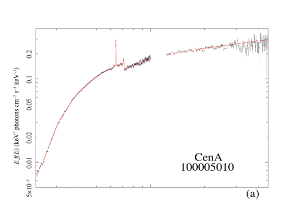
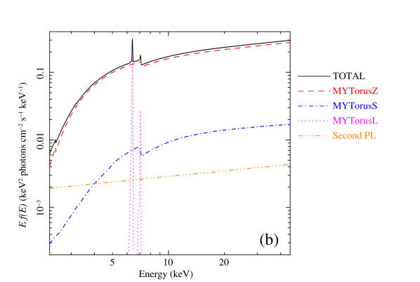
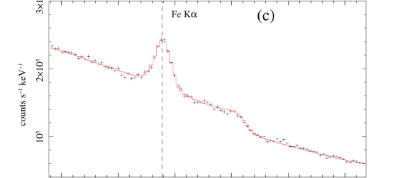
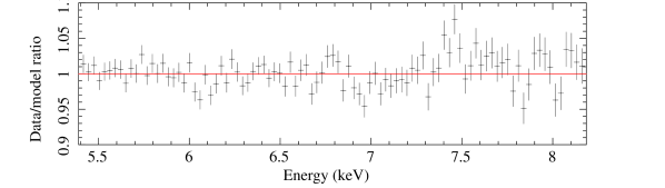
Figure B.1: CenA 100005010

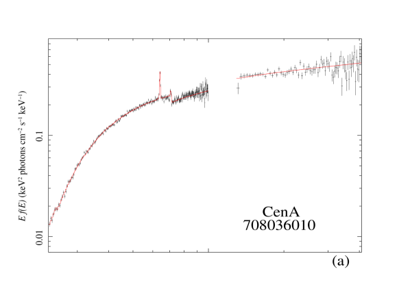
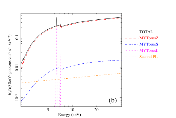
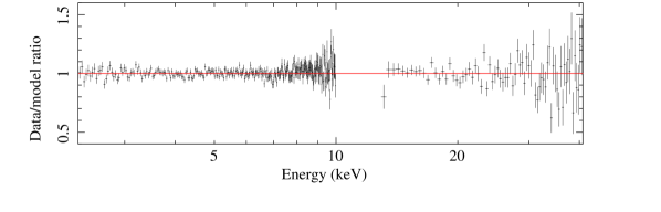
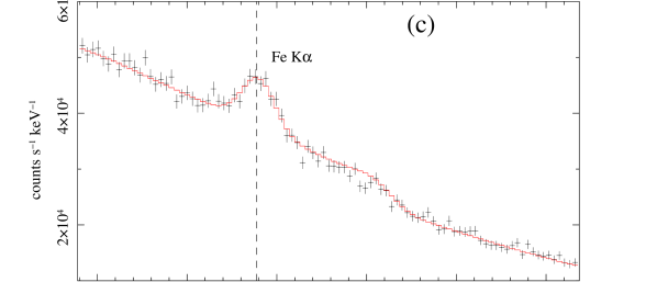
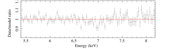
Figure B.2: CenA 708036010

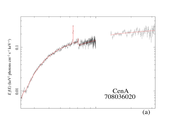
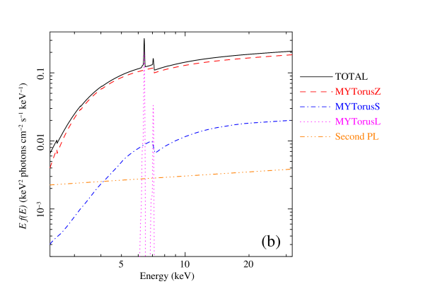
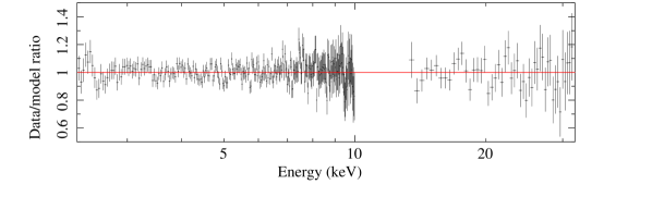
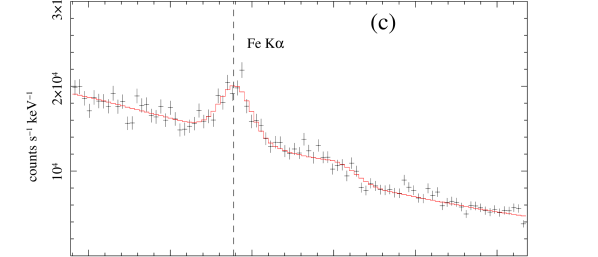
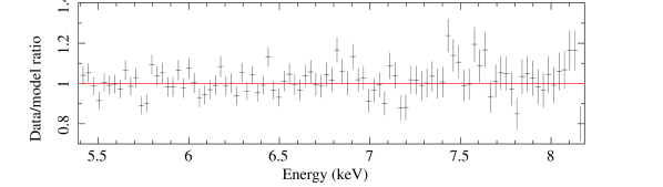
Figure B.3: CenA 708036020

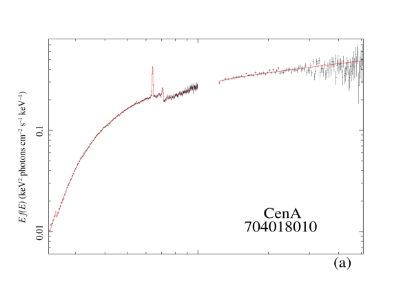
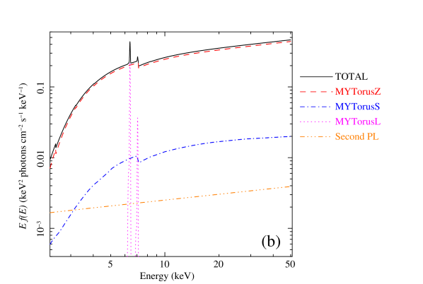
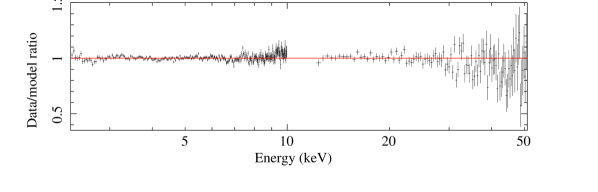
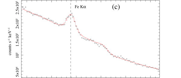
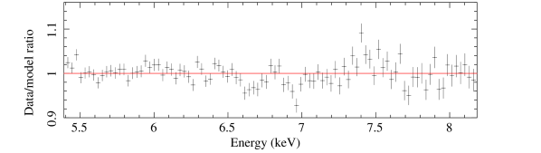
Figure B.4: CenA 704018010

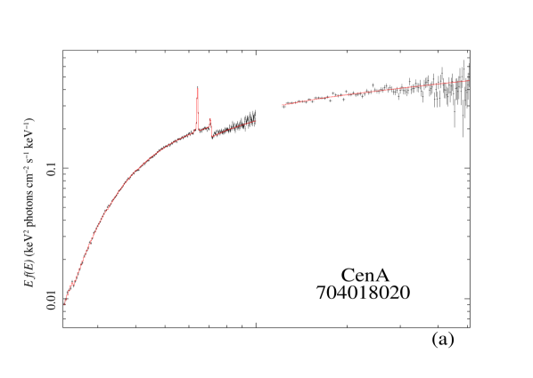
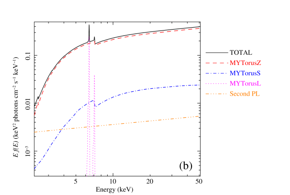
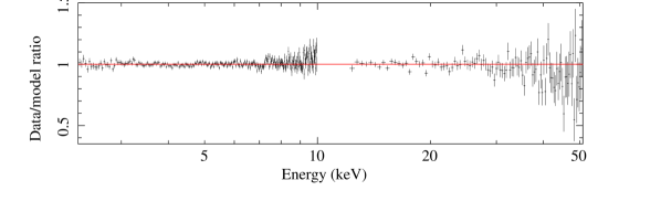
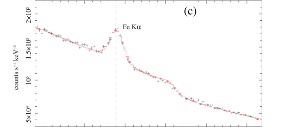
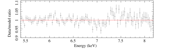
Figure B.5: CenA 704018020

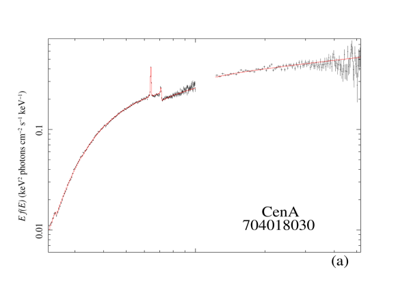
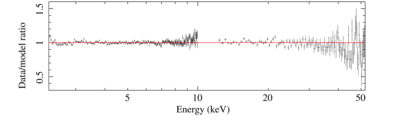
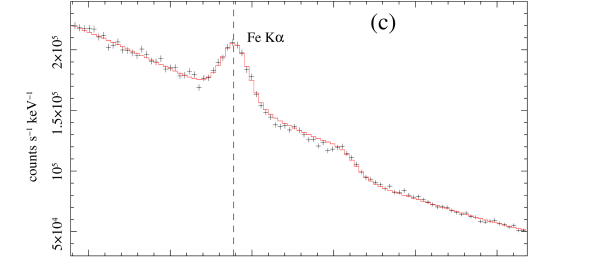
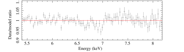
Figure B.6: CenA 704018030

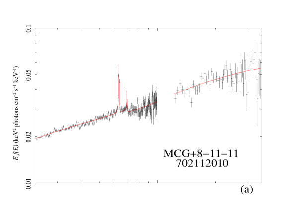
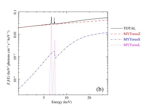
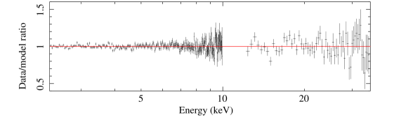
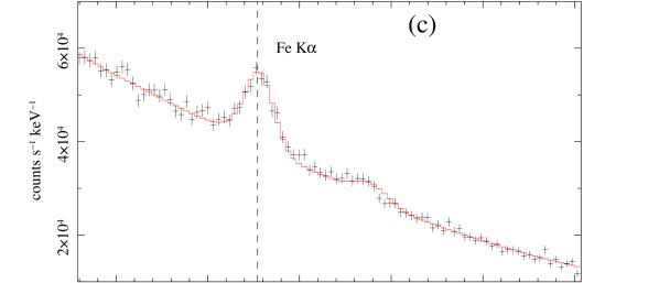
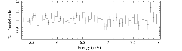
Figure B.7: MCG+8-11-11 702112010

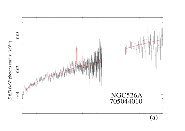
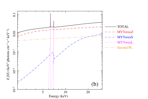
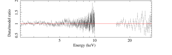
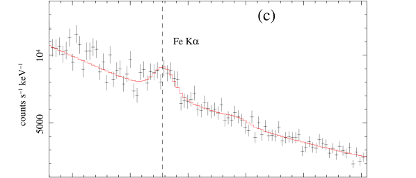
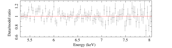
Figure B.8: NGC526A 705044010

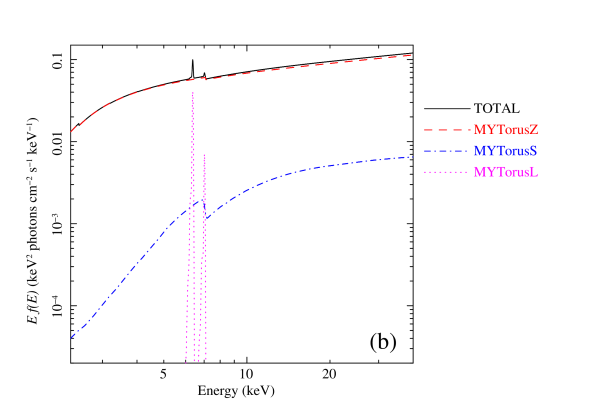
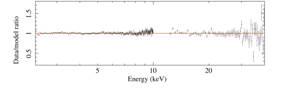
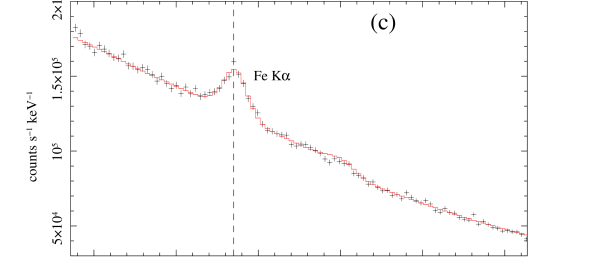
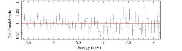
Figure B.9: NGC2110 100024010

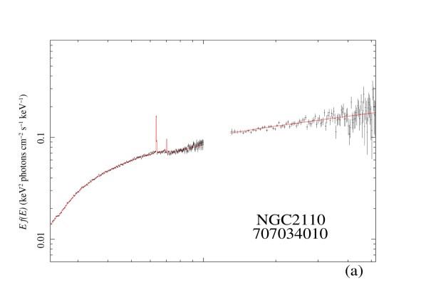
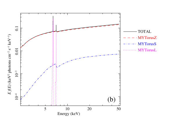
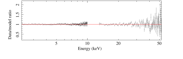
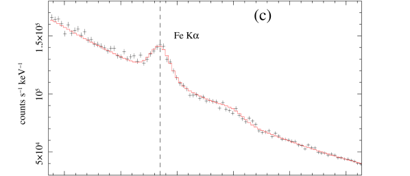
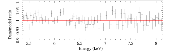
Figure B.10: NGC2110 707034010

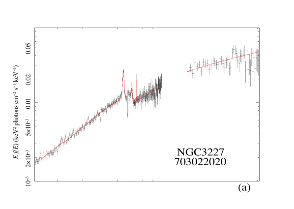
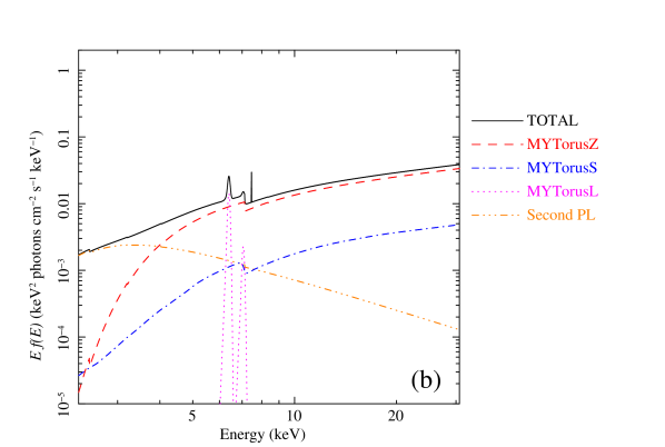
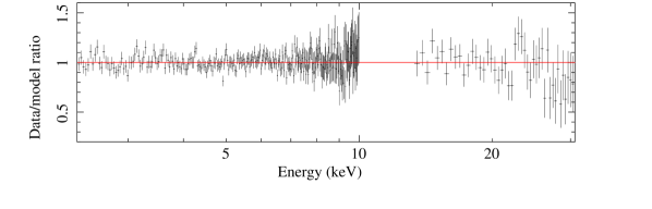
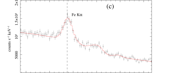
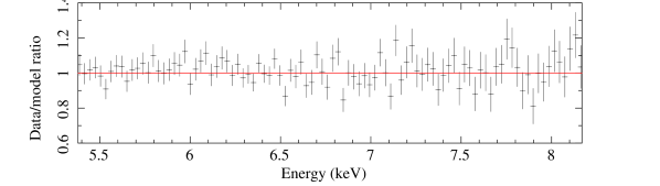
Figure B.11: NGC3227 703022020

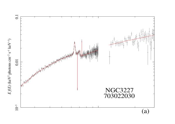
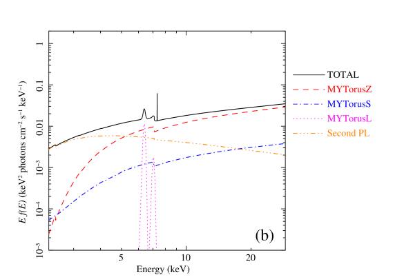
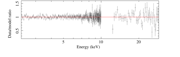
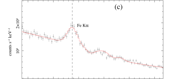
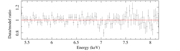
Figure B.12: NGC3227 703022030

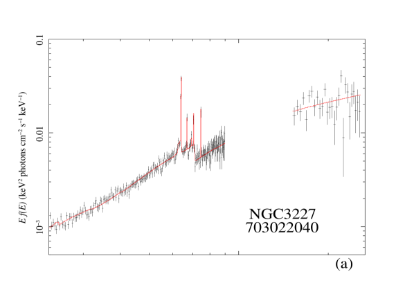
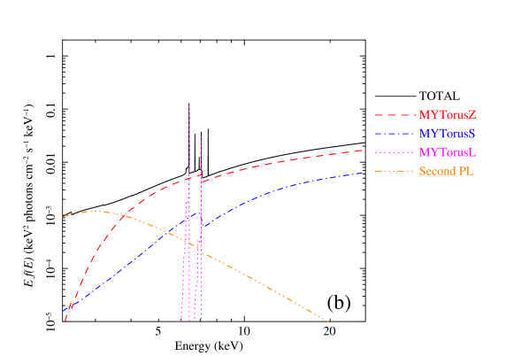
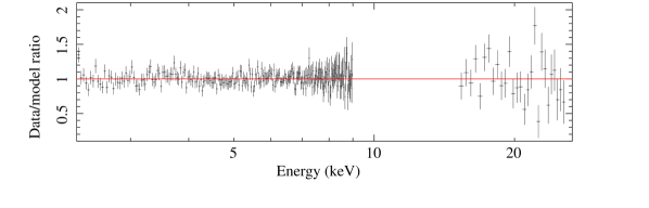
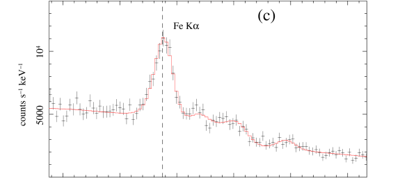
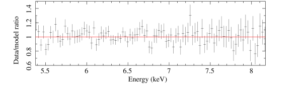
Figure B.13: NGC3227 703022040

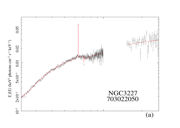
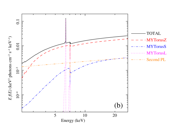
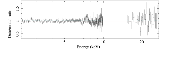
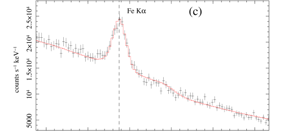
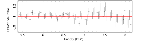
Figure B.14: NGC3227 703022050

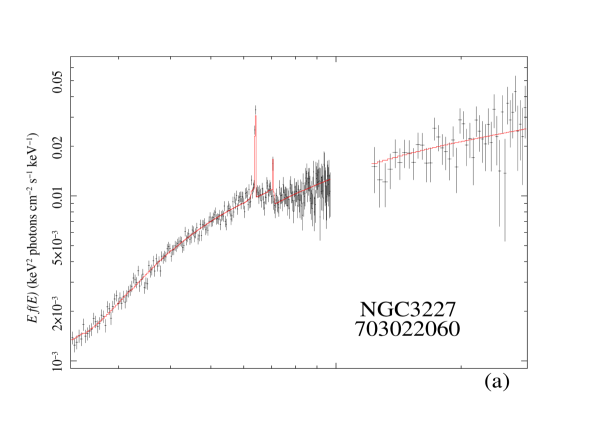
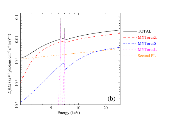
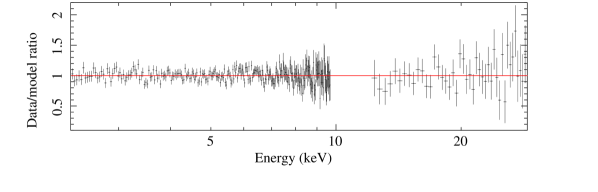
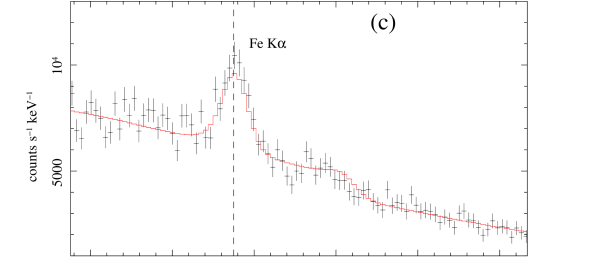
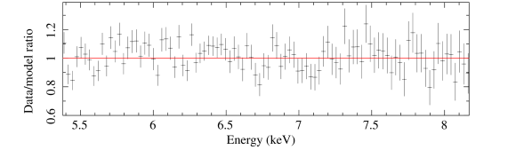
Figure B.15: NGC3227 703022060

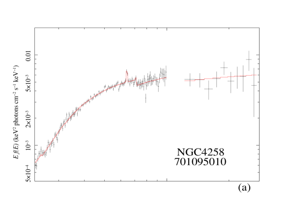
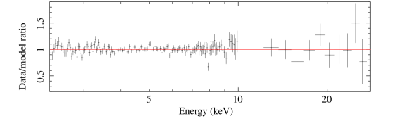
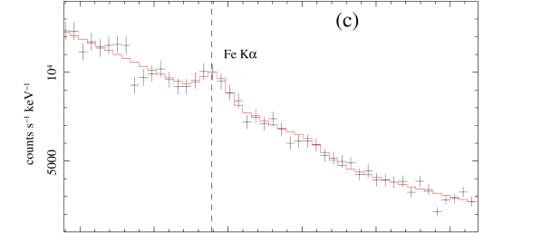
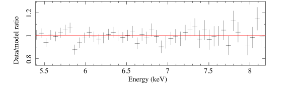
Figure B.16: NGC4258 701095010

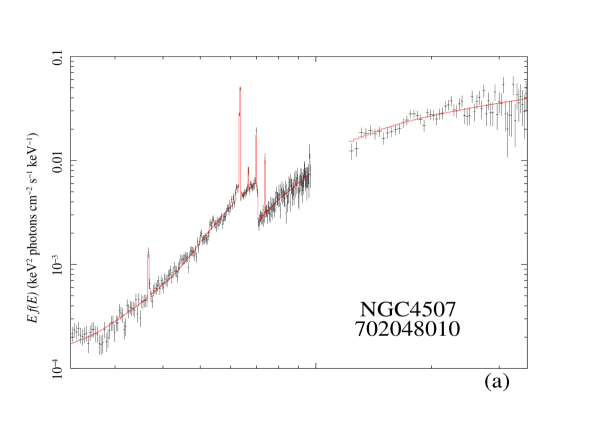
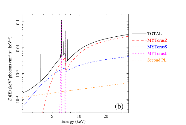
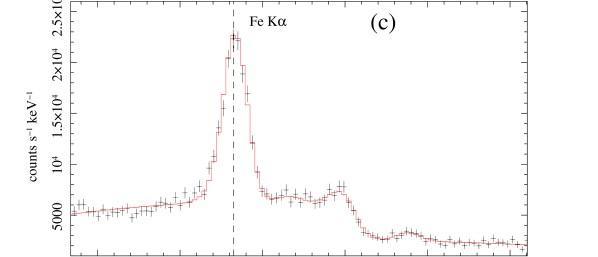
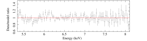
Figure B.17: NGC4507 702048010

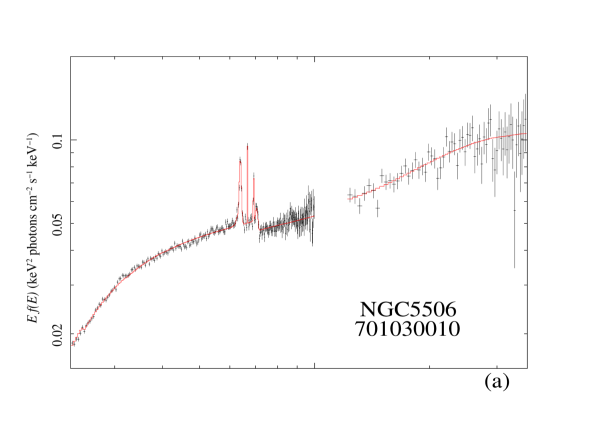
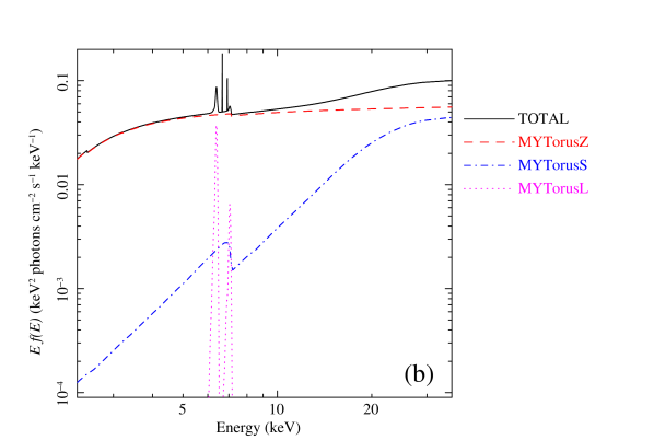
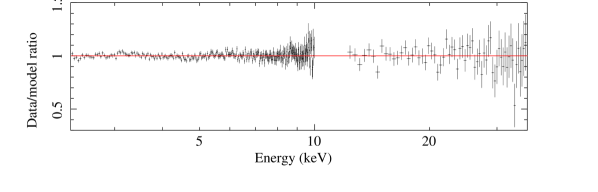
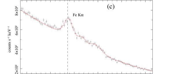
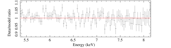
Figure B.18: NGC5506 701030010

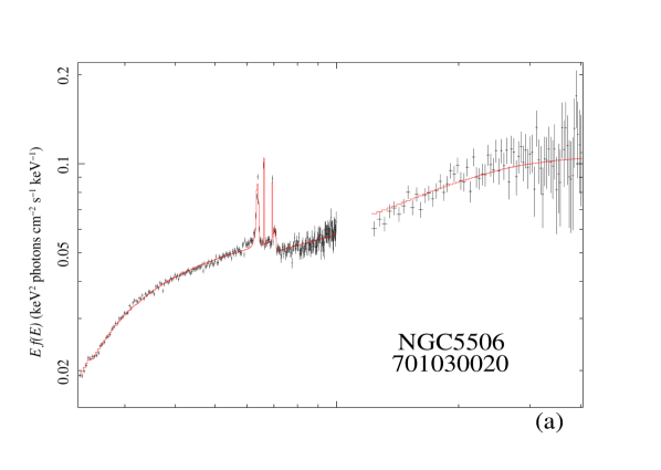
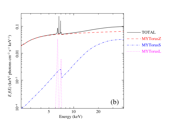
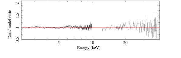
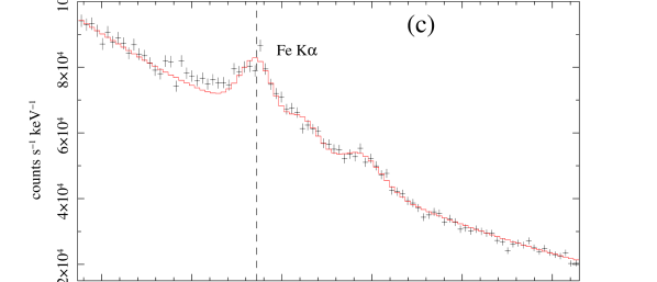
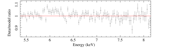
Figure B.19: NGC5506 701030020

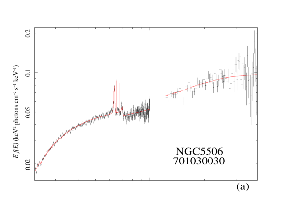
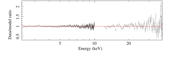
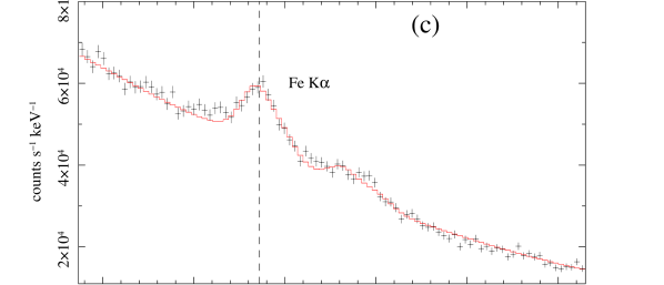
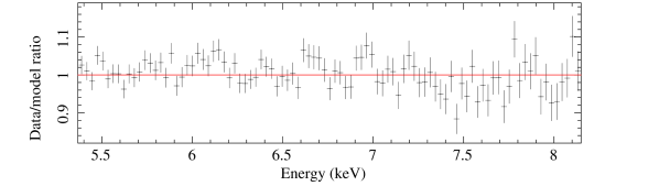
Figure B.20: NGC5506 701030030

References

- Alonso-Herrero et al. (2019) Alonso-Herrero, A., García-Burillo, S., Pereira-Santaella, M., et al. 2019, A&A, 628, A65
- Anders & Grevesse (1989) Anders, E., & Grevesse, N. 1989, Geochim. Cosmochim. Acta, 53, 197
- Arnaud (1996) Arnaud, K. A. 1996, in Astronomical Society of the Pacific Conference Series, Vol. 101, Astronomical Data Analysis Software and Systems V, ed. G. H. Jacoby & J. Barnes, 17
- Baronchelli et al. (2018) Baronchelli, L., Nandra, K., & Buchner, J. 2018, MNRAS, 480, 2377
- Beuchert et al. (2015) Beuchert, T., Markowitz, A. G., Krauß, F., et al. 2015, A&A, 584, A82
- Bianchi et al. (2003) Bianchi, S., Balestra, I., Matt, G., Guainazzi, M., & Perola, G. C. 2003, A&A, 402, 141
- Bianchi et al. (2010) Bianchi, S., de Angelis, I., Matt, G., et al. 2010, A&A, 522, A64
- Blandford & Znajek (1977) Blandford, R. D., & Znajek, R. L. 1977, MNRAS, 179, 433
- Braito et al. (2013) Braito, V., Ballo, L., Reeves, J. N., et al. 2013, MNRAS, 428, 2516
- Brenneman (2013) Brenneman, L. 2013, Springer Briefs in Astronomy. ISBN 978-1-4614-7770-9, doi:10.1007/978-1-4614-7771-6
- Brenneman & Reynolds (2009) Brenneman, L. W., & Reynolds, C. S. 2009, ApJ, 702, 1367
- Crook et al. (2007) Crook, A. C., Huchra, J. P., Martimbeau, N., et al. 2007, ApJ, 655, 790
- Davies et al. (2014) Davies, R. I., Maciejewski, W., Hicks, E. K. S., et al. 2014, ApJ, 792, 101
- de la Calle Pérez et al. (2010) de la Calle Pérez, I., Longinotti, A. L., Guainazzi, M., et al. 2010, A&A, 524, A50
- Elitzur & Shlosman (2006) Elitzur, M., & Shlosman, I. 2006, ApJ, 648, L101
- Esin et al. (1997) Esin, A. A., McClintock, J. E., & Narayan, R. 1997, ApJ, 489, 865
- Evans et al. (2004) Evans, D. A., Kraft, R. P., Worrall, D. M., et al. 2004, ApJ, 612, 786
- Evans et al. (2007) Evans, D. A., Lee, J. C., Turner, T. J., Weaver, K. A., & Marshall, H. L. 2007, ApJ, 671, 1345
- Fukazawa et al. (2011a) Fukazawa, Y., Hiragi, K., Mizuno, M., et al. 2011a, ApJ, 727, 19
- Fukazawa et al. (2011b) Fukazawa, Y., Hiragi, K., Yamazaki, S., et al. 2011b, ApJ, 743, 124
- Garcia (1993) Garcia, A. M. 1993, A&AS, 100, 47
- García et al. (2016) García, J. A., Fabian, A. C., Kallman, T. R., et al. 2016, MNRAS, 462, 751
- George & Fabian (1991) George, I. M., & Fabian, A. C. 1991, MNRAS, 249, 352
- Giacconi et al. (1962) Giacconi, R., Gursky, H., Paolini, F. R., & Rossi, B. B. 1962, Phys. Rev. Lett., 9, 439
- Gilli et al. (2007) Gilli, R., Comastri, A., & Hasinger, G. 2007, A&A, 463, 79
- Graham (2016) Graham, A. W. 2016, in Astrophysics and Space Science Library, Vol. 418, Galactic Bulges, ed. E. Laurikainen, R. Peletier, & D. Gadotti, 263
- Guainazzi et al. (2006) Guainazzi, M., Bianchi, S., & Dovčiak, M. 2006, \anach, 327, 1032
- Guainazzi et al. (2010) Guainazzi, M., Bianchi, S., Matt, G., et al. 2010, MNRAS, 406, 2013
- HI4PI Collaboration et al. (2016) HI4PI Collaboration, Ben Bekhti, N., Flöer, L., et al. 2016, A&A, 594, A116
- Hönig et al. (2013) Hönig, S. F., Kishimoto, M., Tristram, K. R. W., et al. 2013, ApJ, 771, 87
- Jiménez-Bailón et al. (2005) Jiménez-Bailón, E., Piconcelli, E., Guainazzi, M., et al. 2005, A&A, 435, 449
- Koyama et al. (2007) Koyama, K., Tsunemi, H., Dotani, T., et al. 2007, PASJ, 59, 23
- Laha et al. (2020) Laha, S., Markowitz, A. G., Krumpe, M., et al. 2020, ApJ, 897, 66
- LaMassa et al. (2014) LaMassa, S. M., Yaqoob, T., Ptak, A. F., et al. 2014, ApJ, 787, 61
- Lamer et al. (2003) Lamer, G., Uttley, P., & McHardy, I. M. 2003, MNRAS, 342, L41
- Landi et al. (2001) Landi, R., Bassani, L., Malaguti, G., et al. 2001, A&A, 379, 46
- Liu & Li (2015) Liu, Y., & Li, X. 2015, MNRAS, 448, L53
- Lobban et al. (2020) Lobban, A. P., Turner, T. J., Reeves, J. N., Braito, V., & Miller, L. 2020, MNRAS, 494, 5056
- Lohfink et al. (2012) Lohfink, A. M., Reynolds, C. S., Miller, J. M., et al. 2012, ApJ, 758, 67
- Madsen et al. (2017) Madsen, K. K., Beardmore, A. P., Forster, K., et al. 2017, AJ, 153, 2
- Mantovani et al. (2016) Mantovani, G., Nandra, K., & Ponti, G. 2016, MNRAS, 458, 4198
- Markowitz et al. (2009) Markowitz, A., Reeves, J. N., George, I. M., et al. 2009, ApJ, 691, 922
- Markowitz et al. (2007) Markowitz, A., Takahashi, T., Watanabe, S., et al. 2007, ApJ, 665, 209
- Markowitz et al. (2014) Markowitz, A. G., Krumpe, M., & Nikutta, R. 2014, MNRAS, 439, 1403
- Matt et al. (2006) Matt, G., Bianchi, S., de Rosa, A., Grandi, P., & Perola, G. C. 2006, A&A, 445, 451
- Mitsuda et al. (2007) Mitsuda, K., Bautz, M., Inoue, H., et al. 2007, PASJ, 59, S1
- Mulchaey et al. (1997) Mulchaey, J. S., Regan, M. W., & Kundu, A. 1997, ApJS, 110, 299
- Mundell et al. (2004) Mundell, C. G., James, P. A., Loiseau, N., Schinnerer, E., & Forbes, D. A. 2004, ApJ, 614, 648
- Mundell et al. (1995) Mundell, C. G., Pedlar, A., Axon, D. J., Meaburn, J., & Unger, S. W. 1995, MNRAS, 277, 641
- Murphy & Nowak (2014) Murphy, K. D., & Nowak, M. A. 2014, ApJ, 797, 12
- Murphy & Yaqoob (2009) Murphy, K. D., & Yaqoob, T. 2009, MNRAS, 397, 1549
- Nandra (2006) Nandra, K. 2006, MNRAS, 368, L62
- Nandra et al. (2007) Nandra, K., O’Neill, P. M., George, I. M., & Reeves, J. N. 2007, MNRAS, 382, 194
- Narayan & Yi (1994) Narayan, R., & Yi, I. 1994, ApJ, 428, L13
- Nenkova et al. (2008) Nenkova, M., Sirocky, M. M., Nikutta, R., Ivezić, Ž., & Elitzur, M. 2008, ApJ, 685, 160
- Netzer et al. (1990) Netzer, H., Maoz, D., Laor, A., et al. 1990, ApJ, 353, 108
- Noda et al. (2014) Noda, H., Makishima, K., Yamada, S., et al. 2014, ApJ, 794, 2
- Patrick et al. (2012) Patrick, A. R., Reeves, J. N., Porquet, D., et al. 2012, MNRAS, 426, 2522
- Porquet et al. (2004) Porquet, D., Reeves, J. N., O’Brien, P., & Brinkmann, W. 2004, A&A, 422, 85
- Ricci et al. (2015) Ricci, C., Ueda, Y., Koss, M. J., et al. 2015, ApJ, 815, L13
- Ricci et al. (2014) Ricci, C., Ueda, Y., Paltani, S., et al. 2014, MNRAS, 441, 3622
- Risaliti et al. (2007) Risaliti, G., Elvis, M., Fabbiano, G., et al. 2007, ApJ, 659, L111
- Risaliti et al. (2002) Risaliti, G., Elvis, M., & Nicastro, F. 2002, ApJ, 571, 234
- Shu et al. (2010) Shu, X. W., Yaqoob, T., & Wang, J. X. 2010, ApJS, 187, 581
- Shu et al. (2011) Shu, X. W., Yaqoob, T., & Wang, J. X. 2011, ApJ, 738, 147
- Sun et al. (2018) Sun, S., Guainazzi, M., Ni, Q., et al. 2018, MNRAS, 478, 1900
- Takahashi et al. (2007) Takahashi, T., Abe, K., Endo, M., et al. 2007, PASJ, 59, 35
- Tortosa et al. (2018) Tortosa, A., Bianchi, S., Marinucci, A., et al. 2018, MNRAS, 473, 3104
- Tsujimoto et al. (2011) Tsujimoto, M., Guainazzi, M., Plucinsky, P. P., et al. 2011, A&A, 525, A25
- Turner et al. (2018) Turner, T. J., Reeves, J. N., Braito, V., et al. 2018, MNRAS, 481, 2470
- Turner et al. (2020) Turner, T. J., Reeves, J. N., Braito, V., et al. 2020, MNRAS, 498, 1983
- Tzanavaris et al. (2019) Tzanavaris, P., Yaqoob, T., LaMassa, S., Yukita, M., & Ptak, A. 2019, ApJ, 885, 62
- Ueda et al. (2014) Ueda, Y., Akiyama, M., Hasinger, G., Miyaji, T., & Watson, M. G. 2014, ApJ, 786, 104
- Verner et al. (1996) Verner, D. A., Ferland, G. J., Korista, K. T., & Yakovlev, D. G. 1996, ApJ, 465, 487
- Yaqoob (2012) Yaqoob, T. 2012, MNRAS, 423, 3360
- Yaqoob & Murphy (2011) Yaqoob, T., & Murphy, K. D. 2011, MNRAS, 412, 277
- Yaqoob & Padmanabhan (2004) Yaqoob, T., & Padmanabhan, U. 2004, ApJ, 604, 63
- Yaqoob et al. (2015) Yaqoob, T., Tatum, M. M., Scholtes, A., Gottlieb, A., & Turner, T. J. 2015, MNRAS, 454, 973
- Yaqoob et al. (2016) Yaqoob, T., Turner, T. J., Tatum, M. M., Trevor, M., & Scholtes, A. 2016, MNRAS, 462, 4038
- Zoghbi et al. (2020) Zoghbi, A., Kalli, S., Miller, J. M., & Mizumoto, M. 2020, ApJ, 893, 97
- Zoghbi et al. (2019) Zoghbi, A., Miller, J. M., & Cackett, E. 2019, ApJ, 884, 26