Weisfeiler-Leman in the Bamboo: Novel AMR Graph Metrics
and a Benchmark for AMR Graph Similarity

Abstract

Several metrics have been proposed for assessing the similarity of (abstract) meaning representations (AMRs), but little is known about how they relate to human similarity ratings. Moreover, the current metrics have complementary strengths and weaknesses: some emphasize speed, while others make the alignment of graph structures explicit, at the price of a costly alignment step.

In this work we propose new Weisfeiler-Leman AMR similarity metrics that unify the strengths of previous metrics, while mitigating their weaknesses. Specifically, our new metrics are able to match contextualized substructures and induce n:m alignments between their nodes. Furthermore, we introduce a Benchmark for AMR Metrics based on Overt Objectives (Bamboo), the first benchmark to support empirical assessment of graph-based MR similarity metrics. Bamboo maximizes the interpretability of results by defining multiple overt objectives that range from sentence similarity objectives to stress tests that probe a metric’s robustness against meaning-altering and meaning-preserving graph transformations. We show the benefits of Bamboo by profiling previous metrics and our own metrics. Results indicate that our novel metrics may serve as a strong baseline for future work.

1 Introduction

Meaning representations aim at capturing the meaning of text in an explicit graph format. A prominent framework is abstract meaning representation (AMR), proposed by Banarescu et al. (2013). AMR views sentences as rooted, directed, acyclic, labeled graphs. Their nodes are variables, attributes or (open-class) concepts and are connected with edges that express semantic relations.

There are many use cases in which we need to compare or relate two AMR graphs. A common situation is found in parser evaluation, where AMR metrics are widely applied May (2016); May and Priyadarshi (2017). Yet, there are more situations where we need to measure similarity of meaning as expressed in AMR graphs. E.g., Bonial et al. (2020) leverage AMR metrics in a semantic search engine for COVID-19 queries, Naseem et al. (2019) use metric feedback to reinforce AMR parsers, Opitz (2020) emulates metrics for referenceless AMR ranking and rating, and Opitz and Frank (2021) employ AMR metrics for NLG evaluation.

So far, multiple AMR metrics Cai and Knight (2013); Cai and Lam (2019); Song and Gildea (2019); Anchiêta et al. (2019); Opitz et al. (2020) have been proposed to assess AMR similarity. However, due to a lack of an appropriate evaluation benchmark, we have no empirical evidence that could tell us more about their strengths and weaknesses or offer insight about which metrics may be preferable over others in specific use cases.

Additionally, we would like to move beyond the aforementioned metrics and develop new metrics that account for graded similarity of graph substructures, which is

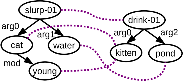
Figure 1: Similar AMRs, with sketched alignments.

not an easy task. However, it is crucial when we need to compare AMR graphs in a deeper way. Consider Fig. 1, which shows two AMRs that convey very similar meanings. All aforementioned metrics assign this pair a low similarity score, and – if alignment-based, as is Smatch Cai and Knight (2013) – find only subpar alignments. In this case, we want a metric that provides us with a high similarity score and, ideally, an explanatory alignment.

The structure of this paper is as follows. In §2 we discuss related work. In §3 we describe our first contribution: new AMR metrics that aim at unifying the strengths of previous metrics while mitigating their weaknesses. Specifically, our new metrics are capable of matching larger substructures and provide valuable n-m alignments in polynomial time. In §4 we introduce Bamboo, our second contribution: it is the first benchmark data set for AMR metrics and includes novel robustness objectives that probe the behavior of AMR metrics under meaning-preserving and meaning-altering transformations of the inputs (§5). In §6 we use Bamboo for a detailed, multi-faceted empirical study of previous and our proposed AMR metrics.

We release Bamboo and our new metrics.

2 Related work

The classical AMR metric and its adaptions.

The ‘canonical’ and widely applied AMR metric is Smatch (Semantic match) (Cai and Knight, 2013). It solves an NP-hard graph alignment problem approximately with a hill-climber and scores matching triples. Smatch has been adapted to S²match (Soft Semantic match), by Opitz et al. (2020) to account for graded similarity of concept nodes (e.g., cat – kitten), using word embeddings. Smatch has also been adapted by Cai and Lam (2019) in W(eighted)Smatch (WSmatch), which penalizes errors relative to their distance to the root. This is motivated by the hypothesis that “core semantics” tend to be located near a graph’s root.

BFS-based and alignment-free AMR metrics

Recently, two new AMR metrics have been proposed: Sema by Anchiêta et al. (2019) and SemBleu by Song and Gildea (2019). Common to both is a mechanism that traverses the graph. Both start from the root, and collect structures with a breadth-first traversal (BFS). Also, both ablate the variable alignment of (W)S⁽²⁾match and only consider their attached concepts, which increases computation speed. Apart from this, the metrics differ significantly: SemBleu extracts bags of k-hop paths (k$\leq$3) from the AMR graphs and thereupon calculates BLEU Papineni et al. (2002). Sema, on the other hand, is somewhat simpler and provides us with an F1 score that it achieves by comparing extracted triples.

From measuring structure overlap to measuring meaning similarity

Most AMR metrics have been designed for semantic parser evaluation, and therefore determine a score for structure overlap. While this is legitimate, with extended use cases for AMR metrics arising, there is increased awareness that structural matching of labeled nodes and edges of an AMR graph is not sufficient for assessing the meaning similarity expressed by two AMRs Kapanipathi et al. (2021). This insufficiency has also been observed in cross-lingual AMR parsing evaluation Blloshmi et al. (2020); Sheth et al. (2021); Uhrig et al. (2021), but is most prominent when attempting to compare the meaning of AMRs that represent different sentences Opitz et al. (2020); Opitz and Frank (2021). This work argues that in cases like Fig. 1, the available metrics do not sufficiently reflect the similarity of the two AMRs and their underlying sentences.

How do humans rate similarity of sentence meaning?

STS Baudiš et al. (2016a, b); Cer et al. (2017) and SICK Marelli et al. (2014) elicited human ratings of sentence similarity on a Likert scale. While STS annotates semantic similarity, SICK annotates semantic relatedness. These two aspects are highly related, but not the exact same Budanitsky and Hirst (2006); Kolb (2009). Only the highest scores on the Likert scales of SICK and STS can be seen as reflecting the equivalence of meaning of two sentences. Other data sets contain binary annotations of paraphrases Dolan and Brockett (2005), that cover a wide spectrum of semantic phenomena.

Benchmarking Metrics

Metric benchmarking is an active topic in NLP research and led to the emergence of metric benchmarks in various areas, most prominently, MT and NLG Gardent et al. (2017); Zhu et al. (2018); Ma et al. (2019). These benchmarks are useful since they help to assess and select metrics and encourage their further development Gehrmann et al. (2021). However, there is currently no established benchmark that defines a ground truth of graded semantic similarity between pairs of AMRs, and how to measure it in terms of their structural representations. Also, we do not have an established ground truth to assess what alternative AMR metrics such as (W|S²)match or SemBleu really measure, and how their scores correlate with human judgments of the semantic similarity of sentences represented by AMRs.

3 Grounding novel AMR metrics in Weisfleiler-Leman graph kernel

Previous AMR metrics have complementary strengths and weaknesses. Therefore, we aim to propose new AMR metrics that are able to mitigate these weaknesses, while unifying their strengths, aiming at the best of all worlds. We want:

1. an interpretable alignment (Smatch);
   

2. a fast metric (Sema, SemBleu);
   

3. matching larger substructures (SemBleu)
   

4. and assessment of graded similarity of AMR subgraphs (extending S²match).

This section proposes to make use of the Weisfeiler-Leman graph kernel (WLK) Weisfeiler and Leman (1968); Shervashidze et al. (2011) to assess AMR similarity. The idea is that WLK provides us with SemBleu-like matches of larger sub-structures, while bypassing potential biases induced by the BFS-traversal Opitz et al. (2020). We then describe the Wasserstein Weisfeiler Leman kernel (WWLK) Togninalli et al. (2019) that is similar to WLK but provides i) an alignment of atomic and non-atomic substructures (going beyond Smatch) and ii) a graded match of substructures (going beyond S²match). Finally, we further adapt WWLK to WWLK_Θ, a variant that we tailor to learn semantic edge parameters, to better assess AMR graphs.

3.1 Basic Weisfeiler-Leman Kernel (WLK)

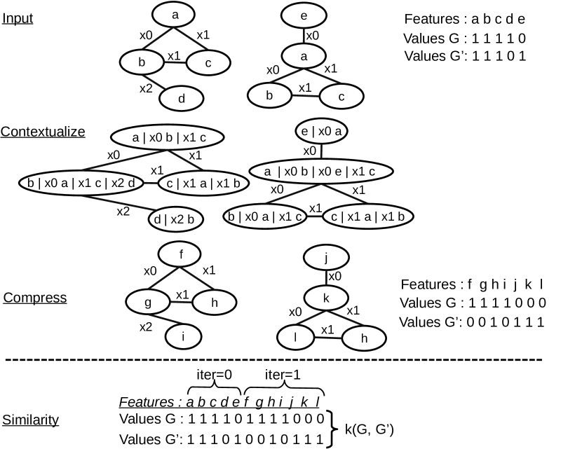
Figure 2: WLK example based on one iteration.

The Weisfeiler-Leman kernel (WLK) method Shervashidze et al. (2011) derives sub-graph features from two input graphs. WLK has shown its power in many tasks, ranging from protein classification to movie recommendation Togninalli et al. (2019); Yanardag and Vishwanathan (2015). However, so far, it has not been applied to (A)MR graphs. In the following, we will describe the WLK method.

Generally, a kernel can be viewed as a similarity measurement between two objects Hofmann et al. (2008), in our case, two AMR graphs $\mathcal{G},\mathcal{G}^{\prime}$. It is stated as $\mathbf{k}(\mathcal{G},\mathcal{G}^{\prime})=\langle\Phi(\mathcal{G}),\Phi(\mathcal{G}^{\prime})\rangle$ where $\langle\cdot,\cdot\rangle:\mathbb{R}^{d}\times\mathbb{R}^{d}\rightarrow\mathbb{R}_{+}$ is an inner product and $\Phi$ maps an input to a feature vector that is built incrementally over $K$ iterations. For our AMR graphs, one such iteration $k$ works as follows: a) every node receives the labels of its neighbors and the labels of the edges connecting it to their neighbors, and stores them in a list (cf. Contextualize in Fig. 2). b) The lists are alphabetically sorted and the string elements of the lists are concatenated to form new aggregate labels (cf. Compress in Fig. 2). c) Two count vectors $x_{\mathcal{G}}^{k}$ and $x_{\mathcal{G}^{\prime}}^{k}$ are created where each dimension corresponds to a node label that is found in any of the two graphs and contains its count (cf. Features in Fig. 2). Since every iteration yields two vectors (one for each input), we can concatenate the vectors over iterations and calculate the kernel (cf. Similarity in Fig. 2):

$$\mathbf{k}(\cdot,\cdot) =\langle\Phi_{WL}(\mathcal{G}),\Phi_{WL}(\mathcal{G}^{\prime})\rangle$$ (1)

$$=\langle concat(x_{\mathcal{G}}^{0},...,x_{\mathcal{G}}^{K}),concat(x_{\mathcal{G}^{\prime}}^{0},...,x_{\mathcal{G^{\prime}}}^{K}\rangle$$

Specifically, we use the cosine similarity kernel and two iterations ($K$=2), which implies that every node receives information from its neighbors and their immediate neighbors. For simplicity we will first treat edges as undirected, but later will experiment with various directionality parameterizations.

3.2 Wasserstein Weisfeiler-Leman (WWLK)

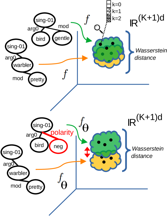
Figure 3: Wasserstein WLK example w/o learned edge parameters (top, §3.2) and w/ learnt edge parameters (bottom, §3.3), which allow us to adjust the embedded graphs such that they better take the (impact of) AMR edges into account. Red: the distance increases because of a negation contrast between the two AMRs that otherwise convey similar meaning.

S²match differs from all other AMR metrics in that it accepts close concept synonyms for alignment (up to a similarity threshold). But it comes with a restriction and a downside: i) it cannot assess graded similarity of (non-atomic) AMR subgraphs, which is crucial for assessing partial meaning agreement between AMRs (as illustrated in Fig. 1), and ii) the alignment is costly to compute.

We hence propose to adopt a variant of WLK: the Wasserstein-Weisfeiler Leman kernel (WWLK) Togninalli et al. (2019) for the following two reasons: i) WWLK can assess non-atomic subgraphs on a finer level, and ii) it provides graph alignments that are faster to compute than any of the existing Smatch metrics: (W)S⁽²⁾match.

WWLK works in two steps: 1. given its initial node embeddings, we use WL to project the graph into a latent space, in which the final node embeddings describe varying degrees of contextualization. 2. given a pair of such (WL) embedded graphs, a transportation plan is found that describes the minimum cost of transforming one graph into the other. In the top graph of Fig. 3, $f$ indicates the first step, while Wasserstein distance indicates the second. Now, we describe the steps in closer detail.

Step 1: WL graph projection into latent space

Let $v=1...n$ be the nodes of AMR $\mathcal{G}$. This graph is projected onto a matrix $\mathbb{R}^{n}\times\mathbb{R}^{(K+1)d}$ with

$$f(\mathcal{G}) =hStack(X_{\mathcal{G}}^{0},...,X_{\mathcal{G}}^{K}),\text{where}$$ (2)

$$X_{\mathcal{G}}^{k} =[x^{k}(1),...,x^{k}(n)]^{T}\in\mathbb{R}^{n}\times\mathbb{R}^{d}.$$ (3)

$hstack$ concatenates matrices s.t. $(\big{[}\begin{smallmatrix}a&b\\ c&d\end{smallmatrix}\big{]},\big{[}\begin{smallmatrix}x&y\\ w&z\end{smallmatrix}\big{]})\rightarrow\big{[}\begin{smallmatrix}a&b&x&y\\ c&d&w&z\end{smallmatrix}\big{]}$. This means that, in the output space, every node is associated with a vector that is itself a concatenation of $K+1$ vectors with $d$ dimensions each, where $k$ indicates the degree of contextualization ( in Fig. 3). The embedding $x(v)^{k}\in\mathbb{R}^{d}$ for a node $v$ in a certain iteration $k$ is computed as follows:

$$x(v)^{k+1}=\frac{1}{2}\bigg{(}x(v)^{k}+\frac{1}{d(v)}\sum_{u\in\mathcal{N}_{v}}w(u,v)\cdot x(u)^{k}\bigg{)}.$$ (4)

$d(v)$ is the degree of a node, $\mathcal{N}$ returns the neighbors for a node, $w(u,v)$ can assign a weight to a node pair. The initial node embeddings, i.e., $x(\cdot)^{0}$, can be set up by looking up the node labels in a set of pre-trained word embeddings, or using random initialization. To distinguish between the discrete edge labels, we sample random weights.

Step 2: Computing the Wasserstein distance between two WL-embedded graphs

The Wasserstein distance describes the minimum amount of work that is necessary to transform the (contextualized) nodes of one graph into the (contextualized) nodes of the other. It is computed based on pairwise euclidean distances from $f(\mathcal{G})$ with $n$ nodes, and $f(\mathcal{G}^{\prime})$ with $m$ nodes:

$$distance=\sum_{i=1}^{n}\sum_{j=1}^{m}\mathbf{T}_{i,j}D_{i,j}$$ (5)

Here, the ‘cost matrix’ $D\in\mathbb{R}^{n\times m}$ contains the euclidean distances between the $n$ WL-embedded nodes from $\mathcal{G}$ and $m$ WL-embedded nodes from $\mathcal{G^{\prime}}$. I.e., $D_{i,j}=||f(\mathcal{G})_{i}-f(\mathcal{G}^{\prime})_{j}||_{2}$. The flow matrix $\mathbf{T}$ describes a transportation plan between the two graphs, i.e, $\mathbf{T}_{i,j}\geq 0$ states how much of node $i$ from $\mathcal{G}$ flows to node $j$ from $\mathcal{G}^{\prime}$, the corresponding ‘local work’ can be stated as $flow(i,j)\cdot cost(i,j):=\mathbf{T}_{i,j}\cdot D_{i,j}$. To find the best $\mathbf{T}$, i.e., the transportation plan that minimizes the cumulative work needed (Eq. 5), we solve a constraint linear problem:

$$\min \sum_{i=1}^{n}\sum_{j=1}^{m}\mathbf{T}_{i,j}D_{i,j}$$ (6)

$$s.t.:~{}~{} \mathbf{T}_{i,j}\geq 0,1\leq i\leq n,1\leq j\leq m$$ (7)

$$\sum_{j=1}^{m}{\mathbf{T}_{i,j}}=\frac{1}{m},1\leq i\leq n$$ (8)

$$\sum_{i=1}^{n}{\mathbf{T}_{i,j}}=\frac{1}{n},1\leq j\leq m$$ (9)

Note that i) the transportation plan $\mathbf{T}$ describes an n:m alignment between the nodes of the two graphs, and that ii) solving Eq. 6 has polynomial time complexity, while the (W)S⁽²⁾match problem is NP-complete.

3.3 From WWLK to WWLK_θ with zero^th-order optimization

Motivation: AMR edge labels have meaning

The WL-embedding mechanism of WWLK (Eq. 4) associates a weight $w(u,v)\in\mathbb{R}$ with each edge. For unlabeled graphs, $w(u,v)$ is simply set to one. To distinguish between the discrete AMR edge labels, in WWLK we have used random weights. However, AMR edge labels encode complex relations between nodes, and simply choosing random weights may not be enough. In fact, we hypothesize that different edge labels may impact the meaning similarity of AMR graphs in different ways. Whereas a modifier relation in an AMR graph configuration may or may not have a significant influence on the overall AMR graph similarity, an edge representing negation is bound to have a significant influence on the similarity of different AMR graphs. Consider the example in Fig. 3: in the top figure, we embed AMRs for The pretty warbler sings and The bird sings gently, which have similar meanings. In the bottom figure, the second AMR has been changed to express the meaning of The bird doesn’t sing, which clearly reduces the meaning similarity of the two AMRs. Hence, we hypothesize that learning edge parameters for different AMR relation types may help to better adjust the graph embeddings, such that the Wasserstein distance may increase or decrease, depending on the specific meaning of AMR relation labels, and thus to better capture global meaning differences between AMRs (as outlined in Fig. 3: $f_{\theta}$).

Formally, to make the Wasserstein Weisfeiler-Leman kernel better account for edge-labeled AMR graphs, we learn a parameter set $\Theta$ that consists of parameters $\theta^{edgeLabel}$, where $edgeLabel$ indicates the semantic relation, i.e., $edgeLabel\in L=\{\text{:arg0},\text{:arg1},...,\text{:polarity},...\}$. Hence, in Eq. 4, we can set $w(u,v)=\theta^{label(u,v)}$ and apply multiplication $\theta^{label(u,v)}\cdot x(u)^{k}$. To facilitate the multiplication, we either may learn a matrix $\Theta\in\mathbb{R}^{|L|\times d}$ or a parameter vector $\Theta\in R^{|L|}$. In this paper, we constrain ourselves to the latter setting, i.e., our goal is to learn a parameter vector $\Theta\in R^{|L|}$.

Learning edge labels with direct feedback

To find suitable edge parameters $\Theta$, we propose a zero^th order (gradient-free Conn et al. (2009)) optimization setup, which has the advantage that we can explicitly teach our metric to better correlate with human ratings, optimizing the desired correlation objective without detours. In our case, we apply a simultaneous perturbation stochastic approximation (SPSA) procedure to estimate gradients Spall (1987, 1998); Wang (2020).

Let $sim(B,\Theta)=-WWLK_{\Theta}(B)$ be the similarity scores obtained from a (mini-)batch of graph pairs ($B=[(\mathcal{G}_{j},\mathcal{G}^{\prime}_{j}),...]$) as provided by (parametrized) $WWLK$. Now, let $Y$ be the human reference scores. Then we design the loss function as $J(Y,\Theta):=1-correlation(sim(B,\Theta),Y)$. Further, let $\mu$ be coefficients that are sampled from a Bernoulli distribution. Then the gradient is estimated as follows:

$$\widehat{\nabla}_{\Theta}=\frac{J(Y,\Theta+c\mu)-J(Y,\Theta-c\mu)}{2c\mu}.$$ (10)

Finally, we can apply the common SGD learning rule: $\Theta^{t+1}=\Theta^{t}-\gamma\widehat{\nabla}_{\Theta}$. The learning rate $\gamma$ and $c$ decrease proportionally to $t$.

4 Bamboo: Creating the first benchmark for AMR similarity metrics

We now describe the creation of Bamboo, which aims to provide the first benchmark that allows researchers to empirically i) assess AMR metrics, ii) compare AMR metrics, and possibly iii) train AMR metrics.

Grounding AMR similarity metrics in human ratings of semantic sentence similarity

As main criterion for assessing AMR similarity metrics, we use human judgments of the meaning similarity of sentences underlying pairs of AMRs. A corresponding principle has been proposed by Opitz et al. (2020): a metric of pairs of AMR graphs $\mathcal{G}$ and $\mathcal{G}^{\prime}$ that represent sentences $s$ and $s^{\prime}$ should reflect human judgments of semantic sentence similarity and relatedness:

$$amrMetric(\mathcal{G},\mathcal{G}^{\prime})\approx humanScore(s,s^{\prime})$$ (11)

Similarity Objectives

Accordingly, we select, as evaluation targets for AMR metrics, three notions of sentence similarity, which have previously been operationalized in terms of human-rated evaluation datasets: i) the semantic textual similarity (STS) objective from Baudiš et al. (2016a, b); ii) the sentence relatedness objective (SICK) from Marelli et al. (2014); iii) the paraphrase detection objective (PARA) by Dolan and Brockett (2005).

Each of these three evaluation data sets can be seen as a set of pairs of sentences $(s_{i},s^{\prime}_{i})$ with an associated score $humanScore(\cdot)$ that provides the human sentence relation assessment score reflecting semantic similarity (STS), semantic relatedness (SICK) and whether sentences are paraphrastic (PARA). Hence, each of these data sets can be described as $\{(s_{i},s^{\prime}_{i},humanScore(s_{i},s^{\prime}_{i})=y_{i})\}_{i=1}^{n}$. Both STS and SICK offer scores on Likert scales, ranging from equivalence (max) to unrelated (min), while PARA scores are binary, judging sentence pairs as being paraphrases (1), or not (0). We min-max normalize the Likert scale scores to the range $[0,1]$ to facilitate standardized evaluation.

For Bamboo, we replace each pair $(s_{i},s^{\prime}_{i})$ with their AMR parses: $(p_{i}$ = $parse(s_{i})$, $p^{\prime}_{i}$ = $parse(s^{\prime}_{i}))$, transforming the data into $\{(p_{i},p^{\prime}_{i},y_{i})\}_{i=1}^{n}$. This provides the main partition of the benchmarking data for Bamboo, henceforth denoted as Main. Statistics of Main are shown in Table 1). The sentences in PARA are longer compared to STS and SICK. The corresponding AMR graphs are, on average, much larger in number of nodes, but less complex with respect to the average density.

				graph statistics
	data instances	(s. length)		# nodes		density
source	train/dev/test	avg.	50th	avg.	50th	avg.	50th
STS	5749/1500/1379	9.9	8	14.1	12	0.10	0.08
SICK	4500/500/4927	9.6	9	10.7	10	0.11	0.1
PARA	3576/500/1275	18.9	19	30.6	30	0.04	0.04

Table 1: Bamboo data set statistics of the Main partition. Sentence length (s. length, displayed for reference only) and graph statistics (average and median) are calculated on the training sets.

AMR construction

We choose a strong parser that achieves high scores in the range of human-human inter-annotator agreement estimates in AMR banking: The parser yields 0.80-0.83 Smatch F1 on AMR2 and AMR3. The parser, henceforth denoted as T5S2S, is based on an AMR fine-tuned T5 language model Raffel et al. (2019) and produces AMRs in a sequence-to-sequence fashion. It is on par with the current state-of-the-art that similarly relies on seq-to-seq Xu et al. (2020), but the T5 backbone alleviates the need for massive MT pre-training. To obtain a better picture of the graph quality we perform manual quality inspections.

Manual data quality assessment: three-way graph quality ratings

From each data set (SICK, STS, PARA) we randomly select 100 sentences and create their parses with T5S2S. Additionally, to establish a baseline, we also parse the same sentences with the GPLA parser of Lyu and Titov (2018), a neural graph prediction system that uses latent alignments (that reports 74.4 Smatch score on AMR2). This results in 300 GPLA parses and 300 T5S2S parses. A human annotator inspects the (shuffled) sample and assigns three-way labels: flawed – an AMR contains critical errors that distort the meaning significantly; silver – an AMR contains small errors that can potentially be neglected; gold – an AMR is acceptable.

	Parser	%gold$\uparrow$	%silver	%flawed$\downarrow$
STS	GPLA	43[33,53]	37[28,46]	20[12,27]
	T5S2S	54[44,64]$\dagger\ddagger$	41[31,50]	5[0,9]$\dagger\ddagger$
SICK	GPLA	38[28,47]	49[39,59]	13[6,19]
	T5S2S	48[38,58]$\dagger$	47[37,57]	5[0,9]$\dagger\ddagger$
PARA	GPLA	9[3,14]	52[43,62]	39[29,48]
	T5S2S	21[13,29]$\dagger\ddagger$	63[54, 73]$\dagger\ddagger$	16[8,23]$\dagger\ddagger$
ALL	GPLA	30[25,35]	46[40,52]	24[19,29]
	T5S2S	41[35,46]$\dagger\ddagger$	50[45,56]	9[5,12]$\dagger\ddagger$

Table 2: Three-way graph assessment. [x,y]: 95-confidence intervals estimated with bootstrap. $\dagger$ ($\ddagger$) significant improvement of T5S2S over GPLA with $p<0.05~{}(p<0.005)$.

Results in Table 2 show that the quality of T5S2S parses is substantially better than the baseline in all three data sets. The percentage of excellent parses increases considerably (STS: +11pp, SICK: +10pp, PARA: +11pp) while the percentage of flawed parses drops notably (STS: -15pp, SICK: -8pp, PARA: -23pp). The increases in gold parses and decreases in flawed parses are significant in all data sets ($p<0.05$, 10,000 bootstrap samples of the sample means).

5 Bamboo: robustness challenges

Besides benchmarking AMR metric scores against human ratings, we are also interested in assessing a metric’s robustness under meaning-preserving and -altering graph transformations. Assume we are given any pair of AMRs from paraphrases. A small change in structure or node content can lead to two outcomes: the graphs still represent paraphrases, or they do not. We consider a metric to be robust if its ratings correctly reflect such changes.

Specifically, we propose three transformation strategies. i) Reification (Reify↯), which changes the graph’s surface structure, but not its meaning; ii) Concept synonym replacement (Syno↯), which also preserves meaning and may or may not change the graph surface structure; iii) Role confusion (Arg↯), which applies small changes to the graph structure that do not preserve its meaning.

5.1 Meaning-preserving transforms

Generally, given a meaning-preserving function $f$ of a graph, i.e.,

$$\mathcal{G}\equiv f(\mathcal{G}),$$ (12)

it is natural to expect that a semantic similarity function over the pair of transformed AMRs nevertheless stays stable, and thus satisfies:

$$metric(\mathcal{G},\mathcal{G}^{\prime})\approx metric(f(\mathcal{G}),f(\mathcal{G}^{\prime})).$$ (13)

Reiification transform (Reify↯)

Reification is an established way to rephrase AMRs (Goodman, 2020). Formally, a reification is induced by a rule

$$edge(x,y)\xrightarrow{\text{reify}}{} instance(z,h(edge)_{0})$$ (14)

$$\land h(edge)_{1}(z,x)$$ (15)

$$\land h(edge)_{2}(z,y),$$ (16)

where $h$ returns, for a given edge, a new concept and corresponding edges from a dictionary, where the edges are either :ARG_i or :op_i. An example is displayed in Fig. 4 (top, left). Besides reification for location, other known types are polarity-, modifier-, or time-reification. Processing statistics of the applied reification operations are shown in Table 3.

	STS		SICK		PARA
	mean	th	mean	th	mean	th
Reify↯-OPS	2.74	[1, 2, 4]	1.17	[0, 1, 2]	5.14	[3, 5, 7]
Syno↯-OPS	0.80	[0, 1, 2]	1.31	[0, 1, 2]	1.30	[0, 1, 2]
Arg↯-OPS	1.33	[1, 1, 2]	1.11	[1, 1, 1]	1.80	[1, 2, 2]

Table 3: Statistics about the amount of transform operations that were conducted, on average, on one graph. [x,y,z]: 25th, 50th (median) and 75th percentile of the amount of operations.

Synonym concept node transform (Syno↯)

Here, we iterate over AMR concept nodes. For any node that involves a predicate from PropBank, we consult a manually created database of (near-)synonyms that are also contained in PropBank, and sample one for replacement. E.g., some sense of fall is near-equivalent to a sense of decrease (car prices fell/decreased). For concepts that are not predicates we run an ensemble of four WSD solvers (based on the concept and the sentence underlying the AMR) to identify its WordNet synset. From this synset we sample an alternative lemma. If an alternative lemma consists of multiple tokens where modifiers precede the noun, we replace the node with a graph-substructure. So, if the concept is man and we sample adult_male, we expand ’$instance(x,man)$’ with ’$mod(x,y)\land instance(y,adult)\land instance(x,male)$’. Data processing statistics are shown in Table 3.

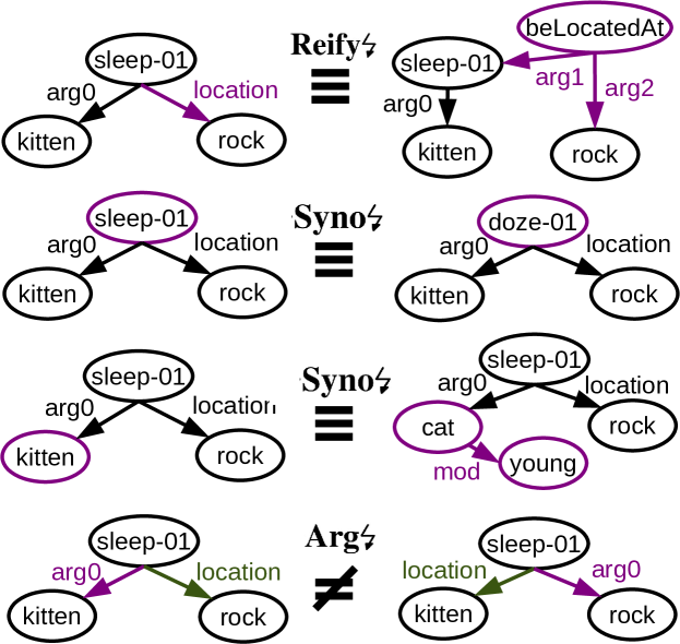
Figure 4: Examples for $f$ and $g$ graph transforms.

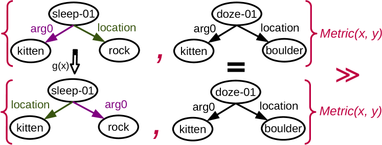
Figure 5: Metric objective example for Arg↯.

5.2 Meaning-altering graph transforms

Role confusion (Arg↯)

A naïve AMR metric could be one that treats an AMR as a bag-of-nodes, omitting structural information, such as edges and edge-labels. Such metrics could exhibit misleadingly high correlation scores with human ratings, solely due to a high overlap in concept content.

Hence, we design adversarial instances that can probe an AMR metric when confronted with cases of opposing factuality (e.g., polarity, modality or relation inverses), while concept overlap is largely preserved. We design a function

$$\mathcal{G}\neq g(\mathcal{G}),$$ (17)

that confuses role labels (see Arg↯ in Figure 4). We make use of this function to turn two paraphrastic AMRs ($\mathcal{G}$, $\mathcal{G}^{\prime}$) into non-paraphrastic AMRs, by appling $g$ to either $\mathcal{G}$, or $\mathcal{G}^{\prime}$, but not both.

In some cases $g$ may create a meaning that still makes sense (The tiger bites the snake. $\rightarrow$ The snake bites the tiger.), while in others, $g$ may induce a non-sensical meaning (The tiger jumps on the rock. $\rightarrow$ The rock jumps on the tiger.). However, this is not our primary concern, since in all cases, applying $g$ achieves our main goal: it returns a different meaning that turns a paraphrase-relation between two AMRs into a non-paraphrastic one.

To implement Arg↯, for each data set (PARA, STS, SICK) we create one new data subset. First, i) we collect all paraphrases from the initial data (in SICK and STS these are pairs with maximum human score). ii) We iterate over the AMR pairs $(\mathcal{G},\mathcal{G}^{\prime})$ and randomly select the first or second AMR from the tuple. We then collect all $n$ nodes with more than one outgoing edge. If $n=0$, we skip this AMR pair (the pair will not be contained in the data). If $n>0$, we apply the meaning altering function $g$ and randomly flip edge labels. Finally, we add the original $(\mathcal{G},\mathcal{G}^{\prime})$ to our data with the label paraphrase, and the altered pair $(\mathcal{G},g(\mathcal{G}^{\prime}))$ with the label non-paraphrase (cf. Figure 5). Per graph, we allow a maximum of 3 role confusion operations (see Table 3 for processing statistics).

5.3 Discussion

Safety of robustness objectives

We have proposed three challenging robustness objectives. Reify↯ changes the graph structure, but preserves the meaning. Arg↯ keeps the graph structure (modulo edge labels) while changing the meaning. Syno↯ changes node labels and possibly the graph structure and aims at preserving the meaning.

Reify↯ and Arg↯ are fully safe: they are well defined and are guaranteed to fulfill our goal (Eq. 12 and 17): meaning-preserving or -altering graph transforms. Syno↯ is more experimental and has (at least) three failure modes. In the first mode, depending on context, a human similarity judgments could change when near-synonyms are chosen (sleep $\rightarrow$ doze, a young cat $\rightarrow$ kitten, etc.). The second mode occurs when WSD commits an error (e.g., minister (political sense) $\rightarrow$ priest). A third mode are societal biases found in WordNet (e.g., the node girl may be mapped onto its ‘synonym’ missy). The third mode may not really be a failure, since it may not change the human rating, but, nevertheless, it may be undesirable.

In conclusion, Reify↯ and Arg↯ confusion constitute safe robustness challenges, while results on Syno↯ have to be taken with a grain of salt.

Status of the challenges in Bamboo and outlook

We believe that a key benefit of the robustness challenges lies in their potential to provide complementary performance indicators, in addition to evaluation on the Main partition of Bamboo (cf. §4). In particular, the challenges may serve to assess metrics more deeply, uncover potential weak spots, and help select among metrics, e.g., when performance differences on Main are small. In this work, however, the complementary nature of Reify↯, Syno↯ or Arg↯ versus Main is only reflected in the name of the partitions, and in our experiments, we consider all partitions equally. Future work may deviate from this setup.

Our proposed robustness challenges are also by no means exhaustive, and we believe that there is ample room for developing more challenges (extending Bamboo) or experimenting with different setups of our challenges (varying Bamboo ). For these reasons, it is possible that future work may justify alternative or enhanced setups, extensions and variations of Bamboo.

6 Experimental insights

			Main			Reify↯			Syno↯			Arg↯			amean	hmean
	speed	align	STS	SICK	PARA	STS	SICK	PARA	STS	SICK	PARA	STS	SICK	PARA	-	-
Smatch	-	✓	58.45	59.72	41.25	57.98	61.81	39.66	56.14	57.39	39.58	48.05	70.53	24.75	51.28	47.50
WSmatch	-	✓	53.06	59.24	38.64	53.39	61.17	37.49	51.41	57.56	37.85	42.47	66.79	22.68	48.48	44.58
S2match default	-	✓	56.38	58.15	42.16	55.65	60.04	40.41	56.05	57.17	40.92	46.51	70.90	26.58	50.91	47.80
S2match	-	✓	58.82	60.42	42.55	58.08	62.25	40.60	56.70	57.92	41.22	48.79	71.41	27.83	52.22	49.07
Sema	++	✗	55.90	53.32	33.43	55.51	56.16	32.33	50.16	48.87	29.11	49.73	68.18	22.79	46.29	41.85
SemBleu k=1	++	✗	66.03	62.88	39.72	61.76	62.10	38.17	61.83	58.83	37.10	1.99	1.47	1.40	41.11	5.78
SemBleu k=2	++	✗	60.62	59.86	36.88	57.68	59.64	36.24	57.34	56.18	33.26	44.54	67.54	16.60	48.87	42.13
SemBleu k=3	++	✗	56.49	57.76	32.47	54.84	57.70	33.25	52.82	53.47	28.44	49.06	69.49	24.27	47.50	42.82
SemBleu k=4	++	✗	53.19	56.69	29.61	52.28	56.12	30.11	49.31	52.11	25.56	49.75	69.58	29.44	46.15	41.75
WLK (ours)	++	✗	64.86	61.52	37.35	62.69	62.55	36.49	59.41	56.60	33.71	45.89	64.70	19.47	50.44	44.35
WWLK (ours)	+	✓	63.15	65.58	37.55	59.78	65.53	35.81	59.40	59.98	32.86	13.98	42.79	7.16	45.30	28.83
WWLKΘ (ours)	+	✓	66.94	67.64	37.91	64.34	65.49	39.23	60.11	62.29	35.15	55.03	75.06	29.64	54.90	50.26

Table 4: Bamboo benchmark result of AMR metrics. All numbers are Pearson’s $\rho\times 100$. ++: linear time complexity; +: polynomial time complexity; -: NP complete.

Questions posed to Bamboo

Bamboo allows us to address several open questions: The first set of questions aims to gain more knowledge about previously released metrics. I.a., we would like to know: What semantic aspects of AMR does a metric measure? If a metric has hyper-parameters (e.g., SemBleu), which hyper-parameters are suitable (for a specific objective)? Does the costly alignment of Smatch pay off, by yielding better predictions, or do the faster alignment-free metrics offer a ‘free-lunch’? A second set of questions aims to evaluate our proposed novel AMR similarity metrics, and to assess their potential advantages.

Experimental setup

We evaluate all metrics on the test set of Bamboo. The two hyper-parameters of S²match, that determine when concepts are similar, are set with a small search on the development set (by contrast, S²match _default denotes the default setup). WWLK_θ is trained with batch size 16 on the training data. S²match, WWLK and WWLK_θ all make use of GloVe embeddings Pennington et al. (2014).

Our main evaluation metric is Pearson’s $\rho$ between a metric’s output and the human ratings. Additionally, we consider two global performance measures to better rank AMR metrics: the arithmetic mean (amean) and the harmonic mean (hmean) over a metric’s results achieved in all tasks. Hmean is always $\leq$ $amean$ and is driven by low outliers. Hence, a large difference between amean and hmean serves as a warning light for a metric that is extremely vulnerable in a specific task.

6.1 Bamboo studies previous metrics

Table 4 shows AMR metric results on Bamboo across all three human similarity rating types (STS, SICK, PARA) and our four challenges: Main represents the standard setup (cf. §4), whereas Reify↯, Syno↯ and Arg↯ test the metric robustness (cf. §5).

Smatch and S²match rank 1^st and 2^nd of previous metrics

Smatch, our baseline metric, provides strong results across all tasks (Table 4, amean: 51.28). With default parameters, S²match_default performs slightly worse on the main data for STS and SICK, but improves upon Smatch on PARA, achieving a slight overall improvement with respect to hmean (+0.30), but not amean (-0.37). S²match is more robust against Syno↯ (e.g., +4.6 on Syno↯ STS vs. Smatch), and when confronted with reified graphs (Reify↯ STS +3.3 vs. Smatch).

Finally, S²match, after setting its two hyper-parameters with a small search on the development data, consistently improves upon Smatch over all tasks (amean: +0.94, hmean: +1.57).

WSmatch: Are nodes near the root more important?

The hypothesis underlying WSmatch is that concepts that are located near the top of an AMR have a higher impact on AMR similarity ratings. Interestingly, WSmatch mostly falls short of Smatch, offering substantially lower performance on all main tasks and all robustness checks, resulting in reduced overall amean and hmean scores (e.g., main STS: -5.39 vs. Smatch, amean: -2.8 vs. Smatch, hmean: -2.9 vs. Smatch). This contradicts the ‘core-semantics’ hypothesis and provides novel evidence that semantic concepts that influence human similarity ratings are not necessarily located close to AMR roots.

BFS-based metrics I: Sema increases speed but pays a price

Next, we find that Sema achieves lower scores in almost all categories, when compared with Smatch (amean: -4.99, hmean -5.65), ending up at rank 7 (according to hmean and amean) among prior metrics. It is similar to Smatch in that it extracts triples from graphs, but differs by not providing an alignment. Therefore, it can only loosely model some phenomena, and we conclude that the increase in speed comes at the cost of a substantial drop in modeling capacity.

BFS-based metrics II: SemBleu is fast, but is sensitive to $k$

Results for SemBleu show that it is very sensible to parameterizations of $k$. Notably, k=1, which means that the method only extracts bags of nodes, achieves strong results on SICK and STS. On PARA, however, SemBleu is outperformed by S²match, for all settings of $k$ (best $k$ (k=2): -2.8 amean, -4.7 hmean). Moreover, all variants of SemBleu are vulnerable to robustness checks. E.g., k=2, and, naturally, k=1 are easily fooled by Arg↯, where performance drops massively. k=4, on the other hand, is most robust against Arg↯, but overall it falls behind k=2.

Since SemBleu is asymmetric, we also re-compute the metric in a ‘symmetric’ way by averaging the metric result over different argument orders. We find that this can slightly increase its performance ([k, amean, hmean]: [1, +0.8, +0.6]; [2, +0.5, +0.4]; [3, +0.2, +0.2]; [4, +0.1, +0.0]).

In sum, our conclusions concerning SemBleu are: i) SemBleu _k=1 (but not SemBleu _k=3) performs well when measuring similarity and relatedness. However, SemBleu _k=1 is naïve and easily fooled (Arg↯). ii) Hence, we recommend k=2 as a good tradeoff between robustness and performance, with overall rank 4 (amean) and 6 (hmean).

6.2 Bamboo assesses novel metrics

We now discuss results of our proposed metrics based on the Weisfeiler-Leman Kernel.

Standard Weisfeiler-Leman (WLK) is fast and a strong baseline for AMR similarity

First, we visit the classic Weisfeiler-Leman kernel. Like SemBleu and Sema, the (alignment-free) method is very fast. However, it outperforms these metrics in almost all tasks (score difference against second best alignment-free metric: ([a$\mid$h]mean: +1.6, +1.5) but falls behind alignment-based Smatch ([a$\mid$h]mean: -0.8, -3.2). Specifically, WLK proves robust against Reify↯ but appears more vulnerable against Syno↯ (-5 points on STS and SICK) and Arg↯ (notably PARA, with -10 points).

The better performance, compared to SemBleu and Sema, may be due to the fact that WLK (unlike SemBleu and Sema) does not perform BFS traversal from the root, which may reduce biases.

WWLK and WWLK_θ obtain first ranks

Basic WWLK exhibits strong performance on SICK (ranking second on main and first on Reify↯). However, it has large vulnerabilities, as exposed by Arg↯, where only SemBleu _k=1 ranks lower. This can be explained by the fact that WWLK (7.2 Pearson’s $\rho$ on PARA Arg↯) only weakly considers the semantic relations (whereas SemBleu _k=1 does not consider semantic relations in the first place).

WWLK_Θ, our proposed algorithm for edge label learning, mitigates this vulnerability (29.6 Pearson’s $\rho$ on PARA Arg↯, 1^st rank). Learning edge labels also helps assessing similarity (STS) and relatedness (SICK), with substantial improvements over standard WWLK and Smatch (STS: 66.94, +3.9 vs. WWLK and +10.6 vs. Smatch; SICK +2.1 vs. WWLK and +8.4 vs. Smatch).

In sum, WWLK_θ occupies rank 1 of all considered metrics (amean and hmean), outperforming all non-alignment based metrics by large margins (amean +4.5 vs. WLK and +6.0 vs. SemBleu _k=2; hmean +5.9 vs. WLK and +8.1 vs. SemBleu _k=2), but also the alignment-based ones, albeit by lower margins (amean +2.7 vs. S²match; hmean + 1.2 vs. S²match).

6.3 Analyzing hyper-parameters of (W)WLK

	K (#WL iters)
	basic (K=2)		K=1		K=3		K=4
	amean	hmean	amean	hmean	amean	hmean	amean	hmean
WLK	50.4	44.4	49.8	44.2	47.6	42.4	46.4	41.5
WWLK	45.3	28.8	43.4	15.3	45.7	31.4	42.3	24.0
WWLKθ	54.9	50.3	52.2	35.4	55.2	51.1	50.8	47.3

Table 5: WLK variants with different K.

Setting K in (W)WLK

How does setting the number of iterations in Weisfeiler-Leman affect predictions? Table 5 shows K=2 is a good choice for all WLK variants. K=3 slightly increases performance in the latent variants (WWLK: +0.4 amean; WWLK_θ: +0.3 amean), but lowers performance for the fast symbolic matching WLK (-2.8 amean). This drop is somewhat expected: K$>$2 introduces much sparsity in the symbolic WLK feature space.

	undirected		TOP-DOWN		BOTTOM-UP		2WAYS
	amean	hmean	amean	hmean	amean	hmean	amean	hmean
WLK	50.4	44.4	50.3	44.3	50.2	43.8	49.5	41.8
WWLK	45.3	28.8	43.7	22.0	41.6	9.9	44.8	24.1
WWLKθ	54.9	50.3	53.8	46.1	50.2	18.7	55.3	51.0

Table 6: (W)WLK: message passing directions.

WL message passing direction

Even though AMR defines directional edges, for optimal similarity ratings, it was not a-priori clear in which directions the node contextualization should be restricted when attempting to model human similarity. Therefore, so far, our WLK variants have treated AMR graphs as undirected graphs ($\leftrightarrow$). In this experiment, we study three alternate scenarios: ‘TOP-DOWN’ (forward, $\rightarrow$), where information is only passed in the direction that AMR edges point at and ‘BOTTOM-UP’ (backwards, $\leftarrow$), where information is exclusively passed in the opposite direction, and 2WAY ($\leftrightarrows$), where information is passed forwards, but for every edge $edge(x,y)$ we insert an $edge^{-1}(y,x)$. 2WAY facilitates more node interactions than either TOP-DOWN or BOTTOM-UP, while preserving directional information.

Our findings in Table 6 show a clear trend: treating AMR graphs as graphs with undirected edges offers better results than TOP-DOWN (e.g., WWLK -1.6 amean; -6.6 hmean) and considerably better results when compared to WLK in BOTTOM-UP mode (e.g., WWLK -3.7 amean; -18.9 hmean). Overall, 2WAY behaves similarly to the standard setup, with a slight improvement for WWLK_θ. Notably, the symbolic WLK variant, that does not use word embeddings, appears more robust in this experiment and differences between the three directional setups are small.

6.4 Revisiting the data quality in Bamboo

Initial quality analyses (§4) suggested that the quality of Bamboo is high, with a large proportion of AMR graphs that are of gold or silver quality. In this experiment, we study how metric rankings and predictions could change when confronted with AMRs corrected by humans. From every data set, we randomly sample 50 AMR graph pairs (300 AMRs in total). In each AMR, the human annotator searched for mistakes, and corrected them.

	STS		SICK		PARA		AVERAGE
	MHA	IMA	MHA	IMA	MHA	IMA	MHA	IMA
SM	[71, 73]	97.9	[66, 66]	99.9	[44, 44]	97.9	[60, 61]	98.6
WSM	[64, 65]	99.2	[67, 67]	99.8	[47, 49]	98.7	[59, 60]	99.2
S2Mdef	[69, 70]	97.7	[62, 63]	99.3	[44, 47]	97.7	[58, 60]	98.2
S2M	[71, 73]	97.8	[69, 70]	98.6	[41, 46]	98.0	[60, 63]	98.1
SE	[66, 66]	97.7	[55, 55]	100	[42, 46]	99.0	[55, 56]	98.9
SB2	[68, 68]	97.2	[62, 62]	99.8	[41, 42]	98.8	[57, 58]	98.6
SB3	[66, 66]	98.4	[63, 63]	99.7	[33, 34]	99.3	[54, 54]	99.1
WLK	[72, 72]	98.2	[65, 65]	99.8	[43, 46]	97.9	[60, 61]	98.6
WWLK	[77, 78]	97.8	[65, 67]	98.1	[42, 46]	97.8	[61, 63]	97.9
WWLKθ	[78, 78]	96.8	[67, 68]	98.1	[48, 48]	96.7	[64, 65]	97.2

Table 7: Retrospective sub-sample quality analysis of Bamboo graph quality and sensitivity of metrics. All values are Pearson’s $\rho\times 100$. Metric Human Agreement (MHA): $[x,y]$, where $x$ is the correlation (to human ratings) when the metric is executed on the uncorrected sample and $y$ is the same assessment on the manually post-processed sample.

We study two settings. i) Intra metric agreement (IMA): For every metric, we calculate the correlation of its predictions for the initial graph pairs versus the predictions for the graph pairs that are ensured to be correct. Note that, on one hand, a high IMA for all metrics would further corroborate the trustworthiness of Bamboo results. However, on the other hand, a high IMA for a single metric cannot be interpreted as a marker for this metric’s quality. I.e., a maximum IMA (1.0) could also indicate that a metric is completely insensitive to the human corrections. Furthermore, we study ii) Metric human agreement (MHA): Here, we correlate the metric scores against human ratings, once when fed the fully gold-ensured graph pairs and once when fed the standard graph pairs. Both measures, IMA, and IAA, can provide us with an indicator of how much metric ratings would change if Bamboo would be fully human corrected.

Results are shown in Table 7. All metrics exhibit high IMA, suggesting that potential changes in their ratings, when fed gold-ensured graphs, are quite small. Furthermore, on average, all metrics tend to exhibit slightly better correlation with the human when computed on the gold-ensured graph pairs. However, supporting the assessment of IMA, the increments in MHA appear small, ranging from a minimum increment of +0.3 (SemBleu) to a maximum increment of +2.8 (S²match), whereas WWLK yields an increment of +1.8. Generally, while this assessment has to be taken with a grain of salt due to the small sample size, it overall supports the validity of Bamboo results.

6.5 Discussion

Align or not align?

We can group metrics for graph-based meaning representations into whether they compute an alignment between AMRs or not Liu et al. (2020). A computed alignment, as in Smatch, has the advantage that it lets us assess finer-grained AMR graph similarities and divergences, by creating and exploiting a mapping that shows which specific substructures of two graphs are more or less similar to each other. On the other hand, it was still an open question whether such an alignment is worth its computational cost and enhances similarity judgments.

Experiments on Bamboo provide novel evidence on this matter: alignment-based metrics may be preferred for better accuracy. Non-alignment based metrics may be preferred if speed matters most. The latter situation may occur, e.g., when AMR metrics must be executed over a large cross-product of parses (for instance, to semantically cluster sentences from a corpus). For a balanced approach, WWLK_Θ offers a good trade-off: polynomial-time alignment and high accuracy.

Example discussion I: Wasserstein transportation analysis explains disagreement

Fig. 6 (top) shows an example where the human-assigned similarity score is relatively low (rank 1164 of 1379). Due to the graphs having the same structure ($x~{}arg0~{}y;~{}x~{}arg1~{}z$), the previous metrics (except Sema) tend to assign similarities that are relatively too high. In particular, S²match finds the exact same alignments in this case, but cannot assess the concept-relations more deeply. WWLK yields more informative alignments since they explain its decision to assign a more appropriate lower rank (1253 of 1379): substantial work is needed to transport, e.g., carry-01 to slice-01.

Example discussion II: the value of n:m alignments

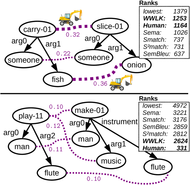
Figure 6: WWLK alignments and metric scores for dissimilar (top, STS) and similar (bottom, SICK) AMRs. Excavators indicate heavy Wasserstein work $flow\cdot cost$.

Fig. 6 (bottom) shows that WWLK produces valuable n:m alignments (play-11 vs. make-01 and music), which are needed to properly reflect similarity (note that Smatch, WSmatch and S²match only provide 1-1 alignments). Yet, the example also shows that there is still a way to go. While humans assess this near-equivalence easily, providing a relatively high score (rank 331 of 4972), all metrics considered in this paper, including ours, assign relative ranks that are too low (WWLK: 2624). Future work may incorporate external PropBank Palmer et al. (2005) knowledge into AMR metrics. In PropBank, sense 11 of play is defined as equivalent to making music.

7 Conclusion

Our contributions in this work are three-fold: i) We propose a suite of novel Weisfeiler-Leman AMR similarity metrics that are able to reconcile a performance conflict between precision of AMR similarity ratings and the efficiency of computing alignments. ii) We release Bamboo, the first benchmark that allows researchers to assess AMR metrics empirically, setting the stage for future work on graph-based meaning representation metrics. iii) We showcase the utility of Bamboo, by applying it to profile existing AMR metrics, uncovering hitherto unknown strengths or weaknesses, and to assess the strengths of our newly proposed metrics that we derive and further develop from the classic Weisfeiler-Leman Kernel. We show that through Bamboo we are able to gain novel insight regarding suitable hyperparameters of different metric types, and to gain novel perspectives on how to further improve AMR similarity metrics to achieve better correlation with the degree of meaning similarity of paired sentences, as perceived by humans.

References

- Anchiêta et al. (2019) Rafael Torres Anchiêta, Marco Antonio Sobrevilla Cabezudo, and Thiago Alexandre Salgueiro Pardo. 2019. Sema: an extended semantic evaluation for amr. In (To appear) Proceedings of the 20th Computational Linguistics and Intelligent Text Processing. Springer International Publishg.
- Banarescu et al. (2013) Laura Banarescu, Claire Bonial, Shu Cai, Madalina Georgescu, Kira Griffitt, Ulf Hermjakob, Kevin Knight, Philipp Koehn, Martha Palmer, and Nathan Schneider. 2013. Abstract meaning representation for sembanking. In Proceedings of the 7th Linguistic Annotation Workshop and Interoperability with Discourse, pages 178–186, Sofia, Bulgaria. Association for Computational Linguistics.
- Banerjee and Pedersen (2002) Satanjeev Banerjee and Ted Pedersen. 2002. An adapted lesk algorithm for word sense disambiguation using wordnet. In International conference on intelligent text processing and computational linguistics, pages 136–145. Springer.
- Baudiš et al. (2016a) Petr Baudiš, Jan Pichl, Tomáš Vyskočil, and Jan Šedivỳ. 2016a. Sentence pair scoring: Towards unified framework for text comprehension. arXiv preprint arXiv:1603.06127.
- Baudiš et al. (2016b) Petr Baudiš, Silvestr Stanko, and Jan Šedivý. 2016b. Joint learning of sentence embeddings for relevance and entailment. In Proceedings of the 1st Workshop on Representation Learning for NLP, pages 8–17, Berlin, Germany. Association for Computational Linguistics.
- Blloshmi et al. (2020) Rexhina Blloshmi, Rocco Tripodi, and Roberto Navigli. 2020. XL-AMR: Enabling cross-lingual AMR parsing with transfer learning techniques. In Proceedings of the 2020 Conference on Empirical Methods in Natural Language Processing (EMNLP), pages 2487–2500, Online. Association for Computational Linguistics.
- Bonial et al. (2020) Claire Bonial, Stephanie M. Lukin, David Doughty, Steven Hill, and Clare Voss. 2020. InfoForager: Leveraging semantic search with AMR for COVID-19 research. In Proceedings of the Second International Workshop on Designing Meaning Representations, pages 67–77, Barcelona Spain (online). Association for Computational Linguistics.
- Budanitsky and Hirst (2006) Alexander Budanitsky and Graeme Hirst. 2006. Evaluating wordnet-based measures of lexical semantic relatedness. Computational linguistics, 32(1):13–47.
- Cai and Lam (2019) Deng Cai and Wai Lam. 2019. Core semantic first: A top-down approach for AMR parsing. In Proceedings of the 2019 Conference on Empirical Methods in Natural Language Processing and the 9th International Joint Conference on Natural Language Processing (EMNLP-IJCNLP), pages 3799–3809, Hong Kong, China. Association for Computational Linguistics.
- Cai and Knight (2013) Shu Cai and Kevin Knight. 2013. Smatch: an evaluation metric for semantic feature structures. In Proceedings of the 51st Annual Meeting of the Association for Computational Linguistics (Volume 2: Short Papers), pages 748–752, Sofia, Bulgaria. Association for Computational Linguistics.
- Cer et al. (2017) Daniel Cer, Mona Diab, Eneko Agirre, Iñigo Lopez-Gazpio, and Lucia Specia. 2017. SemEval-2017 task 1: Semantic textual similarity multilingual and crosslingual focused evaluation. In Proceedings of the 11th International Workshop on Semantic Evaluation (SemEval-2017), pages 1–14, Vancouver, Canada. Association for Computational Linguistics.
- Conn et al. (2009) Andrew R Conn, Katya Scheinberg, and Luis N Vicente. 2009. Introduction to derivative-free optimization. SIAM.
- Dolan and Brockett (2005) William B. Dolan and Chris Brockett. 2005. Automatically constructing a corpus of sentential paraphrases. In Proceedings of the Third International Workshop on Paraphrasing (IWP2005).
- Gardent et al. (2017) Claire Gardent, Anastasia Shimorina, Shashi Narayan, and Laura Perez-Beltrachini. 2017. The WebNLG challenge: Generating text from RDF data. In Proceedings of the 10th International Conference on Natural Language Generation, pages 124–133, Santiago de Compostela, Spain. Association for Computational Linguistics.
- Gehrmann et al. (2021) Sebastian Gehrmann, Tosin Adewumi, Karmanya Aggarwal, Pawan Sasanka Ammanamanchi, Aremu Anuoluwapo, Antoine Bosselut, Khyathi Raghavi Chandu, Miruna Clinciu, Dipanjan Das, Kaustubh D Dhole, et al. 2021. The gem benchmark: Natural language generation, its evaluation and metrics. arXiv preprint arXiv:2102.01672.
- Goodman (2020) Michael Wayne Goodman. 2020. Penman: An open-source library and tool for AMR graphs. In Proceedings of the 58th Annual Meeting of the Association for Computational Linguistics: System Demonstrations, pages 312–319, Online. Association for Computational Linguistics.
- Hofmann et al. (2008) Thomas Hofmann, Bernhard Schölkopf, and Alexander J Smola. 2008. Kernel methods in machine learning. The annals of statistics, pages 1171–1220.
- Kapanipathi et al. (2021) Pavan Kapanipathi, Ibrahim Abdelaziz, Srinivas Ravishankar, Salim Roukos, Alexander Gray, Ramon Astudillo, Maria Chang, Cristina Cornelio, Saswati Dana, Achille Fokoue, et al. 2021. Leveraging abstract meaning representation for knowledge base question answering. Findings of the Association for Computational Linguistics: ACL.
- Kiefer et al. (1952) Jack Kiefer, Jacob Wolfowitz, et al. 1952. Stochastic estimation of the maximum of a regression function. The Annals of Mathematical Statistics, 23(3):462–466.
- Kolb (2009) Peter Kolb. 2009. Experiments on the difference between semantic similarity and relatedness. In Proceedings of the 17th Nordic Conference of Computational Linguistics (NODALIDA 2009), pages 81–88, Odense, Denmark. Northern European Association for Language Technology (NEALT).
- Lesk (1986) Michael Lesk. 1986. Automatic sense disambiguation using machine readable dictionaries: how to tell a pine cone from an ice cream cone. In Proceedings of the 5th annual international conference on Systems documentation, pages 24–26.
- Liu et al. (2020) Jiangming Liu, Shay B. Cohen, and Mirella Lapata. 2020. Dscorer: A fast evaluation metric for discourse representation structure parsing. In Proceedings of the 58th Annual Meeting of the Association for Computational Linguistics, pages 4547–4554, Online. Association for Computational Linguistics.
- Lyu and Titov (2018) Chunchuan Lyu and Ivan Titov. 2018. AMR parsing as graph prediction with latent alignment. In Proceedings of the 56th Annual Meeting of the Association for Computational Linguistics (Volume 1: Long Papers), pages 397–407, Melbourne, Australia. Association for Computational Linguistics.
- Ma et al. (2019) Qingsong Ma, Johnny Wei, Ondřej Bojar, and Yvette Graham. 2019. Results of the WMT19 metrics shared task: Segment-level and strong MT systems pose big challenges. In Proceedings of the Fourth Conference on Machine Translation (Volume 2: Shared Task Papers, Day 1), pages 62–90, Florence, Italy. Association for Computational Linguistics.
- Marelli et al. (2014) Marco Marelli, Stefano Menini, Marco Baroni, Luisa Bentivogli, Raffaella Bernardi, and Roberto Zamparelli. 2014. A SICK cure for the evaluation of compositional distributional semantic models. In Proceedings of the Ninth International Conference on Language Resources and Evaluation (LREC-2014), pages 216–223, Reykjavik, Iceland. European Languages Resources Association (ELRA).
- May (2016) Jonathan May. 2016. Semeval-2016 task 8: Meaning representation parsing. In Proceedings of the 10th international workshop on semantic evaluation (semeval-2016), pages 1063–1073.
- May and Priyadarshi (2017) Jonathan May and Jay Priyadarshi. 2017. Semeval-2017 task 9: Abstract meaning representation parsing and generation. In Proceedings of the 11th International Workshop on Semantic Evaluation (SemEval-2017), pages 536–545.
- Naseem et al. (2019) Tahira Naseem, Abhishek Shah, Hui Wan, Radu Florian, Salim Roukos, and Miguel Ballesteros. 2019. Rewarding Smatch: Transition-based AMR parsing with reinforcement learning. In Proceedings of the 57th Annual Meeting of the Association for Computational Linguistics, pages 4586–4592, Florence, Italy. Association for Computational Linguistics.
- van Noord et al. (2018) Rik van Noord, Lasha Abzianidze, Hessel Haagsma, and Johan Bos. 2018. Evaluating scoped meaning representations. In Proceedings of the Eleventh International Conference on Language Resources and Evaluation (LREC-2018), Miyazaki, Japan. European Languages Resources Association (ELRA).
- Oepen et al. (2020) Stephan Oepen, Omri Abend, Lasha Abzianidze, Johan Bos, Jan Hajic, Daniel Hershcovich, Bin Li, Tim O’Gorman, Nianwen Xue, and Daniel Zeman. 2020. Mrp 2020: The second shared task on cross-framework and cross-lingual meaning representation parsing. In Proceedings of the CoNLL 2020 Shared Task: Cross-Framework Meaning Representation Parsing, pages 1–22.
- Opitz (2020) Juri Opitz. 2020. AMR quality rating with a lightweight CNN. In Proceedings of the 1st Conference of the Asia-Pacific Chapter of the Association for Computational Linguistics and the 10th International Joint Conference on Natural Language Processing, pages 235–247, Suzhou, China. Association for Computational Linguistics.
- Opitz and Frank (2021) Juri Opitz and Anette Frank. 2021. Towards a decomposable metric for explainable evaluation of text generation from AMR. In Proceedings of the 16th Conference of the European Chapter of the Association for Computational Linguistics: Main Volume, pages 1504–1518, Online. Association for Computational Linguistics.
- Opitz et al. (2020) Juri Opitz, Letitia Parcalabescu, and Anette Frank. 2020. Amr similarity metrics from principles. Transactions of the Association for Computational Linguistics, 8:522–538.
- Palmer et al. (2005) Martha Palmer, Daniel Gildea, and Paul Kingsbury. 2005. The proposition bank: An annotated corpus of semantic roles. Computational Linguistics, 31(1):71–106.
- Papineni et al. (2002) Kishore Papineni, Salim Roukos, Todd Ward, and Wei-Jing Zhu. 2002. Bleu: a method for automatic evaluation of machine translation. In Proceedings of the 40th Annual Meeting of the Association for Computational Linguistics, pages 311–318, Philadelphia, Pennsylvania, USA. Association for Computational Linguistics.
- Pedersen (2007) Ted Pedersen. 2007. Unsupervised corpus-based methods for wsd. Word sense disambiguation, pages 133–166.
- Pennington et al. (2014) Jeffrey Pennington, Richard Socher, and Christopher Manning. 2014. Glove: Global vectors for word representation. In Proceedings of the 2014 Conference on Empirical Methods in Natural Language Processing (EMNLP), pages 1532–1543, Doha, Qatar. Association for Computational Linguistics.
- Raffel et al. (2019) Colin Raffel, Noam Shazeer, Adam Roberts, Katherine Lee, Sharan Narang, Michael Matena, Yanqi Zhou, Wei Li, and Peter J. Liu. 2019. Exploring the limits of transfer learning with a unified text-to-text transformer. CoRR, abs/1910.10683.
- Shervashidze et al. (2011) Nino Shervashidze, Pascal Schweitzer, Erik Jan Van Leeuwen, Kurt Mehlhorn, and Karsten M Borgwardt. 2011. Weisfeiler-lehman graph kernels. Journal of Machine Learning Research, 12(9).
- Sheth et al. (2021) Janaki Sheth, Young-Suk Lee, Ramon Fernandez Astudillo, Tahira Naseem, Radu Florian, Salim Roukos, and Todd Ward. 2021. Bootstrapping Multilingual AMR with Contextual Word Alignments. arXiv preprint arXiv:2102.02189.
- Song and Gildea (2019) Linfeng Song and Daniel Gildea. 2019. SemBleu: A robust metric for AMR parsing evaluation. In Proceedings of the 57th Annual Meeting of the Association for Computational Linguistics, pages 4547–4552, Florence, Italy. Association for Computational Linguistics.
- Spall (1987) James C Spall. 1987. A stochastic approximation technique for generating maximum likelihood parameter estimates. In 1987 American control conference, pages 1161–1167. IEEE.
- Spall (1998) James C Spall. 1998. An overview of the simultaneous perturbation method for efficient optimization. Johns Hopkins apl technical digest, 19(4):482–492.
- Togninalli et al. (2019) Matteo Togninalli, Elisabetta Ghisu, Felipe Llinares-López, Bastian Rieck, and Karsten Borgwardt. 2019. Wasserstein weisfeiler-lehman graph kernels. In Advances in Neural Information Processing Systems, volume 32, pages 6436–6446. Curran Associates, Inc.
- Uhrig et al. (2021) Sarah Uhrig, Yoalli Garcia, Juri Opitz, and Anette Frank. 2021. Translate, then parse! a strong baseline for cross-lingual AMR parsing. In Proceedings of the 17th International Conference on Parsing Technologies and the IWPT 2021 Shared Task on Parsing into Enhanced Universal Dependencies (IWPT 2021), pages 58–64, Online. Association for Computational Linguistics.
- Wang (2020) Chen Wang. 2020. An overview of spsa: recent development and applications. arXiv preprint arXiv:2012.06952.
- Weisfeiler and Leman (1968) Boris Weisfeiler and Andrei Leman. 1968. The reduction of a graph to canonical form and the algebra which appears therein. NTI, Series, 2(9):12–16.
- Xu et al. (2020) Dongqin Xu, Junhui Li, Muhua Zhu, Min Zhang, and Guodong Zhou. 2020. Improving AMR parsing with sequence-to-sequence pre-training. In Proceedings of the 2020 Conference on Empirical Methods in Natural Language Processing (EMNLP), pages 2501–2511, Online. Association for Computational Linguistics.
- Yanardag and Vishwanathan (2015) Pinar Yanardag and SVN Vishwanathan. 2015. Deep graph kernels. In Proceedings of the 21th ACM SIGKDD International Conference on Knowledge Discovery and Data Mining, pages 1365–1374.
- Zhang et al. (2018) Sheng Zhang, Xutai Ma, Rachel Rudinger, Kevin Duh, and Benjamin Van Durme. 2018. Cross-lingual decompositional semantic parsing. In Proceedings of the 2018 Conference on Empirical Methods in Natural Language Processing, pages 1664–1675, Brussels, Belgium. Association for Computational Linguistics.
- Zhu et al. (2018) Yaoming Zhu, Sidi Lu, Lei Zheng, Jiaxian Guo, Weinan Zhang, Jun Wang, and Yong Yu. 2018. Texygen: A benchmarking platform for text generation models. In The 41st International ACM SIGIR Conference on Research & Development in Information Retrieval, pages 1097–1100.