Waiting-times statistics in boundary driven free fermion chains

Abstract

We study the waiting-time distributions (WTDs) of quantum chains coupled to two Lindblad baths at each end. Our focus is on free fermion chains, where we derive closed-form expressions in terms of single-particle matrices, allowing one to study arbitrarily large chain sizes. In doing so, we also derive formulas for 2-point correlation functions involving non-Hermitian propagators.

I Introduction

Transport in quantum chains constitutes a major research direction in non-equilibrium physics. The interplay between quantum coherent interactions and dissipative elements is known to produce a wide variety of physical phenomena. The basic example is the tuning of the ensuing transport regimes (e.g. ballistic, diffusive, etc.), which can be accomplished e.g. by modifying the internal system interaction Bertini2020; Znidaric2011; Landi2015a; Gopalakrishnan2019; Bulchandani2019; Ilievski2018. Further tuning the dissipation can also lead to noise-enhanced transport Viciani2015; Plenio2008; Biggerstaff2016; Maier2019; DeLeon-Montiel2015; Dwiputra2020. These developments open the prospect for numerous potential applications, such as quantum thermoelectricity Benenti2017a; Mahan1996; Yamamoto2015a; Dubi2011; Whitney2014 and thermal rectifiers Li2012; Pereira2013a; Werlang2014; Avila2013; Schuab2016a; Balachandran2018; Pereira2010b; Pereira2010; Wang2007; Hu2006; Landi2014b; Silva2020; Chioquetta2021.

As far as transport is concerned, most studies in quantum chains focus on either one of two scenarios Bertini2020. The first is unitary time evolution, where the system is prepared in a localized wave-packet and is then allowed to evolve unitarily. And the second is the steady-state that is obtained when the system is placed in contact with two baths at different temperatures and/or chemical potentials. This is further divided into systems described in terms of coherent transport, e.g. the Landauer-Büttiker formalism Datta1997a; Benenti2017a, or systems described in terms of a quantum master equation, often referred to as boundary-driven systems Landi2021.

In the case of steady-states, even though the density matrix is no longer changing in time, the underlying process is still stochastic: At any given time, an excitation may enter from one of the baths and then travel through the system (possibly interacting with other excitations) until it eventually leaves to either bath. The quantum nature of the system makes this description much richer, as interference effects abound. But if one only looks at the steady-state density matrix, these effects are completely ignored.

The problem can be viewed pictorially as a detector with four colors, representing an excitation entering/leaving the left/right baths (Fig. 1). Each time an event occurs, a certain color clicks. The complete statistics of the detection events, including the times between clicks, as well as the colors of the clicks, is captured by the theory of Full Counting Statistics (FCS) Levitov1993; Esposito2007; Esposito2009; Brandes2008. The toolbox of FCS is extremely powerful, but usually difficult to apply, specially on many-body systems. For this reason, most practical studies on FCS have focused on the long-time statistics; i.e., on the accumulated number of clicks after a very long time, which satisfies a large-deviation principle Touchette2009; Touchette2012.

A particularly interesting aspect of FCS concerns the waiting time distribution (WTD) between successive clicks Cohen-Tannoudji1986; Plenio1998a. There has been significant work on the study of WTDs in coherent conductors Brandes2008; Schaller2009; Albert2011; Albert2012; Rajabi2013; Thomas2013; Thomas2014; Haack2014; Dasenbrook2015; Ptaszynski2017a; Ptaszynski2017; Stegmann2021; Stegmann2018, such as double quantum dots or point contacts. However, WTDs are also useful in many other problems, where they have not yet been thoroughly explored. This manuscript will be concerned with boundary driven systems, comprised of a one-dimensional quantum chain coupled to two baths at each end, as described by a Lindblad master equation. The theory of WTDs in this case was laid down in Brandes2008, and subsequently applied to double quantum dot systems Schaller2009; Ptaszynski2017a, Cooper pair splitters Walldorf2018 and synchronized charge oscillations Kleinherbers2021.

Here we develop formulas for the waiting-time distribution of free fermion chain. As with most non-interacting problems, this allows the WTD to be written in terms of matrix elements and determinants of $L\times L$ matrices (where $L$ is the number of sites in the chain), hence allowing one to study chains of arbitrary size. Despite being a non-interacting problem, the analysis turns out to be non-trivial since the time evolution between quantum jumps is non-Hermitian Wiseman2009. For this reason, we proceed by first casting the WTDs in terms of 2-point correlation functions involving non-Hermitian unitary evolution operators. We then develop general formulas for such propagators, which could find use beyond the present context. As an application, we study a simple tight-binding chain.

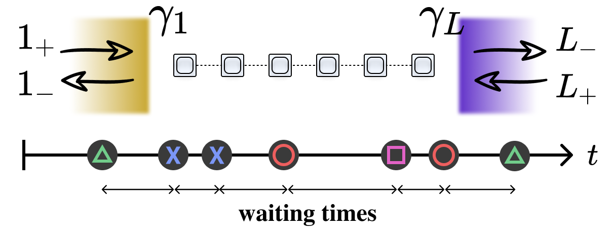
Figure 1: Top: A quantum chain of length $L$, with four possible dissipation channels, associated to the injection/extraction of an excitation at the first/last sites, with coupling strengths $\gamma_{1(L)}$. Bottom: the interest in this work is on the waiting time distribution between clicks in each channel (here represented by buttons of a video game controller).

II Formal framework

We consider a one-dimensional fermionic chain with $L$ sites, each represented by an annihilation operator $c_{i}$. The system Hamiltonian is assumed to be quadratic, of the form

$$H=\sum\limits_{i,j}h_{ij}c_{i}^{\dagger}c_{j},$$ (1)

with a coefficient matrix $h$. The WTDs of free fermion chains were studied in Thomas2014, but only in the case of unitary dynamics. Instead, here we assume the system evolves connected to two local baths, coupled at sites 1 and $L$, and kept at Fermi-Dirac distributions $f_{1}$ and $f_{L}$. The dynamics is thus assumed to be governed by the local master equation

$$\frac{d\rho}{dt}=\mathcal{L}(\rho)=-i[H,\rho]+\sum\limits_{i=1,L}\Big{\{}\gamma_{i}^{-}D[c_{i}]+\gamma_{i}^{+}D[c_{i}^{\dagger}]\Big{\}},$$ (2)

where $\gamma_{i}^{-}=\gamma_{i}(1-f_{i})$ and $\gamma_{i}^{+}=\gamma_{i}f_{i}$, with $\gamma_{i}$ being the coupling strengths to each bath. Here $D[A]=A\rho A^{\dagger}-\frac{1}{2}\{A^{\dagger}A,\rho\}$ is a Lindblad dissipator with arbitrary operator $A$.

The WTD in this case is defined in the context of Full Counting Statistics. We split the Liouvillian in Eq. (2) as

$$\mathcal{L}=\mathcal{L}_{0}+\sum\limits_{k}\mathcal{J}_{k},$$ (3)

where $\mathcal{J}_{k}$ represent the four possible jump channels (“four colors in the detector”), which we label as $1_{-}$, $1_{+}$, $L_{-}$, $L_{+}$: rCCCCCL J_1_-(ρ) &= γ_1^- c_1 ρc_1^†   J_1_+(ρ) = γ_1^+ c_1^†ρc_1

J_L_-(ρ) = γ_L^- c_L ρc_L^†   J_L_+(ρ) = γ_L^+ c_L^†ρc_L For instance, channel $L_{-}$ means an excitation was absorbed by the right bath (at site $L$), and so on.

Starting from an arbitrary state $\rho$, the WTD between a jump in channel $q$ at time $0$ and a jump in channel $k$ at time $t$ is then given by Brandes2008:

$$P(t,k|q)=\frac{\mathrm{tr}\leavevmode\nobreak\ \mathcal{J}_{k}e^{\mathcal{L}_{0}t}\mathcal{J}_{q}(\rho)}{\mathrm{tr}\leavevmode\nobreak\ \mathcal{J}_{q}(\rho)},$$ (4)

which is normalized as

$$\sum\limits_{k}\int\limits_{0}^{\infty}P(t,k|q)dt=1,\qquad\forall q.$$ (5)

Eq. (4) is a (conditional) joint distribution representing both the time between clicks, as well as the channel of the click (note that clicks from different channels are usually statistically correlated Dasenbrook2015).

The marginal probability that jump $q$ is followed by jump $k$, irrespective of when it occurs, is

$$p(k|q)=\int\limits_{0}^{\infty}P(t,k|q)\leavevmode\nobreak\ dt.$$ (6)

We can also filter the WTD to consider only the statistics conditioned on the sequence of jumps being $q\to k$. From Bayes’s rule one has:

$$P(t|k,q)=P(t,k|q)/p(k|q),$$ (7)

This is now a properly normalized WTD, and so is more suitable for computing expectation values. We denote by $T$ the random waiting time between any two events. The average $E(T|k,q)$, conditioned on the sequence of channels $q\to k$, is

$$E(T|k,q)=\int\limits_{0}^{\infty}\leavevmode\nobreak\ t\leavevmode\nobreak\ P(t|k,q)\leavevmode\nobreak\ dt.$$ (8)

Similarly, the variance of the waiting time reads

$${\rm var}(T|k,q)=E(T^{2}|k,q)-E(T|k,q)^{2},$$ (9)

where $E(T^{2}|k,q)$ is defined similarly as $E(T|k,q)$.

We call attention to the fact that the WTDs defined above assume that all four channels are constantly being monitored (called “exclusive” WTDs in Walldorf2018). One could also study a situation where only channel $k$ is being monitored (“inclusive” WTD). Unfortunately, this is not related to (4) in a simple way, since the inclusive distribution must account for all possible jumps to the other channels before a click in $k$ is detected.

The WTD (4) refers to specific channels $q\to k$. One may also be interested in what shall be referred to as the net activity time distribution (NATD), which is the WTD between any two events, irrespective of the channel. In the steady-state, it can be defined as

$$P(t)=\sum\limits_{k,q}P(t,k|q)p(q),$$ (10)

where $p(q)$ is the relative frequency of occurrence for a jump of type $q$ (in the steady-state) and is given, up to a normalization, by $p(q)=\mathrm{tr}\mathcal{J}_{q}\rho$. Expectation values for NATDs may be defined similarly to e.g. Eqs. (8) and (9), and will be denoted by $E(T)$, ${\rm var}(T)$, etc.

Computing the waiting time distribution is generally hard, as it involves studying the evolution under the map $\mathcal{L}_{0}$, which is generally not completely positive and trace preserving. In fact, $\mathcal{L}_{0}$ can be decomposed as $\mathcal{L}_{0}=-i(H_{e}\rho-\rho H_{e}^{\dagger})$, where rCL H_e &= H - i2 [ γ_1 (1-f_1) c_1^†c_1 + γ_1 f_1 c_1 c_1^†,
  + γ_L (1-f_L) c_L^†c_L + γ_L f_L c_L c_L^†]. Hence, the action of $\mathcal{L}_{0}$ is tantamount to a non-Hermitian Hamiltonian evolution. Given the four possible channels in Eq. (II), there can be in total 16 WTDs (4). They can be more compactly written as rCl P(t, i_-— j_+) &= γi-⟨cjcj†⟩ tr{ c_i^†c_i e^-i H_e t c_j^†ρc_j e^i H_e^†t},
P(t, i_+— j_+) = γi+⟨cjcj†⟩ tr{ c_i c_i^†e^-i H_e t c_j^†ρc_j e^i H_e^†t},
P(t, i_-— j_-) = γi-⟨cj†cj⟩ tr{ c_i^†c_i e^-i H_e t c_j ρc_j^†e^i H_e^†t},
P(t, i_+— j_-) = γi+⟨cj†cj⟩ tr{ c_i c_i^†e^-i H_e t c_j ρc