Librational KAM tori in the secular dynamics of the $\upsilon$ Andromedæ planetary system

Abstract

We study the planetary system of $\upsilon$ Andromedæ, considering the three-body problem formed by the central star and the two largest planets, $\upsilon$ And c and $\upsilon$ And d. We adopt a secular, three-dimensional model and initial conditions within the range of the observed values. The numerical integrations highlight that the system is orbiting around a one-dimensional elliptic torus (i.e., a periodic orbit that is linearly stable). This invariant object is used as a seed for an algorithm based on a sequence of canonical transformations. The algorithm determines the normal form related to a KAM torus, whose shape is in excellent agreement with the orbits of the secular model. We rigorously prove that the algorithm constructing the final KAM invariant torus is convergent, by adopting a suitable technique based on a computer-assisted proof.

1 Introduction

The discovery of the first multiple-planet extrasolar system dates back to the very end of the last century (see [3]). Through the radial velocity method, three planets were found orbiting around one of the two stars of the binary system $\upsilon$ Andromedæ. Since then thousands of exoplanets have been observed, and among the plethora of new extrasolar planetary systems around $780$ of them host two or more planets. Of all the different detection techniques available at present day, the radial velocity method better highlights the skeleton of a multi-planetary system, as it is particularly sensitive to more massive bodies. The dynamical characteristics of radial-velocity-detected systems can strongly differ from those of the solar system. For instance, the orbits can be far more eccentric and the planets can present masses several times larger than the one of Jupiter. A proper understanding of the architecture of these systems is complicated even more by the fact that some of their orbital parameters are unknown. Concerning the radial velocity method, this applies in particular to the orbital inclination $i_{P}\,$ of an exoplanet with respect to the line of sight (see, e.g., [2]). This implies that only minimal masses for the planets can be inferred (i.e., $m_{P}\sin i_{P}$), whereas their actual values remain unknown.

In several cases, exoplanets can be observed by only one detection technique. Therefore, it is a rare occurrence that two different detection methods can be used on the same system. The planetary system of $\upsilon$ Andromedæ is then particularly interesting because it was thoroughly observed by means of both radial velocity and astrometry. This makes $\upsilon$ Andromedæ one of the most well-known and studied exoplanetary systems. Thanks to the joint observations, it was possible to determine ranges of values for the orbital inclinations of the two planets with the largest minimal masses, $\upsilon$ And c and $\upsilon$ And d (see [28]). Therefore, ranges of possible values for both planetary masses have been inferred as well. These new constraints modify substantially the study of the stability of the system. In fact, since the orbital plane of $\upsilon$ And c is highly inclined with respect to the line of sight, the actual value of the mass could be larger than $5$ times the minimal one. The same effect has a weaker impact on the determination of $\upsilon$ And d’s mass, being the increasing factor about $2.5\,$. The two-dimensional models of the $\upsilon$ Andromedæ system that were studied mainly in the first decade of this century used the minimal values of the masses. Therefore, the perturbation of the Keplerian orbits (that is due to the mutual gravitation) when considering the updated values is expected to be one order of magnitude larger. Moreover, the mutual inclination between $\upsilon$ And c and $\upsilon$ And d is quite remarkable, being about $30^{\circ}$. Taking into account that also their eccentricities are about 5 times larger than those we observe in our Jovian planets, it is natural to expect that the excursions of the secular variables can be very relevant, with a possibly dramatic impact on the stability of the system. This is confirmed by the fact that, according to the analysis described in [10], the orbits starting from many initial conditions within the range of observed values are evidently unstable. Therefore, the stability of the $\upsilon$ Andromedæ planetary system in a genuine 3D-model cannot be ensured by simply applying the AMD general criterion (see [22], where this method was introduced).

This paper aims to study the stability of the $\upsilon$ Andromedæ system in the refined framework of the KAM theory (see [19], [33] and [1]). Our approach is definitely challenging from a computational point of view, but we will show that it is able to construct tori that are invariant with respect to the secular model of the planetary Hamiltonian. In order to adapt our KAM-tori-constructing method as it has already been applied to other problems in Celestial Mechanics (see, e.g., [26] and [13]) to this particular context, a sequence of canonical transformations must be performed as a preparatory step. In particular, we will stress the key role that is played in our approach by the preliminary construction of the normal form of a so called 1D elliptic torus (i.e., a periodic orbit that is linearly stable). The final application of a suitable adaptation of the classical Kolmogorov normalization algorithm works because such a periodic orbit is not far from the initial conditions that we consider within the range of the observations. In fact, this distance (in the phase space) is so small that the motion we study remains trapped in a resonance such that the difference of the arguments of pericenter is in libration. In this respect, our work relies also on some ideas found in the studies that in the first decade of this century were devoted to the dynamical orbits of multi-planet extrasolar systems. In fact, just a couple of years after their discovery $\upsilon$ And c and $\upsilon$ And d were conjectured to be into a librational regime with respect to the difference of the pericenters arguments (see [4]). Moreover, three years later the relevance of such an apsidal locking was emphasized into the framework of the secular model representing the slow dynamics of three–body planetary systems with rather eccentric orbits (see [31]).

Our paper is organized as follows. In Section 2, we introduce the secular Hamiltonian model of the $\upsilon$ Andromedæ planetary system. In Section 3 we fully describe the algorithm constructing invariant tori (of both elliptic and KAM type) for such a model. The obtained results are discussed in Section 4. The conclusions are outlined in Section 5. Furthermore, some technical details about the rigorous computer-assisted proof of the existence of KAM tori are deferred to Appendix A.

2 Settings for the definition of the Hamiltonian model

2.1 Planetary three-body problem

We consider the planetary three–body problem, i.e., we focus on an Hamiltonian model including two planets orbiting around a star under the mutual effect of the gravitational forces. Let $P_{0}$ be the star and $P_{1}$ and $P_{2}$ be the two planets having mass $m_{j}$ (with $j=0,1,2$). The problem, as we are in the spatial case, has $9$ degrees of freedom, which can be reduced to $6$ by using the conservation of the linear momentum. If $({\bm{r}}_{1},{\bm{r}}_{2},\tilde{{\bm{r}}}_{1},\tilde{{\bm{r}}}_{2})$ are the canonical variables with respect to an heliocentric reference frame, that are ${\bm{r}}_{1}=\overrightarrow{P_{0}P_{1}}$, ${\bm{r}}_{2}=\overrightarrow{P_{0}P_{2}}$ and $\tilde{{\bm{r}}}_{1}$, $\tilde{{\bm{r}}}_{2}$ the corresponding momenta, then the Hamiltonian of the problem takes the form

$$H=\frac{1}{2}\sum_{i=1}^{2}\|\tilde{{\bm{r}}}_{i}\|^{2}\left[\frac{1}{m_{i}}+\frac{1}{m_{0}}\right]-G\sum_{i=1}^{2}\frac{m_{0}m_{i}}{r_{i}}+\sum_{0<i<j}\frac{\tilde{{\bm{r}}}_{i}\cdot\tilde{{\bm{r}}}_{j}}{m_{0}}-G\sum_{0<i<j}\frac{m_{i}m_{j}}{\Delta_{ij}}\ ,$$ (1)

where $G$ is the gravitational constant, $\Delta_{ij}=\|{\bm{r}}_{i}-{\bm{r}}_{j}\|$ and we have distinguished between the kinetic energy and the potential one for what concerns both the contributions given by the Keplerian part and the one due to the interactions between the planets. The degrees of freedom can be further reduced by 2 using the conservation of the total angular momentum ${\bm{C}}$. This allows us to write the Hamiltonian in Poincaré variables, that are

$$\Lambda_{j} =\frac{m_{0}m_{j}}{m_{0}+m_{j}}\sqrt{G(m_{0}+m_{j})a_{j}}\ , \lambda_{j}= M_{j}+\omega_{j}\ ,$$ (2)

$$\xi_{j} =\sqrt{2\Lambda_{j}}\sqrt{1-\sqrt{1-e_{j}^{2}}}\cos{(\omega_{j})}\ , \eta_{j}= -\sqrt{2\Lambda_{j}}\sqrt{1-\sqrt{1-e_{j}^{2}}}\sin{(\omega_{j})}\ ,$$ (3)

where $a_{j}$, $e_{j}$, $M_{j}$, and $\omega_{j}$ are the semi-major axis, the eccentricity, the mean anomaly and the argument of the pericenter of the planet $j$, respectively. The reduction of the total angular momentum makes implicit the dependence on the inclinations $i_{j}$ and on the longitudes of the nodes $\Omega_{j}$. For the sake of clarity, let us report here the value of the mutual inclination, that in the Laplace reference frame is the sum of the two inclinations, i.e.,

$$i_{1}+i_{2}=\arccos\left(\frac{C^{2}-\Lambda_{1}^{2}(1-e_{1}^{2})-\Lambda_{2}^{2}(1-e_{2}^{2})}{2\Lambda_{1}\Lambda_{2}\sqrt{1-e_{1}^{2}}\sqrt{1-e_{2}^{2}}}\right)\ ,$$ (4)

being $C$ the module of the total angular momentum

$$C=\sum_{k=1}^{2}\Lambda_{k}\sqrt{1-e_{k}^{2}}\cos i_{k}\ .$$ (5)

Moreover, we introduce a translation $L_{j}=\Lambda_{j}-\Lambda_{j}^{*}$, where $\Lambda_{j}^{*}$ is defined in order to obtain that in the Keplerian approximation of the motion the values of the semi-major axes are in agreement with the observations. In view of the Poisson theorem (see [12]), it is known that the semi-major axes have not any secular contribution up to order two in the masses. This is the reason why the expansions are usually made around the average values of the semi-major axes or their initial values. For the sake of simplicity, we will adopt this latter option.

The Hamiltonian is expanded with respect to these Poincaré variables and the parameter $D_{2}$, that measures the difference between the total angular momentum of the system and the one of a similar system with circular and coplanar orbits; i.e., it is defined as

$$D_{2}=\frac{(\Lambda_{1}^{*}+\Lambda_{2}^{*})^{2}-C^{2}}{\Lambda_{1}^{*}\Lambda_{2}^{*}};$$ (6)

therefore, it is of the same order as $e_{1}^{2}+i_{1}^{2}+e_{2}^{2}+i_{2}^{2}\,$. Thus, we can write the Hamiltonian of the three–body problem as

$$H=\mathcal{K}({\bm{L}})+\mathcal{P}({\bm{L}},{\bm{\lambda}},{\bm{\xi}},{\bm{\eta}};D_{2})=\sum_{j_{1}=1}^{\infty}h^{({\rm Kep})}_{j_{1},0}(\mathbf{L})+\mu\sum_{s=0}^{\infty}\sum_{j_{1}=0}^{\infty}\sum_{j_{2}=0}^{\infty}\,D_{2}^{s}\,h^{(\mathcal{P})}_{s;j_{1},j_{2}}(\mathbf{L},\bm{\lambda},\bm{\xi},\bm{\eta})$$ (7)

where $\mu=\max\{m_{1}/m_{0},m_{2}/m_{0}\}$. Moreover,

• $\mathcal{K}({\bm{L}})=\sum_{j_{1}=1}^{\infty}h^{({\rm Kep})}_{j_{1},0}(\mathbf{L})$ is the Keplerian part and $h^{({\rm Kep})}_{j_{1},0}$ is a homogeneous polynomial of degree $j_{1}$ in $\mathbf{L}$; in particular, $h^{({\rm Kep})}_{1,0}={\bm{n}}^{*}\cdot\mathbf{L}$, where the components of the angular velocity vector ${\bm{n}}^{*}$ are defined by the third Kepler law;

• $h^{(\mathcal{P})}_{s;j_{1},j_{2}}$ is a homogeneous polynomial of degree $j_{1}$ in $\mathbf{L}$, degree $j_{2}$ in $(\bm{\xi},\bm{\eta})$, with coefficients that are trigonometric polynomials in $\bm{\lambda}$, being the harmonics ${\bm{k}}\cdot{\bm{\lambda}}$ such that $|{\bm{k}}|=\sum_{j=1}^{2}|k_{j}|\leq s$.

Clearly, in the applications we deal with finite expansions; the truncation parameters will be discussed when appropriate.

2.2 Secular model at order two in the masses

The expression of the Hamiltonian of the three-body problem in (7) highlights the distinction between the so called fast variables $({\bm{L}},{\bm{\lambda}})$ and the secular variables $({\bm{\xi}},{\bm{\eta}})$. Indeed, if we consider the corresponding Hamilton equations, we have that $\dot{{\bm{\lambda}}}=\mathcal{O}(1)$. This means that the motion of the planet along the orbit, that is in first approximation a Keplerian ellipse, has a different timescale with respect to the secular variables, whose variation is due to the interaction between the planets and, therefore, is of $\mathcal{O}(\mu)$. Since we are interested in the study of the long-time stability of the system, a common procedure consists on considering just the evolution of the secular variables, by averaging the Hamiltonian with respect to the fast angles ${\bm{\lambda}}$. With a simple average of $\mathcal{P}$ we would obtain a secular approximation with terms of order $\mu$, namely at order $1$ in the masses. In this work, we consider terms up to order $2$ in the masses, averaging with a near-the-identity canonical change of coordinates inspired by the algorithm for the construction of the Kolmogorov normal form. Indeed, we focus on the torus corresponding to $\bm{L}=0$. The procedure is quite standard in Celestial Mechanics but, for the sake of completeness, we sketch here the main steps (see for more details [39], that is in turn an adaptation of the approach developed in [26]).

The first transformation of coordinates that we define aims at removing the perturbative terms that depend on the angles ${\bm{\lambda}}$ but do not depend on the actions ${\bm{L}}$, being $\dot{L_{j}}=\partial H/\partial\lambda_{j}$ for $j=1,2\,$. This is done by using the term linear in the actions, i.e., ${\bm{n}}^{*}\cdot{\bm{L}}$, to define a generating function $\chi^{(\mathcal{O}2)}_{1}({\bm{\lambda}})$ as the solution of the following homological equation:

$$\left\{\chi^{(\mathcal{O}2)}_{1},\ {\bm{n}}^{*}\cdot{\bm{L}}\right\}+\mu\sum_{{s=0\,,\>j_{2}=0}\atop{2s+j_{2}\leq N_{S}}}\left\lceil D_{2}^{s}\,h_{s;0,j_{2}}^{(\mathcal{P})}\right\rceil_{\bm{\lambda}:K_{F}}=\mu\sum_{{s=0\,,\>j_{2}=0}\atop{2s+j_{2}\leq N_{S}}}D_{2}^{s}\,\Big{\langle}h_{s;0,j_{2}}^{(\mathcal{P})}\Big{\rangle}_{\bm{\lambda}}\ ,$$ (8)

being $\langle\cdot\rangle_{{\bm{\lambda}}}$ the average with respect to the angles ${\bm{\lambda}}$, while with the notation $\lceil\cdot\rceil_{K_{F}}$ we mean that the expansions are truncated at the trigonometrical degree $K_{F}$ in the angles ${\bm{\lambda}}$. Let us add a few comments about the truncations parameters $K_{F}$ and $N_{S}$. The value of $K_{F}$ is defined so as to take into account the main mean-motion quasi-resonances of the system considered. For example, if the system is close to the resonance $k_{1}^{*}:k_{2}^{*}$, then $K_{F}$ is defined as $K_{F}\geq|k_{1}^{*}|+|k_{2}^{*}|$. In the same spirit, the value $N_{S}$ of the truncation of the expansions in eccentricity and inclination is set in order to consider the quasi-resonance. Let us assume that the quasi-resonant angular terms are of type $(k_{1}^{*}\lambda_{1}-k_{2}^{*}\lambda_{2})$, then in view of the D’Alembert rules it is convenient up to consider expansions up to order in eccentricity and inclination $N_{S}\geq 2(|k_{1}^{*}|-|k_{2}^{*}|)$. A more accurate discussion about the choice of these parameters is deferred to the following subsection.

Now we have to apply the transformation of coordinates defined by the application of the Lie series operator $\exp(\mathcal{L}_{\chi_{1}^{(\mathcal{O}2)}})\ \cdot=\sum_{j=0}^{\infty}(1/j!)\mathcal{L}_{\chi_{1}^{(\mathcal{O}2)}}^{j}\,\cdot$ to the Hamiltonian. Recalling that in our secular model we will not consider terms depending on ${\bm{L}}$ or of order greater than $\mu^{2}$, the only terms we need to compute are included in the following expansion:

$$\widetilde{\kern-2.0ptH} =H+\frac{1}{2}\left\{\chi^{(\mathcal{O}2)}_{1},\ \mathcal{L}_{\chi^{(\mathcal{O}2)}_{1}}h^{({\rm Kep})}_{2,0}\right\}_{{\bm{L}},{\bm{\lambda}}}$$ (9)

$$+\left\{\chi^{(\mathcal{O}2)}_{1},\ \mu\sum_{{s=0\,,\>j_{2}=0}\atop{2s+j_{2}\leq N_{S}}}D_{2}^{s}\,{h}_{s;1,j_{2}}^{(\mathcal{P})}\right\}_{{\bm{L}},{\bm{\lambda}}}+\frac{1}{2}\left\{\chi^{(\mathcal{O}2)}_{1},\ \mu\sum_{{s=0\,,\>j_{2}=0}\atop{2s+j_{2}\leq N_{S}}}D_{2}^{s}\,{h}_{s;0,j_{2}}^{(\mathcal{P})}\right\}_{{\bm{\xi}},{\bm{\eta}}}$$

where $\left\{\cdot,\cdot\right\}_{{\bm{L}},{\bm{\lambda}}}$ and $\left\{\cdot,\cdot\right\}_{{\bm{\xi}},{\bm{\eta}}}$ are the terms of the Poisson bracket involving only the derivatives with respect to the pairs of conjugate variables $({\bm{L}},{\bm{\lambda}})$ and $({\bm{\xi}},{\bm{\eta}})$, respectively. Then, according to [26], we have that

$$\langle H^{(\mathcal{O}2)}\rangle_{{\bm{\lambda}}}\Big{|}_{\mathbf{L}={\bm{0}}}=\langle\,\widetilde{\kern-2.0ptH}\,\rangle_{{\bm{\lambda}}}\Big{|}_{\mathbf{L}={\bm{0}}}+{\cal O}(\mu^{3})\,,$$

being $H^{(\mathcal{O}2)}=\exp(\mathcal{L}_{\chi_{1}^{(\mathcal{O}2)}})H$. Let us remark that for the definition of this model it is not necessary to compute the effects induced by the second generating function $\chi_{2}^{(\mathcal{O}_{2})}({\bm{L}},{\bm{\lambda}})$ for removing terms linear in ${\bm{L}}$, because the additional terms due to the application of such a Lie series operator are neglected in the secular approximation.

We can finally introduce our secular model up to order $2$ in the masses by setting

$$H^{({\rm sec})}(D_{2},\bm{\xi},\bm{\eta})=\left\lceil\,\langle\,\widetilde{\kern-2.0ptH}\,\rangle_{{\bm{\lambda}}}\Big{|}_{\mathbf{L}={\bm{0}}}\,\right\rceil_{N_{S}}\,,$$ (10)

i.e., we take the averaged expansion (over the fast angles ${\bm{\lambda}}$) of the part of $\,\widetilde{\kern-2.0ptH}$ that is both independent from the actions $\mathbf{L}$ and truncated up to a total order of magnitude $N_{S}$ in eccentricity and inclination. Since $D_{2}$ is $\mathcal{O}\big{(}e_{1}^{2}+i_{1}^{2}+e_{2}^{2}+i_{2}^{2}\big{)}$, this means that we keep the Hamiltonian terms $h^{(\mathcal{P})}_{s;0,j_{2}}$ with $2s+j_{2}\leq N_{S}$. From now on, the parameter $D_{2}$ is replaced by its explicit value that is calculated as a function of the initial conditions, so that we can write the Hamiltonian as follows

$$H^{({\rm sec})}({\bm{\xi}},{\bm{\eta}})=\sum_{s=1}^{N_{S}/2}h^{({\rm sec})}_{2s}({\bm{\xi}},{\bm{\eta}}),$$ (11)

where $h_{2s}$ is an homogeneous polynomial of degree $2s$. This means that the expansion contains just terms of even degree, as a further consequence of the well known D’Alembert rules.

	$\upsilon$ And c	$\upsilon$ And d
$m$ [$M_{J}$]	$15.9792$	$9.9578$
$a$ [AU]	$0.829$	$2.53$
$e$	$0.239$	$0.31$
$i$ [∘]	$6.865$	$25.074$
$M$ [∘]	$355$	$335$
$\omega$ [∘]	$245.809$	$254.302$
$\Omega$ [∘]	$229.325$	$7.374$

Table 1: Parameters of the two main planets of $\upsilon$ Andromedæ planetary system. The mass of the star $\upsilon$ Andromedæ A is equal to $1.31$ solar masses.

2.3 Poincaré sections for the secular Hamiltonian flow

We begin to focus on the specific three-body model including the $\upsilon$ Andromedæ star and the two main exoplanets orbiting around it. The values for the parameters and the initial conditions are fixed according to Table 1. These initial conditions have been selected from the ones compatible with the observations reported in [28], according to a criterion of robustness. Indeed, the initial conditions are expressed with large uncertainties, in particular for what concerns the mean anomalies, that are completely unknown, and the planetary masses. Therefore, we have chosen between them the ones that minimize the excursions in eccentricities of the orbits. The complete methodology will be discussed in a forthcoming paper.

We now briefly describe our choices for the truncation parameters that have been introduced during the discussion of the secular model in subsection 2.2. There, we have explained the need of taking into account the main quasi-resonances of the problem. Concerning the expanded Hamiltonian of the particular case of $\upsilon$ Andromedæ, the first quasi-resonance that we meet is $5:1$. Thus, we have chosen to fix the values of the parameters in such a way that $N_{S}=8$ and $K_{F}=9$. Considering these settings, the procedure described in the previous two sub-sections and the values listed in Table 1, the expansion (11) is completely defined.

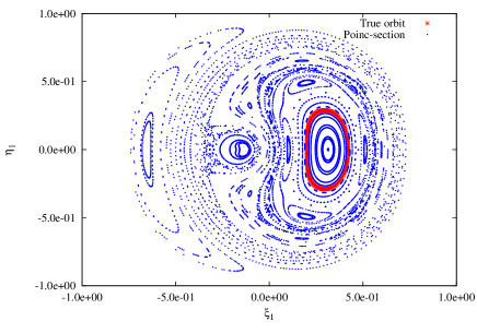
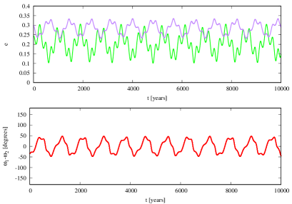
Figure 1: Study of the Hamiltonian dynamics defined by $H^{({\rm sec})}$ in formula (10). On the right, Poincaré sections: the orbit with initial conditions compatible with the observations is plotted in red, while the orbits referring to other initial conditions at the same energy level are in blue. In the top-right box, behavior of the planetary eccentricities as a function of time: the plots in green and in purple refer to $\upsilon$ And c and $\upsilon$ And d, resp. On bottom-right, evolution of the difference of the pericenters arguments. All the curves reported on the right refer just to the true orbit characterized by the initial values reported in Table 1.

In the first box of Figure 1, we report the Poincaré sections of the orbital motions induced by the Hamiltonian flow of $H^{({\rm sec})}$. They are plotted in correspondence of the hyperplane $\eta_{2}=0$, with $\xi_{2}>0$. They refer to both the initial values of the orbital elements reported in Table 1 (characterizing what we will call, hereafter, true secular orbit or, for short, true orbit) and several other initial conditions having the same energy. Looking at Figure 1, a few remarks are in order; they are going to play a fundamental role in the subsequent design of our approach. Firstly, for most of the Poincaré sections the chaotic effects are not easily remarkable and the two most regular zones are in the neighborhood of two fixed points (located on the axis of the abscissas, i.e., with $\eta_{1}=0$). Moreover, the true secular orbit describes a closed curve that is around one of these points and does not include the origin. This is in agreement with the fact that the difference of the arguments of the pericenters librates without completing a full rotation, as it can be seen in the plot on the bottom–right of Figure 1, where the dynamical evolution of the orbital elements is computed by applying, in reverse order, all the definitions introduced in the previous subsections 2.1–2.2. Finally, the plots of the eccentricities in the top–right box of Figure 1 highlight that their values oscillate in a range between $0.1$ and $0.35$. This makes clear that we have to develop an approach substantially different with respect to that described in [39], which has been designed to study planetary models similar to that including Sun, Jupiter and Saturn, where the eccentricities are always smaller than $0.1$ and the difference of the perihelion arguments is in a regime of full rotation.

3 Librational KAM tori for the secular model

In this section we describe the technique for the construction of KAM tori in the case of the secular Hamiltonian model defined in formula (13), with a specific focus on the one which corresponds to the true secular orbit, according to the definition introduced in the previous section.

In order to easily study the model, it is useful to define a set of action-angle variables $({\bm{J}},{\bm{\psi}})$ via the canonical transformation

$$\xi_{j}=\sqrt{2J_{j}}\cos\psi_{j}\ ,\qquad\eta_{j}=\sqrt{2J_{j}}\sin\psi_{j}\ ,\qquad\forall\ j=1,2,$$ (12)

being $({\bm{\xi}},{\bm{\eta}})$ the variables introduced in order to properly define the secular model. It is important to recall that the angles $(\psi_{1},\psi_{2})$ associated to these secular variables are nearly equal to the arguments of the pericenters $(\omega_{1},\omega_{2})$, apart from a small correction due to the (close-the-identity) transformation of coordinates induced by the application of the Lie series $\exp\mathcal{L}_{\chi_{1}^{(\mathcal{O}2)}}$ to the Hamiltonian of the three-body planetary problem. After this canonical change of coordinates, the Hamiltonian (11) reads

$$H^{({\rm I})}(\bm{J},\bm{\psi})=\sum_{\ell=1}^{N_{S}/2}h_{\ell}^{({\rm I})}(\bm{J},\bm{\psi})\ ,$$ (13)

where $h_{\ell}$ is an homogeneous polynomial function of degree $2\ell$ in the square roots of actions $\bm{J}$ and a trigonometric polynomial of degree $2\ell$ in angles $\bm{\psi}\,$, i.e., it writes

$$h_{\ell}^{({\rm I})}({\bm{J}},{\bm{\psi}})=\sum_{i_{1}+i_{2}=2\ell}\,\sum_{j_{1}=0}^{i_{1}}\sum_{j_{2}=0}^{i_{2}}c_{\ell;i_{1};i_{2};j_{1};j_{2}}^{({\rm I})}\sqrt{J_{1}^{i_{1}}J_{2}^{i_{2}}}\cos\big{[}(i_{1}-2j_{1})\psi_{1}+(i_{2}-2j_{2})\psi_{2}\big{]}\,.$$ (14)

The occurrence of only cosines in the formula above with particular Fourier harmonics in their arguments is again due to the relations induced by the D’Alembert rules.

It is now convenient to introduce a new set of variables $({\bm{I}},{\bm{\varphi}})$, where one of the angles is the difference between the pericenter arguments of the two planets, while the actions are defined so as to make the change of coordinates canonical; therefore, the transformation of coordinates is expressed as follows:

$$\varphi_{1}=\psi_{1}-\psi_{2}\ ,\quad\varphi_{2}=\psi_{2}\ ,\quad I_{1}=J_{1}\ ,\quad I_{2}=J_{2}+J_{1}\ .$$ (15)

Moreover, let us now introduce the canonical polynomial variables $({\bm{x}},{\bm{y}})$ defined as

$$x_{j}=\sqrt{2I_{j}}\cos\varphi_{j}\ ,\qquad y_{j}=\sqrt{2I_{j}}\sin\varphi_{j}\ ,\qquad\forall\ j=1,2\ .$$ (16)

Let us now remark that making Poincaré sections with respect to the hyperplane $\eta_{2}=0$, when $\xi_{2}>0$ is equivalent to impose $\psi_{2}=0$, because of the definitions in (12). Therefore, looking at formulæ (15)–(16), one can easily realize that the drawing on the left of Figure 1 can be seen as a plot of the Poincaré sections in coordinates $(x_{1}\,,\,y_{1})$ with respect to $y_{2}=0$ and with the additional condition $x_{2}>0$. Revisiting the plot of the true secular orbit in the bottom–right box of Figure 1 and in the context of the new canonical variables is extremely interesting, because it makes clear that $\varphi_{1}$ is librating around the origin. In fact, we have that $\varphi_{1}=\psi_{1}-\psi_{2}\simeq\omega_{1}-\omega_{2}\,$, because the relation between these differences of angles is given by the transformation induced by the application of the Lie series $\exp\mathcal{L}_{\chi_{1}^{(\mathcal{O}2)}}$, that is close to the identity. By comparison with the behavior of the difference between the pericenter arguments in Figure 1, it is natural to expect that also the angle $\varphi_{1}$ is librating in a range that cannot be much larger than $[-50^{\circ},50^{\circ}]$.

Focusing on the axis of the abscissas of the Poincaré sections plotted in blue in Figure 1, one can remark that there is a fixed point located at $(\xi_{1}\simeq 0.3\,,\,\eta_{1}=0)$; moreover, it is surrounded by orbits lying on nearly elliptical closed curves. It can be seen as a periodic orbit, namely a lower dimensional (here, one-dimensional) torus that in this case is transversely elliptic. From an astronomical point of view, it is characterized by the fact that the pericenters stay nearly perfectly anti-aligned, being $0=\varphi_{1}\simeq\omega_{1}-\omega_{2}\,$. The true secular orbit is in libration around such an extremely peculiar configuration. The Poincaré sections in Figure 1 are structured in such a way that it is natural to expect that the periodic solution corresponding to the anti-alignment of the pericenters is extremely robust. This property should allow the one-dimensional elliptic torus to influence the dynamics and the stability in its neighborhood and, in particular, for what concerns the true secular orbit. Therefore, we will proceed by first constructing that specific periodic solution which describes a full rotation of the angle $\varphi_{2}\,$, without any oscillation in the transverse directions corresponding to the pair of canonical variables $(I_{1}\,,\,\varphi_{1})$ or, equivalently, $(x_{1}\,,\,y_{1})$.

3.1 Construction of the lower dimensional elliptic torus

The construction of the wanted periodic orbit can be done with a normal form algorithm similar to the one described in [35] and [7], after having defined suitable transformations of coordinates in order to be approximately centered around the solution we aim to build. The location of the wanted periodic orbit can be determined numerically with a method that is based on the frequency analysis (see, e.g., [21]), in short FA, hereafter. In the following, we briefly recall the main features of such a computational procedure, that is accurately described, e.g., in [7].

We look for a set of initial conditions close to an orbit in which the angle $\varphi_{2}$ rotates periodically, without oscillations in the transverse plan $(x_{1},y_{1})$. The true orbit is near that solution as there is a small libration of the angle $\varphi_{1}$. Therefore, we start by extracting from the numerical signal $x_{2}(t)+{\bf i}y_{2}(t)$, which is related to the motion of the angle $\varphi_{2}$ of the true orbit, its main frequency $\nu_{2,1}\,$, being $\sum_{s=1}^{\mathcal{N}_{C}}A_{2,s}e^{{\bf i}(\nu_{2,s}t+\varphi_{2,s})}$ the decomposition obtained by using FA, where $\mathcal{N}_{C}$ is the number of components considered and, hereafter, we assume that the amplitudes $A_{j,s}>0$ are in descending order with respect to $s=1,\ldots,\mathcal{N}_{C}\ \forall\ j=1,2$. Then, we focus on the signal of the other pair of canonical coordinates, i.e., $x_{1}(t)+{\bf i}y_{1}(t)\simeq\sum_{s=1}^{\mathcal{N}_{C}}A_{1,s}e^{{\bf i}(\nu_{1,s}t+\varphi_{1,s})}$, that is related to the librational motion of the angle $\varphi_{1}$; therefore, we expect to find contributions given by frequencies that are not integer multiples of $\nu_{2,1}\,$. We define as a new initial condition $\tilde{x}_{j}(0)+{\bf i}\tilde{y}_{j}(0)=\sum_{s=1}^{\mathcal{N}_{C}}\tilde{A}_{j,s}e^{{\bf i}\varphi_{j,s}}$, where we are considering only the components $\tilde{A}_{j,s}$ related to the frequencies $\nu_{j,s}$ that are integer multiples of $\nu_{2,1}$, otherwise we put the corresponding amplitude $A_{j,s}=0$. We integrate the equation of motion with this other initial condition and we iterate the procedure until both the signals can be decomposed, up to a tolerance threshold, in terms of a single frequency $\nu_{2,1}$.

Once that we have found the initial condition $({\bm{x}}^{\star},{\bm{y}}^{\star})$ for a periodic solution, we are able to introduce a first translation on the action $I_{2}$ by defining $p=I_{2}-I^{\star}$, where $I^{\star}=(x_{2}^{\star 2}+y_{2}^{\star 2})/2$, and to expand the Hamiltonian in Taylor series around $p=0$. Then, we divide the variables in two different couples: we rename the angle $\varphi_{2}$ as $q$, so that $(p,q)\in\mathbb{R}\times\mathbb{T}$ is the action-angle couple describing the periodic motion, while we still use the polynomial variables $(x_{1},y_{1})$ for the motion transverse to the periodic orbit. The last preliminary translation is on $x_{1}\,$, in order to have expansions around the value $x_{1}^{\star}$, given by the initial condition computed numerically. Let us emphasize that, since the fixed point we are trying to approximate in Figure 1 corresponds to $\varphi_{1}=0$, we have that $y_{1}=0$ and here a translation is not needed. Finally, before starting with the construction of a better approximation of the elliptic torus by putting the Hamiltonian in a suitable normal form, we rescale the transverse variables $(\bar{x}_{1},y_{1})$, being $\bar{x}_{1}=x_{1}-x_{1}^{\star}$, in such a way that the quadratic part in the new variables $(x,y)$ is in the form $\Omega^{\star}(x^{2}+y^{2})/2$. This rescaling can be done by a canonical transformation as the quadratic part does not have any mixed term $\bar{x}_{1}y_{1}$ and the coefficients of $\bar{x}_{1}^{2}$ and $y_{1}^{2}$ have the same sign, because of the proximity to an elliptic equilibrium point. Thus, since such a quadratic part is in the preliminary form $a\bar{x}_{1}^{2}+by_{1}^{2}$, it suffices to define the new variables $(x,y)$ as $x=\sqrt[4]{\frac{a}{b}}\,\bar{x}_{1},\ y=\sqrt[4]{\frac{b}{a}}\,y_{1}$.

After all these transformations, the expansion of the Hamiltonian can be written as follows:

$$H(p,q,x,y)= E+\omega^{\star}\ p+\Omega^{\star}\frac{x^{2}+y^{2}}{2}+\mathcal{F}_{\rm{h.o.t.}}(p,q,x,y)+$$ (17)

$$+\sum_{s>0}f_{0}^{(s)}(q)+\sum_{s>0}f_{1}^{(s)}(q,x,y)+\sum_{s>0}f_{2}^{(s)}(p,q,x,y)\,,$$

where each $f_{\ell}^{(s)}$ is a function in the variables $(p,q,x,y)$, whose corresponding Taylor-Fourier series is given by a finite number of terms. More precisely, $\ell$ is its total degree in the square root of the actions, i.e., $\ell=2j_{1}+j_{2}$, where $j_{1}$ is the degree in $p$ and $j_{2}$ the degree in $(x,y)$, while $2s$ is the maximum trigonometrical degree in the angle $q$. In (17), we have highlighted the terms with total degree in the square root of the actions up to $2$ and we have collected all the terms of higher order in $\mathcal{F}_{\rm{h.o.t.}}$. This choice is coherent with our purpose to start the iteration of an algorithm for the construction of a lower dimensional elliptic torus, by following the approach described in [35] and in [7]; this is feasible provided that the terms appearing in the second row of (17) are small enough with respect to those in the first row. Furthermore, $E$ is a constant term, meaning just the energy level of the invariant manifold $p=x=y=0$ in the limit case with $f_{0}^{(s)}=f_{1}^{(s)}=f_{2}^{(s)}=0\ \forall\ s>0$. In the following, we will just recall the procedure, by emphasizing what is necessary to adapt in such a way to fit with the present context.

The expansion of the Hamiltonian in (17) can be visually rearranged as

$$\>{\vdots}$$

(18)

where $\omega^{(0)}=\omega^{*}$, $\Omega^{(0)}=\Omega^{*}$ and $E^{(0)}=E$, the first upper index of the polynomial terms and of the Hamiltonian refers to the normalization step, while the second one refers to the trigonometrical degree in $q$. In the normalization procedure, we will define a sequence of canonical transformations, with the aim of removing the contributions appearing in the first three rows, that are terms having total degree in the square root of the actions up to $2$, except for the part in normal form that does not depend on the angle $q$. In order to avoid the proliferation of symbols, by abuse of notation we are going to use the same name for the variables, even if we are indeed applying several changes of coordinates.

The first change of coordinates is identified by the generating function $\chi_{1}^{(1)}(q)$, of trigonometrical degree up to $2$ in the angle $q$, which solves the following homological equation:

$$\left\{\chi_{0}^{(1)},\ \omega^{(0)}p\right\}+f_{0}^{(0,1)}(q)=\langle f_{0}^{(0,1)}(q)\rangle_{q}.$$ (19)

Let us stress that the term in the r.h.s. of the equation above is constant because it denotes the angular average of $f_{0}^{(0,1)}$; therefore, it can change the energy value but it has not any role in the Hamilton equations.

We will obtain an Hamiltonian $H^{(I;1)}=\exp\mathcal{L}_{\chi_{0}^{(1)}}H^{(0)}$ with $f_{0}^{(I;1,1)}(q)=0$, where the new upper index $I$ is now referred to the first substep and $E^{(1)}=E^{(0)}+\langle f_{0}^{(0,1)}(q)\rangle_{q}$. In order to better understand the following, it is convenient to imagine the expansion of $H^{(I;1)}$ as in formula (18), by replacing each term $f_{\ell}^{(0,s)}$ with $f_{\ell}^{(I;1,s)}$, having the same functional properties, i.e., $\ell$ is the total degree in the square root of the actions, while $2s$ is the maximum trigonometrical degree in the angle $q$.

The second substep is meant to eliminate terms linear in the square root of the actions. We introduce $\chi_{1}^{(1)}(q,x,y)$, linear in $(x,y)$ and of trigonometrical degree up to $2$ in the angle $q$, such that

$$\left\{\chi_{1}^{(1)},\ \omega^{(0)}p+\Omega^{(0)}\frac{x^{2}+y^{2}}{2}\right\}+f_{1}^{(I;1,1)}(q,x,y)=0.$$ (20)

In this case, since the origin of the transverse variables corresponds to an elliptic equilibrium point, terms that are linear in $x$ and $y$ with non-zero angular average cannot appear in the r.h.s. of the equation above. Therefore, we are able to define $H^{(II;1)}=\exp\mathcal{L}_{\chi_{1}^{(1)}}H^{(I;1)}$ with $f_{1}^{(II;1,1)}(q,x,y)=0$. In order to better understand the following, once again, it is convenient to imagine the expansion of $H^{(II;1)}$ as in formula (18), by replacing each term $f_{\ell}^{(0,s)}$ with the corresponding one, that is denoted with $f_{\ell}^{(II;1,s)}$ and has the same functional properties.

The third substep aims to remove terms linear in the actions that depend on the angle $q$ and it is split in two different stages, each of them responsible for the removal of terms linear in $p$ or quadratic in $(x,y)$. We define $X_{2}^{(1)}(p,q)$, linear in $p$ and of trigonometrical degree $2$ in the angle $q$, such that

$$\left\{X_{2}^{(1)},\ \omega^{(0)}p\right\}+f_{2}^{(II;1,1)}(p,q)=\langle f_{2}^{(II;1,1)}(p,q)\rangle_{q};$$ (21)

we define $Y_{2}^{(1)}(q,x,y)$, quadratic in $(x,y)$ and of trigonometrical degree up to $2$ in the angles $q$, such that

$$\left\{Y_{2}^{(1)},\ \omega^{(0)}p+\Omega^{(0)}\frac{x^{2}+y^{2}}{2}\right\}+f_{2}^{(II;1,1)}(q,x,y)=\langle f_{2}^{(II;1,1)}(q,x,y)\rangle_{q}.$$ (22)

In both the previous formulæ we have denoted the kind of terms by writing explicitly the dependence on the variables. The terms that we cannot remove with these transformations have non-zero average on $q$; moreover, they are linear in the actions and essentially of the same type of the normal form. Therefore, they are added to the normal form part itself by defining new frequencies $\omega^{(1)}$ and $\Omega^{(1)}$ as follows:

$$\omega^{(1)}p =\omega^{(0)}p+\langle f_{2}^{({\rm II};1,1)}(p,q)\rangle_{q}\,,$$ (23)

$$\Omega^{(1)}\frac{x^{2}+y^{2}}{2} =\Omega^{(0)}\frac{x^{2}+y^{2}}{2}+\langle f_{2}^{({\rm II};1,1)}(q,x,y)\rangle_{q}\,,$$ (24)

where in the last formula, $\langle f_{2}^{({\rm II};1,1)}(q,x,y)\rangle_{q}$ is put in diagonal form. This can be done perturbatively by using the Lie transform, i.e., by performing an infinite sequence of Lie series (see [15] and [7] for further details). Therefore, the first normalization step is completed by applying $\exp\mathcal{L}_{X_{2}^{(1)}}$, $\exp\mathcal{L}_{Y_{2}^{(1)}}$ and the Lie transform (that has been mentioned just above) to the intermediate Hamiltonian $H^{(II;1)}$. This allows us to fully determine $H^{(1)}$, whose expansion can be represented as in formula (18), by replacing each term $f_{\ell}^{(0,s)}$ with the corresponding one, i.e., $f_{\ell}^{(1,s)}$, having the same functional properties. Of course, for what concerns the new Hamiltonian $H^{(1)}$, in the expansion analogous to that written in (18), the angular velocities $\omega^{(1)}$, $\Omega^{(1)}$ and the the energy level $E^{(1)}$ will appear in place of $\omega^{(0)}$, $\Omega^{(0)}$ and $E^{(0)}$, respectively; moreover, in the first three cells of the second row, $f_{\ell}^{(0,1)}$ shall be replaced by $f_{\ell}^{(1,1)}=0$ for $\ell=0,\,1,\,2$, accordingly with the definitions of the homological equations (19)–(22).

The generic $r$-th step is performed in the same way, with the only difference that the generating functions $\chi_{0}^{(r)}$, $\chi_{1}^{(r)}$, $X_{2}^{(r)}$ and $Y_{2}^{(r)}$ are determined in such a way to remove the perturbing terms of trigonometrical degree up to $2r$. Let us stress the fact that, in order to solve the homological equations and to let the whole procedure to be convergent, some non-resonance conditions have to be satisfied. These requirements can be summarized by the following formula:

$$\min_{{0\leq|k|\leq 2r,\ 0\leq|\ell|\leq 2}\atop{|k|+|\ell|>0}}\Big{|}k\omega^{(r-1)}+\ell\Omega^{(r-1)}\Big{|}\geq\frac{\gamma}{|k|^{\tau}+1}\ \ {\rm with}\ \gamma>0,\ \tau>0\ ,$$ (25)

where let us emphasize that here, for $\ell=0$, we do not have small divisors, since we deal with a single frequency (that is related to the wanted periodic orbit) instead of a vector.

The convenience of such a procedure is highlighted by the fact that, after an infinite number of iterations of the algorithm, the Hamiltonian reads

$$H^{(\infty)}=E^{(\infty)}+\omega^{(\infty)}\ p+\Omega^{(\infty)}\,\frac{x^{2}+y^{2}}{2}+\sum_{s\geq 0}\sum_{\ell>2}f_{\ell}^{(\infty,s)}(p,q,x,y)$$ (26)

and, therefore, it is evident that $(0,q_{0}+\omega^{(\infty)}t,0,0)$ is a periodic orbit. Besides, from a practical point of view, we iterate the algorithm only for a finite number of steps and we construct an approximation of the periodic orbit, being the final Hamiltonian after $\bar{r}$ steps

$$H^{(\bar{r})}=E^{(\bar{r})}+\omega^{(\bar{r})}\ p+\Omega^{(\bar{r})}\,\frac{x^{2}+y^{2}}{2}+\sum_{s\geq 0}\sum_{\ell>2}f_{\ell}^{(\bar{r},s)}(p,q,x,y)+\sum_{s>\bar{r}}\sum_{\ell\geq 0}^{2}f_{\ell}^{(\bar{r},s)}(p,q,x,y)\ ,$$ (27)

where $\sum_{s>\bar{r}}\sum_{\ell\geq 0}^{2}f_{\ell}^{(\bar{r},s)}(p,q,x,y)$ is the remainder of the normal form.

Let us conclude this subsection with a comment about the choice of the initial translations $I^{\star}$ and $x_{1}^{\star}$. Indeed, if they are accurate enough, we expect that the algorithm will converge to an approximated periodic orbit defined by $(\omega^{(\bar{r})},\ \Omega^{(\bar{r})})$ close to the one we are aiming at, namely the one we have found by using the FA. However, at this level, the value of $I^{\star}$ can be improved, in order to “automatically” lead to a periodic orbit as close as possible to the numerical one. This is done by using a Newton method to solve the equation $E(I)=\bar{E}$, where $E(I)$ is the energy associated to the (approximated) periodic orbit we have found by using the translation $I$ and iterating the algorithm for a finite number of steps, while $\bar{E}$ is the energy of the periodic orbit found by using the FA. The same Newton method can be used to improve the translation $x_{1}^{\star}$ and, therefore, to remove from the Hamiltonian the terms linear in $(\bar{x}_{1},y_{1})$: the equation to be solved in this case is $\frac{\partial\langle H\rangle_{q}}{\partial{x}}(0,0,0,0)=0$, where we recall that $x=\sqrt[4]{\frac{a}{b}}\,\bar{x}_{1}$. The initial translations $I^{\star}$ and $x_{1}^{\star}$ as defined at the beginning of this subsection are in general good enough initial guesses for ensuring the simultaneous convergence of both the Newton methods.

3.2 Construction of the librational KAM torus

The normal form related to the elliptic torus is now considered as the starting point for the construction of the full dimensional KAM tori around it and, in particular, the invariant surface corresponding to initial conditions compatible with the observations. Since we cannot derive the secular frequencies by the observations, we use again the FA to compute the frequency vector $\tilde{{\bm{\omega}}}$, being $\tilde{\omega}_{1}$ and $\tilde{\omega}_{2}$ the frequencies associated to the rotation of the angle $\varphi_{2}$ and to the oscillations of the angle $\varphi_{1}$.

Initially, we translate again the coordinates, in order to be centered around a good approximation of the true orbit. The variables $(x,y)$ for which the Hamiltonian is in normal form for elliptic tori are centered around the equilibrium point, but we can identify the right translation on the action $I=(x^{2}+y^{2})/2$ by expressing the initial conditions of the true orbit in these coordinates; then, we can expand the Hamiltonian in Taylor series around $p_{2}=0$, being $p_{2}=I-I_{2}^{\star}$, where $I_{2}^{\star}$ is the value of the action at time $0$ of the true orbit. Moreover, we rename the angle associated to the transverse polynomial variables $(x,y)$ as $q_{2}$ and we recollect the variables with the other action-angle couple $(p,q)$ (renamed as $(p_{1},q_{1})$), so that the Hamiltonian is now expressed in the variables $({\bm{p}},{\bm{q}})$, being the first couple referred to the periodic motion of the angle $\varphi_{2}$, while the second one is referred to the libration as it is measured from the elliptic torus.

We are ready to proceed with a classic algorithm for the construction of the Kolmogorov normal form, by following the approach described in section 4 of [13]. First, the expansion of the initial Hamiltonian $\mathcal{H}^{(0)}$ (that has been obtained from $H^{(\bar{r})}$ written in (27), by applying the translation described just above) can be visually reorganized as follows:

$$\>{\vdots}$$

(28)

being the generic term $f_{j}^{(0,s)}$ an homogeneous polynomial of degree $j$ in the actions $\bm{p}$ and of trigonometrical degree up to $2s$ in $\bm{q}$. The Kolmogorov’s normalization algorithm requires to remove all the terms of the Hamiltonian (28) of degree $0$ or $1$ in the actions $\bm{p}$, with the exception of the term ${\bm{\omega}^{(0)}}\cdot\bm{p}\,$. Let us stress that an accurate definition of the translation vector $I_{2}^{\star}$ should lead to a frequency vector ${\bm{\omega}}^{(0)}\simeq\tilde{{\bm{\omega}}}$.

In order to construct the normal form, we start by determining the generating function $X^{(1)}({\bm{q}})$ such that

$$\{X^{(1)},\bm{\omega}^{(0)}\cdot\bm{p}\}+f_{0}^{(0,1)}=\langle f_{0}^{(0,1)}\rangle_{{\bm{q}}}\ ,$$ (29)

where $X^{(1)}$ is a trigonometric polynomial of degree $2$. The term $\langle f_{0}^{(0,1)}\rangle_{{\bm{q}}}$ will contribute to the energy as a new constant term, to be summed up to the initial value of the energy $E^{(0)}$ (again, close to the energy of the true orbit). We will then obtain a new Hamiltonian $\hat{\mathcal{H}}^{(1)}=\exp\mathcal{L}_{X^{(1)}}\mathcal{H}^{(0)}$, whose expansion can be visualized as in (28) with generic terms now denoted by $\hat{f}_{j}^{(1,s)}$, being $\hat{f}_{0}^{(1,1)}=0$ as a consequence of equation (29).

We proceed in an analogous way to complete this first Kolmogorov’s normalization step: we compute the generating function $\chi_{2}^{(1)}(\bm{p},\bm{q})$ such that

$$\{\chi_{2}^{(1)},\bm{\omega}^{(0)}\cdot\bm{p}\}+\hat{f}_{1}^{(1,1)}=\langle\hat{f}_{1}^{(1,1)}\rangle_{\bm{q}}\ ;$$ (30)

therefore, $\chi_{2}^{(1)}$ will be linear in $\bm{p}$ and of trigonometrical degree equal to 2 in $\bm{q}$. Let us remark that it is possible to solve the previous homological equations (29) and (30), provided that $|{\bm{k}}\cdot{\bm{\omega}}^{(0)}|>0$ for ${\bm{k}}\in\mathbb{Z}^{2}$ with $|{\bm{k}}|=1,2$ , being $|{\bm{k}}|=|k_{1}|+|k_{2}|$ .

If we do not introduce a further change of coordinates with the aim of fixing the frequency vector of the torus in construction, we will need to define a new frequency vector $\bm{{\bm{\omega}}}^{(1)}$ in such a way that

$$\bm{\omega}^{(1)}\cdot\bm{p}=\bm{\omega}^{(0)}\cdot\bm{p}+\langle\hat{f}_{1}^{(1,1)}\rangle_{\bm{q}}\ .$$ (31)

Therefore, we will obtain the new Hamiltonian $\mathcal{H}^{(1)}=\exp\mathcal{L}_{\chi_{2}^{(1)}}\hat{\mathcal{H}}^{(1)}$, whose expansion can be again visualized as in (28), where each generic term $f_{j}^{(0,s)}$ is replaced with the corresponding one, i.e., $f_{j}^{(1,s)}$, having the same functional properties; moreover, $f_{0}^{(1,1)}$ and $f_{1}^{(1,1)}$ are now equal to 0.

The generic $r$-th normalization step can be performed in the same way, because the Hamiltonian expansion $\mathcal{H}^{(r-1)}$, if we replace the upper index $0$ with $r-1$, is of the same form as that described in (28). Although the procedure is rather standard, we retain useful to report here some additional detail about the construction, being also necessary for the following discussions about the convergence of the procedure. The generating functions $X^{(r)}$ and $\chi_{2}^{(r)}$ are introduced by solving the homological equations obtained by replacing the upper indices $0$ and $1$ with $r-1$ and $r$, respectively, in formulæ (29) and (30) and they can be written as follows:

$$X^{(r)}({\bm{q}})=\sum_{0<|{\bm{k}}|\leq 2r}-c_{{\bm{k}}}^{(r-1,r)}\frac{e^{i{\bm{k}}\cdot{\bm{q}}}}{i{\bm{k}}\cdot{\bm{\omega}}^{(r-1)}}\ ,$$ (32)

being $f_{0}^{(r-1,r)}({\bm{q}})=\sum_{0<|{\bm{k}}|\leq 2r}c_{{\bm{k}}}^{(r-1,r)}e^{i{\bm{k}}\cdot{\bm{q}}}$ the term that does not depend on the actions ${\bm{p}}$ to be removed at the $r$-th step, while the second generating function is defined as

$$\chi_{2}^{(r)}({\bm{p}},{\bm{q}})=\sum_{j=1}^{2}\sum_{0<|{\bm{k}}|\leq 2r}-c_{j,{\bm{k}}}^{(r-1,r)}p_{j}\ \frac{e^{i{\bm{k}}\cdot{\bm{q}}}}{i{\bm{k}}\cdot{\bm{\omega}}^{(r-1)}}\ ,$$ (33)

being $\hat{f}_{1}^{(r-1,r)}({\bm{p}},{\bm{q}})=\sum_{j=1}^{2}\sum_{0<|{\bm{k}}|\leq 2r}c_{j,{\bm{k}}}^{(r-1,r)}p_{j}\ e^{i{\bm{k}}\cdot{\bm{q}}}$ the expansion of the unwanted term that is met at the $r$-th step and is linear in the actions ${\bm{p}}$. Therefore, the homological equations can be solved provided that the following non-resonance condition holds true:

$$|{\bm{k}}\cdot{\bm{\omega}}^{(r-1)}|>0\ ,\qquad\forall\ {\bm{k}}\in\mathbb{Z}^{2}\setminus\{{\bm{0}}\}\ {\rm with}\ |{\bm{k}}|\leq 2r\ .$$ (34)

The new Hamiltonian is finally given by

$$\mathcal{H}^{(r)}=\exp\mathcal{L}_{\chi_{2}^{(r)}}\hat{\mathcal{H}}^{(r)}\quad{\rm with}\quad\hat{\mathcal{H}}^{(r)}=\exp\mathcal{L}_{X^{(r)}}\mathcal{H}^{(r-1)}\ ,$$ (35)

where the effect on the expansions that is due to the application of the Lie series can be fully described in the following way. In the spirit of a programming language, we define the intermediate functions $\hat{f}_{\ell}^{(r,s)}=f_{\ell}^{(r-1,s)}\ \forall\ \ell,s\geq 0$ and then the contributions due to the Lie derivatives with respect to the generating function $X^{(r)}$, that is an operator decreasing by $1$ the degree in the actions and increasing by $2r$ the trigonometrical degree in the angles, are added in such a way that

$$\hat{f}_{\ell-j}^{(r,jr+s)}\hookleftarrow\frac{1}{j!}\mathcal{L}_{X^{(r)}}^{j}f_{\ell}^{(r-1,s)}\,,\quad{\rm for}\ 1\leq j\leq\ell,\ s\geq 0\ ,$$ (36)

where with the notation $a\hookleftarrow b$ we mean that the quantity $a$ is redefined so as to be equal $a+b$. For what concerns the Lie derivative with respect to the generating function $\chi_{2}^{(r)}$, it does not change the degree in the actions while it increases by $2r$ the trigonometrical degree in the angles, therefore, we can define $f_{\ell}^{(r,s)}=\hat{f}_{\ell}^{(r,s)}$ $\forall\ \ell,s\geq 0$ and then add all the other generated terms as follows:

$$f_{\ell}^{(r,jr+s)}\hookleftarrow\frac{1}{j!}\mathcal{L}_{\chi_{2}^{(r)}}^{j}\hat{f}_{\ell}^{(r-1,s)}\,,\quad{\rm for}\ j\geq 1,\ \ell\geq 0,\ s\geq 0\ .$$ (37)

The algorithm is iterated up to a finite number of steps $\bar{r}$, thus at the end we have an approximated torus with frequency vector ${\bm{\omega}}^{(\bar{r})}$, being the $r$-th Hamiltonian in the form

$$\mathcal{H}^{(\bar{r})}=E^{(\bar{r})}+{\bm{\omega}}^{(\bar{r})}\cdot{\bm{p}}+\sum_{s\geq 0}\sum_{\ell\geq 2}f_{\ell}^{(\bar{r},s)}({\bm{p}},{\bm{q}})+\sum_{s>\bar{r}}\sum_{\ell=0}^{1}f_{\ell}^{(\bar{r},s)}({\bm{p}},{\bm{q}})\ .$$ (38)

Once again, we recall that if the initial translation $I_{2}^{\star}$ is accurate enough, we should end up with a torus close to the real one, with ${\bm{\omega}}^{(\bar{r})}\simeq\tilde{{\bm{\omega}}}$. Also in this case, the shift on the action value $I_{2}^{\star}$ can be improved by means of a Newton method; furthermore, it could be useful to add an appropriate extra translation to the action $p_{1}$, that, we recall, is already expanded around $I^{\star}$, i.e., the initial value of the action of the periodic orbit. The aim is to find the translations $\tilde{I}_{1}$ and $\tilde{I}_{2}$ such that ${\bm{\omega}}^{(\bar{r})}(\tilde{I}_{1},\tilde{I}_{2})=\tilde{{\bm{\omega}}}$, being the translation applied before the iteration of the Kolmogorov’s algorithm defined as

$$\chi({\bm{q}})=\tilde{{\bm{I}}}\cdot{\bm{q}}\,.$$ (39)

The initial translations are iteratively adjusted by applying the following refinement formula:

$$\tilde{{\bm{I}}}^{(n)}=\tilde{{\bm{I}}}^{(n-1)}-\frac{\Delta{\bm{\omega}}(\tilde{{\bm{I}}}^{(n-1)})}{\mathcal{J}(\tilde{{\bm{I}}}^{(n-1)})}$$ (40)

where $\Delta{\bm{\omega}}(\tilde{{\bm{I}}})={\bm{\omega}}^{(\bar{r})}(\tilde{{\bm{I}}})-\tilde{{\bm{\omega}}}$, $\tilde{{\bm{I}}}^{(0)}=(0,I_{2}^{\star})$ and the Jacobian $\mathcal{J}(\tilde{{\bm{I}}})$ of the function ${\bm{\omega}}(\tilde{{\bm{I}}})$ is numerically computed, being the evaluation of such a function rather implicit.

After having found $\tilde{I}_{1}$ and $\tilde{I}_{2}$ such that the approximation of the torus is good enough, we iterate one last time the algorithm constructing the Kolmogorov normal form $\mathcal{K}^{(\infty)}$ (written in (43)), in this case by keeping fixed the value of the angular velocity vector so as to be equal to $\tilde{{\bm{\omega}}}$ by means of a translation to be performed at each normalization step. The algorithm is restarted from the new initial Hamiltonian $\mathcal{K}^{(0)}$ that is defined as

$$\mathcal{K}^{(0)}=E^{(0)}+\tilde{{\bm{\omega}}}\cdot{\bm{p}}+\sum_{s\geq 0}\sum_{\ell\geq 2}f_{\ell}^{(0,s)}({\bm{p}},{\bm{q}})+\sum_{s\geq 1}\sum_{\ell=0}^{1}f_{\ell}^{(0,s)}({\bm{p}},{\bm{q}}),$$ (41)

where the terms appearing in such a formula are obtained by the corresponding ones in the expansion of $\mathcal{H}^{(\bar{r})}$ in (38), after having translated the actions by a vector ${\bm{\xi}}^{(0)}$ such that ${\bm{\omega}}^{(\bar{r})}+C^{(0)}{\bm{\xi}}^{(0)}=\tilde{{\bm{\omega}}}$, where $C^{(0)}={\rm Hess}\sum_{s=0}^{\bar{r}}\langle f_{2}^{(\bar{r},s)}\rangle_{{\bm{q}}}$. Once again, we do not change the symbols $E$ and $f$ after having performed a translation (that is a canonical transformation) by abuse of notation. Therefore, the main difference with the algorithm previously described is that we have to compute another generating function ${\bm{\xi}}^{(r)}\cdot{\bm{q}}$ at each step $r$, so as to solve the following homological equation

$$\left\{{\bm{\xi}}^{(r)}\cdot{\bm{q}},\frac{1}{2}C^{(r)}{\bm{p}}\cdot{\bm{p}}\right\}+{\bm{\omega}}^{(r)}\cdot{\bm{p}}=\tilde{{\bm{\omega}}}\cdot{\bm{p}},$$ (42)

where $\frac{1}{2}C^{(r)}{\bm{p}}\cdot{\bm{p}}$ is the part in normal form that is quadratic in ${\bm{p}}$, i.e., $\sum_{s=0}^{r-1}\langle f_{2}^{(r-1,s)}\rangle_{{\bm{q}}}$. Moreover, the $r$-th normalization step is given by $\hat{\mathcal{K}}^{(r)}=\exp\mathcal{L}_{\chi_{1}^{(r)}}\mathcal{K}^{(r-1)}$ and $\mathcal{K}^{(r)}=\exp\mathcal{L}_{\chi_{2}^{(r)}}\hat{\mathcal{K}}^{(r)}$, where the first generating function is taking into account also the translation, i.e., $\chi_{1}^{(r)}=X^{(r)}+{\bm{\xi}}^{(r)}\cdot{{\bm{q}}}$, while the solution for $X^{(r)}$ and $\chi_{2}^{(r)}$ is still given by equations (32)–(33), where ${\bm{\omega}}^{(r-1)}$ is replaced by $\tilde{{\bm{\omega}}}$.

Let us suppose to be able to iterate it ad infinitum the algorithm, then we would end up with an Hamiltonian of the form

$$\mathcal{K}^{(\infty)}(\bm{p},\bm{q})\,=\,\tilde{\bm{\omega}}\cdot\bm{p}+\mathcal{O}(\|{\bm{p}}\|^{2})\$$ (43)

and, by writing the corresponding equations of motion, it is easy to realize that the torus $\{{\bm{p}}={\bm{0}}\,,\ {\bm{q}}\in\mathbb{T}^{2}\}$ would be obviously invariant and the motion on it would be quasi-periodic and characterized by an angular velocity vector equal to $\tilde{{\bm{\omega}}}$. As in the case of the algorithm for the normal form for elliptic tori, we can explicitly iterate the algorithm only up to a finite normalization step and we can investigate the convergence of the procedure by controlling the decrease of the norm of the generating functions. Let us emphasize that, when the initial approximation is not good enough, the translations ${\bm{\xi}}^{(r)}\cdot{\bm{q}}$ introduced to keep the frequency fixed are not close to the identity and, therefore, the convergence of the procedure is prevented. This is the reason why we iterate the algorithm with fixed frequencies only at the end of the whole application of the Newton method, when we have approached better the aimed solution.

3.3 Computer-assisted proof of existence of KAM tori

We have found interesting to enqueue to the construction of the normal form a scheme of estimates in order to produce a computer-assisted proof of the existence of the specific invariant torus we are aiming at. For what concerns the KAM theorem, let us recall that there are different computer–assisted proofs in literature (see, e.g., [8] and [26]), that have been introduced introduced with the purpose of filling the gap between analytical theory and applications to Celestial Mechanics. Here, we follow the approach very recently described in [38] and in subsection 4.2 we will also show the results produced by using the codes included into the supplementary material related to that work. However, instead of simply claiming that there is a software package which can be used as a black-box in order to produce a computer–assisted proof of existence of KAM tori, we think that it is more convenient to briefly recall that approach and discuss its underlying ideas. This is made in our framework also with the purpose of clarifying how to implement such a computer–assisted proof with very concrete chances of success in other contexts.

In order to apply an appropriate version of the KAM theorem, let us define the Hamiltonian for which we want to prove the existence of the invariant torus by iterating one last time the Kolmogorov normalization algorithm with a proper scheme of estimates. Our generic $r-1$-th Hamiltonian now writes

$$\mathcal{K}^{(r-1)}=E^{(r-1)}+\tilde{{\bm{\omega}}}\cdot{\bm{p}}+\sum_{s\geq 0}\sum_{\ell\geq 2}f_{\ell}^{(r-1,s)}({\bm{p}},{\bm{q}})+\sum_{s\geq r}\sum_{\ell=0}^{1}f_{\ell}^{(r-1,s)}({\bm{p}},{\bm{q}})\ ,$$ (44)

since here we aim to iterate the algorithm for constructing the Kolmogorov normal form in the version keeping fixed the angular velocity vector $\tilde{{\bm{\omega}}}$. The remainder $\mathcal{R}^{(r-1)}=\sum_{s\geq r}\sum_{\ell=0}^{1}f_{\ell}^{(r-1,s)}({\bm{p}},{\bm{q}})$ is the quantity we are interested in estimating and reducing below the threshold value of applicability. Following the approach used in [6] and [38] which goes back to the technique developed in [9], we distinguish between terms for which we will explicitly compute the Kolmogorov normal form (with the help of an algebraic manipulator, see [17] for an introduction) up to $R_{\rm I}$-th step, terms for which we estimate the $\ell_{1}$-norms with constants $\mathcal{F}_{\ell}^{(r,s)}$ such that $\|f_{\ell}^{(r,s)}\|\leq\mathcal{F}_{\ell}^{(r,s)}$ (up to a maximal degree in the angles ${\bm{q}}$ that is equal to $2R_{\rm II}$) and the tail of infinite terms. In the case of the latter ones, we provide just an uniform estimate

$$\|f_{\ell}^{(r-1,s)}\|\leq a_{r-1}^{s}\,\zeta_{r-1}^{\ell}\,\mathcal{E}_{r-1}\ ,$$ (45)

being $a_{r-1}$, $\mathcal{E}_{r-1}$ and $\zeta_{r-1}$ suitable constants. This means that at every step $r-1$ the Hamiltonian can be completely represented by the following finite list of quantities:

$${\mathcal{S}^{(r-1)}}$$

(46)

where, for the sake of brevity, we have reported just the Hamiltonian terms up to degree $2$ in the actions, even if it can be extended to a general finite degree. Let us emphasize that all the coefficients that appear in the Taylor-Fourier expansions of the functions $f_{\ell}^{(r-1,s)}$ (making part of the previously described set $\mathcal{S}^{(r-1)}$) are computed by using interval arithmetic. Moreover, in order to avoid a too fast growth of the constants $\mathcal{F}_{\ell}^{(r,s)}$ and the exceeding of the limits in the size of the numbers which can be safely represented on a computer, we do the practical computation of these values by using their logarithms. The main difficulty is therefore to understand how to redefine the quantities in $\mathcal{S}^{(r)}$, i.e., after an application of the change of coordinates for the construction of the normal form as it has been described at the end of the previous subsection 3.2. The essential effort is required by the evaluation of the effects induced by the Lie series. More details about the technical estimates needed for the proof are reported in appendix A. The use of validated numerics (see the appendixes of [6] for a gentle introduction to some of its main concepts) in all the prescribed computations can make the computer-assisted proof completely rigorous.

The final part of the computer-assisted proof is devoted to the check that all the hypotheses of the KAM theorem in the statement reported in [37] are satisfied for a Hamiltonian $\mathcal{K}^{(R_{\rm II})}$, where $R_{\rm II}$ is the final number of the normalization steps for which we can explicitly provide the list of quantities appearing in the set $\mathcal{S}^{(R_{\rm II})}$. This requires to suitably translate the upper bounds on the $\ell_{1}$-norm in estimates on the sup-norm of analytic functions defined on a domain $D_{\varrho}\,$, being $D_{\varrho}=\{({\bm{p}},{\bm{q}})\in\mathbb{C}^{2n}:\max_{j}|p_{j}|<\varrho,\ \max_{j}|{\rm Im}(q_{j})|<\varrho\}$. Of course, we restrict to consider the set of all the analytic functions defined on $D_{\varrho}$, that have period $2\pi$ in $q_{1},\ldots,q_{n}$ and are real for real values of the variables. Once the quantities listed in the set $\mathcal{S}^{(R_{\rm II})}$ are explicitly known for $R_{\rm II}$ large enough, providing the needed upper bounds on the sup-norms does not require a lot of additional technical work as it is explained in detail at the end of section 3.3 of [38]. This is true also for both the check of the non-degeneracy condition on the Hessian of the quadratic part of the Hamiltonian (so that an equation similar to that in (42) can always be solved) and the complete determination of a pair $(\tilde{{\bm{\omega}}},\gamma)$, being $\tilde{{\bm{\omega}}}$ a vector that satisfies a Diophantine inequality of type (48), where the constant value of parameter $\gamma$ appears.

4 Results based on a normal forms constructive approach

In this section we will discuss in a more quantitative way the results obtained by following the procedures described in Section 3 for the planetary system $\upsilon$ Andromedæ. More precisely, we refer to its three-body planetary model as it is completely defined by the initial conditions and the parameters listed in Table 1.

4.1 Secular dynamics: comparisons between numerical integrations and semi-analytic computations

First, we focus on the construction of a suitable lower dimensional elliptic torus, that is a milestone on the way to reach the wanted librational KAM torus, as it has been widely discussed in Section 3. For what concerns the initial secular model defined in formula (13), we truncate its expansion at degree $8$ in $(\sqrt{J_{1}},\sqrt{J_{2}})$, while all the Hamiltonians of type $H^{(r)}$ that are introduced in section 3.1 have been expanded up to degree 8 in the actions. During the iteration of the normalization steps constructing the lower dimensional elliptic torus, our computational codes are representing Hamiltonian terms with a trigonometrical degree up to $72$ in the angles. This choice is consistent with the number of steps performed for both the normalization algorithms (the one for the construction of the elliptic torus and the one for the KAM torus), that is $35$. Let us recall that at the $r$-th step the generating functions $\chi_{0}^{(r)}$, $\chi_{1}^{(r)}$, $X_{2}^{(r)}$ and $Y_{2}^{(r)}$ are determined in such a way to remove the perturbing terms of trigonometrical degree up to $2r$.

Figure 2: On the left, norms (in log scale) of the generating functions defined in the algorithm for the construction of elliptic tori. On the right, the Poincaré sections of the constructed periodic solution, enclosed in the true secular orbit that is plotted as well.

In the left panel of Figure 2, we plot the norms of the generating functions (with the exception of the one responsible of the diagonalization) introduced by the algorithm for the construction of the normal form for elliptic tori. Said norm is defined as the sum of the absolute values of every coefficient appearing in the expansions. All the norms decrease regularly and very quickly. Let us emphasize that the same algorithm in [7] has given the best results in the FPU $\beta$-model, where, like in this case, the perturbation was quartic, with an Hamiltonian that is an even polynomial in the canonical variables. Moreover, being this model a purely secular approximation of a planetary system, there is not any distinction between fast and slow dynamics, as in the framework considered in [7] and differently from the planetary problem considered in [15]. At the end of the normalization we obtain an Hamiltonian as in (27). Therefore, neglecting the remainder we can define a set of initial conditions for a periodic orbit by taking $(p(0),q(0),x(0),y(0))=(0,0,0,0)$. We expect that the motion should be given by $(p(t),q(t),x(t),y(t))\simeq(0,\omega^{(\bar{r})}t,0,0)$. As a test of our result, we can express the initial conditions in any set of canonical coordinates that is preliminary to those introduced by the computational algorithm constructing the normal form (27), which corresponds to (our approximation of) an elliptic torus. For instance, this can be done for the canonical variables $({\bm{x}},{\bm{y}})$ that are defined by the equations (12) and (15)–(16) starting from the initial coordinates $({\bm{\xi}},{\bm{\eta}})$ entering into the definition of the purely secular model (11). The procedure computing unknown values of canonical variables by composition of several canonical transformations has been thoroughly described in several works using the Lie series technique, in particular we can defer the interested reader to section 4.2 of [35]. We can therefore numerically integrate the equations of motion related to the Hamiltonian model (11), starting from $({\bm{\xi}}(0),{\bm{\eta}}(0))$ which corresponds to $(p(0),q(0),x(0),y(0))=(0,0,0,0)$; we can then compute its Poincaré sections with respect to the $(x_{1}\,,\,y_{1})$–plane. Looking at the right panel of Figure 2, we can appreciate that the orbit in black appears as a fixed point and that, therefore, the periodic solution is well approximated. The accuracy of the result can be checked also by comparing the frequencies of the numerical elliptic torus with the one constructed with our algorithm: the discrepancy is of order $10^{-7}$, i.e., the same order of the tolerated error in the identification of the elliptic torus through the FA. Let us emphasize that, considered the fast decrease of the perturbation, $35$ steps are way more than necessary in order to produce a valuable approximation of the elliptic torus, which is not the final aim of this work. Nevertheless, we take this value because of the relatively small amount of time needed for the computation and in view of the fact that we are going to use the same truncations for what concerns the following Kolmogorov algorithm, where we will see that the convergence of the procedure is not equally fast. We recall also that the iteration of the algorithm introduces corrections on the value of the energy and on the frequencies of the periodic orbit, so that the iterations of the Newton methods are essential in order to converge to the same periodic orbit numerically found.

The composition of canonical transformations can be used to express the initial conditions of the true orbit as a function of the canonical variables introduced to define the normal form of the elliptic torus. In particular, we can compute the initial value of the action $I_{2}^{\star}=(x^{\star 2}+y^{\star 2})/2$ at time $t=0$ for the true orbit in the variables of the normal form. Let us underline that the value of the translation $I_{2}^{\star}$ is defined as the area delimited by a section of the orbit, orthogonal to the elliptic torus. The smaller the translation, the closer the true orbit should be to the elliptic torus and, therefore, in a less perturbed zone. Here, we found convenient to choose the periodic orbit whose period is close to the one of the true orbit, as that is the first approximation used in the iteration of the FA for locating the lower dimensional torus.

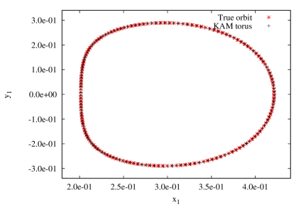
Figure 3: On the left, the norms (in log scale) of the generating functions $\chi_{2}^{(r)}$ introduced by the algorithms for the construction of the normal form for a KAM torus: the one above refers to the algorithm without fixing the frequencies and the one below to the algorithm with the translation for keeping the frequency vector fixed as $\tilde{{\bm{\omega}}}$. On the right, the Poincaré sections of the true orbit (in red) and of the orbit with initial conditions on the KAM torus constructed with our algorithm (in black).

At this level, we start to iterate the algorithm for the construction of the normal form for a KAM torus, in a first version that is without introducing any other translation to target the frequencies of the quasi-periodic motion characterizing the wanted invariant manifold. This is equivalent to construct one of the intermediate tori between the elliptic torus and the true orbit. By using the Newton method described at the end of the previous Section 3, this computational procedure can converge to values $(\tilde{I}_{1}\,,\,\tilde{I}_{2})$, that enter into the definition (39) of the initial translation $\chi({\bm{q}})$. These values are such that the relative error between the frequency of the approximated KAM torus ${\bm{\omega}}^{(r)}$ and the numerical one $\tilde{{\bm{\omega}}}$ is less than $10^{-3}$. Then, we apply one last time the classical KAM algorithm, i.e., with the addition of a translation at each normalization step in order to keep the frequency fixed. In Figure 3, we plot the norms of the generating functions $\chi_{2}^{(r)}$ for both the normalization algorithms, the one without any other translation apart from the initial one $\chi({\bm{q}})$ defined in (39) and the one enqueued with the translation ${\bm{\xi}}^{(r)}\cdot{\bm{q}}$ at each step $r$ for aiming at the wanted frequency vector $\tilde{{\bm{\omega}}}$. We can observe in both cases a slow decrease of the norm and, in particular, that we have an improvement in iterating the algorithm at fixed frequency only subsequently, when the perturbation has been considerably reduced. Being the convergence rate quite slow, it is not so rare to encounter high order resonances that, even if they do not compromise the convergence, have an evident impact in the norms of the generating functions, appearing as small and sudden peaks. This is the reason why we have iterated the first algorithm just half the steps in order to reduce the danger of falling in a resonant region because of the random variation of the sequence ${\bm{\omega}}^{(r)}$. Such a problem is not truly related to the non-resonance properties of the frequency vector $\tilde{{\bm{\omega}}}$.

In the same way as before, we can evaluate the composition of all the transformations of coordinates introduced into the framework of the previous Section 3, with the aim of constructing a well defined sequence of Hamiltonians, that in principle should converge to the Kolmogorov normal form (43). Therefore, we can consider the initial conditions $({\bm{\xi}}(0),{\bm{\eta}}(0))$ which corresponds to a point $({{\bm{p}}}(0),{{\bm{q}}}(0))=({{\bm{0}}},{{\bm{0}}})$ belonging to the torus that we have built and is expected to be invariant with a very good approximation. Hence, we integrate numerically the equation of motions starting from the initial conditions $({\bm{\xi}}(0),{\bm{\eta}}(0))$ and we can plot the corresponding Poincaré sections with respect to the $(x_{1}\,,\,y_{1})$–plane. In the right panel of Figure 3, we compare the Poincaré sections of this orbit with those of the true secular orbit, obtaining an excellent superposition. Such a comparison confirms that the true orbit should lie very close to a KAM torus, because it can be approximated very well by the solution we have constructed using a normal form technique.

4.2 Rigorous results

By comparing the two plots in the left panels of Figures 2–3, one can appreciate that the decrease of the norms in the final Kolmogorov algorithm is way slower and more irregular with respect to the case of the elliptic torus. This remark makes doubtful the convergence to a Kolmogorov normal form for what concerns the sequence of Hamiltonians introduced in subsection 3.2. In this framework, the most convincing argument is definitely provided by a rigorous computer-assisted proof, that we will discuss in the following.

According to the strategy designed in [9], it is convenient to preliminarly perform a large enough number of normalization steps constructing the Kolmogorov normal form. This is made with the purpose of reducing the size of the perturbative terms so much that it is possible to apply a suitable version of the KAM theorem. In practice, the perturbation is made smaller by applying a procedure where a couple of different stages can be distinguished. First, the expansions of the generating functions $X^{(r)}$, ${\bm{\xi}}^{(r)}\cdot{\bm{q}}$ and $\chi_{2}^{(r)}$ are explicitly computed when the index $r$ of the normalization step is running from $1$ to $R_{\rm I}\,$; then, just the estimates of the norms of terms up to order $\varepsilon^{R_{\rm II}}$ are iterated, by avoiding the calculation of their cumbersome expansions if they are $\mathcal{O}(\varepsilon^{r})$ with $R_{\rm I}<r\leq R_{\rm II}\,$. All the terms appearing in a Hamiltonian $\mathcal{K}^{(r-1)}$ satisfy suitable inequalities that involve a finite number of quantities in the definition of the upper bounds, being the latter ones collected in a set $\mathcal{S}^{(r-1)}$ of the type described in (46). Appendix A includes the recursive formulæ allowing to properly define the values of the elements that belong to the set $\mathcal{S}^{(r)}$ and provide the upper bounds for the terms making part of Hamiltonian $\mathcal{K}^{(r)}$. In particular, the way to iterate the estimates of the norms of the generating functions is fully explained in such an appendix. The number $R_{\rm I}$ of the first normalization steps that are performed by explicitly computing the expansion of the generating functions must be large enough, in order to subsequently iterate the estimates in a so successful way to reduce the size of the perturbation as much as needed.

Figure 4: Estimates of the norms (in semi-log scale) of the generating function $\chi_{2}$. On the right, the zoom on the first 500 normalization steps.

For our purposes, we have seen that it is enough to set $R_{\rm I}=60$ and to represent the estimates of the norms of terms up to order $\varepsilon^{R_{\rm II}}$ with $R_{\rm II}=10000$. The plots of the estimates of the norm of $\chi_{2}^{(r)}$ are reported in Figure 4 and confirm the slow but regular reduction of the perturbation. Indeed, the plot in the right box of such a figure highlights that the decrease is steeper up to the step $60$, i.e., when an explicit computation of the generating function is performed; then, we have a sudden leap, due to the transition to the regime of the pure iteration of the estimates; thereafter, a periodic and increasingly small jump is noticeable until the decrease stabilizes to a flatter but nearly constant slope. As it is discussed also in the explanatory document included in the software package allowing to implement such a kind of computer-assisted proofs (see [25]), it is an important achievement when the behavior of the norms of the generating functions looks similar to that depicted in Figure 4. In fact, this ensures that the existence of quasi-periodic motions of frequency vector $\tilde{{\bm{\omega}}}$ and invariant with respect to the Kolmogorov normal form (43) can be rigorously proved, by eventually increasing the index of the final normalization step $R_{\rm II}\,$. In the case of the model we are studying, the perturbative terms appearing in the expansion of the Hamiltonian $\mathcal{K}^{(10000)}$ are so small that the computer-assisted proof can be successfully completed by applying the KAM theorem in the version described in [37]. Performing the first $R_{\rm I}=60$ normalization steps so as to explicitly determine the expansion of all the corresponding generating functions requires nearly 7 hours on the same computer whose CPU is described in footnote${\ref{nota:CPU-specs}}\atop{\phantom{1}}$; moreover, about two additional hours of CPU-time are needed by the iteration of the estimates for the norms of terms up to order $\varepsilon^{R_{\rm II}}$ with $R_{\rm II}=10000$. Of course, the larger amount of time that is requested by the explicit construction of the normal form can be easily explained because of the huge number of terms to manipulate. This is also due to our decision to represent in the expansions of the finite sequence of Hamiltonians $\big{\{}\mathcal{K}^{(r)}\big{\}}_{r=0}^{60}$ all the terms having up to degree $8$ in the actions, while the maximal trigonometrical degree has been fixed to $2R_{\rm I}=120$. Such a truncation rule on the actions is in agreement with the limits we have adopted during the the computation of the Hamiltonians $\mathcal{H}^{(0)},\ldots,\,\mathcal{H}^{(17)}$, that has been made according to the algorithm described in subsection 3.2. These preliminary expansions have been basic to produce the semi-analytical results already discussed in the previous subsection 4.1.

The result we have obtained thanks to a rigorous proof can be summarized as follows.

Theorem 4.1 (Computer-assisted)

Let us consider the Hamiltonian $\mathcal{K}^{(0)}=\mathcal{H}^{(17)}$ whose expansion is written in (38) that has been obtained by following the procedure described in sections 3.1-3.2 and by truncating all the expansions up to degree $8$ in the actions and to the trigonometrical degree $72$ in the angles. Let $\tilde{{\bm{\omega}}}\in\mathbb{R}^{2}$ be such that

$${\tilde{\omega}_{1}}$$

(47)

and it satisfies the Diophantine inequality

$$|{\bm{k}}\cdot\tilde{{\bm{\omega}}}|\geq\frac{\gamma}{|{\bm{k}}|}\qquad\forall\ {\bm{k}}\in\mathbb{Z}^{2}\setminus\{{\bm{0}}\}$$ (48)

with $\gamma=2.094439\times 10^{-4}$.

Therefore, there exists an analytic canonical transformation conjugating $\mathcal{H}^{(17)}$ to the Kolmogorov normal form $\mathcal{K}^{(\infty)}$, which is written in (43). It is such that the torus $\{{\bm{p}}={\bm{0}},{\bm{q}}\in\mathbb{T}^{2}\}$ is invariant and travel led by quasi-periodic motions whose corresponding angular velocity vector is equal to $\tilde{{\bm{\omega}}}$.

Let us recall that the dynamical stability of our planetary model is expected to follow from the proof of existence of an invariant torus close to the true orbit. Indeed, two possible approaches can be successfully adopted in this framework. By following the strategy designed in [26], one could prove the existence of a KAM torus that encloses the true orbit in the Poincaré sections represented in the first panel of Figure 1. Since the Hamiltonian secular model has two degrees of freedom, the constant energy surface is 3D and so 2D invariant tori that certainly include the initial conditions are able to ensure a perpetual topological confinement of the true orbit. Otherwise, a more general approach (that is valid also for Hamiltonian systems having more than two degrees of freedom) can be applied so to lead to the effective stability concept: in the neighborhood of the KAM torus, a Birkhoff normal form can be constructed and complemented with the classical estimates à la Nekhoroshev (see [32]). This allows to prove that the time needed to eventually escape from a small enough region surrounding the KAM torus can largely exceed the expected life-time of such a system. Such an approach can be used to show the effective stability of Hamiltonian planetary models (see [14] and [16]). Both these approaches would require a demanding effort for their actual implementations, that we will avoid because we believe that a complete proof of the stability of the secular system goes beyond the aims of the present work.

4.3 Comparisons between the dynamics for the complete planetary model and the secular one

From a more astronomical point of view, it is natural to raise the following question: how far is reality from the secular Hamiltonian model we are considering? There are different possible answers to such a question. In order to give some insights, it is natural to compare the solutions for the secular model with those related to the complete planetary system introduced at the very beginning in formula (1). Such a comparison can be performed just for the motion laws that can be observed in both these dynamical systems, these obviously refer to the secular variables.

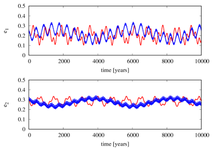
Figure 5: Comparisons between the results provided by the numerical integrations of the complete planetary system and the secular one (in blue and in red, respectively). In the left box, the behavior of the difference of the arguments of the pericenters is plotted as a function of time. On the right, the temporal evolutions of the eccentricities are reported: the plot above [below] refers to $\upsilon$ And c [$\upsilon$ And d, resp.].

On the one hand, we have produced the numerical integrations of the equations of motion related to the complete planetary Hamiltonian (1), by using the symplectic integrator of type $\mathcal{S}\mathcal{B}\mathcal{A}\mathcal{B}_{3}\,$, which is described in [23]. On the other hand, the secular Hamiltonian model (11) has been integrated by using the RK4 method; let us here recall that the comparisons would not have changed significantly if we would have adopted the semi-analytic computations described at the end of subsection 4.1. This is due to the fact that the plots produced by applying the latter two methods superpose in a practically indistinguishable way. Of course, the numerical integrations have been started from two sets of initial conditions that are coherent between them because both of them correspond to the same values of the orbital elements, that are reported in Table 1. Figure 5 includes those results that can be directly compared. It clearly shows that the secular model is able to substantially capture some of the main dynamical features of the complete one: the quasi-periodicity of the motions and the amplitudes of all the plotted quantities, that are the eccentricities of the two planets and the difference of the arguments of their pericenters. However, the comparisons that are reported in Figure 5 are not satisfactory at all for what concerns the fundamental angular velocities that generate all the quasi-periodic motions. Indeed, the periods look rather different. This is particularly true for what concerns the component giving the slow modulation that can be easily observed in the orbital laws induced by the flow of the complete planetary Hamiltonian (1): none of the Fourier harmonics composing the motion related to the secular model looks to play the same role. We stress that the agreement is much worse with respect to the one we get for the Sun–Jupiter–Saturn system. In that case, the same kind of comparisons between the complete planetary Hamiltonian and the secular one (still calculated at order two in the masses) showed a minimal discrepancy, because the relative errors on the angular velocities of the perihelion arguments of Jupiter and Saturn are about 0.1% and 1.3%, respectively (see at the end of Section 2 of [26]).

5 Conclusions and perspectives

Computer-assisted algorithms based on the construction of the Kolmogorov normal form can provide very good performances when a toy model is considered. For instance, in [9] the Authors rigorously prove the existence of invariant tori for values of the perturbing terms that are relatively close to the expected breakdown threshold. When applied to a model that is more similar to a system of physical interest though, the same approach is able to prove the KAM theorem only in situations that are still rather far from the edge (see [38]). Therefore, the results described in the present paper can be considered astonishingly good, considering the adherence of the model to the physical problem. On one hand, the $\upsilon$ Andromedæ planetary system is considered to be much more perturbed with respect to the Sun–Jupiter–Saturn one studied, for example, in [26]. On the other hand, for both these three-body problems, the computer-assisted proofs can produce the same result when they are used at their best: they ensure the existence of invariant tori into the framework of a realistic secular model that is calculated at order two in the masses, with the purpose to well approximate their planetary dynamics. A key ingredient that we introduce in the present work is the construction of a preliminary normal form that allows to approximate a lower dimensional elliptic invariant torus. It should be noted that few details introduced in the approach presented in this work lead to some simplifications. For instance, we have considered the initial conditions reported in Table 1 that are expected to be the most robust among those compatible with the observational data reported in [28]. Moreover, the proof of convergence relates only to the final normalization algorithm, instead of the whole sequence of algorithms applied. It would be desirable to further refine the techniques adopted in the context of this kind of computer-assisted proofs, in order to apply them to realistic models without any extra simplification, as it already happens for toy models (see [11]).

In our view, the interest of our work goes beyond the rigorous mathematical proofs ensuring the existence of invariant tori. The adaptation of the constructive algorithm to the case of librational tori emphasizes their role in stabilizing the planetary orbits. This is strictly related to the criterion of robustness that allows us to make selections among the initial conditions that are compatible with the observations. Such a criterion will be explained in a forthcoming publication and it will require a further extension to the systems in Mean Motion Resonance (MMR). For such a reason, we stress the importance of adapting our approach to MMR planetary models so as to combine the constructions of the normal forms for both elliptic and KAM tori. In the framework of MMR systems, the librational orbits are more complicated with respect to those considered in the present paper, but the effectiveness of the computational procedure constructing an average model at order two in the masses has already been shown (see [34]).

The main advantage of normal form methods is that they allow to describe the dynamics in a region of the phase space, instead of analyzing one trajectory at a time, thus obtaining a result in a set of zero measure. In particular, in this work we have designed an approach based on a preliminary construction of the elliptic tori, before studying the librational orbits in their neighborhood. Indeed, the secular model here introduced shows some discrepancies between the semi-analytical results and the motions generated by the complete planetary Hamiltonian (as shown in Figure 5). A better agreement with the numerical solutions can be achieved by extending the normal form approach from the secular Hamiltonian to the complete one. In other words, we should apply the same adaption of the constructive algorithm that was successfully implemented by passing from [26] to [27] in the case of the Sun–Jupiter–Saturn system.

The characterization of the three dimensional architecture of extrasolar planetary systems is one of the very exciting problems that is currently investigated in Dynamical Astronomy. It has been studied within the framework of both complete and secular planetary Hamiltonians (see, e.g., [30], [24] and [40]). In [39], some of the Authors of this article introduced a reverse approach based on KAM theory: values of the mutual inclinations are considered to be acceptable if the subsequent construction of the Kolmogorov normal form is convergent. The effectiveness of that method was limited to extrasolar systems hosting planets with very moderate eccentricities (i.e., smaller than $0.1$). The original motivation of the present work was aiming to overcome this artificial constraint due to the technique adopted in [39]. In this respect, the present work is certainly successful, because the average eccentricity for stable planetary orbits is about $0.3$ in the case of the model we considered here for studying the $\upsilon$ Andromedæ system. In a near future, we plan to restart the explorations of the 3D architecture of extrasolar planetary systems, with the prescription of the KAM stability of those models. Of course, this will be made by exporting the new strategy introduced here, namely by combining the constructions of the normal forms for both elliptic tori and KAM ones.

Data Availability

The data that support the findings of this study are available from the corresponding author, C. C., upon reasonable request.

Acknowledgments

This work was partially supported by the MIUR-PRIN project 20178CJA2B – “New Frontiers of Celestial Mechanics: theory and Applications”, the “Beyond Borders” program of the University of Rome Tor Vergata through the project ASTRID (CUP E84I19002250005), the “Progetto Giovani 2019” program of the National Group of Mathematical Physics (GNFM–INdAM) and the ASI Contract n. 2018-25-HH.0 (Scientific Activities for JUICE, C/D phase). The authors acknowledge also the MIUR Excellence Department Project awarded to the Department of Mathematics of the University of Rome “Tor Vergata” (CUP E83C18000100006).

Appendix A Computer-assisted proof of the existence of KAM tori: technicalities

In this appendix we describe how to iteratively define the terms making part of $\mathcal{S}^{(r)}$, as it is defined in (46). Such an iterative scheme of estimates is effectively implemented in a software package dealing with the computer-assisted proof whose result is discussed in section 4.2. Let us recall that this package is publicly available from the web [25] and it subdivides the expansions in Hamiltonian terms according to slightly different definitions with respect to those adopted in subsection 3.2. This is made in order to improve the results obtained by performing the computer-assisted proof. Indeed, since the very beginning (i.e., when the normalization step $r=0$), the codes in the already mentioned software package [25] consider expansions of Hamiltonians of the following type:

$$\mathcal{K}^{(r)}=E^{(r)}+\tilde{{\bm{\omega}}}\cdot{\bm{p}}+\sum_{s\geq 0}\sum_{\ell\geq 2}f_{\ell}^{(r,s)}({\bm{p}},{\bm{q}})+\sum_{s\geq r+1}\sum_{\ell=0}^{1}f_{\ell}^{(r,s)}({\bm{p}},{\bm{q}})\ ,$$ (49)

where $f_{\ell}^{(r,s)}\in{\mathfrak{P}}_{\ell\,,\,2s}$ $\forall\ \ell,\,s$. A generic function $g$ belongs to the class of functions ${\mathfrak{P}}_{\ell\,,\,2s}$ if its Taylor–Fourier expansion is such that

$$g({\bm{p}},{\bm{q}})=\sum_{{j_{1}+\ldots+j_{n}=\ell}}\ \sum_{\max_{i=1,\ldots,n}|k_{i}|\leq 2s}\,{\bm{p}}^{{\bm{j}}}\big{[}c_{{\bm{j}},{\bm{k}}}\cos({{\bm{k}}}\cdot{{\bm{q}}})+d_{{\bm{j}},{\bm{k}}}\sin({{\bm{k}}}\cdot{{\bm{q}}})\big{]}\ ,$$ (50)

where $n$ denotes the number of degrees of freedom and the coefficients $c_{{\bm{j}},{\bm{k}}}\,,\,d_{{\bm{j}},{\bm{k}}}\in\mathbb{R}$; in the previous formula, we have also adopted the multi-index notation, i.e., ${\bm{p}}^{{\bm{j}}}=p_{1}^{j_{1}}\cdot\ldots\cdot p_{n}^{j_{n}}$. This means that the only difference with respect to to the expansions described during the discussion of the formal algorithm in subsection 3.2 is due to the fact that here we consider the $\ell_{\infty}$-norm of the Fourier harmonic ${\bm{k}}$ in order to make the separation with respect to different classes of function, instead of the $\ell_{1}$-norm $|{\bm{k}}|$, that has also been called the trigonometrical degree corresponding to ${\bm{k}}$. Let us recall that the functional norm whose corresponding values for some generating functions are reported in the plots of Figures 2–4 is defined in such a way that

$$\|g\|=\sum_{{j_{1}+\ldots+j_{n}=\ell}}\ \sum_{\max_{i=1,\ldots,n}|k_{i}|\leq 2s}\,\left(\big{|}c_{{\bm{j}},{\bm{k}}}\big{|}+\big{|}d_{{\bm{j}},{\bm{k}}}\big{|}\right)$$

(see the corresponding footnote${\ref{nota:def-norma}}\atop{\phantom{1}}$ in subsection 3.3). Being the transformations of coordinates defined by the Lie series, the estimates of the functional norm $\|\cdot\|$ that are needed can be summarized by the following statement.

Lemma A.1

Let $g$ be a generic function belonging to the class of functions ${\mathfrak{P}}_{\ell\,,\,sK}\,$, for some non-negative integers $\ell$ and $s$, with $K\in\mathbb{Z}^{+}$. Let us consider the Lie series $\exp\mathcal{L}_{\chi_{1}^{(r)}}g$ and $\exp\mathcal{L}_{\chi_{2}^{(r)}}g$, where the generating functions are such that $\chi_{1}^{(r)}=X^{(r)}+{\bm{\xi}}^{(r)}\cdot{\bm{q}}$, being $X^{(r)}\in{\mathfrak{P}}_{0\,,\,rK}\,$, ${\bm{\xi}}^{(r)}\in\mathbb{R}^{n}$, and $\chi_{2}^{(r)}\in{\mathfrak{P}}_{1\,,\,rK}\,$. Therefore, the following estimates hold true for the summands appearing in the expansions of those Lie series:

$$\left\|\frac{1}{j!}\mathcal{L}_{\chi_{1}^{(r)}}^{j}g\right\|\leq \binom{\ell}{j}\left(\max_{i}\left\{\left\|\frac{\partial X^{(r)}}{\partial q_{i}}\right\|\right\}+\max_{i}\left\{\left|\xi_{i}^{(r)}\right|\right\}\right)^{j}\|g\|\ ,$$ (51)

$$\left\|\frac{1}{j!}\mathcal{L}_{\chi_{2}^{(r)}}^{j}g\right\|\leq \frac{1}{j!}\prod_{i=1}^{j}\left[\ell\max_{i}\left\{\left\|\frac{\partial\chi_{2}^{(r)}}{\partial q_{i}}\right\|\right\}+K(s+(i-1)r)\max_{i}\left\{\left\|\frac{\partial\chi_{2}^{(r)}}{\partial p_{i}}\right\|\right\}\right]\|g\|\ .$$ (52)

Since the proof can be easily reconstructed by applying repeatedly the definition of the Poisson brackets, it is omitted. Let us recall that we have always adopted $K=2$ for all the computations described in Sections 3 and 4.

The statement of lemma A.1 makes evident that we need to bound the derivatives of the generating functions, in such a way to determine four majorants $\mathcal{G}_{11}^{(r)}$, $\mathcal{G}_{12}^{(r)}$, $\mathcal{G}_{21}^{(r)}$ and $\mathcal{G}_{22}^{(r)}$ satisfying the inequalities $\max_{i}\|\partial X^{(r)}/\partial q_{i}\|\leq\mathcal{G}_{11}^{(r)}$, $\max_{i}|\xi_{i}^{(r)}|\leq\mathcal{G}_{12}^{(r)}$, $\max_{i}\|\partial\chi_{2}^{(r)}/\partial q_{i}\|\leq\mathcal{G}_{21}^{(r)}$ and $\max_{i}\|\partial\chi_{2}^{(r)}/\partial p_{i}\|\leq\mathcal{G}_{22}^{(r)}$ at the generic normalization step $r$. When it is not possible to explicitly calculate those derivatives, because the expansions of $\chi_{1}^{(r)}$ and $\chi_{2}^{(r)}$ are unknown, it is convenient to define their upper bounds as follows:

$$\mathcal{G}_{11}^{(r)} \leq 2r\left(\min_{0<\max_{i}|k_{i}|\leq 2r}|{\bm{k}}\cdot{\bm{\omega}}|\right)^{-1}\mathcal{F}_{0}^{(r-1,r)}\ ,\quad\mathcal{G}_{12}^{(r)}\leq(m^{(r)})^{-1}\langle\mathcal{F}_{1}^{(r-1,r)}\rangle\ ,$$ (53)

$$\mathcal{G}_{21}^{(r)} \leq 2r\left(\min_{0<\max_{i}|k_{i}|\leq 2r}|{\bm{k}}\cdot{\bm{\omega}}|\right)^{-1}\mathcal{F}_{1}^{(r-1,r)}\ ,\quad\mathcal{G}_{22}^{(r)}\leq\left(\min_{0<\max_{i}|k_{i}|\leq 2r}|{\bm{k}}\cdot{\bm{\omega}}|\right)^{-1}\mathcal{F}_{1}^{(r-1,r)}\ ,$$ (54)

being $\mathcal{F}_{\ell}^{(r,s)}$ an estimate of the norm of the generic term $f_{\ell}^{(r,s)}$ and $m^{(r)}$ is such that $|C^{(r)}\cdot v|\geq m^{(r)}|v|\ \forall\ v\in\mathbb{R}^{n}$, where $C^{(r)}$ is the matrix defined by the equation $\frac{1}{2}C^{(r)}{\bm{p}}\cdot{\bm{p}}=\sum_{s=0}^{r}\langle f_{2}^{(r,s)}\rangle$. The estimates in lemma A.1, combined with the formulæ for the re-definitions of the Hamiltonian terms in (36) and (37), provide the following outcomes:

$${\hat{\mathcal{F}}_{\ell-j}^{(r,jr+s)}}$$

(55)

(after having initially set $\hat{\mathcal{F}}_{\ell}^{(r,s)}=\mathcal{F}_{\ell}^{(r-1,s)}$ $\forall\ \ell\geq 0,\ s\geq 0$) and

$${\mathcal{F}_{\ell}^{(r,jr+s)}}$$

(56)

(after having initially set $\mathcal{F}_{\ell}^{(r,s)}=\hat{\mathcal{F}}_{\ell}^{(r,s)}$ $\forall\ \ell\geq 0,\ s\geq 0$). Of course, after having completed all the re-definitions prescribed by formula (55), we have to impose that $E^{(r)}=E^{(r-1)}+\hat{\mathcal{F}}_{0}^{(r,r)}$ and $\hat{\mathcal{F}}_{0}^{(r,r)}=0$; analogously, at the end of the re-definitions (56), we have to set $\hat{\mathcal{F}}_{1}^{(r,r)}=0$. This is made in order to update the energy value that at the end of the procedure will correspond to that of the invariant KAM torus and to take into account of the homological equations (29), (30) and (42). Furthermore, the estimate ensuring that the non-degeneracy condition is satisfied has to be updated thanks to the following redefinition:

$$m^{(r+1)}=m^{(r)}-2\mathcal{F}_{2}^{(r,r)}.$$ (57)

Let us emphasize that all the estimates (53)–(57) for the quantities $\mathcal{G}_{11}^{(s)}$, $\mathcal{G}_{12}^{(s)}$, $\mathcal{G}_{21}^{(s)}$, $\mathcal{G}_{22}^{(s)}$, $\hat{\mathcal{F}}_{\ell}^{(r,s)}$, $\mathcal{F}_{\ell}^{(r,s)}$ and $m^{(s)}$ are used just when $R_{\rm I}<s\leq R_{\rm II}$, while the estimates are made directly from the expansions of the (generating) functions that are computed explicitly for all $0\leq s\leq R_{\rm I}$. Of course, this is made in order to take advantage as much as possible from the explicit computations. We stress that Figure 4 actually includes the plots of the finite sequence of values $\mathcal{G}_{22}^{(r)}$ (as a function of the normalization step $r$), that are computed exactly as it has been explained in the present appendix.

In order to complete the iterative definition of the set $\mathcal{S}^{(r)}$, we have to determine the three parameters that appear in formula (46) and are ruling the decay of the infinite tail of terms making part of the expansions of the Hamiltonian $\mathcal{H}^{(r)}$; they are $\mathcal{E}_{r}\,$, $a_{r}$ and $\zeta_{r}\,$. These final settings are omitted because they can be easily found in subsection 3.2.3 of [38].

References

- [1] V.I. Arnold: Proof of a theorem of A. N. Kolmogorov on the invariance of quasi-periodic motions under small perturbations of the Hamiltonian, Usp. Mat. Nauk, 18, 13 (1963); Russ. Math. Surv., 18, 9 (1963).
- [2] C. Beaugé, S. Ferraz-Mello and T.A. Michtchenko: Multi-planet extrasolar systems – detection and dynamics, Research in Astron. and Astroph., 12, 1044–1080 (2012).
- [3] R.P. Butler, G.W. Marcy, D.A. Fischer, T.M. Brown, A.R. Contos, S.G. Korzennik, P. Nisenson and R.W. Noyes: Evidence for Multiple Companions to Andromedæ, Astroph. Jour., 526, 916–927 (1999).
- [4] E.I. Chiang, S. Tabachnik and S. Tremaine: Apsidal Alignment in Andromedæ, Astron. Jour., 122, 1607–1615 (2001).
- [5] C. Caracciolo: Normal form for lower dimensional elliptic tori: convergence of a constructive algorithm, submitted (2021).
- [6] C. Caracciolo and U. Locatelli: Computer-assisted estimates for Birkhoff normal forms, J. of Comput. Dyn., 7, 425–460 (2020).
- [7] C. Caracciolo and U. Locatelli: Elliptic tori in FPU non-linear chains with a small number of nodes, Commun. Nonlinear Sc. Numer. Simulat., 97, 105759 (2021).
- [8] A. Celletti and L. Chierchia: KAM stability and Celestial Mechanics, Memoirs of AMS, 187, n. 878 (2007).
- [9] A. Celletti, A. Giorgilli and U. Locatelli: Improved estimates on the existence of invariant tori for Hamiltonian systems, Nonlinearity, 13, 397–412 (2000).
- [10] R. Deitrick, R. Barnes, B.E. McArthur, T.R. Quinn, R. Luger, A. Antonsen and G.F. Benedict: The Three-Dimensional Architecture of the Andromedæ, Astroph. Jour., 798:46 (2015).
- [11] J.-Ll. Figueras, A. Haro and A. Luque: Rigorous computer-assisted application of KAM theory: a modern approach, Found. Comput. Math., 17, 1123–1193 (2017).
- [12] L. Duriez: Poisson’s theorem in heliocentric variables, Astron. & Astroph., 68, 199–216 (1978).
- [13] F. Gabern, A. Jorba and U. Locatelli: On the construction of the Kolmogorov normal form for the Trojan asteroids, Nonlinearity, 18, 1705–1734 (2005).
- [14] A. Giorgilli, U. Locatelli and M. Sansottera: Kolmogorov and Nekhoroshev theory for the problem of three bodies, Cel. Mech. & Dyn. Astr., 104, 159–173 (2009).
- [15] A. Giorgilli, U. Locatelli and M. Sansottera: On the convergence of an algorithm constructing the normal form for lower dimensional elliptic tori in planetary systems, Cel. Mech. & Dyn. Astr., 119, 397–424 (2014).
- [16] A. Giorgilli, U. Locatelli and M. Sansottera: Secular dynamics of a planar model of the Sun-Jupiter-Saturn-Uranus system; effective stability in the light of Kolmogorov and Nekhoroshev theories, Regular and Chaotic Dynamics, 22, 54–77 (2017).
- [17] A. Giorgilli and M. Sansottera: Methods of algebraic manipulation in perturbation theory, in “Chaos, Diffusion and Non-integrability in Hamiltonian Systems — Applications to Astronomy”, Proceedings of the Third La Plata International School on Astronomy and Geophysics, P.M. Cincotta, C.M. Giordano and C. Efthymiopoulos eds., Universidad Nacional de La Plata and Asociación Argentina de Astronomía Publishers, La Plata (2012).
- [18] S. Kim and S. Ostlund: Simultaneous rational approximations in the study of dynamical systems, Physical Review A, 34, 3426–3434 (1986).
- [19] A.N. Kolmogorov: Preservation of conditionally periodic movements with small change in the Hamilton function, Dokl. Akad. Nauk SSSR, 98, 527 (1954). Engl. transl. in: Los Alamos Scientific Laboratory translation LA-TR-71-67; reprinted in: Lecture Notes in Physics, 93.
- [20] Laskar J.: Les variables de Poincaré et le développement de la fonction perturbatrice in “Groupe de travail sur la lecture des Méthodes Nouvelles de la Mécanique Céleste” Notes scientifiques et techniques du Bureau des Longitudes S 026, Paris (1989).
- [21] J. Laskar: Frequency Map analysis and quasi periodic decompositions, in Benest, D., Froeschlé, C. and Lega E. (eds.): Hamiltonian systems and Fourier analysis, Taylor and Francis (2003).
- [22] J. Laskar and A.C. Petit: AMD-stability and the classification of planetary systems, Astron. & Astroph., 605, A72 (2017).
- [23] J. Laskar and P. Robutel: High order symplectic integrators for perturbed Hamiltonian systems, Cel. Mech. & Dyn. Astr., 80, 39-62 (2001).
- [24] A.-S. Libert and K. Tsiganis: Kozai resonance in extrasolar systems, Astron. & Astroph., 493, 677–686 (2009).
- [25] U. Locatelli: CAP4KAM2D: Computer-Assisted Proofs For demonstrating the existence of 2-Dimensional KAM tori, Mendeley Data, V1, doi: 10.17632/jdx22ysh2s.1 (2021); publicly available at the web address https://data.mendeley.com/datasets/jdx22ysh2s/1
- [26] U. Locatelli and A. Giorgilli: Invariant tori in the secular motions of the three-body planetary systems, Cel. Mech. & Dyn. Astr., 78, 47–74 (2000).
- [27] U. Locatelli and A. Giorgilli: Invariant tori in the Sun-Jupiter-Saturn system, DCDS-B, 7, 377–398 (2007).
- [28] B.E. McArthur, G.F. Benedict, R. Barnes, E. Martioli, S. Korzennik, E. Nelan and R.P. Butler: New observational constraints on the Andromedæ system with data from the Hubble Space telescope and Hobby-Eberly telescope, Astroph. Jour., 715, 1203–1220 (2010).
- [29] R.S. MacKay and J. Stark: Locally most robust circles and boundary circles for area–preserving maps, Nonlinearity, 5 867–888 (1992).
- [30] T.A. Michtchenko, S. Ferraz-Mello and C. Beaugé: Modeling the 3-D secular planetary three-body problem, Icarus, 181, 555–571 (2006).
- [31] T.A. Michtchenko and R. Malhotra: Secular Dynamics of the Three-Body Problem: Application to the Andromedæ Planetary System, Icarus, 168, 237–248 (2004).
- [32] A. Morbidelli and A. Giorgilli: Superexponential stability of KAM tori, J. Stat. Phys., 78, 1607–1617 (1995).
- [33] J. Moser: On invariant curves of area-preserving mappings of an annulus, Nachr. Akad. Wiss. Gött,. II Math. Phys. Kl 1962, 1–20 (1962).
- [34] M. Sansottera and A.-S. Libert: Resonant Laplace-Lagrange theory for extrasolar systems in mean-motion resonance, Cel. Mech. & Dyn. Astr., 131, 38 (2019).
- [35] M. Sansottera, U. Locatelli and A. Giorgilli: A semi-analytic algorithm for constructing lower dimensional elliptic tori in planetary systems , Cel. Mech. & Dyn. Astr., 111, 337–361 (2011).
- [36] M. Sansottera, U. Locatelli and A. Giorgilli: On the stability of the secular evolution of the planar Sun-Jupiter-Saturn-Uranus system, Math. Comp. Sim., 88, 1–14 (2013).
- [37] L. Stefanelli and U. Locatelli: Kolmogorov’s normal form for equations of motion with dissipative effects, DCDS-B, 17, 2561–2593 (2012).
- [38] L. Valvo and U. Locatelli: Hamiltonian Control of Magnetic Field Lines: Computer Assisted Results Proving the Existence of KAM Barriers, preprint (2021); publicly available at the webpage https://arxiv.org/abs/2101.07785
- [39] M. Volpi, U. Locatelli and M. Sansottera: A reverse KAM method to estimate unknown mutual inclinations in exoplanetary systems, Celest. Mech. Dyn. Astr., 130:36 (2018).
- [40] M. Volpi, A. Roisin and A.-S. Libert: On the 3D secular dynamics of radial-velocity-detected planetary systems, Astron. & Astroph., 626, A74 (2019).