Efficient Out-of-Distribution Detection Using Latent Space of $\beta$-VAE for Cyber-Physical Systems

Abstract.

Deep Neural Networks are actively being used in the design of autonomous Cyber-Physical Systems (CPSs). The advantage of these models is their ability to handle high-dimensional state-space and learn compact surrogate representations of the operational state spaces. However, the problem is that the sampled observations used for training the model may never cover the entire state space of the physical environment, and as a result, the system will likely operate in conditions that do not belong to the training distribution. These conditions that do not belong to training distribution are referred to as Out-of-Distribution (OOD). Detecting OOD conditions at runtime is critical for the safety of CPS. In addition, it is also desirable to identify the context or the feature(s) that are the source of OOD to select an appropriate control action to mitigate the consequences that may arise because of the OOD condition. In this paper, we study this problem as a multi-labeled time series OOD detection problem over images, where the OOD is defined both sequentially across short time windows (change points) as well as across the training data distribution. A common approach to solving this problem is the use of multi-chained one-class classifiers. However, this approach is expensive for CPSs that have limited computational resources and require short inference times. Our contribution is an approach to design and train a single $\beta$-Variational Autoencoder detector with a partially disentangled latent space sensitive to variations in image features. We use the feature sensitive latent variables in the latent space to detect OOD images and identify the most likely feature(s) responsible for the OOD. We demonstrate our approach using an Autonomous Vehicle in the CARLA simulator and a real-world automotive dataset called nuImages.

1. Introduction

Significant advances in Artificial Intelligence (AI) and Machine Learning (ML) are enabling dramatic, unprecedented capabilities in all spheres of human life, including cps. The fundamental advantage of AI methods is their ability to handle high-dimensional state-space and learn decision procedures or control algorithms from data rather than models. This is because high-dimensional real-world state spaces are complex and intractable for mathematical modeling and analysis. As such it is common to find AI components like dnn in real-world cps such as autonomous cars  (Pomerleau, 1989; Bojarski et al., 2016), autonomous underwater vehicles  (Eski and Yildirim, 2014), and homecare robots  (Ko et al., 2017). However, there is still a gap in the safety and assurance of AI-driven cps as shown by well known incidents in recent past  (Vlasic and Boudette, 2016; Kohli and Chadha, 2019). The technical debt is fundamentally in the black-box nature of AI components, which hinders the use of classical software testing strategies (e.g., code coverage, function coverage). There is research progress on testing  (Pei et al., 2017; Tian et al., 2018), however, wide-spread applicability remains questionable. The problem is exacerbated due to the way the systems are being designed.

The Safety Conundrum: cps design flows focus on designing a system $S$ that satisfies some requirements $R$ in an environment $E$. During the design process, the developer selects component models, each including a parameter vector and typed ports representing the component interface, from a repository and defines an architectural instance $A_{S}$ of the system such that $A_{S}\parallel E\models R$, while satisfying any compositional constraints across the component boundaries, often specified as pre-conditions and post-conditions  (Dubey et al., 2011). The difficulty in this process is that in practice the environment is only approximated using a surrogate model $\hat{E}$ or a set of observations $|\tilde{\hat{E}}|$ collected from real-world data. It is clear that $A_{S}\parallel\tilde{\hat{E}}\models R$ does not imply $A_{S}\parallel E\models R$. In this sense, the system is being deployed with the assumption that $\tilde{\hat{E}}\approx E$. However, this is not a strong guarantee and could result in scenarios where the designed architecture may fail in the physical environment. Hence, runtime monitoring of the system is required to identify when $\tilde{\hat{E}}\not\models E$ i.e., the observed samples are ood with the real environment.

To contextualize the problem, consider the case of a perception dnn that consumes a stream of camera images to predict control actions (e.g., steer and speed) for autonomous driving tasks such as e2e driving  (Bojarski et al., 2016). In this context, the stream of images can be categorized as scenes. A scene is short time series of similar images contextualized by certain environmental features such as weather, brightness, road conditions, traffic density, among others, as shown in Fig. 1. These features are referred to as semantic labels (nuscenes, [n.d.]) or generative factors  (Higgins et al., 2016), and in this paper, we refer to them as features. These features can take continuous or discrete values, and these values can be sampled for generating different scenes as shown in Fig. 1. The images from these scenes are collectively used for training the dnn. These features effectively specify the context in which the system is operating and influence the sensitivity and correctness of the dnn’s predictions, especially in cases where the features representing the scenes used for training do not cover all the values found in real-world. In this work, we primarily focus on perception dnn, so we define the problem in terms of images.

Problem Definition: The problem, in this case, is to identify: (a) if the current image of the operational scene is ood with respect to the training set, and (b) feature(s) likely responsible for the ood. By this, we mean that if the training set used to train a dnn did not include the scenes with heavy rain, then we want to identify during operation that the ood is due to precipitation. In addition, as the images received by cps are in time series, it is important to identify if the current image has changed with respect to the previous images in the time series. Identifying these changes is referred to as change point detection in literature. Change points in the values of a feature can increase the system’s risk, as illustrated in our previous work  (Hartsell et al., 2021). So, it is critical to identify these change points during operation. Formally, we summarize the problems as follows: Problem 1a - identify if the current image is ood with respect to the training set. Problem 1b - identify the feature(s) most likely responsible for the ood, and Problem 2 - identify if the current image is ood to the previous images in time series.

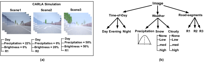
Figure 1. Scenes and feature representations: (a) scenes with feature labels from CARLA simulation, (b) hierarchical representation of an image using its features. The features can take discrete or continuous values.

State-of-the-art: Multi-chained one-class classifiers (Tsoumakas et al., 2009) are commonly used for solving the multi-label anomaly detection problem. But the performance of these chains deteriorates in the presence of strong label correlation  (Yeh et al., 2017). Additionally, training one classifier for each label gets expensive for real-world datasets which have a large label set  (Read et al., 2011). Another problem with traditional classifiers like Principal Component Analysis  (Ringberg et al., 2007), Support Vector Machine  (Schölkopf et al., 2001), and Support Vector Data Description (SVDD)  (Wang et al., 2013) is that they fail in images due to computational scalability  (Ruff et al., 2018).

To improve the effectiveness of the classifiers, researchers have started investigating probabilistic classifiers like gan  (Goodfellow et al., 2014) and vae  (Kingma and Welling, 2013). gan has emerged as the leading paradigm in performing unsupervised and semi-supervised ood detection  (Akcay et al., 2019; Zenati et al., 2018), but problems of training instability and mode collapse  (Creswell et al., 2018; Vu et al., 2019) have resulted in vae based methods being used instead. In particular, the vae based reconstruction approach has become popular for detecting ood data  (An and Cho, 2015; Cai and Koutsoukos, 2020). However, this approach is less robust in detecting anomalous data that lie on the boundary of the training distribution  (Denouden et al., 2018). To address this, the latent space generated by a vae is being explored  (Denouden et al., 2018; Vasilev et al., 2020; Sundar et al., 2020). The latent space is a collection of latent variables ($L$), where each latent variable is a tuple defined by the parameters ($\mu$,$\sigma$) of a latent distribution ($z$) and a sample generated from the distribution. However, the traditional approach of just training a single vae on all input data leads to unstructured and entangled distributions  (Klys et al., 2018), which makes the task of isolating the feature(s) responsible for ood hard.

This paper: Our approach in this work is to investigate use of latent space disentanglement for detecting ood images used by perception dnns. This idea builds upon recent progress in structuring and disentangling the latent space  (Bengio et al., 2013; Higgins et al., 2016). Effectively, the latent space generated by the encoder of a vae is a Gaussian mixture model of several overlapping and entangled latent variables, each of which encodes information about the image features. However, as can be seen in Fig. 2-a, the latent variables form a single large cluster which makes it hard to use them for ood detection. Disentanglement is a state of the latent space where each latent variable is sensitive to changes in only one feature while being invariant to changes in the others  (Bengio et al., 2013). That is, the single large cluster of Fig. 2-a is separated into several smaller clusters of single latent variables if the features are independent. Such disentangled latent variables have been successfully used in several tasks like face recognition  (Tran et al., 2017; Peng et al., 2017), video predictions  (Hsieh et al., 2018), and anomaly detection  (Wang et al., 2020). However, disentangling all the latent variables is extremely hard for real-world datasets and is shown to be highly dependent on inductive biases  (Locatello et al., 2019) and feature correlations.

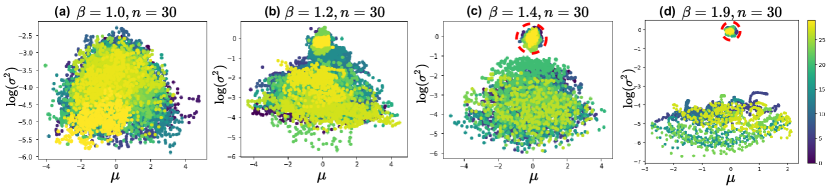
Figure 2. Visualizing Latent Space Disentanglement: Scatter plots illustrating the latent distributions ($\mu$, log($\sigma^{2}$)) generated using a $\beta$-VAE with different $\beta$ values. Each latent distribution in the latent space is represented using distinct color shades. CARLA images generated in Section 5 was used to generate these latent distributions. For $\beta$=1, the generated latent distributions are entangled. For $\beta>1$, the latent distributions are partially disentangled with a few latent distributions (inside the red circle) encoding independent features moving close to $\mu$=0 and log($\sigma^{2}$)=0, and the others moving away. Plot axis: x-axis represents the mean of the latent distributions in the range [-5,5], and the y-axis represents the log of variance in the range [-5,5].

Nevertheless, even partially disentangling the latent variables can lead to substantial gains as shown by Jakab et al. (Jakab et al., 2020) and Mathieu et al. (Mathieu et al., 2019). Partial disentanglement is a heuristic that groups the most informative latent variables into one cluster and the remaining latent variables that are less informative into another, as shown in Fig. 2-c. This selective grouping enables better separation in the latent space for the train and test images as shown in Fig. 10 (see Section 5). However, the procedure for training a disentangled latent space for real-world cps is hard. As a result, it is one of the aspects we focus on in this paper, along with interpreting the source of the ood.

Our Contributions: We present an approach to generate a partially disentangled latent space and learn an approximate mapping between the latent variables and the image features to perform ood detection and reasoning. The steps in our approach are data partitioning, latent space encoding, latent variable mapping, and runtime anomaly detection. To generate the partially disentangled latent space, we use a bvae, which has a gating parameter $\beta$ that can be tuned to control information flow between the features and the latent space. For a specific combination of $\beta$ $>1$ and the number of latent variables ($n$), the latent space gets partially disentangled with few latent variables encoding most of the feature’s information, while the others, encoding little information. We present a bo heuristic to find the appropriate combination of the $\beta$ and $n$ hyperparameters. The heuristic establishes disentanglement as a problem of tuning the two hyperparameters. The selected hyperparameters are used to train a bvae that is used by a latent variable mapping heuristic to select a set of most informative latent variables that are used for detection and identify the sensitivity of the latent variables towards specific features. The sensitivity information is used for reasoning the ood images. Finally, the trained bvae along with the selected latent variables are used at runtime for ood detection and reasoning. We demonstrate our approach on two cps case studies: (a) an av in CARLA simulator  (Dosovitskiy et al., 2017), and (b) a real-world automotive dataset called nuImages (nuscenes, [n.d.]).

Outline: The outline of this paper is as follows. We formulate the ood detection problem in Section 2. We introduce the background concepts in Section 3. We present our ood detection approach in Section 4. We discuss our experiment setup and evaluation results in Section 5. Finally, we present related research in Section 6 followed by conclusions in Section 7.

2. Problem Formulation

To set up the problem, consider a cps that uses a perception dnn trained on image distribution $\mathcal{T}$, where $\mathcal{T}$ = {$s_{1},s_{2},\dots,s_{i}$} is a collection of scenes. A scene is a collection of sequential images {$I_{1},I_{2},\dots,I_{m}$} generated from a training distribution $P(\mathcal{T})$. Every image in a scene is associated with a set of discrete or continuous valued labels ($I\rightarrow 2^{\mathbb{L}}$) belonging to the generative features of the environment (see Fig. 1). It is important to note that the sampling rate of images depends on the dynamics of the system. With this model, we can define the problems we study as follows:

Problem 1.

Given a test image $I_{t}$, determine (a) if $I_{t}\in P(\mathcal{T})$, and (b) if ($I_{t}\not\in P(\mathcal{T})$) then identify the feature $f$ whose $Label(I_{t},f)\not\in P_{f}(\mathcal{T})$, where $P_{f}$ is the training distribution on the feature $f$.

Example 0.

To illustrate the problem, we trained an NVIDIA DAVE-II dnn  (Bojarski et al., 2016) to perform e2e driving of an av in CARLA simulation. We trained the network on camera images from scene1 and scene2 (see Fig. 1) to predict the steering control action for the av. As shown in Fig. 3-a, the network’s steering predictions were accurate when tested on images from training scenes. However, the predictions got erroneous when we used the network to predict on images of a new scene (scene3) with higher precipitation values outside the training distribution (Fig. 3-b). The error in steering predictions caused the av crash of a sidewall. For this reason, if we knew that the precipitation level is compromising the network’s predictions, we can switch to an alternative controller that operates on other sensor inputs (e.g., Radar or Lidar) rather than the camera images.

Figure 3. Problem illustration: We trained an NVIDIA DAVE-II dnn with images from scene1 and scene2 (Fig. 1) to predict the steering values of an av that travels on a straight road segment in CARLA simulator. We tested the network on three test scenes: (a) A scene that had precipitation and brightness values within the training distribution, (b) A scene with high precipitation (60%) that was not in the training distribution. For this scene, the dnn predictions deviate from the nominal value shown in the plot a, and (c) A scene where brightness value changed from low (20%) to high (50%) at $t=10$ seconds. The dnn predictions were accurate until $t=10$ seconds, thereafter the predictions got erroneous.

Problem 2.

Given the test image $I_{t}$ at time $t$, the goal is to determine if $I_{t}$ has changed with respect to the previous images in a time series window $(I[t-M+1],\dots,I[t])$, where $M$ is the window size.

Example 0.

To illustrate the problem, we use the same av setup discussed in problem1. We tested the trained network on a new scene (scene4) with low brightness (in-distribution) for up to ten seconds, and the brightness was briefly high (ood) for the next ten seconds. For this scene, the network predicted accurately for the first ten seconds and erroneously for the next ten seconds as shown in Fig. 3-c. Such an abrupt change in the image feature increases the av’s risk of collision as demonstrated in our recent work (Hartsell et al., 2021). So, identifying the change points can be beneficial for reducing the system’s risk of a consequence.

Detector Requirements: We evaluate ood detectors that solve these problems against the following properties.

• Robustness - The detector should have low false positives and false negatives. A well known metric to measure robustness is F1-score = $(2\cdot Precision\cdot Recall)\div(Precision+Recall)$. Precision is computed as $TP\div(TP+FN)$, and Recall is computed as $TP\div(TP+FP)$. Where TP is True positive, FP is False positive, and FN is false negative.

• Minimum Sensitivity (MS) - The detector should have a minimum sensitivity towards each feature  (Martinez-Estudillo et al., 2008). For an image $I_{t}$ with feature labels $\mathbb{L}$={$l_{1},l_{2},\cdots l_{k}$}, minimum sensitivity is defined as the minimum value of the detector’s sensitivity for each feature label. $MS=min\{Si;i=1,2,\cdots,k\}$, where $S_{i}$ is the sensitivity of the detector to the feature $i$. Recall has been a well known metric to measure the detector’s sensitivity.

• Low Computation Overhead - Our target platforms are resource constrained autonomous cps like DeepNNCar (Ramakrishna et al., 2020). Therefore, the detector should have a low resource signature.

• Low Execution time - Autonomous cps typically have a small sampling period (typically 50 to 100 milliseconds). Therefore, the detector should have a low execution time that is smaller than the system’s sampling period.

3. Background

In this section, we provide an overview of several basic concepts that are required to understand our ood detection approach.

3.1. Kullback-Leibler (KL) divergence

kl  (Edwards, 2008) is a non-symmetric metric that can be used to measure the similarity between two distributions. For any probability distribution $p$ and $q$ the kl can be computed as illustrated in Eq. 1. A kl value close to zero indicates the two distributions are similar, while a larger value indicates their dissimilarity.

(1) $$\small D_{KL}(p||q)=\sum_{x\in\chi}p(x)log\frac{p(x)}{q(x)}$$

Recently, the kl metric is being utilized in several ways: (a) training loss function of different generative models (e.g., vae) called the elbo (Kingma and Welling, 2019), and (b) ood detection metric (Vasilev et al., 2020) that measures if the latent distributions generated by a generative model deviate from a standard normal distribution. The metric can be computed as shown below.

(2) $$\small KL(x)=D_{KL}(q_{\phi}(z_{i}|x)||\mathcal{N}(0,1))$$

Where, $\mathcal{N}(0,1)$ is a standard normal distribution. $q_{\phi}(z_{i}|x)$ is the distribution generated by the encoder of a vae for a latent variable $L_{i}$, and input $x$.

3.2. bvae ($\beta$-VAE)

bvae (Higgins et al., 2016) is a variant of the original vae with a $\beta$ hyperparameter attached to the kl (second term) of the elbo loss function shown in Eq. 3. The network has an encoder that maps the input data ($x$) distribution $P(x)$ to a latent space ($z$) by learning a posterior distribution $q_{\phi}(z|x)$. The decoder then reconstructs a copy of the input data ($x^{\prime}$) by sampling the learned distributions of the latent space. In doing so, the decoder also learns a likelihood distribution $p_{\theta}(x|z)$. The latent space is a collection of $n$ latent variables that needs to be selectively tuned in accordance with the input dataset. To remind, a latent variable is a tuple defined by the parameters ($\mu$,$\sigma$) of a latent distribution ($z$) and a sample generated from the distribution.

(3) $$ELBO(\theta,\phi,\beta;x,z)={\mathbb{E}}_{q_{\phi}(z|x)}[logp_{\theta}(x|z)]-\beta D_{KL}(q_{\phi}(z|x)||p(z))$$

$\theta$ and $\phi$ parameterize the latent variables of the encoder and the decoder, and $D_{KL}$ is the kl metric discussed in Section 3.1. The first term computes the similarity between the input data $x$ and the reconstructed data $x^{\prime}$. The second term computes the kl between $q_{\phi}(z|x)$ and a predefined distribution $p_{\theta}(x|z)$, which is mostly the standard normal distribution $\mathcal{N}(0,1)$.

Tuning $\beta$ for disentanglement: As suggested by Higgins et al.  (Higgins et al., 2016), $\beta$ controls the amount of information that flows from the features to the latent space, and an appropriate hyperparameter combination of $\beta$ $>1$ and $n$ is shown to disentangle the latent space for independent features. Fig. 2 shows the latent space disentanglement for different values of $\beta$ while $n$ is fixed to $30$. For $\beta$ $=1$, the latent distributions are entangled. With $\beta$ $>1$, the latent space starts to partially disentangle with a few latent variables (inside the red circle) encoding most information about the features stay as a cluster close to $\mu$=0 and log($\sigma^{2}$)=0, and the others are uninformative and form a cluster that lies farther. However, as the $\beta$ value gets larger ($\beta$=1.9), the information flow gets so stringent that the latent space becomes uninformative  (Mathieu et al., 2019). So, finding an appropriate combination of $\beta$ and $n$ for disentanglement is a hard problem. To address this problem, we provide a heuristic in Section 4.2.

3.3. mig

mig is a metric proposed by Chen, Ricky TQ et al.  (Chen et al., 2018) to measure the latent space disentanglement. It is an information theoretic metric that measures the mutual information between features and the latent variables. It measures the average difference between the empirical mutual information of the two most informative latent variables for each feature and normalizes this result by the entropy of the feature. mig is computed using the following equation.

(4) $$\footnotesize MIG=\frac{1}{|\mathcal{F}|}\sum_{f\in\mathcal{F}}\frac{1}{H(f)}(I_{1}(L_{j};f)-I_{2}(L_{j}^{\prime};f))$$

$I_{1}(L_{j};f)$ represents the empirical mutual information between the most informative latent variable $L_{j}$ and the feature $f$. $I_{2}(L_{j}^{\prime};f)$ represents the empirical mutual information between the second most informative latent variable $L_{j}^{\prime}$ and the feature $f$. $H(f)$ is the entropy of information contained towards the feature $f$. In this work, we use mig as a measure for selecting the right hyperparameter combination ($\beta$ and $n$) for the bvae.

Algorithm 1 Computing MIG

Parameter: number of latent variables $n$, image features $\mathcal{F}$, number of iterations $t$, trained bvae

Input: data partition $\mathcal{P}=\{P_{1},P_{2},....,P_{m}\}$

Output: average MIG

1:while $i\leq t$ do

2:    Generate latent variable parameters ($\mu$, $\sigma$) using a trained bvae

3:    for each $P\in\mathcal{P}$ do

4:        Extract $\mu$, $\sigma$ parameters

5:        Compute feature entropy H(f)

6:        Compute latent variable entropies $H(L_{j})$ and $H(L_{j}^{\prime})$

7:        Compute conditional entropies $H(L_{j}|f)$ and $H(L_{j}^{\prime}|f)$

8:        Compute Mutual Information of most informative latent variable $I_{1}(L_{j};f)=H(L_{j})-H(L_{j}|f)$

9:        Compute Mutual Information of second most informative latent variable $I_{2}(L_{j}^{\prime};f)=H(L_{j}^{\prime})-H(L_{j}^{\prime}|f)$

10:    end for

11:    compute $MIG=\frac{1}{|\mathcal{P}|}\sum_{f\in\mathcal{P}}\frac{1}{H(f)}(I_{1}(L_{j};f)-I_{2}(L_{j}^{\prime};f))$

12:    Append MIG to $L$

13:end while

14:return average MIG = sum($L$)/$t$

Implementation: We have implemented Algorithm 1 to compute mig. Since mig is computed based on entropy, the training set $\mathcal{T}$ should have images with feature labels that take different discrete and continuous values as shown in Fig. 1. For the ease of computation, we partition $\mathcal{T}$ into different partitions $\mathcal{P}$ using our approach discussed in Section 4.1. Our approach is to create partitions such that each partition will have images that have a variance in the value of a specific feature $f$, irrespective of the variance in the others. The feature with the highest variance represents the partition. Then, in each iteration, we use the feature representing the partition to compute the feature entropy, the conditional entropy, and the mutual information of the two most informative latent variables. The mutual information is then used to compute the mig as shown in the algorithm. Finally, for robustness, we average the mig across $t$ iterations.

Complexity Analysis: The complexity of the mig algorithm in worst case is $O(t*|\mathcal{P}|*nq*|\mathcal{F}|*|\mathcal{T}|*n^{2}*ns)$. Where $t$ is the number of iterations, —$\mathcal{P}$— is the number of partitions, $n$ is the number of latent variables, —$\mathcal{F}$— is the number of features considered for the calculations, $nq$ is the number of unique values that each feature has in the partition (e.g., for a partition with brightness=10%, and brightness=20%, $nq$=2), $ns$ is the number of samples generated from each latent variable, and $|\mathcal{T}|$ is the size of training data. The specific values of these parameters for the av example in CARLA simulation are $t=5$, $|p|=2$, $n=30$, $\mathcal{F}=2$, $ns=500$, and $nq$=3.

3.4. icp (ICP)

icp is a variant of the Conformal Prediction algorithm  (Vovk et al., 2005) that tests if a test observation ($x_{t}$) conforms to every observation in the training dataset ($\mathcal{T}$). However, comparing $x_{t}$ to every observation of $\mathcal{T}$ is expensive and gets complex with the size of $\mathcal{T}$. To address this, icp splits $\mathcal{T}$ into two non-overlapping sets called as the proper training set ($\mathcal{T}_{P}$) which is used to train the prediction algorithm (e.g., dnn) and the calibration set ($\mathcal{C}$) which is used to calibrate the test observations. In splitting the datasets, icp performs a comparison of the $x_{t}$ to each element in the $\mathcal{C}$ which is a smaller representative set of $\mathcal{T}$. The icp algorithm has two steps: The first step involves, computing the non-conformity measure, which represents the dissimilarity between $x_{t}$ to the elements in the set $\mathcal{C}$. The non-conformity measure is usually computed using conventional metrics like euclidean distance or K-nearest neighbors. But, in this work we use kl as the non-conformity measure. The next step involves computing the p-value, which serves as evidence for the hypothesis that $x_{t}$ conforms to $\mathcal{C}$. Mathematically, the p-value is computed as the fraction of the observations in $\mathcal{C}$ that have non-conformity measure above the test observation $x_{t}$: $p_{x_{t}}=|\{\forall\alpha\in\mathcal{C}|\alpha\geq\alpha_{x_{t}}\}|/|\mathcal{C}|$. Note for brevity, we drop the notation of $x$ and just use the term $p_{t}$ and $\alpha_{t}$. Here $\alpha$ denotes the non-conformity measure for each observation in $\mathcal{C}$ and $\alpha_{t}$ denotes the non-conformity measure for $x_{t}$.

Once $p_{t}$ is computed, it can be compared against a threshold $\tau$ $\in$ (0,1) to confirm if $x_{t}$ belongs to $\mathcal{T}$. However, such a threshold-based comparison is only valid if each test observation is i.i.d (independent and identically distributed) to $\mathcal{T}$, which is not true for cps  (Cai and Koutsoukos, 2020). Although the assumptions about i.i.d are not valid, icp can still be applied under the weaker assumption of exchangeability. In our context, exchangeability means to test if the observations in $\mathcal{C}$ have the same joint probability distribution as the sequence of the test observations under consideration (are they permutations of each other). If they are, then we can expect the p-values to be independent and uniformly distributed in [0, 1] (Theorem 8.2,  (Vovk et al., 2005)), which can be tested using the martingale. Exchangeability martingale (Fedorova et al., 2012) has been used as a popular tool for testing the exchangeability and the i.i.d assumptions of the test observation with respect to $\mathcal{C}$. So, once the p-value for a test observation is computed, the simple mixture martingale (Fedorova et al., 2012) can be computed as $\mathcal{M}_{t}=\int_{0}^{1}\left[\prod_{i=1}^{t}\epsilon p_{i}^{\epsilon-1}\right]d\epsilon$.

Also, it is desirable to use a sequence of test observations rather than a single observation for improving the detection robustness. However, the observations received by cps are in time series, which makes them non-exchangeable (Cai and Koutsoukos, 2020). The non-exchangeability nature hinders the direct application of the martingale to an infinitely long sequence of test observations. To address this, the authors in (Cai and Koutsoukos, 2020) have suggested applying the martingale over a short window of the time series in which the test observations can be assumed to be exchangeable. Then, the simple mixture martingale over a short time window $[t-M+1,t]$ of past $M$ p-values can be computed as $\mathcal{M}_{t}=\int_{0}^{1}\left[\prod_{i=t-M+1}^{t}\epsilon p_{i}^{\epsilon-1}\right]d\epsilon$. The martingale will grow over time if and only if there are consistently low p-values within the time window, and the corresponding test observations are i.i.d. Otherwise, the martingale will not grow. It is important to note that the martingale computation is only valid for a short time window. The size of the window is dependent on the cps dynamics, like the speed of the system. In our experiments, the system’s speed was constant, so we used a fixed window size of $20$ images.

3.5. cusum

One of the problems we are dealing with is change detection. This problem is traditionally solved using cusum  (Basseville et al., 1993), which is a statistical quality control procedure used to identify variation based on historical data. It is computed as $S_{0}$ = 0 and $S_{t+1}$ = max(0, $S_{t}$+$x_{t}$-$\omega$), where $x_{t}$ is the sample from a process, $\omega$ is the weight assigned to prevent $S_{t}$ from consistently increasing to a large value. $S_{t}$ can be compared to a predefined threshold $\tau$ to perform the detection. $\omega$ and $\tau$ are hyperparameters that decide the detector’s precision.

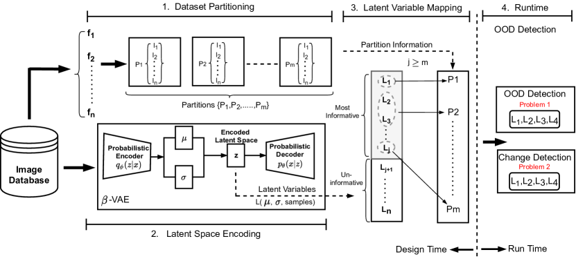
Figure 4. Detector design approach. The steps of our approach include data partitioning, latent space encoding, latent variable mapping and runtime ood detection.

4. Our Approach

In this section, we present our approach that uses a bvae to perform latent space based ood detection and reasoning. Our approach is shown in Fig. 4 and the steps involved work as follows: First, we divide the multi-labeled datasets into partitions based on the variance in the feature values. A partition consists of images with one feature having higher variance in its values compared to others. Second, we generate a partially disentangled latent space using a bvae. As discussed earlier, the combination of $\beta$ and $n$ influence the level of latent space interpretability. To find the optimal combination, we propose a heuristic that uses the bo algorithm  (Snoek et al., 2012) along with mig to measure disentanglement. Third, we discuss a heuristic to perform latent variable mapping to identify the set of latent variables $\mathcal{L}_{d}$ that encodes most information of the image features. These latent variables are collectively used as the detector for ood detection. Further, we perform a kl based sensitivity analysis to identify the latent variable(s) $\mathcal{L}_{f}$ $\subseteq$ $\mathcal{L}_{d}$, that is sensitive to specific features. The latent variable(s) in $\mathcal{L}_{f}$ are used as reasoners to identify the ood causing features. We discuss these steps in the rest of this section.

4.1. Data partitioning

Data partitioning is one of the core steps of our approach. It is required for implementing the mig and the latent variable mapping heuristics. We define a partition $P$ as a collection of images that have higher variance in the value of one feature as compared to the variances in the values of other features. To explain the concept of a partition, consider the features of images in training set $\mathcal{T}$ to be $\mathcal{F}=\{f_{1},f_{2},...,f_{n}\}$, and each feature can take a value either discrete or continuous as shown in Fig. 1. We normalize these values for the ease of partitioning. Our goal is to group images in $\mathcal{T}$ into $m$ partitions $\mathcal{P}$ = $\{P_{1},P_{2},....,P_{m}\}$, such that a partition $P_{j}$ will have all the images with high variance in the values of feature $f_{j}$. For creating these partitions, we generate sub-clusters for each discrete valued feature(s) and sub-clusters for each continuous valued feature. In each of these sub-clusters, only the value of the feature under consideration $f_{j}$ changes while the value of other features remains unchanged. The clustering is done effectively through an agglomerative clustering algorithm. Thereafter, the partition for a feature is the union of all sub-clusters which can be represented as $P_{j}$ = $\{C_{1}\cup C_{2}....\cup C_{n}\}$. It is important to note that each partition should have $variance>0$ in the value of the feature under consideration ($f_{j}$), irrespective of changes in the values of other features. To illustrate the partitioning concept, consider the example scenes in Fig. 1. A precipitation partition for this example is a collection of images from two combinations, $C1$ = {day, precipitation=22%, brightness=0%, R1}, and $C2$ = {day, precipitation=50%, brightness=50%, R1}.

Our data partitioning approach works well for datasets with well defined labels that provide feature value(s). However, real-world automotive datasets such as nuScenes  (Caesar et al., 2020) and nuImages  (nuscenes, [n.d.]) provide semantic labels that are not always well defined, and they do not contain feature values. Also, they often have images in which several feature values change at once. Since the feature related information is not fully available, some prepossessing and thresholds selection for feature values are required for partitioning. Currently, the threshold selection for partitioning is performed by a human supervisor, but we want to automate it in the future. We have applied this partitioning technique on the nuScenes dataset in our previous work (Sundar et al., 2020) and used it in this work for partitioning the nuImages dataset.

4.2. Latent Space Encoding

The second step of our design procedure is the selection and training of bvae to generate a partially disentangled latent space encoding. However, the challenge is to determine the best combination of the $\beta$ and $n$ hyperparameters. To find this, we propose a novel greedy heuristic that formulates disentanglement as a hyperparameter search problem. The heuristic uses bo (BO) algorithm with mig as the objective function to maximize.

Implementation: The bo algorithm builds a probability model of the objective function and uses it to identify the optimal model hyperparameter(s). The algorithm has two steps: a probabilistic Gaussian Process model that is fitted across all the hyperparameter points that are explored so far, and an acquisition function to determine which hyperparameter point to evaluate next (Snoek et al., 2012). We use these steps to search for an optimal hyperparameter for n $\in$ $N$, and $\beta$ $\in$ $B$. The heuristic using bo algorithm is shown in Algorithm 2, and the steps are discussed below.

Algorithm 2 Bayesian Optimization Hyperparameter Selection

Parameter: number of iterations $t$, initialization iterations $k$, explored list $\mathcal{X}$

Input: training set $\mathcal{T}$, data partition $\mathcal{P}$, $N$, $B$

Output: best $n$ and $\beta$

1:for $x=1,2,...,t$ do

2:    if $x\leq k$ then

3:        Randomly sample $n$, $\beta$ from $N$ and $B$

4:    else

5:        Find $n$, $\beta$ that optimizes the acquisition function over Gaussian Process

6:    end if

7:    Train bvae on $\mathcal{T}$ using the selected $n$ and $\beta$

8:    Compute Average MIG

9:    Append $n$, $\beta$ and MIG to $\mathcal{X}$

10:    Update the Gaussian Process posterior distribution using $\mathcal{X}$

11:end for

12:return $n$ and $\beta$

First, for $k$ initial iterations, we randomly pick values for $\beta$ and $n$ from the hyperparameter search space. The randomly selected n and $\beta$ combination is used to train a bvae network and compute the mig as discussed in Algorithm 1. The selected hyperparameters and the computed mig are added to an explored list $\mathcal{X}$. After the initial iterations, the trained Gaussian Process model (the initial iterations are used to train and stabilizes the Gaussian process model) is fitted across all the hyperparameter points that were previously explored, and the marginalization property of the Gaussian distribution allows the calculation of a new posterior distribution g($x_{n}$) with posterior belief $\tilde{g}(x_{n})$. Finally, the parameters ($\mu$, $\sigma$) of the resulting distribution are determined to be used by the acquisition function, which uses the posterior distribution to evaluate new candidate hyperparameter points.

Second, an acquisition function is used to guide the search by selecting the hyperparameter(s) for next iteration. For this, it uses the $\mu$ and $\sigma$ computed by the Gaussian process. A commonly used function is the expected improvement (EI)  (Jones et al., 1998; Gardner et al., 2014), which can described as follows. Consider, $x_{n}$ to be some hyperparameter(s) point in the distribution g($x_{n}$) with posterior belief $\tilde{g}(x_{n})$, and $x_{+}$ is the best hyperparameter(s) in $\mathcal{X}$ (explored list), then the improvement of the point $x_{n}$ is computed against $x_{+}$ as $I(x_{n})=max\{0,(g(x_{+})-g(x_{n}))\}$. Then, the expected improvement is computed as $EI(x_{n})=\mathbb{E}\big{[}I(x_{n})|x_{n}\big{]}$. Finally, the new hyperparameter(s) is computed as the point with the largest expected improvement as $x_{n+1}=argmax(EI(x_{n}))$. The new hyperparameter point is used to train a bvae and compute the MIG, which is then added to the explored list $\mathcal{X}$. The list $\mathcal{X}$ is used to update the posterior distribution of the Gaussian process model in the next iteration. The two steps of the algorithm are iterated until maximum number of iterations is reached or can be terminated early if optimal hyperparameter(s) is consecutively selected by the algorithm for $j$ iterations (we chose $j$=3 in this work).

Design Space Complexity: Searching for optimal hyperparameters is a combinatorial problem that requires optimizing an objective function over a combination of hyperparameters. In our context, the bvae hyperparameters to be selected are $\beta$ and $n$, and the objective function to optimize is the mig whose complexity we have reported in the previous section. The range of the hyperparameters are n $\in$ $\{n_{1},n_{2},\dots,n_{l}\}$ and $\beta$ $\in$ $\{\beta_{1},\beta_{2},\dots,\beta_{m}\}$. The hyperparameter search space then becomes the Cartesian product of the two sets. In the case of the grid search, each point of this search space is explored, which requires training the bvae and computing mig. Grid search suffers from the curse of dimensionality since the number of evaluations exponentially grows with the size of the search space  (Hutter et al., 2019). In comparison, the random search and bo algorithms do not search the entire space but search for a selected number of iterations $t$. While random search selects each point in the search space randomly, the bo algorithm performs a guided search using a Gaussian process model and the acquisition function.

In bo algorithm, the first $k$ iterations stabilize the Gaussian Process model using randomly selected points in the space to train a bvae and compute the mig. After these iterations, the Gaussian process model is fitted to all the previously sampled hyperparameters. Then, the acquisition function based on expected improvement uses the posterior distribution of the Gaussian process model to find new hyperparameter(s) that may optimize the mig. The new hyperparameter(s) are used to train a bvae and compute the MIG. So, this process is repeated for $t$ iterations, and in every iteration, a bvae is trained, and the mig is computed as shown in Algorithm 2. This intelligent search mechanism based on prior information makes the search technique efficient as it takes a smaller number of points to explore in the search space as compared to both grid search and random search  (Snoek et al., 2012; Hutter et al., 2019). The bo algorithm has a polynomial time complexity because the most time consuming operation is the Gaussian process which takes polynomial time  (Hutter et al., 2019). We report the experimental results for the three hyperparameter algorithms in Table 1. As seen in the Table, the bo algorithm takes the least time and iterations to select the hyperparameters that achieve the best mig value as compared to the other algorithms.

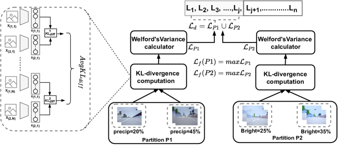
Figure 5. Latent Variable Mapping: Heuristic based on kl and Welford’s variance calculator to select latent variables for $\mathcal{L}_{d}$ and $\mathcal{L}_{f}$.

4.3. Latent Variable Mapping

Given the data partition set $\mathcal{P}$ and a trained bvae that can generate the latent variable set $\mathcal{L}$, we find the most informative latent variables set $\mathcal{L}_{d}$ $\subseteq$ $\mathcal{L}$ that encodes information about the image features in the training set $\mathcal{T}$. As discussed earlier, the most informative latent variables form a separate cluster from the less informative ones when we partially disentangle the latent space using the bo heuristic. Although the most informative latent variables are separately clustered in the latent space, we need a mechanism to identify them. To do this, we present a kl based heuristic that is illustrated in Fig. 5.

The latent variables in $\mathcal{L}_{d}$ are used as detectors i.e., they can detect overall distribution shifts in the images (we discuss the exact procedure later). However, this does not solve the problem of identifying the specific feature(s) whose labels caused the ood. For this, given the representative feature $f$ of a partition has high variance, we identify the subset of latent variable(s) $\mathcal{L}_{f}\subseteq\mathcal{L}_{d}$ that is sensitive to the variations in $f$. For example, if we have a partition with images that have different values in the precipitation (e.g., precipitation=20%, precipitation=50%, etc.), then we map latent variable(s) that are sensitive to changes in precipitation level. The latent variable(s) in $\mathcal{L}_{f}$ is called the reasoner for feature $f$ and is used to identify if $f$ is responsible for the ood. The steps in our heuristic are listed in Algorithm 3 and it works as follows: For each partition, $P\in\mathcal{P}$, and for each scene $s\in P$, we perform the following steps.

Algorithm 3 Selecting Latent Variables for $\mathcal{L}_{d}$ and $\mathcal{L}_{f}$

Parameter: global list $G$

Input: data partitions $\mathcal{P}$ = $\{P_{1},P_{2},...,P_{m}\}$, number of latent variables $n$

Output: $\mathcal{L}_{d}$ and $\mathcal{L}_{f}$ for each partition

1:for each $P\in\mathcal{P}$ do

2:    for each $s\in P$ do

3:        for $l=1;\ l<=len(s);\ l=l+1$ do

4:           for $i=0,1,2,.....,n$ do

5:               $KL^{i}(x_{l})=D_{KL}(q_{\phi}(z_{i}|x_{l})||\mathcal{N}(0,1))$

6:               $KL^{i}(x_{l+1})=D_{KL}(q_{\phi}(z_{i}|x_{l+1})||\mathcal{N}(0,1))$

7:               $KL^{i}_{l}(diff)=|KL^{i}(x_{l+1})-KL^{i}(x_{l})|$

8:           end for

9:        end for

10:        for $i=1,2,....,n$ do

11:           $AvgKL_{diff}^{i}=\frac{1}{len(s)-1}\sum_{l=1}^{len(s)-1}KL^{i}_{l}(diff)$

12:        end for

13:        Store $AvgKL_{diff}^{i}$ to $G$

14:    end for

15:    Use Welford’s algorithm to select $\mathcal{L}_{P}$, which is a set of $m$ latent variables with high variance in $AvgKL^{i}_{diff}$

16:    $\mathcal{L}_{f}$ = max($\mathcal{L}_{P}$)

17:end for

18:$\mathcal{L}_{d}$ = $\{\mathcal{L}_{P_{1}}\cup\mathcal{L}_{P_{2}}\cup.....\cup\mathcal{L}_{P_{m}}\}$

19:return $\mathcal{L}_{d}$, $\{\mathcal{L}_{f_{1}},\mathcal{L}_{f_{2}},...,\mathcal{L}_{f_{m}}\}$

First, we take two subsequent images $x_{l}$ and $x_{l+1}$ and pass each of them separately to the trained bvae to generate the latent variable set $\mathcal{L}$ for each of the images. As a remainder, $\mathcal{L}$ is a collection of $n$ latent variables, and each latent variable has a latent distribution ($z$) with parameters $\mu$ and $\sigma$. Then, for each latent variable of the images ($x$) we compute a kl between its latent distribution $q(z_{i}|x)$ and the standard normal distribution $\mathcal{N}(0,1)$ as discussed in Section 3.1. The computed kl is $KL^{i}(x)=D_{KL}(q(z_{i}|x)||\mathcal{N}(0,1))$.

Second, we calculate the kl difference between corresponding latent variables of the two images as: $KL^{i}_{l}(diff)=|KL^{i}(x_{l+1})-KL^{i}(x_{l})|$. This procedure is repeated across all the subsequent images in the scene $s$.

Third, we compute an average kl difference for each latent variable across all the subsequent images of the scene as follows.

(5) $$\footnotesize AvgKL_{diff}^{i}=\frac{1}{len(s)-1}\sum_{l=1}^{len(s)-1}KL^{i}_{l}(diff)$$

where $KL^{i}_{l}(diff)$ is the kl difference of the latent variable $L_{i}$ for the $l^{th}$ subsequent image pair in a scene $s$ and $len(s)$ is the number of images in $s$. This value indicates the average variance in the kl value across each latent variable for all the images in the $s$. This approach of computing the variations across $s$ is motivated from the manual latent variable mapping technique in (Higgins et al., 2016). Further, the $AvgKL^{i}_{diff}$ value is computed $\forall s\in P$.

Fourth, we then use the Welford’s variance calculator  (Welford, 1962) to compute the variance in the $AvgKL^{i}_{diff}$ value across all the scenes in the partition. Welford’s variance calculator computes and updates the variance in a single pass as the measurements are available. It does not require storing the measurements till the end for the variance calculation, which will make the variance calculation across several scenes faster. In our case, the variance calculator returns a partition latent variable set $\mathcal{L}_{P}$, which is a set of top $m$ latent variables that has the highest $AvgKL^{i}_{diff}$ across all images in $P$. Selecting an appropriate number of latent variables ($m$) for $\mathcal{L}_{P}$ is crucial, as we use it to select the latent variables for $\mathcal{L}_{d}$ and $\mathcal{L}_{f}$. The value for $m$ is chosen empirically, and the selection depends on the variances across the scenes of a partition. However, it is important to note that selecting a small value for $m$ may not include all the informative latent variables required for detection and choosing a large value for $m$ may include uninformative latent variables that may reduce the detection accuracy and sensitivity.

Further, we choose the top latent variable(s) from $\mathcal{L}_{P}$ and use it as the reasoner ($\mathcal{L}_{f}$) for the partition. If the partition has variance in an independent image feature (e.g., brightness), then a single best latent variable which has the most sensitivity can be used as the reasoner. However, if the feature is not independent, then more than one latent variable needs to be used, and the size of $\mathcal{L}_{P}$ increases. Besides, if two features correlate, then a single latent variable may be sensitive to both features. If such a latent variable is used for reasoning at runtime, and if it shows variation, then we attribute both the features to be responsible for the ood.

Finally, these steps are repeated for all the partitions in $\mathcal{P}$, and the latent variables for $\mathcal{L}_{d}$ is formed by $\{\mathcal{L}_{P_{1}}\cup\mathcal{L}_{P_{2}}\cup\dots\cup\mathcal{L}_{P_{m}}\}$. If the latent space is partially disentangled, then the top $m$ latent variables in each $\mathcal{L}_{P}$ will mostly be the same. Otherwise, the number of similar latent variables in each $\mathcal{L}_{P}$ will be small.

4.4. Runtime ood Detection

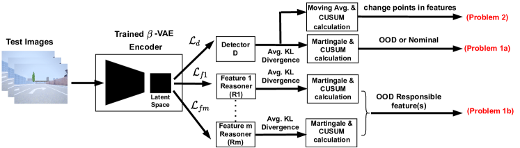
Figure 6. Runtime ood detection pipeline: The trained bvae detector at runtime provides three outputs that are sent to the decision manager to select an appropriate controller or control action that can mitigate the ood problems as discussed in Section 2.

At runtime, we use the trained bvae and the latent variable set $\mathcal{L}_{d}$ and $\mathcal{L}_{f}$ to detect ood problems discussed in Section 2. Fig. 6 shows the pipeline for runtime ood detection, and it works as follows. As a test image $x_{t}$ is observed, the encoder of the trained bvae is used to generate the latent space encoding. Then, the respective latent variables in ($\mathcal{L}_{d}$, $\mathcal{L}_{f}$) are sent to different processes to compute the average KL-divergence between the latent variables in $\mathcal{L}_{d}$ or latent variable(s) in $\mathcal{L}_{f}$ for the identified features. The kl is computed between each latent variables in $\mathcal{L}_{d}$ and $\mathcal{L}_{f}$, and the normal distribution $\mathcal{N}(0,1)$ as shown in Eq. 6.

(6) $$\alpha_{t}=KL(x_{t},\mathcal{N}(0,1))=\frac{1}{L}\sum_{l=1}^{L}|D_{KL}(q(z_{l}|x_{t})||\mathcal{N}(0,1))|$$

Where $L$ is the number of selected latent distributions; for the detector, it is the number of latent variables in $\mathcal{L}_{d}$, and for each feature, it is the number of latent variables in $\mathcal{L}_{f}$.

To detect the first ood problem (Problem 1), the kl is used as the non-conformity score to compute the icp and martingale score as shown in Algorithm 4. However, as the martingale can grow large very rapidly, we use the log of martingale. Then, a cusum over the log of martingale is computed to identify when the martingale goes consistently high. The cusum value $S_{t}$ of the detector latent variables $\mathcal{L}_{d}$ is compared against a detector threshold ($\tau_{d}$) to detect if the image $x_{t}$ is ood compared to the calibration set. Then, the cusum value $S_{t}$ of the reasoner latent variables $\mathcal{L}_{f}$ is compared against a reasoner threshold ($\tau_{r}$) to identify if the known feature(s) is responsible for the ood as discussed in Problem 1b of Section 2. The thresholds are empirically tuned as a tradeoff between false positives and mean detection delay (Basseville et al., 1993).

Algorithm 4 $\beta$-VAE based OOD detection using ICP

Parameter: sliding window length $M$, non-conformity measures of calibration set $\mathcal{C}$.

Input: image $x_{t}$ at time $t$, set of detector latent variables $\mathcal{L}_{d}$.

Output: martingale score $\log\mathcal{M}_{t}$ at time $t$

1:$\alpha_{t}=\sum_{\forall l\in\mathcal{L}_{d}}|D_{KL}(q(z_{l}|x_{t})||\mathcal{N}(0,1))|$

2:$p_{t}=\frac{\left(|\{\forall\alpha\in\mathcal{C}|\alpha\geq\alpha_{t}\}|\right)}{\left(|\mathcal{C}|\right)}$

3:$M_{t}=\int_{0}^{1}\left[\prod_{i=t-M+1}^{t}\epsilon p_{i}^{\epsilon-1}\right]d\epsilon$

4:return $\log\mathcal{M}_{t}$

To detect the second ood problem (Problem 2), the latent variables in $\mathcal{L}_{d}$ is used with sliding window moving average and cusum for change point detection. For this, the average kl of all the latent variables in $\mathcal{L}_{d}$ is computed using Eq. 6, and a moving average of the average kl ($A_{KL}$) is computed over a sliding window [$x_{t-M+1}$,…,$x_{t}$] of previous $M$ images in the time series. $A_{KL}$ is used to compute the cusum value $S_{t}$, which is compared against a threshold $\tau_{cp}$ to detect changes.

Finally, the outputs of the detector (See Fig. 6) are sent to the decision manager, which can use these detection results to perform system risk estimation (Hartsell et al., 2021) or high level controller selection using simplex strategies (Seto et al., 1998). In this work, we use a simple decision logic that uses the ood detection result to perform a control arbitration from the dnn controller to an autopilot controller.

5. Experiments and Results

We evaluate our approach using an av example in the CARLA simulator (Dosovitskiy et al., 2017) and show the preliminary results from the real-world nuImages dataset (nuscenes, [n.d.]). The experiments in this section were performed on a desktop with AMD Ryzen Threadripper 16-Core Processor, 4 NVIDIA Titan Xp GPU’s and 128 GiB memory.

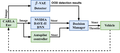
Figure 7. av block diagram: The components in green come inbuilt with the CARLA simulator, while the components in blue are designed for our example. While the simulator requires a GPU, the other components are run on one CPU core to emulate a resource constrained setting.

5.1. System Overview

Our first example system is an av which must navigate different road segments in town1 of the CARLA simulator. The architecture of our av, shown in Fig. 7, relies on a forward-looking camera for perception and a speedometer for measuring the system’s speed. It uses the NVIDIA DAVE-II dnn (Bojarski et al., 2016) as the primary controller and the simulator’s inbuilt autopilot mode as the secondary safety controller. In addition, a trained bvae detector and reasoner are used in parallel to the two controllers. The detection results and the steering values from the two controllers are sent to a simplex decision manager, which selects the appropriate steering value for the system based on the detection result. That is, if the detector returns the image to be ood, the decision manager selects the autopilot controller to drive the av. The sampling period used in the simulation is 1/13 seconds, and the vehicle moves at a constant speed of $0.5$ m/s for all our experiments.

5.1.1. Operating modes

Our av has two operating modes: (a) manual driving mode, which uses CARLA’s autopilot controller to drive around town1. The autopilot controller is not an AI component, but it uses hard-coded information from the simulator for safe navigation. We use this mode to collect the training set $\mathcal{T}$ and the test set ($\mathcal{T}_{t}$). These datasets are a collection of several CARLA scenes generated by a custom sdl shown in Fig. 8; and (b) autonomous mode, which uses a trained NVIDIA DAVE-II dnn controller to drive the av. In this setup, the bvae detector is used in parallel to the dnn controller to perform ood detection.

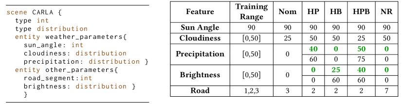
Figure 8. Data Generation: (left) A fragment of our sdl. (right) Scenes in CARLA simulation: Nominal scene ($Nom$) is generated by randomly sampling the features in their training ranges. High Precipitation ($HP$), High Brightness ($HB$), High Precipitation & Brightness ($HPB$) scene, and New Road ($NR$) are test scenes for which the feature values change from a training range value to a value outside the range at $t=20$ seconds. The initial values of precipitation and brightness are highlighted in green.

5.1.2. Data Generation

Domain-specific sdl such as Scenic  (Fremont et al., 2019) and MSDL  (foretellix, [n.d.]) are available for probabilistic scene generation. However, they did not fit our need to generate partition variations. Hence, we have implemented a simple sdl in the textX  (Dejanović et al., 2017) meta language (See Fig. 8), which is combined with a random sampler over the range of the simulator’s features like sun altitude, cloudiness, precipitation, brightness, and road segments to generate different scenes.

Train Scenes: The training feature labels, and their values are shown in Fig. 8. These features were randomly sampled in the ranges shown in Fig. 8 to generate eight scenes of $750$ images each that constituted the training set $\mathcal{T}$. Among these, two scenes had precipitation of 0%, the brightness of $0\%$, sun angle $90$°, cloudiness of $25\%$, and road segment of $1$ and $2$ for each scene, respectively. Three scenes had different precipitation values (precip=$5\%$, precip=$40\%$, precip=$50\%$) while sun angle took a value of $90$°, cloudiness took a value of $25\%$, brightness took a value of $0\%$, and $10\%$, and the road segments took a value of $1$ and $2$. The remaining three scenes had different brightness values (bright=$9\%$, bright=$25\%$, bright=$40\%$), precipitation took a value of $0\%$ and $5\%$, and all the other parameters remained the same as the other scenes. We split $6000$ images of $\mathcal{T}$ into $4000$ images of $\mathcal{T}_{P}$ and $2000$ images of $\mathcal{C}$ in the standard 2:1 ratio (page 222 of (Hastie et al., 2009)) for icp calculations.

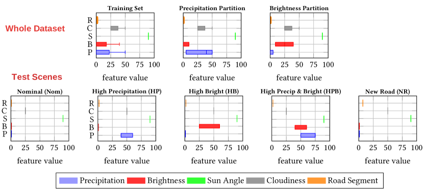
Figure 9. Feature Value Variance: Plots representing the normalized values of sun angle (S), cloudiness (C), precipitation (P), brightness (B), and road segments (R) for the training set, partitions, and the test scenes. We use the test scene abbreviations $Nom$ (Nominal), $HP$ (High Precipitation), $HB$ (High Brightness), $HPB$ (High Precipitation & Brightness), and $NR$ (New Road segment) for the rest of the paper. The $NR$ scene has all the feature values like the $Nom$ scene, but it uses the road segment $7$ that is not in the training distribution.

Test Scenes: The test scenes included a nominal scene ($Nom$) and four ood scenes as shown in Fig. 8. Each scene was $20$ seconds long, and it had $260$ images. (1) Nominal Scene ($Nom$) was an in-distribution scene generated from the training distribution. (2) High Precipitation ($HP$) scene was an ood scene in which the precipitation was increased from $40\%$ (in training range) to $60\%$ (out of training range) at $t=2$ seconds. (3) High Brightness ($HB$) scene was an ood scene in which the brightness was increased from $25\%$ (in training range) to $60\%$ (out of training range) at $t=2$ seconds. (4) High Precipitation & Brightness ($HPB$) scene was also an ood scene in which both the precipitation and the brightness were increased out of the training range at $t=2$ seconds. (5) New Road ($NR$) scene was an ood scene with a new road segment (segment=$7$) that was not in the training range, but the other features remained within the training range. Fig. 9 shows the variance in the normalized values of the scene features for the training set, partitions, and test scenes.

5.2. $\beta$-VAE Detector

We implement the steps of our approach discussed in Section 4 to design a bvae detector for our av example.

5.2.1. Data Partitioning

Using our partitioning technique discussed in Section 4.1, we select three scenes with variance in precipitation values (precip=$5\%$, precip=$40\%$, precip=$50\%$) as the precipitation partition $P1$, and the remaining three scenes with variance in brightness values (bright=$9\%$, bright=$25\%$, bright=$40\%$) as the brightness partition $P2$.

5.2.2. Latent Space Encoding

We applied the bo algorithm based heuristic discussed in Section 4.2 to select and train the bvae with appropriate hyperparameters.

Network Structure and Training: We designed a bvae network that has four convolutional layers $32/64/128/256$ with $5x5$ filters and $2x2$ max pooling followed by four fully connected layers with $2048$, $1000$, $250$ and $50$ neurons. A symmetric deconvolutional decoder structure is used as a decoder. This network along with images in $\mathcal{T}$ was used in the bo algorithm discussed in Algorithm 2. For each iteration of the bo algorithm, the network was trained for $100$ epochs using the Adam gradient-descent optimizer and a two-learning scheduler, that had an initial learning rate $\eta$ = $1$ x $10$^$-5$ for $75$ epochs, and subsequently fine-tuning $\eta$ = $1$ x $10$^$-6$ for $25$ epochs. Learning rate scheduler is used to improve the model’s accuracy and explore areas of lower loss. In addition, we had an early stopping mechanism to prevent the model from overfitting.

Algorithm	# of Iterations	Iterations to reach optimum	Search Time (min)	max MIG	Selected Parameter
Grid	360	5	10924.55	0.0017	30,1.4
Random	50	40	1199.51	0.00032	40,1.5
BO	50	16	837.05	0.0018	30,1.4

Table 1. Comparing Hyperparameter search algorithms: bo algorithm is compared against random and grid search algorithms.

In addition to network training, the algorithm also involved computing the mig in every iteration. For computing it, we utilized the images and labels from partitions $P1$ and $P2$, which were generated in the previous step. To obtain robust mig, we computed the latent variable entropy by randomly sampling $500$ samples from each latent variable in the latent space. To back this, we also averaged the mig across five iterations.

Performance Comparison: We compared the performance of bo, grid, and random search algorithms. The results of these algorithms are shown in Table 1. Random search and bo algorithm was run for $50$ trials, while the grid search was run for $360$ trials across all combinations of n $\in$ $[30,200]$ and $\beta$ $\in$ $[1,5]$. In comparison, the bo algorithm achieved the highest mig value of $0.0018$ for $\beta=1.4$ and $n=30$ hyperparameters. It also took the shortest time of $837.05$ minutes (early termination because optimal hyperparameters(s) were found) as compared to the other algorithms.

Partition	Latent Variable set $\mathcal{L}_{P}$
P1	$L_{2}$(0.09)	$L_{25}$(0.06)	$L_{0}$(0.05)	$L_{29}$(0.02)
P2	$L_{25}$(0.16)	$L_{0}$(0.09)	$L_{20}$(0.07)	$L_{2}$(0.07)

Table 2. Latent Variable Mapping: Ordered List of latent variable set $\mathcal{L}_{P}$ for $P1$ and $P2$. The latent variable $L_{2}$ had highest kl variance across the scenes in $P1$. $L_{25}$ had the highest kl variance across the scenes in $P2$. $\mathcal{L}_{d}$ is chosen as the union of the two $\mathcal{L}_{P}$ sets. Chosen $\mathcal{L}_{d}$ = $\{L_{0},L_{2},L_{20},L_{25},L_{29}\}$

5.2.3. Latent Variable Mapping

We used the selected and trained bvae along with the data partitions $P1$ and $P2$ to find latent variables for ood detection ($\mathcal{L}_{d}$) and reasoning ($\mathcal{L}_{f}$). For each scene in the partitions, we applied the steps in Algorithm 3 as follows. First, we used the successive images in each scene to generate a latent variable set $\mathcal{L}$ and then computed a kl value. Second, we computed an average kl difference between corresponding latent variables of the two images. Third, we computed the average kl difference (using Eq. 5) for each latent variable across all the subsequent images in a scene. We repeated these steps for all the scenes in both partitions. Finally, for each partition we identified a partition latent variable set $\mathcal{L}_{P}$ using the Welford’s algorithm as discussed in Section 4.3. The number of latent variables $m$ in $\mathcal{L}_{P}$ requires selection based on the dataset. In this work, the value for $m$ is chosen by human judgment. For the CARLA dataset, we chose the value of $m$ to be $4$.

Implementing these steps, we selected the partition latent variable sets $\mathcal{L}_{P1}$ = $\{L_{2},L_{25},L_{20},L_{0},L_{29}\}$ for $P1$ and $\mathcal{L}_{P2}$ = $\{L_{25},L_{0},L_{20},L_{2},L_{29}\}$ for $P2$. These latent variables had the highest kl variance values and hence were selected. The kl variance values of these latent variables are reported in Table 2. Then, the union of these two partition sets were used as the total detector $\mathcal{L}_{d}$ = $\{L_{0},L_{2},L_{20},L_{25},L_{29}\}$. Fig. 10 shows the scatter plots of the latent distributions of the selected latent variables and $5$ randomly selected latent variables ($L_{1},L_{3},L_{5},L_{15},L_{28}$) for the train images (yellow points) and the test images (green points), which are ood with high brightness. The latent distributions of the selected latent variables highlighted in the red box form evident clusters between the train images and the test images, and these clusters have a good intra-cluster separation. But, for the other latent variables, the distributions are scattered and do not form clean clusters, and these clusters are not well separated.

Further, we chose one latent variable with the maximum variance in the partition latent variable sets and, it was used as the reasoner for that partition. We chose $L_{2}$ as the reasoner for the precipitation partition $P1$ and $L_{25}$ is used as the reasoner for the brightness $P2$. Our decision of choosing only one latent variable for reasoning is backed by the fact that the dataset was synthetically generated, and the features were not highly correlated. However, real-world datasets may require more than one latent variable for reasoning.

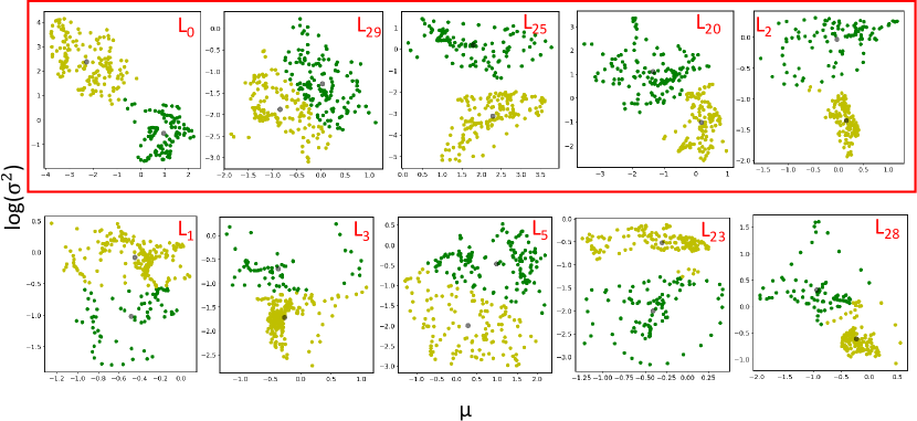
Figure 10. Scatter plots of individual latent variables: The latent distributions of the selected latent variables (highlighted in red) as compared to $5$ other latent variables that were not selected. Yellow points represent the distributions of the train images, and the green points represent the distributions of the test images that were ood. The selected latent variables into a well-formed cluster, and there is a higher separation between the train and the test image clusters. The un-selected latent variables do not form clean clusters. Using the $5$ most informative latent variables for detection resulted in better robustness and minimum sensitivity as compared to using all the latent variables as shown in Table 3. Plot axis: x-axis represents the mean of the latent distributions in the range $[-5,5]$, and the y-axis represents the log of variance in the range $[-5,5]$.

5.3. OOD Detection Results from CARLA Simulation

5.3.1. Evaluation Metrics

(1) Precision (P) is a fraction of the detector identified anomalies that are real anomalies. It is defined in terms of true positives (TP), false positives (FP), and false negatives (FN) as $TP\div(TP+FN)$. (2) Recall (R) is a fraction of all real anomalies that were identified by the detector. It is calculated as $TP\div(TP+FP)$. The FP and FN for the test scenes is shown in Table 4. (3) F1-score is a measure of the detector’s accuracy that is computed as $2\times(P\times R)\div(P+R)$. (4) Execution Time is computed as the time the detector receives an image to the time it computes the log of martingale. (5) Average latency is the number of frames between the detection and the occurrence of the anomaly. (6) Memory Usage is the memory utilized by the detector.

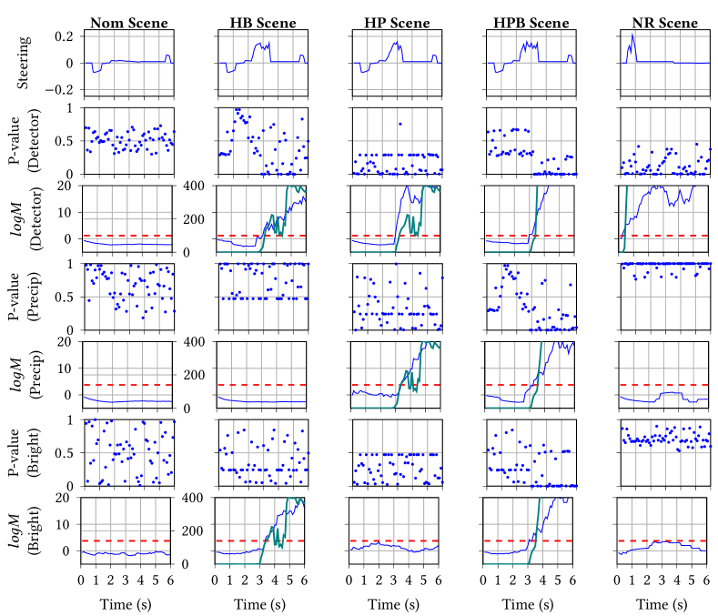
Figure 11. Runtime ood Detection: Performance of the bvae detector for the $5$ test scenes generated in Section 5.1. The solid blue line represents the log of martingale, the solid green lines represent the cusum values and the dotted red lines represent the threshold ($\tau$) for cusum comparison. Further, the left y-axis shows the log of martingale with range $[-5,20]$, and the right y-axis shows the cusum value with range $[0,400]$. The cusum threshold represented in the red dotted lines are plotted to the right y-axis.

5.3.2. Runtime OOD Detection

We evaluate the performance of the selected bvae network ($\beta=1.4$ and $n=30$) for the $5$ test scenes described in Fig. 8. Additional hyperparameters that were used by the detectors and the reasoners are as follows. The martingale sliding window size $M=20$, the cusum parameters for the detector are $\omega_{d}=14$ and $\tau_{d}=100$, and for the reasoners are $\omega_{r}=18$ and $\tau_{r}=130$. These hyperparameters were selected empirically based on the false positive results from several trial runs. Fig. 11 summarizes the detector’s performance for a short segment of the $5$ test scenes. For the $HP$, $HB$, $HPB$, and $NR$ scenes, the scene shifts from in-distribution to ood at $t=2$ seconds, and they are used to illustrate the detection and reasoning capability of our approach.

The $Nom$ scene has all the feature values within the training distribution, and it is used to illustrate the detector’s ability to identify in-distribution images. As seen in Fig. 11, the martingale of the detector and both the reasoners remain low throughout. In $HP$ and $HB$ scenes, the precipitation and the brightness feature values increase out of the training distribution at $t=2$ seconds. In the $HP$ scene, the martingales of the detector and the reasoner for the precipitation feature increase above the threshold after $t=2$ seconds. However, as seen martingale of the reasoner for brightness does not increase. So, we conclude that the precipitation feature is the reason for the ood. In the $HB$ scene, the martingales of the detector and the reasoner for the brightness feature increase above the threshold after $t=2$ seconds. Also, the martingale of the reasoner for precipitation shows a slight variation but does not increase above the threshold. So, we conclude the brightness feature is the cause of the ood. In the $HPB$ scene, the precipitation and brightness feature increase to a value out of the training distribution at $t=2$ seconds. The martingale of the detector and both the feature reasoners increase above the threshold. So, we attribute both the features to be the cause of the ood. The peaks in the steering plots at $t=2$ seconds are when the DAVE-II dnn steering predictions get erroneous, and the decision manager arbitrates the control to the autopilot controller.

The $NR$ scene is of interest for this work, as the scene has a new road segment with different background artifacts (e.g., buildings, traffic lights) that were not in the training distribution. But the precipitation and brightness feature values were within the training distribution. When tested on this scene, the detector martingale instantly increases above the threshold, identifying the scene to be ood. However, the martingales of the reasoners for precipitation and brightness only show slight variations without increasing beyond the threshold. The result implies that the scene is ood, but a feature other than brightness and precipitation has varied and is responsible for the ood.

Further, Fig. 12 shows the plots of the capability of the bvae detector in identifying changes in the current test image as compared to the previous images in the time series (problem2). For these evaluations, we used the $Nom$, $HB$, and extended $HB$ test scenes, which had a length of $50$ seconds each. The $Nom$ and $HB$ scenes are same as the previous setup, but in the extended $HB$ scene, the brightness feature value abruptly increases only for a brief period between $9.5$ seconds and $29.5$ seconds. For these test scenes, we performed the moving average calculation on a sliding window of $M=20$ with the cusum parameters of $\omega_{cp}=0.75$ and $\tau_{cp}=1.2$. With these parameters, our detector could identify change points with a short latency of $11$ frames, which translates to one second of inference time for the av system.

Figure 12. Runtime Change Detection: Moving Average and cusum for identifying feature changes in $Nom$, $HB$, and an extended $HB$ test scenes. (Left) $Nom$ scene - there is no change in the scene, so the average kl remains below $\tau$. (Center) $HB$ scene - the brightness of the scene changes at $17.5$ seconds and this was identified by the detector. (Right) Extended $HB$ scene - high brightness is introduced for a short period between $9.5$ seconds to $29.5$ seconds, and the detector was able to identify both the changes.

5.3.3. Evaluating the Design Approach

Table 3 illustrates how the proposed heuristics in each step of our approach (Section 4) results in achieving the best detector properties (text highlighted in green). The properties of interest are robustness, minimum sensitivity, and resource efficiency, which are defined in Section 2. We evaluate robustness on the in-distribution scene $Nom$, and two ood scenes $HPB$ and $NR$. The $HP$ and $HB$ scenes had variations in either the precipitation value or the brightness value, but they did not have simultaneous variations in both. So, it was suitable to use them to measure the detector’s minimum sensitivity towards these features. However, in the $HPB$ scene, both these features varied simultaneously, so it was not suitable for measuring the minimum sensitivity. The resource efficiency was measured across all the scenes. For these evaluations, we have compared the proposed heuristics to an alternate technique in each step. The comparisons are as follows (proposed techniques are underlined): (1) MIG vs. ELBO loss function (discussed in Section 3), (2) bo vs. Grid and Random Search, and (3) Selective vs. All latent variables for detection. Our evaluations are as follows.

Design-time steps of our approach				Detector Properties
	Latent Space Encoding
Partitioning	Objective Function	Optimization Algorithm	Selected $\mathcal{L}_{d}$ for Detection	Robustness F1-score (%)	Minimum Sensitivity (%)	Execution Time (ms)
		BO (30,1.4)	[0,2,20,25,29]	96.98	96	74.09
		Grid (30,1.4)	[0,2,20,25,29]	96.98	96	74.09
	MIG	Random (40,1.5)	[0,17,6,8,7]	80.75	35	79.15
		BO (30,1.0)	[0,1,6,21,23]	95.83	63	75.39
		Grid (40,1.0)	[13,28,26,23,0]	84.65	54	78.85
Yes	ELBO	Random (30,1.2)	[10,14,21,22,26]	94.9	71	74.98
		BO (30,1.0)	All 30	85.89	73	379.47
		Grid (40,1.0)	All 40	68.96	42	488.85
No	ELBO	Random (30,1.2)	All 30	89.73	53	396.89

Table 3. Design Approach Evaluation: Evaluations of how the heuristics of our design approach influence the detector properties discussed in Section 2. We evaluated Robustness on the $Nom$, $HPB$, and $NR$ scenes. Minimum sensitivity was evaluated on the $HP$ and $HB$ scenes. Resource efficiency was measured across all the test scenes. The numbers in the optimization algorithm column indicate the selected hyperparameters. Text in green highlights the best detector properties achieved by our approach. Text in red highlights a high detection time.

If the dataset can be partitioned, either mig or elbo can be used as the objective function with the bo, grid, or random search algorithms. Since the dataset can be partitioned, the latent variable heuristic could be applied to select a subset of latent variables, which can be used for detection. As illustrated in Table 3, the optimization algorithm and objective function combinations resulted in $5$ different bvae networks and $5$ latent variables for $\mathcal{L}_{d}$. Among these, the bo and grid algorithms using mig resulted in the best detector that had robustness of $96.98\%$, minimum sensitivity of $96\%$, and a detection time of $74.09$ milliseconds. In comparison, the other detectors had low robustness and minimum sensitivity, and a similar detection time.

However, if the dataset cannot be partitioned, then elbo is the only objective function that can be used with the bo, grid, or random search algorithms. However, without partitioning, the latent variable mapping heuristic cannot be applied. So, all the latent variables for the chosen bvae had to be used for detection. Using all the latent variables for detection resulted in a less robust and sensitive detector that took an average of $400$ milliseconds (text in red) as shown in Table 3.

5.4. Detection Results from Competing Baselines

We compare the performance of the bvae detector to other state-of-the-art approaches using our av example in CARLA. The approaches that we compare against are: (1) Deep-SVDD one-class classifier; (2) vae based reconstruction classifier; (3) chain of one-class Deep-SVDD classifiers; and (4) chain of vae based reconstruction classifiers. The vae network architecture is the same as that of bvae (described in Section 5) but uses the hyperparameters of $\beta=1$ and $n=1024$. The one-class Deep-SVDD network has four convolutional layers of 32/64/128/256 with $5x5$ filters with LeakyReLu activation functions and $2x2$ max-pooling, and one fully connected layer with 1568 units. These networks are also trained using a two-learning scheduler, with $100$ epochs at a learning rate $\eta$ = $1$ x $10$^$-4$, and $50$ epochs at a learning rate $\eta$ = $1$ x $10$^$-5$. Further, we combined two of these classifiers to form a chain of Deep-SVDD classifiers and a chain of vae classifiers. In each chain, one classifier is trained to classify images with variations in the values of the brightness feature, and the other is trained to classify images with variations in the values of the precipitation feature. These classifiers are combined using an OR operator.

For these evaluations, we set resource limits on the python software component (See Fig. 7) for evaluating the processing time and memory usage. We assigned a soft limit of one CPU core and a hard limit of four CPU cores on each of the components to mimic the settings of an NVIDIA Jetson TX2 board. Further, to measure the memory usage, we used the psutil (Rodola, 2016) cross-platform library.

5.4.1. Comparing Runtime ood Detection

The false positive and false negative definitions for the $HP$, $HB$, $HPB$, and $NR$ test scenes are defined in Table 4. Based on these definitions, the precision and recall of the different detectors for the test scenes are shown in Fig. 13. In $HP$ and $HB$ scenes, a single feature (precipitation or brightness) value was varied, and the classifier that was not trained on the representative feature of that scene had low true positives. So, the precision and recall of these detectors are mostly zero. In the $HPB$ scene shown in Fig. 13-c, both the features were varied, so a single one-class classifier was not sufficient to identify both the feature variations. However, the one-class classifier chains with an OR logic had higher precision in detecting the feature variations in all these scenes. Similarly, the detection and ood reasoning capability of the bvae detector could identify both the feature variations.

For the $NR$ scene shown in Fig. 13-d, which had a new road segment with the precipitation and brightness values within the training distribution, both the one-class classifiers and their chains raise a false alarm. So, their precision towards detecting variations in these features is low (roughly $1\%$). In contrast, the bvae detector alongside the reasoner was able to identify that the ood behavior was not because of the precipitation and brightness with a precision of $46\%$. These results imply that the bvae detector can precisely identify if the features of interest are responsible for the ood. Whereas a similar reasoning inference cannot be achieved using the other approaches.

Scene	FP	FN
$HP$	The image is not OOD due to high precipitation, but it is identified as OOD.	The image is OOD due to high rain, but is identified as in-distribution
$HB$	The image is not OOD due to high brightness, but is identified as OOD.	The image is OOD due to high brightness, but is identified as in-distribution.
$HPB$	The image is not OOD due to high precipitation and high brightness but, is identified as OOD.	The image is OOD due to high rain and high brightness, but is identified as in-distribution.
$NR$	The image is not OOD due to change in road segment, but is identified as OOD.	The image is OOD due to change in road segment, but is identified as in-distribution.

Table 4. Metrics: Definitions of false positives and false negatives for the $HP$, $HB$, $HPB$, and $NR$ test scenes.

Figure 13. Precision and Recall: Evaluations on different scenes: (a) $HP$ - top left, (b) $HB$ - bottom left, (c) $HPB$ - top right and (d) $NR$ - bottom right. The detectors compared are: $SD1$ - Deep-SVDD Precipitation detector, $SD2$ - Deep-SVDD brightness detector, $SDC$ - Deep-SVDD detector chain, $VD1$ - vae Precipitation detector, VD2 - vae brightness detector, VDC - vae detector chain, BD - bvae detector. These values were collected by running the detectors on each scene for 20 times.

5.4.2. Comparing Execution Time and Latency

To emulate a resource constrained setting, we performed the evaluation for execution time and latency on one CPU core.

Execution Time: As discussed earlier, we selected $5$ latent variables for detection and one latent variable each for reasoning about the precipitation and brightness features. Two components that mainly contribute to the execution time of the bvae detector are: (1) the time taken by the bvae’s encoder to generate the latent variables, and (2) the time taken by ICP and martingale for runtime detection. The average execution time using all $30$ latent variables of the bvae was $400$ milliseconds, and this was drastically reduced to $74.09$ milliseconds when the $5$ selected latent variables were used. Also, the reasoner only took about $9$ milliseconds as it worked in parallel to the detector.

In comparison, the Deep-SVDD classifiers took an average of $41$ milliseconds for detection, and its chain took an average of $43.36$ milliseconds, as shown in Fig. 14. Also, each of the vae based reconstruction classifiers took an average of $53$ milliseconds for detection, and its chain took an average of $57$ milliseconds. The Deep-SVDD and vae based reconstruction classifiers performed slightly faster than our detector.

Figure 14. Timing Analysis:(Left) Execution Time in milliseconds and (Right) Detection latency in number of frames, of the different detectors for the $HP$, $HB$, $HPB$ and $NR$ scenes. The detectors are $SD1$ - Deep-SVDD Precipitation detector, $SD2$ - Deep-SVDD brightness detector, $SDC$ - Deep-SVDD detector chain, $VD1$ - vae Precipitation detector, $VD2$ - vae brightness detector, $VDC$ - vae detector chain, $BD$ - bvae detector. These values were collected by running the detectors on each scene for 20 times.

Detection Latency: The detection latency in our context is the number of frames between the detection and the occurrence of the ood. In our approach, the latency is dependent on the size of the martingale window, which is dependent on the cps dynamics and the sampling period of the system as discussed in Section 3.4. In addition, the selection of the cusum threshold also impacts the latency. In these experiments, our av traveled at a constant speed of 0.5 m/s, so we used a fixed window size of 20 images. Further, we empirically selected the cusum threshold to be $100$. With this configuration, the bvae detector had an average latency of $12.6$ frames, and the reasoners had an average latency of about $11.5$ frames across the $4$ test scenes. In comparison, the Deep-SVDD classifiers and their chain had an average latency of $11$ frames and $11.21$ frames, respectively. Also, each of the vae based reconstruction classifiers and their chain had an average latency of $13$ frames and $12.9$ frames, respectively.

To summarize, all the approaches had similar detection latency, with the Deep-SVDD classifier performing slightly better. The Deep-SVDD classifier and its chain had slightly shorter latency as compared to our detector. However, the bvae detector had a lower latency compared to the vae based reconstruction classifier and its chain.

5.4.3. Comparing Memory Usage

Our approach uses a single bvae network to perform both detection and reasoning. Specifically, we only utilize the network’s encoder instead of both the encoder and the decoder. The average memory utilization of the bvae detector was $2.49$ GB, and the reasoners were $0.23$ GB. In comparison, the Deep-SVDD classifiers and their chain utilized an average memory of $3.2$ GB and $6.4$ GB, respectively. Also, the vae based reconstruction classifiers and their chain utilized an average memory of $3.6$ GB and $7.2$ GB, respectively. The classifier chains utilized higher memory because two dnns were used for detection.

To summarize, our approach utilizes lesser memory because: (1) it only requires the encoder of a single bvae network for both detection and reasoning; and (2) it utilizes fewer latent variables for detection because it relies on the disentanglement concept. For the av example, our detector only required $5$ latent variables as compared to $1024$ latent variables of the vae reconstruction classifier and $1568$ activation functions in the embedding layer of the Deep-SVDD classifier.

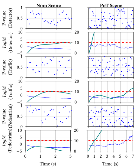
Figure 15. Runtime ood Detection on nuImages dataset: Performance of the bvae detector for the $Nom$ (nominal) and $PoT$ (pedestrian or traffic) scenes of the nuImages experiments. For the martingale plots, the solid blue line represents the log of martingale, the solid green lines represent the cusum values and the dotted red lines represent the threshold ($\tau$) for cusum comparison. Further, the left y-axis shows the log of martingale with range $[-5,10]$, and the right y-axis shows the cusum value with range $[0,20]$. The cusum threshold represented in the red dotted lines are plotted to the right y-axis.

5.5. ood Detection Results from nuImages dataset

As the second example, we apply our detection approach on a small fragment of the nuImages (nuscenes, [n.d.]) dataset. We report the preliminary results of our evaluation in this section.

Dataset Overview: The nuImages dataset is derived from the original nuScenes dataset (Caesar et al., 2020). The nuImages dataset provides image annotation labels, reduced label imbalance, and a larger number of similar scenes (e.g., a scene with the same road segment but different time-of-day, weather, and pedestrian density values), which makes it suitable for our work. The dataset has $93,000$ images collected at $2Hz$, and it has annotations for foreground objects such as vehicles, animals, humans, static obstacles, moving obstacles, etc. The foreground objects further have additional attributes about the weather, activity of a vehicle, traffic, number of pedestrians, pose of the pedestrians, among others. We demonstrate our ood detection capability on scenes with different values of traffic and pedestrian density features. For these experiments, we train the detector with different traffic and pedestrian values and then used it to detect images in which either traffic or pedestrian features are absent (ood condition).

Data Partitioning: The training set $\mathcal{T}$ had images from $4$ scenes with varying traffic and pedestrian values. We partitioned $\mathcal{T}$ into two partitions. $P1$ had images with medium and high pedestrian density values in the range $[1,5]$ and more than $5$, respectively. $P2$ had images with medium and high traffic values in the range $[1,5]$ and more than $5$, respectively. The test scenes for this evaluation were nominal ($Nom$) and a pedestrian or traffic ($PoT$) scene. The $Nom$ scene was in distribution, and it had $30$ images in time series captured on a sunny day from a road segment in Singapore city with traffic and pedestrians in the training distribution range. The $PoT$ scene had $70$ images in time series captured from a similar road segment, and it either had traffic or pedestrians, but not both together. For most images in this scene, the traffic density took a value in the training range, but the pedestrian value was close to zero. Further, our test scenes were short as it was difficult to find longer image sequences that belonged to a sunny day and similar road segment.

Detector Design: We applied our approach discussed in Section 4 and we used the same bvae network structure as discussed in Section 5.2. Using this set up, we selected a bvae network with hyperparameters $n$=30 and $\beta$=1.1, that resulted in the maximum mig of $0.0006$. We then identified the detector latent variable set $\mathcal{L}_{d}$ to be $\{L_{0},L_{7},L_{9},L_{22}\}$. Further, we selected latent variables $L_{9}$ and $L_{22}$ as the reasoners for the traffic density and pedestrian density partitions, respectively.

ood Detection: For runtime ood detection, we used a window size $M$=30 for martingale computation and $\omega$=2 and $\tau$=10 for reasoners and detector cusum calculations. The p-value and martingale plots for detection and reasoning are shown in Fig. 15. The detector Martingale for $Nom$ test scene remained low, and all in-distribution images were detected as in-distribution. The martingale of the traffic density reasoner remained low for most images except for $2$ images. We hypothesize the reason for this could be that the vehicle and background blended well that confused the reasoner. The martingale of the pedestrian reasoner remained low throughout the scene. For OOD scene $PoT$, the detector identified $92\%$ ($65/70$) of the images correctly as OOD. However, the first $5$ images were incorrectly detected to be in-distribution because of the detection latency of our window-based martingale approach. Also, as the traffic density was mostly zero throughout the scene, the martingale of traffic density reasoner is mostly flat throughout. But, for pedestrian reasoner, all the images were identified as OOD except the first $9$ images. The false negatives are primarily because of the complexity of images in a scene and the detection latency. After these images, the martingale increases, and the cusum also increase above its threshold. In summary, the reasoners worked reasonably well for these scenes but had a slow martingale growth because of several background attributes like sun glare, trees, and traffic lights.

Challenges: We discuss the several challenges of applying our approach to a real-world dataset. The first challenge is the existence of time series images. Although the nuImages dataset provides the notion of a scene, they contain time gaps, especially after partitioning them into train and test the dataset. Second, the labels provided for the dataset images are coarse grain. For example, in nuImages dataset, the semantic label annotations are only limited to high-level foreground objects like pedestrian and cars, and extracting these labels requires significant pre-processing. Another challenge is the complexity of images in real-world datasets. The presence of excess background information such as trees, traffic signals, shadow, reflections, among others, makes the real-world images complex, and it also impacts the information in the latent space. The other challenge is the absence of scenes in which the feature(s) gradually change their values. This makes it difficult to apply our latent variable mapping. Further, finding similar scenes with variations in the specific feature(s) of interest is difficult. For our experiments, we had to perform significant pre-processing to extract short image sequences to perform ood detection and reasoning.

5.6. Discussion

With dnn being widely used in perception pipelines of automotive cps, there has been an increased need for ood detectors that can identify if the operational test image to the dnn is in conformance to the training set. Addressing this problem is challenging because these images have multiple feature labels, and a change in the value of one or more features can cause the image to be ood. This problem is commonly solved using a multi-chained one-class classifier with each classifier trained on one feature label. However, as shown by our evaluation in Section 5.4, the chain gets computationally expensive with an increased number of image features. So, we have proposed a single bvae detector that is sensitive to variations in multiple features and is computationally inexpensive in comparison to the classifier chains. For example, to perform detection on a real-world automotive dataset like nuScenes with $38$ semantic labels, a multi-chained vae based reconstruction classifier (discussed in our experiments) would require training $38$ different vae dnns as compared to a single bvae detector that is presented in this work. A memory projection based on the results in Section 5.4.3 is shown in Fig. 16. It shows that the multi-chain classifier will need a memory of $136.8$ GB. In comparison, our approach requires a single network with one or a few latent variables for detection on each label, and this requires only $10.96$ GB of memory.

Figure 16. Memory Overhead: Predicted memory usage of a vae based reconstruction chain and a single $\beta$-VAE detector for the nuScenes images. If a vae reconstruction detector is used for each of the $38$ nuScenes labels, then the memory usage would linearly grow to $136.8$ GB. However, a bvae detector based on our approach would only require $10.96$ GB. These values were computed based on results in Section 5.4.3.

Another related problem motivated in this work is the ood reasoning capability to identify the most responsible feature(s). The reasoning capability is desirable for the system to decide on the mitigation action it must perform. For example, if the detector can identify a high traffic feature to be the cause of the ood, then the system can switch to an alternate controller with lower autonomy. This reasoning capability cannot be achieved using the state-of-the-art chain of one-class classifiers. But the bvae detector designed and trained using our approach is sensitive to variations in multiple features. We have evaluated this capability of the bvae detector by applying it to several ood scenes in CARLA simulation (see Fig. 11). Especially the $NR$ scene that had a new road segment and background artifacts that are not in the training set. In this scene, the multi-chained network identified the scene to be ood because of the precipitation and brightness features. In comparison, our detector’s ood reasoning capability was able to identify with a precision of $46\%$ that the cause was not precipitation or brightness.

In addition to the reasoning capability, a detector for a multi-labeled dataset should have minimum sensitivity (defined in Section 2) towards all the feature labels. High minimum sensitivity is needed to detect variations in all the feature labels of the training set images. In our approach, we hypothesize that using the most informative latent variables can provide good minimum sensitivity for the detector towards each feature label. We back this by our results in Table 3, which illustrates that a detector that used the $5$ most informative latent variables had a high minimum sensitivity to variations in both the precipitation and brightness features (highlighted in green text in the Table). In comparison, the detectors that used all the latent variables for detection had lower minimum sensitivity, as illustrated in the Table.

Besides identifying if the input images are ood to the training data, it is necessary to check if they have changed compared to the previous sequence of images in the time series. Such abrupt changes in the current input will increase the system’s risk of consequence (e.g., collision) (Hartsell et al., 2021), so it is critical to detect them. This problem is necessary to be addressed but has not been given much importance in the ood detection literature. In this work, we use the detector’s latent variables in a moving window based on cusum for detecting abrupt changes in the features of the operational test images. We validated our approach across $3$ different scenes (see Fig. 12) for which our detector could accurately identify feature variations with a short latency of about $11$ frames.

Finally, in designing ood detectors for cps, one needs to take into consideration of the system’s dynamics. But this is often not given importance in the existing detection approaches. Only recently, Cai et al. (Cai and Koutsoukos, 2020) have proposed an ood detection mechanism on time series images that consider the system dynamics. As discussed in Section 4.4, we rely on their icp and martingale framework approach for runtime detection over a short sliding window of images. The sliding window size needs to be adjusted based on the operational system dynamics like runtime sampling rate and the speed at which the system is traveling.

6. Related Work

There has been significant ongoing research to handle the brittleness and susceptibility of dnns. We have grouped the existing approaches into different classes and briefly discuss them below.

Domain Adaptation involves transferring knowledge between a labeled source domain and an unlabeled target domain  (Pan and Yang, 2009). The key idea is to learn domain invariant features of the training data by providing less importance to dataset biases. This is also referred to as transductive transfer learning and is used when the train and the target tasks remain the same while the domains are different. Altering the dnn structure has been one of the approaches that have been used for feature transferability. One such example is the Deep Adaptation Network (DAN) (Long et al., 2015) that allows for feature transferability in the task specific layers of dnn network while reducing domain related information. Biasing the training objective to learn the domain invariant feature(s) has been the other widely adopted approach. For example, Heinze-Deml et al. (Heinze-Deml and Meinshausen, 2021) proposes a conditional variance penalty-based training loss function to learn domain invariant features. Although domain adaptation has been widely used, an assumption on the prior distributions of target domains is restrictive for practical applications like cps (Volpi et al., 2018). Further, negative transfer of knowledge between the source and target domains has been a common problem (Wang et al., 2019).

Confidence Estimation involves estimating the confidence in the inputs to a dnn. There have been several approaches to estimating confidence. The first approach involves adding a confidence branch at the logits before the softmax layer  (DeVries and Taylor, 2018). The second approach involves using Bayesian Networks for representing uncertainties in the dnn  (MacKay, 1992; Neal, 2012). Ensembles of dnn have been another approach used for estimating the confidence in the inputs  (Lakshminarayanan et al., 2017; Geifman et al., 2018). All these approaches mostly require making changes to the dnn or will require training model ensembles. Recently,  Jha et al.  (Jha et al., 2019) have proposed the attribution based confidence (ABC) metric that does not require access to training data or does not need training model ensembles. It is computed by sampling in the neighborhood of high-dimensional data and then computing a score for its conformance. The metric looks robust, and it does not require access to the training data at runtime, which is an advantage compared to our approach. But the impact of input feature correlations and interactions on the attribution over features require future investigation  (Sundararajan et al., 2017).

Identifying Distribution Shifts involves identifying if the test observation has shifted from the training distribution. Probabilistic classifiers like gan and vae have been widely adopted for identifying shifts in the test observations  (Ruff et al., 2018; Cai and Koutsoukos, 2020; Denouden et al., 2018; An and Cho, 2015). Our work belongs to this class, and different approaches in this class are discussed in Section 6.1.

In contrast to these approaches, we formulate the problem as a multi-label ood detection problem, and in addition to identifying an ood condition, we also find the feature(s) causing it.

6.1. Probabilistic One-class Classifiers

6.1.1. Adversarial Networks

gan have emerged as the leading paradigm in performing un-supervised and semi-supervised tasks like classification and ood detection  (Akcay et al., 2019; Zenati et al., 2018). gan has been shown to outperform classical ood techniques on benchmark datasets  (Zenati et al., 2018). This network is used along with an adversarial training loss function to perform unsupervised ood detection  (Akcay et al., 2019). Further, Adversarial Variational Bayes (AVB), a training technique to improve the inference model of vae  (Mescheder et al., 2017). It combines vae and gan to rephrase the maximum-likelihood problem of the vae as a two player game. Although gan has performed well in detecting ood data, there are several problems in using them  (Creswell et al., 2018; Vu et al., 2019). These problems are (1) training complexity because of the instability between the generator and discriminator networks, and (2) mode collapse problem that results in the generator only producing similar samples or, in the worst-case only a single sample.

Adversarial Autoencoder (Makhzani et al., 2015) is a probabilistic network that uses the reconstruction capability of an autoencoder along with the adversarial training procedures of a gan. For example, the reconstruction error is combined with the likelihood in the latent space to perform anomaly detection  (Beggel et al., 2019). Vu, Ha Son et al.  (Vu et al., 2019) have proposed a Dual Adversarial Autoencoder network that uses two autoencoders and discriminators to perform anomaly detection. However, training Adversarial Autoencoders is expensive as it requires training both the autoencoder network and the adversarial network.

6.1.2. Variational Autoencoders (VAE)

vae is the other unsupervised probabilistic generative model that has been used because of its capability to learn latent space of the input data  (Kingma and Welling, 2013). The latent variables generated by these models are used to learn the correlation between the features of the input data  (Liu et al., 2019). The vae based ood approaches can be classified into two categories.

Reconstruction based techniques use the normalized difference between each point of the input data ($x$) and the reconstructed data ($x^{\prime}$) generated by a vae. For example, the authors in  (Richter and Roy, 2017; Cai and Koutsoukos, 2020) have used the pixel-wise mean square distance between the input image and the reconstructed image as the metric for anomaly detection. As an extension, the reconstruction probability that uses the stochastic latent variables of vae has been used to compute a probabilistic anomaly score  (An and Cho, 2015). Although being widely used, this approach can be error-prone when the ood samples lie on the boundary of the training distribution  (Denouden et al., 2018).

Latent space based techniques use distance and density-based metrics on the latent space generated by the encoder of vae to detect ood observations. For example, Denouden et al.  (Denouden et al., 2018) compute the Mahalanobis distance between the latent distributions of the test image and the mean vector of the images in the training set, which is also combined with the reconstruction loss to detect ood images. The authors in  (Vasilev et al., 2020) evaluate the latent space with different metrics like Euclidean distance and Bhattacharyya distance for ood detection. Although being used for ood detection  (Denouden et al., 2018; Vasilev et al., 2020), there is a known problem, that the generated latent variables are unstructured, entangled, and lack the ease of understanding  (Klys et al., 2018). To address this problem, there has been significant research in structuring and disentangling the latent space  (Bengio et al., 2013; Higgins et al., 2016; Chen et al., 2018; Mathieu et al., 2019), which is discussed in the following section.

6.2. Disentangling Latent Representations

Learning a disentangled latent space have been shown to be beneficial for several tasks like pose invariant face recognition  (Tran et al., 2017; Peng et al., 2017), video predictions  (Hsieh et al., 2018), and anomaly detection  (Wang et al., 2020). While there are several approaches to learning a disentangled latent space  (Bengio et al., 2013), of particular interest to this work are approaches that use the vae structure. Recently, variants of a vae like FactorVAE  (Kim and Mnih, 2018), bvae  (Higgins et al., 2016), and $\beta$-TCVAE  (Chen et al., 2018) have been used. Among these, bvae has been widely used because it provides a single $\beta$ gating hyperparameter that can be used control the latent space disentanglement  (Higgins et al., 2016). Mathieu, Emile et al.  (Mathieu et al., 2019) illustrates that a bvae generates a lower overlap of the latent variables as compared to the original vae, and illustrates how different values of $\beta$ impacts the latent variable overlap. Further, Locatello et al.  (Locatello et al., 2019) have illustrated with experiments that network inductive biases are necessary to achieve unsupervised disentanglement.

In recent years bvae is used for ood detection tasks because of its ability to generate a disentangled latent space. In our previous work  (Sundar et al., 2020), we have used the tuning capability of a bvae to make it sensitive to different image features (e.g., traffic density, pedestrians) and then used it to detect changes in those features. Graydon et al.  (Graydon and Sahin, 2018) have used the latent variables generated by a bvae along with Gaussian mixture models to identify ood on cancer datasets. A combination of the reconstruction error and the distances among the latent variables of a bvae is used as the anomaly score  (Li, 2020). Further, a bvae is shown to perform better for anomaly detection on MRI datasets as compared to a classical vae  (Zhou et al., 2020). However, these approaches either randomly select the $\beta$ values or manually tune them, which can be expensive and time consuming. In contrast, our work provides a bo based heuristic to select the $\beta$ value.

Further, to measure the level of disentanglement, several methods and metrics are available. Visualization of reconstructions by inspecting latent traversals has been a simple method that has been widely used. But visualization alone is not sufficient, as discussed in Section 1. So, several qualitative and quantitative metrics have been proposed for this task. A classifier based supervised learning metrics  (Higgins et al., 2016; Kim and Mnih, 2018; Grathwohl and Wilson, 2016) have been designed when all the underlying generative factors of an image are known. For example, the BetaVAE metric (Higgins et al., 2016) builds a linear classifier that predicts the index of a fixed factor with variations. However, this metric has a drawback of axis alignment, and this is overcome by the FactorVAE metric  (Kim and Mnih, 2018) by using a majority vote classifier. Also, these metrics require building and tuning the sensitivity of the classifiers, which is difficult to design and train. This problem is overcome by the mig  (Chen et al., 2018) metric, which is a quantitative metric based on the mutual information between the features and latent variables. In this work, we have used mig to measure the level of latent space disentanglement.

7. Conclusions and Future Work

In this paper, we proposed a design approach to generate a partially disentangled latent space and learn an approximate mapping between the latent variables and features for ood detection and reasoning. To generate the disentangled latent space, we use a bvae network and tune its hyperparameter ($n$, $\beta$) using a bo heuristic. Next, we perform a latent variable mapping to identify the most informative latent variables for detection and identify latent variable(s) which are sensitive to specific features and use them for reasoning the ood problem. We evaluated our approach using an av example in the CARLA simulation and illustrated the preliminary results from the nuImages dataset. Our evaluation has shown that the detector designed using our approach has good robustness, minimum sensitivity, and low execution time. The detector could also detect ood images and identify the most likely feature(s) causing it.

Future extensions and applications of the proposed approach include: (1) improving the latent variable mapping heuristic to perform robust correspondence between the features and latent variables, (2) explore alternate metrics such as Wasserstein distance for latent variable mapping, (3) apply the approach to real-world datasets and research cps testbeds like DeepNNCar  (Ramakrishna et al., 2020), and (4) use the anomaly detection results to perform higher-level decision making such as controller selection or enactment of contingency plans.

References

- (1)
- Akcay et al. (2019) Samet Akcay, Amir Atapour-Abarghouei, and Toby P. Breckon. 2019. GANomaly: Semi-supervised Anomaly Detection via Adversarial Training. In Computer Vision – ACCV 2018, C. V. Jawahar, Hongdong Li, Greg Mori, and Konrad Schindler (Eds.). Springer International Publishing, Cham, 622–637.
- An and Cho (2015) Jinwon An and Sungzoon Cho. 2015. Variational autoencoder based anomaly detection using reconstruction probability. Special Lecture on IE 2, 1 (2015), 1–18.
- Basseville et al. (1993) Michèle Basseville, Igor V Nikiforov, et al. 1993. Detection of abrupt changes: theory and application. Vol. 104. prentice Hall Englewood Cliffs.
- Beggel et al. (2019) Laura Beggel, Michael Pfeiffer, and Bernd Bischl. 2019. Robust anomaly detection in images using adversarial autoencoders. In Joint European Conference on Machine Learning and Knowledge Discovery in Databases. Springer, 206–222.
- Bengio et al. (2013) Yoshua Bengio, Aaron Courville, and Pascal Vincent. 2013. Representation learning: A review and new perspectives. IEEE transactions on pattern analysis and machine intelligence 35, 8 (2013), 1798–1828.
- Bojarski et al. (2016) Mariusz Bojarski, Davide Del Testa, Daniel Dworakowski, Bernhard Firner, Beat Flepp, Prasoon Goyal, Lawrence D Jackel, Mathew Monfort, Urs Muller, Jiakai Zhang, et al. 2016. End to end learning for self-driving cars. arXiv preprint arXiv:1604.07316 (2016).
- Caesar et al. (2020) Holger Caesar, Varun Bankiti, Alex H Lang, Sourabh Vora, Venice Erin Liong, Qiang Xu, Anush Krishnan, Yu Pan, Giancarlo Baldan, and Oscar Beijbom. 2020. nuscenes: A multimodal dataset for autonomous driving. In Proceedings of the IEEE/CVF conference on computer vision and pattern recognition. 11621–11631.
- Cai and Koutsoukos (2020) Feiyang Cai and Xenofon Koutsoukos. 2020. Real-time out-of-distribution detection in learning-enabled cyber-physical systems. In 2020 ACM/IEEE 11th International Conference on Cyber-Physical Systems (ICCPS). IEEE, 174–183.
- Chen et al. (2018) Tian Qi Chen, Xuechen Li, Roger B Grosse, and David K Duvenaud. 2018. Isolating sources of disentanglement in variational autoencoders. In Advances in Neural Information Processing Systems. 2610–2620.
- Creswell et al. (2018) Antonia Creswell, Tom White, Vincent Dumoulin, Kai Arulkumaran, Biswa Sengupta, and Anil A Bharath. 2018. Generative adversarial networks: An overview. IEEE Signal Processing Magazine 35, 1 (2018), 53–65.
- Dejanović et al. (2017) Igor Dejanović, Renata Vaderna, Gordana Milosavljević, and Željko Vuković. 2017. TextX: a python tool for Domain-Specific Languages implementation. Knowledge-Based Systems 115 (2017), 1–4.
- Denouden et al. (2018) Taylor Denouden, Rick Salay, Krzysztof Czarnecki, Vahdat Abdelzad, Buu Phan, and Sachin Vernekar. 2018. Improving reconstruction autoencoder out-of-distribution detection with mahalanobis distance. arXiv:1812.02765 (2018).
- DeVries and Taylor (2018) Terrance DeVries and Graham W Taylor. 2018. Learning confidence for out-of-distribution detection in neural networks. arXiv preprint arXiv:1802.04865 (2018).
- Dosovitskiy et al. (2017) Alexey Dosovitskiy, German Ros, Felipe Codevilla, Antonio Lopez, and Vladlen Koltun. 2017. CARLA: An open urban driving simulator. arXiv:1711.03938 (2017).
- Dubey et al. (2011) Abhishek Dubey, Gabor Karsai, and Nagabhushan Mahadevan. 2011. Model-based software health management for real-time systems. In 2011 Aerospace Conference. IEEE, 1–18.
- Edwards (2008) Sheri Edwards. 2008. Elements of Information Theory, Thomas M. Cover, Joy A. Thomas, John Wiley & Sons, Inc.(2006). , 18 pages.
- Eski and Yildirim (2014) İkbal Eski and SCahin Yildirim. 2014. Design of neural network control system for controlling trajectory of autonomous underwater vehicles. International Journal of Advanced Robotic Systems 11, 1 (2014), 7.
- Fedorova et al. (2012) Valentina Fedorova, Alex Gammerman, Ilia Nouretdinov, and Vladimir Vovk. 2012. Plug-in martingales for testing exchangeability on-line. arXiv preprint arXiv:1204.3251 (2012).
- foretellix ([n.d.]) [Online] foretellix. [n.d.]. Open M-SDL. https://www.foretellix.com/open-language/
- Fremont et al. (2019) Daniel J Fremont, Tommaso Dreossi, Shromona Ghosh, Xiangyu Yue, Alberto L Sangiovanni-Vincentelli, and Sanjit A Seshia. 2019. Scenic: a language for scenario specification and scene generation. In Proceedings of the 40th ACM SIGPLAN Conference on Programming Language Design and Implementation. 63–78.
- Gardner et al. (2014) Jacob R Gardner, Matt J Kusner, Zhixiang Eddie Xu, Kilian Q Weinberger, and John P Cunningham. 2014. Bayesian Optimization with Inequality Constraints.. In ICML, Vol. 2014. 937–945.
- Geifman et al. (2018) Yonatan Geifman, Guy Uziel, and Ran El-Yaniv. 2018. Bias-reduced uncertainty estimation for deep neural classifiers. arXiv preprint arXiv:1805.08206 (2018).
- Goodfellow et al. (2014) Ian Goodfellow, Jean Pouget-Abadie, Mehdi Mirza, Bing Xu, David Warde-Farley, Sherjil Ozair, Aaron Courville, and Yoshua Bengio. 2014. Generative adversarial nets. In Advances in neural information processing systems. 2672–2680.
- Grathwohl and Wilson (2016) Will Grathwohl and Aaron Wilson. 2016. Disentangling space and time in video with hierarchical variational auto-encoders. arXiv preprint arXiv:1612.04440 (2016).
- Graydon and Sahin (2018) Tucker Graydon and Ferat Sahin. 2018. Novelty Detection and Analysis with a Beta-VAE Network. In 2018 IEEE International Conference on Systems, Man, and Cybernetics (SMC). IEEE, 2687–2691.
- Hartsell et al. (2021) C. Hartsell, S. Ramakrishna, A. Dubey, D. Stojcsics, N. Mahadevan, and G. Karsai. 2021. ReSonAte: A Runtime Risk Assessment Framework for Autonomous Systems. In 2021 2021 International Symposium on Software Engineering for Adaptive and Self-Managing Systems (SEAMS) (SEAMS). IEEE Computer Society, Los Alamitos, CA, USA, 118–129. https://doi.org/10.1109/SEAMS51251.2021.00025
- Hastie et al. (2009) Trevor Hastie, Robert Tibshirani, and Jerome Friedman. 2009. The elements of statistical learning: data mining, inference, and prediction. Springer Science & Business Media.
- Heinze-Deml and Meinshausen (2021) Christina Heinze-Deml and Nicolai Meinshausen. 2021. Conditional variance penalties and domain shift robustness. Machine Learning 110, 2 (2021), 303–348.
- Higgins et al. (2016) Irina Higgins, Loic Matthey, Arka Pal, Christopher Burgess, X-avier Glorot, Matthew Botvinick, Shakir Mohamed, and Alexan-der Lerchner. 2016. Beta-VAE: Learning basic visual concepts with a constrained variational framework. ICLR17 (2016).
- Hsieh et al. (2018) Jun-Ting Hsieh, Bingbin Liu, De-An Huang, Li F Fei-Fei, and Juan Carlos Niebles. 2018. Learning to decompose and disentangle representations for video prediction. In Advances in Neural Information Processing Systems. 517–526.
- Hutter et al. (2019) Frank Hutter, Lars Kotthoff, and Joaquin Vanschoren. 2019. Automated machine learning: methods, systems, challenges. Springer Nature.
- Jakab et al. (2020) Marek Jakab, Lukas Hudec, and Wanda Benesova. 2020. Partial disentanglement of hierarchical variational auto-encoder for texture synthesis. IET Computer Vision 14, 8 (2020), 564–574.
- Jha et al. (2019) Susmit Jha, Sunny Raj, Steven Fernandes, Sumit Kumar Jha, Somesh Jha, Brian Jalaian, Gunjan Verma, and Ananthram Swami. 2019. Attribution-based confidence metric for deep neural networks. (2019).
- Jones et al. (1998) Donald R Jones, Matthias Schonlau, and William J Welch. 1998. Efficient global optimization of expensive black-box functions. Journal of Global optimization 13, 4 (1998), 455–492.
- Kim and Mnih (2018) Hyunjik Kim and Andriy Mnih. 2018. Disentangling by factorising. In International Conference on Machine Learning. PMLR, 2649–2658.
- Kingma and Welling (2013) Diederik P Kingma and Max Welling. 2013. Auto-encoding variational bayes. arXiv preprint arXiv:1312.6114 (2013).
- Kingma and Welling (2019) Diederik P Kingma and Max Welling. 2019. An introduction to variational autoencoders. arXiv preprint arXiv:1906.02691 (2019).
- Klys et al. (2018) Jack Klys, Jake Snell, and Richard Zemel. 2018. Learning latent subspaces in variational autoencoders. In Advances in Neural Information Processing Systems. 6444–6454.
- Ko et al. (2017) ByungSoo Ko, Ho-Jin Choi, Chansol Hong, Jong-Hwan Kim, Oh Chul Kwon, and Chang D Yoo. 2017. Neural network-based autonomous navigation for a homecare mobile robot. In 2017 IEEE International Conference on Big Data and Smart Computing (BigComp). IEEE, 403–406.
- Kohli and Chadha (2019) Puneet Kohli and Anjali Chadha. 2019. Enabling pedestrian safety using computer vision techniques: A case study of the 2018 uber inc. self-driving car crash. In Future of Information and Communication Conference. Springer, 261–279.
- Lakshminarayanan et al. (2017) Balaji Lakshminarayanan, Alexander Pritzel, and Charles Blundell. 2017. Simple and Scalable Predictive Uncertainty Estimation Using Deep Ensembles. In Proceedings of the 31st International Conference on Neural Information Processing Systems (NIPS’17). Curran Associates Inc., Red Hook, NY, USA, 6405–6416.
- Li (2020) Xiaoyan Li. 2020. Anomaly Detection Based on Disentangled Representation Learning. Ph.D. Dissertation. Université d’Ottawa/University of Ottawa.
- Liu et al. (2019) Yang Liu, Eunice Jun, Qisheng Li, and Jeffrey Heer. 2019. Latent space cartography: Visual analysis of vector space embeddings. In Computer Graphics Forum, Vol. 38. Wiley Online Library, 67–78.
- Locatello et al. (2019) Francesco Locatello, Stefan Bauer, Mario Lucic, Gunnar Raetsch, Sylvain Gelly, Bernhard Schölkopf, and Olivier Bachem. 2019. Challenging common assumptions in the unsupervised learning of disentangled representations. In international conference on machine learning. PMLR, 4114–4124.
- Long et al. (2015) Mingsheng Long, Yue Cao, Jianmin Wang, and Michael Jordan. 2015. Learning transferable features with deep adaptation networks. In International conference on machine learning. PMLR, 97–105.
- MacKay (1992) David JC MacKay. 1992. A practical Bayesian framework for backpropagation networks. Neural computation 4, 3 (1992), 448–472.
- Makhzani et al. (2015) Alireza Makhzani, Jonathon Shlens, Navdeep Jaitly, Ian Goodfellow, and Brendan Frey. 2015. Adversarial autoencoders. arXiv preprint arXiv:1511.05644 (2015).
- Martinez-Estudillo et al. (2008) Francisco J Martinez-Estudillo, Pedro Antonio Gutiérrez, César Hervás, and Juan Carlos Fernández. 2008. Evolutionary learning by a sensitivity-accuracy approach for multi-class problems. In 2008 IEEE Congress on Evolutionary Computation (IEEE World Congress on Computational Intelligence). IEEE, 1581–1588.
- Mathieu et al. (2019) Emile Mathieu, Tom Rainforth, Nana Siddharth, and Yee Whye Teh. 2019. Disentangling disentanglement in variational autoencoders. In International Conference on Machine Learning. PMLR, 4402–4412.
- Mescheder et al. (2017) Lars Mescheder, Sebastian Nowozin, and Andreas Geiger. 2017. Adversarial variational bayes: Unifying variational autoencoders and generative adversarial networks. In International Conference on Machine Learning. PMLR, 2391–2400.
- Neal (2012) Radford M Neal. 2012. Bayesian learning for neural networks. Vol. 118. Springer Science & Business Media.
- nuscenes ([n.d.]) [Online] nuscenes. [n.d.]. nuImage dataset. https://www.nuscenes.org/nuimages
- Pan and Yang (2009) Sinno Jialin Pan and Qiang Yang. 2009. A survey on transfer learning. IEEE Transactions on knowledge and data engineering 22, 10 (2009), 1345–1359.
- Pei et al. (2017) Kexin Pei, Yinzhi Cao, Junfeng Yang, and Suman Jana. 2017. DeepXplore: Automated whitebox testing of deep learning systems. In Proceedings of the 26th Symposium on Operating Systems Principles. ACM, 1–18.
- Peng et al. (2017) Xi Peng, Xiang Yu, Kihyuk Sohn, Dimitris N Metaxas, and Manmohan Chandraker. 2017. Reconstruction-based disentanglement for pose-invariant face recognition. In Proceedings of the IEEE international conference on computer vision. 1623–1632.
- Pomerleau (1989) Dean A Pomerleau. 1989. ALVINN: An autonomous land vehicle in a neural network. In Advances in neural information processing systems. 305–313.
- Ramakrishna et al. (2020) Shreyas Ramakrishna, Charles Harstell, Matthew P. Burruss, Gabor Karsai, and Abhishek Dubey. 2020. Dynamic-Weighted Simplex Strategy for Learning Enabled Cyber Physical Systems. Journal of Systems Architecture (2020), 101760.
- Read et al. (2011) Jesse Read, Bernhard Pfahringer, Geoff Holmes, and Eibe Frank. 2011. Classifier chains for multi-label classification. Machine learning 85, 3 (2011), 333.
- Richter and Roy (2017) Charles Richter and Nicholas Roy. 2017. Safe visual navigation via deep learning and novelty detection. (2017).
- Ringberg et al. (2007) Haakon Ringberg, Augustin Soule, Jennifer Rexford, and Christophe Diot. 2007. Sensitivity of PCA for traffic anomaly detection. In Proceedings of the 2007 ACM SIGMETRICS international conference on Measurement and modeling of computer systems. 109–120.
- Rodola (2016) Giampaolo Rodola. 2016. Psutil package: a cross-platform library for retrieving information on running processes and system utilization.
- Ruff et al. (2018) Lukas Ruff, Robert Vandermeulen, Nico Goernitz, Lucas Deecke, Shoaib Ahmed Siddiqui, Alexander Binder, Emmanuel Müller, and Marius Kloft. 2018. Deep one-class classification. In International conference on machine learning. 4393–4402.
- Schölkopf et al. (2001) Bernhard Schölkopf, John C Platt, John Shawe-Taylor, Alex J Smola, and Robert C Williamson. 2001. Estimating the support of a high-dimensional distribution. Neural computation 13, 7 (2001), 1443–1471.
- Seto et al. (1998) D Seto, BH Krogh, L Sha, and A Chutinan. 1998. The simplex architecture for safe on-line control system upgrades. In Proceedings of the American Control Conference, Vol. 6. AMERICAN AUTOMATIC CONTROL COUNCIL, 3504–3508.
- Snoek et al. (2012) Jasper Snoek, Hugo Larochelle, and Ryan P Adams. 2012. Practical bayesian optimization of machine learning algorithms. In Advances in neural information processing systems. 2951–2959.
- Sundar et al. (2020) V. Sundar, S. Ramakrishna, Z. Rahiminasab, A. Easwaran, and A. Dubey. 2020. Out-of-Distribution Detection in Multi-Label Datasets using Latent Space of β-VAE. In 2020 IEEE Security and Privacy Workshops (SPW). IEEE Computer Society, Los Alamitos, CA, USA, 250–255. https://doi.org/10.1109/SPW50608.2020.00057
- Sundararajan et al. (2017) Mukund Sundararajan, Ankur Taly, and Qiqi Yan. 2017. Axiomatic attribution for deep networks. In International Conference on Machine Learning. PMLR, 3319–3328.
- Tian et al. (2018) Yuchi Tian, Kexin Pei, Suman Jana, and Baishakhi Ray. 2018. DeepTest: Automated testing of deep-neural-network-driven autonomous cars. In Proceedings of the 40th International Conference on Software Engineering. ACM, 303–314.
- Tran et al. (2017) Luan Tran, Xi Yin, and Xiaoming Liu. 2017. Disentangled representation learning gan for pose-invariant face recognition. In Proceedings of the IEEE conference on computer vision and pattern recognition. 1415–1424.
- Tsoumakas et al. (2009) Grigorios Tsoumakas, Ioannis Katakis, and Ioannis Vlahavas. 2009. Mining multi-label data. In Data mining and knowledge discovery handbook. Springer, 667–685.
- Vasilev et al. (2020) Aleksei Vasilev, Vladimir Golkov, Marc Meissner, Ilona Lipp, Eleonora Sgarlata, Valentina Tomassini, Derek K. Jones, and Daniel Cremers. 2020. q-Space Novelty Detection with Variational Autoencoders. In Computational Diffusion MRI, Elisenda Bonet-Carne, Jana Hutter, Marco Palombo, Marco Pizzolato, Farshid Sepehrband, and Fan Zhang (Eds.). Springer International Publishing, Cham, 113–124.
- Vlasic and Boudette (2016) Bill Vlasic and Neal E Boudette. 2016. ’Self-Driving Tesla Was Involved in Fatal Crash,’US Says. New York Times 302016 (2016).
- Volpi et al. (2018) Riccardo Volpi, Hongseok Namkoong, Ozan Sener, John C. Duchi, Vittorio Murino, and Silvio Savarese. 2018. Generalizing to Unseen Domains via Adversarial Data Augmentation. In NeurIPS. 5339–5349. http://papers.nips.cc/paper/7779-generalizing-to-unseen-domains-via-adversarial-data-augmentation
- Vovk et al. (2005) Vladimir Vovk, Alex Gammerman, and Glenn Shafer. 2005. Algorithmic learning in a random world. Springer Science & Business Media.
- Vu et al. (2019) Ha Son Vu, Daisuke Ueta, Kiyoshi Hashimoto, Kazuki Maeno, Sugiri Pranata, and Sheng Mei Shen. 2019. Anomaly detection with adversarial dual autoencoders. arXiv preprint arXiv:1902.06924 (2019).
- Wang et al. (2020) Shuo Wang, Tianle Chen, Shangyu Chen, C. Rudolph, S. Nepal, and M. Grobler. 2020. OIAD: One-for-all Image Anomaly Detection with Disentanglement Learning. 2020 International Joint Conference on Neural Networks (IJCNN) (2020), 1–8.
- Wang et al. (2013) Shijin Wang, Jianbo Yu, Edzel Lapira, and Jay Lee. 2013. A modified support vector data description based novelty detection approach for machinery components. Applied Soft Computing 13, 2 (2013), 1193–1205.
- Wang et al. (2019) Zirui Wang, Zihang Dai, Barnabás Póczos, and Jaime Carbonell. 2019. Characterizing and avoiding negative transfer. In Proceedings of the IEEE/CVF Conference on Computer Vision and Pattern Recognition. 11293–11302.
- Welford (1962) BP Welford. 1962. Note on a method for calculating corrected sums of squares and products. Technometrics 4, 3 (1962), 419–420.
- Yeh et al. (2017) Chih-Kuan Yeh, Wei-Chieh Wu, Wei-Jen Ko, and Yu-Chiang Frank Wang. 2017. Learning deep latent space for multi-label classification. In Thirty-First AAAI Conference on Artificial Intelligence.
- Zenati et al. (2018) Houssam Zenati, Chuan-Sheng Foo, Bruno Lecouat, G. Manek, and V. Chandrasekhar. 2018. Efficient GAN-Based Anomaly Detection. ArXiv abs/1802.06222 (2018).
- Zhou et al. (2020) Leixin Zhou, Wenxiang Deng, and Xiaodong Wu. 2020. Unsupervised anomaly localization using VAE and beta-VAE. ArXiv abs/2005.10686 (2020).