Deeply Learning Deep Inelastic Scattering Kinematics

Abstract

We study the use of deep learning techniques to reconstruct the kinematics of the neutral current deep inelastic scattering (DIS) process in electron-proton collisions. In particular, we use simulated data from the ZEUS experiment at the HERA accelerator facility, and train deep neural networks to reconstruct the kinematic variables $Q^{2}$ and $x$. Our approach is based on the information used in the classical construction methods, the measurements of the scattered lepton, and the hadronic final state in the detector, but is enhanced through correlations and patterns revealed with the simulated data sets. We show that, with the appropriate selection of a training set, the neural networks sufficiently surpass all classical reconstruction methods on most of the kinematic range considered. Rapid access to large samples of simulated data and the ability of neural networks to effectively extract information from large data sets, both suggest that deep learning techniques to reconstruct DIS kinematics can serve as a rigorous method to combine and outperform the classical reconstruction methods.

1 Introduction

Measurements of deep-inelastic scattering (DIS) by a multitude of experiments all-over the world HERAPROPOSAL ; Abi:2020wmh ; Gautheron:2010wva ; Arrington:2021alx ; PDB2021 and the study of these measurements by the theoretical and experimental communities PDB2021 have revealed information on the quark-gluon structure of nuclear matter and established quantum chromodynamics (QCD) as the theory of the strong interaction. The experiments at the HERA collider facility at the DESY research centre in Hamburg, Germany have played an important role in these studies. HERA has been the only electron-proton collider built so far Voss:1994sr . The data collected in the years 1992 - 2007 have provided truly unique information on the internal structure of the proton and other hadrons Abramowicz:2015mha .

The key component in these studies has been a precise reconstruction of the DIS kinematics, using information from the accelerator and the detectors. Multiple methods have been applied at the HERA experiments Bassler:1994uq to reach an optimal precision in each particular measurement. Each of the classical reconstruction methods uses only partial information from the DIS event and is subject to specific limitations, either arising from the detector or the assumptions used in the method.

With the DIS measurements at the upcoming Electron-Ion Collider in mind AbdulKhalek:2021gbh , we present in this work a novel method for the reconstruction of DIS kinematics based on supervised machine learning and study its performance using Monte Carlo simulated data from the ZEUS experiment ZEUS:1993aa at HERA. For our approach, we develop deep neural network (DNN) models that are optimised for the problem and are allowed to take full information from the DIS event into account. We train the DNN models on simulated data from the ZEUS experiment and compare the results from our trained model with the results from the classical reconstruction methods.

We show that the reconstruction of the DIS kinematics using deep neural networks provides a rigorous, data-driven method to combine and outperform classical reconstruction methods over a wide kinematic range. In the past, neural networks had already been used in the context of DIS experiments Abramowicz:1995zi and we expect that our novel method and similar approaches will play an even more important role in ongoing and future DIS experiments Accardi:2012qut ; Liu:2020pzv .

2 Deep inelastic scattering

Deep inelastic scattering is a process in which a high-energy lepton ($l$) scatters off a nucleon or nucleus target ($h$) with large momentum transfer (the momentum of each entity is given in parenthesis):

$$l(k)+h(P)\to l^{\prime}(k^{\prime})+\mathcal{H}(P^{\prime})+{\rm remnant}.$$ (1)

The detectors in collider experiments are designed to measure the final state of the DIS process, consisting of the scattered lepton $l^{\prime}$ and the hadronic final state (HFS) $\mathcal{H}$. The latter consists of hadrons with a relatively long lifetime as well as some photons and leptons but does not include the hadron remnant. The H1 H1:1996prr and ZEUS experiments were not able to register the remnant of the target due to its proximity to the proton beam pipe.

2.1 Deep inelastic scattering at Born level

In the leading order (Born) approximation, the leptons interact with quarks in the hadrons by the exchange of a single virtual $\gamma$ or $Z$ boson in the neutral current (NC) reaction, and the exchange of single $W^{\pm}$ boson in the charged current (CC) reaction. The kinematics of the leading order DIS process in a Feynman diagram-like form is shown in Fig. 1.

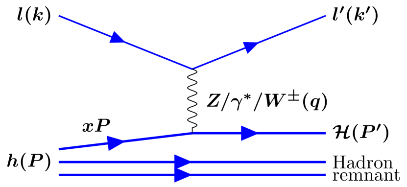
Figure 1: Schematic representation of Deep Inelastic Scattering process at Born level.

In this paper, we will only consider the neutral current electron scattering off a proton in a collider experiment. In this reaction, the final state lepton is a charged particle (electron or positron) that can be easily registered and identified in the detector.

With a fixed centre-of-mass energy, $\sqrt{s}=\sqrt{(k+P)^{2}}$, two independent, Lorentz-invariant, scalar quantities are sufficient to describe the deep inelastic scattering event kinematics in the Born approximation. Typically, the used quantities are:

• the negative squared four-momentum of the exchanged electroweak gauge boson:

  $$Q^{2}=-q\cdot q=-(k-k^{\prime})^{2},$$ (2)

• the Bjorken scaling variable, interpreted in the frame of a fast moving nucleon as the fraction of incoming nucleon longitudinal momentum carried by the struck parton:

  $$x=\frac{Q^{2}}{2P\cdot q}.$$ (3)

In addition to that, the inelasticity $y$ is used to define the kinematic region of interest. It is defined as the fraction of incoming electron energy taken by the exchanged boson in the proton rest frame

$$y=\frac{P\cdot q}{P\cdot k}.$$ (4)

Therefore, for the DIS an equation

$$Q^{2}=syx$$ (5)

holds. However, the Born-level picture of the DIS process is not sufficient for the description of the observed physics phenomena. A realistic description of DIS requires the inclusion of higher order QED and QCD processes Kwiatkowski:1990es .

2.2 Higher order corrections to deep-inelastic scattering process

The DIS process with leading order QED corrections can be written as

$$l(k)+h(P)\to l^{\prime}(k^{\prime})+\gamma(P_{\gamma})+X(P^{\prime})+{\rm remnant},$$ (6)

so the kinematics is defined not only by the kinematic of the scattered electron and the struck parton, but also by the momentum of the radiated photon, $P_{\gamma}$. The lowest order electroweak radiative corrections can be depicted in a form of Feynman diagrams as shown in Fig. 2 a)-d) and should be considered together with the virtual corrections e)-g).

(a)

(b)

(c)

(d)

(e)

(f)

(g)

(h)

(i)

(j)

(k)

Figure 2: Feynman diagrams for Deep Inelastic Scattering process with some leading order electroweak corrections a)-g) and QCD corrections h)-k). The proton remnant is omitted.

The Fig. 2 a),d) correspond to the initial state radiation (ISR) and the Fig. 2 b),c) to the final state radiation (FSR).

With the virtual corrections taken into account in the DIS process, Eq. 2 no longer holds, i.e.

$$q\cdot q\neq-(k-k^{\prime})^{2}.$$ (7)

The presence of higher order QCD processes, (e.g.  the boson-gluon fusion in Fig. 2 h) and QCD Compton Fig. 2 i),j)) makes the kinematic description of the DIS process even more complicated. Therefore, the exact definitions of the kinematic observables used in the analysis of the DIS events and the corresponding simulations are essential for the correct physics interpretation.

2.3 The simulation of the DIS events and the kinematic variables in the simulated events

The simulation of the inclusive DIS events in the Monte Carlo event generators (MCEGs) starts from the simulation at the parton level, i.e.  the simulation of the hard scattering process and the kinematics of the involved partons, e.g.  given by parton distribution functions (PDFs) Altarelli:1977zs for the given hadron and considering processes with all types of partons in the initial state. The modelling of the hard scattering process combines the calculations of the perturbative QED and/or QCD matrix elements for the $2\rightarrow n$ processes at parton level with the different QCD parton cascade algorithms designed to take into account at least some parts of the higher order perturbative QCD corrections not present in the calculations of matrix elements.

The simulated collision events on the particle (hadron) level are obtained using the parton level simulations as input and applying phenomenological hadronisation and particle decay models to them.

As of 2022, multiple MCEG programs are capable of simulating the inclusive DIS process at the hadron level with different levels of theory precision and sophistication of modelling of hadronisation, beam remnant and parton cascades, e.g. Pythia6 Sjostrand:2006za , Pythia8 Sjostrand:2014zea , SHERPA-MC Bothmann:2019yzt , WHIZARD Kilian:2007gr and Herwig7 Bellm:2015jjp . In addition to that, the Lepto Ingelman:1996mq , Ariadne Lonnblad:1992tz , Cascade Jung:2010si and Rapgap Jung:1993gf programs can simulate the DIS process using parts of the Pythia6 framework for the simulation of hadronisation processes and decays of particles.

As it was discussed above, DIS beyond the Born approximation has a complicated structure which involves QCD and QED corrections AbdulKhalek:2021gbh . The most recent MCEG programs, e.g.  Herwig7, Pythia8, SHERPA-MC, or WHIZARD, contain these corrections as a particular case of their own general-purpose frameworks or are able to use specialised packages like OpenLoops Cascioli:2011va , blackhat Bern:2013pya or MadGraph Alwall:2011uj . In general, the modern MCEGs do not specify their definitions of the DIS kinematic observables, but in some cases they can be calculated from the kinematics of the initial and final state, both for the true and reconstructed kinematics. For instance, under some assumptions, the $Q^{2}$ in the event could be calculated according to Eq. 2. The total elimination of the ambiguities for such calculations is not possible, as the final state kinematics even at the parton level depend on the kinematics of all the emitted partons. The calculations of the kinematic observables from the momenta of particles at hadron level add an additional ambiguity related to the identification of the scattered lepton and the distinction of that lepton from the leptons produced in the hadronisation and decay processes.

Contrary to the approaches adopted in modern MCEG programs, the MCEGs used for the HERA experiments relied upon generator-by-generator implementations of the higher order QED and QCD corrections specific for DIS or alternatively applied HERACLES Kwiatkowski:1990es for the corrections.

The way to get a simulation of the DIS collision even in a specific detector is the same as for any other type of particle collision event. It involves simulation of the particle transport through the detector material, simulation of detector response and is typically performed in Geant Brun:1987ma ; Agostinelli:2002hh or similar tools. The simulated detector response is passed to the experiment-specific reconstruction programs and should be indistinguishable from the real data recorded by the detector and processed in the same way.

2.4 Reconstruction of the kinematic variables at the detector level

The kinematics of the DIS events are reconstructed in collider experiments by identifying and measuring the momentum of the scattered lepton $l^{\prime}$ and/or the measurements of the hadronic final state ($\mathcal{H}$). The identification of the scattered lepton is ambiguous even at the particle level of the simulated DIS collision events. The same ambiguity is present in the reconstructed real and simulated data at the detector level. Therefore, the identification of the scattered electron candidate for the purposes of physics analyses is a complicated task on itself and was a subject of multiple studies in the past, some of which also involved neural network-related techniques Abramowicz:1995zi . In our paper, we rely on the standard method of the electron identification at the ZEUS experiment Abramowicz:1995zi and discuss solely the reconstruction of the kinematic variables using the identified electron and other quantities measured in the detector.

The physics analyses performed in the experiments at HERA relied on the following quantities for the calculation of the kinematic observables $x$ and $Q^{2}$:

• The energy ($E_{l^{\prime}}$) and polar angle ($\theta_{l^{\prime}}$) of the scattered electron. Most of the DIS experiments are equipped to register the scattered electron using the tracking and calorimeter detector subsystems. While the tracking system is able to provide information on the momentum of the scattered electron, the calorimeter system can be used to estimate the energy of the electron and the total energy of the collinear radiation emitted by the electron. At the detector level, the estimation of these energies can be done by comparing the momentum of the electron reconstructed in the tracking system and the energy deposits registered in the calorimeter system around the extrapolated path of the electron in the calorimeter.

• The energy of the HFS expressed in terms of the following convenient variables:

  $$\delta_{\mathcal{H}}=\sum_{i\in\mathcal{H}}E_{i}-P_{Z,i}$$ (8)

  and

  $$P_{T,\mathcal{H}}=\sqrt{\left(\sum_{i\in\mathcal{H}}P_{X,i}\right)+\left(\sum_{i\in\mathcal{H}}P_{Y,i}\right)},$$ (9)

where the sums run over the registered objects $i$ excluding the scattered electron. Depending on the analysis requirements, the used objects could be either registered tracks, energy deposits in the calorimeter system, or a combination of both.

The measurements of the quantities listed above overconstrain the reconstruction of the DIS kinematics. Therefore, in the simplest case, any subset of two observables in $E_{l^{\prime}}$, $\theta_{l^{\prime}}$, $\delta_{\mathcal{H}}$, and $P_{T,\mathcal{H}}$, can be used for the reconstruction.

In our analysis, we consider three specific classical reconstruction methods based on these observables which were used by the ZEUS collaboration in the past: the electron, the Jacques-Blondel, and the double-angle methods. We briefly provide some details on the methods in this section, while a more detailed description can be found elsewhere Bentvelsen:1992fu .

The electron (EL) method uses only measurements of the scattered lepton, $E_{l^{\prime}}$ and $\theta_{l^{\prime}}$, to do the reconstruction of $Q^{2}$ and $x$. The kinematic variables calculated from these measurements are given by:

$$Q^{2}_{EL}=2E_{l}E_{l^{\prime}}(1+\cos\theta_{l^{\prime}})$$ (10)

and

$$x_{EL}=\frac{E_{l}E_{l^{\prime}}(1+\cos\theta_{l^{\prime}})}{E_{P}(2E_{l}-E_{l^{\prime}}(1-\cos\theta_{l^{\prime}}))}.$$ (11)

The electron method provides precise reconstruction of kinematics, but, since it uses only information from the scattered lepton, this method is affected by initial and final state QED radiation. Namely, the QED radiation registered in the detector separately from the scattered electron will not be taken into account in the calculations with this method. Practically, the reconstruction with this method gives reasonable results when $E_{l}$ and $E_{l^{\prime}}$ are significantly different from one another, but the resolution and stability becomes poor otherwise.

The Jacques-Blondel (JB) method uses only measurements of the final state hadronic system, $\delta_{\mathcal{H}}$ and $P_{T,\mathcal{H}}$, for the reconstruction. The kinematic variables are calculated from these by:

$$Q^{2}_{JB}=\frac{2E_{l}P_{T,\mathcal{H}}^{2}}{2E_{l}-\delta_{\mathcal{H}}},$$ (12)

$$x_{JB}=\frac{2E_{l}Q^{2}_{JB}}{s\delta_{\mathcal{H}}}.$$ (13)

The JB method is resistant to possible biases because of unaccounted QED FSR, but requires precise measurements of the particles momenta in the hadronic final state. The factors that limit the precision of the measurements are the uncertainties in the particle identification, the finite resolution of the calorimeter and tracking detectors, the inefficiencies of these detectors, the impossibility of the particle detection around the beampipe, and the presence of objects that avoid detection (e.g.  neutrinos from particle decays).

The double-angle (DA) method combines measurements from the scattered lepton and the final-state hadronic system, $\theta_{l^{\prime}}$ and $\gamma_{\mathcal{H}}$, to perform the kinematic reconstruction as follows:

$$Q^{2}_{DA}=\frac{4E_{l}^{2}\sin\gamma_{\mathcal{H}}(1+\cos\theta_{l^{\prime}})}{\sin\gamma_{\mathcal{H}}+\sin\theta_{l^{\prime}}-\sin(\gamma_{\mathcal{H}}+\theta_{l^{\prime}})},$$ (14)

$$x_{DA}=\frac{E_{l}\sin\gamma_{\mathcal{H}}(1+\cos\theta_{l^{\prime}})}{E_{P}\sin\theta_{l^{\prime}}(1-\cos\gamma_{\mathcal{H}})},$$ (15)

where the angle $\gamma_{\mathcal{H}}$ is defined as

$$\cos\gamma_{\mathcal{H}}=\frac{P_{T,\mathcal{H}}^{2}-\delta_{\mathcal{H}}^{2}}{P_{T,\mathcal{H}}^{2}+\delta_{\mathcal{H}}^{2}}.$$ (16)

The angle $\gamma_{\mathcal{H}}$ depends on the ratio of the measured quantities $\delta_{\mathcal{H}}$ and $P_{T,\mathcal{H}}$, and thus, uncertainties in the hadronic energy measurement tend to cancel, leading to good stability of the reconstructed kinematic variables. Similar to the electron method, when $E_{l}$ and $E_{l^{\prime}}$ are significantly different from one another, the double-angle method provides reliable results, but the resolution and stability are poor otherwise.

2.5 The methodology of measurements in the deep inelastic $ep$ collisions

The methodology of measurements at lepton-hadron colliders in general is similar to the methodologies used at $e^{+}e^{-}$ and hadron-hadron colliders. Briefly, in the most cases the quantity of interest is measured from the real data registered in the detector corrected for detector effects. The corrections are estimated by comparing the analysis at the detector level with the same analysis at particle level using detailed simulations of the collision events with the inclusion of higher order QED and QCD processes.

The main difference between the measurements at lepton-hadron colliders and elsewhere, is in the way the measurements involve collision kinematics. At $e^{+}e^{-}$ colliders, the initial kinematics of the interactions is given by the lepton energies that are known parameters of the accelerators. Therefore, it is straightforward for most of the measurements in the $e^{+}e^{-}$ experiments to estimate the centre-of-mass energy of the hard collision process. In hadron-hadron collider experiments, there is no way to measure the kinematic properties of the partons initiating the collision process, as the involved partons cannot be observed in a free state and most measurements in the hadron-hadron collisions are inclusive in the kinematics of the initial state. The DIS collisions at electron-proton colliders take a middle stance between these cases. The kinematic observables of the DIS process are measured on an event-by-event basis at the detector level using the methods described above.

In an experiment, the measurements of event kinematics is affected by various effects. For a proper comparison of the measurements of HFS, e.g. jet cross-sections or event shape observables to corresponding perturbative QCD (pQCD) predictions, the detector-level measurements are unfolded for detector effects while hadronisation correction factors are calculated using MCEGs or specialised programs and applied to the pQCD predictions Currie:2017tpe ; H1:2021wkz ; Arbuzov:1995id ; Liu:2021jfp . The prescription for calculation of those correction factors vary depending on the HFS quantities measured and the used definitions of the kinematic observables. Typically, at ZEUS and other experiments at HERA, after the unfolding of the detector effects, the measurements were also scaled by radiation correction factors to facilitate a comparison to theoretical calculations available at Born level in QED, see e.g. Ref. ZEUS:2010fxa . The factors were obtained from separate high-statistics MC simulations. This is a well-understood Monte Carlo approach and our deep learning technique can be used with it in exactly the same way as the classical methods, both for the experimental and the MC data. For future DIS measurements, e.g.  at the upcoming Electron-Ion Collider, it is expected that the effects of QED and QCD radiation can be treated in an unified formalism Liu:2021jfp , with the QED effects taken into account into a factorised approach. Our DNN-based reconstruction of DIS kinematics is compatible with such a factorised approach as well.

Therefore, in this analysis, we keep the calculation of correction factors for QED and hadronisation effects out of scope and limit the discussion to detector-level measurements. At particle-level in the MC generated events, we use a single definition of “true” kinematic observables that is based on the kinematics of the exchanged boson extracted from the MC event information.

Namely, we use the definitions of the true-level observables $Q^{2}_{\rm true}$ and $x_{\rm true}$ that follow the definitions implemented in ZEUS Common NTuples Malka:2012hg ; AndriiVerbytskyifortheZEUS:2016zup and were used in many ZEUS analyses. With these definitions the $Q^{2}_{\rm true}$ is calculated directly from the squared four-momentum of the exchange boson $q_{\rm boson}$,

$$Q^{2}_{\rm true}=-|q_{\rm boson}|^{2}.$$ (17)

The $x_{\rm true}$ is calculated according to the formula

$$x_{\rm true}=\frac{Q^{2}_{\rm true}}{y_{\rm after\ ISR}s_{\rm after\ ISR}},$$ (18)

with

$$y_{\rm after\ ISR}=\frac{q_{\rm boson}\cdot P_{\rm proton\ beam}}{(P_{\rm lepton\ beam}-P_{\rm ISR\ radiation})\cdot P_{\rm proton\ beam}}$$ (19)

and

$$s_{\rm after\ ISR}=|P_{\rm proton\ beam}+P_{\rm lepton\ beam}-P_{\rm ISR\ radiation}|^{2},$$ (20)

where $P_{\rm proton\ beam}$, $P_{\rm lepton\ beam}$ and $P_{\rm ISR\ radiation}$ represent the four-momenta of the proton beam particles, lepton beam particles and the momenta lost by the lepton beam particles to ISR. Thus, $y_{\rm after\ ISR}$ corresponds to the fraction of energy of the bare lepton (i.e. without the ISR) transferred to the HFS in the centre of mass of the proton and $s_{\rm after\ ISR}$ to the centre-of-mass-energy squared of the proton and the incoming bare electron.

3 Machine learning methods

The reconstruction of DIS event kinematics is overconstrained by the previously mentioned measurements, $E_{l^{\prime}}$, $\theta_{l^{\prime}}$, $\delta_{\mathcal{H}}$, and $P_{T,\mathcal{H}}$. We trained an ensemble of deep neural networks (DNNs) to reconstruct $x$ and $Q^{2}$ by correcting results from classical reconstruction methods using the information on the scattered lepton and the final-state hadronic system.

The ensemble DNN method presented here is a new approach designed specifically to address this reconstruction problem. The remainder of this section discusses in detail specifics of the DNN architectures, the specific optimisation methods used to find the optimal parameters defining the DNNs, and the specific structure of the ensemble models. Shown rigorously in what follows, the main motivation for using the unique model is:

• the universal approximation capabilities of the DNN models with our specific architectures

• the necessary reduction in the approximation error with the increase in the depth of our DNN models

• avoidance of a degradation problem He:2015wrn in training due to the residual structure of our DNN models.

Further details on the DNN-based reconstruction method will be provided in Ref. Farhat:2022 .

3.1 Neural networks architecture

The problem of reconstruction of DIS event kinematics can be posed as a task to construct a functional relationship between a set of input variables ${\rm x}$ and a set of response variables ${\rm y}$. In many cases, such a relation is a continuous function, and can be approximated to arbitrary accuracy with a neural network. The corresponding neural network can have various architectures. The simplest architecture is a sequence of fully-connected, feed-forward (hidden) layers. For an input ${\rm x}\in\mathbb{R}^{m}$, the output of the first hidden layer is:

$$h^{1}({\rm x})=\alpha\left(A_{0}{\rm x}\right),\quad h^{1}\in\mathbb{R}^{d_{1}},$$ (21)

where $A_{0}:\mathbb{R}^{m}\to\mathbb{R}^{d_{1}}$ is an affine transformation, the composition of a translation and a linear mapping, and $\alpha:\mathbb{R}\to\mathbb{R}$ is a nonlinear function, called an activation function. Define the application of $\alpha$ on a vector ${\rm x}:=\left({\rm x}_{1},{\rm x}_{2},...,{\rm x}_{m}\right)^{T}\in\mathbb{R}^{m}$, by $\alpha({\rm x}):=\left(\alpha({\rm x}_{1}),\alpha({\rm x}_{2}),...,\alpha({\rm x}_{m})\right)^{T}$.

For $A_{1}:\mathbb{R}^{d_{1}}\to\mathbb{R}^{d_{2}}$, the output $h^{1}$ is passed into a second hidden layer:

$$h^{2}({\rm x})=\alpha\left(A_{1}h^{1}({\rm x})\right),\quad h^{2}\in\mathbb{R}^{d_{2}},$$ (22)

and so on, for a desired number of hidden layers. An affine transformation on the output of the final hidden layer is the output of the network. For $i\in\mathbb{N}$, call $d_{i}$ the number of nodes in hidden layer $i$.

Define $\mathbf{\Psi}^{D}_{m,n}(\alpha)$ to be the set of neural networks with $D$ hidden layers that map $\mathbb{R}^{m}\to\mathbb{R}^{n}$ with continuous, nonlinear activation function $\alpha$. If $\psi\in\mathbf{\Psi}^{D}_{m,n}$, then there exists a set of natural numbers $\{d_{i}\}_{i=0}^{D+1}\subset\mathbb{N}$ with $d_{0}=m$ and $d_{D+1}=n$, a set affine transformations $\{A_{i}:\mathbb{R}^{d_{i}}\to\mathbb{R}^{d_{i+1}}\}_{i=0}^{D}$, such that, for ${\rm x}\in\mathbb{R}^{m}$,

$$\begin{cases}h^{0}({\rm x})={\rm x},\\ h^{i+1}({\rm x})=\alpha\left(A_{i}h^{i}({\rm x})\right)\text{ for }0\leq i<D,\\ \psi({\rm x})=A_{D}h^{D}({\rm x}).\end{cases}$$ (23)

Specific universality properties of $\mathbf{\Psi}^{D}_{m,n}(\alpha)$ are proven in Refs. Hornik:1989 ; Leshno:1993 . In particular, there exists some element in the class of neural networks that is arbitrarily close to any continuous function. For this reason, we say that $\mathbf{\Psi}^{D}_{m,n}(\alpha)$ is dense in the space of continuous functions.

We consider a particular subclass of neural networks that also maintain the universal approximation property. We call it $\mathbf{\Phi}^{D}_{m,n}(\alpha)$. If a function $\phi\in\mathbf{\Phi}^{D}_{m,n}(\alpha)$, there exists a set of natural numbers $\{d_{i}\}_{i=0}^{D+1}\subset\mathbb{N}$ with $d_{0}=m$ and $d_{D+1}=n$, a set of affine transformations $\{A_{i}:\mathbb{R}^{d_{i}}\to\mathbb{R}^{d_{i+1}}\}_{i=0}^{D-1}$, a set of matrices $\{W_{i}\in\mathbb{R}^{d_{i}\times n}\}_{i=0}^{D}$, such that, for ${\rm x}\in\mathbb{R}^{m}$,

$$\begin{cases}h^{1}({\rm x})=\alpha\left(A_{0}{\rm x}\right),\\ h^{i+1}({\rm x})=\alpha\left(A_{i}h^{i}({\rm x})\right)\text{ for }0\leq i<D,\\ \phi({\rm x})=W_{0}{\rm x}+\sum_{i=1}^{D}W_{i}h^{i}({\rm x}).\end{cases}$$ (24)

Here the affine transformations $A_{i}$, $i=0,1,\dots,D-1$, have the form

$$A_{i}{\rm x}=M_{i}{\rm x}+{\rm b}_{i},\ \ \mbox{for}\ \ {\rm x}\in\mathbb{R}^{d_{i}}$$

for matrices $M_{i}\in R^{d_{i}\times d_{i+1}}$ and vectors ${\rm b}_{i}\in R^{d_{i+1}}$. The function $\phi$ defined by (24) is determined by matrices $M_{i}$ and $W_{i}$, and vectors ${\rm b}_{i}$ whose entries/components will be embraced in a single notation $\omega$ later. That is, $\phi=\phi_{\omega}$. When $\omega$ is chosen via an optimisation problem, $\phi({\rm x})$ is a function of the input variable ${\rm x}\in\mathbb{R}^{d_{0}}$.

Let $\mathbf{\Phi}^{D}_{m,n}(\alpha)$ be the function class in which we search for an optimal kinematic reconstruction method. In addition to the universality property, it can be shown that this class is good for searching for an appropriate reconstruction function because there the necessary reduction in the approximation error with the increase in the depth and the residual structure avoids a degradation problem in the weights during training Farhat:2022 .

3.2 Optimisation methods

In any given problem to be solved with the DNN, the task is to choose an optimal function from the class $\mathcal{F}=\mathbf{\Phi}^{D}_{m,n}(\alpha)$ to be a functional relationship between a set of input variables ${\rm x}$ and a set of response variables ${\rm y}$.

Each function $\phi\in\mathcal{F}$ is completely determined by the elements of the matrices and vectors that determine the values of the hidden layers. Let $\omega\in\mathbb{R}^{p}$ be the collection of all these elements, where $p$ is the total number of them. We can then write for any ${\rm x}\in\mathbb{R}^{m}$: $\phi({\rm x})=\phi_{\omega}({\rm x})$.

Choosing an optimal function from this class entails finding the collection of parameters $\omega$ in $\mathbb{R}^{p}$ that minimises $\mathcal{L}_{\mathcal{D}}$, the expected discrepancy or generalisation error between ${\rm y}$ and $\phi_{\omega}({\rm x})$, over the joint probability distribution of ${\rm x}$ and ${\rm y}$, $\mathcal{D}$, defined by:

$$\mathcal{L}_{\mathcal{D}}(\omega)=\mathop{\mathbb{E}}_{{\rm x},{\rm y}\sim\mathcal{D}}\ell(\omega,{\rm x},{\rm y})=\int\ell(\omega,{\rm x},{\rm y})d\mathcal{D}({\rm x},{\rm y}),$$ (25)

where $\ell$ is some loss function measuring the discrepancy between ${\rm y}$ and $\phi_{\omega}({\rm x})$.

With a randomly sampled data set $\{{\rm x}_{i},{\rm y}_{i}\}_{i=1}^{N}$, if $N$ is sufficiently large, then the generalisation error can be approximated by an empirical error:

$$\mathcal{L}_{\mathcal{D}}\approx\frac{1}{N}\sum_{i=1}^{N}\ell(\omega,{\rm x}_{i},{\rm y}_{i}).$$ (26)

This summation is sometimes called the fidelity term, as it measures the discrepancy between the data and model predictions. A commonly used fidelity term is the mean square error, with:

$$\ell(\omega,{\rm x}_{i},{\rm y}_{i})=\|{\rm y}_{i}-\phi_{\omega}({\rm x}_{i})\|^{2}_{2}.$$ (27)

The fidelity term used in this study is a modification of this, the mean square logarithmic error:

$$\ell(\omega,{\rm x}_{i},{\rm y}_{i})=\|\log({\rm y}_{i})-\log(\phi_{\omega}({\rm x}_{i}))\|^{2}_{2}.$$ (28)

Due to the universality of neural networks, there is a model that can achieve zero empirical error. However, in the presence of noise this means the model can overfit to the data sample and loose its generalisability. This problem can be addressed by adding a regularisation term to the optimisation problem as a penalty for certain irregular behaviour. Common regularisation terms include the $\ell^{2}$-norm, used to limit the size of the parameters, and the $\ell^{1}$-norm, which can induce sparse solutions. For out analysis, we choose the $\ell^{1}$-regularisation. The Theorem $1.3$ in Candes:2006 and Proposition 27 of Zhang:2009 provide an evidence that minimising the $\ell^{1}$ norm provides sparse optimal solutions with a minimal number of nonzero elements. Well-constructed models should be able to generalise the information from one given sample to any possible event. Thus, regularisation with the $\ell^{1}$ norm produces a model determined by a minimal number of parameters so that the optimal solution does not fit completely to the training set and loose its generalisability.

Therefore, the determination of the optimal neural network model consists of minimising this final loss function, the sum of the sample fidelity term and a weighted regularisation term:

$$\min_{\omega\in\mathbb{R}^{p}}\frac{1}{N}\sum_{i=1}^{N}\ell(\omega,{\rm x}_{i},{\rm y}_{i})+\mathcal{R}\cdot||\omega||_{1},$$ (29)

where $\ell$ is defined in Eq. 28 and $\mathcal{R}$ is a hyperparameter to determine the magnitude of the regularisation.

Expression 29 can be minimised using stochastic gradient methods on batches of the data sample Bertsekas:2000 . The training is accelerated using classical momentum methods Sutskever:2013 . In particular, randomly select an initial set of parameters $\omega^{0}$. Select a sequence of step sizes, or learning rates, ${\mathcal{L}}^{k}$ that diminish to zero. Randomly selecting a batch of data with indices $I\subset\{1,...,N\}$. Choosing a momentum parameter $\mu$. By defining:

$$v^{k+1}=\mu v^{k}-{\mathcal{L}}^{k}\nabla_{\omega}L_{I}(\omega^{k}),$$ (30)

$$\omega^{k+1}=\omega^{k}+v^{k+1}.$$ (31)

Then the sequence $\omega^{k}$ converges to a set of parameters defining the optimal neural network with the minimal generalisation error, in the sense described here.

3.3 The model

We construct a model to rigorously weight classically derived reconstructions of $x$ and $Q^{2}$ with corrections based on measurements from the final state lepton and hadronic system. The final reconstruction of these observables with the neural network approach are labelled below as $Q^{2}_{NN}$ and $x_{NN}$ respectively.

The constructed model is an ensemble of networks from the previously defined function class $\mathbf{\Phi}^{D}_{m,1}(\alpha)$, where $\alpha$ is the rectified linear unit (ReLU). The values of $D$ and $m$ vary with each network in the ensemble.

The NC DIS events studied in this analysis are by definition the events containing the scattered electron in the final state, therefore we aim to reconstruct the $Q^{2}_{NN}$ primarily from the related observables, i.e. using the properties of the electron directly measured in the experiment. In particular, we use as inputs three set of variables: the classically reconstructed kinematic observables
$\left(Q^{2}_{EL},Q^{2}_{DA},Q^{2}_{JB}\right)$, measurements on the scattered lepton $\left(E_{l^{\prime}},\theta_{l^{\prime}}\right)$, and measurements on the final-state hadronic system $\left(\delta_{\mathcal{H}},P_{T,\mathcal{H}}\right)$. We reconstruct the $Q^{2}$ in the form:

$$\begin{split}Q^{2}_{NN}&=A_{Q^{2}}\left(Q^{2}_{EL},Q^{2}_{DA},Q^{2}_{JB}\right)+L_{Q^{2}}\left(A_{Q^{2}},E_{l^{\prime}},\theta_{l^{\prime}}\right)+\\ &+H_{Q^{2}}\left(A_{Q^{2}},\delta_{\mathcal{H}},P_{T,\mathcal{H}}\right),\end{split}$$ (32)

in which $A_{Q^{2}}$ could be understood as a rigorous average of classically derived reconstructions, $L_{Q^{2}}$ is a correction term computed from the scattered lepton, and $H_{Q^{2}}$ is another correction term computed from the final-state hadronic system. In our analysis $A_{Q^{2}}$, $L_{Q^{2}}$, $H_{Q^{2}}$ are simultaneously trained networks in $\mathbf{\Phi}^{5}_{3,1}(\alpha)$, with each hidden layer of the networks containing 2000 nodes.

The $x$ observable for the NC DIS events is actually calculated from the electron-related observables as well. Therefore, we reconstruct $x_{NN}$, with $Q^{2}_{NN}$ also as an input, for a total of eight inputs ($x_{EL},x_{DA},x_{JB},E_{l^{\prime}},\theta_{l^{\prime}},\delta_{\mathcal{H}}$, $P_{T,\mathcal{H}},Q^{2}_{NN}$), in the form:

$$\begin{split}x_{NN}&=A_{x}\left(x_{EL},x_{DA},x_{JB}\right)+L_{x}\left(A_{x},Q^{2}_{NN},E_{l^{\prime}},\theta_{l^{\prime}}\right)+\\ &+H_{x}\left(A_{x},Q^{2}_{NN},\delta_{\mathcal{H}},P_{T,\mathcal{H}}\right),\end{split}$$ (33)

where $A_{x}$, $L_{x}$, and $H_{x}$ are defined similarly to $A_{Q^{2}}$, $L_{Q^{2}}$, and $H_{Q^{2}}$, but $A_{x}$ is a network in $\mathbf{\Phi}^{20}_{3,1}(\alpha)$ with each hidden layer containing 1000 nodes, and $L_{x}$, $H_{x}$ are networks in $\mathbf{\Phi}^{10}_{4,1}(\alpha)$, with each hidden layer containing 500 nodes.

The number of hidden layers and the number of nodes in each hidden layer were each progressively increased until sufficiently desirable results were achieved. Smaller networks provided good results on average, but larger networks were needed to find best results in small, specific regions of the kinematic space. A further increasing of the numbers of hidden layers and nodes per layer beyond the chosen values was found to not significantly alter the performance of the kinematic reconstruction, due to the convergence results of deep neural networks. The convergence theorems of deep neural networks with the ReLU activation function as the number of layers increases were recently established in xu2021 ; xu2021conv .

In the ensemble neural network model, we used the ReLU

$$\alpha({\rm x}):=\max({\rm x},0),\ \ {\rm x}\in\mathbb{R}$$ (34)

as the nonlinear activation function It has been shown Krizhevsky:2012 that with a gradient descent algorithm, using the ReLU function as the activation function provides a smaller training time compared to that with the use of functions with saturating nonlinearities, such as a sigmoid or hyperbolic tangent function. The reduced training time enabled us to experiment with more sophisticated networks. In addition to this, the ReLU functions do not need input normalisation to prevent them from saturating, which is a desirable property for the present analysis. Moreover, it was shown in xu2021 that the selection of the ReLU activation function produces a neural network as a piecewise linear function over a nonuniform partition, of the domain, determined by parameters involved in the affine transformations $A_{i}$. Such a structure ensures a good representability of the neural network and can overcome the problem of underfitting.

To accommodate for the large range of the $Q^{2}$ and $x$ variables in the analysis, we select the loss function defined in Eq. 28 for the training of the DNN models.

4 Experimental setup

The Monte Carlo simulated events used to train our deep neural networks were specifically generated using the conditions of $e^{\pm}p$ scattering in the ZEUS detector at HERA. A detailed description of the ZEUS detector can be found elsewhere ZEUS:1993aa .

In our analysis, we have used two samples of Monte Carlo simulated $e^{+}p$ DIS events that are provided by the ZEUS collaboration. These samples were generated with an inclusion of QED and higher order QCD radiative effects using the HERACLES 4.6.6 Kwiatkowski:1990es package with DJANGOH 1.6 Schuler:1991yg interface and the ARIADNE 4.12 and LEPTO 6.5.1 packages for the simulation of the parton cascade. For both samples the same set of kinematic cuts was applied during the generation, the same set of PDFs were used, CTEQ5D Lai:1999wy and the same hadronisation settings were used to model the hadronisation with the Pythia6 program. Therefore, the essential difference between the two samples is the way the higher order corrections are partially modelled with the corresponding algorithms (QCD cascades). Namely, the LEPTO MCEG utilises the parton shower approach Bengtsson:1987rw , while ARIADNE implements a color-dipole model Gustafson:1987rq . Accordingly, we label the data-sets produced by the LEPTO generator as “CDM” data sets and those with ARIADNE as “MEPS” data sets.

The generated particle-level events were passed through the ZEUS detector and trigger simulation programs based on Geant 3.21 Brun:1987ma , assuming the running conditions of the ZEUS experiment in the year 2007 with a proton beam energy of 920 GeV. The simulated detector response was processed and reconstructed using exactly the same software chain and the same procedures as being used for real data. The results of the processing were saved in ROOT Antcheva:2011zz files in a form of ZEUS Common NTuples Malka:2012hg ; AndriiVerbytskyifortheZEUS:2016zup , a format that can be easily used for physics analysis without any ZEUS-specific software.

5 Event selection

The selection of events for the neural network training is motivated by the selection procedure applied in the previous ZEUS analyses Breitweg:1999id ; Chekanov:2006yc ; Chekanov:2006hv ; Chekanov:2006xr ; Abramowicz:2010ke ; Abramowicz:2010cka . Even though the presented analysis performed on the Monte Carlo simulated events, the selection cuts are choosen and applied as if the analysis is performed on real data for the purpose of being as close as possible to the measurements. The general motivation for these cuts is the same as in many analyses performed by the ZEUS collaboration: to define unambiguously the phase space of the measurement, ensure low fraction of background events, and a reasonable description of the detector acceptance by Monte Carlo simulations.

5.1 Phase space selection

The phase space for the training of the neural networks in this analysis is selected as $100{\,\text{Ge}\kern-0.66666pt\text{V\/}}^{2}<Q^{2}<20480{\,\text{Ge}\kern-0.66666pt\text{V\/}}^{2}$, being close to the phase space of the physics analysis in Ref. Abramowicz:2010ke .

In the phase-space region at low $x$ and very low inelasticity $y$, the QED predictions from the Monte Carlo simulations are not reliable because of a limit of higher orders in the calculations Lontkovskyi:2015 . To avoid these phase-space regions, the events are required to have $y_{JB}\cdot(1-x_{DA})^{2}>0.004$ and $y_{JB}>0.04$ Lontkovskyi:2015 . To ensure optimal electron identification and electron energy resolution, similar to the previous physics analyses, a kinematic cut $0.2<y_{EL}<0.7$ is used.

5.2 Event selection

The deep inelastic scattering events of interest are those characterised by the presence of a scattered electron in the final state and a significant deposit of energy in the calorimeter from the hadronic final state. The scattered electrons are registered in the detector as localised energy depositions primarily in the electromagnetic part of the calorimeter, with little energy flow into the hadronic part of the calorimeter. On the other hand, hadronic showers propagate in the detector much more extensively, both transversely and longitudinally.

In addition to the DIS process, there are also background processes which leave similar signatures in the detector as those described above. Therefore, the correct and efficient identification of the scattered lepton is crucial for the selection of the NC DIS events. For this analysis, the SINISTRA algorithm is used to identify lepton candidates Abramowicz:1995zi . Based on the information from the detector and the results of the SINISTRA algorithm, the following selection criteria are applied to select the events for the further analysis:

• Detector status: It is required that for all the events the detector was fully functional.

• Electron energy: At least one electron candidate with energy greater than $10{\,\text{Ge}\kern-0.66666pt\text{V\/}}$ Abramowicz:2010ke is identified in the event.

• Electron identification probability: The SINISTRA Abramowicz:1995zi probability of a lepton candidate being the DIS lepton was required to be greater than 90%. If several lepton candidates satisfy this condition, the candidate with the highest probability is used. In addition to this, there must be no problems reported by the SINISTRA algorithm.

• Electron isolation: To assist in removing events where the energy deposits from the hadron system overlap with those of the scattered lepton, the fraction of the energy not associated to the lepton is required to be less than 10% over the total energy deposited within a cone around the lepton candidate. The cone is defined with a radius of $0.7$ units in the pseudorapidity-azimuth plane around the lepton momentum direction Abramowicz:2010ke .

• Electron track matching: The tracking system covers the region of polar angles restricted to $0.3<\theta<2.85$ rad. Electromagnetic clusters within that region that have no matching track are most likely photons. If the lepton candidate is within this region, the presence of a matched track is required. This track must have a distance of closest approach between the track extrapolation point at the front surface of the CAL and the cluster centre-of-gravity-position of less than 10 cm. The track energy must be greater than 3 GeV Abramowicz:2010ke .

• Electron position: To minimise the impact of imperfect simulation of some detector regions, additional requirements on the position of the electromagnetic shower are imposed. The events in which the lepton is found in the following regions ($x$,$y$ and $z$ being the cartesian coordinates in the ZEUS detector) are rejected Perrey:2011hga :

  • $\sqrt{x^{2}+y^{2}}<18\text{ cm}$, regions close the beam pipe

  • $z<-148\text{ cm}$ and $y>90\text{ cm}$ and $-14<x<12\text{ cm}$, a part of the RCAL where the depth was reduced due to the cooling pipe for the solenoid (chimney),

  • $-104<z<-98.5\text{ cm}$ or $164<z<174\text{ cm}$, regions in-between calorimeter sections (super-crack).

• Primary vertex position: It was required that the reconstructed primary vertex position is close to the central region of the detector, applying the selection $-28.5<Z_{\rm vtx}<26.7\text{ cm}$ Abramowicz:2010ke .

• Energy-longitudinal momentum balance: To suppress photoproduction and beam-gas interaction background events and imperfect Monte Carlo simulations of those, restrictions are put on the energy-longitudinal momentum balance. This quantity is defined as:

  $$\delta=\delta_{l}+\delta_{\mathcal{H}}=(E_{l^{\prime}}-P_{z,l^{\prime}})+(E_{\mathcal{H}}-P_{z,\mathcal{H}})=\sum_{i}(E_{i}-P_{z,i}),$$ (35)

  where the final summation index runs over all energy deposits in the detector. In this analysis, we apply a condition of $38<\delta<65{\,\text{Ge}\kern-0.66666pt\text{V\/}}$ Abramowicz:2010ke .

• Missing transverse energy: To remove beam-related background and cosmic-ray events, a cut on the missing energy is imposed. $P_{T,\rm miss}/\sqrt{E_{T}}<2.5{\,\text{Ge}\kern-0.66666pt\text{V\/}}^{1/2}$, where $E_{T}$ is the total transverse energy in the CAL and $P_{T,\rm miss}$ is the missing transverse momentum, the transverse component of the vector sum of the hadronic final state and scattered electron momenta.

6 Training the DNN models

We use the neural network models defined in Sec. 3.3 and consider them as optimisation problem in terms of Eq. 29, i.e., we minimise the loss function across the selected training set and satisfy sparse regularity conditions. Every neural network making the ensemble model for $x$ and $Q^{2}$ are trained simultaneously. The optimal regularity condition depends on the selection of the training set, the events batch size, the initial learning rate, and the regularisation parameter. We aim to select these in a way that minimises overfitting in particular regions of the kinematic space while still maximising the mean accuracy of the model.

We select a set of events from the “MEPS” data sets for training, as described in Sec. 5, and define the true values of the $x$ and $Q^{2}$ as described in Sec. 2.3. Fig. 3 shows a distribution of selected events in the $(x_{\rm true},Q^{2}_{\rm true})$ plane and the boundaries of the chosen analysis bins.

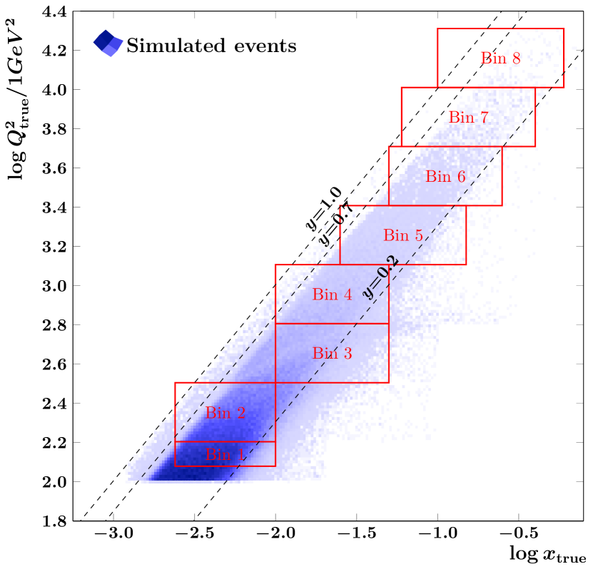
Figure 3: Distribution of events from the training set in $(x_{\rm true},Q^{2}_{\rm true})$ plane and the boundaries of the analysis bins from Tab. 3.

First, we train the network to reconstruct $Q^{2}$ by optimising Eq. 29 with an initial learning rate of $\mathcal{L}=1.0\times 10^{-5}$ and a regularisation parameter of ${\mathcal{R}=1.0\times 10^{-5}}$. We select a batch size of 10000.

The reconstruction of $x$ is more complex. We fix the regularisation parameter to $\mathcal{R}=1.0\times 10^{-5}$ and select optimal parameters for the learning rate ${\mathcal{L}}$ and batch size ${\mathcal{B}}$ experimentally by varying the learning rate against the batch size. The appropriate selection of these parameters ensures fast convergence of the stochastic gradient method by balancing noise in the gradients with the stability of the algorithm. For each set of parameters, ten attempts are made and the best result in terms of the mean square error of the $x$ reconstruction model over the training set is chosen. The results are listed in Tab. 6. The smaller learning rate assures a higher stability of the results than a larger learning rate. It prolongs the training process but avoids a poor convergence of the learning process as observed for larger learning rates. The larger batch size does not offer any advantages in our analysis as shown in Tab. 6. We, therefore, select an initial learning rate of $10^{-5}$ with a minimal batch size.

	RMS of $\log{x}-\log{x_{\rm true}}$
${\mathcal{L}}$	${\mathcal{B}}$	${\mathcal{B}}$	${\mathcal{B}}$
	10000	50000	100000
$1.0\times 10^{-7}$	0.1507	0.1523	0.1598
$5.0\times 10^{-7}$	0.1568	0.1575	0.1575
$1.0\times 10^{-6}$	0.1504	0.1585	0.1547
$5.0\times 10^{-6}$	0.2384	0.2284	0.1829
$1.0\times 10^{-5}$	0.2182	2.5972	2.2767
$1.5\times 10^{-5}$	0.2122	1.7751	1.6028
$2.0\times 10^{-5}$	3.0258	0.2607	0.2852
$5.0\times 10^{-5}$	3.6962	2.4858

Table 1: Resolution of $\log{x}$ reconstruction after 200 epochs of training with different values of initial learning rate ${\mathcal{L}}$ and batch size ${\mathcal{B}}$.

To choose the regularisation parameter close to the optimal one, we vary its value with constant batch size of $10000$ and initial learning rate of $10^{-5}$ and again observe the mean square error of the $x$ reconstruction model over the training set. For each set of parameters, ten attempts are made and the best result is chosen. The results are presented in Tab. 6. Accordingly, we choose a regularisation parameter of $10^{-6}$. Using this regularisation, the neural network models for both $x$ and $Q^{2}$ are defined by weight parameters, of which 50% are effectively zero, or less than $10^{-8}$

${\mathcal{R}}$	RMS of $\log{x}-\log{x_{\rm true}}$
$1.0\times 10^{-6}$	0.1493
$1.0\times 10^{-5}$	0.1494
$1.0\times 10^{-4}$

Table 2: Resolution of $\log{x}$ reconstruction after 200 epochs of training with different values of regularisation parameter ${\mathcal{R}}$.

Following the suggestions in Ref. Smith:2017 , we start with a small batch size, and increase it in initial training epochs. We test this approach by comparing the mean square error of the $x$ reconstruction model over the training set over the first 200 epochs of training over three different training regimes. The results are summarised in Fig. 4 and imply to use a gradually increasing batch size up to a maximum batch size of $1000$.

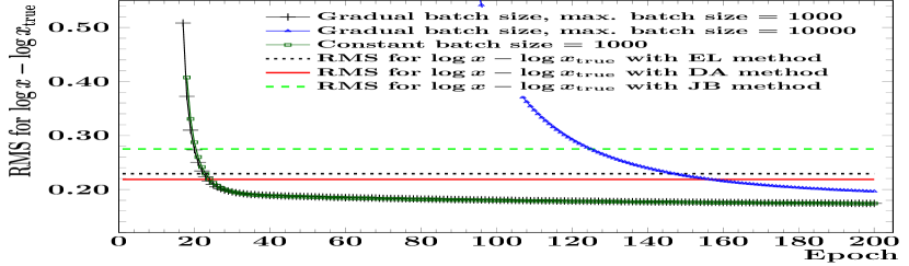
Figure 4: Training history for $x$ reconstruction model using different training parameters but the same $Q^{2}$ reconstruction model obtained with ${\mathcal{L}}=1.0\times 10^{-5}$, ${\mathcal{R}}=1.0\times 10^{-6}$ and ${\mathcal{B}}=10000$. In each of the cases, the initial learning rate was set to ${\mathcal{L}}=1.0\times 10^{-5}$ and the regularisation parameter to ${\mathcal{R}}=1.0\times 10^{-6}$.

7 Results

We evaluate the performance of our approach for the reconstruction of DIS kinematics by applying it to detailed Monte Carlo simulations from the ZEUS experiment and by comparing our results to the results from the electron, double-angle, and Jacques-Blondel reconstruction methods. For the comparison, we use various combinations of statistically independent data sets, one for the training, and another for the evaluation. In our systematic studies, we have found no signs of overtraining and also no indication that the results depend on the selected Monte Carlo simulations. For the results presented in this section, we use the “MEPS” data set for the training and the “CDM” data set for evaluation. The main quantities of the comparison are the resolutions of the reconstructed variables $\log{Q^{2}/1{\,\text{Ge}\kern-0.66666pt\text{V\/}}^{2}}$ and $\log{x}$ as measured in selected $x-Q^{2}$ regions (bins). The resolutions are defined as $\sqrt{\sum^{N}_{i}\left(\log{Q^{2}_{i}/1{\,\text{Ge}\kern-0.66666pt\text{V\/}}^{2}}-\log{Q^{2}_{i,\rm true}/1{\,\text{Ge}\kern-0.66666pt\text{V\/}}^{2}}\right)^{2}/N}$ and $\sqrt{\sum^{N}_{i}\left(\log{x_{i}}-\log{x_{i,\rm true}}\right)^{2}/N}$, where $N$ stands for the number events in the corresponding bin. The boundaries of the bins are given in Tab. 3 and are chosen to be close to the bins used in ZEUS DIS analyses, e.g. in Ref. Chekanov:2006hv .

Bin	$Q^{2}$ (${\,\text{Ge}\kern-0.66666pt\text{V\/}}^{2}$)	$x$
1	120 - 160	0.0024 - 0.010
2	160 - 320	0.0024 - 0.010
3	320 - 640	0.01 - 0.05
4	640 - 1280	0.01 - 0.05
5	1280 - 2560	0.025 - 0.150
6	2560 - 5120	0.05 - 0.25
7	5120 - 10240	0.06 - 0.40
8	10240 - 20480	0.10 - 0.60

Table 3: Kinematic bins in $x$ and $Q^{2}$, see also Fig. 3.

The distributions of the $\log{Q^{2}/1{\,\text{Ge}\kern-0.66666pt\text{V\/}}^{2}}-\log{Q^{2}_{\rm true}/1{\,\text{Ge}\kern-0.66666pt\text{V\/}}^{2}}$ and $\log{x}-\log{x_{\rm true}}$ quantities are given in the Fig. 6 and Fig. 6, respectively. The numerical values for the resolution are summarised for all the bins and methods in Tab. 6. The DNN optimisation procedure minimises the generalisation error described in Eq. 25 plus the regularisation penalty, so distributions in Figs. 6 and  6 do not necessarily peak at zero. In addition to that, Fig. 6 and Fig. 6 show the two dimensional distributions of events in $\log{Q^{2}/1{\,\text{Ge}\kern-0.66666pt\text{V\/}}^{2}}$ vs. $\log{Q^{2}_{\rm true}/1{\,\text{Ge}\kern-0.66666pt\text{V\/}}^{2}}$ and $\log{x}$ vs. $\log{x_{\rm true}}$ planes.

Figure 5: Distributions of $\log{Q^{2}/1{\,\text{Ge}\kern-0.59999pt\text{V\/}}^{2}}-\log{Q^{2}_{\rm true}/1{\,\text{Ge}\kern-0.59999pt\text{V\/}}^{2}}$ for various reconstruction methods in individual analysis bins. For better visibility, the data points for each reconstruction method are connected with straight lines.

The comparison of the DNN-based approach with the classical methods demonstrates that the DNN-based approach is well suited for the reconstruction of DIS kinematics. Specifically, for most of the bins, our approach provides the best resolution as measured by the standard deviation of the logarithmic differences of true and reconstructed variables. The better performance of the DNN-based approach in most of the bins is a consequence of using additional available information about the final state. In this respect, the DNN-based approach is similar to averaging of the values provided by the classical methods with some weights or to alternative approaches for the same task, e.g. see kinematic fitting in Ref. Aggarwal:2012 . However, in addition to a better resolution, the reconstruction with the DNN has an important advantage over the classical methods or any simple combination of them. It allows to combine the methods without the intrinsic biases of each method and enables an extension of the model with additional physics observables in a robust way.

Figure 6: Distributions of $\log{x}-\log{x_{\rm true}}$ for various reconstruction methods in individual analysis bins. For better visibility, the data points for each reconstruction method are connected with straight lines.

Table 4: Resolution of the reconstructed kinematic variables in bins of $x$ and $Q^{2}$. The resolution for $x$ and $Q^{2}$ is defined as the RMS of the distributions $\log(x)-\log(x_{\rm true})$ and $\log(Q^{2})-\log(Q^{2}_{\rm true})$ respectively.

Figure 7: Distribution of events in $L_{\rm reco}=\log{Q^{2}/1{\,\text{Ge}\kern-0.59999pt\text{V\/}}^{2}}$ versus $L_{\rm true}=\log{Q^{2}_{\rm true}/1{\,\text{Ge}\kern-0.59999pt\text{V\/}}^{2}}$ plane for different reconstruction methods in individual analysis bins.

Figure 8: Distribution of events in $L_{\rm reco}=\log{x}$ versus $L_{\rm true}=\log{x_{\rm true}}$ plane for different reconstruction methods in individual analysis bins.

The resolution is improved by the DNN-based approach in two ways. For the first couple of bins, the main improvement is caused by the more precise estimation of the reconstructed observables. This is clearly seen in Figs. 6 and 6. For the bins with higher $Q^{2}$ and $x$ the main improvement is due to the rejection of outliers, which can be seen in Figs. 6 and 6. The bins with higher $Q^{2}$ and $x$ also demonstrate another, very specific advantage on the DNN approach. Due to the low number of training events in the high $Q^{2}$ and $x$ region, it would not be possible to train a DNN model or combine the $Q^{2}$ and $x$ observables with other methods using information from this region only. However, the DNN training process benefits from the constraints from the higher number of events available elsewhere in the kinematical space and delivers models that perform well even in the bins with highest $Q^{2}$ and $x$.

8 Conclusions

We have presented the use of DNN to reconstruct the kinematic observables $Q^{2}$ and $x$ in the study of neutral current DIS events at the ZEUS experiment at HERA. The DNN models are specially designed to be effective in their universal approximation capability, robust in the sense that increasing the depth of the networks will necessarily reduce empirical error, and computationally efficient with a structure that avoids “vanishing” gradients arising in the backpropagation algorithm.

Compared to the classical reconstruction methods, the DNN-based approach enables significant improvements in the resolution of $Q^{2}$ and $x$. At the same time, it is evident that the usage of the DNN approach allows to match easily any definition of $Q^{2}$ and $x$ at the true level that is preferred for a given physics analysis.

The large samples of simulated data required for the training of the DNN can be generated rapidly at modern data centres. Also, DNN allow to effectively extract information from large data sets. This suggests that our new approach for the reconstruction of DIS kinematics can serve as a rigorous method to combine and outperform the classical reconstruction methods at ongoing or upcoming DIS experiments. We will extend the approach beyond inclusive DIS measurements and will study next the use of DNN for the reconstruction of event kinematics in semi-inclusive and exclusive DIS measurements.

Acknowledgement

We are grateful to the ZEUS Collaboration for allowing us to use ZEUS Monte Carlo simulated samples in this analysis and the Data Preservation efforts DPHEP:2015npg in DESY and Max-Planck for Physics that made this analysis possible. We thank R. Aggarwal, C. Fanelli, Y. Furletova, D. Higinbotham, D. Lawrence, S. Menke, A. Vossen, and R. Yoshida for helpful discussions.

The work of M. Diefenthaler was supported by the US Department of Energy, Office of Science, Office of Nuclear Physics contract DE-AC05-06OR23177, under which Jefferson Science Associates, LLC operates the Thomas Jefferson National Accelerator Facility.

A. Farhat and Y. Xu were supported in part by National Science Foundation under grant DMS-1912958. A. Farhat was also supported by an EIC Center Fellowship at the Thomas Jefferson National Accelerator Facility.

Appendix A Software used in the analysis

The ROOT package Antcheva:2011zz of version 6.22 was used to read the ZEUS data, provided by the data preservation at Max-Planck for Physics DPHEP:2015npg , analyze it and prepare plain text (or ROOT files) with selected information to be used with the ML tools. The selected information from the plain text (or ROOT) files was piped using the pandas package mckinney-proc-scipy-2010 into Keras chollet2015keras interface to tensorflow tensorflow2015whitepaper 2.3.0 library to train the ML models. The packages Eigen eigenweb , frugally-deep fdeep , JSON for Modern C++ nlohmann and FunctionalPlus fplus were used for execution of the trained models after these were converted into frugally-deep model format fdeep to be used with C++ application. The dependencies for the tensorflow were supplied from the PyPi repository. The training was performed using libraries for computing on GPUs from the CUDA cuda framework of version 10.1. We are grateful to MPCDF for the ability to compile and execute the codes on the HPC cluster “Cobra” in  cobra . The operation system used was Linux on ${\rm x}86\_64$ architecture using gcc Stallman:2009:UGC:1593499 of version 7.3 and python python3 of version 3.6.8.

The figures with the final results were produced with the PGFPlots pgfplots package. 10

B.H. Wiik et al., HERA - A Proposal for a Large Electron Proton Colliding Beam Facility at DESY. https://old.inspirehep.net/record/19436/files/Fulltext.pdf, 1981

DUNE Coll., B. Abi et al., Volume I. Introduction to DUNE. JINST 15, T08008 (2020). arXiv:2002.0296

F. Gautheron et al., COMPASS-II Proposal. https://cds.cern.ch/record/1265628/files/SPSC-P-340.pdf, 2010

Arrington, J. and others, Physics with CEBAF at 12 GeV and Future Opportunities.  (2021). arXiv:2112.0006

Aschenauer, E. C. and Thorne, R. S. and Yoshida, R., PDG Chapter 18: Structure Functions. PTEP, 2022, doi:10.1093/ptep/ptac097

G.A. Voss and B.H. Wiik, The Electron proton collider HERA. Ann. Rev. Nucl. Part. Sci. 44, 413 (1994)

H1 and ZEUS Colls., H. Abramowicz et al., Combination of measurements of inclusive deep inelastic ${e^{\pm}p}$ scattering cross sections and QCD analysis of HERA data. Eur. Phys. J. C75, 580 (2015). arXiv:1506.0604

U. Bassler and G. Bernardi, On the kinematic reconstruction of deep inelastic scattering at HERA: The Sigma method. Nucl. Instrum. Meth. A361, 197 (1995). arXiv:hep-ex/9412004

R. Abdul Khaleket et al., Science Requirements and Detector Concepts for the Electron-Ion Collider: EIC Yellow Report.  (2021). arXiv:2103.0541

U. Holm, The ZEUS detector: Status report 1993. http://dx.doi.org/10.3204/PUBDB-2017-12635, 1993

H. Abramowicz, A. Caldwell and R. Sinkus, Neural network based electron identification in the ZEUS calorimeter. Nucl. Instrum. Meth. A365, 508 (1995). arXiv:hep-ex/9505004

A. Accardi et al., Electron Ion Collider: The Next QCD Frontier. Eur. Phys. J. A52, 268 (2016). arXiv:1212.1701

Junze Liu et al., Deep-Learning-Based Kinematic Reconstruction for DUNE.  (2020). arXiv:2012.0618

H1, I. Abt et al., The H1 detector at HERA. Nucl. Instrum. Meth. A 386, 310 (1997)

A. Kwiatkowski, H. Spiesberger and H.J. Mohring, Heracles: An Event Generator for $ep$ Interactions at HERA Energies Including Radiative Processes: Version 1.0. Comput. Phys. Commun. 69, 155 (1992)

G. Altarelli and G. Parisi, Asymptotic Freedom in Parton Language. Nucl. Phys. B126, 298 (1977)

T. Sjöstrand, S. Mrenna and P.Z. Skands, PYTHIA 6.4 physics and manual. JHEP 05, 026 (2006). arXiv:hep-ph/0603175

T. Sjöstrand et al., An introduction to PYTHIA 8.2. Comput. Phys. Commun. 191, 159 (2015). arXiv:1410.3012

Sherpa Coll., E. Bothmann et al., Event generation with SHERPA 2.2. SciPost Phys. 7, 034 (2019). arXiv:1905.0912

W. Kilian, T. Ohl and J. Reuter, WHIZARD: Simulating Multi-Particle Processes at LHC and ILC. Eur. Phys. J. C71, 1742 (2011). arXiv:0708.4233

J. Bellm et al., Herwig 7.0/Herwig++ 3.0 release note. Eur. Phys. J. C76, 196 (2016). arXiv:1512.0117

G. Ingelman, A. Edin and J. Rathsman, LEPTO 6.5: A Monte Carlo generator for deep inelastic lepton - nucleon scattering. Comput. Phys. Commun. 101, 108 (1997). arXiv:hep-ph/9605286

L. Lönnblad, ARIADNE version 4: a program for simulation of QCD cascades implementing the color dipole model. Comput. Phys. Commun. 71, 15 (1992)

H.  Jung et al., The CCFM Monte Carlo generator CASCADE version 2.2.03. Eur. Phys. J. C70, 1237 (2010). arXiv:1008.0152

H. Jung, Hard diffractive scattering in high-energy $ep$ collisions and the Monte Carlo generator RAPGAP. Comput. Phys. Commun. 86, 147 (1995)

F. Cascioli, P. Maierhofer and S. Pozzorini, Scattering Amplitudes with OpenLoops. Phys. Rev. Lett. 108, 111601 (2012). arXiv:1111.5206

Z. Bern et al., The BlackHat library for one-loop amplitudes. J. Phys. Conf. Ser. 523, 012051 (2014). arXiv:1310.2808

J. Alwall et al., MadGraph 5 : Going Beyond. JHEP 06, 128 (2011). arXiv:1106.0522

R. Brun et al., GEANT3. https://cds.cern.ch/record/1119728/files/CERN-DD-EE-84-1.pdf, 1987

GEANT4 Coll., S. Agostinelli et al., GEANT4–a simulation toolkit. Nucl. Instrum. Meth. A506, 250 (2003)

S. Bentvelsen, J. Engelen and P. Kooijman, Reconstruction of $(x,Q^{2})$ and extraction of structure functions in neutral current scattering at HERA, Workshop on Physics at HERA Hamburg, Germany, October 29-30, 1991, pp. 23–42. (1992)

J. Currie et al, NNLO QCD corrections to jet production in deep inelastic scattering. JHEP 07, 018 (2017). arXiv:1703.0597. [Erratum: JHEP 12, 042 (2020)]

H1, Andreev, V. and others, Measurement of Lepton-Jet Correlation in Deep-Inelastic Scattering with the H1 Detector Using Machine Learning for Unfolding. Phys. Rev. Lett. 128, 132002 (2022). arXiv:2108.1237

A. Arbuzov el al., Hector 1.00: A Program for the calculation of QED, QCD and electroweak corrections to $ep$ and $lepton^{\pm}N$ deep inelastic neutral and charged current scattering. Comput. Phys. Commun. 94, 128 (1996). arXiv:hep-ph/9511434

T. Liu et al., A new approach to semi-inclusive deep-inelastic scattering with QED and QCD factorization. JHEP 11, 157 (2021). arXiv:2108.1337

ZEUS, H. Abramowicz et al., Inclusive-jet cross sections in NC DIS at HERA and a comparison of the kT, anti-kT and SIScone jet algorithms. Phys. Lett. B 691, 127 (2010). arXiv:1003.2923

ZEUS Coll., J. Malka and K. Wichmann, The ZEUS data preservation project. J. Phys. Conf. Ser. 396, 022033 (2012)

ZEUS Coll., A. Verbytskyi, The ZEUS long term data preservation project. PoS DIS2016, 264 (2016). arXiv:1607.0189

K. He et al., Deep Residual Learning for Image Recognition.  (2015). arXiv:1512.0338

A. Farhat, Deep multiscale learning and applications to nuclear physics, Ph.D. thesis, Old Dominion University, in preparation

K. Hornik, M. Stinchcombe and H. White, Multilayer feedforward networks are universal approximators. Neural Networks 2, 359 (1989)

M. Leshno, V.Y. Lin, A. Pinkus and S. Schocken, Multilayer feedforward networks with a nonpolynomial activation function can approximate any function. Neural Networks 6, 861 (1993)

E. Candes, J. Romberg and T. Tao, Robust Uncertainty Principles : Exact Signal Frequency Information. IEEE Transactions on Information Theory 52, 489 (2006)

H. Zhang, Y. Xu and J. Zhang, Reproducing kernel Banach spaces for machine learning. Journal of Machine Learning Research, p. 2741 (2009)

D.P. Bertsekas and J. Tsitsiklis, Gradient convergence in gradient methods with errors. SIAM Journal on Optimization 10, 627 (2000)

I. Sutskever et al., On the importance of initialization and momentum in deep learning. ICML’13: Proceedings of the 30th International Conference on International Conference on Machine Learning 28, 1139–1147 (2013)

Y. Xu and H. Zhang, Convergence of deep relu networks.  (2021). arXiv:2107.1253

Y. Xu and H. Zhang, Convergence of deep convolutional neural networks. Neural Networks 153, 553 (2022)

A. Krizhevsky et al., ImageNet Classification with Deep Convolutional Neural Networks, in Advances in Neural Information Processing Systems 25, eds. F. Pereira and C. J. C. Burges and L. Bottou and K. Q. Weinberger, pp. 1097–1105. Curran Associates, Inc., 2012

G.A. Schuler and H. Spiesberger, DJANGO: The Interface for the event generators HERACLES and LEPTO, Workshop on Physics at HERA. (1991)

CTEQ Coll., H.L. Lai et al., Global QCD analysis of parton structure of the nucleon: CTEQ5 parton distributions. Eur. Phys. J. C12, 375 (2000). arXiv:hep-ph/9903282

M. Bengtsson and T. Sjostrand, Parton Showers in Leptoproduction Events. Z. Phys. C37, 465 (1988)

G. Gustafson and U. Pettersson, Dipole Formulation of QCD Cascades. Nucl. Phys. B306, 746 (1988)

I. Antcheva et al., ROOT: A C++ framework for petabyte data storage, statistical analysis and visualization. Comput. Phys. Commun. 182, 1384 (2011)

ZEUS Coll., J. Breitweg et al., Measurement of high $Q^{2}$ neutral current $e^{+}p$ deep inelastic scattering cross-sections at HERA. Eur. Phys. J. C11, 427 (1999). arXiv:hep-ex/9905032

ZEUS Coll., S. Chekanov et al., Jet-radius dependence of inclusive-jet cross-sections in deep inelastic scattering at HERA. Phys. Lett. B649, 12 (2007). arXiv:hep-ex/0701039

ZEUS Coll., S. Chekanov et al., Event shapes in deep inelastic scattering at HERA. Nucl. Phys. B767, 1 (2007). arXiv:hep-ex/0604032

ZEUS Coll., S. Chekanov et al., Inclusive-jet and dijet cross-sections in deep inelastic scattering at HERA. Nucl. Phys. B765, 1 (2007). arXiv:hep-ex/0608048

ZEUS Coll., H. Abramowicz et al., Inclusive-jet cross sections in NC DIS at HERA and a comparison of the kT, anti-kT and SIScone jet algorithms. Phys. Lett. B691, 127 (2010). arXiv:1003.2923

ZEUS Coll., H. Abramowicz et al., Inclusive dijet cross sections in neutral current deep inelastic scattering at HERA. Eur. Phys. J. C70, 965 (2010). arXiv:1010.6167

D. Lontkovskyi, Measurement of Jet Production with the ZEUS Detector, Ph.D. thesis, Hamburg U., 2015. Http://ediss.sub.uni-hamburg.de/volltexte/2016/7801/

H. Perrey, Jets at low $Q^{2}$ at HERA and radiation damage studies for silicon sensors for the XFEL, Ph.D. thesis, Hamburg U., 2011. http://www-library.desy.de/preparch/desy/thesis/desy-thesis-11-021.pdf

S. Smith, P. Kindermans and Q. Le, Don’t Decay the Learning Rate, Increase the Batch Size.  (2017). arXiv:1711.0048

R. Aggarwal, Measurement of high $x$ neutral current $ep$ cross sections and extractions of $xF^{3}$ structure function using ZEUS detector at HERA, Ph.D. thesis, Panjab University, 2012. Http://hdl.handle.net/10603/80282

DPHEP Coll., S. Amerio et. al., Status Report of the DPHEP Collaboration: A Global Effort for Sustainable Data Preservation in High Energy Physics. zenodo (2015). arXiv:1512.0201

W. McKinney, Data Structures for Statistical Computing in Python, Proceedings of the 9th Python in Science Conference, Stéfan van der Walt and Jarrod Millman (eds.), pp. 56 – 61. (2010), doi:10.25080/Majora-92bf1922-00a

F. Chollet et al., Keras. https://keras.io, 2015

M. Abadi et al., TensorFlow: Large-Scale Machine Learning on Heterogeneous Systems. http://tensorflow.org/, 2015

G. Guennebaud, B. Jacob et al., Eigen v3. http://eigen.tuxfamily.org, 2021

T. Hermann, frugally-deep. https://github.com/Dobiasd/frugally-deep, 2021

N. Lohmann, JSON for Modern C++ . https://github.com/nlohmann/json, 2021

T. Hermann, FunctionalPlus. https://github.com/Dobiasd/FunctionalPlus, 2021

NVIDIA Corp., P. Vingelmann and F.H.P Fitzek, CUDA, release: 10.2.89. https://developer.nvidia.com/cuda-toolkit, 2020

Max-Planck Computing and Data Facility, About the HPC system Cobra. https://www.mpcdf.mpg.de/services/supercomputing/cobra, 2021

R.M. Stallman and GCC Developer Community, Using The Gnu Compiler Collection: A Gnu Manual For GCC Version 4.3.3. CreateSpace, Paramount, CA, 2009

Python Software Foundation, Python Language Reference, version 3. http://www.python.org, 2019

C. Feuersänger, PGFPlots. http://pgfplots.sourceforge.net/, 2021