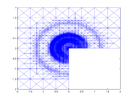
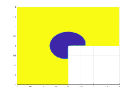
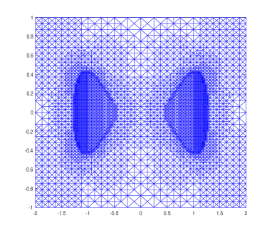
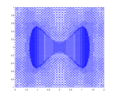
Pointwise A Posteriori Error Analysis of a Discontinuous Galerkin Method for the Elliptic Obstacle Problem

Blanca Ayuso de Dios Dipartimento di Matematica e Applicazioni, Università di Milano Bicocca, Via Cozzi 55, 20125 Milano, Italy, & Istituto di Matematica Applicata e Tecnologie Informatiche Enrico Magenes del C.N.R., via Ferrata, 27100, Pavia, Italy blanca.ayuso@unimib.it Thirupathi Gudi Department of Mathematics, Indian Institute of Science, Bangalore - 560012 gudi@math.iisc.ernet.in  and  Kamana Porwal Department of Mathematics, Indian Institute of Technology Delhi - 110016 kamana@maths.iitd.ac.in
Abstract.

We present a posteriori error analysis in the supremum norm for the symmetric interior penalty discontinuous Galerkin method for the elliptic obstacle problem. We construct discrete barrier functions based on appropriate corrections of the conforming part of the solution that is obtained via a constrained averaging operator. The corrector function accounts properly for the non-conformity of the approximation and it is estimated by direct use of the Green’s function of the unconstrained elliptic problem. The use of the continuous maximum principle guarantees the validity of the analysis without mesh restrictions but shape regularity. The proposed residual type estimators are shown to be reliable and efficient. Numerical results in two dimensions are included to verify the theory and validate the performance of the error estimator.

Key words and phrases:
finite element, discontinuous Galerkin, a posteriori error estimate, obstacle problem, variational inequalities, Lagrange multiplier, pointwise
1991 Mathematics Subject Classification:
65N30, 65N15
The third author’s work is supported in part by The SERB-MATRICS grant and in part by IITD SEED grant

1. Introduction

Several problems in a variety of fields of science (Physics, Biology, Industry, Finance, Geometry to mention a few) are often described by partial differential equations (PDEs) that exhibit a-priori unknown interfaces or boundaries. They are typically called free boundary problems and constitute an important line of research for the mathematical and the numerical analysis communities.
Among these problems, the most classical one is the elliptic obstacle problem that arises in diverse applications in elasticity, fluid dynamics and operations research, to name a few[14, 33, 25]. It is also a prototype of the elliptic variational inequalities of the first kind. It’s variational formulation reads: find u𝒦𝑢𝒦u\in\mathcal{K} such that

(1.1) Ωu(uv)dx(f,uv)v𝒦,formulae-sequencesubscriptΩ𝑢𝑢𝑣𝑑𝑥𝑓𝑢𝑣for-all𝑣𝒦\int_{\Omega}\nabla u\cdot\nabla(u-v)\,dx\leq(f,u-v)\quad\forall v\in\mathcal{K},

where Ωd,d=2,3formulae-sequenceΩsuperscript𝑑𝑑23\Omega\subset\mathbb{R}^{d},~{}d=2,3 is a bounded, polygonal (d=2𝑑2d=2) or polyhedral (d=3𝑑3d=3) domain with boundary ΩΩ\partial\Omega, fL(Ω)𝑓superscript𝐿Ωf\in L^{\infty}(\Omega) denotes the force and (,)(\cdot,\cdot) refers to the L2(Ω)superscript𝐿2ΩL^{2}(\Omega) inner-product. For any 1r1𝑟1\leq r\leq\infty and DΩ𝐷ΩD\subset\Omega, we denote the Lr(D)superscript𝐿𝑟𝐷L^{r}(D) norm by Lr(D)\|\cdot\|_{L^{r}(D)}. The set Dosuperscript𝐷𝑜D^{o} denotes the interior of D for any set DΩ𝐷ΩD\subset\Omega. We further use standard notations of Sobolev spaces [1, Chapter 3]. The associated norm on Sobolev space Wm,r(Ω)superscript𝑊𝑚𝑟ΩW^{m,r}(\Omega) is denoted by Wm,r\|\cdot\|_{W^{m,r}} and semi-norm by ||Wm,r|\cdot|_{W^{m,r}}. The Sobolev space Wm,r(Ω)superscript𝑊𝑚𝑟ΩW^{m,r}(\Omega) with m=0𝑚0m=0 will denote the standard Lr(Ω)superscript𝐿𝑟ΩL^{r}(\Omega) space. The set of admissible displacements 𝒦𝒦\mathcal{K} is a non-empty, closed and convex set defined by

(1.2) 𝒦:={vV:vχa.e. inΩ},assign𝒦conditional-set𝑣𝑉𝑣𝜒a.e. inΩ\mathcal{K}:=\{v\in V:v\geq\chi\;\;\text{a.e. in}\;\;\Omega\},

with V:=H01(Ω)assign𝑉subscriptsuperscript𝐻10ΩV:=H^{1}_{0}(\Omega) and χH1(Ω)C0,α(Ω¯),0<α1formulae-sequence𝜒superscript𝐻1Ωsuperscript𝐶0𝛼¯Ω0𝛼1\chi\in H^{1}(\Omega)\cap C^{0,\alpha}(\overline{\Omega}),\quad 0<\alpha\leq 1 denoting the obstacle which satisfies the compatibility condition χ0𝜒0\chi\leq 0 on ΩΩ\partial\Omega. In (1.1), the solution u𝑢u could be regarded as the equilibrium position of an elastic membrane subject to the load f𝑓f whose boundary is held fixed (uH01(Ω)𝑢subscriptsuperscript𝐻10Ωu\in H^{1}_{0}(\Omega)) and which is constrained to lie above the given obstacle χ𝜒\chi. Such constraint results in non-linearity inherent to the underlying PDE, the Poisson equation here. The classical theory of Stampacchia [25, Chapter 1, page 4], [33, Chapter 2, page 40] guarantees the existence and uniqueness of the solution. As for the regularity of the solution, it is shown in [21, 11], that under our assumptions on the domain and the data, fL(Ω)𝑓superscript𝐿Ωf\in L^{\infty}(\Omega) and χH1(Ω)C0,α(Ω¯),0<α1formulae-sequence𝜒superscript𝐻1Ωsuperscript𝐶0𝛼¯Ω0𝛼1\chi\in H^{1}(\Omega)\cap C^{0,\alpha}(\overline{\Omega}),~{}~{}0<\alpha\leq 1, the solution to the variational inequality (1.1) is also Hölder continuous i.e. we have uH01(Ω)C0,β(Ω¯)𝑢superscriptsubscript𝐻01Ωsuperscript𝐶0𝛽¯Ωu\in H_{0}^{1}(\Omega)\cap C^{0,\beta}(\overline{\Omega}) for 0<βα0𝛽𝛼0<\beta\leq\alpha.

The contact (or coincidence) and non-contact sets of the exact solution u𝑢u are defined as

(1.3) \displaystyle\mathbb{C} :={xΩ:u(x)=χ(x)}o,assignabsentsuperscriptconditional-set𝑥Ω𝑢𝑥𝜒𝑥𝑜\displaystyle:=\left\{x\in\Omega:u(x)=\chi(x)\right\}^{o},
\displaystyle\mathbb{N} :={xΩ:u(x)>χ(x)}.assignabsentconditional-set𝑥Ω𝑢𝑥𝜒𝑥\displaystyle:=\left\{x\in\Omega:u(x)>\chi(x)\right\}.

The free boundary here is the interior boundary of the coincidence set \mathbb{C}. The Hölder continuity of u𝑢u guarantees that both \mathbb{C} and the free boundary are closed sets.

From Riesz representation theorem, associated to the solution u𝑢u we introduce the linear functional σ(u)H1(Ω)𝜎𝑢superscript𝐻1Ω\sigma(u)\in H^{-1}(\Omega) by

(1.4) σ(u),v=(f,v)a(u,v),vH01(Ω),formulae-sequence𝜎𝑢𝑣𝑓𝑣𝑎𝑢𝑣for-all𝑣subscriptsuperscript𝐻10Ω\displaystyle\langle\sigma(u),v\rangle=(f,v)-a(u,v),\quad\forall v\in H^{1}_{0}(\Omega),

where ,\langle\cdot,\cdot\rangle refers to the duality pairing of H1(Ω)superscript𝐻1ΩH^{-1}(\Omega) and H01(Ω)subscriptsuperscript𝐻10ΩH^{1}_{0}(\Omega). From (1.4) and (1.1), it follows that

(1.5) σ(u),vu0,v𝒦.formulae-sequence𝜎𝑢𝑣𝑢0for-all𝑣𝒦\langle\sigma(u),v-u\rangle\leq 0,\quad\forall v\in\mathcal{K}.

In particular111 Choosing 0ϕH01(Ω)0italic-ϕsuperscriptsubscript𝐻01Ω0\leq\phi\in H_{0}^{1}(\Omega) and setting v=u+ϕ𝑣𝑢italic-ϕv=u+\phi in (1.5), we get σ(u)0𝜎𝑢0\sigma(u)\leq 0. Further, if u>χ𝑢𝜒u>\chi on some open set DΩ𝐷ΩD\subset\Omega then σ(u)=0𝜎𝑢0\sigma(u)=0 on D𝐷D (see [33, Chapter 2, page 44]) , σ(u)=0𝜎𝑢0\sigma(u)=0 on the non-contact set \mathbb{N} and the support of σ(u)𝜎𝑢\sigma(u) is contained in the contact set \mathbb{C}. In fact, [33, Chapter II, Section 6] the Riesz representation theorem states that there is a finite non-negative radon measure dσ𝑑𝜎-d\sigma supported on \mathbb{C} satisfying:

σ(u),v=Ωv𝑑σ=(f,v)a(u,v)vC0(Ω¯),formulae-sequence𝜎𝑢𝑣subscriptΩ𝑣differential-d𝜎𝑓𝑣𝑎𝑢𝑣for-all𝑣subscript𝐶0¯Ω\langle\sigma(u),v\rangle=\int_{\Omega}vd\sigma=(f,v)-a(u,v)\qquad\forall\,v\in C_{0}(\bar{\Omega}),

where C0(Ω¯)subscript𝐶0¯ΩC_{0}(\bar{\Omega}) denotes the space of continuous functions on Ω¯¯Ω\bar{\Omega} with compact support. Often, σ(u)𝜎𝑢\sigma(u) is also referred as the continuous Lagrange multiplier. We wish to stress that the solution operator of (1.1) is not only non-linear and non-differentiable, but also strikingly not one-to-one in the sense that any variation in f𝑓f within the contact set might or might not result in a variation in the solution u𝑢u.

A-priori error analysis in the energy norm for (1.1) are discussed in [19, 9, 10, 44, 22] for conforming methods and in [43] for DG methods. In energy norm, several a-posteriori error estimators are studied in  [5, 13, 6, 42, 35, 29, 23] for conforming approximation of variational inequalities while residual type a posteriori error estimators have been derived in [27, 28] for DG approximation. In this article, we study a-posteriori error analysis in the supremum norm, for the symmetric interior penalty discontinuous Galerkin (SIPG) approximation of the elliptic obstacle problem (1.1). The rationality of our choice of norm comes from the fact that estimates in the maximum norm are relevant for variational inequalities since they provide further localized information on the approximation. Moreover, they also constitute a cornerstone for a future subsequent convergence analysis of the free boundary [8, 36].

A-priori error analysis in Lsuperscript𝐿L^{\infty} norm goes back to the seminal works by Baiocchi and Nitsche [4, 34], for conforming finite linear finite elements. As the proof uses a discrete maximum principle, the analysis requires the classical assumption on acute angles for the mesh partitions [14]. Unlike for a-priori analysis, in [39, 40] the authors accomplish the Lsuperscript𝐿L^{\infty} norm a-posteriori analysis of the obstacle problem, by using a dual approach to Baiocchi [4] and making use of the continuous maximum principle, hence avoiding any mesh restriction except the standard shape regularity. In [39], a positivity preserving interpolation operator is used and in [40] the estimators and the analysis is refined to ensure further localization of the estimators. The ideas in [39, 40] have been extended in [38] to the conforming approximation of monotone semi-linear equations and in [20], for the conforming approximation of a double obstacle problem arising from regularized minimization of a related functional, providing a uniform error estimator with respect to the regularization parameter that can be further used in the minimization of the discrete functional. We also refer to the nice survey [37] for the approximation of classical and fractional obstacle problems.

In this work, we follow the path laid down in [39, 40], extending it and adapting it for the SIPG method. We stress that the nonconformity of the approximation and the nonlinearity of the problem, preclude the extension from being trivial. Also, the discontinuous nature of the finite element space allow for a slightly better localization of the error estimators. To be able to use the continuous maximum principle, which permits to avoid mesh restrictions, we construct discrete barrier functions for the solution u𝑢u that belong to H1superscript𝐻1H^{1}. This in turn, forces us to construct the discrete sub and super-solutions starting from the conforming part of the DG approximation and amend it with some corrector function that account for the nonconformity of our approximation. The conforming part of the DG approximation is obtained by using an averaging operator introduced in [27] that ensures the obstacle constraint are preserved. The proof of the reliability of the estimator relies then on providing a pointwise estimate on the corrector function. Here, our approach varies from [39, 40] where a regularized Greens’ function (for the unconstrained elliptic problem) is employed. Instead, we consider the direct use of Greens’ functions catering for the sharpened estimates (on the Greens’ function) proved in [16, 17]. As a result, the final estimators are improved in the exponent of the logarithmic factor with respect to [39], but more significantly, this approach allows for accounting appropriately the non-conformity in the approximation and evidences that the analysis performed for SIPG method, cannot be extended to any of the non-symmetric methods of the interior penalty family. The local efficiency estimates of the error estimator are obtained using the bubble functions techniques [3]. To prove the efficiency of the estimator term that measures the error in approximation of the obstacle in the discrete contact set and discrete free boundary set, unlike in [39, 40] we need to assume χ<0𝜒0\chi<0 on the part of ΩΩ\partial\Omega that intersects the free boundary. This assumption is not very restrictive and is done in many research works. We accept this technical restriction in order to keep the locality of the definition of the discrete Lagrange multiplier granted by the DG construction, which is computationally simpler than the ones introduced in [39, 40]. Numerical experiments in two dimensions confirming the applicability of a posteriori estimates within adaptive schemes are presented.

We expect that the analysis presented could be helpful in understanding the convergence of the DG approximation to the free boundary, taking into account the seminal works [8, 36]. This would allow to assess if the often acclaimed flexibility of DG methods could bring any real benefit with respect to the conforming approximation in this context. This will be the subject of future research. The ideas developed here might be used in the analysis of DG approximation of control problems as well as the a-posteriori error analysis of DG methods for other variational inequalities e.g. Signorini problem [25]. The error estimator obtained in this article improves the error estimator obtained in [39] by a logarithm factor when applied to the conforming finite element methods. Except for this logarithm term, our error estimator is comparable to that of [39].

The article is organized as follows. In the next section we introduce basic notations and some auxiliary results that will be used in further analysis. DG method for approximating the elliptic obstacle problem (1.1) and its main properties are discussed in Section 3. In Section 4, we introduce the error estimators which are the main tools for the analysis and prove the major result of the paper, namely the reliability of the estimator. The efficiency of a posteriori error estimator is discussed in Section 5. Numerical experiments are presented illustrating the theoretical findings and validating the performance of the estimator in Section 6.

2. Notation and Preliminary Results

In this section, we introduce useful notations and some auxiliary results which will be used throughout this work.

𝒯hsubscript𝒯\displaystyle\mathcal{T}_{h} =a simplicial triangulations of Ω,that are assumed to be shape regularabsenta simplicial triangulations of Ωthat are assumed to be shape regular\displaystyle=\text{a simplicial triangulations of }\Omega,\text{that are assumed to be shape regular}
T𝑇\displaystyle T =an element of 𝒯h,|T|=volume of the simplexTformulae-sequenceabsentan element of subscript𝒯𝑇volume of the simplex𝑇\displaystyle=\text{an element of }\mathcal{T}_{h},\qquad|T|=\text{volume of the simplex}~{}T
hTsubscript𝑇\displaystyle h_{T} =diameter of T,h=max{hT:T𝒯h},hmin=min{hT:T𝒯h}formulae-sequenceabsentdiameter of 𝑇formulae-sequence:subscript𝑇𝑇subscript𝒯subscript𝑚𝑖𝑛:subscript𝑇𝑇subscript𝒯\displaystyle=\text{diameter of }T,\qquad h=\max\{h_{T}:T\in\mathcal{T}_{h}\},\qquad h_{min}=\min\{h_{T}:T\in\mathcal{T}_{h}\}
𝒱hisuperscriptsubscript𝒱𝑖\displaystyle\mathcal{V}_{h}^{i} =set of all vertices in 𝒯h that are in Ωabsentset of all vertices in subscript𝒯 that are in Ω\displaystyle=\text{set of all vertices in }\mathcal{T}_{h}\text{ that are in }\Omega
𝒱hbsuperscriptsubscript𝒱𝑏\displaystyle\mathcal{V}_{h}^{b} =set of all vertices in 𝒯h that are on Ωabsentset of all vertices in subscript𝒯 that are on Ω\displaystyle=\text{set of all vertices in }\mathcal{T}_{h}\text{ that are on }\partial\Omega
𝒱hsubscript𝒱\displaystyle\mathcal{V}_{h} =𝒱hi𝒱hbabsentsuperscriptsubscript𝒱𝑖superscriptsubscript𝒱𝑏\displaystyle=\mathcal{V}_{h}^{i}\cup\mathcal{V}_{h}^{b}
𝒱Tsubscript𝒱𝑇\displaystyle\mathcal{V}_{T} =set of three vertices of simplexTabsentset of three vertices of simplex𝑇\displaystyle=\text{set of three vertices of simplex}~{}T
hosubscriptsuperscript𝑜\displaystyle{{\mathcal{E}}^{o}_{h}} =set of all interior edges/faces of 𝒯habsentset of all interior edges/faces of subscript𝒯\displaystyle=\text{set of all interior edges/faces of }\mathcal{T}_{h}
hsubscriptsuperscript\displaystyle{{\mathcal{E}}^{\partial}_{h}} =set of all boundary edges/faces of 𝒯habsentset of all boundary edges/faces of subscript𝒯\displaystyle=\text{set of all boundary edges/faces of }\mathcal{T}_{h}
hsubscript\displaystyle\mathcal{E}_{h} =hohabsentsubscriptsuperscript𝑜subscriptsuperscript\displaystyle={{\mathcal{E}}^{o}_{h}}\cup{{\mathcal{E}}^{\partial}_{h}}
hesubscript𝑒\displaystyle h_{e} =diameter of any edge/face ehabsentdiameter of any edge/face 𝑒subscript\displaystyle=\text{diameter of any edge/face }e\in\mathcal{E}_{h}
𝒯psubscript𝒯𝑝\displaystyle\mathcal{T}_{p} =set of all elements sharing the vertex pabsentset of all elements sharing the vertex 𝑝\displaystyle=\text{set of all elements sharing the vertex }p
𝒯esubscript𝒯𝑒\displaystyle\mathcal{T}_{e} =patch of two elements sharing the face ehoi.e.𝒯e={T+,T},whereT+andTare twoformulae-sequenceabsentpatch of two elements sharing the face 𝑒subscriptsuperscript𝑜i.e.subscript𝒯𝑒subscript𝑇subscript𝑇wheresubscript𝑇andsubscript𝑇are two\displaystyle=\text{patch of two elements sharing the face }e\in{{\mathcal{E}}^{o}_{h}}~{}\text{i.e.}~{}\mathcal{T}_{e}=\{T_{+},T_{-}\},\text{where}~{}T_{+}~{}\text{and}~{}T_{-}~{}\text{are two}
elements sharing the faceeelements sharing the face𝑒\displaystyle\quad\text{elements sharing the face}~{}e
psubscript𝑝\displaystyle\mathcal{E}_{p} =set of all edges/faces connected to the vertex pabsentset of all edges/faces connected to the vertex 𝑝\displaystyle=\text{set of all edges/faces connected to the vertex }p
hsubscript\displaystyle\nabla_{h} =piecewise (element-wise) gradient.absentpiecewise (element-wise) gradient\displaystyle=\text{piecewise (element-wise) gradient}.

For any T𝒯h,p𝒱hformulae-sequence𝑇subscript𝒯𝑝subscript𝒱T\in\mathcal{T}_{h},~{}p\in\mathcal{V}_{h} and eho𝑒subscriptsuperscript𝑜e\in{{\mathcal{E}}^{o}_{h}}, we define,

(2.1) ωTsubscript𝜔𝑇\displaystyle\omega_{T} :={T𝒯h:TT}assignabsentconditional-setsuperscript𝑇subscript𝒯superscript𝑇𝑇\displaystyle:=\cup\left\{T^{\prime}\in\mathcal{T}_{h}\,\,:\,\,T^{\prime}\cap T\neq\emptyset\right\}
(2.2) ωpsubscript𝜔𝑝\displaystyle\omega_{p} :={T𝒯h:T𝒯p}assignabsentconditional-setsuperscript𝑇subscript𝒯superscript𝑇subscript𝒯𝑝\displaystyle:=\cup\{T^{\prime}\in\mathcal{T}_{h}\,\,:T^{\prime}\in\mathcal{T}_{p}\}
(2.3) ωesubscript𝜔𝑒\displaystyle\omega_{e} :=T+T.assignabsentsubscript𝑇subscript𝑇\displaystyle:=T_{+}\cup T_{-}\qquad.

Further,

  • For any function v𝑣v, v+superscript𝑣v^{+} denotes it’s positive part i.e. v+(x)=max{v(x),0}superscript𝑣𝑥𝑣𝑥0v^{+}(x)=\max\{v(x),0\}

  • For any function v𝑣v, supp(v)𝑠𝑢𝑝𝑝𝑣supp(v) denotes support of the function v𝑣v

  • L(h):=maxehL(e)\|\cdot\|_{L^{\infty}(\mathcal{E}_{h})}:=\displaystyle\max_{e\in\mathcal{E}_{h}}\|\cdot\|_{L^{\infty}(e)}

  • L(𝒯h):=maxT𝒯hL(T)\|\cdot\|_{L^{\infty}(\mathcal{T}_{h})}:=\displaystyle\max_{T\in\mathcal{T}_{h}}\|\cdot\|_{L^{\infty}(T)}

  • XYless-than-or-similar-to𝑋𝑌X\lesssim Y: there exist a positive constant C𝐶C, independent of mesh parameter and the solution such that XCY𝑋𝐶𝑌X\leq CY.

The shape regularity assumption on 𝒯hsubscript𝒯\mathcal{T}_{h} [14, Chapter 3, page 124] implies that

|p|1p𝒱h,formulae-sequenceless-than-or-similar-tosubscript𝑝1for-all𝑝subscript𝒱|\mathcal{E}_{p}|\lesssim 1\quad\forall p\in\mathcal{V}_{h},

where |p|subscript𝑝|\mathcal{E}_{p}| denotes the cardinality of psubscript𝑝{\mathcal{E}_{p}}.

In order to define the jump and mean of discontinuous functions appropriately, we introduce the broken Sobolev space

H1(Ω,𝒯h)={vL2(Ω):vT=v|TH1(T)T𝒯h}.superscript𝐻1Ωsubscript𝒯conditional-set𝑣superscript𝐿2Ωformulae-sequencesubscript𝑣𝑇evaluated-at𝑣𝑇superscript𝐻1𝑇for-all𝑇subscript𝒯\displaystyle H^{1}(\Omega,\mathcal{T}_{h})=\{v\in L^{2}(\Omega):\,v_{{\scriptscriptstyle T}}=v|_{T}\in H^{1}(T)\quad\forall\,~{}T\in{\mathcal{T}}_{h}\}.

Trace Operators: Let eho𝑒subscriptsuperscript𝑜e\in{{\mathcal{E}}^{o}_{h}} be shared by two elements T+subscript𝑇T_{+} and Tsubscript𝑇T_{-} such that e=T+T𝑒subscript𝑇subscript𝑇e=\partial T_{+}\cap\partial T_{-}. If n+subscript𝑛n_{+} is the unit normal of e𝑒e pointing from T+subscript𝑇T_{+} to Tsubscript𝑇T_{-} then n=n+subscript𝑛subscript𝑛n_{-}=-n_{+}. We set v±=v|T±subscript𝑣plus-or-minusevaluated-at𝑣subscript𝑇plus-or-minusv_{\pm}=v\big{|}_{T_{\pm}} and define the jump and the mean of vH1(Ω,𝒯h)𝑣superscript𝐻1Ωsubscript𝒯v\in H^{1}(\Omega,{\mathcal{T}}_{h}) on e𝑒e by

[[v]]=v+n++vnand{{v}}=12(v++v),respectively.formulae-sequencedelimited-[]delimited-[]𝑣subscript𝑣subscript𝑛subscript𝑣subscript𝑛and𝑣12subscript𝑣subscript𝑣respectively.\displaystyle[\hskip-1.5pt[v]\hskip-1.5pt]=v_{+}n_{+}+v_{-}n_{-}\,\quad\mbox{and}\,\quad\{\hskip-3.0pt\{v\}\hskip-3.0pt\}=\frac{1}{2}(v_{+}+v_{-}),\quad\mbox{respectively.}

Similarly for a vector valued function qH1(Ω,𝒯h)d𝑞superscript𝐻1superscriptΩsubscript𝒯𝑑q\in H^{1}(\Omega,{\mathcal{T}}_{h})^{d}, the jump and mean on eho𝑒subscriptsuperscript𝑜e\in{{\mathcal{E}}^{o}_{h}} are defined by

[[q]]=q+n++qnand{{q}}=12(q++q).formulae-sequencedelimited-[]delimited-[]𝑞subscript𝑞subscript𝑛subscript𝑞subscript𝑛and𝑞12subscript𝑞subscript𝑞\displaystyle[\hskip-1.5pt[q]\hskip-1.5pt]=q_{+}\cdot n_{+}+q_{-}\cdot n_{-}\quad\,\mbox{and}\quad\,\{\hskip-3.0pt\{q\}\hskip-3.0pt\}=\frac{1}{2}(q_{+}+q_{-}).

For a boundary face eh𝑒subscriptsuperscripte\in{{\mathcal{E}}^{\partial}_{h}}, with nesubscript𝑛𝑒n_{e} denoting the unit normal of e𝑒e that points outward to T𝑇T for TΩ=e𝑇Ω𝑒\partial T\cap\partial\Omega=e, we set:

[[v]]=vneand{{v}}=v,vH1(T),formulae-sequencedelimited-[]delimited-[]𝑣𝑣subscript𝑛𝑒andformulae-sequence𝑣𝑣for-all𝑣superscript𝐻1𝑇\displaystyle[\hskip-1.5pt[v]\hskip-1.5pt]=vn_{e}\,\quad\mbox{and}\,\quad\{\hskip-3.0pt\{v\}\hskip-3.0pt\}=v,\quad\forall\,v\in H^{1}(T),
[[q]]=wne,and{{q}}=q,qH1(T)d.formulae-sequencedelimited-[]delimited-[]𝑞𝑤subscript𝑛𝑒formulae-sequenceand𝑞𝑞for-all𝑞superscript𝐻1superscript𝑇𝑑\displaystyle[\hskip-1.5pt[q]\hskip-1.5pt]=w\cdot n_{e},\,\,\mbox{and}\,\,\{\hskip-3.0pt\{q\}\hskip-3.0pt\}=q,\quad\forall\,q\in H^{1}(T)^{d}.

Throughout the article, C𝐶C denotes a generic positive constant which is independent of the mesh size hh.
Discrete Spaces: Let k(T)superscript𝑘𝑇\mathbb{P}^{k}(T), k0𝑘0k\geq 0 integer, is the space of polynomials defined on T𝑇T of degree less than or equal to k𝑘k. We define the first order discontinuous finite element space as

Vh={vL2(Ω):v|T1(T),T𝒯h}.subscript𝑉conditional-set𝑣superscript𝐿2Ωformulae-sequenceevaluated-at𝑣𝑇superscript1𝑇𝑇subscript𝒯\displaystyle V_{h}=\{v\in L^{2}(\Omega):v|_{T}\in\mathbb{P}^{1}(T),\,T\in\mathcal{T}_{h}\}.

The conforming finite element space, denoted here by Vhconfsuperscriptsubscript𝑉𝑐𝑜𝑛𝑓V_{h}^{conf} is then defined as

Vhconf=VhH01(Ω).superscriptsubscript𝑉𝑐𝑜𝑛𝑓subscript𝑉superscriptsubscript𝐻01ΩV_{h}^{conf}=V_{h}\cap H_{0}^{1}(\Omega).

Let χhVhconfsubscript𝜒superscriptsubscript𝑉𝑐𝑜𝑛𝑓\chi_{h}\in V_{h}^{conf} be the nodal interpolation of χ𝜒\chi. We define the discrete analogue of 𝒦𝒦\mathcal{K} by

(2.4) 𝒦h:={vhVh:vh|T(p)χh(p),p𝒱T,T𝒯h},assignsubscript𝒦conditional-setsubscript𝑣subscript𝑉formulae-sequenceevaluated-atsubscript𝑣𝑇𝑝subscript𝜒𝑝formulae-sequencefor-all𝑝subscript𝒱𝑇for-all𝑇subscript𝒯\mathcal{K}_{h}:=\{v_{h}\in V_{h}:v_{h}|_{T}(p)\geq\chi_{h}(p),\;\;\forall p\in\mathcal{V}_{T},\;\;\forall T\in\mathcal{T}_{h}\},

which is a nonempty, closed and convex subset of Vhsubscript𝑉V_{h}. Note however that, since χ𝜒\chi is a general function, we have 𝒦h𝒦not-subset-of-nor-equalssubscript𝒦𝒦\mathcal{K}_{h}\nsubseteq\mathcal{K}. In case of χ𝜒\chi being an affine function, we have 𝒦hH01(Ω)𝒦subscript𝒦superscriptsubscript𝐻01Ω𝒦\mathcal{K}_{h}\cap H_{0}^{1}(\Omega)\subseteq\mathcal{K}.

2.1. Some Discrete Operators

We now introduce some discrete operators that will be used in further analysis.
Following [16], we define a local projection operator Πh:L1(Ω)Vh:subscriptΠsuperscript𝐿1Ωsubscript𝑉\Pi_{h}:L^{1}(\Omega)\longrightarrow V_{h}. For any T𝒯h𝑇subscript𝒯T\in\mathcal{T}_{h}, let (ϕpT)p𝒱Tsubscriptsuperscriptsubscriptitalic-ϕ𝑝𝑇𝑝subscript𝒱𝑇(\phi_{p}^{T})_{p\in\mathcal{V}_{T}} be associated Lagrange basis functions. Then, for any vL1(T)𝑣superscript𝐿1𝑇v\in L^{1}(T), we define ΠhT:L1(T)Vh:superscriptsubscriptΠ𝑇superscript𝐿1𝑇subscript𝑉\Pi_{h}^{T}:L^{1}(T)\longrightarrow V_{h} by

(2.5) ΠhTv(x):=p𝒱TϕpT(x)TψpT(s)v(s)𝑑s,assignsuperscriptsubscriptΠ𝑇𝑣𝑥subscript𝑝subscript𝒱𝑇superscriptsubscriptitalic-ϕ𝑝𝑇𝑥subscript𝑇superscriptsubscript𝜓𝑝𝑇𝑠𝑣𝑠differential-d𝑠\Pi_{h}^{T}v(x):=\sum_{p\in\mathcal{V}_{T}}\phi_{p}^{T}(x)\int_{T}\psi_{p}^{T}(s)v(s)~{}ds,

where (ψpT)p𝒱Tsubscriptsuperscriptsubscript𝜓𝑝𝑇𝑝subscript𝒱𝑇(\psi_{p}^{T})_{p\in\mathcal{V}_{T}} is the L2(T)superscript𝐿2𝑇L^{2}(T) dual basis of (ϕpT)p𝒱Tsubscriptsuperscriptsubscriptitalic-ϕ𝑝𝑇𝑝subscript𝒱𝑇(\phi_{p}^{T})_{p\in\mathcal{V}_{T}} i.e.

TϕpT(x)ψqT(x)𝑑x=δpq,p,q𝒱T.formulae-sequencesubscript𝑇superscriptsubscriptitalic-ϕ𝑝𝑇𝑥superscriptsubscript𝜓𝑞𝑇𝑥differential-d𝑥subscript𝛿𝑝𝑞𝑝𝑞subscript𝒱𝑇\displaystyle\int_{T}\phi_{p}^{T}(x)\psi_{q}^{T}(x)~{}dx=\delta_{pq},\quad p,q\in\mathcal{V}_{T}.

Then, ΠhsubscriptΠ\Pi_{h} is defined by setting Πhv|T=ΠhTvevaluated-atsubscriptΠ𝑣𝑇superscriptsubscriptΠ𝑇𝑣\Pi_{h}v|_{T}=\Pi_{h}^{T}v for each T𝒯h𝑇subscript𝒯T\in\mathcal{T}_{h}. Observe that from (2.5) we do have ΠhTϕpT=ϕpTsuperscriptsubscriptΠ𝑇superscriptsubscriptitalic-ϕ𝑝𝑇superscriptsubscriptitalic-ϕ𝑝𝑇\Pi_{h}^{T}\phi_{p}^{T}=\phi_{p}^{T} which implies ΠhTsuperscriptsubscriptΠ𝑇\Pi_{h}^{T} is indeed a projection, and so is ΠhsubscriptΠ\Pi_{h}. Hence we have Πhvh=vhsubscriptΠsubscript𝑣subscript𝑣\Pi_{h}v_{h}=v_{h} for all vhVhsubscript𝑣subscript𝑉v_{h}\in V_{h}.

The following Lemma from [16] provides stability and approximation properties of ΠhTsubscriptsuperscriptΠ𝑇\Pi^{T}_{h}. It’s proof follows by using Bramble Hilbert lemma and standard scaling arguments; see [16] for details.

Lemma 2.1.

Let T𝒯h𝑇subscript𝒯T\in\mathcal{T}_{h} and let ΠhT:L1(T)Vh:superscriptsubscriptΠ𝑇superscript𝐿1𝑇subscript𝑉\Pi_{h}^{T}:L^{1}(T)\longrightarrow V_{h} be the local projection defined in (2.5). Let s𝑠s be an integer such that 0s20𝑠20\leq s\leq 2 and ψWs,1(T)𝜓superscript𝑊𝑠1𝑇\psi\in W^{s,1}(T). Then,

(2.6) |ΠTψ|Ws,1(T)subscriptsuperscriptΠ𝑇𝜓superscript𝑊𝑠1𝑇\displaystyle|\Pi^{T}\psi|_{W^{s,1}(T)} |ψ|Ws,1(T),0s2formulae-sequenceless-than-or-similar-toabsentsubscript𝜓superscript𝑊𝑠1𝑇0𝑠2\displaystyle\lesssim|\psi|_{W^{s,1}(T)},\qquad 0\leq s\leq 2
(2.7) k=0shTks|ψΠhTψ|Wk,1(T)superscriptsubscript𝑘0𝑠superscriptsubscript𝑇𝑘𝑠subscript𝜓subscriptsuperscriptΠ𝑇𝜓superscript𝑊𝑘1𝑇\displaystyle\sum_{k=0}^{s}h_{T}^{k-s}|\psi-\Pi^{T}_{h}\psi|_{W^{k,1}(T)} |ψ|Ws,1(T),0s2.formulae-sequenceless-than-or-similar-toabsentsubscript𝜓superscript𝑊𝑠1𝑇0𝑠2\displaystyle\lesssim|\psi|_{W^{s,1}(T)},\qquad 0\leq s\leq 2.

We now revise the following inverse and trace inequalities which will be frequently used in our later analysis.
Inverse Inequalities [14, Chapter 3, page 140]: For any vhVhsubscript𝑣subscript𝑉v_{h}\in V_{h} and 1p,qformulae-sequence1𝑝𝑞1\leq p\,,q\leq\infty,

(2.8) vhWm,p(T)subscriptnormsubscript𝑣superscript𝑊𝑚𝑝𝑇\displaystyle\|v_{h}\|_{W^{m,p}(T)} hTmhTd(1p1q)vhW,q(T)less-than-or-similar-toabsentsuperscriptsubscript𝑇𝑚superscriptsubscript𝑇𝑑1𝑝1𝑞subscriptnormsubscript𝑣superscript𝑊𝑞𝑇\displaystyle\lesssim h_{T}^{\ell-m}h_{T}^{d\left(\frac{1}{p}-\frac{1}{q}\right)}\|v_{h}\|_{W^{\ell,q}(T)}\quad T𝒯h,for-all𝑇subscript𝒯\displaystyle\forall\,T\in\mathcal{T}_{h},
(2.9) vhLp(T)subscriptnormsubscript𝑣superscript𝐿𝑝𝑇\displaystyle\|\nabla v_{h}\|_{L^{p}(T)} hT1vhLp(T)less-than-or-similar-toabsentsuperscriptsubscript𝑇1subscriptnormsubscript𝑣superscript𝐿𝑝𝑇\displaystyle\lesssim h_{T}^{-1}\|v_{h}\|_{L^{p}(T)}\quad T𝒯h,for-all𝑇subscript𝒯\displaystyle\forall\,T\in\mathcal{T}_{h},
(2.10) vhL(T)subscriptnormsubscript𝑣superscript𝐿𝑇\displaystyle\|v_{h}\|_{L^{\infty}(T)} hTd2vhL2(T)less-than-or-similar-toabsentsuperscriptsubscript𝑇𝑑2subscriptnormsubscript𝑣superscript𝐿2𝑇\displaystyle\lesssim h_{T}^{-\frac{d}{2}}\|v_{h}\|_{L^{2}(T)}\quad T𝒯h,for-all𝑇subscript𝒯\displaystyle\forall\,T\in\mathcal{T}_{h},
(2.11) vhL(e)subscriptnormsubscript𝑣superscript𝐿𝑒\displaystyle\|v_{h}\|_{L^{\infty}(e)} he1d2vhL2(e)less-than-or-similar-toabsentsuperscriptsubscript𝑒1𝑑2subscriptnormsubscript𝑣superscript𝐿2𝑒\displaystyle\lesssim h_{e}^{\frac{1-d}{2}}\|v_{h}\|_{L^{2}(e)}\quad eh,for-all𝑒subscript\displaystyle\forall\,e\in{{\mathcal{E}}_{h}},

where hesubscript𝑒h_{e} and hTsubscript𝑇h_{T} denote, respectively, the diameters of the face e𝑒e and the element T𝑇T.

Trace inequality [2]: Let ψW1,p(T),T𝒯hformulae-sequence𝜓superscript𝑊1𝑝𝑇𝑇subscript𝒯\psi\in W^{1,p}(T),~{}~{}~{}T\in\mathcal{T}_{h} and let eh𝑒subscripte\in\mathcal{E}_{h} be an edge/face of T𝑇T. Then for any 1p<1𝑝1\leq p<\infty, it holds that

(2.12) ψLp(e)phe1(ψLp(T)p+hepψLp(T)p),less-than-or-similar-tosuperscriptsubscriptnorm𝜓superscript𝐿𝑝𝑒𝑝superscriptsubscript𝑒1superscriptsubscriptnorm𝜓superscript𝐿𝑝𝑇𝑝superscriptsubscript𝑒𝑝superscriptsubscriptnorm𝜓superscript𝐿𝑝𝑇𝑝\|\psi\|_{L^{p}(e)}^{p}\lesssim h_{e}^{-1}\big{(}\|\psi\|_{L^{p}(T)}^{p}+h_{e}^{p}\|\nabla\psi\|_{L^{p}(T)}^{p}\big{)},

where hesubscript𝑒h_{e} denotes the diameter of the face e𝑒e.

Averaging or Enriching Operator: We close the section by introducing an averaging (sometimes called enriching) operator Eh:VhVhconf:subscript𝐸subscript𝑉superscriptsubscript𝑉𝑐𝑜𝑛𝑓E_{h}:V_{h}\longrightarrow V_{h}^{conf} that plays an essential role in the analysis. Such type of operator was first introduced in the seminal work [32], where the first a posteriori error analysis for DG approximations of elliptic problems was presented. For the obstacle problem, it is necessary to ensure that Ehsubscript𝐸E_{h} exhibits an additional constraint preserving property, as proposed in [27]. This construction will be essential in the forthcoming analysis.

Bearing in mind that any function in linear conforming finite element space Vhconfsuperscriptsubscript𝑉𝑐𝑜𝑛𝑓V_{h}^{conf} is uniquely determined by its nodal values at the vertices 𝒱hsubscript𝒱\mathcal{V}_{h} of 𝒯hsubscript𝒯\mathcal{T}_{h}, for vhVhsubscript𝑣subscript𝑉v_{h}\in V_{h}, we define EhvhVhconfsubscript𝐸subscript𝑣superscriptsubscript𝑉𝑐𝑜𝑛𝑓E_{h}v_{h}\in V_{h}^{conf} as follows:

(2.13) Ehvh=p𝒱hα(p)ϕph(x) with α(p):={0 if p𝒱hb,min{vh|T(p):T𝒯p} if p𝒱hi.subscript𝐸subscript𝑣subscript𝑝subscript𝒱𝛼𝑝subscriptsuperscriptitalic-ϕ𝑝𝑥 with 𝛼𝑝assigncases0 if 𝑝superscriptsubscript𝒱𝑏missing-subexpressionmissing-subexpression:evaluated-atsubscript𝑣𝑇𝑝𝑇subscript𝒯𝑝 if 𝑝superscriptsubscript𝒱𝑖E_{h}v_{h}=\sum_{p\in\mathcal{V}_{h}}\alpha(p)\phi^{h}_{p}(x)\mbox{ with }\alpha(p):=\left\{\begin{array}[]{ll}0&\text{ if }p\in\mathcal{V}_{h}^{b},\\ \\ \min\{v_{h}|_{T}(p):T\in\mathcal{T}_{p}\}&\text{ if }p\in\mathcal{V}_{h}^{i}.\end{array}\right.

Observe that from its definition it follows immediately that

(2.14) Ehvh(p)χh(p)vh𝒦h,p𝒱h,formulae-sequencesubscript𝐸subscript𝑣𝑝subscript𝜒𝑝formulae-sequencefor-allsubscript𝑣subscript𝒦for-all𝑝subscript𝒱E_{h}v_{h}(p)\geq\chi_{h}(p)\quad\forall v_{h}\in\mathcal{K}_{h},\quad\forall p\in\mathcal{V}_{h},

and in particular Ehvh𝒦hVhconfsubscript𝐸subscript𝑣subscript𝒦superscriptsubscript𝑉𝑐𝑜𝑛𝑓E_{h}v_{h}\in\mathcal{K}_{h}\cap V_{h}^{conf} for all vh𝒦hsubscript𝑣subscript𝒦v_{h}\in\mathcal{K}_{h}.

Next Lemma provides some approximation properties for the operator Ehsubscript𝐸E_{h}. Similar estimates for general polynomial degree for the unconstrained version of the averaging operator introduced in [32] can be found in [16].

Lemma 2.2.

Let Eh:VhVhconf:subscript𝐸subscript𝑉superscriptsubscript𝑉𝑐𝑜𝑛𝑓E_{h}:V_{h}\longrightarrow V_{h}^{conf} be the operator defined through (2.13). Then, for any vVh𝑣subscript𝑉v\in V_{h} it holds

(2.15) EhvvL(𝒯h)subscriptnormsubscript𝐸𝑣𝑣superscript𝐿subscript𝒯\displaystyle\|E_{h}v-v\|_{L^{\infty}(\mathcal{T}_{h})} [[v]]L(h)less-than-or-similar-toabsentsubscriptnormdelimited-[]delimited-[]𝑣superscript𝐿subscript\displaystyle\lesssim\|[\hskip-1.5pt[v]\hskip-1.5pt]\|_{L^{\infty}(\mathcal{E}_{h})}
and
(2.16) maxT𝒯hhT(Ehvv)L(T)subscript𝑇subscript𝒯subscript𝑇subscriptnormsubscript𝐸𝑣𝑣superscript𝐿𝑇\displaystyle\max_{T\in\mathcal{T}_{h}}~{}h_{T}\|\nabla(E_{h}v-v)\|_{L^{\infty}(T)} [[v]]L(h).less-than-or-similar-toabsentsubscriptnormdelimited-[]delimited-[]𝑣superscript𝐿subscript\displaystyle\lesssim\|[\hskip-1.5pt[v]\hskip-1.5pt]\|_{L^{\infty}(\mathcal{E}_{h})}.
Proof.

Let T𝒯h𝑇subscript𝒯T\in\mathcal{T}_{h}. Note that the Lagrange basis functions ϕpTsuperscriptsubscriptitalic-ϕ𝑝𝑇\phi_{p}^{T} satisfies the property  ϕpTL(T)=1p𝒱hsubscriptnormsuperscriptsubscriptitalic-ϕ𝑝𝑇superscript𝐿𝑇1for-all𝑝subscript𝒱\|\phi_{p}^{T}\|_{L^{\infty}(T)}=1~{}\forall~{}p\in\mathcal{V}_{h}. For any p𝒱T𝒱hi𝑝subscript𝒱𝑇superscriptsubscript𝒱𝑖p\in\mathcal{V}_{T}\cap\mathcal{V}_{h}^{i}, using the definition of Ehsubscript𝐸E_{h} we have the existence of some T𝒯psubscript𝑇subscript𝒯𝑝T_{*}\in\mathcal{T}_{p} such that Ehv(p)=α(p)=v|T(p)subscript𝐸𝑣𝑝𝛼𝑝evaluated-at𝑣subscript𝑇𝑝E_{h}v(p)=\alpha(p)=v|_{T_{*}}(p) and Ehv(p)=0subscript𝐸𝑣𝑝0E_{h}v(p)=0 for p𝒱T𝒱hb𝑝subscript𝒱𝑇subscriptsuperscript𝒱𝑏p\in\mathcal{V}_{T}\cap\mathcal{V}^{b}_{h}. Therefore, for any vVh𝑣subscript𝑉v\in V_{h}, we have,

EhvvL(T)subscriptnormsubscript𝐸𝑣𝑣superscript𝐿𝑇\displaystyle\|E_{h}v-v\|_{L^{\infty}(T)} =p𝒱T(α(p)v(p))ϕpTL(T)absentsubscriptnormsubscript𝑝subscript𝒱𝑇𝛼𝑝𝑣𝑝superscriptsubscriptitalic-ϕ𝑝𝑇superscript𝐿𝑇\displaystyle=\|\sum_{p\in\mathcal{V}_{T}}(\alpha(p)-v(p))\phi_{p}^{T}\|_{L^{\infty}(T)}
p𝒱T𝒱hi|α(p)v(p)|+p𝒱T𝒱hb|α(p)v(p)|absentsubscript𝑝subscript𝒱𝑇superscriptsubscript𝒱𝑖𝛼𝑝𝑣𝑝subscript𝑝subscript𝒱𝑇superscriptsubscript𝒱𝑏𝛼𝑝𝑣𝑝\displaystyle\leq\sum_{p\in\mathcal{V}_{T}\cap\mathcal{V}_{h}^{i}}|\alpha(p)-v(p)|+\sum_{p\in\mathcal{V}_{T}\cap\mathcal{V}_{h}^{b}}|\alpha(p)-v(p)|
p𝒱T𝒱hi|v|T(p)v(p)|+p𝒱T𝒱hb|v(p)|\displaystyle\leq\sum_{p\in\mathcal{V}_{T}\cap\mathcal{V}_{h}^{i}}|v|_{T_{*}}(p)-v(p)|+\sum_{p\in\mathcal{V}_{T}\cap\mathcal{V}_{h}^{b}}|v(p)|
p𝒱T[[v]]L(p),less-than-or-similar-toabsentsubscript𝑝subscript𝒱𝑇subscriptnormdelimited-[]delimited-[]𝑣superscript𝐿subscript𝑝\displaystyle{\lesssim\sum_{p\in\mathcal{V}_{T}}\|[\hskip-1.5pt[v]\hskip-1.5pt]\|_{L^{\infty}(\mathcal{E}_{p})},}

which leads to (2.15). Finally, the estimate (2.16) follows from the inverse inequality (2.9).

2.2. Some results on Green’s functions and Regularity for the unconstrained problem

To prove the reliability estimates we will make use of the Green’s function for an unconstrained Poisson problem. We collect here several results that will be further required in our analysis. We start with an elementary Lemma on the regularity of the solution of the unconstrained problem.

Lemma 2.3.

Let gW1,r(Ω)𝑔superscript𝑊1𝑟Ωg\in W^{-1,r}(\Omega) for some r>d2𝑟𝑑2r>d\geq 2. Then, there exists a unique weak solution yW1,r(Ω)H01(Ω)𝑦superscript𝑊1𝑟Ωsubscriptsuperscript𝐻10Ωy\in W^{1,r}(\Omega)\cap H^{1}_{0}(\Omega) to the problem

(2.17) Δy=g in Ω,y=0 on Ω,formulae-sequenceΔ𝑦𝑔 in Ω𝑦0 on Ω-\Delta y=g\quad\mbox{ in }\Omega\;,\qquad\qquad y=0\mbox{ on }\partial\Omega\;,

such that it satisfies the estimate

(2.18) yW1,r(Ω)CrgW1,r(Ω),subscriptnorm𝑦superscript𝑊1𝑟Ωsubscript𝐶𝑟subscriptnorm𝑔superscript𝑊1𝑟Ω\|y\|_{W^{1,r}(\Omega)}\leq C_{r}\|g\|_{W^{-1,r}(\Omega)},

with Cr=Crsubscript𝐶𝑟𝐶𝑟C_{r}=Cr. Furthermore, yC0(Ω)𝑦superscript𝐶0Ωy\in C^{0}(\Omega) by virtue of the Sobolev embedding.

The proof of estimate (2.18) is done using the Calderon-Zygmund theory of of singular integral operators (see [24]; the estimate holds for r2𝑟2r\geq 2). The continuity of the solution is guaranteed by Sobolev embedding since yW1,r(Ω),r>dformulae-sequence𝑦superscript𝑊1𝑟Ω𝑟𝑑y\in W^{1,r}(\Omega),\,\,r>d. We remark that, although not advocated here, a-priori bounds on the Lsuperscript𝐿L^{\infty}-norm of the solution to (2.17) in terms of the W1,r(Ω)superscript𝑊1𝑟ΩW^{-1,r}(\Omega)-norm of g𝑔g are given in [41, Theorem 4.2 (a)] and [12, Lemma 1]222This proof, although valid for polyhedral domains, uses elliptic regularity of (2.17) which requires convexity of the domain and hence we do not use this result..

The results in [41, Section 9] guarantee that we can define a Green’s function associated to problem (2.17). More precisely, for all xΩ𝑥Ωx\in\Omega there exists a Green’s function 𝒢(x,ξ):Ω×Ω:𝒢𝑥𝜉ΩΩ\mathcal{G}(x,\xi):\Omega\times\Omega\longrightarrow\mathbb{R}, defined as the solution (in the sense of distributions) to

(2.19) {Δξ𝒢=δx(ξ),ξΩ,𝒢(x,ξ)=0ξΩ,\left\{\begin{aligned} -\Delta_{\xi}\mathcal{G}&=\delta_{x}(\xi),\qquad&\xi\in\Omega,&&\\ \mathcal{G}(x,\xi)&=0\qquad&\xi\in\partial\Omega,&&\end{aligned}\right.

such that for any yH01(Ω)W1,q(Ω),q>d,formulae-sequence𝑦subscriptsuperscript𝐻10Ωsuperscript𝑊1𝑞Ω𝑞𝑑y\in H^{1}_{0}(\Omega)\cap W^{1,q}(\Omega),q>d, the following representation holds

(2.20) y(x)=(y,𝒢(x,))L2(Ω).𝑦𝑥subscript𝑦𝒢𝑥superscript𝐿2Ωy(x)=(\nabla y,\nabla\mathcal{G}(x,\cdot))_{L^{2}(\Omega)}\;.

In (2.19), δx(ξ)=δ(xξ)subscript𝛿𝑥𝜉𝛿𝑥𝜉\delta_{x}(\xi)=\delta(x-\xi) denotes the delta function around the point x𝑥x. Notice that the Green’s function 𝒢𝒢\mathcal{G} in (2.19) has indeed a singularity at x𝑥x. Next proposition provides some estimates on the Green’s function 𝒢𝒢\mathcal{G} which account for the different regularity of 𝒢𝒢\mathcal{G} near and far from x𝑥x. For their proof, we refer to [17] which heavily relies on the estimates shown in [16], improving them in a logarithmic factor. Both works make use of the fine estimates shown in [18, 31, 26].

Proposition 2.4.

Let 𝒢𝒢\mathcal{G} be the Green’s function defined in (2.19). Then for any xΩ𝑥Ωx\in\Omega, the following estimate hold

(2.21) 𝒢(x,)L1(Ω)+𝒢(x,)Ld/(d1)(Ω)+|𝒢(x,)|W1,1(Ω)1.less-than-or-similar-tosubscriptnorm𝒢𝑥superscript𝐿1Ωsubscriptnorm𝒢𝑥superscript𝐿𝑑𝑑1Ωsubscript𝒢𝑥superscript𝑊11Ω1\|\mathcal{G}(x,\cdot)\|_{L^{1}(\Omega)}+\|\mathcal{G}(x,\cdot)\|_{L^{d/(d-1)}(\Omega)}+|\mathcal{G}(x,\cdot)|_{W^{1,1}(\Omega)}\lesssim 1.

In addition, for the ball B(x,ρ)𝐵𝑥𝜌B(x,\rho) of radius ρ𝜌\rho centered at xΩ𝑥Ωx\in\Omega, the following estimates hold true:

(2.22) 𝒢(x,)L1(B(x,ρ)Ω)subscriptnorm𝒢𝑥superscript𝐿1𝐵𝑥𝜌Ω\displaystyle\|\mathcal{G}(x,\cdot)\|_{L^{1}(B(x,\rho)\cap\Omega)} ρ2log(2+ρ1)κd,\displaystyle\lesssim\rho^{2}\log(2+\rho^{-1})^{\kappa_{d}}\;,
(2.23) |𝒢(x,)|W1,1(B(x,ρ)Ω)subscript𝒢𝑥superscript𝑊11𝐵𝑥𝜌Ω\displaystyle|\mathcal{G}(x,\cdot)|_{W^{1,1}(B(x,\rho)\cap\Omega)} ρ,less-than-or-similar-toabsent𝜌\displaystyle\lesssim\rho\;,
(2.24) |𝒢(x,)|W2,1(ΩB(x,ρ)Ω)subscript𝒢𝑥superscript𝑊21Ω𝐵𝑥𝜌Ω\displaystyle|\mathcal{G}(x,\cdot)|_{W^{2,1}(\Omega\smallsetminus B(x,\rho)\cap\Omega)} log(2+ρ1),less-than-or-similar-toabsent2superscript𝜌1\displaystyle\lesssim\log(2+\rho^{-1})\;,
(2.25) |𝒢(x,)|W1,d/(d1)(ΩB(x,ρ)Ω)subscript𝒢𝑥superscript𝑊1𝑑𝑑1Ω𝐵𝑥𝜌Ω\displaystyle|\mathcal{G}(x,\cdot)|_{W^{1,d/(d-1)}(\Omega\smallsetminus B(x,\rho)\cap\Omega)} log(2+ρ1),less-than-or-similar-toabsent2superscript𝜌1\displaystyle\lesssim\log(2+\rho^{-1})\;,

where κ2=1subscript𝜅21\kappa_{2}=1 and κ3=0.subscript𝜅30\kappa_{3}=0.

3. Interior Penalty Discontinuous Galerkin approximation

In this Section, we introduce the interior penalty (IP) discontinuous Galerkin method for approximating the obstacle problem (1.1), discuss it’s properties and comment on the possibility of using any of its non-symmetric versions.

The IP method reads: find uh𝒦hsubscript𝑢subscript𝒦u_{h}\in\mathcal{K}_{h} such that

(3.1) 𝒜h(uh,uhvh)(f,uhvh)vh𝒦h,formulae-sequencesubscript𝒜subscript𝑢subscript𝑢subscript𝑣𝑓subscript𝑢subscript𝑣for-allsubscript𝑣subscript𝒦\mathcal{A}_{h}(u_{h},u_{h}-v_{h})\leq(f,u_{h}-v_{h})\qquad\forall\,v_{h}\in\mathcal{K}_{h},

where the bilinear form 𝒜h(,)subscript𝒜\mathcal{A}_{h}(\cdot,\cdot) can be written as the sum of bilinear forms ah(,)subscript𝑎a_{h}(\cdot,\cdot) and bh(,)subscript𝑏b_{h}(\cdot,\cdot) i.e.

(3.2) 𝒜h(vh,wh)=ah(vh,wh)+bh(vh,wh)vh,whVh,formulae-sequencesubscript𝒜subscript𝑣subscript𝑤subscript𝑎subscript𝑣subscript𝑤subscript𝑏subscript𝑣subscript𝑤for-allsubscript𝑣subscript𝑤subscript𝑉\mathcal{A}_{h}(v_{h},w_{h})=a_{h}(v_{h},w_{h})+b_{h}(v_{h},w_{h})\quad\forall~{}v_{h},w_{h}\in V_{h},

with

(3.3) ah(vh,wh)=(hvh,hwh),subscript𝑎subscript𝑣subscript𝑤subscriptsubscript𝑣subscriptsubscript𝑤a_{h}(v_{h},w_{h})=(\nabla_{h}v_{h},\nabla_{h}w_{h}),

and the bilinear form bh(,)subscript𝑏b_{h}(\cdot,\cdot) gathers the consistency and the stability terms:

(3.4) bh(vh,wh)subscript𝑏subscript𝑣subscript𝑤\displaystyle b_{h}(v_{h},w_{h}) =ehe({{vh}}[[wh]]+{{wh}}[[vh]])𝑑s+eheγhe[[vh]][[wh]]𝑑s,absentsubscript𝑒subscriptsubscript𝑒subscript𝑣delimited-[]delimited-[]subscript𝑤subscript𝑤delimited-[]delimited-[]subscript𝑣differential-d𝑠subscript𝑒subscriptsubscript𝑒𝛾subscript𝑒delimited-[]delimited-[]subscript𝑣delimited-[]delimited-[]subscript𝑤differential-d𝑠\displaystyle=-\sum_{e\in\mathcal{E}_{h}}\int_{e}\big{(}\{\hskip-3.0pt\{\nabla v_{h}\}\hskip-3.0pt\}[\hskip-1.5pt[w_{h}]\hskip-1.5pt]+\{\hskip-3.0pt\{\nabla w_{h}\}\hskip-3.0pt\}[\hskip-1.5pt[v_{h}]\hskip-1.5pt]\big{)}ds+\sum_{e\in\mathcal{E}_{h}}\int_{e}\frac{\gamma}{h_{e}}[\hskip-1.5pt[v_{h}]\hskip-1.5pt][\hskip-1.5pt[w_{h}]\hskip-1.5pt]\,ds,

where γγ0>0𝛾subscript𝛾00\gamma\geq\gamma_{0}>0 with γ0subscript𝛾0\gamma_{0} as a sufficiently large positive number to ensure coercivity of 𝒜h(,)subscript𝒜\mathcal{A}_{h}(\cdot,\cdot). It can be checked, using standard theory [43], that the discrete problem (3.1) has a unique solution uh𝒦hsubscript𝑢subscript𝒦u_{h}\in\mathcal{K}_{h}.

We wish to notice that we focus on the symmetric interior penalty method (SIPG). While it is typical in the DG framework to consider the whole IP family, considering both the symmetric and the two nonsymmetric methods, our pointwise a-posteriori error analysis holds only for the symmetric one. The underlying reason being, as it will be exhibited later on, the use of duality in the error analysis which entails symmetry of the method. This is highlighted in Remark 4.6 in Section 4.

For our analysis, we need to consider an extension of 𝒜h(,)subscript𝒜\mathcal{A}_{h}(\cdot,\cdot) that allows for testing non-discrete functions less regular than H1(Ω)superscript𝐻1ΩH^{1}(\Omega). Let p>d𝑝𝑑p>d and 1q<dd11𝑞𝑑𝑑11\leq q<\frac{d}{d-1} be the conjugate of p𝑝p i.e. q=pp1𝑞𝑝𝑝1q=\frac{p}{p-1}. Set,

(3.5) =W01,q(Ω)+Vh.subscriptsuperscript𝑊1𝑞0Ωsubscript𝑉\mathcal{M}=W^{1,q}_{0}(\Omega)+V_{h}.

Then, we define 𝒜~h:(W01,p(Ω)+Vh)×(W01,q(Ω)+Vh):subscript~𝒜subscriptsuperscript𝑊1𝑝0Ωsubscript𝑉subscriptsuperscript𝑊1𝑞0Ωsubscript𝑉\widetilde{\mathcal{A}}_{h}:\left(W^{1,p}_{0}(\Omega)+V_{h}\right)\times\left(W^{1,q}_{0}(\Omega)+V_{h}\right)\longrightarrow\mathbb{R} by

(3.6) 𝒜~h(v,w):=ah(v,w)+b~h(v,w),vW01,p(Ω)+Vh,w,formulae-sequenceassignsubscript~𝒜𝑣𝑤subscript𝑎𝑣𝑤subscript~𝑏𝑣𝑤formulae-sequence𝑣subscriptsuperscript𝑊1𝑝0Ωsubscript𝑉𝑤\widetilde{\mathcal{A}}_{h}(v,w):=a_{h}(v,w)+\tilde{b}_{h}(v,w),\quad v\in W^{1,p}_{0}(\Omega)+V_{h},~{}w\in\mathcal{M},

where

(3.7) b~h(v,w)=ehe{{Πh(v)}}[[w]]𝑑sehe{{Πhw}}[[v]]𝑑s+eheγhe[[v]][[w]]𝑑s.subscript~𝑏𝑣𝑤subscript𝑒subscriptsubscript𝑒subscriptΠ𝑣delimited-[]delimited-[]𝑤differential-d𝑠subscript𝑒subscriptsubscript𝑒subscriptΠ𝑤delimited-[]delimited-[]𝑣differential-d𝑠subscript𝑒subscriptsubscript𝑒𝛾subscript𝑒delimited-[]delimited-[]𝑣delimited-[]delimited-[]𝑤differential-d𝑠\displaystyle\tilde{b}_{h}(v,w)=-\sum_{e\in\mathcal{E}_{h}}\int_{e}\{\hskip-3.0pt\{\nabla\Pi_{h}(v)\}\hskip-3.0pt\}[\hskip-1.5pt[w]\hskip-1.5pt]ds-\sum_{e\in\mathcal{E}_{h}}\int_{e}\{\hskip-3.0pt\{\nabla\Pi_{h}w\}\hskip-3.0pt\}[\hskip-1.5pt[v]\hskip-1.5pt]\,ds+\sum_{e\in\mathcal{E}_{h}}\int_{e}\frac{\gamma}{h_{e}}[\hskip-1.5pt[v]\hskip-1.5pt][\hskip-1.5pt[w]\hskip-1.5pt]\,ds.

Notice that since ΠhsubscriptΠ\Pi_{h} is a projection, 𝒜~h(v,w)=𝒜h(v,w)subscript~𝒜𝑣𝑤subscript𝒜𝑣𝑤\widetilde{\mathcal{A}}_{h}(v,w)={\mathcal{A}}_{h}(v,w) for v,wVh𝑣𝑤subscript𝑉v,w\in V_{h}. Following, [42, 27], we define the discrete Lagrange multiplier σhVhsubscript𝜎subscript𝑉\sigma_{h}\in V_{h}, which could be thought of as an approximation to the functional σ(u)𝜎𝑢\sigma(u) defined in (1.4):

(3.8) σh,vhh:=(f,vh)𝒜h(uh,vh)vhVh,formulae-sequenceassignsubscriptsubscript𝜎subscript𝑣𝑓subscript𝑣subscript𝒜subscript𝑢subscript𝑣for-allsubscript𝑣subscript𝑉\langle\sigma_{h},v_{h}\rangle_{h}:=(f,v_{h})-\mathcal{A}_{h}(u_{h},v_{h})\quad\forall v_{h}\in V_{h},

where ,hsubscript\langle\cdot,\cdot\rangle_{h} is given by: for wh,vhVh,subscript𝑤subscript𝑣subscript𝑉w_{h},v_{h}\in V_{h},

wh,vhhsubscriptsubscript𝑤subscript𝑣\displaystyle\langle w_{h},v_{h}\rangle_{h} =T𝒯hTIh(wh|Tvh|T)𝑑x=T𝒯hp𝒱Twh(p)vh(p)Tϕph𝑑xabsentsubscript𝑇subscript𝒯subscript𝑇subscript𝐼evaluated-atevaluated-atsubscript𝑤𝑇subscript𝑣𝑇differential-d𝑥subscript𝑇subscript𝒯subscript𝑝subscript𝒱𝑇subscript𝑤𝑝subscript𝑣𝑝subscript𝑇superscriptsubscriptitalic-ϕ𝑝differential-d𝑥\displaystyle=\sum_{T\in\mathcal{T}_{h}}\int_{T}{I_{h}}(w_{h}|_{T}v_{h}|_{T})~{}dx=\sum_{T\in\mathcal{T}_{h}}\sum_{p\in\mathcal{V}_{T}}w_{h}(p)v_{h}(p)\int_{T}\phi_{p}^{h}~{}dx
(3.9) =T𝒯h|T|d+1p𝒱Twh(p)vh(p),absentsubscript𝑇subscript𝒯𝑇𝑑1subscript𝑝subscript𝒱𝑇subscript𝑤𝑝subscript𝑣𝑝\displaystyle=\sum_{T\in\mathcal{T}_{h}}\frac{|T|}{d+1}\sum_{p\in\mathcal{V}_{T}}w_{h}(p)v_{h}(p),

with {ϕph}psubscriptsuperscriptsubscriptitalic-ϕ𝑝𝑝\{\phi_{p}^{h}\}_{p} as nodal basis functions and Ihsubscript𝐼I_{h} is defined by setting Ihv|T=IhTvevaluated-atsubscript𝐼𝑣𝑇superscriptsubscript𝐼𝑇𝑣I_{h}v|_{T}=I_{h}^{T}v for each T𝒯h𝑇subscript𝒯T\in\mathcal{T}_{h} where IhTsuperscriptsubscript𝐼𝑇I_{h}^{T} denotes the standard Lagrange nodal interpolation operator. The use of the ,hsubscript\langle\cdot,\cdot\rangle_{h} inner product in the definition (3.8) of σhsubscript𝜎\sigma_{h} allows for localizing σhsubscript𝜎\sigma_{h} at the vertices of the partition, which allow for an easy implementation and will play a crucial role in the further analysis. The use of (3.8)-(3) was brought into play in [42, 27] for the a posteriori error analysis in the energy norm of conforming and DG approximations of the obstacle problem. While more refined definitions of the discrete Lagrange multiplier have been proposed in [40] in the conforming framework, in this work we stick to this definition. The main reason is that here, already the nature of the discontinuous spaces grants us the possibility of localizing the discrete multiplier σhsubscript𝜎\sigma_{h} to its support; outside the discrete noncontact set. Also, as we shall show, the use of (3) allows for a first clean analysis of the DG approximation.
We define the discrete contact, non-contact and free boundary sets relative to the discrete solution uhsubscript𝑢u_{h}, as:

(3.10) hsubscript\displaystyle\mathbb{C}_{h} :={T𝒯h:uh(p)=χh(p)p𝒱T}assignabsentconditional-set𝑇subscript𝒯subscript𝑢𝑝subscript𝜒𝑝for-all𝑝subscript𝒱𝑇\displaystyle:=\{T\in\mathcal{T}_{h}:u_{h}(p)=\chi_{h}(p)~{}\forall~{}p\in\mathcal{V}_{T}\}
(3.11) hsubscript\displaystyle\mathbb{N}_{h} :={T𝒯h:uh(p)>χh(p)p𝒱T}assignabsentconditional-set𝑇subscript𝒯subscript𝑢𝑝subscript𝜒𝑝for-all𝑝subscript𝒱𝑇\displaystyle:=\{T\in\mathcal{T}_{h}:u_{h}(p)>\chi_{h}(p)~{}\forall~{}p\in\mathcal{V}_{T}\}
(3.12) 𝕄hsubscript𝕄\displaystyle\mathbb{M}_{h} =𝒯h(hh).absentsubscript𝒯subscriptsubscript\displaystyle=\mathcal{T}_{h}\setminus(\mathbb{C}_{h}\cup\mathbb{N}_{h}).

Basically, elements in 𝕄hsubscript𝕄\mathbb{M}_{h} have the property of having of at least a vertex p𝑝p with uh(p)=χh(p)subscript𝑢𝑝subscript𝜒𝑝u_{h}(p)=\chi_{h}(p) and at least a vertex psuperscript𝑝p^{\prime} with uh(p)>χh(p)subscript𝑢superscript𝑝subscript𝜒superscript𝑝u_{h}(p^{\prime})>\chi_{h}(p^{\prime}), forming the discrete free boundary set.

Using (3.8) and the discrete problem (3.2), we obtain that

(3.13) σh,vhuhh0vh𝒦h.formulae-sequencesubscriptsubscript𝜎subscript𝑣subscript𝑢0for-allsubscript𝑣subscript𝒦\displaystyle\langle\sigma_{h},v_{h}-u_{h}\rangle_{h}\leq 0\quad\forall~{}v_{h}\in\mathcal{K}_{h}.

Let now, ϕphVhsubscriptsuperscriptitalic-ϕ𝑝subscript𝑉\phi^{h}_{p}\in V_{h} be the Lagrange basis function associated with the vertex p𝑝p (hence, it takes the value one at the node p𝑝p and vanishes at all other nodes). By setting vh=uh+ϕphsubscript𝑣subscript𝑢subscriptsuperscriptitalic-ϕ𝑝v_{h}=u_{h}+\phi^{h}_{p} in (3.13) we obtain σh(p)0p𝒱Tsubscript𝜎𝑝0for-all𝑝subscript𝒱𝑇\sigma_{h}(p)\leq 0~{}\forall~{}p\in\mathcal{V}_{T}. Consequently, since the choice of the vertex p𝑝p is arbitrary and σhsubscript𝜎\sigma_{h} is linear on T𝑇T, we conclude σh0inTT𝒯hsubscript𝜎0in𝑇for-all𝑇subscript𝒯\sigma_{h}\leq 0~{}\text{in}~{}T~{}~{}\forall~{}T\in\mathcal{T}_{h}. Next, let p𝑝p be a vertex of an element Th𝑇subscriptT\in\mathbb{N}_{h}. Then, by taking vh=uhδϕphsubscript𝑣subscript𝑢𝛿subscriptsuperscriptitalic-ϕ𝑝v_{h}=u_{h}-\delta\phi^{h}_{p} for some δ>0𝛿0\delta>0 sufficiently small, and recalling that uh(p)>χh(p)subscript𝑢𝑝subscript𝜒𝑝u_{h}(p)>\chi_{h}(p) (see (3.11)), combined with the previous estimate σh0inTsubscript𝜎0in𝑇\sigma_{h}\leq 0~{}\text{in}~{}T, gives σh(p)=0subscript𝜎𝑝0\sigma_{h}(p)=0 i.e.

(3.14) σh(p)=0p𝒱hfor whichuh(p)>χh(p),subscript𝜎𝑝0for-all𝑝subscript𝒱for whichsubscript𝑢𝑝subscript𝜒𝑝\displaystyle\sigma_{h}(p)=0~{}~{}\forall~{}p\in\mathcal{V}_{h}~{}\text{for which}~{}u_{h}(p)>\chi_{h}(p),

in particular,

σh(p)=0p𝒱T,Th.formulae-sequencesubscript𝜎𝑝0for-all𝑝subscript𝒱𝑇𝑇subscript\displaystyle\sigma_{h}(p)=0~{}~{}\forall\,p\in\mathcal{V}_{T},~{}~{}T\subset\mathbb{N}_{h}.

Observe that, in view of (3.14), the expression (3) with wh=σhsubscript𝑤subscript𝜎w_{h}=\sigma_{h} is reduced to

σh,vhhsubscriptsubscript𝜎subscript𝑣\displaystyle\langle\sigma_{h},v_{h}\rangle_{h} =T𝒯hTIh(σh|Tvh|T)𝑑x=T𝒯hThp𝒱Tσh(p)vh(p)Tϕp𝑑xabsentsubscript𝑇subscript𝒯subscript𝑇subscript𝐼evaluated-atevaluated-atsubscript𝜎𝑇subscript𝑣𝑇differential-d𝑥subscript𝑇subscript𝒯𝑇subscriptsubscript𝑝subscript𝒱𝑇subscript𝜎𝑝subscript𝑣𝑝subscript𝑇subscriptitalic-ϕ𝑝differential-d𝑥\displaystyle=\sum_{T\in\mathcal{T}_{h}}\int_{T}I_{h}(\sigma_{h}|_{T}v_{h}|_{T})~{}dx=\sum_{\begin{subarray}{c}T\in\mathcal{T}_{h}\\ T\notin\mathbb{N}_{h}\end{subarray}}\sum_{p\in\mathcal{V}_{T}}\sigma_{h}(p)v_{h}(p)\int_{T}\phi_{p}~{}dx
(3.15) =Th𝕄h|T|d+1p𝒱Tσh(p)vh(p).absentsubscript𝑇subscriptsubscript𝕄𝑇𝑑1subscript𝑝subscript𝒱𝑇subscript𝜎𝑝subscript𝑣𝑝\displaystyle=\sum_{T\in\mathbb{C}_{h}\cup\mathbb{M}_{h}}\frac{|T|}{d+1}\sum_{p\in\mathcal{V}_{T}}\sigma_{h}(p)v_{h}(p).

We now give an approximation property for σhsubscript𝜎\sigma_{h} that is proved along the lines of[42, Lemma 3.3]. For the sake of completeness we provide the proof.

Lemma 3.1.

For any 1p,vVhformulae-sequence1𝑝𝑣subscript𝑉1\leq p\leq\infty,v\in V_{h} and T𝒯h𝑇subscript𝒯T\in\mathcal{T}_{h},

T(σhvhIh(σhvh))𝑑xhT2σhLp(T)vhLq(T),subscript𝑇subscript𝜎subscript𝑣subscript𝐼subscript𝜎subscript𝑣differential-d𝑥superscriptsubscript𝑇2subscriptnormsubscript𝜎superscript𝐿𝑝𝑇subscriptnormsubscript𝑣superscript𝐿𝑞𝑇\int_{T}(\sigma_{h}v_{h}-I_{h}(\sigma_{h}v_{h}))~{}dx\leq h_{T}^{2}\|\nabla\sigma_{h}\|_{L^{p}(T)}\|\nabla v_{h}\|_{L^{q}(T)},

where q𝑞q is the conjugate of p𝑝p i.e. 1p+1q=11𝑝1𝑞1\frac{1}{p}+\frac{1}{q}=1.

Proof.

Using a scaling argument we find that,

T(σhvhIh(σhvh))𝑑xsubscript𝑇subscript𝜎subscript𝑣subscript𝐼subscript𝜎subscript𝑣differential-d𝑥\displaystyle\int_{T}(\sigma_{h}v_{h}-I_{h}(\sigma_{h}v_{h}))~{}dx hT2T|D2(σhvh)|𝑑xabsentsuperscriptsubscript𝑇2subscript𝑇superscript𝐷2subscript𝜎subscript𝑣differential-d𝑥\displaystyle\leq h_{T}^{2}\int_{T}|D^{2}(\sigma_{h}v_{h})|~{}dx
=hT2T|σhvh|𝑑x,absentsuperscriptsubscript𝑇2subscript𝑇subscript𝜎subscript𝑣differential-d𝑥\displaystyle=h_{T}^{2}\int_{T}|\nabla\sigma_{h}\cdot\nabla v_{h}|~{}dx,

where in the last line we have used the fact that σhsubscript𝜎\sigma_{h} and vhsubscript𝑣v_{h} are linear functions on T𝑇T. Finally, the estimate of the Lemma follows using the Hölder’s inequality. ∎

4. A posteriori Error Analysis: Reliability

In this section we lay down the scheme for the pointwise a posteriori analysis, introducing the error estimator and stating the first main result of the paper, namely, we present the reliability analysis of the error estimator. The analysis follows using with the ideas introduced in [39], with adequate modifications in order to account for the non-conformity of the approximation. Before we state the main theorem of the section and outline the path of the proof, we define the Galerkin functional, which plays the same role as the residual functional for unconstrained problems.

Similar to the extension of the discrete bilinear form in (3.6), we first introduce an extended definition of the continuous σ(u)𝜎𝑢\sigma(u) defined in (1.4). Define σ~(u)~𝜎𝑢superscript\tilde{\sigma}(u)\in\mathcal{M}^{*} as

(4.1) σ~(u),v~𝜎𝑢𝑣\displaystyle\langle\tilde{\sigma}(u),v\rangle =(f,v)𝒜~h(u,v),v,formulae-sequenceabsent𝑓𝑣subscript~𝒜𝑢𝑣for-all𝑣\displaystyle=(f,v)-\widetilde{\mathcal{A}}_{h}(u,v),\quad\forall v\in\mathcal{M}\;,

where the space \mathcal{M} is defined in (3.5). Observe that due to the definition of 𝒜~h(,)subscript~𝒜\widetilde{\mathcal{A}}_{h}(\cdot,\cdot), we plainly have

σ~(u),vσ(u),vvV.formulae-sequence~𝜎𝑢𝑣𝜎𝑢𝑣for-all𝑣𝑉\langle\tilde{\sigma}(u),v\rangle\equiv\langle\sigma(u),v\rangle\quad\forall\,v\in V.

We now define the Galerkin or residual functional Ghsubscript𝐺superscriptG_{h}\in\mathcal{M}^{*} for the nonlinear problem under consideration. Let Ghsubscript𝐺superscriptG_{h}\in\mathcal{M}^{*} be defined as

(4.2) Gh,v=𝒜~h(uuh,v)+σ~(u)σh,vv.formulae-sequencesubscript𝐺𝑣subscript~𝒜𝑢subscript𝑢𝑣~𝜎𝑢subscript𝜎𝑣for-all𝑣\langle G_{h},v\rangle=\widetilde{\mathcal{A}}_{h}(u-u_{h},v)+\langle\tilde{\sigma}(u)-{\sigma_{h}},v\rangle\quad\forall v\in\mathcal{M}.

Note that since σhVhL2(Ω)H1(Ω)subscript𝜎subscript𝑉superscript𝐿2Ωsuperscript𝐻1Ω\sigma_{h}\in V_{h}\subset L^{2}(\Omega)\subset H^{-1}(\Omega), we have σh,v=(σh,v)subscript𝜎𝑣subscript𝜎𝑣\langle\sigma_{h},v\rangle=(\sigma_{h},v) for all v𝑣v\in\mathcal{M}.

Observe that by restricting the action of the functional Ghsubscript𝐺G_{h} to the subspace H01(Ω)W01,q(Ω)subscriptsuperscript𝐻10Ωsubscriptsuperscript𝑊1𝑞0ΩH^{1}_{0}(\Omega)\subset W^{1,q}_{0}(\Omega) (and respectively to conforming subspace VhconfVhsuperscriptsubscript𝑉𝑐𝑜𝑛𝑓subscript𝑉V_{h}^{conf}\subset V_{h}) we have the quasi-orthogonality property and for any vV𝑣𝑉v\in V,

Gh,vsubscript𝐺𝑣\displaystyle\langle G_{h},v\rangle =𝒜~h(uuh,v)+σ~(u)σh,vabsentsubscript~𝒜𝑢subscript𝑢𝑣~𝜎𝑢subscript𝜎𝑣\displaystyle=\widetilde{\mathcal{A}}_{h}(u-u_{h},v)+\langle\tilde{\sigma}(u)-{\sigma_{h}},v\rangle
=a(u,v)𝒜~h(uh,v)+σ(u)σh,vabsent𝑎𝑢𝑣subscript~𝒜subscript𝑢𝑣𝜎𝑢subscript𝜎𝑣\displaystyle=a(u,v)-\widetilde{\mathcal{A}}_{h}({u_{h}},v)+\langle\sigma(u)-{\sigma_{h}},v\rangle
(4.3) =(f,v)𝒜~h(uh,v)σh,v.absent𝑓𝑣subscript~𝒜subscript𝑢𝑣subscript𝜎𝑣\displaystyle=(f,v)-\widetilde{\mathcal{A}}_{h}(u_{h},v)-\langle{\sigma_{h}},v\rangle.

The functional equations (4.2) and (4) will be essential for our analysis.

We now define the error estimators:

(4.4) η1subscript𝜂1\displaystyle\eta_{1} =maxT𝒯hhT2(fσh)L(T),absentsubscript𝑇subscript𝒯subscriptnormsuperscriptsubscript𝑇2𝑓subscript𝜎superscript𝐿𝑇\displaystyle=\displaystyle\max_{T\in\mathcal{T}_{h}}~{}\|h_{T}^{2}(f-\sigma_{h})\|_{L^{\infty}(T)},
(4.5) η2subscript𝜂2\displaystyle\eta_{2} =maxehohe[[uh]]L(e),absentsubscript𝑒subscriptsuperscript𝑜subscriptnormsubscript𝑒delimited-[]delimited-[]subscript𝑢superscript𝐿𝑒\displaystyle=\displaystyle\max_{e\in{{\mathcal{E}}^{o}_{h}}}~{}\|h_{e}[\hskip-1.5pt[\nabla u_{h}]\hskip-1.5pt]\|_{L^{\infty}(e)},
(4.6) η3subscript𝜂3\displaystyle\eta_{3} =[[uh]]L(h),absentsubscriptnormdelimited-[]delimited-[]subscript𝑢superscript𝐿subscript\displaystyle=\|[\hskip-1.5pt[u_{h}]\hskip-1.5pt]\|_{L^{\infty}(\mathcal{E}_{h})},
(4.7) η4subscript𝜂4\displaystyle\eta_{4} =maxTh𝕄hhT2σhLd(T),absentsubscript𝑇subscriptsubscript𝕄subscriptnormsuperscriptsubscript𝑇2subscript𝜎superscript𝐿𝑑𝑇\displaystyle={\displaystyle\max_{T\in\mathbb{C}_{h}\cup\mathbb{M}_{h}}\|h_{T}^{2}\nabla\sigma_{h}\|_{L^{d}(T)}},
(4.8) η5subscript𝜂5\displaystyle\eta_{5} =(χuh)+L(Ω),absentsubscriptnormsuperscript𝜒subscript𝑢superscript𝐿Ω\displaystyle=\|(\chi-u_{h})^{+}\|_{L^{\infty}(\Omega)},
(4.9) η6subscript𝜂6\displaystyle\eta_{6} =(uhχ)+L({σh<0}).absentsubscriptnormsuperscriptsubscript𝑢𝜒superscript𝐿subscript𝜎0\displaystyle=\|({u_{h}}-\chi)^{+}\|_{L^{\infty}(\{\sigma_{h}<0\})}.

The full a posteriori error estimator ηhsubscript𝜂\eta_{h} is then defined as:

ηhsubscript𝜂\displaystyle\eta_{h} =|loghmin|(η1+η2+η3+η4)+η5+η6.absentsubscript𝑚𝑖𝑛subscript𝜂1subscript𝜂2subscript𝜂3subscript𝜂4subscript𝜂5subscript𝜂6\displaystyle=|\log h_{min}|\Big{(}\eta_{1}+\eta_{2}+\eta_{3}+\eta_{4}\Big{)}+\eta_{5}+\eta_{6}.

Therein, the estimator term η4subscript𝜂4\eta_{4} can be controlled by the volume residual term up to the oscillation of f𝑓f as follows.

Lemma 4.1.

For any Th𝕄h𝑇subscriptsubscript𝕄T\in\mathbb{C}_{h}\cup\mathbb{M}_{h}, it holds that,

hT2σhLd(T)hT2(fσh)L(T)+Osc(f,T),subscriptnormsuperscriptsubscript𝑇2subscript𝜎superscript𝐿𝑑𝑇subscriptnormsuperscriptsubscript𝑇2𝑓subscript𝜎superscript𝐿𝑇𝑂𝑠𝑐𝑓𝑇\displaystyle\|h_{T}^{2}\nabla\sigma_{h}\|_{L^{d}(T)}\leq\|h_{T}^{2}(f-\sigma_{h})\|_{L^{\infty}(T)}+Osc(f,T),

where

(4.10) Osc(f,T)=minf~0(T)hT2ff~L(T).𝑂𝑠𝑐𝑓𝑇subscript~𝑓superscript0𝑇superscriptsubscript𝑇2subscriptnorm𝑓~𝑓superscript𝐿𝑇Osc(f,T)=\displaystyle\min_{\tilde{f}\in\mathbb{P}^{0}(T)}h_{T}^{2}\|f-\tilde{f}\|_{L^{\infty}(T)}.
Proof.

Let Th𝕄h𝑇subscriptsubscript𝕄T\in\mathbb{C}_{h}\cup\mathbb{M}_{h} and f¯0(T)¯𝑓superscript0𝑇\bar{f}\in\mathbb{P}^{0}(T). A use of inverse inequality (2.9) and triangle inequality yields

hT2σhLd(T)subscriptnormsuperscriptsubscript𝑇2subscript𝜎superscript𝐿𝑑𝑇\displaystyle\|h_{T}^{2}\nabla\sigma_{h}\|_{L^{d}(T)} =hT2(σhf¯)Ld(T)absentsubscriptnormsuperscriptsubscript𝑇2subscript𝜎¯𝑓superscript𝐿𝑑𝑇\displaystyle=\|h_{T}^{2}\nabla(\sigma_{h}-\bar{f})\|_{L^{d}(T)}
hT2(f¯σh)L(T)absentsubscriptnormsuperscriptsubscript𝑇2¯𝑓subscript𝜎superscript𝐿𝑇\displaystyle\leq\|h_{T}^{2}(\bar{f}-\sigma_{h})\|_{L^{\infty}(T)}
hT2(fσh)L(T)+Osc(f,T).absentsubscriptnormsuperscriptsubscript𝑇2𝑓subscript𝜎superscript𝐿𝑇𝑂𝑠𝑐𝑓𝑇\displaystyle\leq\|h_{T}^{2}(f-\sigma_{h})\|_{L^{\infty}(T)}+Osc(f,T).

We now can state the main result of this section, namely the reliability of the error estimator ηhsubscript𝜂\eta_{h}.

Theorem 4.2.

Let u𝒦𝑢𝒦u\in\mathcal{K} and uh𝒦hsubscript𝑢subscript𝒦u_{h}\in\mathcal{K}_{h} be the solutions of (1.1) and (3.2), respectively. Then,

uuhL(Ω)ηh.less-than-or-similar-tosubscriptnorm𝑢subscript𝑢superscript𝐿Ωsubscript𝜂\displaystyle\|u-{u_{h}}\|_{L^{\infty}(\Omega)}\lesssim\eta_{h}.

The proof of this theorem is done in several steps and will be carried out in the following subsections. As mentioned before, the analysis is motivated by the ideas laid in [39], modifying accordingly to account for the non-conformity of the approximation. To avoid having undesirable restrictions on the mesh, such as weakly acute, we refrain ourselves from using any discrete maximum principle, and we use instead the stability of the continuous problem and the continuous maximum principle. To do so, we construct sub and super solutions for the continuous solution, starting from the conforming part of the approximate solution uhsubscript𝑢u_{h}, i.e, Ehuhsubscript𝐸subscript𝑢E_{h}u_{h} and correcting it appropriately. Throughout the rest of the paper, uhconfsuperscriptsubscript𝑢𝑐𝑜𝑛𝑓u_{h}^{conf} always denotes Ehuhsubscript𝐸subscript𝑢E_{h}u_{h}. The rationality of basing the construction on the conforming part uhconfsuperscriptsubscript𝑢𝑐𝑜𝑛𝑓u_{h}^{conf} stem from the fact that we aim at applying the stability of the continuous problem, and so we need the barriers to belong to H1(Ω)superscript𝐻1ΩH^{1}(\Omega). Once the sub and super solutions are constructed the continuous maximum principle provides a first bound on the pointwise error. This is done in subsection 4.1.

The construction of the lower and upper barriers involves a corrector function, denoted by w𝑤w, that accounts for the consistency and the nonconformity errors. The analysis of the reliability of the estimator, namely the proof of Theorem 4.2, is then completed by providing a maximum norm estimate for the corrector function in terms of the local estimators ηi,i=1,2,3,4formulae-sequencesubscript𝜂𝑖𝑖1234\eta_{i},i=1,2,3,4 given in (4.4), (4.5), (4.6) and (4.7). Such bound is given in subsection 4.2, and it is proved using fine regularity estimates of the Green’s function associated to the unconstrained Poisson problem. Here, our approach differs from that presented in [39], and simplifies somehow the analysis.

4.1. Sub and Super Solutions

We introduce the following barrier functions of the exact solution. We define usuperscript𝑢u^{*} and usubscript𝑢u_{*} as,

(4.11) usuperscript𝑢\displaystyle u^{*} =uhconf+w+wL(Ω)+(χuhconf)+L(Ω),absentsuperscriptsubscript𝑢𝑐𝑜𝑛𝑓𝑤subscriptnorm𝑤superscript𝐿Ωsubscriptnormsuperscript𝜒superscriptsubscript𝑢𝑐𝑜𝑛𝑓superscript𝐿Ω\displaystyle=u_{h}^{conf}+w+\|w\|_{L^{\infty}(\Omega)}+\|(\chi-u_{h}^{conf})^{+}\|_{L^{\infty}(\Omega)},
(4.12) usubscript𝑢\displaystyle u_{*} =uhconf+wwL(Ω)(uhconfχ)+L({σh<0}),absentsuperscriptsubscript𝑢𝑐𝑜𝑛𝑓𝑤subscriptnorm𝑤superscript𝐿Ωsubscriptnormsuperscriptsuperscriptsubscript𝑢𝑐𝑜𝑛𝑓𝜒superscript𝐿subscript𝜎0\displaystyle=u_{h}^{conf}+w-\|w\|_{L^{\infty}(\Omega)}-\|(u_{h}^{conf}-\chi)^{+}\|_{L^{\infty}(\{\sigma_{h}<0\})},

where wH01(Ω)𝑤subscriptsuperscript𝐻10Ωw\in H^{1}_{0}(\Omega) is the weak solution of the Poisson problem with right hand side functional defined as

(4.13) h(v)subscript𝑣\displaystyle\mathcal{F}_{h}(v) =Gh,v+𝒜~h(uhuhconf,v)vW01,q(Ω),1q<(d/d1),formulae-sequenceabsentsubscript𝐺𝑣subscript~𝒜subscript𝑢superscriptsubscript𝑢𝑐𝑜𝑛𝑓𝑣formulae-sequencefor-all𝑣subscriptsuperscript𝑊1𝑞0Ω1𝑞𝑑𝑑1\displaystyle=\langle G_{h},v\rangle+\widetilde{\mathcal{A}}_{h}(u_{h}-u_{h}^{conf},v)\qquad\forall v\in W^{1,q}_{0}(\Omega),~{}1\leq q<(d/d-1),

i.e. wH01(Ω)𝑤subscriptsuperscript𝐻10Ωw\in H^{1}_{0}(\Omega) solves the following linear problem

(4.14) Ωwvdx=h(v)vH01(Ω).formulae-sequencesubscriptΩ𝑤𝑣𝑑𝑥subscript𝑣for-all𝑣subscriptsuperscript𝐻10Ω\displaystyle\int_{\Omega}\nabla w\cdot\nabla v~{}dx=\mathcal{F}_{h}(v)\quad\forall v\in H^{1}_{0}(\Omega).

The existence of w𝑤w is guaranteed by the Riesz representation theorem. Notice that hsubscript\mathcal{F}_{h} is well defined as a functional in the dual of W01,q(Ω)subscriptsuperscript𝑊1𝑞0ΩW^{1,q}_{0}(\Omega). We also observe that when acting on more regular functions, say vH01(Ω),h𝑣subscriptsuperscript𝐻10Ωsubscriptv\in H^{1}_{0}(\Omega),\,\,\mathcal{F}_{h} reduces to

(4.15) h(v)subscript𝑣\displaystyle\mathcal{F}_{h}(v) =Gh,v+𝒜~h(uhuhconf,v)absentsubscript𝐺𝑣subscript~𝒜subscript𝑢superscriptsubscript𝑢𝑐𝑜𝑛𝑓𝑣\displaystyle=\langle G_{h},v\rangle+\widetilde{\mathcal{A}}_{h}(u_{h}-u_{h}^{conf},v)
=𝒜~h(uuhconf,v)+σ(u)σh,vabsentsubscript~𝒜𝑢superscriptsubscript𝑢𝑐𝑜𝑛𝑓𝑣𝜎𝑢subscript𝜎𝑣\displaystyle=\widetilde{\mathcal{A}}_{h}(u-u_{h}^{conf},v)+\langle{\sigma}(u)-{\sigma_{h}},v\rangle
=Ω(uuhconf)vdx+σ(u)σh,v.absentsubscriptΩ𝑢superscriptsubscript𝑢𝑐𝑜𝑛𝑓𝑣𝑑𝑥𝜎𝑢subscript𝜎𝑣\displaystyle=\int_{\Omega}\nabla(u-u_{h}^{conf})\cdot\nabla v~{}dx+\langle{\sigma}(u)-{\sigma_{h}},v\rangle.

Next, we prove that usubscript𝑢u_{*} and usuperscript𝑢u^{*} are sub and super solutions of the solution of variational inequality (1.1). This proof will also establish the essence of having the conforming part of uhsubscript𝑢u_{h} in the definitions of the barrier functions so as to use the stability of the continuous problem, which in turn forces us to use functions in H01(Ω)subscriptsuperscript𝐻10ΩH^{1}_{0}(\Omega). We would like to remark that in [39], the definition of Galerkin functional Ghsubscript𝐺G_{h} entailed a more refined σ~hsubscript~𝜎\tilde{\sigma}_{h} which used the positivity preserving operator from [13] and allow for suitable cancellation, providing hence the localization of the error estimator. Here, thanks to the local nature of discontinuous space and the particular construction of the averaging operator Ehsubscript𝐸E_{h} in (2.13), we can complete the proof of Lemma 4.3 below by sticking to the definition (3.8) of σhsubscript𝜎\sigma_{h} in the expression of Galerkin functional Ghsubscript𝐺G_{h}.

Lemma 4.3.

Let u be the solution of (1.1) and u,usuperscript𝑢subscript𝑢u^{*},u_{*} be the upper and lower barriers defined in equations (4.11) and (4.12), respectively. Then, it holds that

u𝑢\displaystyle u u,absentsuperscript𝑢\displaystyle\leq u^{*},
usubscript𝑢\displaystyle u_{*} u.absent𝑢\displaystyle\leq u.
Remark 4.4.

The sub solution in (4.12) could be alternatively defined by

u=uhconf+wwL(Ω)(uhχ)+L(Λh1)(uhconfχ)+L(Λh2)subscript𝑢superscriptsubscript𝑢𝑐𝑜𝑛𝑓𝑤subscriptnorm𝑤superscript𝐿Ωsubscriptnormsuperscriptsubscript𝑢𝜒superscript𝐿superscriptsubscriptΛ1subscriptnormsuperscriptsuperscriptsubscript𝑢𝑐𝑜𝑛𝑓𝜒superscript𝐿superscriptsubscriptΛ2u_{*}=u_{h}^{conf}+w-\|w\|_{L^{\infty}(\Omega)}-\|(u_{h}-\chi)^{+}\|_{L^{\infty}(\Lambda_{h}^{1})}-\|(u_{h}^{conf}-\chi)^{+}\|_{L^{\infty}(\Lambda_{h}^{2})}

where Λh1={T𝒯h:TΩ=andσh<0onT}superscriptsubscriptΛ1conditional-set𝑇subscript𝒯𝑇Ωandsubscript𝜎0on𝑇\Lambda_{h}^{1}=\{T\in\mathcal{T}_{h}:T\cap\partial\Omega=\emptyset~{}\text{and}~{}\sigma_{h}<0~{}\text{on}~{}T\} and Λh2={T𝒯h:TΩandσh<0onT}superscriptsubscriptΛ2conditional-set𝑇subscript𝒯𝑇Ωandsubscript𝜎0on𝑇\Lambda_{h}^{2}=\{T\in\mathcal{T}_{h}:T\cap\partial\Omega\neq\emptyset~{}\text{and}~{}\sigma_{h}<0~{}\text{on}~{}T\} and Lemma 4.3 would still hold true.

Proof.

First we show that uu𝑢superscript𝑢u\leq u^{*}. Set v=(uu)+𝑣superscript𝑢superscript𝑢v=(u-u^{*})^{+} and we claim to prove that v=0𝑣0v=0. Note that, usuperscript𝑢u^{*} is defined using the conforming part of uhsubscript𝑢u_{h} i.e. uhconfsuperscriptsubscript𝑢𝑐𝑜𝑛𝑓u_{h}^{conf} which guarantees that vH1(Ω)𝑣superscript𝐻1Ωv\in H^{1}(\Omega). We have

(uu)|Ω(uuhconf)|Ω(χuhconf)+L(Ω)0,evaluated-at𝑢superscript𝑢Ωevaluated-at𝑢superscriptsubscript𝑢𝑐𝑜𝑛𝑓Ωsubscriptnormsuperscript𝜒superscriptsubscript𝑢𝑐𝑜𝑛𝑓superscript𝐿Ω0\displaystyle(u-u^{*})|_{\partial\Omega}\leq(u-u_{h}^{conf})|_{\partial\Omega}-\|(\chi-u_{h}^{conf})^{+}\|_{L^{\infty}(\Omega)}\leq 0,

which implies  v|Ω=0evaluated-at𝑣Ω0v|_{\partial\Omega}=0, therefore vH01(Ω)𝑣superscriptsubscript𝐻01Ωv\in H_{0}^{1}(\Omega). It then suffices to show that  vL2(Ω)=0subscriptnorm𝑣superscript𝐿2Ω0\|\nabla v\|_{L^{2}(\Omega)}=0. A use of (4.14) together with definitions of hsubscript\mathcal{F}_{h} and Ghsubscript𝐺G_{h} yields,

vL2(Ω)2subscriptsuperscriptnorm𝑣2superscript𝐿2Ω\displaystyle\|\nabla v\|^{2}_{L^{2}(\Omega)} =Ω(uuhconf)vdxΩwvdxabsentsubscriptΩ𝑢superscriptsubscript𝑢𝑐𝑜𝑛𝑓𝑣𝑑𝑥subscriptΩ𝑤𝑣𝑑𝑥\displaystyle=\int_{\Omega}\nabla(u-u_{h}^{conf})\cdot\nabla v~{}dx-\int_{\Omega}\nabla w\cdot\nabla v~{}dx
=Ω(uuhconf)vdxh(v)absentsubscriptΩ𝑢superscriptsubscript𝑢𝑐𝑜𝑛𝑓𝑣𝑑𝑥subscript𝑣\displaystyle=\int_{\Omega}\nabla(u-u_{h}^{conf})\cdot\nabla v~{}dx-\mathcal{F}_{h}(v)
=Ω(uuhconf)vdxGh,v𝒜~h(uhuhconf,v)absentsubscriptΩ𝑢superscriptsubscript𝑢𝑐𝑜𝑛𝑓𝑣𝑑𝑥subscript𝐺𝑣subscript~𝒜subscript𝑢superscriptsubscript𝑢𝑐𝑜𝑛𝑓𝑣\displaystyle=\int_{\Omega}\nabla(u-u_{h}^{conf})\cdot\nabla v~{}dx-\langle G_{h},v\rangle-\widetilde{\mathcal{A}}_{h}(u_{h}-u_{h}^{conf},v)
=𝒜~h(uuh,v)Gh,vabsentsubscript~𝒜𝑢subscript𝑢𝑣subscript𝐺𝑣\displaystyle=\widetilde{\mathcal{A}}_{h}(u-{u}_{h},v)-\langle G_{h},v\rangle
=σ(u)σh,vσ(u),v,absent𝜎𝑢subscript𝜎𝑣𝜎𝑢𝑣\displaystyle=-\langle\sigma(u)-\sigma_{h},v\rangle\leq-\langle{\sigma(u)},v\rangle,

where in the last step we have used the property σh0subscript𝜎0\sigma_{h}\leq 0 in TT𝒯h𝑇for-all𝑇subscript𝒯T~{}\forall~{}T\in\mathcal{T}_{h} . We arrive at desired claim if we prove that σ(u),v=0𝜎𝑢𝑣0\langle{\sigma(u)},v\rangle=0. Since   supp(σ(u)){u=χ}𝑠𝑢𝑝𝑝𝜎𝑢𝑢𝜒supp(\sigma(u))\subset\{u=\chi\} and {v>0}{u>χ}𝑣0𝑢𝜒\{v>0\}\subset\{u>\chi\}   because

v>0u>u𝑣0𝑢superscript𝑢\displaystyle v>0\implies u>u^{*} uhconf+(χuhconf)+L(Ω)absentsuperscriptsubscript𝑢𝑐𝑜𝑛𝑓subscriptnormsuperscript𝜒superscriptsubscript𝑢𝑐𝑜𝑛𝑓superscript𝐿Ω\displaystyle\geq u_{h}^{conf}+\|(\chi-u_{h}^{conf})^{+}\|_{L^{\infty}(\Omega)}
=χ(χuhconf)+(χuhconf)+L(Ω)χ.absent𝜒𝜒superscriptsubscript𝑢𝑐𝑜𝑛𝑓subscriptnormsuperscript𝜒superscriptsubscript𝑢𝑐𝑜𝑛𝑓superscript𝐿Ω𝜒\displaystyle=\chi-(\chi-u_{h}^{conf})+\|(\chi-u_{h}^{conf})^{+}\|_{L^{\infty}(\Omega)}\geq\chi.

Hence we obtain σ(u),v=Ωv𝑑σ=0𝜎𝑢𝑣subscriptΩ𝑣differential-d𝜎0\langle\sigma(u),v\rangle=\int_{\Omega}v\,d\sigma=0. Thus vL2(Ω)=0subscriptnorm𝑣superscript𝐿2Ω0\|\nabla v\|_{L^{2}(\Omega)}=0 and a use of Poincare inequality concludes uu𝑢superscript𝑢u\leq u^{*}.

Next, we show that uusubscript𝑢𝑢u_{*}\leq u. Let v=(uu)+𝑣superscriptsubscript𝑢𝑢v=(u_{*}-u)^{+}, then it suffices to prove that v=0𝑣0v=0. Since u,uhconfH01(Ω)𝑢superscriptsubscript𝑢𝑐𝑜𝑛𝑓subscriptsuperscript𝐻10Ωu,u_{h}^{conf}\in H^{1}_{0}(\Omega), we have

(uu)|Ωevaluated-atsubscript𝑢𝑢Ω\displaystyle(u_{*}-u)|_{\partial\Omega} (uhconfu)|Ω(uhconfχ)+L({σh<0})0.absentevaluated-atsuperscriptsubscript𝑢𝑐𝑜𝑛𝑓𝑢Ωsubscriptnormsuperscriptsuperscriptsubscript𝑢𝑐𝑜𝑛𝑓𝜒superscript𝐿subscript𝜎00\displaystyle\leq(u_{h}^{conf}-u)|_{\partial\Omega}-\|(u_{h}^{conf}-\chi)^{+}\|_{L^{\infty}(\{\sigma_{h}<0\})}\leq 0.

Therefore    v|Ω=0evaluated-at𝑣Ω0v|_{\partial\Omega}=0, thus vH01(Ω)𝑣superscriptsubscript𝐻01Ωv\in H_{0}^{1}(\Omega). We obtain the desired result from Poincare inequality if we show that vL2(Ω)=0.subscriptnorm𝑣superscript𝐿2Ω0\|\nabla v\|_{L^{2}(\Omega)}=0. Using definitions of usubscript𝑢u_{*}, w𝑤w, hsubscript\mathcal{F}_{h} and Ghsubscript𝐺G_{h}, we find

vL2(Ω)2subscriptsuperscriptnorm𝑣2superscript𝐿2Ω\displaystyle\|\nabla v\|^{2}_{L^{2}(\Omega)} =Ω(uhconfu)vdx+ΩwvdxabsentsubscriptΩsuperscriptsubscript𝑢𝑐𝑜𝑛𝑓𝑢𝑣𝑑𝑥subscriptΩ𝑤𝑣𝑑𝑥\displaystyle=\int_{\Omega}\nabla(u_{h}^{conf}-u)\cdot\nabla v~{}dx+\int_{\Omega}\nabla w\cdot\nabla v~{}dx
=Ω(uhconfu)vdx+h(v)absentsubscriptΩsuperscriptsubscript𝑢𝑐𝑜𝑛𝑓𝑢𝑣𝑑𝑥subscript𝑣\displaystyle=\int_{\Omega}\nabla(u_{h}^{conf}-u)\cdot\nabla v~{}dx+\mathcal{F}_{h}(v)
=Ω(uhconfu)vdx+Gh,v+𝒜~h(uhuhconf,v)absentsubscriptΩsuperscriptsubscript𝑢𝑐𝑜𝑛𝑓𝑢𝑣𝑑𝑥subscript𝐺𝑣subscript~𝒜subscript𝑢superscriptsubscript𝑢𝑐𝑜𝑛𝑓𝑣\displaystyle=\int_{\Omega}\nabla(u_{h}^{conf}-u)\cdot\nabla v~{}dx+\langle G_{h},v\rangle+\widetilde{\mathcal{A}}_{h}(u_{h}-u_{h}^{conf},v)
=𝒜~h(uhu,v)+Gh,vabsentsubscript~𝒜subscript𝑢𝑢𝑣subscript𝐺𝑣\displaystyle=\widetilde{\mathcal{A}}_{h}({u_{h}}-u,v)+\langle G_{h},v\rangle
(4.16) =σ(u)σh,v(σh,v)=T𝒯hTσhv𝑑x( since σ(u)0).formulae-sequenceabsent𝜎𝑢subscript𝜎𝑣subscript𝜎𝑣subscript𝑇subscript𝒯subscript𝑇subscript𝜎𝑣differential-d𝑥 since 𝜎𝑢0\displaystyle=\langle\sigma(u)-\sigma_{h},v\rangle\leq-(\sigma_{h},v)=-\sum_{T\in\mathcal{\mathcal{T}}_{h}}\int_{T}\sigma_{h}v~{}dx\qquad\quad(\text{ since }\sigma(u)\leq 0).

Now to obtain the desired claim, it suffices to show that (σh,v)=0subscript𝜎𝑣0(\sigma_{h},v)=0, which we prove in the following two steps.

STEP 1: Therein, we show that if there exists xint(T)s.t.v(x)>0i.e.u(x)>u(x)thenσh|T=0formulae-sequence𝑥𝑖𝑛𝑡𝑇𝑠𝑡𝑣𝑥0𝑖𝑒subscript𝑢𝑥evaluated-at𝑢𝑥thensubscript𝜎𝑇0x\in int(T)~{}s.t.~{}v(x)>0~{}i.e.~{}u_{*}(x)>u(x)~{}\text{then}~{}\sigma_{h}|_{T}=0. We prove it by contradiction. Suppose xint(T)s.t.u(x)>u(x)andσh(x)<0formulae-sequence𝑥𝑖𝑛𝑡𝑇𝑠𝑡subscript𝑢𝑥𝑢𝑥andsubscript𝜎𝑥0\exists~{}x\in~{}int(T)~{}s.t.~{}u_{*}(x)>u(x)~{}\text{and}~{}\sigma_{h}(x)<0. Then, using (4.12) and uχ𝑢𝜒u\geq\chi, we find

uhconf(x)superscriptsubscript𝑢𝑐𝑜𝑛𝑓𝑥\displaystyle u_{h}^{conf}(x) >u(x)+(wL(Ω)w(x))+(uhconfχ)+L({σh<0})absent𝑢𝑥subscriptnorm𝑤superscript𝐿Ω𝑤𝑥subscriptnormsuperscriptsuperscriptsubscript𝑢𝑐𝑜𝑛𝑓𝜒superscript𝐿subscript𝜎0\displaystyle>u(x)+(\|w\|_{L^{\infty}(\Omega)}-w(x))+\|(u_{h}^{conf}-\chi)^{+}\|_{L^{\infty}(\{\sigma_{h}<0\})}
>χ(x)+(uhconfχ)+L({σh<0})uhconf(x),absent𝜒𝑥subscriptnormsuperscriptsuperscriptsubscript𝑢𝑐𝑜𝑛𝑓𝜒superscript𝐿subscript𝜎0superscriptsubscript𝑢𝑐𝑜𝑛𝑓𝑥\displaystyle>\chi(x)+\|(u_{h}^{conf}-\chi)^{+}\|_{L^{\infty}(\{\sigma_{h}<0\})}\geq u_{h}^{conf}(x),

which is a contradiction. Thus σh(x)=0subscript𝜎𝑥0\sigma_{h}(x)=0. Since σh0subscript𝜎0\sigma_{h}\leq 0 in T𝑇T and it is linear in T𝑇T, which implies σh|T=0evaluated-atsubscript𝜎𝑇0\sigma_{h}|_{T}=0.

STEP 2: We have,

(σh,v)=T𝒯hTσhv𝑑x.subscript𝜎𝑣subscript𝑇subscript𝒯subscript𝑇subscript𝜎𝑣differential-d𝑥\displaystyle(\sigma_{h},v)=\sum_{T\in\mathcal{\mathcal{T}}_{h}}\int_{T}\sigma_{h}v~{}dx.

Let T𝒯h𝑇subscript𝒯T\subset\mathcal{T}_{h} be arbitrary. If v=0𝑣0v=0 in T𝑇T then Tσhv𝑑x=0subscript𝑇subscript𝜎𝑣differential-d𝑥0\int_{T}\sigma_{h}v~{}dx=0. If not, then xint(T)such thatv(x)>0𝑥𝑖𝑛𝑡𝑇such that𝑣𝑥0\exists~{}x\in int(T)~{}~{}\text{such that}~{}~{}v(x)>0. A use of STEP 1 yields σh|T=0and thusTσhv𝑑x=0evaluated-atsubscript𝜎𝑇0and thussubscript𝑇subscript𝜎𝑣differential-d𝑥0\sigma_{h}|_{T}=0~{}~{}\text{and thus}~{}~{}\int_{T}\sigma_{h}v~{}dx=0.

Therefore, from equation (4.1), we get vL2(Ω)=0subscriptnorm𝑣superscript𝐿2Ω0\|\nabla v\|_{L^{2}(\Omega)}=0 and a use of Poincare inequality ensures uusubscript𝑢𝑢u_{*}\leq u.

This completes the proof of this lemma.

4.2. Pointwise Estimate on the corrector function wL(Ω)subscriptnorm𝑤superscript𝐿Ω\|w\|_{L^{\infty}(\Omega)}:

We now provide an estimate on the supremum norm of w𝑤w in terms of the local error indicators (4.4)-(4.5)-(4.6)-(4.7). As is typical in the maximum-norm analysis of finite elements, we employ the Green’s function of the unconstrained Poisson problem. Rather than using the approach in [39] employing a regularized Green’s function, we follow the path from [16, 17] by considering the Green’s function singular with respect to the point x0Ωsubscript𝑥0Ωx_{0}\in\Omega for which w𝑤w attains its maximum. This allows for a better account of the nonconformity of the method (see Remark 4.6) and a slight improvement in the estimate (by one power less in the logarithmic factor), since we benefit from the fine estimates collected in Proposition 2.4 that account for the different regularity (of the Green’s function) near and far from the singularity.

Proposition 4.5.

Let wH01(Ω)𝑤subscriptsuperscript𝐻10Ωw\in H^{1}_{0}(\Omega) be the function defined in (4.14). There holds,

wL(Ω)subscriptnorm𝑤superscript𝐿Ω\displaystyle\|w\|_{L^{\infty}(\Omega)} |loghmin|(η1+η2+η3+η4).less-than-or-similar-toabsentsubscript𝑚𝑖𝑛subscript𝜂1subscript𝜂2subscript𝜂3subscript𝜂4\displaystyle\lesssim|\log h_{min}|(\eta_{1}+\eta_{2}+\eta_{3}+\eta_{4}).
Proof.

Let x0ΩΩsubscript𝑥0ΩΩx_{0}\in\Omega\smallsetminus\partial\Omega be the point at which the maximum of the function w𝑤w is attained, i.e., |w(x0)|=wL(Ω)𝑤subscript𝑥0subscriptnorm𝑤superscript𝐿Ω|w(x_{0})|=\|w\|_{L^{\infty}(\Omega)}. Then, there is an element T0𝒯hsubscript𝑇0subscript𝒯T_{0}\in\mathcal{T}_{h} such that its closure contains x0T0¯subscript𝑥0¯subscript𝑇0x_{0}\in\overline{T_{0}}. Let 𝒢(x0,)𝒢subscript𝑥0\mathcal{G}(x_{0},\cdot) be the Green’s function with singularity at x0subscript𝑥0x_{0}, as defined in (2.19) for x=x0𝑥subscript𝑥0x=x_{0}. First, notice that from the definition of w𝑤w in (4.14)-(4.15) and having defined the functional h(W01,q(Ω))subscriptsuperscriptsubscriptsuperscript𝑊1𝑞0Ω{\mathcal{F}_{h}\in(W^{1,q}_{0}(\Omega))^{*}} 1q<dd11𝑞𝑑𝑑11\leq q<\frac{d}{d-1}, it follows that w𝑤w is indeed more regular, and so in view of (2.20) and and the definition in (4.14)-(4.15) we have

(4.17) w(x0)𝑤subscript𝑥0\displaystyle w(x_{0}) =Ωw(ξ)δx0(ξ)𝑑ξ=(w,𝒢(x0,))=h(𝒢(x0,))absentsubscriptΩ𝑤𝜉subscript𝛿subscript𝑥0𝜉differential-d𝜉𝑤𝒢subscript𝑥0subscript𝒢subscript𝑥0\displaystyle=\int_{\Omega}w(\xi)\delta_{x_{0}}(\xi)d\xi=(\nabla w,\nabla\mathcal{G}(x_{0},\cdot))=\mathcal{F}_{h}(\mathcal{G}(x_{0},\cdot))
=Gh,𝒢+𝒜~h(uhuhconf,𝒢),absentsubscript𝐺𝒢subscript~𝒜subscript𝑢subscriptsuperscript𝑢𝑐𝑜𝑛𝑓𝒢\displaystyle=\langle G_{h},\mathcal{G}\rangle+\widetilde{\mathcal{A}}_{h}(u_{h}-u^{conf}_{h},\mathcal{G})\;,

where we have dropped the dependence on x0subscript𝑥0x_{0} (which is now fixed) in the last terms above to simplify the notation. Therefore, to provide the estimate on |w(x0)|=wL(Ω)𝑤subscript𝑥0subscriptnorm𝑤superscript𝐿Ω|w(x_{0})|=\|w\|_{L^{\infty}(\Omega)}, we need to bound the terms of the right hand side of the last equation. Let ω0=ωT0subscript𝜔0subscript𝜔subscript𝑇0\omega_{0}=\omega_{T_{0}} be the set of elements touching T0subscript𝑇0T_{0} (as defined in (2.1)) and let ω1subscript𝜔1\omega_{1} be the patch of elements touching ω0subscript𝜔0\omega_{0} i.e., the set of elements with non empty intersection with Tω0superscript𝑇subscript𝜔0T^{\prime}\in\omega_{0} (we denote ω1subscript𝜔1\omega_{1} to avoid the cumbersome notation ωωT0subscript𝜔subscript𝜔subscript𝑇0\omega_{\omega_{T_{0}}}). In our estimates, we will consider a disjoint decomposition of the finite element partition 𝒯h=(𝒯hω0)(𝒯hω0)subscript𝒯subscript𝒯subscript𝜔0subscript𝒯subscript𝜔0\mathcal{T}_{h}=(\mathcal{T}_{h}\cap\omega_{0})\cup(\mathcal{T}_{h}\smallsetminus\omega_{0}), which will allow us to use the localized regularity estimates for the Green’s function stated in Proposition 2.4.

We now estimate the terms in the right hand side of (4.17). For the first one, we set 𝒢h=Πh(𝒢)Vhsubscript𝒢subscriptΠ𝒢subscript𝑉\mathcal{G}_{h}=\Pi_{h}(\mathcal{G})\in V_{h} and write

(4.18) Gh,𝒢subscript𝐺𝒢\displaystyle\langle G_{h},\mathcal{G}\rangle =Gh,𝒢Πh(𝒢)+Gh,Πh(𝒢).absentsubscript𝐺𝒢subscriptΠ𝒢subscript𝐺subscriptΠ𝒢\displaystyle=\langle G_{h},\mathcal{G}-\Pi_{h}(\mathcal{G})\rangle+\langle G_{h},\Pi_{h}(\mathcal{G})\rangle.

Now, we handle the two terms of the right hand side of above equation as follows: from the definition of Ghsubscript𝐺G_{h}, σ~(u)~𝜎𝑢\tilde{\sigma}(u), σ(u)𝜎𝑢\sigma(u) and σhsubscript𝜎\sigma_{h}, we find,

Gh,Πh(𝒢)subscript𝐺subscriptΠ𝒢\displaystyle\langle G_{h},\Pi_{h}(\mathcal{G})\rangle =𝒜~h(uuh,Πh(𝒢))+σ~(u)σh,Πh(𝒢)absentsubscript~𝒜𝑢subscript𝑢subscriptΠ𝒢~𝜎𝑢subscript𝜎subscriptΠ𝒢\displaystyle=\widetilde{\mathcal{A}}_{h}(u-{u_{h}},\Pi_{h}(\mathcal{G}))+\langle\tilde{\sigma}(u)-{\sigma_{h}},\Pi_{h}(\mathcal{G})\rangle
=(f,Πh(𝒢))𝒜~h(uh,Πh(𝒢))(σh,Πh(𝒢))absent𝑓subscriptΠ𝒢subscript~𝒜subscript𝑢subscriptΠ𝒢subscript𝜎subscriptΠ𝒢\displaystyle=(f,\Pi_{h}(\mathcal{G}))-\widetilde{\mathcal{A}}_{h}(u_{h},\Pi_{h}(\mathcal{G}))-(\sigma_{h},\Pi_{h}(\mathcal{G}))
=(f,Πh(𝒢))𝒜h(uh,Πh(𝒢))(σh,Πh(𝒢))absent𝑓subscriptΠ𝒢subscript𝒜subscript𝑢subscriptΠ𝒢subscript𝜎subscriptΠ𝒢\displaystyle=(f,\Pi_{h}(\mathcal{G}))-\mathcal{A}_{h}(u_{h},\Pi_{h}(\mathcal{G}))-(\sigma_{h},\Pi_{h}(\mathcal{G}))
(4.19) =σh,Πh(𝒢)h(σh,Πh(𝒢)).absentsubscriptsubscript𝜎subscriptΠ𝒢subscript𝜎subscriptΠ𝒢\displaystyle=\langle\sigma_{h},\Pi_{h}(\mathcal{G})\rangle_{h}-(\sigma_{h},\Pi_{h}(\mathcal{G})).

where we have used that 𝒜~h(v,w)=𝒜h(v,w),v,wVhformulae-sequencesubscript~𝒜𝑣𝑤subscript𝒜𝑣𝑤for-all𝑣𝑤subscript𝑉\widetilde{\mathcal{A}}_{h}(v,w)=\mathcal{A}_{h}(v,w),\forall v,w\in V_{h}. Equation (4.2) together with the definition of σ~(u)~𝜎𝑢\tilde{\sigma}(u) gives,

Gh,𝒢Πh(𝒢)subscript𝐺𝒢subscriptΠ𝒢\displaystyle\langle G_{h},\mathcal{G}-\Pi_{h}(\mathcal{G})\rangle =𝒜~h(uuh,𝒢Πh(𝒢))+σ~(u)σh,𝒢Πh(𝒢)absentsubscript~𝒜𝑢subscript𝑢𝒢subscriptΠ𝒢~𝜎𝑢subscript𝜎𝒢subscriptΠ𝒢\displaystyle=\widetilde{\mathcal{A}}_{h}(u-u_{h},\mathcal{G}-\Pi_{h}(\mathcal{G}))+\langle\tilde{\sigma}(u)-{\sigma_{h}},\mathcal{G}-\Pi_{h}(\mathcal{G})\rangle
(4.20) =(f,𝒢Πh(𝒢))𝒜~h(uh,𝒢Πh(𝒢))(σh,𝒢Πh(𝒢)).absent𝑓𝒢subscriptΠ𝒢subscript~𝒜subscript𝑢𝒢subscriptΠ𝒢subscript𝜎𝒢subscriptΠ𝒢\displaystyle=(f,\mathcal{G}-\Pi_{h}(\mathcal{G}))-\widetilde{\mathcal{A}}_{h}(u_{h},\mathcal{G}-\Pi_{h}(\mathcal{G}))-(\sigma_{h},\mathcal{G}-\Pi_{h}(\mathcal{G}))\;.

Therefore, plugging (4.2) and (4.2) into (4.18) and substituting the result into (4.17) we have

h(𝒢)subscript𝒢\displaystyle\mathcal{F}_{h}(\mathcal{G}) =(fσh,𝒢Πh(𝒢))+σh,Πh(𝒢)h(σh,Πh(𝒢))𝒜~h(uh,𝒢Πh(𝒢))absent𝑓subscript𝜎𝒢subscriptΠ𝒢subscriptsubscript𝜎subscriptΠ𝒢subscript𝜎subscriptΠ𝒢subscript~𝒜subscript𝑢𝒢subscriptΠ𝒢\displaystyle=(f-\sigma_{h},\mathcal{G}-\Pi_{h}(\mathcal{G}))+\langle\sigma_{h},\Pi_{h}(\mathcal{G})\rangle_{h}-(\sigma_{h},\Pi_{h}(\mathcal{G}))-\widetilde{\mathcal{A}}_{h}(u_{h},\mathcal{G}-\Pi_{h}(\mathcal{G}))
(4.21) +𝒜~h(uhuhconf,𝒢)subscript~𝒜subscript𝑢superscriptsubscript𝑢𝑐𝑜𝑛𝑓𝒢\displaystyle\quad+\widetilde{\mathcal{A}}_{h}(u_{h}-u_{h}^{conf},\mathcal{G})

For the first term above, Hölder inequality gives

|(fσh,𝒢Πh(𝒢))|𝑓subscript𝜎𝒢subscriptΠ𝒢\displaystyle\left|(f-\sigma_{h},\mathcal{G}-\Pi_{h}(\mathcal{G}))\right| T𝒯hhT2(fσh)L(T)hT2(𝒢Πh𝒢)L1(T)less-than-or-similar-toabsentsubscript𝑇subscript𝒯subscriptnormsuperscriptsubscript𝑇2𝑓subscript𝜎superscript𝐿𝑇subscriptnormsuperscriptsubscript𝑇2𝒢subscriptΠ𝒢superscript𝐿1𝑇\displaystyle\lesssim\sum_{T\in\mathcal{T}_{h}}\|h_{T}^{2}(f-\sigma_{h})\|_{L^{\infty}(T)}\|h_{T}^{-2}(\mathcal{G}-\Pi_{h}\mathcal{G})\|_{L^{1}(T)}
maxT𝒯hhT2(fσh)L(T)T𝒯hhT2(𝒢Πh𝒢)L1(T).less-than-or-similar-toabsentsubscript𝑇subscript𝒯subscriptnormsuperscriptsubscript𝑇2𝑓subscript𝜎superscript𝐿𝑇subscript𝑇subscript𝒯subscriptnormsuperscriptsubscript𝑇2𝒢subscriptΠ𝒢superscript𝐿1𝑇\displaystyle\lesssim\max_{T\in\mathcal{T}_{h}}\|h_{T}^{2}(f-\sigma_{h})\|_{L^{\infty}(T)}\sum_{T\in\mathcal{T}_{h}}\|h_{T}^{-2}(\mathcal{G}-\Pi_{h}\mathcal{G})\|_{L^{1}(T)}\;.

Using now the approximation estimate (2.7) from Lemma 2.1, we obtain

T𝒯hhT2(𝒢Πh𝒢)L1(T)subscript𝑇subscript𝒯subscriptnormsuperscriptsubscript𝑇2𝒢subscriptΠ𝒢superscript𝐿1𝑇\displaystyle\sum_{T\in\mathcal{T}_{h}}\|h_{T}^{-2}(\mathcal{G}-\Pi_{h}\mathcal{G})\|_{L^{1}(T)} =T𝒯hω0hT2(𝒢Πh𝒢)L1(T)+T𝒯hω0hT2(𝒢Πh𝒢)L1(T)absentsubscript𝑇subscript𝒯subscript𝜔0subscriptnormsuperscriptsubscript𝑇2𝒢subscriptΠ𝒢superscript𝐿1𝑇subscript𝑇subscript𝒯subscript𝜔0subscriptnormsuperscriptsubscript𝑇2𝒢subscriptΠ𝒢superscript𝐿1𝑇\displaystyle=\sum_{T\in\mathcal{T}_{h}\cap\omega_{0}}\|h_{T}^{-2}(\mathcal{G}-\Pi_{h}\mathcal{G})\|_{L^{1}(T)}+\sum_{T\in\mathcal{T}_{h}\smallsetminus\omega_{0}}\|h_{T}^{-2}(\mathcal{G}-\Pi_{h}\mathcal{G})\|_{L^{1}(T)}
(4.22) T𝒯hω0hT1|𝒢|W1,1(T)+T𝒯hω0|𝒢|W2,1(T).less-than-or-similar-toabsentsubscript𝑇subscript𝒯subscript𝜔0superscriptsubscript𝑇1subscript𝒢superscript𝑊11𝑇subscript𝑇subscript𝒯subscript𝜔0subscript𝒢superscript𝑊21𝑇\displaystyle\lesssim\sum_{T\in\mathcal{T}_{h}\cap\omega_{0}}h_{T}^{-1}|\mathcal{G}|_{W^{1,1}(T)}+\sum_{T\in\mathcal{T}_{h}\smallsetminus\omega_{0}}|\mathcal{G}|_{W^{2,1}(T)}\;.

Hence, recalling the definition of η1subscript𝜂1\eta_{1} from (4.4), we have

(4.23) |(fσh,𝒢Πh(𝒢))|η1(T𝒯hω0hT1|𝒢|W1,1(T)+T𝒯hω0|𝒢|W2,1(T)).less-than-or-similar-to𝑓subscript𝜎𝒢subscriptΠ𝒢subscript𝜂1subscript𝑇subscript𝒯subscript𝜔0superscriptsubscript𝑇1subscript𝒢superscript𝑊11𝑇subscript𝑇subscript𝒯subscript𝜔0subscript𝒢superscript𝑊21𝑇\left|(f-\sigma_{h},\mathcal{G}-\Pi_{h}(\mathcal{G}))\right|\lesssim~{}\eta_{1}~{}\left(\sum_{T\in\mathcal{T}_{h}\cap\omega_{0}}h_{T}^{-1}|\mathcal{G}|_{W^{1,1}(T)}+\sum_{T\in\mathcal{T}_{h}\smallsetminus\omega_{0}}|\mathcal{G}|_{W^{2,1}(T)}\right)\;.

For the second and third terms in (4.2), recalling the localization property observed in (3), we first set 𝒯hC=h𝕄hsuperscriptsubscript𝒯𝐶subscriptsubscript𝕄\mathcal{T}_{h}^{C}=\mathbb{C}_{h}\cup\mathbb{M}_{h} and use Hölder inequality but splitting the contributions in the disjoint decomposition of the partition (𝒯hCω0)(𝒯hCω0)superscriptsubscript𝒯𝐶subscript𝜔0superscriptsubscript𝒯𝐶subscript𝜔0(\mathcal{T}_{h}^{C}\smallsetminus\omega_{0})\cup(\mathcal{T}_{h}^{C}\cap\omega_{0}). In particular, using also Lemma 3.1, Sobolev imbedding (or even the inverse inequality (2.8)) together with the stability estimate (2.6) from Lemma 2.1 we obtain,

|(σh,Πh𝒢)σh,Πh𝒢h|(T𝒯hCω0hT2σhLd(T)Πh𝒢Ld/(d1)(T)\displaystyle\left|(\sigma_{h},\Pi_{h}\mathcal{G})-\langle\sigma_{h},\Pi_{h}\mathcal{G}\rangle_{h}\right|\lesssim\left(\sum_{T\in\mathcal{T}_{h}^{C}\smallsetminus\omega_{0}}\|h_{T}^{2}\nabla\sigma_{h}\|_{L^{d}(T)}\|\nabla\Pi_{h}\mathcal{G}\|_{L^{d/(d-1)}(T)}\right.
+T𝒯hCω0hT2σhLd(T)hT1Πh𝒢L1(T))\displaystyle\qquad\qquad\qquad\qquad\qquad\qquad\qquad\left.+\sum_{T\subset\mathcal{T}_{h}^{C}\cap\omega_{0}}\|h_{T}^{2}\nabla\sigma_{h}\|_{L^{d}(T)}h_{T}^{-1}\|\nabla\Pi_{h}\mathcal{G}\|_{L^{1}(T)}\right)
(T𝒯hCω0hT2σhLd(T)Πh𝒢W1,1(T)+T𝒯hCω0hT2σhLd(T)hT1𝒢L1(T))less-than-or-similar-toabsentsubscript𝑇superscriptsubscript𝒯𝐶subscript𝜔0subscriptnormsuperscriptsubscript𝑇2subscript𝜎superscript𝐿𝑑𝑇subscriptnormsubscriptΠ𝒢superscript𝑊11𝑇subscript𝑇superscriptsubscript𝒯𝐶subscript𝜔0subscriptnormsuperscriptsubscript𝑇2subscript𝜎superscript𝐿𝑑𝑇superscriptsubscript𝑇1subscriptnorm𝒢superscript𝐿1𝑇\displaystyle\qquad\quad\lesssim\left(\sum_{T\in\mathcal{T}_{h}^{C}\smallsetminus\omega_{0}}\|h_{T}^{2}\nabla\sigma_{h}\|_{L^{d}(T)}\|\nabla\Pi_{h}\mathcal{G}\|_{W^{1,1}(T)}+\sum_{T\subset\mathcal{T}_{h}^{C}\cap\omega_{0}}\|h_{T}^{2}\nabla\sigma_{h}\|_{L^{d}(T)}h_{T}^{-1}\|\nabla\mathcal{G}\|_{L^{1}(T)}\right)
maxT𝒯hChT2σhLd(T)(T𝒯hCω0(|Πh𝒢|W1,1(T)+|Πh𝒢|W2,1(T))+T𝒯hCω0hT1𝒢L1(T))less-than-or-similar-toabsentsubscript𝑇superscriptsubscript𝒯𝐶subscriptnormsuperscriptsubscript𝑇2subscript𝜎superscript𝐿𝑑𝑇subscript𝑇superscriptsubscript𝒯𝐶subscript𝜔0subscriptsubscriptΠ𝒢superscript𝑊11𝑇subscriptsubscriptΠ𝒢superscript𝑊21𝑇subscript𝑇superscriptsubscript𝒯𝐶subscript𝜔0superscriptsubscript𝑇1subscriptnorm𝒢superscript𝐿1𝑇\displaystyle\qquad\quad\lesssim\max_{T\in\mathcal{T}_{h}^{C}}\|h_{T}^{2}\nabla\sigma_{h}\|_{L^{d}(T)}\left(\sum_{T\in\mathcal{T}_{h}^{C}\smallsetminus\omega_{0}}\big{(}|\Pi_{h}\mathcal{G}|_{W^{1,1}(T)}+|\Pi_{h}\mathcal{G}|_{W^{2,1}(T)}\big{)}+\sum_{T\subset\mathcal{T}_{h}^{C}\cap\omega_{0}}h_{T}^{-1}\|\nabla\mathcal{G}\|_{L^{1}(T)}\right)
(4.24) η4(|𝒢|W1,1(𝒯hCω0)+|𝒢|W2,1(𝒯hCω0)+T𝒯hCω0hT1𝒢L1(T)),less-than-or-similar-toabsentsubscript𝜂4subscript𝒢superscript𝑊11superscriptsubscript𝒯𝐶subscript𝜔0subscript𝒢superscript𝑊21superscriptsubscript𝒯𝐶subscript𝜔0subscript𝑇superscriptsubscript𝒯𝐶subscript𝜔0superscriptsubscript𝑇1subscriptnorm𝒢superscript𝐿1𝑇\displaystyle\qquad\qquad\lesssim~{}\eta_{4}~{}\left({|\mathcal{G}|_{W^{1,1}(\mathcal{T}_{h}^{C}\smallsetminus\omega_{0})}}+|\mathcal{G}|_{W^{2,1}(\mathcal{T}_{h}^{C}\smallsetminus\omega_{0})}+\sum_{T\subset\mathcal{T}_{h}^{C}\cap\omega_{0}}h_{T}^{-1}\|\nabla\mathcal{G}\|_{L^{1}(T)}\right),

where in the last step we have used the definition of η4subscript𝜂4\eta_{4} from (4.7).
For the fourth term in (4.2), using the fact that ΠhsubscriptΠ\Pi_{h} is a projection (hence Πh(𝒢Πh(𝒢))=0subscriptΠ𝒢subscriptΠ𝒢0\Pi_{h}(\mathcal{G}-\Pi_{h}(\mathcal{G}))=0) and integrating by parts taking into account that uh1(𝒯h)subscript𝑢superscript1subscript𝒯u_{h}\in\mathbb{P}^{1}(\mathcal{T}_{h}) we find,

𝒜~h(uh,𝒢Πh(𝒢))=ah(uh,(𝒢Πh(𝒢)))+b~h(uh,(𝒢Πh(𝒢)))subscript~𝒜subscript𝑢𝒢subscriptΠ𝒢subscript𝑎subscript𝑢𝒢subscriptΠ𝒢subscript~𝑏subscript𝑢𝒢subscriptΠ𝒢\displaystyle\widetilde{\mathcal{A}}_{h}(u_{h},\mathcal{G}-\Pi_{h}(\mathcal{G}))=a_{h}(u_{h},(\mathcal{G}-\Pi_{h}(\mathcal{G})))+\tilde{b}_{h}(u_{h},(\mathcal{G}-\Pi_{h}(\mathcal{G})))
=T𝒯hTuh|TnT(𝒢Πh(𝒢))𝑑s+b~h(uh,(𝒢Πh(𝒢)))absentsubscript𝑇subscript𝒯subscript𝑇evaluated-atsubscript𝑢𝑇subscript𝑛𝑇𝒢subscriptΠ𝒢differential-d𝑠subscript~𝑏subscript𝑢𝒢subscriptΠ𝒢\displaystyle\quad=\sum_{T\in\mathcal{T}_{h}}\int_{\partial T}\frac{\partial u_{h}|_{T}}{\partial n_{T}}(\mathcal{G}-\Pi_{h}(\mathcal{G}))\,ds+\tilde{b}_{h}(u_{h},(\mathcal{G}-\Pi_{h}(\mathcal{G})))
=ehoe[[uh]]{{𝒢Πh(𝒢)}}𝑑s+eheγhe[[uh]][[𝒢Πh(𝒢)]]𝑑s.absentsubscript𝑒subscriptsuperscript𝑜subscript𝑒delimited-[]delimited-[]subscript𝑢𝒢subscriptΠ𝒢differential-d𝑠subscript𝑒subscriptsubscript𝑒𝛾subscript𝑒delimited-[]delimited-[]subscript𝑢delimited-[]delimited-[]𝒢subscriptΠ𝒢differential-d𝑠\displaystyle\quad=\sum_{e\in{{\mathcal{E}}^{o}_{h}}}\int_{e}[\hskip-1.5pt[\nabla u_{h}]\hskip-1.5pt]\{\hskip-3.0pt\{\mathcal{G}-\Pi_{h}(\mathcal{G})\}\hskip-3.0pt\}\,ds+\sum_{e\in\mathcal{E}_{h}}\int_{e}\frac{\gamma}{h_{e}}[\hskip-1.5pt[u_{h}]\hskip-1.5pt][\hskip-1.5pt[\mathcal{G}-\Pi_{h}(\mathcal{G})]\hskip-1.5pt]\,ds.

Hölder inequality and trace inequality (2.12) together with the localized estimates on 𝒢𝒢\mathcal{G} gives

|𝒜~h(uh,𝒢Πh(𝒢))|ehohe[[uh]]L(e)he1{{𝒢Πh𝒢}}L1(e)less-than-or-similar-tosubscript~𝒜subscript𝑢𝒢subscriptΠ𝒢subscript𝑒subscriptsuperscript𝑜subscriptnormsubscript𝑒delimited-[]delimited-[]subscript𝑢superscript𝐿𝑒superscriptsubscript𝑒1subscriptnorm𝒢subscriptΠ𝒢superscript𝐿1𝑒\displaystyle|\widetilde{\mathcal{A}}_{h}(u_{h},\mathcal{G}-\Pi_{h}(\mathcal{G}))|\lesssim\sum_{e\in{{\mathcal{E}}^{o}_{h}}}\|h_{e}[\hskip-1.5pt[\nabla u_{h}]\hskip-1.5pt]\|_{L^{\infty}(e)}h_{e}^{-1}\|\{\hskip-3.0pt\{\mathcal{G}-\Pi_{h}\mathcal{G}\}\hskip-3.0pt\}\|_{L^{1}(e)}
+[[uh]]L(h)ehhe1[[𝒢Πh𝒢]]L1(e)subscriptnormdelimited-[]delimited-[]subscript𝑢superscript𝐿subscriptsubscript𝑒subscriptsuperscriptsubscript𝑒1subscriptnormdelimited-[]delimited-[]𝒢subscriptΠ𝒢superscript𝐿1𝑒\displaystyle\quad+\|[\hskip-1.5pt[u_{h}]\hskip-1.5pt]\|_{L^{\infty}({{\mathcal{E}}_{h}})}\sum_{e\in{{\mathcal{E}}_{h}}}h_{e}^{-1}\|[\hskip-1.5pt[\mathcal{G}-\Pi_{h}\mathcal{G}]\hskip-1.5pt]\|_{L^{1}(e)}
(maxehohe[[uh]]L(e)+[[uh]]L(h))T𝒯h(hT2𝒢Πh𝒢L1(T)+hT1(𝒢Πh𝒢)L1(T)).less-than-or-similar-toabsentsubscript𝑒subscriptsuperscript𝑜subscriptnormsubscript𝑒delimited-[]delimited-[]subscript𝑢superscript𝐿𝑒subscriptnormdelimited-[]delimited-[]subscript𝑢superscript𝐿subscriptsubscript𝑇subscript𝒯superscriptsubscript𝑇2subscriptnorm𝒢subscriptΠ𝒢superscript𝐿1𝑇superscriptsubscript𝑇1subscriptnorm𝒢subscriptΠ𝒢superscript𝐿1𝑇\displaystyle\quad\lesssim\left(\max_{e\in{{\mathcal{E}}^{o}_{h}}}\|h_{e}[\hskip-1.5pt[\nabla u_{h}]\hskip-1.5pt]\|_{L^{\infty}(e)}+\|[\hskip-1.5pt[u_{h}]\hskip-1.5pt]\|_{L^{\infty}({{\mathcal{E}}_{h}})}\right)\sum_{T\in\mathcal{T}_{h}}\left(h_{T}^{-2}\|\mathcal{G}-\Pi_{h}\mathcal{G}\|_{L^{1}(T)}+h_{T}^{-1}{\|\nabla(\mathcal{G}-\Pi_{h}\mathcal{G})\|_{L^{1}(T)}}\right).

Arguing as in (4.2), and using the definitions from (4.5) and (4.6) we get,

(4.25) |𝒜~h(uh,𝒢Πh(𝒢))|(η2+η3)(T𝒯hω0hT1|𝒢|W1,1(T)+T𝒯hω0|𝒢|W2,1(T)).less-than-or-similar-tosubscript~𝒜subscript𝑢𝒢subscriptΠ𝒢subscript𝜂2subscript𝜂3subscript𝑇subscript𝒯subscript𝜔0superscriptsubscript𝑇1subscript𝒢superscript𝑊11𝑇subscript𝑇subscript𝒯subscript𝜔0subscript𝒢superscript𝑊21𝑇|\widetilde{\mathcal{A}}_{h}(u_{h},\mathcal{G}-\Pi_{h}(\mathcal{G}))|\lesssim({\eta_{2}+\eta_{3}})~{}\left(\sum_{T\in\mathcal{T}_{h}\cap\omega_{0}}h_{T}^{-1}|\mathcal{G}|_{W^{1,1}(T)}+\sum_{T\in\mathcal{T}_{h}\smallsetminus\omega_{0}}|\mathcal{G}|_{W^{2,1}(T)}\right)\;.

For the very last term in (4.2), following [16], we also introduce a continuous but piecewise linear function ξVhconf𝜉superscriptsubscript𝑉𝑐𝑜𝑛𝑓\xi\in V_{h}^{conf} that is identically one on ω0subscript𝜔0\omega_{0} and is identically zero at the nodes in 𝒯hω0¯subscript𝒯¯subscript𝜔0\mathcal{T}_{h}\smallsetminus\overline{\omega_{0}}, so that it’s support is contained in ω1¯¯subscript𝜔1\overline{\omega_{1}}, i.e, supp(ξ)ω1¯supp𝜉¯subscript𝜔1\operatorname{supp}(\xi)\subseteq\overline{\omega_{1}} while the complementary function supp(1ξ)Ωω0¯supp1𝜉Ω¯subscript𝜔0\operatorname{supp}(1-\xi)\subset\Omega\smallsetminus\overline{\omega_{0}}. This function will be used as a cut-off function and allow us to localize the terms and to integrate by parts in one of them. Notice that ξL(𝒯h)=1subscriptnorm𝜉superscript𝐿subscript𝒯1\|\xi\|_{L^{\infty}(\mathcal{T}_{h})}=1 and ξL(𝒯h)δ1less-than-or-similar-tosubscriptnorm𝜉superscript𝐿subscript𝒯superscript𝛿1\|\nabla\xi\|_{L^{\infty}(\mathcal{T}_{h})}\lesssim\delta^{-1} with δ𝛿\delta being the maximum diameter of the support of ξ𝜉\xi.

We write, uhuhconf=ξ(uhuhconf)+(1ξ)(uhuhconf)=ξ0+ξ1subscript𝑢superscriptsubscript𝑢𝑐𝑜𝑛𝑓𝜉subscript𝑢superscriptsubscript𝑢𝑐𝑜𝑛𝑓1𝜉subscript𝑢superscriptsubscript𝑢𝑐𝑜𝑛𝑓superscript𝜉0superscript𝜉1u_{h}-u_{h}^{conf}=\xi(u_{h}-u_{h}^{conf})+(1-\xi)(u_{h}-u_{h}^{conf})=\xi^{0}+\xi^{1} and then,

𝒜~h(uhuhconf,𝒢)subscript~𝒜subscript𝑢superscriptsubscript𝑢𝑐𝑜𝑛𝑓𝒢\displaystyle\widetilde{\mathcal{A}}_{h}(u_{h}-u_{h}^{conf},\mathcal{G}) =𝒜~h(ξ(uhuhconf),𝒢)+𝒜~h((1ξ)(uhuhconf),𝒢)absentsubscript~𝒜𝜉subscript𝑢superscriptsubscript𝑢𝑐𝑜𝑛𝑓𝒢subscript~𝒜1𝜉subscript𝑢superscriptsubscript𝑢𝑐𝑜𝑛𝑓𝒢\displaystyle=\widetilde{\mathcal{A}}_{h}(\xi(u_{h}-u_{h}^{conf}),\mathcal{G})+\widetilde{\mathcal{A}}_{h}((1-\xi)(u_{h}-u_{h}^{conf}),\mathcal{G})
(4.26) =𝒜~h(ξ0,𝒢)+𝒜~h(ξ1,𝒢).absentsubscript~𝒜superscript𝜉0𝒢subscript~𝒜superscript𝜉1𝒢\displaystyle=\widetilde{\mathcal{A}}_{h}(\xi^{0},\mathcal{G})+\widetilde{\mathcal{A}}_{h}(\xi^{1},\mathcal{G}).

First, we consider the second term of the last equation. Integrating by parts and using the facts that on the support of (1ξ)1𝜉(1-\xi) the Green’s function 𝒢𝒢\mathcal{G} is harmonic and satisfies [[𝒢]]=0delimited-[]delimited-[]𝒢0[\![\,\mathcal{G}\,]\!]=0 and [[𝒢]]=0delimited-[]delimited-[]𝒢0[\![\,\nabla\mathcal{G}\,]\!]=0 on any eh(Ωω0)𝑒subscriptΩsubscript𝜔0e\in{{\mathcal{E}}_{h}}\cap(\Omega\smallsetminus\omega_{0}) we find,

(4.27) 𝒜~h(ξ1,𝒢)subscript~𝒜superscript𝜉1𝒢\displaystyle\widetilde{\mathcal{A}}_{h}(\xi^{1},\mathcal{G}) =(hξ1,𝒢)ehe{{Πh(𝒢)}}[[ξ1]]𝑑sabsentsubscriptsuperscript𝜉1𝒢subscript𝑒subscriptsubscript𝑒subscriptΠ𝒢delimited-[]delimited-[]superscript𝜉1differential-d𝑠\displaystyle=(\nabla_{h}\xi^{1},\nabla\mathcal{G})-\sum_{e\in\mathcal{E}_{h}}\int_{e}\{\hskip-3.0pt\{\nabla\Pi_{h}(\mathcal{G})\}\hskip-3.0pt\}[\hskip-1.5pt[\xi^{1}]\hskip-1.5pt]ds
=(ξ1,Δ𝒢)+ehe[[ξ1]]{{𝒢}}𝑑sehe{{Πh(𝒢)}}[[ξ1]]𝑑sabsentsuperscript𝜉1Δ𝒢subscript𝑒subscriptsubscript𝑒delimited-[]delimited-[]superscript𝜉1𝒢differential-d𝑠subscript𝑒subscriptsubscript𝑒subscriptΠ𝒢delimited-[]delimited-[]superscript𝜉1differential-d𝑠\displaystyle=(\xi^{1},-\Delta\mathcal{G})+\sum_{e\in{{\mathcal{E}}_{h}}}\int_{e}[\hskip-1.5pt[\xi^{1}]\hskip-1.5pt]\{\hskip-3.0pt\{\nabla\mathcal{G}\}\hskip-3.0pt\}\,ds-\sum_{e\in\mathcal{E}_{h}}\int_{e}\{\hskip-3.0pt\{\nabla\Pi_{h}(\mathcal{G})\}\hskip-3.0pt\}[\hskip-1.5pt[\xi^{1}]\hskip-1.5pt]ds
=eh(Ωω0)e[[ξ1]]{{(𝒢Πh(𝒢))}}𝑑sabsentsubscript𝑒subscriptΩsubscript𝜔0subscript𝑒delimited-[]delimited-[]superscript𝜉1𝒢subscriptΠ𝒢differential-d𝑠\displaystyle=\sum_{e\in{{\mathcal{E}}_{h}}\cap(\Omega\smallsetminus\omega_{0})}\int_{e}[\hskip-1.5pt[\xi^{1}]\hskip-1.5pt]\{\hskip-3.0pt\{\nabla(\mathcal{G}-\Pi_{h}(\mathcal{G}))\}\hskip-3.0pt\}\,ds
=eh(Ωω0)e[[(1ξ)uh]]{{(𝒢Πh(𝒢))}}𝑑s,absentsubscript𝑒subscriptΩsubscript𝜔0subscript𝑒delimited-[]delimited-[]1𝜉subscript𝑢𝒢subscriptΠ𝒢differential-d𝑠\displaystyle=\sum_{e\in{{\mathcal{E}}_{h}}\cap(\Omega\smallsetminus\omega_{0})}\int_{e}[\hskip-1.5pt[(1-\xi)u_{h}]\hskip-1.5pt]\{\hskip-3.0pt\{\nabla(\mathcal{G}-\Pi_{h}(\mathcal{G}))\}\hskip-3.0pt\}\,ds,

hence, trace inequality (2.12) gives

|𝒜~h(ξ1,𝒢|\displaystyle\left|\widetilde{\mathcal{A}}_{h}(\xi^{1},\mathcal{G}\right| [[uh]]L(h)T(𝒯hω0)(hT1(𝒢Πh𝒢)L1(T)+|𝒢Πh𝒢|W2,1(T))less-than-or-similar-toabsentsubscriptnormdelimited-[]delimited-[]subscript𝑢superscript𝐿subscriptsubscript𝑇subscript𝒯subscript𝜔0subscriptsuperscript1𝑇subscriptnorm𝒢subscriptΠ𝒢superscript𝐿1𝑇subscript𝒢subscriptΠ𝒢superscript𝑊21𝑇\displaystyle\lesssim\|[\hskip-1.5pt[u_{h}]\hskip-1.5pt]\|_{L^{\infty}({{\mathcal{E}}_{h}})}\sum_{T\in(\mathcal{T}_{h}\smallsetminus\omega_{0})}\left(h^{-1}_{T}\|\nabla(\mathcal{G}-\Pi_{h}\mathcal{G})\|_{L^{1}(T)}+|\mathcal{G}-\Pi_{h}\mathcal{G}|_{W^{2,1}(T)}\right)
(4.28) η3|𝒢|W2,1(𝒯hω0).less-than-or-similar-toabsentsubscript𝜂3subscript𝒢superscript𝑊21subscript𝒯subscript𝜔0\displaystyle\lesssim\eta_{3}|\mathcal{G}|_{W^{2,1}(\mathcal{T}_{h}\smallsetminus\omega_{0})}.

Finally, for the term near the singularity, taking into account the properties of ξ𝜉\xi and using inverse estimates, Hölder inequality, trace inequality (2.12), the approximation results (2.15) and Lemma 2.2 together with inverse inequality (2.9) and the stability estimates (2.6) from Lemma 2.1 we find,

|𝒜~h(ξ0,𝒢)|subscript~𝒜superscript𝜉0𝒢\displaystyle\left|\widetilde{\mathcal{A}}_{h}(\xi^{0},\mathcal{G})\right| =|ω1hξ0𝒢dxehe{{Πh(𝒢)}}[[ξ0]]𝑑s|absentsubscriptsubscript𝜔1subscriptsuperscript𝜉0𝒢𝑑𝑥subscript𝑒subscriptsubscript𝑒subscriptΠ𝒢delimited-[]delimited-[]superscript𝜉0differential-d𝑠\displaystyle=\left|\int_{\omega_{1}}\nabla_{h}\xi^{0}\cdot\nabla\mathcal{G}dx-\sum_{e\in{{\mathcal{E}}_{h}}}\int_{e}\{\hskip-3.0pt\{\nabla\Pi_{h}(\mathcal{G})\}\hskip-3.0pt\}[\hskip-1.5pt[\xi^{0}]\hskip-1.5pt]ds\right|
=|ω1h(ξ(uhuhconf))𝒢dxehe{{Πh(𝒢)}}[[ξ(uhuhconf)]]𝑑s|absentsubscriptsubscript𝜔1subscript𝜉subscript𝑢superscriptsubscript𝑢𝑐𝑜𝑛𝑓𝒢𝑑𝑥subscript𝑒subscriptsubscript𝑒subscriptΠ𝒢delimited-[]delimited-[]𝜉subscript𝑢superscriptsubscript𝑢𝑐𝑜𝑛𝑓differential-d𝑠\displaystyle=\left|\int_{\omega_{1}}\nabla_{h}(\xi(u_{h}-u_{h}^{conf}))\cdot\nabla\mathcal{G}dx-\sum_{e\in\mathcal{E}_{h}}\int_{e}\{\hskip-3.0pt\{\nabla\Pi_{h}(\mathcal{G})\}\hskip-3.0pt\}[\hskip-1.5pt[\xi(u_{h}-u_{h}^{conf})]\hskip-1.5pt]ds\right|
Tω1(δ1uhuhconfL(T)+(uhuhconf)L(T))𝒢L1(T)less-than-or-similar-toabsentsubscript𝑇subscript𝜔1superscript𝛿1subscriptnormsubscript𝑢subscriptsuperscript𝑢𝑐𝑜𝑛𝑓superscript𝐿𝑇subscriptnormsubscript𝑢subscriptsuperscript𝑢𝑐𝑜𝑛𝑓superscript𝐿𝑇subscriptnorm𝒢superscript𝐿1𝑇\displaystyle\lesssim\sum_{T\in\omega_{1}}\left(\delta^{-1}\|u_{h}-u^{conf}_{h}\|_{L^{\infty}(T)}+\|\nabla(u_{h}-u^{conf}_{h})\|_{L^{\infty}(T)}\right)\|\nabla\mathcal{G}\|_{L^{1}(T)}
+ehω1[[uh]]L(e){{Πh𝒢}}L1(e)subscript𝑒subscriptsubscript𝜔1subscriptnormdelimited-[]delimited-[]subscript𝑢superscript𝐿𝑒subscriptnormsubscriptΠ𝒢superscript𝐿1𝑒\displaystyle\quad+\sum_{e\in{{\mathcal{E}}_{h}}\cap\omega_{1}}\|[\![\,u_{h}\,]\!]\|_{L^{\infty}(e)}\|\{\hskip-3.0pt\{\nabla\Pi_{h}\mathcal{G}\}\hskip-3.0pt\}\|_{L^{1}(e)}
[[uh]]L(hω1)(Tω1(δ1+hT1)𝒢L1(T)+ehω1{{Πh𝒢}}L1(e))less-than-or-similar-toabsentsubscriptnormdelimited-[]delimited-[]subscript𝑢superscript𝐿subscriptsubscript𝜔1subscript𝑇subscript𝜔1superscript𝛿1superscriptsubscript𝑇1subscriptnorm𝒢superscript𝐿1𝑇subscript𝑒subscriptsubscript𝜔1subscriptnormsubscriptΠ𝒢superscript𝐿1𝑒\displaystyle\lesssim\|[\![\,u_{h}\,]\!]\|_{L^{\infty}({{\mathcal{E}}_{h}}\cap\omega_{1})}\left(\sum_{T\in\omega_{1}}(\delta^{-1}+h_{T}^{-1})\|\nabla\mathcal{G}\|_{L^{1}(T)}+\sum_{e\in{{\mathcal{E}}_{h}}\cap\omega_{1}}\|\{\hskip-3.0pt\{\nabla\Pi_{h}\mathcal{G}\}\hskip-3.0pt\}\|_{L^{1}(e)}\right)
η3(Tω1(δ1+hT1)𝒢L1(T)+hT1Πh𝒢L1(T)+|Πh𝒢|W2,1(T))less-than-or-similar-toabsentsubscript𝜂3subscript𝑇subscript𝜔1superscript𝛿1superscriptsubscript𝑇1subscriptnorm𝒢superscript𝐿1𝑇superscriptsubscript𝑇1subscriptnormsubscriptΠ𝒢superscript𝐿1𝑇subscriptsubscriptΠ𝒢superscript𝑊21𝑇\displaystyle\lesssim\eta_{3}\left(\sum_{T\in\omega_{1}}(\delta^{-1}+h_{T}^{-1})\|\nabla\mathcal{G}\|_{L^{1}(T)}+h_{T}^{-1}\|\nabla\Pi_{h}\mathcal{G}\|_{L^{1}(T)}+|\Pi_{h}\mathcal{G}|_{W^{2,1}(T)}\right)
(4.29) η3(Tω1(δ1+hT1)𝒢L1(T)).less-than-or-similar-toabsentsubscript𝜂3subscript𝑇subscript𝜔1superscript𝛿1superscriptsubscript𝑇1subscriptnorm𝒢superscript𝐿1𝑇\displaystyle\lesssim\eta_{3}\left(\sum_{T\in\omega_{1}}(\delta^{-1}+h_{T}^{-1})\|\nabla\mathcal{G}\|_{L^{1}(T)}\right).

Plugging (4.28) and (4.2) into(4.2), we get

(4.30) |𝒜~h(uhuhconf,𝒢)|subscript~𝒜subscript𝑢superscriptsubscript𝑢𝑐𝑜𝑛𝑓𝒢\displaystyle\left|\widetilde{\mathcal{A}}_{h}(u_{h}-u_{h}^{conf},\mathcal{G})\right| η3(|𝒢|W2,1(𝒯hω0))+η3(Tω1(δ1+hT1)𝒢L1(T)).less-than-or-similar-toabsentsubscript𝜂3subscript𝒢superscript𝑊21subscript𝒯subscript𝜔0subscript𝜂3subscript𝑇subscript𝜔1superscript𝛿1superscriptsubscript𝑇1subscriptnorm𝒢superscript𝐿1𝑇\displaystyle\lesssim\eta_{3}\left(|\mathcal{G}|_{W^{2,1}(\mathcal{T}_{h}\smallsetminus\omega_{0})}\right)+\eta_{3}\left(\sum_{T\in\omega_{1}}(\delta^{-1}+h_{T}^{-1})\|\nabla\mathcal{G}\|_{L^{1}(T)}\right).

To conclude we now note that from the shape regularity assumption we can guarantee that there exists C0,C1>0subscript𝐶0subscript𝐶10C_{0},C_{1}>0 with C1>C0subscript𝐶1subscript𝐶0C_{1}>C_{0} such that the balls centered at x0subscript𝑥0x_{0} and with radius C0h0subscript𝐶0subscript0C_{0}h_{0} and C1h0subscript𝐶1subscript0C_{1}h_{0} satisfy

0subscript0\displaystyle\mathcal{B}_{0} :=(x0,C0h0)ω0Ωω0Ω0,formulae-sequenceassignabsentsubscript𝑥0subscript𝐶0subscript0subscript𝜔0Ωsubscript𝜔0Ωsubscript0\displaystyle:=\mathcal{B}(x_{0},C_{0}h_{0})\subset\omega_{0}\quad\Longrightarrow\quad\Omega\smallsetminus\omega_{0}\subset\Omega\smallsetminus\mathcal{B}_{0}\;,
1subscript1\displaystyle\mathcal{B}_{1} :=(x0,C1h0)ω1,assignabsentsubscript𝑥0subscript𝐶1subscript0superset-ofsubscript𝜔1\displaystyle:=\mathcal{B}(x_{0},C_{1}h_{0})\supset\omega_{1}\;,

and therefore the regularity estimates from Proposition 2.4 can be applied by taking the radius in the statement of the Proposition 2.4 2ρ=C1h0=2C0h02𝜌subscript𝐶1subscript02subscript𝐶0subscript02\rho=C_{1}h_{0}=2C_{0}h_{0}. Then, we have the following estimates

Tω1(δ1+hT1)𝒢L1(T)h01𝒢L1(Ω1)(1+|log(h0)|),less-than-or-similar-tosubscript𝑇subscript𝜔1superscript𝛿1superscriptsubscript𝑇1subscriptnorm𝒢superscript𝐿1𝑇superscriptsubscript01subscriptnorm𝒢superscript𝐿1Ωsubscript1less-than-or-similar-to1subscript0\displaystyle\sum_{T\in\omega_{1}}(\delta^{-1}+h_{T}^{-1})\|\nabla\mathcal{G}\|_{L^{1}(T)}\lesssim h_{0}^{-1}\|\nabla\mathcal{G}\|_{L^{1}(\Omega\cap\mathcal{B}_{1})}\lesssim(1+|\log{(h_{0})}|),
|𝒢|W1,1(𝒯hω0)+|𝒢|W2,1(𝒯hω0)subscript𝒢superscript𝑊11subscript𝒯subscript𝜔0subscript𝒢superscript𝑊21subscript𝒯subscript𝜔0\displaystyle|\nabla\mathcal{G}|_{W^{1,1}(\mathcal{T}_{h}\smallsetminus\omega_{0})}+|\mathcal{G}|_{W^{2,1}(\mathcal{T}_{h}\smallsetminus\omega_{0})} |𝒢|W2,1(Ω0)(1+|log(h0)|),less-than-or-similar-toabsentsubscript𝒢superscript𝑊21Ωsubscript0less-than-or-similar-to1subscript0\displaystyle\lesssim|\mathcal{G}|_{W^{2,1}(\Omega\smallsetminus\mathcal{B}_{0})}\lesssim(1+|\log{(h_{0})}|),
T𝒯hω0hT1|𝒢|W1,1(T)subscript𝑇subscript𝒯subscript𝜔0superscriptsubscript𝑇1subscript𝒢superscript𝑊11𝑇\displaystyle\sum_{T\in\mathcal{T}_{h}\cap\omega_{0}}h_{T}^{-1}|\mathcal{G}|_{W^{1,1}(T)} h01𝒢L1(Ω1)1,less-than-or-similar-toabsentsuperscriptsubscript01subscriptnorm𝒢superscript𝐿1Ωsubscript1less-than-or-similar-to1\displaystyle\lesssim h_{0}^{-1}\|\nabla\mathcal{G}\|_{L^{1}(\Omega\cap\mathcal{B}_{1})}\lesssim 1,
|𝒢|W2,1(𝒯hω0)subscript𝒢superscript𝑊21subscript𝒯subscript𝜔0\displaystyle|\mathcal{G}|_{W^{2,1}(\mathcal{T}_{h}\smallsetminus\omega_{0})} |𝒢|W2,1(Ω0)(1+log(h0))less-than-or-similar-toabsentsubscript𝒢superscript𝑊21Ωsubscript0less-than-or-similar-to1subscript0\displaystyle\lesssim|\mathcal{G}|_{W^{2,1}(\Omega\smallsetminus\mathcal{B}_{0})}\lesssim(1+\log(h_{0}))
|𝒢|W1,1(𝒯hCω0)subscript𝒢superscript𝑊11superscriptsubscript𝒯𝐶subscript𝜔0\displaystyle{|\mathcal{G}|_{W^{1,1}(\mathcal{T}_{h}^{C}\smallsetminus\omega_{0})}} 1.less-than-or-similar-toabsent1\displaystyle\lesssim 1.

Combining these estimates on the Green’s function together with equations (4.17), (4.2), (4.23), (4.24), (4.25) and (4.30), we get the desired result.

Remark 4.6.

We stress that the proof of Proposition 4.5 uses duality and so the symmetry of the SIPG method is essential to it; it would break down for any of the nonsymmetric versions of the IP family. In particular by considering a nonsymmetric method (either NIPG or IIPG), the last term in (4.27) (which is negative and has the correct sign) would be either positive (for NIPG) or zero (for IIPG).

More precisely, if we had defined b~h(v,w)subscript~𝑏𝑣𝑤\tilde{b}_{h}(v,w) by

b~h(v,w)=ehe{{Πh(v)}}[[w]]𝑑s+θehe{{Πhw}}[[v]]𝑑s+eheγhe[[v]][[w]]𝑑s,subscript~𝑏𝑣𝑤subscript𝑒subscriptsubscript𝑒subscriptΠ𝑣delimited-[]delimited-[]𝑤differential-d𝑠𝜃subscript𝑒subscriptsubscript𝑒subscriptΠ𝑤delimited-[]delimited-[]𝑣differential-d𝑠subscript𝑒subscriptsubscript𝑒𝛾subscript𝑒delimited-[]delimited-[]𝑣delimited-[]delimited-[]𝑤differential-d𝑠\displaystyle\tilde{b}_{h}(v,w)=-\sum_{e\in\mathcal{E}_{h}}\int_{e}\{\hskip-3.0pt\{\nabla\Pi_{h}(v)\}\hskip-3.0pt\}[\hskip-1.5pt[w]\hskip-1.5pt]ds+\theta\sum_{e\in\mathcal{E}_{h}}\int_{e}\{\hskip-3.0pt\{\nabla\Pi_{h}w\}\hskip-3.0pt\}[\hskip-1.5pt[v]\hskip-1.5pt]\,ds+\sum_{e\in\mathcal{E}_{h}}\int_{e}\frac{\gamma}{h_{e}}[\hskip-1.5pt[v]\hskip-1.5pt][\hskip-1.5pt[w]\hskip-1.5pt]\,ds,

with θ=1,1and0𝜃11and0\theta=-1,1~{}\text{and}~{}0 corresponding to SIPG, NIPG and IIPG methods, respectively, then while estimating the term 𝒜h~(ξ1,𝒢)~subscript𝒜superscript𝜉1𝒢\widetilde{\mathcal{A}_{h}}(\xi^{1},\mathcal{G}) in equation (4.27) in the proof of Proposition 4.5, we would have got

𝒜~h(ξ1,𝒢)subscript~𝒜superscript𝜉1𝒢\displaystyle\widetilde{\mathcal{A}}_{h}(\xi^{1},\mathcal{G}) =ah(ξ1,𝒢)+b~h((ξ1,𝒢)=(hξ1,𝒢)+θehe{{Πh(𝒢)}}[[ξ1]]ds\displaystyle=a_{h}(\xi^{1},\mathcal{G})+\tilde{b}_{h}((\xi^{1},\mathcal{G})=(\nabla_{h}\xi^{1},\nabla\mathcal{G})+\theta\sum_{e\in\mathcal{E}_{h}}\int_{e}\{\hskip-3.0pt\{\nabla\Pi_{h}(\mathcal{G})\}\hskip-3.0pt\}[\hskip-1.5pt[\xi^{1}]\hskip-1.5pt]ds
=(ξ1,Δ𝒢)+ehe[[ξ1]]{{𝒢}}𝑑s+θehe{{Πh(𝒢)}}[[ξ1]]𝑑s.absentsuperscript𝜉1Δ𝒢subscript𝑒subscriptsubscript𝑒delimited-[]delimited-[]superscript𝜉1𝒢differential-d𝑠𝜃subscript𝑒subscriptsubscript𝑒subscriptΠ𝒢delimited-[]delimited-[]superscript𝜉1differential-d𝑠\displaystyle=(\xi^{1},-\Delta\mathcal{G})+\sum_{e\in{{\mathcal{E}}_{h}}}\int_{e}[\hskip-1.5pt[\xi^{1}]\hskip-1.5pt]\{\hskip-3.0pt\{\nabla\mathcal{G}\}\hskip-3.0pt\}\,ds+\theta\sum_{e\in\mathcal{E}_{h}}\int_{e}\{\hskip-3.0pt\{\nabla\Pi_{h}(\mathcal{G})\}\hskip-3.0pt\}[\hskip-1.5pt[\xi^{1}]\hskip-1.5pt]ds.

This would preclude any further analysis for θ=0,1𝜃01\theta=0,1 in the sense that optimal estimates can not be obtained for these choices of θ𝜃\theta. We further notice, that a naive analysis without accounting for the nonconformity of the method will not reveal this issue (or show this drawback), but one would be inevitably providing only an estimator for the conforming part of the solution.

4.3. Proof of Reliability Theorem 4.2

We have now all ingredients to complete the proof of Theorem 4.2.

Proof of Theorem 4.2: We have,

uuhL(Ω)subscriptnorm𝑢subscript𝑢superscript𝐿Ω\displaystyle\|u-u_{h}\|_{L^{\infty}(\Omega)} uuhconfL(Ω)+uhconfuhL(Ω).less-than-or-similar-toabsentsubscriptnorm𝑢superscriptsubscript𝑢𝑐𝑜𝑛𝑓superscript𝐿Ωsubscriptnormsuperscriptsubscript𝑢𝑐𝑜𝑛𝑓subscript𝑢superscript𝐿Ω\displaystyle\lesssim\|u-u_{h}^{conf}\|_{L^{\infty}(\Omega)}+\|u_{h}^{conf}-u_{h}\|_{L^{\infty}(\Omega)}.

From Lemma 4.3 we find,

wwL(Ω)(uhconfχ)+L({σh<0})uuhconfw+wL(Ω)+(χuhconf)+L(Ω),less-than-or-similar-to𝑤subscriptnorm𝑤superscript𝐿Ωsubscriptnormsuperscriptsuperscriptsubscript𝑢𝑐𝑜𝑛𝑓𝜒superscript𝐿subscript𝜎0𝑢superscriptsubscript𝑢𝑐𝑜𝑛𝑓less-than-or-similar-to𝑤subscriptnorm𝑤superscript𝐿Ωsubscriptnormsuperscript𝜒superscriptsubscript𝑢𝑐𝑜𝑛𝑓superscript𝐿Ωw-\|w\|_{L^{\infty}(\Omega)}-\|({u_{h}^{conf}}-\chi)^{+}\|_{L^{\infty}(\{\sigma_{h}<0\})}\lesssim u-u_{h}^{conf}\lesssim w+\|w\|_{L^{\infty}(\Omega)}+\|(\chi-u_{h}^{conf})^{+}\|_{L^{\infty}(\Omega)},

which implies,

(4.31) uuhconfL(Ω)2wL(Ω)+(χuhconf)+L(Ω)+(uhconfχ)+L({σh<0}).less-than-or-similar-tosubscriptnorm𝑢superscriptsubscript𝑢𝑐𝑜𝑛𝑓superscript𝐿Ω2subscriptnorm𝑤superscript𝐿Ωsubscriptnormsuperscript𝜒superscriptsubscript𝑢𝑐𝑜𝑛𝑓superscript𝐿Ωsubscriptnormsuperscriptsuperscriptsubscript𝑢𝑐𝑜𝑛𝑓𝜒superscript𝐿subscript𝜎0\|u-u_{h}^{conf}\|_{L^{\infty}(\Omega)}\lesssim 2\|w\|_{L^{\infty}(\Omega)}+\|(\chi-u_{h}^{conf})^{+}\|_{L^{\infty}(\Omega)}+\|({u_{h}^{conf}}-\chi)^{+}\|_{L^{\infty}(\{\sigma_{h}<0\})}.

By combining now (4.31) and (2.15) together with the observation that

(χuhconf)+L(Ω)subscriptnormsuperscript𝜒superscriptsubscript𝑢𝑐𝑜𝑛𝑓superscript𝐿Ω\displaystyle\|(\chi-u_{h}^{conf})^{+}\|_{L^{\infty}(\Omega)} (χuh)+L(Ω)+uhuhconfL(𝒯h)less-than-or-similar-toabsentsubscriptnormsuperscript𝜒subscript𝑢superscript𝐿Ωsubscriptnormsubscript𝑢superscriptsubscript𝑢𝑐𝑜𝑛𝑓superscript𝐿subscript𝒯\displaystyle\lesssim\|(\chi-u_{h})^{+}\|_{L^{\infty}(\Omega)}+\|u_{h}-u_{h}^{conf}\|_{L^{\infty}(\mathcal{T}_{h})}
(χuh)+L(Ω)+[[uh]]L(h),less-than-or-similar-toabsentsubscriptnormsuperscript𝜒subscript𝑢superscript𝐿Ωsubscriptnormdelimited-[]delimited-[]subscript𝑢superscript𝐿subscript\displaystyle\lesssim\|(\chi-u_{h})^{+}\|_{L^{\infty}(\Omega)}+\|[\hskip-1.5pt[u_{h}]\hskip-1.5pt]\|_{L^{\infty}(\mathcal{E}_{h})},

and

(uhconfχ)+L({σh<0})subscriptnormsuperscriptsuperscriptsubscript𝑢𝑐𝑜𝑛𝑓𝜒superscript𝐿subscript𝜎0\displaystyle\|({u_{h}^{conf}}-\chi)^{+}\|_{L^{\infty}(\{\sigma_{h}<0\})} (uhconfuh)L({σh<0})+(uhχ)+L({σh<0})less-than-or-similar-toabsentsubscriptnormsuperscriptsubscript𝑢𝑐𝑜𝑛𝑓subscript𝑢superscript𝐿subscript𝜎0subscriptnormsuperscriptsubscript𝑢𝜒superscript𝐿subscript𝜎0\displaystyle\lesssim\|({u_{h}^{conf}}-u_{h})\|_{L^{\infty}(\{\sigma_{h}<0\})}+\|({u_{h}}-\chi)^{+}\|_{L^{\infty}(\{\sigma_{h}<0\})}
(uhχ)+L({σh<0})+[[uh]]L(h),less-than-or-similar-toabsentsubscriptnormsuperscriptsubscript𝑢𝜒superscript𝐿subscript𝜎0subscriptnormdelimited-[]delimited-[]subscript𝑢superscript𝐿subscript\displaystyle\lesssim\|({u_{h}}-\chi)^{+}\|_{L^{\infty}(\{\sigma_{h}<0\})}+\|[\hskip-1.5pt[u_{h}]\hskip-1.5pt]\|_{L^{\infty}(\mathcal{E}_{h})},

we obtain

uuhL(Ω)wL(Ω)+(χuh)+L(Ω)+(uhχ)+L({σh<0})+[[uh]]L(h).less-than-or-similar-tosubscriptnorm𝑢subscript𝑢superscript𝐿Ωsubscriptnorm𝑤superscript𝐿Ωsubscriptnormsuperscript𝜒subscript𝑢superscript𝐿Ωsubscriptnormsuperscriptsubscript𝑢𝜒superscript𝐿subscript𝜎0subscriptnormdelimited-[]delimited-[]subscript𝑢superscript𝐿subscript\displaystyle\|u-{u_{h}}\|_{L^{\infty}(\Omega)}\lesssim\|w\|_{L^{\infty}(\Omega)}+\|(\chi-u_{h})^{+}\|_{L^{\infty}(\Omega)}+\|({u_{h}}-\chi)^{+}\|_{L^{\infty}(\{\sigma_{h}<0\})}+\|[\hskip-1.5pt[u_{h}]\hskip-1.5pt]\|_{L^{\infty}(\mathcal{E}_{h})}.

Using now the estimates for wL(Ω)subscriptnorm𝑤superscript𝐿Ω\|w\|_{L^{\infty}(\Omega)} from Proposition 4.5, the result follows.

We remark here that, a use of Lemma 4.1 leads to the following reliability estimates:

Corollary 4.7.

Let u𝒦𝑢𝒦u\in\mathcal{K} and uh𝒦hsubscript𝑢subscript𝒦u_{h}\in\mathcal{K}_{h} be the solution of (1.1) and (3.2), respectively. Then,

uuhL(Ω)η~h,less-than-or-similar-tosubscriptnorm𝑢subscript𝑢superscript𝐿Ωsubscript~𝜂\displaystyle\|u-{u_{h}}\|_{L^{\infty}(\Omega)}\lesssim\tilde{\eta}_{h},

where,

η~hsubscript~𝜂\displaystyle\tilde{\eta}_{h} =|loghmin|(η1+η2+η3)+(χuh)+L(Ω)+(uhχ)+L({σh<0})+maxT𝒯hOsc(f,T).absentsubscript𝑚𝑖𝑛subscript𝜂1subscript𝜂2subscript𝜂3subscriptnormsuperscript𝜒subscript𝑢superscript𝐿Ωsubscriptnormsuperscriptsubscript𝑢𝜒superscript𝐿subscript𝜎0subscript𝑇subscript𝒯𝑂𝑠𝑐𝑓𝑇\displaystyle=|\log h_{min}|\Big{(}\eta_{1}+\eta_{2}+\eta_{3}\Big{)}+\|(\chi-u_{h})^{+}\|_{L^{\infty}(\Omega)}+\|({u_{h}}-\chi)^{+}\|_{L^{\infty}(\{\sigma_{h}<0\})}+\max_{T\in\mathcal{T}_{h}}Osc(f,T).
Remark 4.8.

It can be observed directly from the definitions (3.10), (3.11), (3.12) of discrete contact, noncontact and free boundary sets that {T𝒯h:σh<0onT})h𝕄h\{T\in\mathcal{T}_{h}:\sigma_{h}<0~{}~{}\text{on}~{}T\})\subset\mathbb{C}_{h}\cup\mathbb{M}_{h}. Therefore the term (uhχ)+L({σh<0})subscriptnormsuperscriptsubscript𝑢𝜒superscript𝐿subscript𝜎0\|({u_{h}}-\chi)^{+}\|_{L^{\infty}(\{\sigma_{h}<0\})} measure the error in approximation of the obstacle in the discrete contact set and discrete free boundary set and detect the non-affine situation χχh𝜒subscript𝜒\chi\neq\chi_{h}.

The term (χuh)+L(Ω)subscriptnormsuperscript𝜒subscript𝑢superscript𝐿Ω\|(\chi-u_{h})^{+}\|_{L^{\infty}(\Omega)} measure the error in the violation of the obstacle constraint and allow to detect when χ>uh𝜒subscript𝑢\chi>u_{h}.

4.4. Estimation of the error in the Lagrange multiplier

We derive a bound for the error in the Lagrange multiplier in a dual norm in terms of the error estimator. Let DΩ𝐷ΩD\subseteq\Omega be any set. Denote 𝒯Dsubscript𝒯𝐷\mathcal{T}_{D} by the set of all T𝒯h𝑇subscript𝒯T\in\mathcal{T}_{h} such that TD𝑇𝐷T\subset D. Furthermore, let Dsubscript𝐷\mathcal{E}_{D} be the set of all edges/faces in hsubscript\mathcal{E}_{h} that are in D𝐷D.

We introduce the functional space

(4.32) 𝒲D:=W02,1(D)={vW2,1(D):v=0and v𝐧=0 on D},assignsubscript𝒲𝐷subscriptsuperscript𝑊210𝐷conditional-set𝑣superscript𝑊21𝐷𝑣0and 𝑣𝐧0 on 𝐷\mathcal{W}_{D}:=W^{2,1}_{0}(D)=\{v\in W^{2,1}(D)\,\,:\,\,v=0~{}\mbox{and }~{}\nabla v\cdot{\bf n}=0\mbox{ on }\partial D\},

endowed with the norm v𝒲𝒟:=|v|W1,1(D)+|v|W2,1(D)assignsubscriptnorm𝑣subscript𝒲𝒟subscript𝑣superscript𝑊11𝐷subscript𝑣superscript𝑊21𝐷\|v\|_{\mathcal{W_{D}}}:=|v|_{W^{1,1}(D)}+|v|_{W^{2,1}(D)}. For notational convenience, we set 𝒲:=𝒲Ωassign𝒲subscript𝒲Ω\mathcal{W}:=\mathcal{W}_{\Omega} which is essentially the space W02,1(Ω)subscriptsuperscript𝑊210ΩW^{2,1}_{0}(\Omega).

For any 𝒲Dsuperscriptsubscript𝒲𝐷\mathcal{F}\in\mathcal{W}_{D}^{\ast}, the norm 2,,Dsubscriptnorm2𝐷\|\mathcal{F}\|_{-2,\infty,D} is defined by

2,,D=𝒲D:=sup{,v:v~𝒲D,|v~|𝒲D1}.subscriptnorm2𝐷subscriptnormsuperscriptsubscript𝒲𝐷assignsupremumconditional-set𝑣formulae-sequence~𝑣subscript𝒲𝐷subscript~𝑣subscript𝒲𝐷1\displaystyle\|\mathcal{F}\|_{-2,\infty,D}=\|\mathcal{F}\|_{\mathcal{W}_{D}^{\ast}}:=\sup\{\langle\mathcal{F},v\rangle~{}:~{}\tilde{v}\in\mathcal{W}_{D}\,\,,\,\,|\tilde{v}|_{\mathcal{W}_{D}}\leq 1\}.

The subsequent analysis requires the bound on Gh2,,Ωsubscriptnormsubscript𝐺2Ω\|G_{h}\|_{-2,\infty,\Omega} which is estimated in next lemma.

Lemma 4.9.

It holds that

Gh2,,Ωη1+η2+η3+η4.less-than-or-similar-tosubscriptnormsubscript𝐺2Ωsubscript𝜂1subscript𝜂2subscript𝜂3subscript𝜂4\displaystyle\|G_{h}\|_{{-2,\infty,\Omega}}\lesssim\eta_{1}+\eta_{2}+\eta_{3}+\eta_{4}.
Proof.

For any v𝒲𝑣𝒲v\in\mathcal{W} and vh=Πhvsubscript𝑣subscriptΠ𝑣v_{h}=\Pi_{h}v, using the definition of Ghsubscript𝐺G_{h}, (4.1) and (3.8), we have,

Gh,vsubscript𝐺𝑣\displaystyle\langle G_{h},v\rangle =𝒜~h(uuh,v)+σ~(u)σh,vabsentsubscript~𝒜𝑢subscript𝑢𝑣~𝜎𝑢subscript𝜎𝑣\displaystyle=\widetilde{\mathcal{A}}_{h}(u-u_{h},v)+\langle{\tilde{\sigma}}(u)-{\sigma_{h}},v\rangle
=(f,v)𝒜~h(uh,v)(σh,v)absent𝑓𝑣subscript~𝒜subscript𝑢𝑣subscript𝜎𝑣\displaystyle=(f,v)-\widetilde{\mathcal{A}}_{h}(u_{h},v)-({\sigma_{h}},v)
=(f,vvh)𝒜~h(uh,vvh)(σh,vvh)absent𝑓𝑣subscript𝑣subscript~𝒜subscript𝑢𝑣subscript𝑣subscript𝜎𝑣subscript𝑣\displaystyle=(f,v-v_{h})-\widetilde{\mathcal{A}}_{h}(u_{h},v-v_{h})-({\sigma_{h}},v-v_{h})
+(f,vh)𝒜~h(uh,vh)(σh,vh)𝑓subscript𝑣subscript~𝒜subscript𝑢subscript𝑣subscript𝜎subscript𝑣\displaystyle\qquad+(f,v_{h})-\widetilde{\mathcal{A}}_{h}(u_{h},v_{h})-({\sigma_{h}},v_{h})
(4.33) =(fσh,vvh)𝒜~h(uh,vvh)+σh,vhh(σh,vh).absent𝑓subscript𝜎𝑣subscript𝑣subscript~𝒜subscript𝑢𝑣subscript𝑣subscriptsubscript𝜎subscript𝑣subscript𝜎subscript𝑣\displaystyle=(f-\sigma_{h},v-v_{h})-\widetilde{\mathcal{A}}_{h}(u_{h},v-v_{h})+\langle{\sigma_{h}},v_{h}\rangle_{h}-({\sigma_{h}},v_{h}).

We begin by estimating the terms on the right hand side of (4.4) as follows: a use of Hölders’ inequality and Lemma 2.1 yields,

(fσh,vvh)𝑓subscript𝜎𝑣subscript𝑣\displaystyle(f-\sigma_{h},v-v_{h}) T𝒯hhT2(fσh)L(T)hT2(vvh)L1(T)less-than-or-similar-toabsentsubscript𝑇subscript𝒯subscriptnormsuperscriptsubscript𝑇2𝑓subscript𝜎superscript𝐿𝑇subscriptnormsuperscriptsubscript𝑇2𝑣subscript𝑣superscript𝐿1𝑇\displaystyle\lesssim\sum_{T\in\mathcal{T}_{h}}\|h_{T}^{2}(f-\sigma_{h})\|_{L^{\infty}(T)}\|h_{T}^{-2}(v-v_{h})\|_{L^{1}(T)}
maxT𝒯hhT2(fσh)L(T)T𝒯hhT2(vvh)L1(T)less-than-or-similar-toabsentsubscript𝑇subscript𝒯subscriptnormsuperscriptsubscript𝑇2𝑓subscript𝜎superscript𝐿𝑇subscript𝑇subscript𝒯subscriptnormsuperscriptsubscript𝑇2𝑣subscript𝑣superscript𝐿1𝑇\displaystyle\lesssim\max_{T\in\mathcal{T}_{h}}\|h_{T}^{2}(f-\sigma_{h})\|_{L^{\infty}(T)}\sum_{T\in\mathcal{T}_{h}}\|h_{T}^{-2}(v-v_{h})\|_{L^{1}(T)}
(4.34) η1|v|W2,1(Ω).less-than-or-similar-toabsentsubscript𝜂1subscript𝑣superscript𝑊21Ω\displaystyle\lesssim\eta_{1}|v|_{W^{2,1}(\Omega)}.

To estimate the second term of (4.4), we use integration by parts taking into account that uh1(𝒯h)subscript𝑢superscript1subscript𝒯u_{h}\in\mathbb{P}^{1}(\mathcal{T}_{h}),

𝒜~h(uh,vvh)subscript~𝒜subscript𝑢𝑣subscript𝑣\displaystyle\widetilde{\mathcal{A}}_{h}(u_{h},v-v_{h}) =ah(uh,vvh)+b~h(uh,vvh)absentsubscript𝑎subscript𝑢𝑣subscript𝑣subscript~𝑏subscript𝑢𝑣subscript𝑣\displaystyle=a_{h}(u_{h},v-v_{h})+\tilde{b}_{h}(u_{h},v-v_{h})
=T𝒯hTuh|TnT(vvh)𝑑s+b~h(uh,vvh)absentsubscript𝑇subscript𝒯subscript𝑇evaluated-atsubscript𝑢𝑇subscript𝑛𝑇𝑣subscript𝑣differential-d𝑠subscript~𝑏subscript𝑢𝑣subscript𝑣\displaystyle=\sum_{T\in\mathcal{T}_{h}}\int_{\partial T}\frac{\partial u_{h}|_{T}}{\partial n_{T}}(v-v_{h})\,ds+\tilde{b}_{h}(u_{h},v-v_{h})
=ehoe[[uh]]{{vvh}}𝑑s+eheγhe[[uh]][[vvh]]𝑑s,absentsubscript𝑒subscriptsuperscript𝑜subscript𝑒delimited-[]delimited-[]subscript𝑢𝑣subscript𝑣differential-d𝑠subscript𝑒subscriptsubscript𝑒𝛾subscript𝑒delimited-[]delimited-[]subscript𝑢delimited-[]delimited-[]𝑣subscript𝑣differential-d𝑠\displaystyle=\sum_{e\in{{\mathcal{E}}^{o}_{h}}}\int_{e}[\hskip-1.5pt[\nabla u_{h}]\hskip-1.5pt]\{\hskip-3.0pt\{v-v_{h}\}\hskip-3.0pt\}\,ds+\sum_{e\in\mathcal{E}_{h}}\int_{e}\frac{\gamma}{h_{e}}[\hskip-1.5pt[u_{h}]\hskip-1.5pt][\hskip-1.5pt[v-v_{h}]\hskip-1.5pt]\,ds,

where in the last step, we used the fact that ΠhsubscriptΠ\Pi_{h} is a projection (hence Πh(vΠhv)=0subscriptΠ𝑣subscriptΠ𝑣0\Pi_{h}(v-\Pi_{h}v)=0). Therefore, using Hölders’ inequality, trace inequality (2.12) and Lemma 2.1 we find

|𝒜~h(uh,vvh)|subscript~𝒜subscript𝑢𝑣subscript𝑣\displaystyle|\widetilde{\mathcal{A}}_{h}(u_{h},v-v_{h})| ehohe[[uh]]L(e)he1{{vvh}}L1(e)+[[uh]]L(h)ehhe1[[vvh]]L1(e)less-than-or-similar-toabsentsubscript𝑒subscriptsuperscript𝑜subscriptnormsubscript𝑒delimited-[]delimited-[]subscript𝑢superscript𝐿𝑒superscriptsubscript𝑒1subscriptnorm𝑣subscript𝑣superscript𝐿1𝑒subscriptnormdelimited-[]delimited-[]subscript𝑢superscript𝐿subscriptsubscript𝑒subscriptsuperscriptsubscript𝑒1subscriptnormdelimited-[]delimited-[]𝑣subscript𝑣superscript𝐿1𝑒\displaystyle\lesssim\sum_{e\in{{\mathcal{E}}^{o}_{h}}}\|h_{e}[\hskip-1.5pt[\nabla u_{h}]\hskip-1.5pt]\|_{L^{\infty}(e)}h_{e}^{-1}\|\{\hskip-3.0pt\{v-v_{h}\}\hskip-3.0pt\}\|_{L^{1}(e)}+\|[\hskip-1.5pt[u_{h}]\hskip-1.5pt]\|_{L^{\infty}({{\mathcal{E}}_{h}})}\sum_{e\in{{\mathcal{E}}_{h}}}h_{e}^{-1}\|[\hskip-1.5pt[v-v_{h}]\hskip-1.5pt]\|_{L^{1}(e)}
(maxehohe[[uh]]L(e)+[[uh]]L(h))less-than-or-similar-toabsentsubscript𝑒subscriptsuperscript𝑜subscriptnormsubscript𝑒delimited-[]delimited-[]subscript𝑢superscript𝐿𝑒subscriptnormdelimited-[]delimited-[]subscript𝑢superscript𝐿subscript\displaystyle\lesssim\left(\max_{e\in{{\mathcal{E}}^{o}_{h}}}\|h_{e}[\hskip-1.5pt[\nabla u_{h}]\hskip-1.5pt]\|_{L^{\infty}(e)}+\|[\hskip-1.5pt[u_{h}]\hskip-1.5pt]\|_{L^{\infty}({{\mathcal{E}}_{h}})}\right)
(T𝒯h(hT2vvhL1(T)+hT1(vvh)L1(T)))subscript𝑇subscript𝒯superscriptsubscript𝑇2subscriptnorm𝑣subscript𝑣superscript𝐿1𝑇superscriptsubscript𝑇1subscriptnorm𝑣subscript𝑣superscript𝐿1𝑇\displaystyle\quad\quad\Big{(}\sum_{T\in\mathcal{T}_{h}}\left(h_{T}^{-2}\|v-v_{h}\|_{L^{1}(T)}+h_{T}^{-1}\|\nabla(v-v_{h})\|_{L^{1}(T)}\right)\Big{)}
(4.35) (η2+η3)|v|W2,1(Ω).less-than-or-similar-toabsentsubscript𝜂2subscript𝜂3subscript𝑣superscript𝑊21Ω\displaystyle\lesssim(\eta_{2}+\eta_{3})|v|_{W^{2,1}(\Omega)}.

We estimate the last two terms of (4.4) using Lemma 3.1, inverse inequality (2.8) together with the stability estimate (2.6) from Lemma 2.1 as follows,

σh,vhh(σh,vh)subscriptsubscript𝜎subscript𝑣subscript𝜎subscript𝑣\displaystyle\langle{\sigma_{h}},v_{h}\rangle_{h}-({\sigma_{h}},v_{h}) T𝒯hChT2σhLd(T)vhLd/(d1)(T)less-than-or-similar-toabsentsubscript𝑇superscriptsubscript𝒯𝐶subscriptnormsuperscriptsubscript𝑇2subscript𝜎superscript𝐿𝑑𝑇subscriptnormsubscript𝑣superscript𝐿𝑑𝑑1𝑇\displaystyle\lesssim\sum_{T\in\mathcal{T}_{h}^{C}}\|h_{T}^{2}\nabla\sigma_{h}\|_{L^{d}(T)}\|\nabla v_{h}\|_{L^{d/(d-1)}(T)}
T𝒯hChT2σhLd(T)vhW1,1(T)less-than-or-similar-toabsentsubscript𝑇superscriptsubscript𝒯𝐶subscriptnormsuperscriptsubscript𝑇2subscript𝜎superscript𝐿𝑑𝑇subscriptnormsubscript𝑣superscript𝑊11𝑇\displaystyle\lesssim\sum_{T\in\mathcal{T}_{h}^{C}}\|h_{T}^{2}\nabla\sigma_{h}\|_{L^{d}(T)}\|\nabla v_{h}\|_{W^{1,1}(T)}
(maxT𝒯hChT2σhLd(T))T𝒯hCvW1,1(T)less-than-or-similar-toabsentsubscript𝑇superscriptsubscript𝒯𝐶subscriptnormsuperscriptsubscript𝑇2subscript𝜎superscript𝐿𝑑𝑇subscript𝑇superscriptsubscript𝒯𝐶subscriptnorm𝑣superscript𝑊11𝑇\displaystyle\lesssim\left(\max_{T\in\mathcal{T}_{h}^{C}}\|h_{T}^{2}\nabla\sigma_{h}\|_{L^{d}(T)}\right)\sum_{T\in\mathcal{T}_{h}^{C}}\|\nabla v\|_{W^{1,1}(T)}
(4.36) η4|v|W2,1(Ω).absentsubscript𝜂4subscript𝑣superscript𝑊21Ω\displaystyle\leq\eta_{4}|v|_{W^{2,1}(\Omega)}.

Combining (4.4), (4.4) and (4.4) together with (4.4), we obtain

Gh2,,Ωη1+η2+η3+η4.less-than-or-similar-tosubscriptnormsubscript𝐺2Ωsubscript𝜂1subscript𝜂2subscript𝜂3subscript𝜂4\displaystyle\|G_{h}\|_{{-2,\infty,\Omega}}\lesssim\eta_{1}+\eta_{2}+\eta_{3}+\eta_{4}.

Now, we show that the following bound on the error σ~(u)σh2,,Ωsubscriptnorm~𝜎𝑢subscript𝜎2Ω\|{\tilde{\sigma}}(u)-\sigma_{h}\|_{{-2,\infty,\Omega}} holds.

Proposition 4.10.

Let σ~(u)~𝜎𝑢\tilde{\sigma}(u) and σhsubscript𝜎\sigma_{h} be as defined in (4.1) and (3.8), respectively. Then,

σ~(u)σh2,,Ωηh.less-than-or-similar-tosubscriptnorm~𝜎𝑢subscript𝜎2Ωsubscript𝜂\displaystyle\|{\tilde{\sigma}}(u)-\sigma_{h}\|_{{-2,\infty,\Omega}}\lesssim\eta_{h}.
Proof.

For any v𝒲𝑣𝒲v\in\mathcal{W}, from equation (4.2), we have

(4.37) σ~(u)σh,v~𝜎𝑢subscript𝜎𝑣\displaystyle\langle{\tilde{\sigma}}(u)-{\sigma_{h}},v\rangle =Gh,v𝒜~h(uuh,v).absentsubscript𝐺𝑣subscript~𝒜𝑢subscript𝑢𝑣\displaystyle=\langle G_{h},v\rangle-\widetilde{\mathcal{A}}_{h}(u-u_{h},v).

Now, a use of integration by parts and (3.7) yields

𝒜~h(uuh,v)subscript~𝒜𝑢subscript𝑢𝑣\displaystyle\widetilde{\mathcal{A}}_{h}(u-u_{h},v) =T𝒯hT(uuh)vdx+b~h(uuh,v)absentsubscript𝑇subscript𝒯subscript𝑇𝑢subscript𝑢𝑣𝑑𝑥subscript~𝑏𝑢subscript𝑢𝑣\displaystyle=\sum_{T\in\mathcal{T}_{h}}\int_{T}\nabla(u-u_{h})\cdot\nabla v\,dx+\tilde{b}_{h}(u-u_{h},v)
=T𝒯hT(uuh)Δv𝑑x+T𝒯hT(uuh)vnT𝑑s+b~h(uuh,v)absentsubscript𝑇subscript𝒯subscript𝑇𝑢subscript𝑢Δ𝑣differential-d𝑥subscript𝑇subscript𝒯subscript𝑇𝑢subscript𝑢𝑣subscript𝑛𝑇differential-d𝑠subscript~𝑏𝑢subscript𝑢𝑣\displaystyle=-\sum_{T\in\mathcal{T}_{h}}\int_{T}(u-u_{h})\Delta v\,dx+\sum_{T\in\mathcal{T}_{h}}\int_{\partial T}(u-u_{h})\frac{\partial v}{\partial n_{T}}\,ds+\tilde{b}_{h}(u-u_{h},v)
(4.38) =T𝒯hT(uuh)Δv𝑑xehe[[uh]]{{(vΠhv)}}𝑑s.absentsubscript𝑇subscript𝒯subscript𝑇𝑢subscript𝑢Δ𝑣differential-d𝑥subscript𝑒subscriptsubscript𝑒delimited-[]delimited-[]subscript𝑢𝑣subscriptΠ𝑣differential-d𝑠\displaystyle=-\sum_{T\in\mathcal{T}_{h}}\int_{T}(u-u_{h})\Delta v\,dx-\sum_{e\in\mathcal{E}_{h}}\int_{e}[\hskip-1.5pt[u_{h}]\hskip-1.5pt]\{\hskip-3.0pt\{\nabla(v-\Pi_{h}v)\}\hskip-3.0pt\}\,ds.

Therefore, in view of trace inequality (2.12) and Lemma 2.1 we obtain

(4.39) |𝒜~h(uuh,v)|(uuhL(Ω)+[[uh]]L(h))|v|W2,1(Ω).less-than-or-similar-tosubscript~𝒜𝑢subscript𝑢𝑣subscriptnorm𝑢subscript𝑢superscript𝐿Ωsubscriptnormdelimited-[]delimited-[]subscript𝑢superscript𝐿subscriptsubscript𝑣superscript𝑊21Ω\displaystyle|\widetilde{\mathcal{A}}_{h}(u-u_{h},v)|\lesssim\left(\|u-u_{h}\|_{L^{\infty}(\Omega)}+\|[\hskip-1.5pt[u_{h}]\hskip-1.5pt]\|_{L^{\infty}(\mathcal{E}_{h})}\right)|v|_{W^{2,1}(\Omega)}.

Combining (4.39) together with (4.37), we have

(4.40) σ~(u)σh2,,ΩuuhL(Ω)+[[uh]]L(h)+Gh2,,Ω.less-than-or-similar-tosubscriptnorm~𝜎𝑢subscript𝜎2Ωsubscriptnorm𝑢subscript𝑢superscript𝐿Ωsubscriptnormdelimited-[]delimited-[]subscript𝑢superscript𝐿subscriptsubscriptnormsubscript𝐺2Ω\displaystyle\|{\tilde{\sigma}}(u)-\sigma_{h}\|_{{-2,\infty,\Omega}}\lesssim\|u-u_{h}\|_{L^{\infty}(\Omega)}+\|[\hskip-1.5pt[u_{h}]\hskip-1.5pt]\|_{L^{\infty}(\mathcal{E}_{h})}+\|G_{h}\|_{{-2,\infty,\Omega}}.

Finally, in view of (4.40), Lemma 4.9 and Theorem 4.2 we have the desired reliability estimate of ηhsubscript𝜂\eta_{h} for the error in Lagrange multiplier.

4.5. Error Estimator for Conforming Finite Element Method

The conforming finite element method for the model problem (1.1) is to find u~h𝒦hconfsubscript~𝑢superscriptsubscript𝒦𝑐𝑜𝑛𝑓\tilde{u}_{h}\in\mathcal{K}_{h}^{conf} such that

(4.41) a(u~h,vhuh)(f,vhuh)vh𝒦hconf,formulae-sequence𝑎subscript~𝑢subscript𝑣subscript𝑢𝑓subscript𝑣subscript𝑢for-allsubscript𝑣superscriptsubscript𝒦𝑐𝑜𝑛𝑓\displaystyle a(\tilde{u}_{h},v_{h}-u_{h})\geq(f,v_{h}-u_{h})\quad\forall v_{h}\in\mathcal{K}_{h}^{conf},

where

𝒦hconf:={vhVhconf:vh(p)χh(p),p𝒱hi}.assignsuperscriptsubscript𝒦𝑐𝑜𝑛𝑓conditional-setsubscript𝑣superscriptsubscript𝑉𝑐𝑜𝑛𝑓formulae-sequencesubscript𝑣𝑝subscript𝜒𝑝for-all𝑝superscriptsubscript𝒱𝑖\displaystyle\mathcal{K}_{h}^{conf}:=\{v_{h}\in V_{h}^{conf}:v_{h}(p)\geq\chi_{h}(p),\;\;\forall p\in\mathcal{V}_{h}^{i}\}.

In this case, our analysis will lead to the following reliability estimates:

Corollary 4.11.

Let u𝒦𝑢𝒦u\in\mathcal{K} and u~h𝒦hconfsubscript~𝑢superscriptsubscript𝒦𝑐𝑜𝑛𝑓\tilde{u}_{h}\in\mathcal{K}_{h}^{conf} be the solution of (1.1) and (4.41), respectively. Then,

uu~hL(Ω)ζh,less-than-or-similar-tosubscriptnorm𝑢subscript~𝑢superscript𝐿Ωsubscript𝜁\displaystyle\|u-{\tilde{u}_{h}}\|_{L^{\infty}(\Omega)}\lesssim\zeta_{h},

where

ζhsubscript𝜁\displaystyle{\zeta}_{h} =|loghmin|(η1+η2)+(χu~h)+L(Ω)+(u~hχ)+L({σh<0})+maxT𝒯hOsc(f,T).absentsubscript𝑚𝑖𝑛subscript𝜂1subscript𝜂2subscriptnormsuperscript𝜒subscript~𝑢superscript𝐿Ωsubscriptnormsuperscriptsubscript~𝑢𝜒superscript𝐿subscript𝜎0subscript𝑇subscript𝒯𝑂𝑠𝑐𝑓𝑇\displaystyle=|\log h_{min}|\Big{(}\eta_{1}+\eta_{2}\Big{)}+\|(\chi-\tilde{u}_{h})^{+}\|_{L^{\infty}(\Omega)}+\|({\tilde{u}_{h}}-\chi)^{+}\|_{L^{\infty}(\{\sigma_{h}<0\})}+\max_{T\in\mathcal{T}_{h}}Osc(f,T).
Remark 4.12.

This error estimator ζhsubscript𝜁\zeta_{h} is comparable with the error estimator reported in [39]. The slight improvement in the log term is obtained using the refined Green’s function estimates.

5. Efficiency of the error estimator

In this section, we derive the local efficiency estimates of a posteriori error estimator ηhsubscript𝜂\eta_{h} obtained in the previous section. Therein, we require a bound on a negative norm of the residual in terms of the Lsuperscript𝐿L^{\infty} error in the solution u𝑢u and a negative norm of the error in the Lagrange multiplier. Let DΩ𝐷ΩD\subset\Omega be a set formed by some triangles in 𝒯hsubscript𝒯\mathcal{T}_{h}. Essentially in what follows, D𝐷D is either a simplex or union of two simplices sharing a face/edge. Denote 𝒯Dsubscript𝒯𝐷\mathcal{T}_{D} by the set of all T𝒯h𝑇subscript𝒯T\in\mathcal{T}_{h} such that TD𝑇𝐷T\subset D. Furthermore, let Dsubscript𝐷\mathcal{E}_{D} be the set of all edges/faces in hsubscript\mathcal{E}_{h} that are in D𝐷D.

Note that for any v~𝒲D~𝑣subscript𝒲𝐷\tilde{v}\in\mathcal{W}_{D} (defined in (4.32)) extended to ΩΩ\Omega by zero outside of D𝐷D, the resulting extended function denoted by v𝑣v is in 𝒲=W02,1(Ω)𝒲subscriptsuperscript𝑊210Ω\mathcal{W}=W^{2,1}_{0}(\Omega). For any v~𝒲D~𝑣subscript𝒲𝐷\tilde{v}\in\mathcal{W}_{D}, using the definition of Ghsubscript𝐺G_{h} we have,

(5.1) Gh,v~subscript𝐺~𝑣\displaystyle\langle G_{h},\tilde{v}\rangle =Gh,v=𝒜~h(uuh,v)+σ~(u)σh,v.absentsubscript𝐺𝑣subscript~𝒜𝑢subscript𝑢𝑣~𝜎𝑢subscript𝜎𝑣\displaystyle=\langle G_{h},v\rangle=\widetilde{\mathcal{A}}_{h}(u-u_{h},v)+\langle{\tilde{\sigma}}(u)-{\sigma_{h}},v\rangle.

Therein, we simplify the first term as in (4.4) to get

𝒜~h(uuh,v)=T𝒯hT(uuh)Δv𝑑xehe[[uh]]{{(vΠhv)}}𝑑s.subscript~𝒜𝑢subscript𝑢𝑣subscript𝑇subscript𝒯subscript𝑇𝑢subscript𝑢Δ𝑣differential-d𝑥subscript𝑒subscriptsubscript𝑒delimited-[]delimited-[]subscript𝑢𝑣subscriptΠ𝑣differential-d𝑠\displaystyle\widetilde{\mathcal{A}}_{h}(u-u_{h},v)=-\sum_{T\in\mathcal{T}_{h}}\int_{T}(u-u_{h})\Delta v~{}dx-\sum_{e\in\mathcal{E}_{h}}\int_{e}[\hskip-1.5pt[{u_{h}}]\hskip-1.5pt]\{\hskip-3.0pt\{\nabla(v-\Pi_{h}v)\}\hskip-3.0pt\}\,ds.

Therefore,

Gh,v~subscript𝐺~𝑣\displaystyle\langle G_{h},\tilde{v}\rangle =Ω(uuh)Δv𝑑xehe[[uh]]{{(vΠhv)}}𝑑s+σ~(u)σh,vabsentsubscriptΩ𝑢subscript𝑢Δ𝑣differential-d𝑥subscript𝑒subscriptsubscript𝑒delimited-[]delimited-[]subscript𝑢𝑣subscriptΠ𝑣differential-d𝑠~𝜎𝑢subscript𝜎𝑣\displaystyle=-\int_{\Omega}(u-u_{h})\Delta v~{}dx-\sum_{e\in\mathcal{E}_{h}}\int_{e}[\hskip-1.5pt[{u_{h}}]\hskip-1.5pt]\{\hskip-3.0pt\{\nabla(v-\Pi_{h}v)\}\hskip-3.0pt\}\,ds+\langle{\tilde{\sigma}}(u)-{\sigma_{h}},v\rangle
(5.2) =D(uuh)Δv~𝑑xeDe[[uh]]{{(v~Πhv~)}}𝑑s+σ~(u)σh,v~.absentsubscript𝐷𝑢subscript𝑢Δ~𝑣differential-d𝑥subscript𝑒subscript𝐷subscript𝑒delimited-[]delimited-[]subscript𝑢~𝑣subscriptΠ~𝑣differential-d𝑠~𝜎𝑢subscript𝜎~𝑣\displaystyle=-\int_{D}(u-u_{h})\Delta\tilde{v}~{}dx-\sum_{e\in\mathcal{E}_{D}}\int_{e}[\hskip-1.5pt[{u_{h}}]\hskip-1.5pt]\{\hskip-3.0pt\{\nabla(\tilde{v}-\Pi_{h}\tilde{v})\}\hskip-3.0pt\}\,ds+\langle{\tilde{\sigma}}(u)-{\sigma_{h}},\tilde{v}\rangle.

We begin by estimating the terms on the right hand side of (5.2) as follows: first,

|D(uuh)Δv𝑑x|uuhL(D)|v|𝒲,less-than-or-similar-tosubscript𝐷𝑢subscript𝑢Δ𝑣differential-d𝑥subscriptnorm𝑢subscript𝑢superscript𝐿𝐷subscript𝑣𝒲\displaystyle\left|\int_{D}(u-u_{h})\Delta v~{}dx\right|\lesssim\|u-u_{h}\|_{L^{\infty}(D)}|v|_{\mathcal{W}},

a use of Hölders’ inequality, trace inequality (2.12) and Lemma 2.1 yields,

eDe[[uh]]{{(vΠhv)}}𝑑ssubscript𝑒subscript𝐷subscript𝑒delimited-[]delimited-[]subscript𝑢𝑣subscriptΠ𝑣differential-d𝑠\displaystyle\sum_{e\in\mathcal{E}_{D}}\int_{e}[\hskip-1.5pt[{u_{h}}]\hskip-1.5pt]\{\hskip-3.0pt\{\nabla(v-\Pi_{h}v)\}\hskip-3.0pt\}\,ds eD{{(vΠhv)}}L1(e)[[uh]]L(e)absentsubscript𝑒subscript𝐷subscriptnorm𝑣subscriptΠ𝑣superscript𝐿1𝑒subscriptnormdelimited-[]delimited-[]subscript𝑢superscript𝐿𝑒\displaystyle\leq\sum_{e\in\mathcal{E}_{D}}\|\{\hskip-3.0pt\{\nabla(v-\Pi_{h}v)\}\hskip-3.0pt\}\|_{L^{1}(e)}\|[\hskip-1.5pt[{u_{h}}]\hskip-1.5pt]\|_{L^{\infty}(e)}
[[uh]]L(D)T𝒯D(hT1(vΠhv)L1(T)+|v|W2,1(T))less-than-or-similar-toabsentsubscriptnormdelimited-[]delimited-[]subscript𝑢superscript𝐿subscript𝐷subscript𝑇subscript𝒯𝐷superscriptsubscript𝑇1subscriptnorm𝑣subscriptΠ𝑣superscript𝐿1𝑇subscript𝑣superscript𝑊21𝑇\displaystyle\lesssim\|[\hskip-1.5pt[u_{h}]\hskip-1.5pt]\|_{L^{\infty}(\mathcal{E}_{D})}\sum_{T\in\mathcal{T}_{D}}\Big{(}h_{T}^{-1}\|{\nabla(v-\Pi_{h}v)}\|_{L^{1}(T)}+|v|_{W^{2,1}(T)}\Big{)}
[[uh]]L(D)T𝒯D|v|W2,1(T)[[uh]]L(D)|v~|𝒲D,less-than-or-similar-toabsentsubscriptnormdelimited-[]delimited-[]subscript𝑢superscript𝐿subscript𝐷subscript𝑇subscript𝒯𝐷subscript𝑣superscript𝑊21𝑇less-than-or-similar-tosubscriptnormdelimited-[]delimited-[]subscript𝑢superscript𝐿subscript𝐷subscript~𝑣subscript𝒲𝐷\displaystyle\lesssim\|[\hskip-1.5pt[u_{h}]\hskip-1.5pt]\|_{L^{\infty}(\mathcal{E}_{D})}\sum_{T\in\mathcal{T}_{D}}|v|_{W^{2,1}(T)}\lesssim\|[\hskip-1.5pt[u_{h}]\hskip-1.5pt]\|_{L^{\infty}(\mathcal{E}_{D})}|\tilde{v}|_{\mathcal{W}_{D}},

and,

σ~(u)σh,vσ~(u)σh2,,D|v~|𝒲D.less-than-or-similar-to~𝜎𝑢subscript𝜎𝑣subscriptnorm~𝜎𝑢subscript𝜎2𝐷subscript~𝑣subscript𝒲𝐷\displaystyle\langle{\tilde{\sigma}}(u)-{\sigma_{h}},v\rangle\lesssim\|{\tilde{\sigma}}(u)-\sigma_{h}\|_{{-2,\infty,D}}|\tilde{v}|_{\mathcal{W}_{D}}.

Now, the following bound on the Galerkin functional Ghsubscript𝐺G_{h}, in the dual space of 𝒲Dsubscript𝒲𝐷\mathcal{W}_{D}, is then immediate from equation (5.2):

(5.3) Gh2,,DuuhL(D)+[[uh]]L(D)+σ~(u)σh2,,D.less-than-or-similar-tosubscriptnormsubscript𝐺2𝐷subscriptnorm𝑢subscript𝑢superscript𝐿𝐷subscriptnormdelimited-[]delimited-[]subscript𝑢superscript𝐿subscript𝐷subscriptnorm~𝜎𝑢subscript𝜎2𝐷\displaystyle\|G_{h}\|_{{-2,\infty,D}}\lesssim\|u-u_{h}\|_{L^{\infty}(D)}+\|[\hskip-1.5pt[u_{h}]\hskip-1.5pt]\|_{L^{\infty}(\mathcal{E}_{D})}+\|{\tilde{\sigma}}(u)-\sigma_{h}\|_{{-2,\infty,D}}.

This estimate on Ghsubscript𝐺G_{h} will be useful in deriving the local efficiency estimates.

The derivation of the following local efficiency estimates of the error estimator uses the standard bubble functions technique [3, Chapter 2, page 23]. We have discussed the main ideas involved in proving these efficiency estimates and skipped the standard details.

Theorem 5.1.

Let u𝒦𝑢𝒦u\in\mathcal{K} and uh𝒦hsubscript𝑢subscript𝒦u_{h}\in\mathcal{K}_{h} be the solutions of (1.1) and (3.2), respectively. Then it holds that,

(5.4) hT2fσhL(T)+(χuh)+L(T)superscriptsubscript𝑇2subscriptnorm𝑓subscript𝜎superscript𝐿𝑇subscriptnormsuperscript𝜒subscript𝑢superscript𝐿𝑇\displaystyle h_{T}^{2}\|f-\sigma_{h}\|_{L^{\infty}(T)}+\|(\chi-u_{h})^{+}\|_{L^{\infty}(T)} uuhL(T)+σ(u)σh2,,Tless-than-or-similar-toabsentsubscriptnorm𝑢subscript𝑢superscript𝐿𝑇subscriptnorm𝜎𝑢subscript𝜎2𝑇\displaystyle\lesssim\|u-u_{h}\|_{L^{\infty}(T)}+\|\sigma(u)-\sigma_{h}\|_{-2,\infty,T}
+Osc(f,T)T𝒯h,𝑂𝑠𝑐𝑓𝑇for-all𝑇subscript𝒯\displaystyle\quad+Osc(f,T)\quad\forall T\in\mathcal{T}_{h},
(5.5) [[uh]]L(e)subscriptnormdelimited-[]delimited-[]subscript𝑢superscript𝐿𝑒\displaystyle\|[\hskip-1.5pt[u_{h}]\hskip-1.5pt]\|_{L^{\infty}(e)} uuhL(ωe)eh,formulae-sequenceless-than-or-similar-toabsentsubscriptnorm𝑢subscript𝑢superscript𝐿subscript𝜔𝑒for-all𝑒subscript\displaystyle\lesssim\|u-u_{h}\|_{L^{\infty}(\omega_{e})}\quad\forall e\in{{\mathcal{E}}_{h}},
(5.6) he[[uh]]L(e)subscript𝑒subscriptnormdelimited-[]delimited-[]subscript𝑢superscript𝐿𝑒\displaystyle h_{e}\|[\hskip-1.5pt[\nabla u_{h}]\hskip-1.5pt]\|_{L^{\infty}(e)} uuhL(ωe)+σ(u)σh2,,ωe+Osc(f,ωe)eho,formulae-sequenceless-than-or-similar-toabsentsubscriptnorm𝑢subscript𝑢superscript𝐿subscript𝜔𝑒subscriptnorm𝜎𝑢subscript𝜎2subscript𝜔𝑒𝑂𝑠𝑐𝑓subscript𝜔𝑒for-all𝑒subscriptsuperscript𝑜\displaystyle\lesssim\|u-u_{h}\|_{L^{\infty}(\omega_{e})}+\|\sigma(u)-\sigma_{h}\|_{-2,\infty,\omega_{e}}+Osc(f,\omega_{e})\qquad\forall e\in{{\mathcal{E}}^{o}_{h}},
(5.7) hT2σhLd(T)superscriptsubscript𝑇2subscriptnormsubscript𝜎superscript𝐿𝑑𝑇\displaystyle h_{T}^{2}\|\nabla\sigma_{h}\|_{L^{d}(T)} uuhL(T)+σ(u)σh2,,T+Osc(f,T)Th𝕄h.formulae-sequenceless-than-or-similar-toabsentsubscriptnorm𝑢subscript𝑢superscript𝐿𝑇subscriptnorm𝜎𝑢subscript𝜎2𝑇𝑂𝑠𝑐𝑓𝑇for-all𝑇subscriptsubscript𝕄\displaystyle\lesssim\|u-u_{h}\|_{L^{\infty}(T)}+\|\sigma(u)-\sigma_{h}\|_{-2,\infty,T}+Osc(f,T)\qquad\forall~{}T\in\mathbb{C}_{h}\cup\mathbb{M}_{h}\;.

Further, assuming χ<0𝜒0\chi<0 on TΩ𝑇ΩT\cap\partial\Omega if Th𝑇subscriptT\in\mathcal{M}_{h} and TΩ𝑇ΩT\cap\partial\Omega\neq\emptyset, it holds for all elements T𝒯h𝑇subscript𝒯T\in\mathcal{T}_{h} such that T{σh<0}𝑇subscript𝜎0T\cap\{\sigma_{h}<0\}\neq\emptyset we have

(5.8) (uhχ)+L(T)subscriptnormsuperscriptsubscript𝑢𝜒superscript𝐿𝑇\displaystyle\|(u_{h}-\chi)^{+}\|_{L^{\infty}(T)} uuhL(T)+σ(u)σh2,,T+(χχh)+L(T)less-than-or-similar-toabsentsubscriptnorm𝑢subscript𝑢superscript𝐿𝑇subscriptnorm𝜎𝑢subscript𝜎2𝑇subscriptnormsuperscript𝜒subscript𝜒superscript𝐿𝑇\displaystyle\lesssim\|u-u_{h}\|_{L^{\infty}(T)}+\|\sigma(u)-\sigma_{h}\|_{-2,\infty,T}+\|(\chi-\chi_{h})^{+}\|_{L^{\infty}(T)}
+p𝒱T,T𝕄hephohe([[uh]]L(e)+[[χh]]L(e)).subscriptformulae-sequence𝑝subscript𝒱𝑇𝑇subscript𝕄subscript𝑒subscript𝑝subscriptsuperscript𝑜subscript𝑒subscriptnormdelimited-[]delimited-[]subscript𝑢superscript𝐿𝑒subscriptnormdelimited-[]delimited-[]subscript𝜒superscript𝐿𝑒\displaystyle+\sum_{p\in\mathcal{V}_{T},T\in\mathbb{M}_{h}}\sum_{e\in\mathcal{E}_{p}\cap{{\mathcal{E}}^{o}_{h}}}h_{e}(\|[\hskip-1.5pt[\nabla u_{h}]\hskip-1.5pt]\|_{L^{\infty}(e)}+\|[\hskip-1.5pt[\nabla\chi_{h}]\hskip-1.5pt]\|_{L^{\infty}(e)}).

Here, ωesubscript𝜔𝑒\omega_{e} denotes the union of elements sharing the face e𝑒e and Osc(f,T)𝑂𝑠𝑐𝑓𝑇Osc(f,T) is defined in (4.10).

Remark 5.2.

The proof of efficiency estimate (5.7) follows directly from Lemma 4.1 and the estimate (5.4).

Proof.

{\color[rgb]{0,0,1}\bullet} We start with showing that for any T𝒯h𝑇subscript𝒯T\in\mathcal{T}_{h},

hT2fσhL(T)+(χuh)+L(T)superscriptsubscript𝑇2subscriptnorm𝑓subscript𝜎superscript𝐿𝑇subscriptnormsuperscript𝜒subscript𝑢superscript𝐿𝑇\displaystyle h_{T}^{2}\|f-\sigma_{h}\|_{L^{\infty}(T)}+\|(\chi-u_{h})^{+}\|_{L^{\infty}(T)} uuhL(T)+σ(u)σh2,,T+Osc(f,T).less-than-or-similar-toabsentsubscriptnorm𝑢subscript𝑢superscript𝐿𝑇subscriptnorm𝜎𝑢subscript𝜎2𝑇𝑂𝑠𝑐𝑓𝑇\displaystyle\lesssim\|u-u_{h}\|_{L^{\infty}(T)}+\|\sigma(u)-\sigma_{h}\|_{-2,\infty,T}+Osc(f,T).

Note that, the bound on the second term of left hand side in above estimate follows immediately since (χuh)+(uuh)+superscript𝜒subscript𝑢superscript𝑢subscript𝑢(\chi-u_{h})^{+}\leq(u-u_{h})^{+} in view of uχ𝑢𝜒u\geq\chi. We have,

(5.9) (χuh)+L(T)uuhL(T).less-than-or-similar-tosubscriptnormsuperscript𝜒subscript𝑢superscript𝐿𝑇subscriptnorm𝑢subscript𝑢superscript𝐿𝑇\displaystyle\|(\chi-u_{h})^{+}\|_{L^{\infty}(T)}\lesssim\|u-u_{h}\|_{L^{\infty}(T)}.

To estimate hT2fσhL(T)superscriptsubscript𝑇2subscriptnorm𝑓subscript𝜎superscript𝐿𝑇h_{T}^{2}\|f-\sigma_{h}\|_{L^{\infty}(T)}, let bT2(d+1)(T)H02(T)subscript𝑏𝑇superscript2𝑑1𝑇subscriptsuperscript𝐻20𝑇b_{T}\in\mathbb{P}^{2(d+1)}(T)\cap H^{2}_{0}(T) be the polynomial bubble function which vanishes up to first order derivative on T𝑇\partial T, attains unity at the barycenter of T and bTL(T)=1subscriptnormsubscript𝑏𝑇superscript𝐿𝑇1\|b_{T}\|_{L^{\infty}(T)}=1.

Let f~0(T)~𝑓superscript0𝑇\tilde{f}\in\mathbb{P}^{0}(T) be arbitrary. Set ϕT=bT(f~σh)subscriptitalic-ϕ𝑇subscript𝑏𝑇~𝑓subscript𝜎\phi_{T}=b_{T}(\tilde{f}-\sigma_{h}) on T𝑇T and let ϕitalic-ϕ\phi be the extension of ϕTsubscriptitalic-ϕ𝑇\phi_{T} to Ω¯¯Ω\bar{\Omega} by zero. It is easy to see that ϕitalic-ϕ\phi is continuously differentiable on Ω¯¯Ω\bar{\Omega} and ϕH02(Ω)italic-ϕsubscriptsuperscript𝐻20Ω\phi\in H^{2}_{0}(\Omega). Using the equivalence of norms in finite dimensional normed spaces, we have the existence of positive constants C1subscript𝐶1C_{1} and C2subscript𝐶2C_{2} such that

C1T(f~σh)ϕT𝑑xf~σhL2(T)2C2T(f~σh)ϕT𝑑x.subscript𝐶1subscript𝑇~𝑓subscript𝜎subscriptitalic-ϕ𝑇differential-d𝑥superscriptsubscriptnorm~𝑓subscript𝜎superscript𝐿2𝑇2subscript𝐶2subscript𝑇~𝑓subscript𝜎subscriptitalic-ϕ𝑇differential-d𝑥\displaystyle C_{1}\int_{T}(\tilde{f}-\sigma_{h})\phi_{T}~{}dx\leq\|\tilde{f}-\sigma_{h}\|_{L^{2}(T)}^{2}\leq C_{2}\int_{T}(\tilde{f}-\sigma_{h})\phi_{T}~{}dx.

Taking into consideration that uhsubscript𝑢u_{h} is linear on T, a use of (4) and integration by parts yielding ah(uh,ϕ)=0subscript𝑎subscript𝑢italic-ϕ0a_{h}(u_{h},\phi)=0, we have

f~σhL2(T)2superscriptsubscriptnorm~𝑓subscript𝜎superscript𝐿2𝑇2\displaystyle\|\tilde{f}-\sigma_{h}\|_{L^{2}(T)}^{2} T(f~σh)ϕT𝑑x=T(fσh)ϕT𝑑x+T(f~f)ϕT𝑑xless-than-or-similar-toabsentsubscript𝑇~𝑓subscript𝜎subscriptitalic-ϕ𝑇differential-d𝑥subscript𝑇𝑓subscript𝜎subscriptitalic-ϕ𝑇differential-d𝑥subscript𝑇~𝑓𝑓subscriptitalic-ϕ𝑇differential-d𝑥\displaystyle\lesssim\int_{T}(\tilde{f}-\sigma_{h})\phi_{T}~{}dx=\int_{T}(f-\sigma_{h})\phi_{T}~{}dx+\int_{T}(\tilde{f}-f)\phi_{T}~{}dx
a(u,ϕ)+σ(u)σh,ϕ+T(f~f)ϕT𝑑xless-than-or-similar-toabsent𝑎𝑢italic-ϕ𝜎𝑢subscript𝜎italic-ϕsubscript𝑇~𝑓𝑓subscriptitalic-ϕ𝑇differential-d𝑥\displaystyle\lesssim a(u,\phi)+\langle\sigma(u)-\sigma_{h},\phi\rangle+\int_{T}(\tilde{f}-f)\phi_{T}~{}dx
(5.10) Gh,ϕ+b~h(uh,ϕ)+T(f~f)ϕT𝑑x.less-than-or-similar-toabsentsubscript𝐺italic-ϕsubscript~𝑏subscript𝑢italic-ϕsubscript𝑇~𝑓𝑓subscriptitalic-ϕ𝑇differential-d𝑥\displaystyle\lesssim\langle G_{h},\phi\rangle+\tilde{b}_{h}(u_{h},\phi)+\int_{T}(\tilde{f}-f)\phi_{T}~{}dx.

Now, using the inverse estimate (2.10), we have,

(5.11) hT2f~σhL(T)hT2d2f~σhL2(T).less-than-or-similar-tosuperscriptsubscript𝑇2subscriptnorm~𝑓subscript𝜎superscript𝐿𝑇superscriptsubscript𝑇2𝑑2subscriptnorm~𝑓subscript𝜎superscript𝐿2𝑇\displaystyle h_{T}^{2}\|\tilde{f}-\sigma_{h}\|_{L^{\infty}(T)}\lesssim h_{T}^{2-\frac{d}{2}}\|\tilde{f}-\sigma_{h}\|_{L^{2}(T)}.

Therefore, from equations (5.11) and (5), we have

hT4f~σhL(T)2superscriptsubscript𝑇4superscriptsubscriptnorm~𝑓subscript𝜎superscript𝐿𝑇2\displaystyle h_{T}^{4}\|\tilde{f}-\sigma_{h}\|_{L^{\infty}(T)}^{2} hT4df~σhL2(T)2less-than-or-similar-toabsentsuperscriptsubscript𝑇4𝑑superscriptsubscriptnorm~𝑓subscript𝜎superscript𝐿2𝑇2\displaystyle\lesssim h_{T}^{4-d}\|\tilde{f}-\sigma_{h}\|_{L^{2}(T)}^{2}
(5.12) hT4d(Gh,ϕ+b~h(uh,ϕ)+T(f~f)ϕT𝑑x).less-than-or-similar-toabsentsuperscriptsubscript𝑇4𝑑subscript𝐺italic-ϕsubscript~𝑏subscript𝑢italic-ϕsubscript𝑇~𝑓𝑓subscriptitalic-ϕ𝑇differential-d𝑥\displaystyle\lesssim h_{T}^{4-d}\Big{(}\langle G_{h},\phi\rangle+\tilde{b}_{h}(u_{h},\phi)+\int_{T}(\tilde{f}-f)\phi_{T}~{}dx\Big{)}.

To bound the terms of the right hand side of the last equation, we first estimate the term b~h(uh,ϕ)subscript~𝑏subscript𝑢italic-ϕ\tilde{b}_{h}(u_{h},\phi) as follows: a use of Hölder inequality, trace inequality (2.12), inverse inequality and Lemma 2.1 yields,

b~h(uh,ϕ)subscript~𝑏subscript𝑢italic-ϕ\displaystyle\tilde{b}_{h}(u_{h},\phi) =eTe[[uh]]{{Πhϕ}}𝑑seT[[uh]]L(e){{Πhϕ}}L1(e)absentsubscript𝑒𝑇subscript𝑒delimited-[]delimited-[]subscript𝑢subscriptΠitalic-ϕdifferential-d𝑠subscript𝑒𝑇subscriptnormdelimited-[]delimited-[]subscript𝑢superscript𝐿𝑒subscriptnormsubscriptΠitalic-ϕsuperscript𝐿1𝑒\displaystyle=-\sum_{e\in\partial T}\int_{e}[\hskip-1.5pt[u_{h}]\hskip-1.5pt]\{\hskip-3.0pt\{\nabla\Pi_{h}\phi\}\hskip-3.0pt\}~{}ds\leq\sum_{e\in\partial T}\|[\hskip-1.5pt[u_{h}]\hskip-1.5pt]\|_{L^{\infty}(e)}\|\{\hskip-3.0pt\{\nabla\Pi_{h}\phi\}\hskip-3.0pt\}\|_{L^{1}(e)}
[[uh]]L(T)(hT1ΠhϕL1(T)+|Πhϕ|W1,1(T))less-than-or-similar-toabsentsubscriptnormdelimited-[]delimited-[]subscript𝑢superscript𝐿𝑇superscriptsubscript𝑇1subscriptnormsubscriptΠitalic-ϕsuperscript𝐿1𝑇subscriptsubscriptΠitalic-ϕsuperscript𝑊11𝑇\displaystyle\lesssim\|[\hskip-1.5pt[u_{h}]\hskip-1.5pt]\|_{L^{\infty}(\partial T)}(h_{T}^{-1}\|\nabla\Pi_{h}\phi\|_{L^{1}(T)}+|\nabla\Pi_{h}\phi|_{W^{1,1}(T)})
[[uh]]L(T)(hT2ΠhϕL1(T)+|Πhϕ|W1,1(T))less-than-or-similar-toabsentsubscriptnormdelimited-[]delimited-[]subscript𝑢superscript𝐿𝑇superscriptsubscript𝑇2subscriptnormsubscriptΠitalic-ϕsuperscript𝐿1𝑇subscriptsubscriptΠitalic-ϕsuperscript𝑊11𝑇\displaystyle\lesssim\|[\hskip-1.5pt[u_{h}]\hskip-1.5pt]\|_{L^{\infty}(\partial T)}(h_{T}^{-2}\|\Pi_{h}\phi\|_{L^{1}(T)}+|\nabla\Pi_{h}\phi|_{W^{1,1}(T)})
[[uh]]L(T)(hT2ϕTL1(T)+|ϕT|W2,1(T))less-than-or-similar-toabsentsubscriptnormdelimited-[]delimited-[]subscript𝑢superscript𝐿𝑇superscriptsubscript𝑇2subscriptnormsubscriptitalic-ϕ𝑇superscript𝐿1𝑇subscriptsubscriptitalic-ϕ𝑇superscript𝑊21𝑇\displaystyle\lesssim\|[\hskip-1.5pt[u_{h}]\hskip-1.5pt]\|_{L^{\infty}(\partial T)}(h_{T}^{-2}\|\phi_{T}\|_{L^{1}(T)}+|\phi_{T}|_{W^{2,1}(T)})
(5.13) hT2[[uh]]L(T)ϕTL1(T).less-than-or-similar-toabsentsuperscriptsubscript𝑇2subscriptnormdelimited-[]delimited-[]subscript𝑢superscript𝐿𝑇subscriptnormsubscriptitalic-ϕ𝑇superscript𝐿1𝑇\displaystyle\lesssim h_{T}^{-2}\|[\hskip-1.5pt[u_{h}]\hskip-1.5pt]\|_{L^{\infty}(\partial T)}\|\phi_{T}\|_{L^{1}(T)}.

Combining (5) and (5), we have

hT4f~σhL(T)2superscriptsubscript𝑇4superscriptsubscriptnorm~𝑓subscript𝜎superscript𝐿𝑇2\displaystyle h_{T}^{4}\|\tilde{f}-\sigma_{h}\|_{L^{\infty}(T)}^{2} hT4d(Gh2,,TϕTW2,1(T)+hT2[[uh]]L(T)ϕTL1(T)\displaystyle\lesssim h_{T}^{4-d}\Big{(}\|G_{h}\|_{-2,\infty,T}\|\phi_{T}\|_{W^{2,1}(T)}+h_{T}^{-2}\|[\hskip-1.5pt[u_{h}]\hskip-1.5pt]\|_{L^{\infty}(\partial T)}\|\phi_{T}\|_{L^{1}(T)}
(5.14) +f~fL(T)ϕTL1(T)).\displaystyle+\|\tilde{f}-f\|_{L^{\infty}(T)}\|\phi_{T}\|_{L^{1}(T)}\Big{)}.

Further, using inverse estimates (2.8), (2.9), Hölder inequality and the structure of bTsubscript𝑏𝑇b_{T}, we have

|ϕT|W2,1(T)subscriptsubscriptitalic-ϕ𝑇superscript𝑊21𝑇\displaystyle|\phi_{T}|_{W^{2,1}(T)} hT2ϕTL1(T)hTd2ϕTL(T)hTd2f~σhL(T)less-than-or-similar-toabsentsuperscriptsubscript𝑇2subscriptnormsubscriptitalic-ϕ𝑇superscript𝐿1𝑇less-than-or-similar-tosuperscriptsubscript𝑇𝑑2subscriptnormsubscriptitalic-ϕ𝑇superscript𝐿𝑇less-than-or-similar-tosuperscriptsubscript𝑇𝑑2subscriptnorm~𝑓subscript𝜎superscript𝐿𝑇\displaystyle\lesssim h_{T}^{-2}\|\phi_{T}\|_{L^{1}(T)}\lesssim h_{T}^{d-2}\|\phi_{T}\|_{L^{\infty}(T)}\lesssim h_{T}^{d-2}\|\tilde{f}-\sigma_{h}\|_{L^{\infty}(T)}

and

ϕTL1(T)subscriptnormsubscriptitalic-ϕ𝑇superscript𝐿1𝑇\displaystyle\|\phi_{T}\|_{L^{1}(T)} hTdϕTL(T)ChTdf~σhL(T).less-than-or-similar-toabsentsuperscriptsubscript𝑇𝑑subscriptnormsubscriptitalic-ϕ𝑇superscript𝐿𝑇less-than-or-similar-to𝐶superscriptsubscript𝑇𝑑subscriptnorm~𝑓subscript𝜎superscript𝐿𝑇\displaystyle\lesssim h_{T}^{d}\|\phi_{T}\|_{L^{\infty}(T)}\lesssim Ch_{T}^{d}\|\tilde{f}-\sigma_{h}\|_{L^{\infty}(T)}.

Therefore, from (5), we have

hT4f~σhL(T)2superscriptsubscript𝑇4superscriptsubscriptnorm~𝑓subscript𝜎superscript𝐿𝑇2\displaystyle h_{T}^{4}\|\tilde{f}-\sigma_{h}\|_{L^{\infty}(T)}^{2} hT4dhTd2(Gh2,,T+[[uh]]L(T)+hT2f~fL(T))f~σhL(T).less-than-or-similar-toabsentsuperscriptsubscript𝑇4𝑑superscriptsubscript𝑇𝑑2subscriptnormsubscript𝐺2𝑇subscriptnormdelimited-[]delimited-[]subscript𝑢superscript𝐿𝑇superscriptsubscript𝑇2subscriptnorm~𝑓𝑓superscript𝐿𝑇subscriptnorm~𝑓subscript𝜎superscript𝐿𝑇\displaystyle\lesssim h_{T}^{4-d}h_{T}^{d-2}\Big{(}\|G_{h}\|_{-2,\infty,T}+\|[\hskip-1.5pt[u_{h}]\hskip-1.5pt]\|_{L^{\infty}(\partial T)}+h_{T}^{2}\|\tilde{f}-f\|_{L^{\infty}(T)}\Big{)}\|\tilde{f}-\sigma_{h}\|_{L^{\infty}(T)}.

Finally, from (5.3), we obtain

(5.15) hT2f~σhL(T)uuhL(T)+[[uh]]L(T)+σ(u)σh2,,T+Osc(f,T).less-than-or-similar-tosuperscriptsubscript𝑇2subscriptnorm~𝑓subscript𝜎superscript𝐿𝑇subscriptnorm𝑢subscript𝑢superscript𝐿𝑇subscriptnormdelimited-[]delimited-[]subscript𝑢superscript𝐿𝑇subscriptnorm𝜎𝑢subscript𝜎2𝑇𝑂𝑠𝑐𝑓𝑇\displaystyle h_{T}^{2}\|\tilde{f}-\sigma_{h}\|_{L^{\infty}(T)}\lesssim\|u-u_{h}\|_{L^{\infty}(T)}+\|[\hskip-1.5pt[u_{h}]\hskip-1.5pt]\|_{L^{\infty}(\partial T)}+\|\sigma(u)-\sigma_{h}\|_{-2,\infty,T}+Osc(f,T).

Combining estimates (5.9) and (5.15) taking into account (5.5), we obtain the estimate (5.4).

{\color[rgb]{0,0,1}\bullet} The estimate (5.5) can be obtained easily. Let eho𝑒subscriptsuperscript𝑜e\in{{\mathcal{E}}^{o}_{h}} and ωe=T¯+T¯subscript𝜔𝑒subscript¯𝑇subscript¯𝑇\omega_{e}=\overline{T}_{+}\cup\overline{T}_{-}, where T+subscript𝑇T_{+} and Tsubscript𝑇T_{-} are elements sharing the face e𝑒e. Then, by taking into consideration [[u]]=0delimited-[]delimited-[]𝑢0[\hskip-1.5pt[u]\hskip-1.5pt]=0 on e𝑒e, we have

[[uh]]L(e)subscriptnormdelimited-[]delimited-[]subscript𝑢superscript𝐿𝑒\displaystyle\|[\hskip-1.5pt[u_{h}]\hskip-1.5pt]\|_{L^{\infty}(e)} =[[uuh]]L(e)uuhL(ωe).absentsubscriptnormdelimited-[]delimited-[]𝑢subscript𝑢superscript𝐿𝑒less-than-or-similar-tosubscriptnorm𝑢subscript𝑢superscript𝐿subscript𝜔𝑒\displaystyle=\|[\hskip-1.5pt[u-u_{h}]\hskip-1.5pt]\|_{L^{\infty}(e)}\lesssim\|u-u_{h}\|_{L^{\infty}(\omega_{e})}.

For eh𝑒subscriptsuperscripte\in{{\mathcal{E}}^{\partial}_{h}}, similar arguments can be used to estimate [[uh]]L(e)subscriptnormdelimited-[]delimited-[]subscript𝑢superscript𝐿𝑒\|[\hskip-1.5pt[u_{h}]\hskip-1.5pt]\|_{L^{\infty}(e)} taking into account u=0𝑢0u=0 on ΩΩ\partial\Omega.

{\color[rgb]{0,0,1}\bullet} Next, we provide the proof of the estimate (5.6). Let eho𝑒subscriptsuperscript𝑜e\in{{\mathcal{E}}^{o}_{h}} and ωe=T¯+T¯subscript𝜔𝑒subscript¯𝑇subscript¯𝑇\omega_{e}=\overline{T}_{+}\cup\overline{T}_{-}, where T+subscript𝑇T_{+} and Tsubscript𝑇T_{-} are elements sharing the face e. Let be4d(ωe)H02(ωe)subscript𝑏𝑒superscript4𝑑subscript𝜔𝑒subscriptsuperscript𝐻20subscript𝜔𝑒b_{e}\in\mathbb{P}^{4d}(\omega_{e})\cap H^{2}_{0}(\omega_{e}) denote the edge bubble function, which takes unit value at the center of e𝑒e and beL(ωe)=1subscriptnormsubscript𝑏𝑒superscript𝐿subscript𝜔𝑒1\|b_{e}\|_{L^{\infty}(\omega_{e})}=1.

Define ϕe=[[uh]]besubscriptitalic-ϕ𝑒delimited-[]delimited-[]subscript𝑢subscript𝑏𝑒\phi_{e}=[\hskip-1.5pt[\nabla u_{h}]\hskip-1.5pt]b_{e} on ωesubscript𝜔𝑒\omega_{e} and let ϕitalic-ϕ\phi be the extension of ϕesubscriptitalic-ϕ𝑒\phi_{e} by zero to Ω¯¯Ω\bar{\Omega}, clearly ϕH02(Ω)italic-ϕsubscriptsuperscript𝐻20Ω\phi\in H^{2}_{0}(\Omega). Using the inverse estimate (2.11), we have

(5.16) he[[uh]]L(e)subscript𝑒subscriptnormdelimited-[]delimited-[]subscript𝑢superscript𝐿𝑒\displaystyle h_{e}\|[\hskip-1.5pt[\nabla u_{h}]\hskip-1.5pt]\|_{L^{\infty}(e)} he3d2[[uh]]L2(e).less-than-or-similar-toabsentsuperscriptsubscript𝑒3𝑑2subscriptnormdelimited-[]delimited-[]subscript𝑢superscript𝐿2𝑒\displaystyle\lesssim h_{e}^{\frac{3-d}{2}}\|[\hskip-1.5pt[\nabla u_{h}]\hskip-1.5pt]\|_{L^{2}(e)}.

To bound the right hand side of the above estimate, a use of equivalence of norms in finite dimension, integration by parts and (4) yields,

[[uh]]L2(e)2superscriptsubscriptnormdelimited-[]delimited-[]subscript𝑢superscript𝐿2𝑒2\displaystyle\|[\hskip-1.5pt[\nabla u_{h}]\hskip-1.5pt]\|_{L^{2}(e)}^{2} e[[uh]]ϕe𝑑s=ωeuhϕeds=ah(uh,ϕ)less-than-or-similar-toabsentsubscript𝑒delimited-[]delimited-[]subscript𝑢subscriptitalic-ϕ𝑒differential-d𝑠subscriptsubscript𝜔𝑒subscript𝑢subscriptitalic-ϕ𝑒𝑑𝑠subscript𝑎subscript𝑢italic-ϕ\displaystyle\lesssim\int_{e}[\hskip-1.5pt[\nabla u_{h}]\hskip-1.5pt]\phi_{e}~{}ds=\int_{\omega_{e}}\nabla u_{h}\cdot\nabla\phi_{e}~{}ds=a_{h}(u_{h},\phi)
(fσh,ϕ)Gh,ϕb~h(uh,ϕ).less-than-or-similar-toabsent𝑓subscript𝜎italic-ϕsubscript𝐺italic-ϕsubscript~𝑏subscript𝑢italic-ϕ\displaystyle\lesssim(f-\sigma_{h},\phi)-\langle G_{h},\phi\rangle-\tilde{b}_{h}(u_{h},\phi).

Note that, as in (5), we have the following estimate of the term b~h(uh,ϕ)subscript~𝑏subscript𝑢italic-ϕ\tilde{b}_{h}(u_{h},\phi) :

(5.17) b~h(uh,ϕ)[[uh]]L(ωe)(TωehT2ϕeL1(T)).less-than-or-similar-tosubscript~𝑏subscript𝑢italic-ϕsubscriptnormdelimited-[]delimited-[]subscript𝑢superscript𝐿subscript𝜔𝑒subscript𝑇subscript𝜔𝑒superscriptsubscript𝑇2subscriptnormsubscriptitalic-ϕ𝑒superscript𝐿1𝑇\displaystyle\tilde{b}_{h}(u_{h},\phi)\lesssim\|[\hskip-1.5pt[u_{h}]\hskip-1.5pt]\|_{L^{\infty}(\partial\omega_{e})}\Big{(}\sum_{T\in\omega_{e}}h_{T}^{-2}\|\phi_{e}\|_{L^{1}(T)}\Big{)}.

Therefore, using equations (5.16), Hölder inequality, inverse estimates (2.8) and the structure of the bubble function besubscript𝑏𝑒b_{e}, we have

he2[[uh]]L(e)2superscriptsubscript𝑒2superscriptsubscriptnormdelimited-[]delimited-[]subscript𝑢superscript𝐿𝑒2\displaystyle h_{e}^{2}\|[\hskip-1.5pt[\nabla u_{h}]\hskip-1.5pt]\|_{L^{\infty}(e)}^{2} he3d((fσh,ϕ)Gh,ϕb~h(uh,ϕ))less-than-or-similar-toabsentsuperscriptsubscript𝑒3𝑑𝑓subscript𝜎italic-ϕsubscript𝐺italic-ϕsubscript~𝑏subscript𝑢italic-ϕ\displaystyle\lesssim h_{e}^{{3-d}}\Big{(}(f-\sigma_{h},\phi)-\langle G_{h},\phi\rangle-\tilde{b}_{h}(u_{h},\phi)\Big{)}
he3d(fσhL(ωe)ϕeL1(ωe)+Gh2,,ωe|ϕe|W2,1(ωe)\displaystyle\lesssim h_{e}^{{3-d}}\Big{(}\|{f}-\sigma_{h}\|_{L^{\infty}(\omega_{e})}\|\phi_{e}\|_{L^{1}(\omega_{e})}+\|G_{h}\|_{-2,\infty,\omega_{e}}|\phi_{e}|_{W^{2,1}(\omega_{e})}
+he2[[uh]]L(ωe)ϕeL1(ωe))\displaystyle\qquad+h_{e}^{-2}\|[\hskip-1.5pt[u_{h}]\hskip-1.5pt]\|_{L^{\infty}(\partial\omega_{e})}\|\phi_{e}\|_{L^{1}(\omega_{e})}\Big{)}
he3d(hedfσhL(ωe)ϕeL(ωe)+hed2Gh2,,ωeϕeL(ωe)\displaystyle\lesssim h_{e}^{{3-d}}\Big{(}h_{e}^{d}\|{f}-\sigma_{h}\|_{L^{\infty}(\omega_{e})}\|\phi_{e}\|_{L^{\infty}(\omega_{e})}+h_{e}^{d-2}\|G_{h}\|_{-2,\infty,\omega_{e}}\|\phi_{e}\|_{L^{\infty}(\omega_{e})}
+hed2[[uh]]L(ωe)ϕeL(ωe))\displaystyle\qquad+h_{e}^{d-2}\|[\hskip-1.5pt[u_{h}]\hskip-1.5pt]\|_{L^{\infty}(\partial\omega_{e})}\|\phi_{e}\|_{L^{\infty}(\omega_{e})}\Big{)}
he(he2fσhL(ωe)+Gh2,,ωe+[[uh]]L(ωe))[[uh]]L(e).less-than-or-similar-toabsentsubscript𝑒superscriptsubscript𝑒2subscriptnorm𝑓subscript𝜎superscript𝐿subscript𝜔𝑒subscriptnormsubscript𝐺2subscript𝜔𝑒subscriptnormdelimited-[]delimited-[]subscript𝑢superscript𝐿subscript𝜔𝑒subscriptnormdelimited-[]delimited-[]subscript𝑢superscript𝐿𝑒\displaystyle\lesssim h_{e}\Big{(}h_{e}^{2}\|{f}-\sigma_{h}\|_{L^{\infty}(\omega_{e})}+\|G_{h}\|_{-2,\infty,\omega_{e}}+\|[\hskip-1.5pt[u_{h}]\hskip-1.5pt]\|_{L^{\infty}(\partial\omega_{e})}\Big{)}\|[\hskip-1.5pt[\nabla u_{h}]\hskip-1.5pt]\|_{L^{\infty}(e)}.

We then deduce the estimate (5.6) using the estimates (5.4), (5.5) and (5.3).

{\color[rgb]{0,0,1}\bullet} Now, we provide the proof of the estimate (5.8). Let T𝒯h𝑇subscript𝒯T\in\mathcal{T}_{h} be such that T{σh<0}𝑇subscript𝜎0T\cap\{\sigma_{h}<0\}\neq\emptyset.

Using triangle inequality, we find

(uhχ)+L(T)uhuhconfL(T)+(uhconfχ)+L(T).subscriptnormsuperscriptsubscript𝑢𝜒superscript𝐿𝑇subscriptnormsubscript𝑢superscriptsubscript𝑢𝑐𝑜𝑛𝑓superscript𝐿𝑇subscriptnormsuperscriptsuperscriptsubscript𝑢𝑐𝑜𝑛𝑓𝜒superscript𝐿𝑇\displaystyle\|(u_{h}-\chi)^{+}\|_{L^{\infty}(T)}\leq\|u_{h}-u_{h}^{conf}\|_{L^{\infty}(T)}+\|(u_{h}^{conf}-\chi)^{+}\|_{L^{\infty}(T)}.

The first term in the right hand side of above estimate can be controlled by using (2.15). We estimate the second term as follows: In view of remark 4.8, we have that either Th𝑇subscriptT\in\mathbb{C}_{h} or T𝕄h𝑇subscript𝕄T\in\mathbb{M}_{h}. If Th𝑇subscriptT\in\mathbb{C}_{h}, then using the definition of Eh()subscript𝐸E_{h}(\cdot), we have uhconf=χhsuperscriptsubscript𝑢𝑐𝑜𝑛𝑓subscript𝜒u_{h}^{conf}=\chi_{h} on T𝑇T. Therefore,

(5.18) (uhconfχ)+L(T)=(χhχ)+L(T).subscriptnormsuperscriptsuperscriptsubscript𝑢𝑐𝑜𝑛𝑓𝜒superscript𝐿𝑇subscriptnormsuperscriptsubscript𝜒𝜒superscript𝐿𝑇\|(u_{h}^{conf}-\chi)^{+}\|_{L^{\infty}(T)}=\|(\chi_{h}-\chi)^{+}\|_{L^{\infty}(T)}.

Otherwise, if T𝕄h𝑇subscript𝕄T\in\mathbb{M}_{h}, then

(5.19) (uhconfχ)+L(T)(uhconfχh)+L(T)+(χhχ)+L(T).subscriptnormsuperscriptsuperscriptsubscript𝑢𝑐𝑜𝑛𝑓𝜒superscript𝐿𝑇subscriptnormsuperscriptsuperscriptsubscript𝑢𝑐𝑜𝑛𝑓subscript𝜒superscript𝐿𝑇subscriptnormsuperscriptsubscript𝜒𝜒superscript𝐿𝑇\displaystyle\|(u_{h}^{conf}-\chi)^{+}\|_{L^{\infty}(T)}\leq\|(u_{h}^{conf}-\chi_{h})^{+}\|_{L^{\infty}(T)}+\|(\chi_{h}-\chi)^{+}\|_{L^{\infty}(T)}.

Note that, since T𝕄h𝑇subscript𝕄T\in\mathbb{M}_{h}, there exists a node z𝒱T𝑧subscript𝒱𝑇z\in\mathcal{V}_{T} such that uh(z)=χh(z)subscript𝑢𝑧subscript𝜒𝑧u_{h}(z)=\chi_{h}(z) which implies uhconf(z)=χh(z)superscriptsubscript𝑢𝑐𝑜𝑛𝑓𝑧subscript𝜒𝑧u_{h}^{conf}(z)=\chi_{h}(z).

We claim that there exist an interior node z𝒱T𝑧subscript𝒱𝑇z\in\mathcal{V}_{T} such that uhconf(z)=χh(z)superscriptsubscript𝑢𝑐𝑜𝑛𝑓𝑧subscript𝜒𝑧u_{h}^{conf}(z)=\chi_{h}(z). This claim trivially holds if TΩ𝑇ΩT\subset\Omega. If TΩ𝑇ΩT\cap\partial\Omega\neq\emptyset, we have the following two possibilities.

(i) TΩ𝑇ΩT\cap\partial\Omega is a node say TΩ={p}𝑇Ω𝑝T\cap\partial\Omega=\{p\}. If χh(p)=χ(p)<0subscript𝜒𝑝𝜒𝑝0\chi_{h}(p)=\chi(p)<0 then 0=uhconf(p)>χh(p)0superscriptsubscript𝑢𝑐𝑜𝑛𝑓𝑝subscript𝜒𝑝0=u_{h}^{conf}(p)>\chi_{h}(p). Hence there exists an interior node z𝒱T𝑧subscript𝒱𝑇z\in\mathcal{V}_{T} such that uhconf(z)=χh(z)superscriptsubscript𝑢𝑐𝑜𝑛𝑓𝑧subscript𝜒𝑧u_{h}^{conf}(z)=\chi_{h}(z).

(ii) TΩ𝑇ΩT\cap\partial\Omega is an edge/face say TΩ=e𝑇Ω𝑒T\cap\partial\Omega=e. If χ(p)<0𝜒𝑝0\chi(p)<0 for all pe𝑝𝑒p\in e then uhconf>χhsuperscriptsubscript𝑢𝑐𝑜𝑛𝑓subscript𝜒u_{h}^{conf}>\chi_{h} on e since uhconf=0superscriptsubscript𝑢𝑐𝑜𝑛𝑓0u_{h}^{conf}=0 on ΩΩ\partial\Omega. And hence there exists an interior node z𝒱T𝑧subscript𝒱𝑇z\in\mathcal{V}_{T} such that uhconf(z)=χh(z)superscriptsubscript𝑢𝑐𝑜𝑛𝑓𝑧subscript𝜒𝑧u_{h}^{conf}(z)=\chi_{h}(z).

Thus with the assumption that χh<0subscript𝜒0\chi_{h}<0 on TΩ𝑇ΩT\cap\partial\Omega, we have an interior node p𝒱T𝑝subscript𝒱𝑇p\in\mathcal{V}_{T} such that uhconf(p)=χh(p)superscriptsubscript𝑢𝑐𝑜𝑛𝑓𝑝subscript𝜒𝑝u_{h}^{conf}(p)=\chi_{h}(p). This allows us to use the quadratic growth property of a non-negative discrete function (see [4, Section 2], [39, Lemma 6.4]), which yields

(uhconfχh)+L(T)subscriptnormsuperscriptsuperscriptsubscript𝑢𝑐𝑜𝑛𝑓subscript𝜒superscript𝐿𝑇\displaystyle\|(u_{h}^{conf}-\chi_{h})^{+}\|_{L^{\infty}(T)} maxeh:ewT(he[[uhconf]]L(e)+he[[χh]]L(e))less-than-or-similar-toabsentsubscript:𝑒subscript𝑒subscript𝑤𝑇subscriptnormsubscript𝑒delimited-[]delimited-[]superscriptsubscript𝑢𝑐𝑜𝑛𝑓superscript𝐿𝑒subscriptnormsubscript𝑒delimited-[]delimited-[]subscript𝜒superscript𝐿𝑒\displaystyle\lesssim\max_{e\in\mathcal{E}_{h}:e\cap w_{T}\neq\emptyset}\left(\|h_{e}[\hskip-1.5pt[\nabla u_{h}^{conf}]\hskip-1.5pt]\|_{L^{\infty}(e)}+\|h_{e}[\hskip-1.5pt[\nabla\chi_{h}]\hskip-1.5pt]\|_{L^{\infty}(e)}\right)
(5.20) maxeh:ewT(he[[(uhconfuh)]]L(e)+he[[uh]]L(e)+he[[χh]]L(e))less-than-or-similar-toabsentsubscript:𝑒subscript𝑒subscript𝑤𝑇subscriptnormsubscript𝑒delimited-[]delimited-[]superscriptsubscript𝑢𝑐𝑜𝑛𝑓subscript𝑢superscript𝐿𝑒subscriptnormsubscript𝑒delimited-[]delimited-[]subscript𝑢superscript𝐿𝑒subscriptnormsubscript𝑒delimited-[]delimited-[]subscript𝜒superscript𝐿𝑒\displaystyle\lesssim\displaystyle{\max_{e\in\mathcal{E}_{h}:e\cap w_{T}\neq\emptyset}}\left(\|h_{e}[\hskip-1.5pt[\nabla(u_{h}^{conf}-u_{h})]\hskip-1.5pt]\|_{L^{\infty}(e)}+\|h_{e}[\hskip-1.5pt[\nabla u_{h}]\hskip-1.5pt]\|_{L^{\infty}(e)}+\|h_{e}[\hskip-1.5pt[\nabla\chi_{h}]\hskip-1.5pt]\|_{L^{\infty}(e)}\right)

Combining estimates (5.18), (5.19), (5) and using (5.6), (5.5) and (2.15), we deduce (5.8).

Remark 5.3.

The definition of σhsubscript𝜎\sigma_{h} in this article is very local to each simplex, thanks to the DG framework, which is computationally simpler. In [39], the definition of σhsubscript𝜎\sigma_{h} at the boundary vertices is modified (see [39, page 169] ) by imposing full contact condition on the patches of those vertices, which in turn helps them to prove the efficiency of the term (uhχ)+L({σh<0})subscriptnormsuperscriptsubscript𝑢𝜒superscript𝐿subscript𝜎0\|(u_{h}-\chi)^{+}\|_{L^{\infty}(\{\sigma_{h}<0\})} whenever the discrete free-boundary set intersects with the simplices that touch the boundary ΩΩ\partial\Omega (see [39, page 186]). Particularly, it is observed that the difficulty arises when the obstacle χ=0𝜒0\chi=0 on ΩΩ\partial\Omega (given that the solution u=0𝑢0u=0 on ΩΩ\partial\Omega and the compatibility condition χ0𝜒0\chi\leq 0 on ΩΩ\partial\Omega). In many research works the assumption χ<0𝜒0\chi<0 on ΩΩ\partial\Omega is made, hence this condition used in this article in proving the efficiency of the term (uhχ)+L({σh<0})subscriptnormsuperscriptsubscript𝑢𝜒superscript𝐿subscript𝜎0\|(u_{h}-\chi)^{+}\|_{L^{\infty}(\{\sigma_{h}<0\})} is not restrictive. This also avoids fine tuning the definition of σhsubscript𝜎\sigma_{h} on the boundary nodes and makes the computations simpler. Further, it enables us to prove an estimate for σσh𝜎subscript𝜎\sigma-\sigma_{h} in a dual norm, unlike in [39] estimate is provided for σσ~h𝜎subscript~𝜎\sigma-\tilde{\sigma}_{h}, where σ~hsubscript~𝜎\tilde{\sigma}_{h} is a modified Lagrange multiplier which is not computable.

6. Numerical Experiments

In this section, we present numerical results to demonstrate the performance of a posteriori error estimator derived in Section 4. We have used the following algorithm for the adaptive refinement

𝐒𝐎𝐋𝐕𝐄𝐄𝐒𝐓𝐈𝐌𝐀𝐓𝐄𝐌𝐀𝐑𝐊𝐑𝐄𝐅𝐈𝐍𝐄𝐒𝐎𝐋𝐕𝐄𝐄𝐒𝐓𝐈𝐌𝐀𝐓𝐄𝐌𝐀𝐑𝐊𝐑𝐄𝐅𝐈𝐍𝐄{\bf SOLVE}\longrightarrow{\bf ESTIMATE}\longrightarrow{\bf MARK}\longrightarrow{\bf REFINE}

In the SOLVE step, the primal-dual active set strategy [30] is used to solve the discrete obstacle problem (3.1). The algebraic setting of primal-dual active set method in accordance of the discrete problem (3.1) is discussed in detail in [15], and more numerical experiments can be found therein. We compute the error estimator ηhsubscript𝜂{\eta}_{h} on each element T𝒯h𝑇subscript𝒯T\in\mathcal{T}_{h} and use maximum marking strategy with parameter θ=0.3𝜃0.3\theta=0.3 to mark the elements for refinement. Finally, we refine the mesh using the newest vertex bisection algorithm and obtain a new adaptive mesh. For all the examples below, the penalty parameter γ=25𝛾25\gamma=25.

We discuss numerical results for various test examples:

Example1. In this example, we consider Ω=(1.5,1.5)2Ωsuperscript1.51.52\Omega=(-1.5,1.5)^{2}, f=2𝑓2f=-2, χ=0𝜒0\chi=0. The exact solution is given by:

u:={r2/2ln(r)1/2,r10,otherwise,assign𝑢casessuperscript𝑟22ln𝑟12𝑟1missing-subexpressionmissing-subexpression0otherwiseu:=\left\{\begin{array}[]{ll}r^{2}/2-\text{ln}(r)-1/2,&r\geq 1\\ \\ 0,&\text{otherwise},\end{array}\right.

where r2=x2+y2superscript𝑟2superscript𝑥2superscript𝑦2r^{2}=x^{2}+y^{2} for (x,y)2𝑥𝑦superscript2(x,y)\in\mathbb{R}^{2}.

Figure 6.1 illustrate the behavior of the pointwise error uuhL(Ω)subscriptnorm𝑢subscript𝑢superscript𝐿Ω\|u-u_{h}\|_{L^{\infty}(\Omega)} and a posteriori error estimator ηhsubscript𝜂{\eta}_{h} with respect to degrees of freedom (DOFs) for SIPG method. We observe that both error and estimator converge with the optimal rate DOFs-1. This figure also depict the convergence behavior of individual estimators ηi,i=1,2,3,4,6formulae-sequencesubscript𝜂𝑖𝑖12346\eta_{i},i=1,2,3,4,6. Note that, for this example η5subscript𝜂5\eta_{5} is zero since χ=χh=0𝜒subscript𝜒0\chi=\chi_{h}=0. Figure 6.2 represent efficiency indices with respect to degrees of freedom(leftmost sub-figure), adaptive mesh (center) and the discrete contact set (rightmost sub-figure) at refinement level 10. In the contact region, the estimator should depend on the obstacle function χ𝜒\chi while in the non-contact region it should be dictated by the load function f𝑓f. Since the obstacle function is zero, we observe almost no mesh refinement in the contact zone.
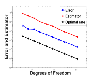
Refer to caption
Refer to caption
Figure 6.1. Error and Estimator for Example 1
Refer to caption
Refer to caption
Refer to caption
Figure 6.2. Efficiency Index, adaptive Mesh and discrete active set (yellow part) for Example 1

Example 2. To illustrate the efficacy of adaptive refinement, we consider this example with non-convex domain [7]. Therein, we have the following data

ΩΩ\displaystyle\Omega =(2,2)2[0,2)×(2,0],χ=0,formulae-sequenceabsentsuperscript2220220𝜒0\displaystyle=(-2,2)^{2}\setminus[0,2)\times(-2,0],\quad\chi=0,
u𝑢\displaystyle u =r2/3sin(2θ/3)γ1(r),absentsuperscript𝑟23𝑠𝑖𝑛2𝜃3subscript𝛾1𝑟\displaystyle=r^{2/3}sin(2\theta/3)\gamma_{1}(r),
f𝑓\displaystyle f =r2/3sin(2θ/3)(γ1(r)r+γ1′′(r))43r1/3sin(2θ/3)γ1(r)γ2(r)absentsuperscript𝑟23𝑠𝑖𝑛2𝜃3superscriptsubscript𝛾1𝑟𝑟superscriptsubscript𝛾1′′𝑟43superscript𝑟13𝑠𝑖𝑛2𝜃3superscriptsubscript𝛾1𝑟subscript𝛾2𝑟\displaystyle=-r^{2/3}sin(2\theta/3)\Big{(}\frac{\gamma_{1}^{{}^{\prime}}(r)}{r}+\gamma_{1}^{{}^{\prime\prime}}(r)\Big{)}-\frac{4}{3}r^{-1/3}sin(2\theta/3)\gamma_{1}^{{}^{\prime}}(r)-\gamma_{2}(r)
where
γ1(r)subscript𝛾1𝑟\displaystyle\gamma_{1}(r) ={1,r~<06r~5+15r~410r~3+1,0r~<10,r~1,absentcases1~𝑟0otherwise6superscript~𝑟515superscript~𝑟410superscript~𝑟310~𝑟1otherwise0~𝑟1otherwise\displaystyle=\begin{cases}1,\quad\tilde{r}<0\\ -6\tilde{r}^{5}+15\tilde{r}^{4}-10\tilde{r}^{3}+1,\quad 0\leq\tilde{r}<1\\ 0,\quad\tilde{r}\geq 1,\\ \end{cases}
γ2(r)subscript𝛾2𝑟\displaystyle\gamma_{2}(r) ={0,r541,otherwiseabsentcases0𝑟54otherwise1otherwiseotherwise\displaystyle=\begin{cases}0,\quad r\leq\frac{5}{4}\\ 1,\quad\mbox{otherwise}\end{cases}
withr~=2(r1/4).with~𝑟2𝑟14\displaystyle\text{with}\quad\tilde{r}=2(r-1/4).

The behavior of the true error and the error estimator for SIPG method is depicted in Figure 6.3. This figure ensures the optimal convergence (rate DOFs-1 ) of the error and the estimator together with the reliability of the estimator. The convergence behavior of single estimators ηi,i=1,2,3,4,6formulae-sequencesubscript𝜂𝑖𝑖12346\eta_{i},i=1,2,3,4,6 in maximum norm is also depicted in 6.3. The efficiency of the estimator is shown in Figure 6.4 (leftmost sub-figure). The adaptive mesh refinement and the discrete contact set at refinement level 26 are also reported in Figure 6.4. From these figures we observe that the estimator captures the singular behavior of the solution very well. The mesh refinement near the free boundary is higher because of the large jump in gradients.
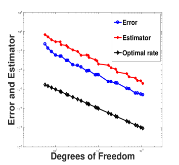
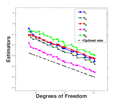
Refer to caption
Refer to caption
Figure 6.3. Error and Estimator for Example 2
Refer to caption
Refer to caption
Refer to caption
Figure 6.4. Efficiency Index, adaptive Mesh and discrete active set (yellow part) for Example 2

Example 3 In this example, we consider the following data from [40]:

ΩΩ\displaystyle\Omega =(2,2)×(1,1),r2=x2+y2,formulae-sequenceabsent2211superscript𝑟2superscript𝑥2superscript𝑦2\displaystyle=(-2,2)\times(-1,1),\quad r^{2}=x^{2}+y^{2},
χ𝜒\displaystyle\chi =106(x21)220(r2x2).absent106superscriptsuperscript𝑥21220superscript𝑟2superscript𝑥2\displaystyle=10-6(x^{2}-1)^{2}-20(r^{2}-x^{2}).

The exact solution is not known for this example. Figure 6.5 illustrate the behavior of the error estimator ηhsubscript𝜂\eta_{h} together with the individual estimators ηi,i=1,6formulae-sequencesubscript𝜂𝑖𝑖16\eta_{i},i=1,...6 for the load function f=0𝑓0f=0 and f=15𝑓15f=-15. We clearly observe that in both cases the estimator converges with optimal rate (DOFs-1). The adaptive mesh and discrete contact set at refinement level 13 for f=0𝑓0f=0 and f=15𝑓15f=-15 are shown in figures 6.6 and 6.7, respectively. The graph of the obstacle can be viewed as two hills connected by a saddle. As the load f𝑓f increases the change in the contact region can be observed from Figure 6.7 and as expected, we observe more refinement near the free boundaries.
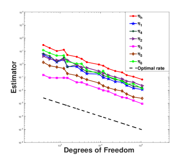
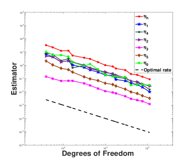
Refer to caption
Refer to caption
Figure 6.5. Estimator for Example 3 for f=0𝑓0f=0 and f=15𝑓15f=-15
Refer to caption
Refer to caption
Figure 6.6. Adaptive mesh for Example 3 for f=0𝑓0f=0 and f=15𝑓15f=-15
Refer to caption
Refer to caption
Figure 6.7. Discrete active set (yellow part) for Example 3 for f=0𝑓0f=0 and f=15𝑓15f=-15

References

  • [1] R. A. Adams, Sobolev spaces, Pure and Applied Mathematics, Academic Press, Inc., a subsidiary of Harcourt Brace Jovanovich, Publishers, New York-San Francisco-London, 1975.
  • [2] S. Agmon, Lectures on elliptic boundary value problems, D. Van Nostrand Co., Inc., Princeton, N.J.-Toronto-London, 1965.
  • [3] M. Ainsworth and J. T. Oden, A posteriori error estimation in finite element analysis, Pure and Applied Mathematics (New York). Wiley-Interscience [John Wiley & Sons], New York, 2000.
  • [4] C. Baiocchi, Estimation d’rreur dans Lsuperscript𝐿{L}^{\infty} pour les inéquations á obstacle, in mathematical aspects of finite element methods, Proc. Conf. Rome 1975, I. Galligani and E. Magenes, eds., Lect. Notes Math, Springer, Berlin 606 (1977), 27–34.
  • [5] S. Bartels and C. Carstensen, Averaging techniques yield reliable a posteriori finite element error control for obstacle problems, Numer. Math. 99 (2004), 225–249.
  • [6] D. Braess, A posteriori error estimators for obstacle problems-another look, Numer. Math. 101 (2005), 415–421.
  • [7] D. Braess, C. Carstensen, and R.H.W. Hoppe, Convergence analysis of a conforming adaptive finite element method for an obstacle problem, Numer. Math. 107 (2007), 455–471.
  • [8] F. Brezzi and L. A. Caffarelli, Convergence of the discrete free boundaries for finite element approximations, RAIRO Anal. Numer. 17 (1983), 385–395.
  • [9] F. Brezzi, W. W. Hager, and P. A. Raviart, Error estimates for the finite element solution of variational inequalities, Part I. primal theory, Numer. Math. 28 (1977), 431–443.
  • [10] F. Brezzi, W.W. Hager, and P.A. Raviart, Error estimates for the finite element solution of variational inequalities, Part. II: Mixed methods, Numer. Math. 31 (1978), 1–16.
  • [11] L. A. Caffarelli and D. Kinderlehrer, Potential methods in variational inequalities, J. Anal Math. 37 (1980), 285–295.
  • [12] E. Casas, Control of an elliptic problem with pointwise state constraints, SIAM J. Control and Optimization 24(6) (1986), 1309–1318.
  • [13] Z. Chen and R. Nochetto, Residual type a posteriori error estimates for elliptic obstacle problems, Numer. Math. 84 (2000), 527–548.
  • [14] P.G. Ciarlet, The finite element method for elliptic problems, North-Holland, Amsterdam, 1978.
  • [15] B. Ayuso de Dios, T. Gudi, and K. Porwal, A posteriori error estimates in maximum norm for interior penalty discontinuous Galerkin approximation of the obstacle problem, Domain decomposition methods in science and engineering XXVI, Lect. Notes Comput. Sci. Eng., (Springer, ed.), accepted.
  • [16] A. Demlow and E. H. Georgoulis, Pointwise a posteriori error control for discontinuous Galerkin methods for elliptic problems, SIAM J. Numer. Anal. 50 (2012), 2159–2181.
  • [17] A. Demlow and N. Kopteva, Maximum-norm a posteriori error estimates for singularly perturbed elliptic reaction-diffusion problems, Numer. Math. 133 (2016), no. 4, 707–742.
  • [18] H. Dong and S. Kim, Green’s matrices of second order elliptic systems with measurable coefficients in two dimensional domains, Trans. Amer. Math. Soc. 361 (2009), 3303–3323.
  • [19] R. S. Falk, Error estimates for the approximation of a class of variational inequalities, Math. Comp. 28 (1974), 963–971.
  • [20] F. Fierro and A. Veeser, A posteriori error estimators for regularized total variation of characteristic functions, SIAM J. Numer. Anal. 41 (2003), 2032–2055.
  • [21] J. Frehse, On the smoothness of variational inequalities with obstacle, Partial differential equations (Warsaw, 1978) (1983), 87–128.
  • [22] S. Gaddam and T. Gudi, Bubbles enriched quadratic finite element method for the 3d-elliptic obstacle problem, Comput. Meth. Appl. Math. 18 (2018), 223–236.
  • [23] by same author, Inhomogeneous dirichlet boundary condition in the a posteriori error control of the obstacle problem, Comput. Math. Appl. 75 (2018), 2311–2327.
  • [24] D. Gilbarg and N. S. Trudinger, Elliptic partial differential equations of second order, Springer-Verlag, Berlin, 2001.
  • [25] R. Glowinski, Numerical methods for nonlinear variational problems, Springer-Verlag, Berlin, 2008.
  • [26] M. Grüter and K.-O. Widman, The Green function for uniformly elliptic equations, Manuscr. Math. 37 (1982), no. 3, 303–342.
  • [27] T. Gudi and K. Porwal, A posteriori error control of discontinuous Galerkin methods for elliptic obstacle problems, Math. Comp. 83 (2014), 579–602.
  • [28] by same author, A remark on the a posteriori error analysis of discontinuous Galerkin methods for obstacle problem, Comput. Meth. Appl. Math. 14 (2014), 71–87.
  • [29] by same author, A reliable residual based a posteriori error estimator for quadratic finite element method for the elliptic obstacle problem, Comp. Meth. Appl. Math. 15 (2015), 145–160.
  • [30] M. Hintermüller, K. Ito, and K. Kunish, The primal-dual active set strategy as a semismooth Newton method, SIAM J. Optim. 13 (2003), 865–888.
  • [31] S. Hofmann and S. Kim, The Green function estimates for strongly elliptic systems of second order, Manuscr. Math. 24 (2007), 139–172.
  • [32] O.A. Karakashian and F. Pascal, A posteriori error estimates for a discontinuous Galerkin approximation of second-order elliptic problems, SIAM J. Numer. Anal. 41 (2003), 2374–2399.
  • [33] D. Kinderlehrer and G. Stampacchia, An introduction to variational inequalities and their applications, SIAM, Philadelphia, 2000.
  • [34] J. Nitsche, Lsuperscript𝐿{L}^{\infty} convergence of finite element approximations, in mathematical aspects of finite element methods, Proc. Conf. Rome 1975, I. Galligani and E. Magenes, eds., Lectures Notes Math 606 (1977), 261–274.
  • [35] R. Nochetto, T. V. Petersdorff, and C. S. Zhang, A posteriori error analysis for a class of integral equations and variational inequalities, Numer. Math. 116 (2010), 519–552.
  • [36] R. H. Nochetto, Pointwise a posteriori error estimates for elliptic problems on highly graded meshes, Math. Comp. 64 (1995), 1–22.
  • [37] R. H. Nochetto, E. Otárola, and A. J. Salgado, Convergence rates for the classical, thin and fractional elliptic obstacle problems, Philos. Trans. Roy. Soc. A 373 (2015), no. 2050, 20140449, 14.
  • [38] R.H. Nochetto, A. Schmidt, K.G. Siebert, and A. Veeser, Pointwise a posteriori error estimates for monotone semi-linear equations, Numer. Math. 104 (2006), 515–538.
  • [39] R.H. Nochetto, K.G. Siebert, and A. Veeser, Pointwise a posteriori error control for elliptic obstacle problems, Numer. Math. 95 (2003), 163–195.
  • [40] R.H. Nochetto, K.G. Siebert, and A. Veeser, Fully localized a posteriori error estimators and barrier sets for contact problems, SIAM J. Numer. Anal. 42(5) (2005), 2118–2135.
  • [41] G. Stampacchia, Le problème de Dirichlet pour les équations elliptiques du second ordre à coefficients discontinus, Annales de l’Institut Fourier 15 (1965), no. 1, 189–257.
  • [42] A. Veeser, Efficient and reliable a posteriori error estimators for elliptic obstacle problems, SIAM J. Numer. Anal. 39 (2001), 146–167.
  • [43] F. Wang, W. Han, and X. Cheng, Discontinuous Galerkin methods for solving elliptic variational inequalities, SIAM J. Numer. Anal. 48 (2010), 708–733.
  • [44] L. Wang, On the quadratic finite element approximation to the obstacle problem., Numer. Math. 92 (2002), 771–778.