Connections between galaxy properties and halo formation time in the cosmic web

Abstract

By linking galaxies in Sloan Digital Sky Survey (SDSS) to subhaloes in the ELUCID simulation, we investigate the relation between subhalo formation time and the galaxy properties, and the dependence of galaxy properties on the cosmic web environment. We find that central and satellite subhaloes have different formation time, where satellite subhaloes are older than central subhaloes at fixed mass. At fixed mass, the galaxy stellar-to-subhalo mass ratio is a good proxy of the subhalo formation time, and increases with the subhalo formation redshifts, especially for massive galaxies. The subhalo formation time is dependent on the cosmic web environment. For central subhaloes, there is a characteristic subhalo mass of $\sim 10^{12}\,h^{-1}{\rm M}_{\odot}$, below which subhaloes in knots are older than subhaloes of the same mass in filaments, sheets, or voids, while above which it reverses. The cosmic web environmental dependence of stellar-to-subhalo mass ratio is similar to that of the subhalo formation time. For centrals, there is a characteristic subhalo mass of $\sim 10^{12}\,h^{-1}{\rm M}_{\odot}$, below which the stellar-to-subhalo mass ratio is higher in knots than in filaments, sheets and voids, above which it reverses. Galaxies in knots have redder colors below $10^{12}\,h^{-1}{\rm M}_{\odot}$, while above $10^{12}\,h^{-1}{\rm M}_{\odot}$, the environmental dependence vanishes. Satellite fraction is strongly dependent on the cosmic web environment, and decreases from knots to filaments to sheets to voids, especially for low-mass galaxies.

1 Introduction

In the current standard $\Lambda$CDM model, galaxies are believed to form through baryonic gas cooling and condensation in dark matter haloes which reside in the context of cosmic web composed of knots, filaments, sheets and voids (White & Rees, 1978; Bond et al., 1996). Therefore, the properties of galaxies are expected to closely linked to their host haloes, as well as the large-scale environment (Lim et al., 2016; Correa & Schaye, 2020; Xu et al., 2020b). The physical connection among galaxies, haloes and the cosmic web environment is an interesting and challenging problem in the study of galaxy formation and evolution (Musso et al., 2018; Lange et al., 2019).

From cosmological $N$-body simulations, it’s well established that the clustering of haloes depends not only on the halo mass, but also other properties of dark matter haloes, such as the halo formation time. This is so called halo assembly bias (Sheth & Tormen, 2004; Gao et al., 2005; Wechsler et al., 2006; Gao & White, 2007; Zentner et al., 2014; Contreras et al., 2019; Mansfield & Kravtsov, 2020). Using $N$-body simulation, Gao et al. (2005) showed that the clustering of haloes are strongly dependent on the halo formation time. For haloes at low-mass end, older haloes cluster more strongly than younger haloes of the same mass. For haloes at high-mass end, Jing et al. (2007) found that the age dependence is reversed, where older haloes are less clustered than younger haloes of the same mass. The dependence of halo clustering on halo formation time besides mass is also extended to other halo properties, such as concentration, spin, shape (Wechsler et al., 2006; Lacerna & Padilla, 2012; Villarreal et al., 2017).

In observation, there is no consensus on a robust determination of the assembly bias in the galaxy distribution, referred to as galaxy assembly bias. Although some studies claimed that the assembly bias in galaxy distribution is significantly robust (Yang et al., 2006; Cooper et al., 2010; Wang et al., 2013; Lacerna et al., 2014; Miyatake et al., 2016; Ferreras et al., 2019; Obuljen et al., 2020; Yuan et al., 2020), others argued that the galaxy assembly bias signal is small or negligible and may be a result of the systematic uncertainties (Blanton & Berlind, 2007; Tinker et al., 2008; Lin et al., 2016; Zu & Mandelbaum, 2016; Dvornik et al., 2017; Zu et al., 2017; Tinker et al., 2017, 2018; Salcedo et al., 2020). Assuming that redder galaxies live in older haloes, Hearin & Watson (2013) developed an age-matching model by extending the traditional abundance-matching technique. In the age-matching model, the galaxy colour at fixed luminosity is assumed to be monotonically correlated with the halo age at fixed $V_{\rm max}$, which is the halo maximum circular velocity. Hearin et al. (2014) claimed that the age-matching model can accurately predict colour-dependent galaxy clustering and a variety of galaxy group statistics. In contrast, Zu & Mandelbaum (2016) found that the age-matching model fails to reproduce the observed halo mass for massive blue centrals, using the galaxy-galaxy lensing measurements split by colour in bins of galaxy stellar mass. Tinker et al. (2017) claimed that the measurements of the quenched fraction of centrals can not be reconciled with the prediction of the age-matching model for low-mass galaxies, implying that there is no relation between halo formation time and galaxy quenching for centrals.

In some previous studies (Yang et al., 2006; Wang et al., 2013; Hearin & Watson, 2013; Hearin et al., 2014; Watson et al., 2015), one key assumption is that the galaxy color or specific star formation rate is a good indicator of halo formation time. However, Lin et al. (2016) found no convincing evidence of galaxy assembly bias using specific star formation rate as a proxy of halo formation time, which indicates that the galaxy sSFR is not well correlated with the halo formation history. Because of the inconsistent studies of galaxy assembly bias in observation, one of the purposes in this work is to find which galaxy property is tightly correlated with the halo formation time.

In this work, with the help of the constrained ELUCID simulation, the properties of ture galaxies in observation can be related with the formation time of dark matter subhaloes in simulation, so that we can directly check which property is the best proxy of halo formation time. Using the ELUCID simulation, galaxies in observation can be linked to dark matter subhaloes in simulation using a neighborhood abundance matching method (Yang et al., 2018), since the mass and positions of haloes at $z\sim 0$ in ELUCID simulation are consistent with those of galaxy groups in observation, due to the initial condition of the ELUCID simulation constrained from the density field of galaxy distribution in observation (Wang et al., 2012; Wang et al., 2014, 2016; Zhang et al., 2021).

Besides, in order to interpret galaxy or halo assembly bias, recent studies have focused on the key role of the cosmic web environment (Tojeiro et al., 2017; Yang et al., 2017; Musso et al., 2018; Sinigaglia et al., 2020), and claimed that the tidal anisotropy of cosmic web environment is the primary indicator of halo assembly bias (Paranjape et al., 2018a, b; Ramakrishnan et al., 2019; Xu et al., 2020a; Ramakrishnan & Paranjape, 2020). Therefore, to better understand the assembly bias, recent studies have focused on the influence of cosmic web environment on the galaxy or halo properties (Hahn et al., 2007a; Wang et al., 2011; Chen et al., 2020; Xu et al., 2020b).

On the one hand, there are lots of evidence that the cosmic web environment affects galaxy or halo properties (Chen et al., 2017; Kraljic et al., 2018). Using a series of $N$-body simulations, Hahn et al. (2007a) claimed that for low-mass haloes, the formation redshifts strongly depend on the cosmic web environment, and haloes of fixed mass tend to be older in knots and younger in voids. Using data from the Galaxy And Mass Assembly (GAMA) survey, Alpaslan et al. (2016) found that galaxies closer to the cylindrical axes of the filaments have lower specific star formation rate at a given mass. Using galaxies from SDSS DR 12, Chen et al. (2017) claimed that at a given stellar mass, older galaxies tend to reside closer to the cylindrical axes of the filaments than younger galaxies. Similar results have also been obtained in observation or hydrodynamical simulation (Malavasi et al., 2017; Laigle et al., 2018; Mahajan et al., 2018; Luber et al., 2019; Singh et al., 2020).

On the other hand, lots of studies supported that properties of galaxies or haloes are independent of their cosmic web location (geometric environment), but entirely determined by the environmental density (Alonso et al., 2015, 2016; Eardley et al., 2015; Brouwer et al., 2016; Goh et al., 2019). In simulation, Alonso et al. (2015) showed that the halo mass function depends only on their local environmental density, and not on the cosmic web location. In observation, using data from GAMA survey, Eardley et al. (2015) also claimed that the galaxy luminosity function is independent on the cosmic web location at the same environmental density. Using the Bolshoi-Planck simulation, Goh et al. (2019) claimed that at the same environmental density, there is no discernible difference between the halo properties (e.g. halo spin parameter, concentration, and specific mass accretion rate) in different cosmic web environment of filaments, walls, and voids. In addition, Alpaslan et al. (2015) claimed that the most important parameter driving galaxy properties is the stellar mass, as opposed to the cosmic web environment.

Interestingly, using galaxy groups in GAMA survey, Tojeiro et al. (2017) found that low-mass haloes show a steadily increasing galaxy stellar-to-halo mass ratio from voids to knots, with the trend be reversed at large halo mass (see also Xu et al., 2020b). This behavior indicates that at low-mass end, haloes in knots are older than haloes of the same mass in voids, if stellar-to-halo mass ratio is a good proxy of the halo formation time. Using galaxy groups from SDSS DR7, Lim et al. (2016) found that galaxy color is tightly correlated with stellar-to-halo mass ratio for low-mass central galaxies, and claimed that the ratio can be used as a proxy of the halo formation time.

In this work, combining galaxies in SDSS DR7 and subhaloes in the ELUCID simulation, we mainly focus on the relation between subhalo formation time and the stellar-to-subhalo mass ratio. In addition, we investigate the dependence of galaxy properties and subhalo formation time on the cosmic web environment.

This paper is organized as follows. In Section 2, we describe the subhalo catalog from the ELUCID simulation, and the observational data from SDSS DR7. In addition, we describe the novel neighborhood subhalo abundance matching method linking galaxies in observation to subhaloes in constrained simulation, and the cosmic web classification method. In Section 3, we investigate the relation between subhalo formation time and the galaxy properties. In Section 4, we study the dependence of galaxy properties on the cosmic web environment. Finally, we summarize our results in Section 5. Throughout this paper, the cosmological parameters are $\Omega_{m}=0.258$, $\Omega_{b}=0.044$, $\Omega_{\Lambda}=0.742$, $h=0.72$, $n_{s}=0.963$ and $\sigma_{8}=0.796$.

2 Data and methods

2.1 Subhaloes from ELUCID simulation

The ELUCID simulation is a dark matter only, constrained simulation, which can reproduce the density field of the nearby universe generated from the galaxy distribution in the SDSS observation. Therefore, the statistical properties of cosmic web are accurately reproduced in the ELUCID simulation, compared with the SDSS observation (Wang et al., 2016).

The initial condition of the simulation is sampled with $3072^{3}$ dark matter particles at redshift $z=100$ in a periodic box of $500\,h^{-1}{\rm Mpc}$ on a side. The density field is then evolved to the present epoch with a memory-optimized version of GADGET2 (Springel, 2005) in the Center for High Performance Computing, Shanghai Jiao Tong University. In the simulation, $100$ snapshots are produced from redshift $z=18.4$ to $z=0$ with the expansion factor spaced in logarithmic space. The mass of each dark matter particle is $3.0875\times 10^{8}\,h^{-1}{\rm M}_{\odot}$. The ELUCID simulation adopts the cosmological parameters: $\Omega_{m}=0.258$, $\Omega_{b}=0.044$, $\Omega_{\Lambda}=0.742$, $h=0.72$, $n_{s}=0.963$ and $\sigma_{8}=0.796$.

From the simulation, the standard friends-of-friends (FOF) algorithm (Davis et al., 1985) is performed on the particle data to generate FOF haloes with a linking length of $b=0.2$ times the mean particle separation. Next, the SUBFIND algorithm (Springel et al., 2001) decomposes a given FOF halo into a set of disjoint, gravitationally bound substructures in the unbinding procedure, in which the gravitational potentials are iteratively calculated to remove the unbound particles in the host FOF halo (Springel et al., 2020). Within these substructures, the most massive one is called central subhalo, while the others are referred to satellite subhaloes. Compared with FOF haloes, a set of gravitationally bound subhaloes in simulation are more suitable to link central and satellite galaxies in observation. Therefore, in the following analysis, central subhaloes in simulation are linked to central galaxies in observation, while satellite subhaloes are matched to satellite galaxies (Yang et al., 2018).

For each central or satellite subhalo, the center of the subhalo is defined as the position of the most bound particle, which refers to the minimum binding energy particle. For two subhaloes $H_{a}$ and $H_{b}$ at subsequent redshift $z_{a}$ and $z_{b}$ $(z_{a}>z_{b})$, $H_{a}$ is defined as the progenitor of $H_{b}$ , if at least half of the particles of $H_{a}$ are contained in $H_{b}$ , and the most bound particle of $H_{a}$ is also contained in $H_{b}$. Note that according to this definition, in the constructed merger trees each subhalo can have several progenitors, but has only one descendant. From snapshot to snapshot, the most massive progenitors construct the main branch history of the merger trees, which can be used to calculate the formation times of the current subhaloes at $z=0$.

In order to obtain more reliable formation time of the subhalo from the merger trees in ELUCID simulation, in the following analysis, we only focus on subhaloes at $z=0$ with mass larger than $10^{10.5}\,h^{-1}{\rm M}_{\odot}$ containing at least $100$ dark matter particles.

2.2 Galaxies from SDSS DR7

The galaxy sample used in this paper is from the SDSS (York et al., 2000), which is one of the most successful surveys in the history of astronomy. Based on the multi-band imaging and spectroscopic survey SDSS DR7 (Abazajian et al., 2009), Blanton et al. (2005) constructed the New York University Value-Added Galaxy Catalog (NYU-VAGC) with an independent set of improved reductions. From the NYU-VAGC, we collect a total of $639,359$ galaxies with redshifts in the range $0.01\leq z\leq 0.2$, with redshift completeness ${\cal C}_{z}>0.7$, and with extinction-corrected apparent magnitude brighter than $r\leq 17.72$.

The absolute magnitudes of galaxies are calculated and K-corrected and evolution corrected to $z=0.1$ (Yang et al., 2007), using the method described by Blanton et al. (2003) and Blanton & Roweis (2007). The stellar masses and star formation rates of galaxies are from the public catalog of Chang et al. (2015) with reliable aperture corrections. Besides, we have checked our results using the stellar mass computed by the relation between stellar mass-to-light ratio and the color of Bell et al. (2003, see also () for details). We found that the final results are not sensitive to the different stellar mass used. Throughout this paper, the stellar masses from Chang et al. (2015) are used unless stated otherwise.

A total of $639,359$ galaxies have a sky coverage of $7,748$ square degree, consisting of two parts: a large continuous region in the Northern Galactic Cap (NGC) and a small region in the Southern Galactic Cap. Since the initial condition of the constrained ELUCID simulation is constructed from the distribution of the galaxies in the continuous NGC region, in the following analysis, we only select galaxies located in the range $99^{\circ}<\alpha<283^{\circ}$ and $-7^{\circ}<\delta<75^{\circ}$, resulting in a total of 396, 069 galaxies in the continuous NGC region. Here $\alpha$ and $\delta$ are the right ascension and declination, respectively.

2.3 Linking galaxies in observation to subhaloes in simulation

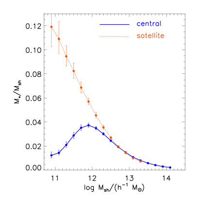
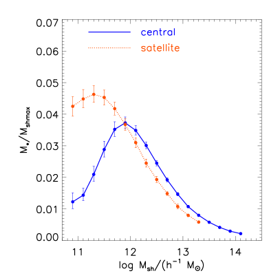
Figure 1: The ratio of galaxy stellar mass relative to the current (left panel) and maximum (right panel) subhalo mass as a function of the subhalo mass. The blue solid and red dashed lines show the median values for central and satellite galaxies, respectively. The error bars show the $45$ per cent and $55$ per cent quantiles.

In the constrained ELUCID simulation, the spatial distributions of the subhaloes at present are tightly correlated with the distributions of galaxies in SDSS DR7 (Wang et al., 2016; Yang et al., 2018), because the simulation makes use of the initial condition constrained by the mass density field extracted from the distribution of galaxies in SDSS DR7.

Galaxies in observation are linked to dark matter subhaloes in the ELUCID simulation using a neighborhood abundance matching method (Yang et al., 2018). For each galaxy in observation, we search for its corresponding subhalo in simulation according to the likelihood

$$P=M_{\rm shmax}\exp\left(-\frac{r_{p}^{2}}{2r_{\rm off}^{2}}\right)\exp\left(-\frac{\pi^{2}}{2v_{\rm off}^{2}}\right),$$ (1)

where $r_{p}$ and $\pi$ are the separations in the redshift space between the galaxy and the subhalo in the perpendicular and parallel to the line-of-sight directions, respectively. $r_{\rm off}$ and $v_{\rm off}$ are two free parameters, while $M_{\rm shmax}$ is the peak mass of the subhalo under consideration. For $r_{\rm off}$ and $v_{\rm off}$ , the parameters are set to be $r_{\rm off}=5\,h^{-1}{\rm Mpc}$ and $v_{\rm off}=1000\leavevmode\nobreak\ {\rm km/s}$, which can give better constraint for the stellar-to-subhalo mass relation, especially for the low-mass subhaloes. Note that in Equation 1, the mass $M_{\rm shmax}$ is the dominant variable in the neighborhood abundance matching method, which will degrade to the traditional abundance matching method if $r_{\rm off}=\infty$ and $v_{\rm off}=\infty$ in the extreme case.

Generally, the subhalo abundance matching models populate subhaloes with galaxies base on the peak values of the mass or the circular velocity over the merger histories of the subhaloes (Conroy et al., 2006; Moster et al., 2010; Reddick et al., 2013; Matthee et al., 2017; Campbell et al., 2018; van den Bosch & Ogiya, 2018), since the maximum values are found to be better correlated with the galaxy clustering statistics than the current values at redshift $z=0$. The current and peak values of the subhaloes are different in the accretion history, especially for satellite subhaloes. In the accretion and merger history, satellite subhaloes are commonly subject to tidal stripping in a larger system and remove dark matter mass, while the stellar components in the core are more tightly bound than dark matter and change the stellar masses slightly. Therefore, the peak values are better tracers of the potential well that shapes the galaxy statistical properties.

In the neighborhood abundance matching method, we use the peak mass of the subhaloes to link central subhaloes in simulation to central galaxies in observation, and satellite subhaloes to satellite galaxies, respectively. From the galaxy-subhalo connection catalog, Figure 1 shows the ratios of galaxy stellar mass $M_{*}$ to the current $M_{\rm sh}$ and peak $M_{\rm shmax}$ subhalo mass for central and satellite galaxies, respectively. Here the galaxy stellar mass is estimated from Chang et al. (2015), and the subhalo mass is obtained from the matched subhalo in ELUCID simulation using the neighborhood abundance matching method.

Figure 1 shows that central and satellite galaxies have different stellar-to-subhalo mass ratios $M_{*}/M_{\rm sh}$ at fixed subhalo mass, especially for galaxies in low-mass subhaloes. This is due to the different formation and evolution histories between central and satellite galaxies. Satellite subhaloes commonly lose their mass due to tidal stripping after accretion into a larger system, while the concentrated stellar components change their mass slightly in the core of the subhalo. This behavior can be also indicated by comparing the red dashed lines between the left and right panels. For satellites at fixed subhalo mass, the ratio $M_{*}/M_{\rm sh}$ is significantly larger than the ratio $M_{*}/M_{\rm shmax}$, especially for the low-mass satellite subhaloes, which indicates that satellite galaxies in low-mass subhaloes lose their dark matter mass significantly.

However, for centrals, the blue solid lines in left and right panels show that the ratios $M_{*}/M_{\rm sh}$ and $M_{*}/M_{\rm shmax}$ at fixed subhalo mass have almost no difference, since for centrals the maximum mass $M_{\rm shmax}$ is almost the same as the current mass $M_{\rm sh}$ at $z=0$.

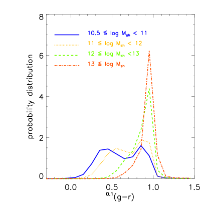
Figure 2: Probability distribution function of the colors of the galaxies within subhaloes in different mass ranges, which are indicated by different type lines in the figure.

Given each galaxy in observation is now linked with a subhalo in the ELUCID simulation, we show in Figure 2 the probability distribution of the colors ${}^{0.1}(g-r)$ of galaxies within the fixed subhalo mass bins. In the galaxy-subhalo connection catalog, there are $42,431$, $236,836$, $87,541$ and $9,813$ galaxies with their corresponding subhalo mass $\log(M_{\rm sh}/(\,h^{-1}{\rm M}_{\odot}))$ in the ranges of $(10.5,11)$, $(11,12)$, $(12,13)$, and $(13,\infty)$, which are indicated by different type lines in Figure 2. Obviously, the galaxies in the subhaloes with $\log(M_{\rm sh}/(\,h^{-1}{\rm M}_{\odot}))$ mass in the ranges $(10.5,11)$ and $(11,12)$ have the bimodal distribution in the ${}^{0.1}(g-r)$ color. This behavior is similar to the bimodal distribution of galaxy colors at fixed absolute magnitude (Baldry et al., 2004).

2.4 subhalo formation time and environment

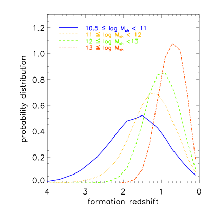
Figure 3: Probability distribution function of the formation redshifts of subhaloes in different mass ranges.

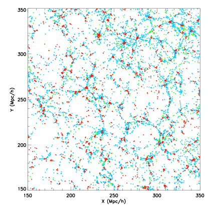
Figure 4: Spatial distribution of subhaloes in different environments in a slice of thickness $10\,h^{-1}{\rm Mpc}$. Only dark matter subhaloes linked to galaxies in SDSS DR7 are shown. The symbol sizes of the subhaloes are proportional to their radii. The subhaloes in four different environments are indicated by different colors: knot(red), filament(cyan), sheet(green) and void(blue).

Based on subhaloes identified by the algorithm SUBFIND, merger trees are constructed by linking a subhalo in one snapshot to a single descendant subhalo in the subsequent snapshot. Therefore, the halo merger tree is indeed a subhalo merger tree in this study (Springel et al., 2005). The formation time of the subhalo is defined as the time at which the main branch progenitor reached half of its maximum mass $M_{\rm shmax}$.

Figure 3 shows the probability distribution of the formation redshift of the subhaloes in different mass ranges, which are indicated by different type lines in the figure. Here again, we separate the total of $396,069$ subhaloes in the galaxy-subhalo pairs into four subsamples according to their mass with $\log(M_{\rm sh}/(\,h^{-1}{\rm M}_{\odot}))$ in the ranges $(10.5,11)$, $(11,12)$, $(12,13)$, and $(13,\infty)$. For $236,836$ subhaloes in the mass range $10^{11}\,h^{-1}{\rm M}_{\odot}\leq M_{\rm sh}<10^{12}\,h^{-1}{\rm M}_{\odot}$, about $68\%$ subhaloes have their formation time in the redshift range $0.65\leq z\leq 1.75$.

The geometric environment in which the subhalo (galaxy) resides is classified into knot, filament, sheet, and void  by the Hessian matrix of the smoothing density field (Zhang et al., 2009)

$$H_{ij}({\boldsymbol{x}})=\frac{\partial^{2}\rho_{s}({\boldsymbol{x}})}{\partial x_{i}\partial x_{j}},$$ (2)

where $i$ and $j$ are the Hessian matrix indices with values of $1$, $2$ or $3$. The smoothing density field $\rho_{s}$ is calculated by the Gaussian filter with a fixed smoothing scale $R_{s}=2.1\,h^{-1}{\rm Mpc}$ (Aragón-Calvo et al., 2007; Hahn et al., 2007b; Zhang et al., 2009). The eigenvalues of the Hessian matrix $H_{ij}$ are calculated at the position $\boldsymbol{x}$ of each subhalo. According to the number of negative eigenvalues, the subhalo’s environment is classified into one of four cosmic web types. If all of the three eigenvalues are negative, the subhalo’s environment is classified into knot, while the case of two, one or zero negative eigenvalue corresponds to filament, sheet or void, respectively (Zhang et al., 2009).

Of the $396,069$ subhaloes (galaxies) in galaxy-subhalo connection catalog, $148,055$ $(37.4\%)$ are located in knot, $217,746$ $(55.0\%)$ are located in filament, $29,909$ $(7.6\%)$ are located in sheet and $359$ $(0.09\%)$ are located in void. Figure 4 shows the spatial distribution of subhaloes in a $200\,h^{-1}{\rm Mpc}\times 200\,h^{-1}{\rm Mpc}$ slice of thickness $10\,h^{-1}{\rm Mpc}$. Note that only subhaloes linked to galaxies in SDSS DR7 are shown in Figure 4. The subhaloes in four different environments are indicated by different colors: knot(red), filament(cyan), sheet(green) and void(blue).

3 Proxy of halo formation time

In this section, we investigate how the galaxy properties are correlated with subhalo formation time, using the catalog of galaxies linked to the subhaloes in the ELUCID simulation. To find a reasonable proxy of subhalo formation time, we mainly focus on the ratio of stellar mass to subhalo mass. In most of our subsequent probes, we separate central or satellite galaxies into four subsamples with their corresponding subhalo mass $\log(M_{\rm sh}/(\,h^{-1}{\rm M}_{\odot}))$ in the ranges of $(10.5,11)$, $(11,12)$, $(12,13)$, and $(13,\infty)$.

3.1 formation redshifts for central and satellite subhaloes

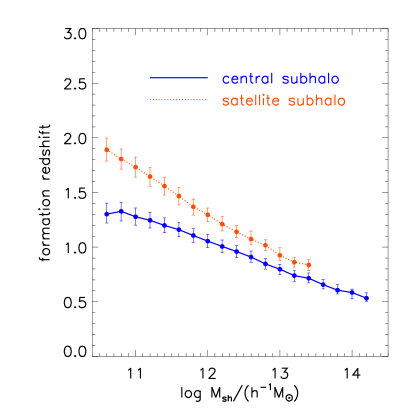
Figure 5: Subhalo formation redshifts as a function of the mass of central and satellite subhaloes. The blue solid and red dashed lines show the median values for central and satellite subhaloes, respectively.

In simulation, we define central subhalo to be the most massive subhalo in a given host FOF halo, and satellite subhaloes to be any other subhaloes. Based on the subhalo merger trees from ELUCID simulation, the formation time of the subhalo is defined as the redshift at which the main branch progenitor reached half of its maximum mass $M_{\rm shmax}$. To obtain a reliable measurement of the subhalo formation time, we mainly focus on the subhaloes containing at least $100$ dark matter particles with mass larger than $10^{10.5}\,h^{-1}{\rm M}_{\odot}$.

In the evolutionary process from high redshift to the present, the mass of central subhalo generally grows larger and larger across the main branch of the merger trees, while satellite subhaloes usually lose their mass on account of tidal stripping or dynamical friction in the process of accretion into the host haloes (van den Bosch & Ogiya, 2018; Rodriguez et al., 2020). Therefore, the distinct assembly histories of central and satellite subhaloes result in different subhalo formation time for central and satellite subhaloes. Figure 5 shows the median values of the formation redshifts of central and satellite subhaloes as a function the subhalo mass. Obviously, at fixed subhalo mass, the formation redshifts of satellite subhaloes are larger than those of central subhaloes.

Therefore, in the following analysis, we investigate the properties of central and satellite subhaloes separately, due to the distinct assembly history of central and satellite subhaloes.

3.2 galaxy stellar-to-subhalo mass ratio

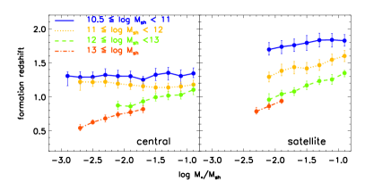
Figure 6: Subhalo formation redshift as a function of the stellar-to-subhalo mass ratio for central and satellite galaxies in different subhalo mass ranges.

The galaxy stellar-to-halo mass relation has been extensively studied using various techniques, such as the measurements of galaxy-galaxy lensing (Mandelbaum et al., 2016), satellite kinematics (Lange et al., 2019), and abundance matching model (Chaves-Montero et al., 2016; Dragomir et al., 2018; Contreras et al., 2020).

With the help of the constrained ELUCID simulation, we can directly make a one-to-one comparison between galaxy stellar-to-subhalo mass ratio and the formation time of the subhalo in simulation. Using the neighborhood subhalo abundance matching method to the constrained simulation, galaxies in observation are linked to subhaloes in ELUCID simulation, according to not only their mass, but also their positions. Therefore, the galaxy-subhalo connection catalog used in this paper is more reliable than that generated by traditional abundance matching model.

Figure 6 shows the formation time of the subhalo as a function of galaxy stellar-to-subhalo mass ratio $M_{*}/M_{\rm sh}$ for central and satellite galaxies. As shown in the left panel of Figure 6, the subhalo formation redshifts increase with the stellar-to-subhalo mass ratios for central galaxies in subhaloes with $M_{\rm sh}\geq 10^{12}\,h^{-1}{\rm M}_{\odot}$, while for central galaxies with subhalo mass $M_{\rm sh}<10^{12}\,h^{-1}{\rm M}_{\odot}$, the formation time of the subhalo seems to be independent on galaxy stellar-to-subhalo mass ratio. The flat trend blue and orange lines in the left panel of Figure 6 may be because the matched galaxy-subhalo pairs are dominated by Poisson errors (Tweed et al., 2017) and less reliable for low-mass subhaloes. As we have checked the mass ratios of the second to most massive subhaloes around the central galaxies, the ratio for subhaloes with mass $<10^{12}h^{-1}M_{\odot}$ is at $\ga 0.8$ level. Because of the scatter in the stellar-subhalo mass relation, it is not necessary that the most massive subhaloes give the best match with the central galaxies for these low mass subhaloes. While for those subhaloes with mass $\ga 10^{12}h^{-1}M_{\odot}$, the match should be much more reliable. In addition to this, in galaxy-subhalo pairs, there are a fraction of matched pairs with very large separations (see Figure. 2 in Yang et al., 2018), and the median projected and line-of-sight separations are $r_{p}=2.6\,h^{-1}{\rm Mpc}$ and $\pi=3.3\,h^{-1}{\rm Mpc}$, respectively. To check the impact of this, we have also generated several closely-matched subsamples with smaller separation $r_{p}$ and $\pi$, and performed similar measurements of Figure 6. We find that the trends of closely-matched subsamples keep almost unchanged compared with the current results.

In addition, we investigate the formation time of satellite galaxies as a function of galaxy stellar-to-subhalo mass ratio. For satellites galaxies as shown in the right panel of Figure 6, the subhalo formation redshifts also increase with the stellar-to-subhalo mass ratio.

Note that the initial condition of the constrained simulation is constructed using the galaxy groups with mass larger than $10^{12}\,h^{-1}{\rm M}_{\odot}$, thus the galaxy-subhalo pairs with subhalo mass larger than $10^{12}\,h^{-1}{\rm M}_{\odot}$ are more reliable in this study. In a word, the galaxy stellar-to-subhalo mass ratio is a good proxy of the formation time, especially for galaxies in high-mass subhaloes.

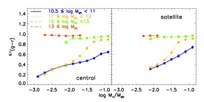
Figure 7: Galaxy colors as a function of the stellar-to-subhalo mass ratio for central and satellite galaxies. The solid points with different types of lines show the median values for galaxies in different subhalo mass ranges.

3.3 galaxy color

Using N-body simulations, Wang et al. (2011) investigated the correlations among different halo properties, and found that the mass ratio between the most massive subhalo and its host FOF halo is tightly correlated with the halo formation time, spin and shape. Inspired by this, Lim et al. (2016) investigated the correlation between galaxy stellar-to-halo mass ratio and galaxy properties, using galaxy groups selected by the halo-based group finder (Yang et al., 2007) from SDSS DR7. They found that galaxy stellar-to-halo mass ratio is tightly correlated with galaxy colors and star formation in observation.

Using the 396,069 galaxy-subhalo pairs, here we check the relation between the galaxy stellar-to-subhalo mass ratio and galaxy colors. Figure 7 shows the median values of galaxy colors as a function of the ratio of galaxy stellar-to-subhalo mass for central and satellite galaxies in different subhalo mass ranges, indicated by different types of lines in the figure. For galaxies in subhaloes with mass less than $10^{12}\,h^{-1}{\rm M}_{\odot}$, the galaxy stellar-to-subhalo mass ratio is tightly correlated with the galaxy colors, where redder galaxies have higher stellar-to-subhalo mass ratios. Note that, for a given subhalo mass, the galaxy stellar-to-subhalo mass ratio is proportional to the galaxy stellar mass. In general, the color dependence seen here might be attributed mainly by the stellar mass-color dependence. Only using observational data, Lim et al. (2016) also found that redder galaxies have higher stellar-to-group mass ratios, where the groups are selected by the halo-based group finder (Yang et al., 2007). In this study, using closely-matched subsamples with smaller separation $r_{p}$ and $\pi$, we have confirmed the color dependence of galaxy stellar-to-subhalo mass ratio for galaxies in low-mass subhaloes. The blue and orange lines in Figure 7 show that lower stellar-to-subhalo mass ratio galaxies are bluer, which seems to indicate that their star formation started later. Although because of the potential mismatches between low mass subhaloes and central galaxies, where the correlation between the subhalo formation time and the stellar-to-subhalo mass ratio can not be well recovered, the satellite galaxies do indicate that the galaxy colors are correlated with the subhalo formation time.

For galaxies in more massive subhaloes with mass larger than $10^{12}\,h^{-1}{\rm M}_{\odot}$, there is almost no dependence of galaxy colors on the stellar-to-subhalo mass ratio, because galaxies are all equally red in the high mass range.

4 Dependence on the cosmic web

The cosmic web environment in which the subhalo (galaxy) resides is classified into konts, filaments, sheets, and voids by the Hessian matrix of the smoothing density field (Zhang et al., 2009). Based on the geometric cosmic web classification, we investigate the dependence of subhalo formation time and galaxy properties on the cosmic web environment, using the catalog of galaxies in observation and subhaloes in ELUCID simulation.

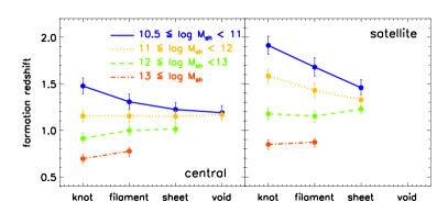
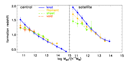
Figure 8: Subhalo formation redshift as a function of the cosmic web environment (top panels) and the subhalo mass (low panels) for central and satellite subhaloes. For satellite subhaloes in the right panels, there are no data points in the void, because there are almost no satellite subhaloes in the void  in our sample.

4.1 subhalo formation time

Using subhaloes from the ELUCID simulation, we investigate the dependence of the subhalo formation time on the cosmic web environment. The formation redshift of the subhalo is defined as the redshift at which the main branch progenitor reached half of its maximum mass $M_{\rm shmax}$.

In the top panels of Figure 8, we show the subhalo formation redshifts as a function of the cosmic web environment for central and satellite subhaloes in different mass range. For central subhaloes, in the low-mass range $(10.5,11)$, subhaloes in knots are older than subhaloes of the same mass in filaments, sheets or voids, while in the high-mass range $(12,13)$ and $(13,\infty)$, subhaloes in knots are younger than haloes of the same mass in sheets or filaments. For clarity, the low panels of Figure 8 shows the subhalo formation redshifts as a function of the subhalo mass in different cosmic environments. For central subhaloes, there is a characteristic subhalo mass of $10^{11.7}\,h^{-1}{\rm M}_{\odot}$, below which the formation redshifts are larger in knots than filaments, sheets or voids, while above which it reverses. For central subhaloes at high mass, the formation redshifts are smaller in knots.

As shown in the right panels in Figure 8, for satellite subhaloes below $10^{12.5}\,h^{-1}{\rm M}_{\odot}$, subhaloes in knots are older than subhaloes of the same mass in filaments or sheets. Above $10^{12.5}\,h^{-1}{\rm M}_{\odot}$, there are only $2$ satellite subhaloes in sheets and no satellite subhaloes in voids. Thus, the results are not robust for satellite subhaloes in high-mass range.

Actually, here the environmental dependence of the subhalo formation time is independent of the matching method, because the subhalo formation time, subhalo mass and cosmic web classifications used in Figure 8 are all from the simulation data. We have confirmed that similar results are obtained for a total of subhaloes including unmatched pairs in the ELUCID simulation. The environmental dependence of the halo formation time below or above the characteristic subhalo mass of $\sim 10^{12}\,h^{-1}{\rm M}_{\odot}$ that we have found is consistent with the analysis of halo assembly bias. For low-mass haloes, older haloes cluster more strongly than younger haloes (Gao et al., 2005; Gao & White, 2007), while for high-mass haloes, the trend is reversed, where older haloes are less clustered (Jing et al., 2007). One explanation is that for low-mass haloes in the knots environment, they are relatively located in the vicinity of clusters (Hahn et al., 2007a, b), and their mass accretions are suppressed by the hot environments produced by the tidal fields of clusters (Wang et al., 2007), resulting in the older ages of low-mass haloes in knots. However, for high-mass haloes, the heating of the large-scale tidal field is less important, and haloes in knots grows more easily by continuous accretion and major mergers.

To check if the above found features are robust with respect to our construction of the cosmic web, we perform our analysis for cosmic web constructed with additional two choices of smoothing scales $R_{s}=4.2$ and $8.4\,h^{-1}{\rm Mpc}$. We find that the transition characteristic subhalo mass for central subhalos slightly increases with the increase of the smoothing scale we used, as there are relatively more massive subhaloes classified into void regions. Nevertheless, the overall trends are very similar.

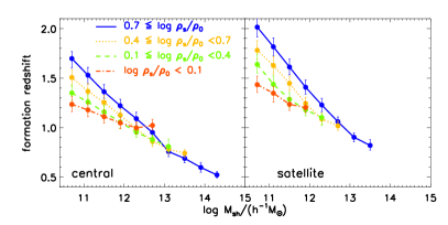
Figure 9: Subhalo fromation redshift as a function of the subhalo mass for central and satellite subhaloes in different cosmic density ranges of $\log\rho_{s}/\rho_{0}$, where $\rho_{s}$ is the smoothing density with Gaussian filter of $R_{s}=2.1\,h^{-1}{\rm Mpc}$ at the location of a given subhalo, and $\rho_{0}$ is the mean cosmic density of the universe.

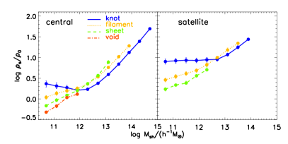
Figure 10: Cosmic density field as a function of the subhalo mass in different cosmic web environments for central and satellite subhaloes.

Figure 11: Similar to the low panels of Figure 8, but for subhaloes in the cosmic density range of $0.6<\log\rho_{s}/\rho_{0}<0.7$.

In order to further understand the environmental dependence of the subhalo formation time, we also investigate the effects of the local environmental density on the subhalo formation time. At the location of a given subhalo, the smoothing density field $\rho_{s}$ is calculated by smoothing the cloud-in-cell (CIC) generated density field with a spherically symmetric Gaussian filter of $R_{s}=2.1\,h^{-1}{\rm Mpc}$ (Zhang et al., 2009). Then we separate central or satellite subhaloes into four equal subsamples with their local environmental density $\log\rho_{s}/\rho_{0}$ in the ranges of $(-0.8,0.1)$, $(0.1,0.4)$, $(0.4,0.7)$, and $(0.7,2.0)$, where $\rho_{0}$ is the average cosmic matter density of the universe. Figure 9 shows the subhalo fromation redshift as a function of the subhalo mass for central and satellite subhaloes in different environmental density. For centrals or satellites, subhaloes in higher density are older than those in lower density, especially for low-mass subhaloes. Figure 10 shows the cosmic density as a function of the subhalo mass in different cosmic web environments. Obviously, for central subhaloes in the left panel of Figure 10, there is a characteristic subhalo mass of $\sim 10^{12}\,h^{-1}{\rm M}_{\odot}$, below which the cosmic density is larger in knots than in filaments, sheets or voids, while above which it reverses. Combining the results of Figure 9 and Figure 10, it is reasonable that low-mass subhaloes in knots are denser and older than in other cosmic web environments and this trend reverses for high-mass subhaloes, which has been shown in Figure 8.

In order to clarify the effect of the cosmic density and the cosmic web environment on the subhalo formation time, we generate $25$ subsamples keeping the similar environmental density $\log\rho_{s}/\rho_{0}$ from $-0.5$ to $2$, although in general subhaloes in different cosmic web environments have different cosmic density. We have investigated the cosmic web dependence of $25$ subsamples in the similar density with bin $\Delta\log\rho_{s}/\rho_{0}=0.1$. Figure 11 shows an example of the cosmic web dependence of the subhalo formation time in the cosmic density of $\log\rho_{s}/\rho_{0}$ in the range $(0.6,0.7)$. We find that there still exists some cosmic web dependence of the subhalo formation time in the similar cosmic density for central or satellite subhaloes.

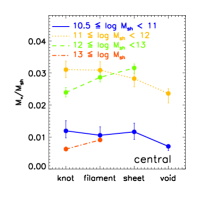
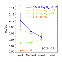
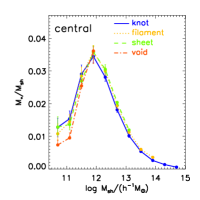
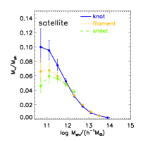
Figure 12: Galaxy stellar-to-subhalo mass ratio as a function of the cosmic web environment (top panels) and the subhalo mass (low panels) for central and satellite subhaloes.

4.2 galaxy stellar-to-subhalo mass ratio

The stellar masses of galaxies in SDSS are from the public catalog of Chang et al. (2015) . The subhalo masses are from the subhaloes by the SUBFIND algorithm (Springel et al., 2001) in ELUCID simulation. Linking galaxies in observation to subhaloes in simulation, we find that the galaxy stellar-to-subhalo mass ratio is a good proxy of the subhalo formation time, especially for galaxies in high-mass subhaloes. Therefore, it’s interesting to investigate the dependence of the galaxy stellar-to-subhalo mass ratio on the cosmic web environment.

The top panels of Figure 12 show the galaxy stellar-to-subhalo mass ratio as a function of the cosmic web environment for central and satellite galaxies, respectively. For central galaxies, in the mass ranges of $(10.5,11)$ and $(11,12)$, the stellar-to-subhalo mass ratios in knots are larger than those in filaments, sheets, or voids, while in the mass ranges of $(12,13)$ and $(13,\infty)$, the ratios in knots are smaller than those in filaments or sheets. For clarity, we also show the galaxy stellar-to-subhalo mass ratio as a function of the subhalo mass in different cosmic environment in the low panels of Figure 12. For central galaxies, the stellar-to-subhalo mass ratio has a peak at the subhalo mass $\sim 10^{12}\,h^{-1}{\rm M}_{\odot}$ and drops fast towards the low-mass or high-mass end. Similar to the dependence of the formation time on the cosmic web environment, there is a characteristic subhalo mass of $\sim 10^{12}\,h^{-1}{\rm M}_{\odot}$, below which the galaxy stellar-to-subhalo mass ratio is largest in konts, while above which it reverses.

For satellite galaxies, the dependence of the stellar-to-subhalo mass ratio on environment is similar to that of central galaxies. For satellite galaxies with their corresponding subhalo mass less than $\sim 10^{12}\,h^{-1}{\rm M}_{\odot}$, the stellar-to-subhalo mass ratio decreases from knots to filaments or sheets, while the ratio slightly increases from knots to filaments with mass larger than $\sim 10^{12}\,h^{-1}{\rm M}_{\odot}$. Note that no statistical results can be obtained in voids for satellite galaxies due to the limited number.

The general trends of the stellar-to-subhalo mass ratios on the cosmic web environment are quite consistent with those of the subhalo formation time, indicating that the former is indeed a good tracer of the latter.

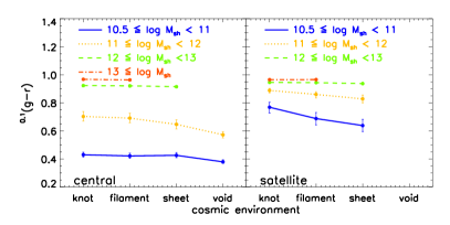
Figure 13: Galaxy colors as a function of the cosmic web environment for central (left panel) and satellite (right panel) galaxies with different corresponding subhalo mass $\log(M_{\rm sh}/(\,h^{-1}{\rm M}_{\odot}))$ in the ranges of $(10.5,11)$, $(11,12)$, $(12,13)$, and $(13,\infty)$.

4.3 galaxy color and specific star formation rate

Galaxy color is one of the most important variables in observation, and it’s tightly correlated with the galaxy specific star formation rate. In this section, we mainly focus on the dependence of galaxy color and specific star formation rate on the cosmic web environment.

Figure 13 shows the median values of galaxy colors as a function of the cosmic web environment for central and satellite galaxies, respectively. As expected, more massive galaxies have higher ${}^{0.1}(g-r)$ and tend to be redder. For centrals or satellites with subhalo mass less than $10^{12}\,h^{-1}{\rm M}_{\odot}$, galaxies in knots are redder than those in filaments, sheets, or voids. For galaxies in massive subhaloes with mass larger than $10^{12}\,h^{-1}{\rm M}_{\odot}$, there is no clear difference of galaxy colors in different cosmic web environments, since the color difference is negligible for galaxies in high-mass subhaloes, and galaxies in massive subhaloes are all equally red as shown in Figure 2.

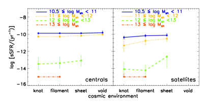
Figure 14: Specific star formation rate as a function of the cosmic web environment for central (left panel) and satellite (right panel) galaxies with different corresponding subhalo mass $\log(M_{\rm sh}/(\,h^{-1}{\rm M}_{\odot}))$ in the ranges of $(10.5,11)$, $(11,12)$, $(12,13)$, and $(13,\infty)$.

The specific star formation rates of galaxies are from the public catalog of Chang et al. (2015). The specific star formation rate has been extensively used as the indicator of galaxy quiescence to separate the quenched from the star-forming population (Favole et al., 2021).

Figure 14 shows the median values of galaxy specific star formation rates as a function of the cosmic web environment for central and satellite galaxies, respectively. For centrals or satellites, galaxies in knots have lower sSFRs than those in filaments, sheets, or voids, especially for galaxies with their corresponding subhalo mass less than $10^{13}\,h^{-1}{\rm M}_{\odot}$. This behavior is consistent with the environmental dependence of galaxy colors.

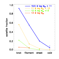
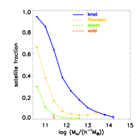
Figure 15: Satellite fraction as a function of the cosmic web environment (left panel) and the subhalo mass (right panel).

4.4 satellite fraction

The satellite fraction of galaxies as a function of luminosity or stellar mass is important for understanding the clustering of galaxies at fixed luminosity or stellar mass (Yang et al., 2012; Yang et al., 2018), the measurements of galaxy-galaxy lensing signals (Mandelbaum et al., 2006), and the quenching of central and satellite galaxies (Bluck et al., 2016). Using galaxy-subhalo pairs catalog, Yang et al. (2018) have shown that the satellite fraction decreasing with stellar mass, and red galaxies have significantly higher satellite fraction than bule galaxies, especially for low-mass galaxies. Using galaxy-galaxy weak lensing from SDSS, Mandelbaum et al. (2006) also found early-type galaxies have higher satellite fraction than late-type galaxies at a give stellar mass.

Since galaxies in older subhaloes are more likely to be satellite galaxies, at a given mass, satellite fraction is tightly correlated with the subhalo formation time. In this section, we investigate the dependence of satellite fraction on the cosmic web environment.

The left panel of Figure 15 shows the satellite fraction as a function of the cosmic web environment for galaxies in different mass subhaloes. The satellite fraction decreases from knots to filaments to sheets to voids, especially for low-mass galaxies. The right panel of Figure 15 shows the satellite fraction as a function of the subhalo mass. Generally, the satellite fraction significantly decreases with increasing subhalo mass in different cosmic web environment. At fixed mass, galaxies in knots have larger satellite fraction than those in filaments, sheets, or voids.

Since satellite fraction is strongly dependent on the cosmic web environment, more satellites in knots can result in the redder colors in knots for a sample of galaxies including centrals and satellites, considering that satellite galaxies are redder than central galaxies at fixed mass. As a consequence, the properties of central and satellite galaxies are separately investigated in the previous sections. The cosmic web environmental dependence of galaxy colors will be significantly amplified for total galaxies, if galaxies are not distinguished into central or satellite subsamples.

5 Summary

In this paper, combining galaxies from SDSS DR7 and subhaloes from the ELUCID simulation, we have investigated the relation between the formation time of subhaloes and the galaxy properties. Besides, we investigate the dependence of galaxy properties on the cosmic web environment, which is composed of knots, filaments, sheets, and voids, classified by the Hessian matrix of the density field (Zhang et al., 2009). The subhalo formation time is defined as the time at which the main branch progenitor reached half of its maximum mass. The galaxy stellar mass is estimated from Chang et al. (2015), and the subhalo mass is obtained from the matched subhalo in ELUCID simulation by the neighborhood abundance matching method (Yang et al., 2018). Due to the distinct assembly history of centrals and satellites, we investigated the properties of centrals and satellites separately. The following are our main findings:

• Central and satellite subhaloes have different formation time, and satellite subhaloes are older than central subhaloes at fixed mass. Central and satellite galaxies have different stellar-to-subhalo mass ratios at fixed subhalo mass, especially for galaxies in low-mass subhaloes. At fixed subhalo mass, satellite galaxies have significantly larger stellar mass than central galaxies, especially for galaxies in subhaloes with mass less than $10^{12}\,h^{-1}{\rm M}_{\odot}$.

• Galaxy stellar-to-subhalo mass ratio is tightly correlated with the subhalo formation time, and the formation redshifts increase with stellar-to-subhalo mass ratios, especially for galaxies in high-mass subhaloes.

• Subhalo formation time is dependent on the cosmic web environment. For central subhaloes, there is a characteristic subhalo mass of $\sim 10^{12}\,h^{-1}{\rm M}_{\odot}$, below which subhaloes in knots are older than subhaloes of the same mass in filaments, sheets or voids, while above which it reverses. For satellite subhaloes in low-mass range, subhaloes in knots are also oldest than those in other environments.

• The cosmic web environmental dependence of galaxy stellar-to-subhalo mass ratio is similar to that of the subhalo formation time. For centrals, there is a characteristic subhalo mass of $\sim 10^{12}\,h^{-1}{\rm M}_{\odot}$, below which the ratio decreases from knots to filaments to sheets to voids, above which it reverses.

• For centrals or satellites in subhaloes with mass less than $10^{12}\,h^{-1}{\rm M}_{\odot}$, galaxies in knots are redder than those in filaments, sheets, or voids. Above $10^{12}\,h^{-1}{\rm M}_{\odot}$, there is no clear difference of galaxy colors in different cosmic web environment.

• Satellite fraction is strongly dependent on the cosmic web environment, and decreases from knots to filaments to sheets to voids, especially for low-mass galaxies.

To conclude, we remark that galaxy stellar-to-subhalo mass ratio is a good proxy of the subhalo formation time, especially for galaxies in high-mass subhaloes. The environmental dependence of formation time is similar to that of galaxy stellar-to-subhalo mass ratio. Low-mass subhaloes show a decreasing formation redshifts and galaxy stellar-to-subhalo mass ratios from knots to voids, while the trend reverses in high-mass subhaloes.

Data availability

The data underlying this article will be shared on reasonable request to the corresponding author.

References

- Abazajian et al. (2009) Abazajian K. N., et al., 2009, ApJS, 182, 543
- Alonso et al. (2015) Alonso D., Eardley E., Peacock J. A., 2015, MNRAS, 447, 2683
- Alonso et al. (2016) Alonso D., Hadzhiyska B., Strauss M. A., 2016, MNRAS, 460, 256
- Alpaslan et al. (2015) Alpaslan M., et al., 2015, MNRAS, 451, 3249
- Alpaslan et al. (2016) Alpaslan M., et al., 2016, MNRAS, 457, 2287
- Aragón-Calvo et al. (2007) Aragón-Calvo M. A., Jones B. J. T., van de Weygaert R., van der Hulst J. M., 2007, A&A, 474, 315
- Baldry et al. (2004) Baldry I. K., Glazebrook K., Brinkmann J., Ivezić Ž., Lupton R. H., Nichol R. C., Szalay A. S., 2004, ApJ, 600, 681
- Bell et al. (2003) Bell E. F., McIntosh D. H., Katz N., Weinberg M. D., 2003, ApJS, 149, 289
- Blanton & Berlind (2007) Blanton M. R., Berlind A. A., 2007, ApJ, 664, 791
- Blanton & Roweis (2007) Blanton M. R., Roweis S., 2007, AJ, 133, 734
- Blanton et al. (2003) Blanton M. R., et al., 2003, AJ, 125, 2348
- Blanton et al. (2005) Blanton M. R., et al., 2005, AJ, 129, 2562
- Bluck et al. (2016) Bluck A. F. L., et al., 2016, MNRAS, 462, 2559
- Bond et al. (1996) Bond J. R., Kofman L., Pogosyan D., 1996, Nature, 380, 603
- Brouwer et al. (2016) Brouwer M. M., et al., 2016, MNRAS, 462, 4451
- Campbell et al. (2018) Campbell D., van den Bosch F. C., Padmanabhan N., Mao Y.-Y., Zentner A. R., Lange J. U., Jiang F., Villarreal A., 2018, MNRAS, 477, 359
- Chang et al. (2015) Chang Y.-Y., van der Wel A., da Cunha E., Rix H.-W., 2015, ApJS, 219, 8
- Chaves-Montero et al. (2016) Chaves-Montero J., Angulo R. E., Schaye J., Schaller M., Crain R. A., Furlong M., Theuns T., 2016, MNRAS, 460, 3100
- Chen et al. (2017) Chen Y.-C., et al., 2017, MNRAS, 466, 1880
- Chen et al. (2020) Chen Y., Mo H. J., Li C., Wang H., Yang X., Zhang Y., Wang K., 2020, ApJ, 899, 81
- Conroy et al. (2006) Conroy C., Wechsler R. H., Kravtsov A. V., 2006, ApJ, 647, 201
- Contreras et al. (2019) Contreras S., Zehavi I., Padilla N., Baugh C. M., Jiménez E., Lacerna I., 2019, MNRAS, 484, 1133
- Contreras et al. (2020) Contreras S., Angulo R., Zennaro M., 2020, arXiv e-prints, p. arXiv:2012.06596
- Cooper et al. (2010) Cooper M. C., Gallazzi A., Newman J. A., Yan R., 2010, MNRAS, 402, 1942
- Correa & Schaye (2020) Correa C. A., Schaye J., 2020, MNRAS, 499, 3578
- Davis et al. (1985) Davis M., Efstathiou G., Frenk C. S., White S. D. M., 1985, ApJ, 292, 371
- Dragomir et al. (2018) Dragomir R., Rodríguez-Puebla A., Primack J. R., Lee C. T., 2018, MNRAS, 476, 741
- Dvornik et al. (2017) Dvornik A., et al., 2017, MNRAS, 468, 3251
- Eardley et al. (2015) Eardley E., et al., 2015, MNRAS, 448, 3665
- Favole et al. (2021) Favole G., Montero-Dorta A. D., Artale M. C., Contreras S., Zehavi I., Xu X., 2021, arXiv e-prints, p. arXiv:2101.10733
- Ferreras et al. (2019) Ferreras I., Hopkins A. M., Lagos C., Sansom A. E., Scott N., Croom S., Brough S., 2019, MNRAS, 487, 435
- Gao & White (2007) Gao L., White S. D. M., 2007, MNRAS, 377, L5
- Gao et al. (2005) Gao L., Springel V., White S. D. M., 2005, MNRAS, 363, L66
- Goh et al. (2019) Goh T., et al., 2019, MNRAS, 483, 2101
- Hahn et al. (2007a) Hahn O., Porciani C., Carollo C. M., Dekel A., 2007a, MNRAS, 375, 489
- Hahn et al. (2007b) Hahn O., Carollo C. M., Porciani C., Dekel A., 2007b, MNRAS, 381, 41
- Hearin & Watson (2013) Hearin A. P., Watson D. F., 2013, MNRAS, 435, 1313
- Hearin et al. (2014) Hearin A. P., Watson D. F., Becker M. R., Reyes R., Berlind A. A., Zentner A. R., 2014, MNRAS, 444, 729
- Jing et al. (2007) Jing Y. P., Suto Y., Mo H. J., 2007, ApJ, 657, 664
- Kraljic et al. (2018) Kraljic K., et al., 2018, MNRAS, 474, 547
- Lacerna & Padilla (2012) Lacerna I., Padilla N., 2012, MNRAS, 426, L26
- Lacerna et al. (2014) Lacerna I., Padilla N., Stasyszyn F., 2014, MNRAS, 443, 3107
- Laigle et al. (2018) Laigle C., et al., 2018, MNRAS, 474, 5437
- Lange et al. (2019) Lange J. U., van den Bosch F. C., Zentner A. R., Wang K., Villarreal A. S., 2019, MNRAS, 487, 3112
- Lim et al. (2016) Lim S. H., Mo H. J., Wang H., Yang X., 2016, MNRAS, 455, 499
- Lin et al. (2016) Lin Y.-T., Mandelbaum R., Huang Y.-H., Huang H.-J., Dalal N., Diemer B., Jian H.-Y., Kravtsov A., 2016, ApJ, 819, 119
- Luber et al. (2019) Luber N., van Gorkom J. H., Hess K. M., Pisano D. J., Fernández X., Momjian E., 2019, AJ, 157, 254
- Mahajan et al. (2018) Mahajan S., Singh A., Shobhana D., 2018, MNRAS, 478, 4336
- Malavasi et al. (2017) Malavasi N., et al., 2017, MNRAS, 465, 3817
- Mandelbaum et al. (2006) Mandelbaum R., Seljak U., Kauffmann G., Hirata C. M., Brinkmann J., 2006, MNRAS, 368, 715
- Mandelbaum et al. (2016) Mandelbaum R., Wang W., Zu Y., White S., Henriques B., More S., 2016, MNRAS, 457, 3200
- Mansfield & Kravtsov (2020) Mansfield P., Kravtsov A. V., 2020, MNRAS, 493, 4763
- Matthee et al. (2017) Matthee J., Schaye J., Crain R. A., Schaller M., Bower R., Theuns T., 2017, MNRAS, 465, 2381
- Miyatake et al. (2016) Miyatake H., More S., Takada M., Spergel D. N., Mandelbaum R., Rykoff E. S., Rozo E., 2016, Phys. Rev. Lett., 116, 041301
- Moster et al. (2010) Moster B. P., Somerville R. S., Maulbetsch C., van den Bosch F. C., Macciò A. V., Naab T., Oser L., 2010, ApJ, 710, 903
- Musso et al. (2018) Musso M., Cadiou C., Pichon C., Codis S., Kraljic K., Dubois Y., 2018, MNRAS, 476, 4877
- Obuljen et al. (2020) Obuljen A., Percival W. J., Dalal N., 2020, J. Cosmology Astropart. Phys., 2020, 058
- Paranjape et al. (2018a) Paranjape A., Hahn O., Sheth R. K., 2018a, MNRAS, 476, 3631
- Paranjape et al. (2018b) Paranjape A., Hahn O., Sheth R. K., 2018b, MNRAS, 476, 5442
- Ramakrishnan & Paranjape (2020) Ramakrishnan S., Paranjape A., 2020, MNRAS, 499, 4418
- Ramakrishnan et al. (2019) Ramakrishnan S., Paranjape A., Hahn O., Sheth R. K., 2019, MNRAS, 489, 2977
- Reddick et al. (2013) Reddick R. M., Wechsler R. H., Tinker J. L., Behroozi P. S., 2013, ApJ, 771, 30
- Rodriguez et al. (2020) Rodriguez F., Montero-Dorta A. D., Angulo R. E., Artale M. C., Merchán M., 2020, arXiv e-prints, p. arXiv:2011.00014
- Salcedo et al. (2020) Salcedo A. N., et al., 2020, arXiv e-prints, p. arXiv:2010.04176
- Sheth & Tormen (2004) Sheth R. K., Tormen G., 2004, MNRAS, 350, 1385
- Singh et al. (2020) Singh A., Mahajan S., Bagla J. S., 2020, MNRAS, 497, 2265
- Sinigaglia et al. (2020) Sinigaglia F., Kitaura F.-S., Balaguera-Antolínez A., Nagamine K., Ata M., Shimizu I., Sánchez-Benavente M., 2020, arXiv e-prints, p. arXiv:2012.06795
- Springel (2005) Springel V., 2005, MNRAS, 364, 1105
- Springel et al. (2001) Springel V., White S. D. M., Tormen G., Kauffmann G., 2001, MNRAS, 328, 726
- Springel et al. (2005) Springel V., et al., 2005, Nature, 435, 629
- Springel et al. (2020) Springel V., Pakmor R., Zier O., Reinecke M., 2020, arXiv e-prints, p. arXiv:2010.03567
- Tinker et al. (2008) Tinker J. L., Conroy C., Norberg P., Patiri S. G., Weinberg D. H., Warren M. S., 2008, ApJ, 686, 53
- Tinker et al. (2017) Tinker J. L., Wetzel A. R., Conroy C., Mao Y.-Y., 2017, MNRAS, 472, 2504
- Tinker et al. (2018) Tinker J. L., Hahn C., Mao Y.-Y., Wetzel A. R., Conroy C., 2018, MNRAS, 477, 935
- Tojeiro et al. (2017) Tojeiro R., et al., 2017, MNRAS, 470, 3720
- Tweed et al. (2017) Tweed D., Yang X., Wang H., Cui W., Zhang Y., Li S., Jing Y. P., Mo H. J., 2017, ApJ, 841, 55
- Villarreal et al. (2017) Villarreal A. S., et al., 2017, MNRAS, 472, 1088
- Wang et al. (2007) Wang H. Y., Mo H. J., Jing Y. P., 2007, MNRAS, 375, 633
- Wang et al. (2011) Wang H., Mo H. J., Jing Y. P., Yang X., Wang Y., 2011, MNRAS, 413, 1973
- Wang et al. (2012) Wang H., Mo H. J., Yang X., van den Bosch F. C., 2012, MNRAS, 420, 1809
- Wang et al. (2013) Wang L., Weinmann S. M., De Lucia G., Yang X., 2013, MNRAS, 433, 515
- Wang et al. (2014) Wang H., Mo H. J., Yang X., Jing Y. P., Lin W. P., 2014, ApJ, 794, 94
- Wang et al. (2016) Wang H., et al., 2016, ApJ, 831, 164
- Watson et al. (2015) Watson D. F., et al., 2015, MNRAS, 446, 651
- Wechsler et al. (2006) Wechsler R. H., Zentner A. R., Bullock J. S., Kravtsov A. V., Allgood B., 2006, ApJ, 652, 71
- White & Rees (1978) White S. D. M., Rees M. J., 1978, MNRAS, 183, 341
- Xu et al. (2020a) Xu X., Zehavi I., Contreras S., 2020a, arXiv e-prints, p. arXiv:2007.05545
- Xu et al. (2020b) Xu W., et al., 2020b, MNRAS, 498, 1839
- Yang et al. (2006) Yang X., Mo H. J., van den Bosch F. C., 2006, ApJ, 638, L55
- Yang et al. (2007) Yang X., Mo H. J., van den Bosch F. C., Pasquali A., Li C., Barden M., 2007, ApJ, 671, 153
- Yang et al. (2012) Yang X., Mo H. J., van den Bosch F. C., Zhang Y., Han J., 2012, ApJ, 752, 41
- Yang et al. (2017) Yang X., et al., 2017, ApJ, 848, 60
- Yang et al. (2018) Yang X., et al., 2018, ApJ, 860, 30
- York et al. (2000) York D. G., et al., 2000, AJ, 120, 1579
- Yuan et al. (2020) Yuan S., Hadzhiyska B., Bose S., Eisenstein D. J., Guo H., 2020, arXiv e-prints, p. arXiv:2010.04182
- Zentner et al. (2014) Zentner A. R., Hearin A. P., van den Bosch F. C., 2014, MNRAS, 443, 3044
- Zhang et al. (2009) Zhang Y., Yang X., Faltenbacher A., Springel V., Lin W., Wang H., 2009, ApJ, 706, 747
- Zhang et al. (2021) Zhang Y., Yang X., Guo H., 2021, MNRAS, 500, 1895
- Zu & Mandelbaum (2016) Zu Y., Mandelbaum R., 2016, MNRAS, 457, 4360
- Zu et al. (2017) Zu Y., Mandelbaum R., Simet M., Rozo E., Rykoff E. S., 2017, MNRAS, 470, 551
- van den Bosch & Ogiya (2018) van den Bosch F. C., Ogiya G., 2018, MNRAS, 475, 4066